Statistical properties of the aftershocks of stock market crashes revisited: Analysis based on the 1987 crash, financial-crisis-2008 and COVID-19 pandemic

Abstract

During any unique crisis, panic sell-off leads to a massive stock market crash that may continue for more than a day, termed as mainshock. The effect of a mainshock in the form of aftershocks can be felt throughout the recovery phase of stock price. As the market remains in stress during recovery, any small perturbation leads to a relatively smaller aftershock. The duration of the recovery phase has been estimated using structural break analysis. We have carried out statistical analyses of 1987 stock market crash, 2008 financial crisis and 2020 COVID-19 pandemic considering the actual crash-times of the mainshock and aftershocks. Earlier, such analyses were done considering absolute one-day return, which cannot capture a crash properly. The results show that the mainshock and aftershock in the stock market follows the Gutenberg-Richter (GR) power law. Further, we obtained higher $\beta$ value for the COVID-19 crash compared to the financial-crisis-2008 from the GR law. This implies that the recovery of stock price during COVID-19 may be faster than the financial-crisis-2008. The result is consistent with the present recovery of the market from the COVID-19 pandemic. The analysis shows that the high magnitude aftershocks are rare, and low magnitude aftershocks are frequent during the recovery phase. The analysis also shows that the distribution $P(\tau_{i})$ follows the generalized pareto distribution, i.e., $\displaystyle~{}P(\tau_{i})\propto\frac{1}{\{1+\lambda(q-1)\tau_{i}\}^{\frac{1}{(q-1)}}}$, where $\lambda$ and $q$ are constants and $\tau_{i}$ is the inter-occurrence time. This analysis may help investors to restructure their portfolio during a market crash.

I Introduction

Complex dynamical systems, such as stock market, earth crust, climate, ocean show rare phenomena in the form of price crash, earthquake, storm and tsunami under certain crisis Sornette (2017); McNamara et al. (2015); Sarlis et al. (2018); Pisarenko and Sornette (2003); Nguyen, Bhatti, and Henry (2017); Piccoli et al. (2017); Zhang et al. (2009); Sornette and Johansen (1998); Sornette, Johansen, and Bouchaud (1996); Mahata et al. (2021a). Some of these rare events which can be termed as a main-shock, leads to a series of smaller aftershocks Sornette (2017); Sornette, Johansen, and Bouchaud (1996); Abe and Suzuki (2004); Siokis (2012). The dynamics of such systems can be characterized statistically by power-law distributions Bak et al. (2002); Bai and Zhu (2010); Gabaix et al. (2007); Siokis (2012); Selçuk (2004); Kapopoulos and Siokis (2005). In the stock market, a rare event occurs in the form of a major crash due to the emergence of a new and novel risk factor, for which investors are not prepared Albuquerque et al. (2020); Mazur, Dang, and Vega (2020). The new unique risk leads to a wide fluctuation in price and volume because of the investors’ irrational behavior, and causes a massive crash Mazur, Dang, and Vega (2020); Lyócsa et al. (2020); Baker et al. (2020); Wang et al. (2009); Barlevy and Veronesi (2003).

The reasons for the crash in stock market is the formation of instability due to herding behavior, speculation, overvaluation and emergence of novel risk factors Chiang and Zheng (2010); Tan et al. (2008); White (1990); Choudhry (1996); Carlson (2007); Grant (1990); Mahata et al. (2021a); Mazur, Dang, and Vega (2020); Lyócsa et al. (2020); Baker et al. (2020); Wang et al. (2009); Barlevy and Veronesi (2003). The financial crisis and pandemic have a devastating effect on all the economic sectors that lasts for several months to years. As a result stock market remains in stress till the economy starts to recover Sornette and Johansen (1997); Mazur, Dang, and Vega (2020); Mahata et al. (2021b). During the stressed period after the major crash, a number of aftershocks of comparatively smaller magnitudes occur due to investors’ cautious approach in investment Siokis (2012); Selçuk (2004); Kapopoulos and Siokis (2005); Netter and Mitchell (1989); Hong and Stein (2003). Understanding the properties of the mainshock and aftershocks are essential for the investment decision during a crisis.

Statistical properties of the volatility of stock price, volume, daily returns of stock market have been extensively studied using the statistical tools like correlation, power law, multifractality and many other techniques Gopikrishnan et al. (2000); Oh et al. (2011); Liu et al. (1999); Mantegna and Stanley (1997); Cont (2001); Restocchi, McGroarty, and Gerding (2019); Da Cunha and da Silva (2020); Noh (2000); Hamao, Masulis, and Ng (1990); Wang, Shang, and Ge (2012); Turiel and Pérez-Vicente (2003). However, limited studies on the statistical properties of crash in stock price are carried out.  Siokis (2012); Selçuk (2004); Kapopoulos and Siokis (2005); Potirakis, Zitis, and Eftaxias (2013); Petersen et al. (2010). Further, these studies have some limitations with regard to the length of crashes and duration of its effect  Siokis (2012); Selçuk (2004); Kapopoulos and Siokis (2005). Hence, a detailed statistical analysis is required to understand the stock market crash.

The analysis methods that are applied to study the geophysical phenomena have also been applied to understand the statistical properties of the price crash and subsequent aftershocks  Siokis (2012); Selçuk (2004); Kapopoulos and Siokis (2005). The Gutenberg-Richter (GR) power law and Omori law are frequently used to explain such statistical properties  Siokis (2012); Selçuk (2004); Kapopoulos and Siokis (2005); Potirakis, Zitis, and Eftaxias (2013); Petersen et al. (2010). In these studies, the mainshock and aftershocks were identified for intra-day data with the one-minute absolute log return Petersen et al. (2010), and 60, 100 and 240 days data with the one-day absolute log return Selçuk (2004); Lillo and Mantegna (2003); Siokis (2012); Kapopoulos and Siokis (2005); Selçuk (2004). Omori law is also seen to hold not only for stock returns but also for stock volatilities Mu and Zhou (2008). Models have also been developed to predict the crash in the stock market considering similarities between the stock return after a major crash with aftershock activities during an earthquake Gresnigt, Kole, and Franses (2015). However, all these analyses have the following limitations:

1. As the market crash during a severe crisis can continue for more than a day Sornette and Johansen (1997); Sornette, Johansen, and Bouchaud (1996); Sornette and Johansen (1998), the mainshock and aftershock cannot be limited to a single day or minute return.

2. After the implementation of the circuit breakers in the market, it takes more than a day to complete an intense crash. Hence, taking one day fall as a mainshock or aftershock may be erroneous.

3. When one-day absolute log return is considered, both the crash and recovery act as a crash.

4. The duration of the aftershock sequence has been taken arbitrarily though the effect of major crash may stay for a longer/shorter period in the market and economy. Hence, identifying the proper duration of the mainshock is very essential to analyze the statistics of shocks.

This paper aims to study the statistical properties of stock market crash by addressing the above limitations. We have estimated the actual crash-time of mainshock and aftershocks as the cumulative consecutive fall of a stock price. During the estimation of continuous fall, we have ignored the smaller intermediate weak recoveries. Maximum magnitude of these weak recoveries is 7.0% of the mainshock. If the secondary crashes are larger than 7.0% of the main crash, they are considered as an aftershock. Further, the structural break analysis method Bai and Perron (1998, 2003) is applied to estimate the duration of influence of the mainshock. The aftershocks that happened during this duration are considered for the analysis. We obtained that the aftershock sequence follows the GR power law. Adjusted $R^{2}$ and P-value from K-S test are calculated to verify that the data fits well with the GR power law. $R^{2}$ and P-value indicates how well the data fits with the power law. The P-value greater than 0.1 and 0.05 are considered as a good fit between the power law distribution and the data Clauset, Shalizi, and Newman (2009); Taleghani, Salehi, and Shakibaiee (2019). We have calculated the values of $R^{2}$ and P-value to show that the power law distribution is a good fit to the data. We also intend to extract some new information about the possible occurrence of aftershocks during the latest stock market crash in 2020 due to the COVID-19 pandemic.

The paper is organised as follows: Sec. II discusses about the methods used for the analysis. Sec. III provides the data description. Sec. IV discusses about the results obtained from the analysis. Finally, Sec. V includes the summary of the paper and our concluding remarks.

II Methodology

II.1 Gutenberg-Richter power law

The Gutenberg-Richter (GR) power law is one of the important empirical law that is applied to study the statistical properties of an earthquake in geophysics Sornette and Sornette (1999); Gutenberg and Richter (1944). It shows the relationship between the number of earthquakes (aftershocks) to the magnitude of each earthquake. It states that the cumulative number of earthquakes ($N$) with magnitude $M$ larger than or equal to $M$ is proportional to $M$ and is given by

$$\log_{10}N(M)=\alpha-\beta M$$ (1)

Where $\alpha$ and $\beta$ are two positive constants. The slope $\beta$ shows the relationship between the convergence process after a shock to its magnitude.

Eqn. 1 is also used to explain the aftershock sequence in the stock market after a major market crash. The large absolute value of $\beta$ indicates that the stock/index will experience a heavy-sized aftershocks but will get to a normal period very shortly and low absolute value of $\beta$ implies that the stock/index will in general have a longer recovery period. The constant parameter $\alpha$ represents the number of remaining aftershocks, which does not depend on the magnitude of the aftershocks Siokis (2012); Kapopoulos and Siokis (2005). In our case, magnitude (M) of the mainshock and aftershock is defined as the difference in the stock price from the day of fall till there is strong sign of recovery i.e., recovery of 7.0% or more of the main crash.

II.2 Degree of Nonstationarity

In order to test nonstationarity, Degree of nonstationarity (DNS) test is applied. DNS is defined as Chowdhury et al. (2017); Huang et al. (1998); Mahata et al. (2021a)

$$DNS(\omega)=\frac{1}{T}\int_{0}^{T}[1-\frac{H(t,\omega)}{h(\omega)}]dt$$ (2)

Here [0, $T$] is the time window, $h(\omega)$ is the marginal spectrum which is written as $h(\omega)=\frac{1}{T}\int_{0}^{T}H(t,\omega)dt$ and $H(t,\omega)$ is the Hilbert spectrum. Hilbert spectrum is defined as $H(t,\omega)=Re\sum_{j}M_{j}(t)~{}e^{i\int{\omega_{j}(t)dt}}$, where $M_{j}(t)$ is the amplitude and $\omega_{j}(t)$ is the frequency.

Eqn. 2 shows the stationarity of a time series data as a function of frequency. In case of a stationary data, Hilbert spectrum is independent of time and will consist of horizontal line. Hence, $DNS(\omega)$ will be zero. However, when the $H(t,\omega)$ is time dependent $DNS(\omega)$ will not be zero Chowdhury et al. (2017); Huang et al. (1998); Mahata et al. (2021a).

II.3 Structural Break Analysis Technique

The structural break analysis method developed by Bai and Perron (1998, 2003) Bai and Perron (1998, 2003) is applied to capture the structural changes in a stock price time series. As the structural breaks emerge for a sudden change in a time series, it helps us to identify the duration of the influence of a crisis Bai and Perron (1998, 2003); Mahata, Bal, and Nurujjaman (2020). A detailed procedure of the estimation of structural break is given below Bai and Perron (1998, 2003).

Let us consider the following structural change model with $m$ break points

$$y_{t}=x_{t}^{{}^{\prime}}\zeta+z_{t}^{{}^{\prime}}\delta_{j}+u_{t},~{}~{}~{}t=T_{j-1}+1,.....,T_{j}$$ (3)

where, $j=1,...,~{}m$. $x_{t}(p\times 1)$ and $z_{t}(q\times 1)$ are vectors of covariates and $u_{t}$ is the disturbance at time t. The break dates ($T_{1},...,T_{m}$) are explicitly treated as unknown. The purpose is to estimate the unknown regression coefficients $\zeta$, $\delta_{j}$ and the break dates. For each $m$-partition ($T_{1},...,T_{m}$), denoted by $T_{j}$, the associate least square estimates of $\zeta$, $\delta_{j}$ are obtained by minimizing the following objective function

$$\sum_{i=1}^{m+1}\sum_{t=T_{i-1}+1}^{T_{i}}(y_{t}-x_{t}^{{}^{\prime}}\zeta-z_{t}^{{}^{\prime}}\delta_{i})^{2}$$ (4)

Let $\hat{\zeta}(T_{j})$ and $\hat{\delta}(T_{j})$ denote the resulting estimates that minimize the objective function. The sum of squared residual, $SSR_{T}(T_{1},....,T_{m})$ is obtained by substituting $\hat{\zeta}(T_{j})$ and $\hat{\delta}(T_{j})$ in the above objective function. The resulting estimated break dates $T_{1},....,T_{m}$ are obtained as

$$\{(\hat{T_{1}}),...,(\hat{T_{m}})\}=arg\min_{T_{1},...T_{m}}SSR_{T}\{T_{1},....,T_{m}\}$$ (5)

where the minimization is done over all partitions $(T_{1},...,T_{m})$. The break date estimators are global minimizer of the objective function. Let $v(i,j)$ be the recursive residual at time $j$ obtained using a sample that starts at date $i$. $SSR(i,j)$ is the sum of squared residual obtained by applying least-squares to a segment that starts at date $i$ and ends at date $j$ with $SSR(i,j)=SSR(i,j-1)+v(i,j)^{2}$. In order to evaluate the global optimal partition, a dynamical programming approach is applied on the sums of squared residual of all the relevant combination of ($i,j$) segments. Finally, $m$ break points have been obtained from the global optimal partition function $SSR(T_{m,K})$ by using first $K$ observation as given in the following recursive equation.

$$SSR(T_{m,K})=\min_{mh\leq K\leq K-h}\{SSR(T_{m-1,j})+SSR(j+1,K)\}$$ (6)

In our regression procedure, we have taken upto 3-break points or four segments and $z_{t}=\{1\}$ as a constant regressor.

III Data Analysed

In this paper, analysis of the stock price crashes are carried out using the daily closing price of indices and companies. The stock data were taken from Yahoo Finance Yah . We have analyzed the shocks due to the 1987 crash, the financial-crisis-2008 and the 2020 COVID-19 pandemic. In case of the 1987 crash, we have taken DJIA index data as daily closing price of other companies were unavailable.

We have taken fourteen dominant world stock indices: Nasdaq (USA), DJIA (USA), HSI (Hongkong), BEL20 (Belgium), IBOVESPA (Brazil), BSE SENSEX (India), DAX (Germany), IBEX35 (Spain), IPC (Mexico), Nifty50 (India), NIKKEI225 (Japan), S&P500 (USA), SSE (China), CAC40 (France) and five Indian sectoral indices. The reason for choosing these indices are that they broadly represent the activity of world stock markets. Further, we have also taken thirty-two important companies that are listed in different leading worldwide stock exchanges.

IV Results and Discussion

In this section, we have presented the results of analysis of the mainshock and its subsequent aftershocks of the 1987 crash, the financial-crisis-2008 and the 2020 COVID-19 pandemic using our proposed definition of market crash. We have calculated the influence time length of these crashes using 3-point structural break analysis. All the stocks mentioned in Sec. III have been analyzed and their results are discussed herewith.

Figure 1: It represents the DNS plot of S&P 500 index and Amazon Inc. during (a) the financial-crisis-2008 and (b) the 2020 COVID-19 pandemic. The plots clearly show that the stock prices are non-stationary.

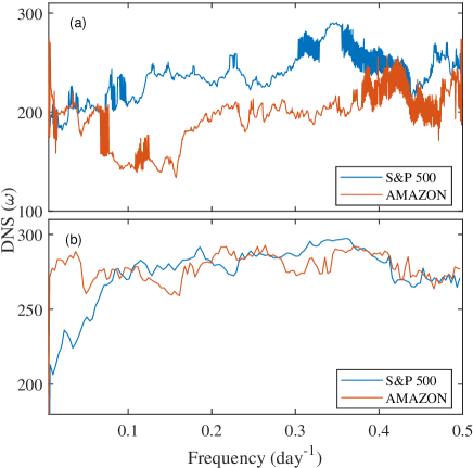
We have carried out the degree of non-stationarity (DNS) test for all the stocks and indices. Fig. 1 (a) and (b) represent the DNS($\omega$) plot of S&P 500 index and Amazon Inc. during the financial-crisis-2008 and the 2020 COVID-19 pandemic, respectively. DNS($\omega$) shows whether the time series data is stationary or not. DNS vs. $\omega$ plot is a horizontal straight line for a stationary time series. The DNS($\omega$) is not a horizontal straight line for nonstationary time series. Fig. 1 (a) and (b) show that the time series data are nonstationary as DNS vs $\omega$ plot are not a straight line. The DNS test show that the remaining indices and companies are also nonstationary. As the time series data are nonstationary, the structural break analysis is carried out to estimate the crash and recovery points.

IV.1 The crash of 1987

Figure 2: It represents the daily closing price of DJIA index from January 1987 to December 1989. The vertical dotted lines represent the structural break points.

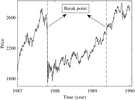
We first investigate the DJIA index from 1987 to 1990 during and after the Black Monday crash occurred at New York Stock Exchange (NYSE) that was considered one of the worst crash in the history of the NYSE. We found that the crash continued for eleven consecutive days. Hence, this consecutive eleven days fall is the actual crash-time and should be considered as a single crash. Fig. 2 represents the daily closing price of DJIA index during that period. In order to identify the number of aftershocks due to the mainshock of the 1987 crash, the duration of the influence is identified using the structural break analysis as given in Subsec. II.3. The closest breakpoints are shown by the vertical dotted lines in Fig. 2. The first vertical dotted line represents the starting point of the mainshock, and the second dotted line represents the end of the effect of the mainshock. Hence, the time of influence of the 1987 crash is from the time of the main crash till the end of 1989. The identified period is consistent with the recovery of the market.

Figure 3: The figure represents the plot between cumulative number of events ($N$) and the corresponding magnitude ($M$) of the 1987 crash.

Figure 4: Solid line represents the daily closing price of S&P500 index from April 2006 to December 2012. The dashed line represents the quarterly GDP growth rate of USA from 2006 to 2012. The vertical lines represent the structural break points.

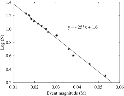
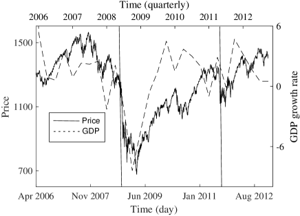
Fig. 3 shows the log-log plot between cumulative number of events (N) and its corresponding magnitude (M) of DJIA index during the 1987 crash. We performed a fit with the functional form of Eq. 1. The typical plot of $\log(N)$ vs. $\log(M)$ describes the empirical data well for the study period, i.e., the 1987 crash and its aftershocks follow the GR power law. The straight line represents the best fit, and the values of $\alpha$ and $\beta$ mentioned in Eqn. 1 are 1.6 and 25.0, respectively. The values of $R^{2}$ and P-value are 0.988 and 0.998, respectively. The figure clearly shows that the aftershocks with high magnitude are comparatively less than aftershocks with low magnitude. This should be the case as index generally does not fall with a high magnitude regularly. We have also obtained similar paradigmatic behavior of the leading stock price indices and companies due to the financial-crisis-2008 and the 2020 COVID-19 pandemic, and the detailed analysis are given below.

IV.2 The financial-crisis-2008

In Fig. 4, the solid line and dashed line represent the daily closing price of S&P 500 index from 2006 to 2012 and the quarterly GDP growth rate of USA from 2006 to 2012, respectively. The vertical solid lines are the structural breaks obtained for the financial-crisis-2008. The financial crisis can be clearly captured from these solid vertical lines. The closest breakpoints of the mainshock and recovery are mid of 2008 and end of 2011, respectively. Hence, we have taken the data from the time of mainshock till the end of 2011 to analyze the influence of the mainshock. Similar analyses have been carried out for the rest of the 50 companies and indices. Detailed analysis of all the indices and companies are given in Table 1.

Index/Company	The financial-crisis-2008						The COVID-19 Crisis
	% fall	N.A.S	$\alpha$	$\beta$	P-value	$R^{2}$	%fall	N.A.S	$\alpha$	$\beta$	P-value	$R^{2}$
NCI	22	26	1.7	14.0	0.892	0.987	14	19	1.6	39.0	0.741	0.917
HSI	29	29	1.7	13.0	0.741	0.923	15	13	1.4	28.0	0.995	0.933
BEL20 Index	24	27	1.7	13.0	0.995	0.985	30	17	1.5	30.0	0.930	0.946
IBOVESPA Index	29	26	1.6	9.9	0.892	0.967	21	16	1.4	17.0	0.912	0.969
BSE Index	25	22	1.7	13.0	0.979	0.964	20	13	1.2	12.0	0.828	0.900
DAX Index	27	27	1.6	11.0	0.698	0.967	28	16	1.5	34.0	0.912	0.946
DJIA Index	22	21	1.6	14.0	0.797	0.935	15	18	1.3	17.0	0.709	0.938
IBEX35 Index	25	22	1.7	13.0	0.979	0.964	20	13	1.2	12.0	0.828	0.894
IPC Index	26	24	1.3	8.2	0.953	0.977	13	12	1.3	26.0	0.991	0.970
Nifty50 Index	22	18	1.7	14.0	0.998	0.962	17	11	1.3	24.0	0.985	0.940
NIKKEI225 Index	32	26	1.7	12.0	0.992	0.987	29	13	1.2	26.0	0.433	0.967
S&P500 Index	23	27	1.7	13.0	0.698	0.966	14	13	1.3	17.0	0.995	0.944
SSE Index	26	18	1.5	9.7	0.945	0.987	12	11	1.2	19.0	0.991	0.909
CAC40 Index	27	34	1.8	13.0	0.962	0.984	29	14	1.5	28.0	0.862	0.918
Nifty Realty	41	51	1.9	9.2	0.850	0.975	19	15	1.3	12.0	0.998	0.917
Nifty Pharma	26	11	1.3	9.7	0.985	0.931	15	11	1.3	22.0	0.985	0.919
Nifty IT	22	28	1.8	15.0	0.490	0.989	5	12	1.3	35.0	0.433	0.966
Nifty Bank	32	44	1.8	9.8	0.777	0.975	33	17	1.5	19.0	0.998	0.917
Nifty FMCG	21	19	1.5	15.0	0.462	0.973	23	8	1.1	15.0	0.929	0.903
Adidas AG	29	32	1.8	14.0	0.951	0.971	32	18	1.4	19.0	0.945	0.950
Amazon Inc.	29	39	1.9	15.0	0.981	0.985	13	23	1.5	22.0	0.842	0.980
3M Co.	26	31	1.7	14.0	0.56	0.945	14	15	1.4	23.0	0.998	0.925
BASF SE	31	36	1.8	12.0	0.971	0.969	28	19	1.5	19.0	0.956	0.989
TCS Ltd.	23	39	2.0	18.0	0.884	0.969	17	19	1.5	26.0	0.956	0.962
Daikin Industries	43	48	1.9	10.0	0.480	0950	24	11	1.4	26.0	0.985	0.888
Bajaj Fin. Ltd.	48	40	1.9	13.0	0.983	0.980	23	22	1.5	13.0	0.990	0.970
Braskem	43	38	1.7	8.7	0.693	0.959	49	21	1.5	13.0	0.531	0.960
BPCL	26	38	1.8	11.0	0.978	0.990	20	16	1.3	12.0	0.912	0.969
Canon Inc.	26	31	1.9	17.0	0.998	0.985	25	18	1.5	22.0	0.673	0.940
CCCL	33	45	1.9	11.0	0.929	0.992	24	17	1.5	19.0	0.673	0.970
HDFC Bank Ltd.	26	27	1.8	16.0	0.905	0.977	29	17	1.4	17.0	0.930	0.979
Infosys Ltd.	25	29	1.8	14.0	0.72	0.98	30	18	1.3	22.0	0.995	0.993
Intel Corp.	27	39	2.0	17.0	0.884	0.975	10	20	1.5	24.0	0.956	0.954
Microsoft Corp.	26	27	1.7	14.0	0.905	0.940	16	23	1.5	16.0	0.593	0.929
THL	29	50	2	17.0	0.639	0.979	16	19	1.6	31.0	0.998	0.970
BATP	25	23	1.7	18.0	0.983	0.984	20	14	1.3	17.0	0.828	0.827
Advantest Corp.	47	47	1.9	9.5	0.935	0.980	18	17	1.4	13.0	0.633	0.920
BMW AG	37	48	2.0	14.0	0.995	0.985	17	17	1.6	24.0	0.930	0.960
HII	37	27	1.6	8.6	0.698	0.893	30	19	1.5	22.0	0.956	0.970
Home Depot Inc.	25	36	1.8	13.0	0.851	0.973	20	14	1.4	21.0	0.862	0.986
Daiichi Sankyo Com	45	24	1.6	9.3	0.861	0.975	19	11	1.1	13.0	0.736	0.911
Apple Inc.	28	39	1.8	13.0	0.514	0.986	17	18	1.4	14.0	0.945	0.950
GlaxoSmithkline plc	23	22	1.6	14.0	0.821	0.930	16	11	1.3	21.0	0.985	0.972
UCL	34	28	1.7	12.0	0.905	0.962	16	13	1.3	15.0	0.995	0.889
Coca-Cola Co.	23	20	1.7	20.0	0.966	0.982	20	15	1.5	29.0	0.998	0.958
PepsiCo, Inc.	21	19	1.6	16.0	0.998	0.984	19	10	1.2	25.0	0.675	0.934
SPGI	34	53	2	13.0	0.866	0.954	50	25	1.4	8.0	0.414	0.980
Prologis Inc.	59	61	1.9	7.6	0.700	0.974	18	20	1.4	15.0	0.771	0.961
CBRE Group Inc.	47	73	2	8.5	0.759	0.987	24	18	1.4	12.0	0.945	0.966
ACI	30	46	2	15.0	0.625	0.983	33	21	1.4	15.0	0.797	0.906
ATC.	38	29	1.8	16.0	0.927	0.977	18	18	1.5	23.0	0.709	0.953

Table 1: It shows the analysis of 51 indices and companies. Col-2 and col-3 under the financial-crisis-2008 and the COVID-19 Crisis represent % of fall of the mainshock and the number of aftershocks(N.A.S) respectively. Other parameters have usual meanings. Abrebiation of a few companies:- Nasdaq Composite Index: NCI; Hang Seng Index: HSI; Bharat Petroleum Corp. Ltd:BPCL; Casio Computer Co. Ltd:CCCL; Tencent Holdings Ltd: THL; British American Tobacoo plc: BATP; Honeywell International Inc.: HII; Simon Property Group Inc.:SPGI; AvalonBay Communitites Inc:ACI; Ultratech cement Ltd:UCL; American Tower Corporation: ATC.

Figure 5: It represents the plot between cumulative number of events ($N$) and the corresponding magnitude ($M$) of (a) S&P500 index and (b) Amazon Inc., respectively during the financial-crisis-2008.

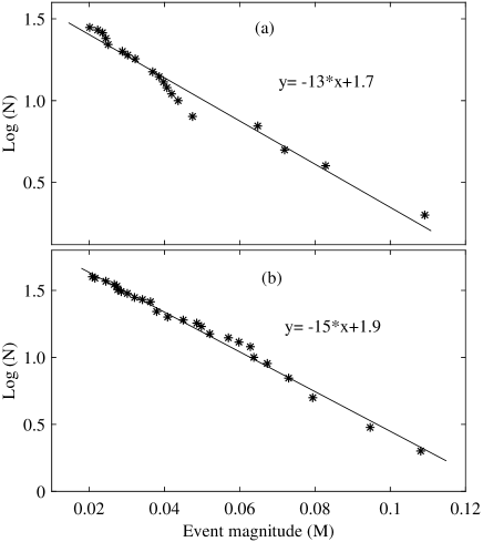
Fig. 5 (a) and (b) show the typical plot of $\log(N)$ versus $\log(M)$ of S&P 500 index and Amazon Inc., respectively during the financial-crisis-2008. The points show the aftershocks with its magnitude, and the straight line represents the best fit of the aftershock sequence. We clearly see that the number of aftershocks with high magnitude is very low, and the number of aftershocks with low magnitude is very high which can be observed from the cluster of points formed around low magnitude region. This shows that the aftershocks with high magnitude are rare and aftershocks with low magnitude occurs frequently until the market fully recovers from the shock. The obtained value of $\alpha$ and $\beta$ of Eqn.1 during the financial crisis for S&P 500 are 1.7 and 13.0 and for Amazon Inc. are 1.9 and 15.0, respectively. The absolute value of $\beta$ in Fig. 5 (a) is less than Fig. 5 (b) which indicates the later will experience large aftershocks with high volatility whereas the former will take longer time to recover. This is generally true as indices fall and recover slowly compared to individual stocks. The values of $\alpha$ and $\beta$ are calculated for all the 51 stocks which is shown in Table 1. Adjusted $R^{2}$ and P-value are also calculated for the same. From the figure and the values of $R^{2}$ and P-value it is clear that aftershocks sequence of S&P 500 and Amazon Inc. follow the GR power law during the financial-crisis-2008. Similar results have been found for the rest of the 49 companies for financial-crisis-2008. Detailed analysis of all the indices and companies are given in Table 1.

Figure 6: It represents the plot between cumulative number of events ($N$) and the corresponding magnitude ($M$) of (a) S&P500 index and (b) Amazon Inc., respectively during the COVID-19.

IV.3 The COVID-19 pandemic

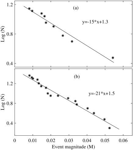
Fig. 6 (a) and (b) show the plots of $\log(N)$ vs. $\log(M)$ of S&P 500 index and Amazon Inc., respectively during the ongoing COVID-19 pandemic. The straight line represents the best fit and the values of $\alpha$ and $\beta$ for S&P 500 are 1.3 and 15.0 and for Amazon Inc. are 1.5 and 21.0, respectively. It is observed that the absolute value of $\beta$ in Fig. 6 (a) is less than Fig. 6 (b). This imply that the Amazon Inc. has higher volatility and S&P 500 index will have a longer turbulent period. It is also clear from Fig. 6(a) and (b) that the aftershock sequence of S&P 500 and Amazon Inc. follow the GR power law during this ongoing pandemic. We have carried out the analysis for all the 51 companies and indices and found that these indices and companies follow the GR power law. Detailed analysis of all the indices and companies are given in Table 1.

It is interesting to note that for the COVID-19 pandemic, there is no cluster of points in the low magnitude region as observed in the Fig. 5 (a) and (b), and a gap between the highest magnitude aftershock and its next aftershock is observed in Fig. 6 (a). These observations give us a strong indication that more aftershocks with low magnitude can be anticipated in the near future due to the ongoing COVID-19 pandemic. The gap seen in high magnitude region in Fig. 6 (a) shows the possibility of high-magnitude aftershocks in the near future.

The results show that the absolute $\beta$ is greater for the COVID-19 pandemic than the financial-crisis-2008. This implies that the stock market was highly volatile during the COVID-19 pandemic but its recovery was also swift. Whereas, the financial-crisis-2008 had a much severe impact on the stock market in terms of duration of its impact which lasted for few years. The difference in $\beta$ value indicates that the effect of the COVID-19 pandemic will not last longer than the financial-crisis-2008.

Figure 7: It represent the mainshock and the aftershocks of S&P 500 index during (a) the financial-crisis-2008 and (b) the COVID-19 pandemic, respectively.

IV.4 Analysis of temporal variance and Inter-occurrence time of aftershocks

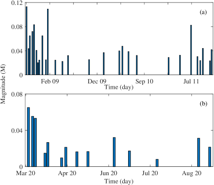
The temporal variance of the aftershock sequence is presented in Fig. 7 (a) and (b) of S&P 500 during the financial-crisis-2008 and the COVID-19 pandemic, respectively. They show that the number of aftershocks per unit time does not decay with time. Sometimes the number of aftershocks per unit time increases and hence does not follow the Omori law. This finding is in contradiction to the previous studies Siokis (2012); Selçuk (2004); Petersen et al. (2010). Our finding is consistent with the statistics of the mainshock and aftershocks in stock price as explained below.

After a major crash, the market recovers for a certain period, but due to some negative perturbation, stressed condition of economy and fear of investors lead to smaller crashes. During the stressed period of the market recovery, it is observed that the number of aftershocks per unit time increases significantly at the later period of market recovery. Hence, it is unlikely to follow Omori law during the market recovery after a major crash. The studies shown in Ref. Siokis (2012); Selçuk (2004); Petersen et al. (2010) on the decay of aftershocks with time that holds Omori law may be incomplete due to the erroneous definition of the mainshock, aftershocks and duration of influence that is discussed in Sec.I.

Figure 8: It represents the plot between (a) mean occurrence time ($R$) and threshold ($Q$) and, (b) the distribution $P_{Q}(r)$ and interoccurence time ($r$), for S&P 500, Amazon Inc., BSE SENSEX and TCS Ltd.

Figure 9: It represents the plot between the distribution $P(\tau_{i})$ and occurrence time $(\tau_{i})$ of S&P 500 index for different mean interoccurence time ($R$)

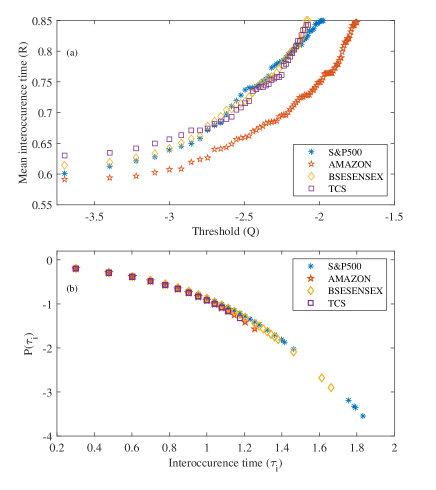
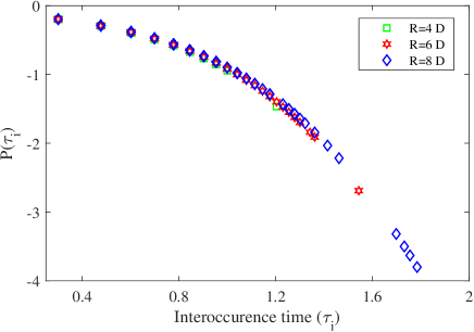
To study the characteristics of the inter-occurrence time($\tau_{i}$) between the aftershocks above a threshold ($Q$), we analyze the distribution P($\tau_{i}$). We found that for all the stocks, the $P(\tau_{i})$ follows the generalized Pareto distribution Reiss, Thomas, and Reiss (1997), i.e., $\displaystyle~{}P(\tau_{i})\propto\frac{1}{\{1+\lambda(q-1)\tau_{i}\}^{\frac{1}{(q-1)}}}$, where $\lambda$ and $q$ are constants. $q$ can be estimated using relation $\displaystyle~{}q=1+q_{0}+\ln{\frac{R}{2}},$ where $R$ is the mean inter-occurence time. Fig. 8 (a) shows the plot of $R$ vs. $Q$ for S&P 500 index, Amazon Inc., BSE SENSEX index and TCS Ltd. during the financial-crisis-2008. The plot shows that the value of $R$ increases slowly at low value of $Q$ but for higher $Q$ values $R$ increases by power law. Fig. 8 (b) shows the plot of $P(\tau_{i})$ vs. $\tau_{i}$ for S&P 500 index, Amazon Inc., BSE SENSEX index and TCS Ltd. Earlier, we had considered any fall that is greater than 7% of the main shock as an aftershock. Hence, in this analysis we have given a maximum $Q$ of 7% of the mainshock for all the stocks and indices. We have obtained the value of $R$ for all the stocks. As all the $R^{\prime}s$ are in very close range, the variation in $P(\tau_{i})$ with respect to $R$ is negligible. Fig 9 shows the plot of $P(\tau_{i})$ vs. $(\tau_{i})$ of S&P 500 index for different $R$ i.e., 4, 6, and 8 trading days which is seen to overlap with each other.

V Conclusion

This paper draws the limitation of the previous works with respect to their interpretation of crash and duration of effect of the mainshock. The statistical nature of the aftershock sequence after major stock market crashes for the 1987 crash, the financial-crisis-2008 and the ongoing COVID-19 pandemic are analysed using the new definition of crash. The analysis is carried out for 51 stocks and indices, considering the mainshock or aftershock as a cumulative consecutive fall of the stock price. The duration of influence of the mainshock is obtained by the 3-point structural break method. The mainshock and aftershocks follow the Gutenberg-Richter power law. We found that in the 1987 crash and the financial-crisis-2008 there are a dense cluster of aftershocks in the low magnitude region. This indicates that aftershock of low magnitude occurs more frequently rather than high magnitude aftershock.

The analysis shows that in the ongoing COVID-19 event, the number of aftershocks in the low-magnitude region is less, and there is a gap in the high-magnitude region. These results indicate that few more aftershocks with smaller amplitudes may be anticipated in the near future during this ongoing pandemic till the pandemic is completely eliminated. However, the probability of an aftershock with a large magnitude during the ongoing COVID-19 pandemic is very less as it is no longer a novel risk to the market. On comparison of the $\beta$ values between the COVID-19 and the financial-crisis-2008, we conclude that the effect of the COVID-19 will not last as long as the financial-crisis-2008. The analysis shows that the number of aftershocks does not necessarily decay with time, and hence, does not obey Omori’s power law. However, inter-occurence-time of the aftershocks follows the generalized pareto distribution.

Our finding is also consistent with the psychology of the investors that when the unique crisis becomes known, the market does not react too irrationally as it did initially, and hence subsequent crashes becomes relatively smaller. When smaller crashes happen during the recovery period, investors need not be worried of such smaller crashes as these crashes will be recovered very quickly. Further, these smaller crashes give the investors opportunities to enter in the stock market. The analysis may help investors make rational investment decisions during the stressed period after a major market crash.

References

- Sornette (2017) D. Sornette, Why stock markets crash: critical events in complex financial systems, Vol. 49 (Princeton University Press, 2017).
- McNamara et al. (2015) D. E. McNamara, H. M. Benz, R. B. Herrmann, E. A. Bergman, P. Earle, A. Holland, R. Baldwin, and A. Gassner, “Earthquake hypocenters and focal mechanisms in central oklahoma reveal a complex system of reactivated subsurface strike-slip faulting,” Geophysical Research Letters 42, 2742–2749 (2015).
- Sarlis et al. (2018) N. V. Sarlis, E. S. Skordas, P. A. Varotsos, A. Ramírez-Rojas, and E. L. Flores-Márquez, “Natural time analysis: On the deadly mexico m8. 2 earthquake on 7 september 2017,” Physica A: Statistical Mechanics and its Applications 506, 625–634 (2018).
- Pisarenko and Sornette (2003) V. Pisarenko and D. Sornette, “Characterization of the frequency of extreme earthquake events by the generalized pareto distribution,” pure and applied geophysics 160, 2343–2364 (2003).
- Nguyen, Bhatti, and Henry (2017) C. Nguyen, M. I. Bhatti, and D. Henry, “Are vietnam and chinese stock markets out of the us contagion effect in extreme events?” Physica A: Statistical Mechanics and its Applications 480, 10–21 (2017).
- Piccoli et al. (2017) P. Piccoli, M. Chaudhury, A. Souza, and W. V. da Silva, “Stock overreaction to extreme market events,” The North American Journal of Economics and Finance 41, 97–111 (2017).
- Zhang et al. (2009) X. Zhang, L. Yu, S. Wang, and K. K. Lai, “Estimating the impact of extreme events on crude oil price: An emd-based event analysis method,” Energy Economics 31, 768–778 (2009).
- Sornette and Johansen (1998) D. Sornette and A. Johansen, “A hierarchical model of financial crashes,” Physica A: Statistical Mechanics and its Applications 261, 581–598 (1998).
- Sornette, Johansen, and Bouchaud (1996) D. Sornette, A. Johansen, and J.-P. Bouchaud, “Stock market crashes, precursors and replicas,” Journal de Physique I 6, 167–175 (1996).
- Mahata et al. (2021a) A. Mahata, A. Rai, M. Nurujjaman, O. Prakash, and D. Prasad Bal, “Characteristics of 2020 stock market crash: The covid-19 induced extreme event,” Chaos: An Interdisciplinary Journal of Nonlinear Science 31, 053115 (2021a).
- Abe and Suzuki (2004) S. Abe and N. Suzuki, “Aging and scaling of earthquake aftershocks,” Physica A: Statistical Mechanics and its Applications 332, 533–538 (2004).
- Siokis (2012) F. M. Siokis, “Stock market dynamics: Before and after stock market crashes,” Physica A: Statistical Mechanics and its Applications 391, 1315–1322 (2012).
- Bak et al. (2002) P. Bak, K. Christensen, L. Danon, and T. Scanlon, “Unified scaling law for earthquakes,” Physical Review Letters 88, 178501 (2002).
- Bai and Zhu (2010) M.-Y. Bai and H.-B. Zhu, “Power law and multiscaling properties of the chinese stock market,” Physica A: Statistical Mechanics and its Applications 389, 1883–1890 (2010).
- Gabaix et al. (2007) X. Gabaix, P. Gopikrishnan, V. Plerou, and E. Stanley, “A unified econophysics explanation for the power-law exponents of stock market activity,” Physica A: Statistical Mechanics and its Applications 382, 81–88 (2007).
- Selçuk (2004) F. Selçuk, “Financial earthquakes, aftershocks and scaling in emerging stock markets,” Physica A: Statistical Mechanics and its Applications 333, 306–316 (2004).
- Kapopoulos and Siokis (2005) P. Kapopoulos and F. Siokis, “Stock market crashes and dynamics of aftershocks,” Economics Letters 89, 48–54 (2005).
- Albuquerque et al. (2020) R. Albuquerque, Y. Koskinen, S. Yang, and C. Zhang, “Resiliency of environmental and social stocks: an analysis of the exogenous covid-19 market crash,” The Review of Corporate Finance Studies 9, 593–621 (2020).
- Mazur, Dang, and Vega (2020) M. Mazur, M. Dang, and M. Vega, “Covid-19 and the march 2020 stock market crash. evidence from s&p1500,” Finance Research Letters , 101690 (2020).
- Lyócsa et al. (2020) Š. Lyócsa, E. Baumöhl, T. Vỳrost, and P. Molnár, “Fear of the coronavirus and the stock markets,” Finance research letters 36, 101735 (2020).
- Baker et al. (2020) S. R. Baker, N. Bloom, S. J. Davis, K. J. Kost, M. C. Sammon, and T. Viratyosin, “The unprecedented stock market impact of covid-19,” Tech. Rep. (National Bureau of Economic Research, 2020).
- Wang et al. (2009) J. Wang, G. Meric, Z. Liu, and I. Meric, “Stock market crashes, firm characteristics, and stock returns,” Journal of Banking & Finance 33, 1563–1574 (2009).
- Barlevy and Veronesi (2003) G. Barlevy and P. Veronesi, “Rational panics and stock market crashes,” Journal of Economic Theory 110, 234–263 (2003).
- Chiang and Zheng (2010) T. C. Chiang and D. Zheng, “An empirical analysis of herd behavior in global stock markets,” Journal of Banking & Finance 34, 1911–1921 (2010).
- Tan et al. (2008) L. Tan, T. C. Chiang, J. R. Mason, and E. Nelling, “Herding behavior in chinese stock markets: An examination of a and b shares,” Pacific-Basin Finance Journal 16, 61–77 (2008).
- White (1990) E. N. White, “The stock market boom and crash of 1929 revisited,” Journal of Economic perspectives 4, 67–83 (1990).
- Choudhry (1996) T. Choudhry, “Stock market volatility and the crash of 1987: evidence from six emerging markets,” Journal of International money and Finance 15, 969–981 (1996).
- Carlson (2007) M. A. Carlson, “A brief history of the 1987 stock market crash with a discussion of the federal reserve response,” (2007).
- Grant (1990) J. L. Grant, “Stock return volatility during the crash of 1987,” Journal of Portfolio Management 16, 69 (1990).
- Sornette and Johansen (1997) D. Sornette and A. Johansen, “Large financial crashes,” Physica A: Statistical Mechanics and its Applications 245, 411–422 (1997).
- Mahata et al. (2021b) A. Mahata, A. Rai, M. Nurujjaman, and O. Prakash, “Modeling and analysis of the effect of covid-19 on the stock price: V and l-shape recovery,” Physica A: Statistical Mechanics and its Applications 574, 126008 (2021b).
- Netter and Mitchell (1989) J. M. Netter and M. L. Mitchell, “Stock-repurchase announcements and insider transactions after the october 1987 stock market crash,” Financial Management , 84–96 (1989).
- Hong and Stein (2003) H. Hong and J. C. Stein, “Differences of opinion, short-sales constraints, and market crashes,” The Review of Financial Studies 16, 487–525 (2003).
- Gopikrishnan et al. (2000) P. Gopikrishnan, V. Plerou, X. Gabaix, and H. E. Stanley, “Statistical properties of share volume traded in financial markets,” Physical review e 62, R4493 (2000).
- Oh et al. (2011) G. Oh, C. Eom, F. Wang, W.-S. Jung, H. E. Stanley, and S. Kim, “Statistical properties of cross-correlation in the korean stock market,” The European Physical Journal B 79, 55–60 (2011).
- Liu et al. (1999) Y. Liu, P. Gopikrishnan, H. E. Stanley, et al., “Statistical properties of the volatility of price fluctuations,” Physical review e 60, 1390 (1999).
- Mantegna and Stanley (1997) R. N. Mantegna and H. E. Stanley, “Stock market dynamics and turbulence: parallel analysis of fluctuation phenomena,” Physica A: Statistical Mechanics and its Applications 239, 255–266 (1997).
- Cont (2001) R. Cont, “Empirical properties of asset returns: stylized facts and statistical issues,” (2001).
- Restocchi, McGroarty, and Gerding (2019) V. Restocchi, F. McGroarty, and E. Gerding, “Statistical properties of volume and calendar effects in prediction markets,” Physica A: Statistical Mechanics and its Applications 523, 1150–1160 (2019).
- Da Cunha and da Silva (2020) C. Da Cunha and R. da Silva, “Relevant stylized facts about bitcoin: Fluctuations, first return probability, and natural phenomena,” Physica A: Statistical Mechanics and its Applications 550, 124155 (2020).
- Noh (2000) J. D. Noh, “Model for correlations in stock markets,” Physical Review E 61, 5981 (2000).
- Hamao, Masulis, and Ng (1990) Y. Hamao, R. W. Masulis, and V. Ng, “Correlations in price changes and volatility across international stock markets,” The review of financial studies 3, 281–307 (1990).
- Wang, Shang, and Ge (2012) J. Wang, P. Shang, and W. Ge, “Multifractal cross-correlation analysis based on statistical moments,” Fractals 20, 271–279 (2012).
- Turiel and Pérez-Vicente (2003) A. Turiel and C. J. Pérez-Vicente, “Multifractal geometry in stock market time series,” Physica A: Statistical Mechanics and its Applications 322, 629–649 (2003).
- Potirakis, Zitis, and Eftaxias (2013) S. M. Potirakis, P. I. Zitis, and K. Eftaxias, “Dynamical analogy between economical crisis and earthquake dynamics within the nonextensive statistical mechanics framework,” Physica A: Statistical Mechanics and its Applications 392, 2940–2954 (2013).
- Petersen et al. (2010) A. M. Petersen, F. Wang, S. Havlin, and H. E. Stanley, “Market dynamics immediately before and after financial shocks: Quantifying the omori, productivity, and bath laws,” Physical Review E 82, 036114 (2010).
- Lillo and Mantegna (2003) F. Lillo and R. N. Mantegna, “Power-law relaxation in a complex system: Omori law after a financial market crash,” Physical Review E 68, 016119 (2003).
- Mu and Zhou (2008) G.-H. Mu and W.-X. Zhou, “Relaxation dynamics of aftershocks after large volatility shocks in the ssec index,” Physica A: Statistical Mechanics and its Applications 387, 5211–5218 (2008).
- Gresnigt, Kole, and Franses (2015) F. Gresnigt, E. Kole, and P. H. Franses, “Interpreting financial market crashes as earthquakes: A new early warning system for medium term crashes,” Journal of Banking & Finance 56, 123–139 (2015).
- Bai and Perron (1998) J. Bai and P. Perron, “Estimating and testing linear models with multiple structural changes,” Econometrica , 47–78 (1998).
- Bai and Perron (2003) J. Bai and P. Perron, “Computation and analysis of multiple structural change models,” Journal of applied econometrics 18, 1–22 (2003).
- Clauset, Shalizi, and Newman (2009) A. Clauset, C. R. Shalizi, and M. E. Newman, “Power-law distributions in empirical data,” SIAM review 51, 661–703 (2009).
- Taleghani, Salehi, and Shakibaiee (2019) F. Taleghani, M. Salehi, and A. Shakibaiee, “An analysis of the repeated financial earthquakes,” Advances in Mathematical Finance and Applications 4, 59–76 (2019).
- Sornette and Sornette (1999) D. Sornette and A. Sornette, “General theory of the modified gutenberg-richter law for large seismic moments,” Bulletin of the Seismological Society of America 89, 1121–1130 (1999).
- Gutenberg and Richter (1944) B. Gutenberg and C. F. Richter, “Frequency of earthquakes in california,” Bulletin of the Seismological Society of America 34, 185–188 (1944).
- Chowdhury et al. (2017) S. Chowdhury, A. Deb, M. Nurujjaman, and C. Barman, “Identification of pre-seismic anomalies of soil radon-222 signal using hilbert–huang transform,” Natural Hazards 87, 1587–1606 (2017).
- Huang et al. (1998) N. E. Huang, Z. Shen, S. R. Long, M. C. Wu, H. H. Shih, Q. Zheng, N.-C. Yen, C. C. Tung, and H. H. Liu, “The empirical mode decomposition and the hilbert spectrum for nonlinear and non-stationary time series analysis,” Proceedings of the Royal Society of London. Series A: mathematical, physical and engineering sciences 454, 903–995 (1998).
- Mahata, Bal, and Nurujjaman (2020) A. Mahata, D. P. Bal, and M. Nurujjaman, “Identification of short-term and long-term time scales in stock markets and effect of structural break,” Physica A: Statistical Mechanics and its Applications 545, 123612 (2020).
- (59) https://in.finance.yahoo.com/.
- Reiss, Thomas, and Reiss (1997) R.-D. Reiss, M. Thomas, and R. Reiss, Statistical analysis of extreme values, Vol. 2 (Springer, 1997).