MFES-HB: Efficient Hyperband with Multi-Fidelity Quality Measurements

Abstract

Hyperparameter optimization (HPO) is a fundamental problem in automatic machine learning (AutoML). However, due to the expensive evaluation cost of models (e.g., training deep learning models or training models on large datasets), vanilla Bayesian optimization (BO) is typically computationally infeasible. To alleviate this issue, Hyperband (HB) utilizes the early stopping mechanism to speed up configuration evaluations by terminating those badly-performing configurations in advance. This leads to two kinds of quality measurements: (1) many low-fidelity measurements for configurations that get early-stopped, and (2) few high-fidelity measurements for configurations that are evaluated without being early stopped. The state-of-the-art HB-style method, BOHB, aims to combine the benefits of both BO and HB. Instead of sampling configurations randomly in HB, BOHB samples configurations based on a BO surrogate model, which is constructed with the high-fidelity measurements only. However, the scarcity of high-fidelity measurements greatly hampers the efficiency of BO to guide the configuration search.

In this paper, we present MFES-HB, an efficient Hyperband method that is capable of utilizing both the high-fidelity and low-fidelity measurements to accelerate the convergence of HPO tasks. Designing MFES-HB is not trivial as the low-fidelity measurements can be biased yet informative to guide the configuration search. Thus we propose to build a Multi-Fidelity Ensemble Surrogate (MFES) based on the generalized Product of Experts framework, which can integrate useful information from multi-fidelity measurements effectively. The empirical studies on the real-world AutoML tasks demonstrate that MFES-HB can achieve $3.3-8.9\times$ speedups over the state-of-the-art approach — BOHB.

Introduction

The performance of Machine Learning (ML) models heavily depends on the specific choice of hyperparameter configurations. As a result, automatically tuning the hyperparameters has attracted lots of interest from both academia and industry, and has become an indispensable component in modern AutoML systems (Hutter, Kotthoff, and Vanschoren 2018; Yao et al. 2018; Zöller and Huber 2019). Hyperparameter optimization (HPO) is often a computationally-intensive process as one often needs to try hyperparameter configurations iteratively, and evaluate each configuration by training and validating the corresponding ML model. However, for ML models that are computationally expensive to train (e.g., deep learning models or models trained on large datasets), vanilla Bayesian optimization (BO) (Hutter, Hoos, and Leyton-Brown 2011; Bergstra et al. 2011; Snoek, Larochelle, and Adams 2012), one of the most prevailing frameworks in solving the HPO problem, suffers from the low-efficiency issue due to insufficient configuration evaluations within a limited budget.

Instead, Hyperband (HB) (Li et al. 2018) is a popular alternative, which uses the early stopping strategy to speed up configuration evaluation. In HB, the system dynamically allocates resources to a set of configurations drawn from a uniform distribution, and uses successive halving (Jamieson and Talwalkar 2016) to early stop the poorly-performing configurations after measuring their quality periodically. Among many efforts to improve Hyperband (Klein et al. 2017b; Falkner, Klein, and Hutter 2018), BOHB (Falkner, Klein, and Hutter 2018) combines the benefits from both Hyperband and traditional BO. It replaces the configuration sampling procedure in HB from the uniform distribution to a BO surrogate model —TPE (Bergstra et al. 2011), which is fitted on those quality measurements obtained from the evaluations without being early stopped.

Due to the successive halving strategy of HB, most configuration evaluations end up being early stopped by the system, thus creating two kinds of quality measurements: (1) many low-fidelity quality measurements of these early-stopped configurations, and (2) few high-fidelity quality measurements of configurations that are evaluated with complete training resources. One fundamental limitation of BOHB lies in the fact that the BO component only utilizes the few high-fidelity measurements to sample configurations, which are insufficient to train a BO surrogate that models the objective function in HPO well. Consequently, like vanilla BO, sampling configurations in BOHB also suffers from the low-efficiency issue. Can we also take advantage of the low-fidelity quality measurements, which are ignored by the existing methods, to further speed up the Hyperband-style methods? In this paper, our goal is to investigate a new Hyperband-style method, which is capable of utilizing the multi-fidelity quality measurements: both the high-fidelity measurements and the low-fidelity measurements, to accelerate the HPO process.

(Opportunities and Challenges) Taking advantage of the multi-fidelity quality measurements poses unique opportunities and challenges. Intuitively, numerous low-fidelity measurements are obtained from the early-stopped evaluations, which can boost the total number of measurements that BO can use. The low-fidelity measurements obtained with partial training resources yield a biased surrogate of the high-fidelity quality measurements. Nevertheless, due to the relevancy between early-stopped evaluations and complete evaluations, they can still reveal some useful information about the objective function. Therefore, there is great potential for utilizing the low-fidelity measurements to accelerate HPO. However, if we cannot balance the benefits and biases from the low-fidelity measurements well, we might be misled by the harmful information towards a wrong objective function.

In this paper, we propose MFES-HB, an efficient Hyperband method, which is capable of utilizing the planetary unexploited multi-fidelity measurements to significantly accelerate the convergence of configuration search. To utilize the multi-fidelity measurements without introducing the biases from the low-fidelity measurements, we first train multiple base surrogates on these measurements grouped by their fidelities. Then we propose the Multi-Fidelity Ensemble Surrogate (MFES) that is used in the BO framework to sample configurations. Concretely, to make the best usage of those biased yet informative low-fidelity measurements, MFES uses the generalized Product of Experts (gPoE) (Cao and Fleet 2014) to combine these base surrogates, and the contribution of each base surrogate to MFES can be adjusted based on their performance when approximating the objective function. Therefore, the heterogeneous information among multi-fidelity measurements could be automatically extracted by MFES in a reliable yet efficient way. The empirical studies on the real-world HPO tasks demonstrate the superiority of the proposed method over competitive baselines. MFES-HB can achieve an order of magnitude speedups compared with Hyperband, and $3.3-8.9\times$ speedups over the state-of-the-art method — BOHB.

Related Work

Bayesian Optimization (BO). Machine learning (ML) has made great strides in many application areas, e.g., recommendation, computer vision, etc (Goodfellow, Bengio, and Courville 2016; He et al. 2017; Jiang et al. 2017; Ma et al. 2019; Wu et al. 2020; Zhang et al. 2020). BO has been successfully applied to tune the hyperparameters of ML models. The main idea of BO is to use a probabilistic surrogate model $M:p_{M}(f|\bm{x})$ to describe the relationship between a hyperparameter configuration $\bm{x}$ and its performance $f(\bm{x})$ (e.g., validation error), and then utilizes this surrogate to guide the configuration search (See more details about BO in Section 3). Spearmint (Snoek, Larochelle, and Adams 2012) uses Gaussian process (GP) to model $p_{M}(f|\bm{x})$ as a Gaussian distribution, and TPE (Bergstra et al. 2011) employs a tree-structured Parzen density estimators to model $p_{M}(f|\bm{x})$. Lastly, SMAC (Hutter, Hoos, and Leyton-Brown 2011) adopts a modified random forest to yield an uncertain estimate of $f(\bm{x})$. An empirical evaluation of the three methods (Eggensperger et al. 2013) shows that SMAC performs the best on the benchmarks with high-dimensional and complex hyperparameter space that includes categorical and conditional hyperparameters, closely followed by TPE. Spearmint only works well with low-dimensional continuous hyperparameters, and cannot apply to complex configuration space easily.

Early stopping mechanism that stops the evaluations of poorly-performing configurations early, has been discussed in many methods (Swersky, Snoek, and Adams 2014; Domhan, Springenberg, and Hutter 2015; Baker et al. 2017; Klein et al. 2017b; Falkner, Klein, and Hutter 2018; Wang, Xu, and Wang 2018; Bertrand et al. 2017; Dai et al. 2019), including Hyperband (HB) (Li et al. 2018) and BOHB (Falkner, Klein, and Hutter 2018). In Section 3, we will describe HB in more detail. Among them, LCNET-HB (Klein et al. 2017b) utilizes the LCNET that predicts the learning curve of configurations to sample configurations in HB. In this paper, we explore to use the multi-fidelity quality measurements in the BO framework to further accelerate the HB-style methods.

Multi-fidelity Optimization methods exploit the low-fidelity measurements about the objective function $f$ to guide the search for the optimum of $f$, by conducting cheap low-fidelity evaluations proactively, instead of early stopping (Swersky, Snoek, and Adams 2013; Klein et al. 2017a; Kandasamy et al. 2017; Poloczek, Wang, and Frazier 2017; Hu et al. 2019; Sen, Kandasamy, and Shakkottai 2018; Wu et al. 2019b, a; Takeno et al. 2020). For instance, FABOLAS (Klein et al. 2017a) and TSE (Hu et al. 2019) evaluate configurations on subsets of the training data and use the generated low-fidelity measurements to infer the quality on the full training set.

Transfer Learning methods for HPO aim to take advantage of auxiliary knowledge/information acquired from the past HPO tasks (source problems) to achieve a faster convergence for the current HPO task (target problem) (Bardenet et al. 2013; Yogatama and Mann 2014; Schilling et al. 2015; Wistuba, Schilling, and Schmidt-Thieme 2016; Schilling, Wistuba, and Schmidt-Thieme 2016; Golovin et al. 2017; Feurer, Letham, and Bakshy 2018). While sharing a similar idea, here we investigate to speed up HB-style methods by using the multi-fidelity measurements from the current HPO task, instead of the measurements from past similar tasks. Thus, our work is inspired by, but orthogonal to the transfer learning-related methods.

Algorithm 1 Pseudo code for Hyperband.

Input: maximum amount of resource that can be allocated to a single hyperparameter configuration $R$, the discard proportion $\eta$, and hyperparameter space $\mathcal{X}$.

1:  Initialize $s_{max}=\lfloor log_{\eta}(R)\rfloor$, $B=(s_{max}+1)R$.

2:  for $s\in\{s_{max},s_{max}-1,...,0\}$ do

3:     $n_{1}=\lceil\frac{B}{R}\frac{\eta^{s}}{s+1}\rceil$, $r_{1}=R\eta^{-s}$.

4:     sample $n_{1}$ configurations from $\mathcal{X}$ randomly.

5:     execute the SH with the $n_{1}$ configurations and $r_{1}$ as input (the inner loop).

6:  end for

7:  return the configuration with the best evaluation result.

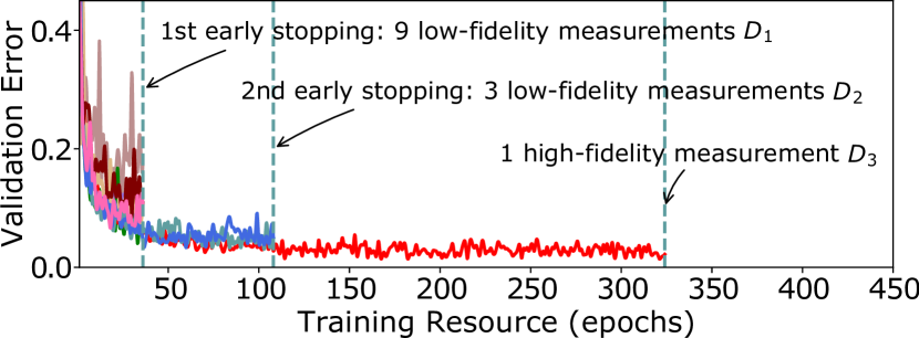
Figure 1: Successive halving process (the inner loop of HB) in tuning a neural network where $n_{1}=9$, $r_{1}=1$, $R=9$, and $\eta=3$; one unit of resource corresponds to 36 epochs. First, 9 configurations are evaluated with 1 unit of resource. Then the top 3rd configurations continue their evaluations with 3 units of resources. Finally, only one configuration is evaluated with the maximum training resource $R$.

	$s=4$			$s=3$			$s=2$			$s=1$			$s=0$
$i$	$n_{i}$		$r_{i}$	$n_{i}$		$r_{i}$	$n_{i}$		$r_{i}$	$n_{i}$		$r_{i}$	$n_{i}$		$r_{i}$
$1$	$81$		$1$	$27$		$3$	$9$		$9$	$6$		$27$	$\bm{5}$		$81$
$2$	$27$		$3$	$9$		$9$	$3$		$27$	$\bm{2}$		$81$
$3$	$9$		$9$	$3$		$27$	$\bm{1}$		$81$
$4$	$3$		$27$	$\bm{1}$		$81$
$5$	$\bm{1}$		$81$

Table 1: The values of $n_{i}$ and $r_{i}$ in the HB evaluations. Here $R=81$ and $\eta=3$. Each column displays an inner loop (SH process). The pair ($n_{i}$, $r_{i}$) in each cell means there are $n_{i}$ configuration evaluations with $r_{i}$ units of training resources.

Bayesian Hyperparameter Optimization and Hyperband

We model the loss $f(\bm{x})$ (e.g., validation error), which reflects the quality of an ML algorithm with the given hyperparameter configuration $\bm{x}\in\mathcal{X}$, as a black-box optimization problem. The goal of hyperparameter optimization (HPO) is to find $\arg\min_{\bm{x}\in\mathcal{X}}f(\bm{x})$, where the only mode of interaction with the objective function $f$ is to evaluate the given configuration $\bm{x}$. Due to the randomness of most ML algorithms, we assume that $f(\bm{x})$ cannot be observed directly but rather through noisy observation $y=f(\bm{x})+\epsilon$, with $\epsilon\sim\mathcal{N}(0,\sigma^{2})$. We now introduce two methods for solving this black-box optimization problem in more detail: Bayesian optimization and Hyperband, which are the basic ingredients in MFES-HB.

Bayesian Optimization

The main idea of Bayesian optimization (BO) is as follows. Since evaluating the objective function $f$ for a given configuration $\bm{x}$ is very expensive, it approximates $f$ using a probabilistic surrogate model $M:p(f|D)$ that is much cheaper to evaluate. Given a configuration $\bm{x}$, the surrogate model $M$ outputs the posterior predictive distribution at $\bm{x}$, that is, $f(\bm{x})\sim\mathcal{N}(\mu_{M}(\bm{x}),\sigma^{2}_{M}(\bm{x}))$. In the $n^{th}$ iteration, BO methods iterate the following three steps: (1) use the surrogate model $M$ to select a configuration that maximizes the acquisition function $\bm{x}_{n}=\arg\max_{\bm{x}\in\mathcal{X}}a(\bm{x};M)$, where the acquisition function is used to balance the exploration and exploitation; (2) evaluate the configuration $\bm{x}_{n}$ to get its performance $y_{n}=f(\bm{x}_{n})+\epsilon$ with $\epsilon\sim\mathcal{N}(0,\sigma^{2})$; (3) add this measurement $(\bm{x}_{n},y_{n})$ to the observed quality measurements $D=\{(\bm{x}_{1},y_{1}),...,(\bm{x}_{n-1},y_{n-1})\}$, and refit the surrogate model on the augmented $D$. Expected improvement (EI) (Jones, Schonlau, and Welch 1998) is a common acquisition function:

$$a(\bm{x};M)=\int_{-\infty}^{\infty}\max(y^{\ast}-y,0)p_{M}(y|\bm{x})dy,$$ (1)

where $y^{\ast}$ is the best observed performance in $D$, i.e., $y^{\ast}=\min\{y_{1},...,y_{n}\}$, and $M$ is the probabilistic surrogate model. By maximizing this EI function $a(\bm{x};M)$ over the hyperparameter space $\mathcal{X}$, BO methods can find a configuration with the largest EI value to evaluate in each iteration.

Low-efficiency issue One fundamental challenge of BO is that, for models that are computationally expensive to train , each complete evaluation of configuration $\bm{x}$ often takes a significant amount of time. Given a limited budget, few measurements can be obtained, and it is insufficient for BO methods to fit a surrogate that approximates $f$ well. In this case, BO methods fail to converge to the optimal solution quickly (Wang et al. 2013; Li et al. 2020).

Hyperband

To accommodate the above issue of BO, Hyperband (HB) (Li et al. 2018) proposes to speed up configuration evaluations by early stopping the badly-performing configurations. It has the following two loops:

(1) Inner Loop: successive halving (SH)  Given a kind of training resource (e.g., the number of iterations, the size of the training subset), HB first evaluates $n_{1}$ hyperparameter configurations with the initial $r_{1}$ units of resources, and ranks them by the evaluation performance. Then HB continues the top $\eta^{-1}$ configurations with $\eta$ times larger resources (usually $\eta=3$), that’s, $n_{2}=n_{1}*\eta^{-1}$ and $r_{2}=r_{1}*\eta$, and stops the evaluations of the other configurations in advance. This process repeats until the maximum training resource $R$ is reached, that’s, $r_{i}=R$. We provide an example to illustrate this procedure in Figure 1.

(2) Outer Loop: grid search of $n_{1}$ and $r_{1}$  Given a fixed budget $B$, the values of $n_{1}$ and $r_{1}$ should be carefully chosen because a larger $n_{1}$ with a small initial training resource $r_{1}$ may lead to the elimination of good configurations in SH process by mistake. There is no prior whether we should use a larger $n_{1}$ with a small initial training resource $r_{1}$, or a smaller $n_{1}$ with a larger $r_{1}$. HB addresses this “$n$ versus $B/n$” problem by performing a grid search over feasible values of $n_{1}$ and $r_{1}$ in the outer loop. Algorithm 1 shows the enumeration of $n_{1}$ and $r_{1}$ in Line 3. Table 1 lists the number of evaluations and their corresponding training resources in one iteration of HB. Note that, the HB algorithm can be called multiple times until the HPO budget exhausts.

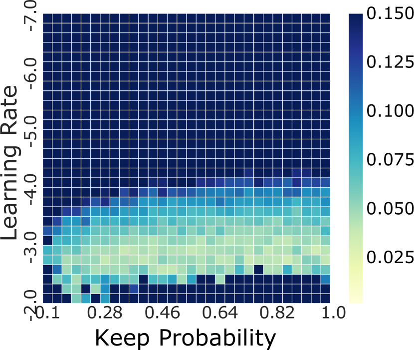
(a) $D_{1}$: $r_{1}=1$

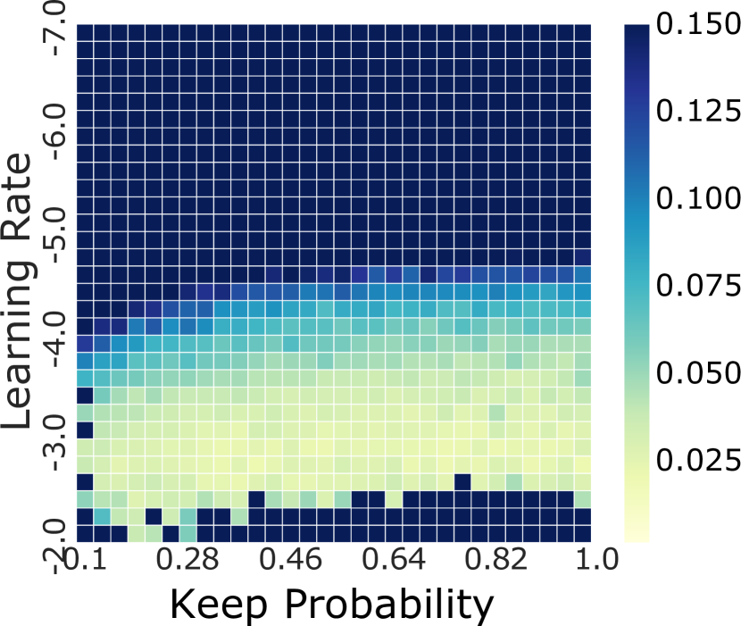
(b) $D_{2}$: $r_{2}=3$

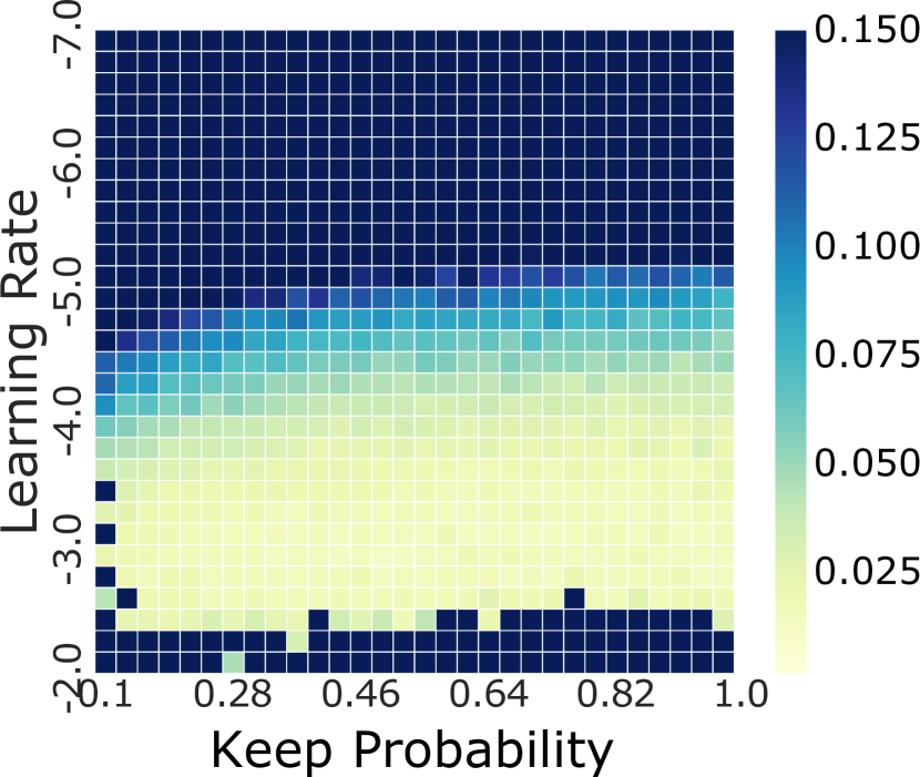
(c) $D_{3}$: $r_{3}=9$

(d) $D_{4}$: $r_{4}=27$

Figure 2: Validation error of 900 LeNet configurations (30 settings of keep probability $\lambda=1-dropout\_value$ in dropout layer and 30 settings of the learning rate $\alpha$ on a base-10 log scale in [-7, -2]) on the MNIST dataset using different training resources $r={1,3,9,27}$. $R=27$, $K=4$, and one unit of resource corresponds to an epoch.

The problem of HB and BOHB. The disadvantage of HB lies in that it samples configurations randomly from the uniform distribution. To improve it, BOHB utilizes a BO component to sample configurations in HB iteration, instead of the uniform distribution. However, BOHB also suffers from the low-efficiency issue due to the scarcity of high-fidelity quality measurements. Consequently, BOHB does not fully unleash the potential for combining BO and HB.

Efficient Hyperband using Multi-Fidelity Quality Measurements

In this section, we introduce MFES-HB, an efficient Hyperband method that can utilize the multi-fidelity quality measurements in the framework of BO to speed up the convergence of configuration search. First, we investigate the characteristics of multi-fidelity measurements, and then describe the proposed Multi-Fidelity Ensemble Surrogate (MFES) that is capable of extracting instrumental information from multi-fidelity measurements effectively.

Multi-fidelity Quality Measurements

According to the number of training resources used by the evaluations in HB, we can categorize the multi-fidelity measurements into $K$ groups: $D_{1},...,D_{K}$, where $K=\lfloor log_{\eta}(R)\rfloor+1$, and typically $K$ is less than $7$. The (quality) measurement ($\bm{x}$, $y$) in each group $D_{i}$ with $i\in[1:K]$ is obtained by evaluating $\bm{x}$ with $r_{i}=\eta^{i-1}$ units of resources. Thus $D_{K}$ denotes the high-fidelity measurements from the evaluations with the maximum training resource $r_{K}=R$, and $D_{1:K-1}$ denote the low-fidelity measurements obtained from the early-stopped evaluations. Then we discuss the characteristics of $D_{1:K}$ from two aspects:

(1) The number of measurements Due to successive halving strategy, the number of measurements in $D_{i}$, i.e., $N_{i}=|D_{i}|$, satisfies that $N_{1}>N_{2}>...>N_{K}$. Here, $N_{i}$ denotes the total number of measurements in each $D_{i}$ with training resource $r_{i}$. Table 1 shows the $N_{i}$s in one iteration of HB, that is, $N_{1}=81$, $N_{2}=54$, $N_{3}=27$, $N_{3}=15$, and $N_{5}=10$.

(2) The fidelities of measurements The high-fidelity measurements, $D_{K}$, consist of the unbiased measurements of the objective function $f$. The other $D_{i}$s, the low-fidelity measurements, are composed of the biased measurements about $f$. The BO surrogate model $M_{i}$, fitted on $D_{i}$ with $i<K$, is to model the objective function $f^{i}$ with training resource $r_{i}$, instead of the true objective function $f=f^{K}$ with the maximum training resource $R$. Although $f^{1:K-1}$ are different from $f$, they have some correlation. As $i$ increases, the surrogate $M_{i}$, learned on the measurements $D_{i}$ with a larger training resource $r_{i}=\eta^{i-1}$, can offer a higher-fidelity approximation to $f$ because $r$ is closer to $R$. Figure 2 provides a brief example to illustrate the diversity of the measurement fidelity in $D_{1:K}$. The quality measurements are visualized as heat maps, where good configurations with low validation errors are marked by the yellow region. By comparing the yellow regions in each sub-figure, we can find that, as $i\in[1:3]$ increases, the measurements in $D_{i}$ with partial training resource $r=\eta^{i-1}$ gradually approach the (unbiased) high-fidelity measurements in $D_{K}$, where $K=4$.

Hence we can conclude that (1) although $D_{1:K-1}$ includes the biased measurements about $f$, it could still reveal some instrumental information to model $f$; (2) the group of quality measurements $D_{i}$ that offers a higher-fidelity approximation to $f$ has a smaller number of measurements $N_{i}$.

The Proposed Algorithm

In MFES-HB, we train $K$ base surrogates on $D_{1:K}$ respectively. (1) $D_{K}$ offers the highest fidelity when modeling $f$, however, the measurements in $D_{K}$ are insufficient to train a BO surrogate that describes $f$ well; (2) although $D_{1:K-1}$ have a much larger number of quality measurements, the low-fidelity measurements in $D_{1:K-1}$ with biases cannot approximate $f$ accurately. Thus none of the base surrogates could approximate $f$ well. Instead, we propose to combine the base surrogates to obtain a more accurate approximation to $f$. However, combining the base surrogates is not trivial as we need to integrate the heterogeneous information behind the base surrogates in a reliable and effective way.

Since the performance $y$ in $D_{i}$s has different numerical ranges, we standardize them by removing the mean and scaling to unit variance respectively. In BO, the uncertainty prediction of the surrogate $M_{i}$ at $\bm{x}$ is a Gaussian, i.e., $f^{i}(\bm{x})\sim\mathcal{N}(\mu_{M_{i}}(\bm{x}),\sigma^{2}_{M_{i}}(\bm{x}))$. For brevity, we use $\mu_{i}(\bm{x})$ and $\sigma^{2}_{i}(\bm{x})$ to denote the mean and variance of predictions from $M_{i}$.

Algorithm 2 Pseudo code of MFES-HB

Input: the hyperparameter space $\mathcal{X}$, the total budget to conduct HPO $B_{hpo}$, maximum amount of resource for a hyperparameter configuration $R$, and the discard proportion $\eta$.
Output: the best configuration found.

1:  initialize: $D_{i}=\varnothing$ with $i\in[1:K]$, $M_{ens}=None$, $s_{max}=\lfloor log_{\eta}(R)\rfloor$, $B=(s_{max}+1)R$.

2:  while budget $B_{hpo}$ does not exhaust. do

3:     for $s\in\{s_{max},s_{max}-1,...,0\}$ do

4:        $n_{1}=\lceil\frac{B}{R}\frac{\eta^{s}}{s+1}\rceil$, $r_{1}=R\eta^{-s}$.

5:        sample $n_{1}$ configurations: $X=Sample(\mathcal{X},M_{ens},n_{1})$.

6:        execute the SH (inner loop) of HB with $X$ and $r_{1}$ as input, and collect the new multi-fidelity quality measurements: $D^{{}^{\prime}}_{1:K}=SH(X,r_{1})$.

7:        $D_{i}=D_{i}\cup D^{{}^{\prime}}_{i}$ with $i=[1:K]$.

8:        update the MFES: $M_{ens}=Build(D_{1:K})$.

9:     end for

10:  end while

11:  return the best configuration $\bm{x}^{\ast}$ in $D_{K}$.

Ensemble Surrogate with gPoE

To fully utilize the biased yet informative low-fidelity measurements, we propose the Multi-Fidelity Ensemble Surrogate (MFES) $M_{ens}$ that can integrate the information from all base surrogates to approximate $f$ effectively. Concretely, a weight $w_{i}$ is assigned to each base surrogate $M_{i}$, which determines the contribution of $M_{i}$ to the ensemble surrogate $M_{ens}$, where $w_{i}\in[0,1]$ and $\sum_{i=1}^{K}w_{i}=1$. The base surrogate $M_{i}$, which offers a more accurate approximation to $f$, should own a larger proportion (larger $w_{i}$) in $M_{ens}$ and vice versa. Thus the weights could reflect the influence of the measurements with different fidelities on $M_{ens}$. Below, we describe the way to combine the base surrogates with weights.

To enable this ensemble surrogate in the BO framework, given a configuration $\bm{x}$, its posterior prediction at $\bm{x}$ should also be a Gaussian, i.e., $f^{ens}(\bm{x})\sim\mathcal{N}(\mu_{ens}(\bm{x}),\sigma^{2}_{ens}(\bm{x})).$ To derive the mean and variance, we need to combine the predictions from base surrogates. The most straightforward solution is to use $\mu_{ens}(\bm{x})=\sum_{i}w_{i}\mu_{i}(\bm{x})$ and $\sigma^{2}_{ens}(\bm{x})=\sum_{i}w_{i}^{2}\sigma_{i}^{2}(\bm{x})$ by assuming that the predictions from base surrogates are independent. However, this assumption is contradictory to the fact that these predictive distributions are correlated as discussed before. Instead, we propose to use the generalized product of experts (gPoE) (Cao and Fleet 2014; Hinton 1999) framework to combine the predictions from $M_{1:K}$s. The predictive mean and variance of the ensemble surrogate $M_{ens}$ at $\bm{x}$ are given by:

$$\mu_{ens}(\bm{x})=(\sum_{i}\mu_{i}(\bm{x})w_{i}\sigma_{i}^{-2}(\bm{x}))\sigma_{ens}^{2}(\bm{x}),$$ (2)

$$\sigma_{ens}^{2}(\bm{x})=(\sum_{i}w_{i}\sigma_{i}^{-2}(\bm{x}))^{-1},$$

where $w_{i}$ is the weight for the $i^{th}$ base surrogate, and it is used to control the influence of individual surrogate $M_{i}$. Using gPoE has the following two advantages: (1) the unified prediction is still a Gaussian; (2) unreliable predictions are automatically filtered out from the ensemble surrogate.

Algorithm 3 Pseudo code for Sample in MFES-HB

Input: the hyperparameter space $\mathcal{X}$, fraction of random configuration $\rho$, the MFES: $M_{ens}$, the number of random configurations $N_{s}$ to optimize EI, and evaluation measurements $D_{1:K}$.
Output: next configuration to evaluate.

1:  if rand() $\leq\rho$ or $M_{ens}=None$, then return a random configuration.

2:  draw $N_{s}$ configurations randomly, compute their acquisition (EI) values according to the EI criterion in Eq.1, where $M_{ens}$ is used as the surrogate model $M$.

3:  return the configuration with the largest EI value.

Weight Calculation Method

In this section, we propose a heuristic method to compute the weight for each base surrogate. As mentioned above, the value of $w_{i}$ should be proportional to the performance of $M_{i}$ when approximating $f$. We measure the approximation performance of $M_{i}$ to $f$ on the high-fidelity measurements $D_{K}$, by using a pairwise ranking loss. In HPO, the ranking loss is more reasonable than the mean square error. The real value of the prediction does not matter and we only care about the partial orderings over configurations. We define the ranking loss as the number of misranked pairs:

$$\mathcal{L}(M_{i})=\sum_{j=1}^{N_{K}}\sum_{k=1}^{N_{K}}\mathds{1}((\mu_{i}(\bm{x}_{j})<\mu_{i}(\bm{x}_{k})\oplus(y_{j}<y_{k})),$$ (3)

where $\oplus$ is the exclusive-or operator, $N_{K}$ is the number of measurements in $D_{K}$, and $(\bm{x_{i}},y_{i})$ is the measurement in $D_{K}$. Further, for each $M_{i}$, we can calculate the percentage of the order-preserving pairs by $p_{i}=1-\frac{\mathcal{L}(M_{i};D_{K})}{N_{pairs}}$, where $N_{pairs}$ is the number of measurement combination in $D_{K}$. Finally, we apply the following weight discrimination operator to obtain the weight $w_{i}=\frac{p_{i}^{\theta}}{\sum_{k=1}^{K}p_{k}^{\theta}}$, where $\theta\in\mathbb{N}$ and it is set to $3$ in our experiments. Due to $p_{i}\in[0,1]$, this operator has a discriminative scaling effect on different $p_{i}$s: (1) further decrease the weight of bad surrogates, and (2) increase the weight of good surrogates.

For the base surrogates $M_{1:K-1}$, the ranking loss in Eq.3 can measure their ability to approximate $f$, i.e., the generalization performance. However, for the surrogate $M_{K}$ trained on $D_{K}$ directly, this is an estimate of in-sample error and can not reflect generalization. To measure $M_{K}$’s generalization, we adopt the cross-validation strategy. First, we train $N_{K}$ leave-one-out surrogates $M_{K}^{-i}$ on $D_{K}$ with measurement $(\bm{x}_{i},y_{i})$ removed. Then the ranking loss for $M_{K}$ can be computed by $\mathcal{L}(M_{K})=\sum_{j=1}^{N_{K}}\sum_{k=1}^{N_{K}}\mathds{1}((\mu_{K}^{-j}(\bm{x}_{j})<\mu_{K}^{-j}(\bm{x}_{k})\oplus(y_{j}<y_{k}))$. In practice, when $n_{K}$ is larger than $5$, we use 5-fold cross validation to compute $\mathcal{L}(M_{K})$. In the beginning, $w_{K}$ is set to 0, and $w_{i}=\frac{1}{K-1}$ with $i\in[1:K-1]$. This means that we utilize more low-fidelity information due to no high-fidelity info available. When $|D_{K}|\geq 3$, the weights are calculated according to the proposed method.

Putting It All Together

Algorithm 2 illustrates the pseudo code of MFES-HB. Before executing each SH (the inner loop) of HB, this method utilizes the proposed MFSE to sample $n_{1}$ configurations (Line 5) according to the Sample procedure in Algorithm 3. After SH ends (Line 6), each $D_{i}$ is augmented with the new measurements $D^{{}^{\prime}}_{i}$ (Line 7). Then, the proposed method utilizes $D_{1:K}$ to build the MFES (Line 8). The function $Build(D_{1:K})$ includes the following three steps: (1) refit each basic surrogate $M_{i}$ on the augmented $D_{i}$; (2) calculate the weight $w_{i}$ for each surrogate; and (3) use gPOE to combine basic surrogates. Finally, the best configuration in $D_{K}$ is returned (Line 11).

Discussions

Novelty. MFES-HB is the first method that explores to combine the benefits of both HB and Multi-fidelity Bayesian optimization (MFBO). The state-of-the-art BOHB only uses the high-fidelity measurements to guide configuration selection, while it suffers from the low-efficiency issue due to scarce high-fidelity measurements. To alleviate this issue, we propose to utilize massive low-fidelity measurements. However, utilizing the massive and cheap low-fidelity measurements in an effective and efficient manner is not trivial, and we need to balance the “fidelities and #measurements” trade-off introduced in Sec.3. Further, we propose to build an ensemble surrogate, which can leverage the useful information from the multi-fidelity measurements to guide the configuration search.
Convergence Analysis. (1) When the high-fidelity measurements become sufficient, i.e., $n_{K}$ is larger than a threshold, $w_{K}$ will be set to $1$ in MFES-HB. Therefore, the convergence result of MFES-HB will be no worse than the state-of-the-art BOHB’s. (2) MFES-HB also samples a constant fraction $\rho$ of the configurations randomly (Line 1 in Algorithm 3), thus the theoretical guarantee of HB still holds in MFSE-HB. We provide a detailed analysis of the two guarantees in Appendix A.1 of supplemental materials.

POGPE (Schilling, Wistuba, and Schmidt-Thieme 2016) also uses a similar product of Gaussian Process (GP) experts to combine the GP-based surrogates. It is trained on the measurements from the past HPO tasks, while the measurements in MFES-HB are obtained from the current HPO task. Moreover, the weight in POGPE is set to a constant $w_{i}=\frac{1}{K}$. Multi-fidelity Bayesian optimization (MFBO) methods can accelerate HPO by conducting low-fidelity evaluations proactively. However, since most MFBO methods (Swersky, Snoek, and Adams 2013; Klein et al. 2017a) use the GP in the surrogate model, (1) they cannot support complex configuration spaces easily. (2) Most MF based methods only support a particular type of training resource as they often rely on some customized optimization structures. MFES-HB, which inherits the advantages from HB, can support all resource types, e.g., the number of iterations (epochs) for an iterative algorithm, the size of dataset subset, the number of steps in an MCMC chain, etc. While many MFBO methods are designed to work on one kind of training resource, e.g., FABOLAS and TSE only support (dataset) subsets as resources, and LCNET-HB only supports epochs (#iterations) as resources. (3) These methods are intrinsically sequential and difficult to parallelize. MFES-HB does not have the above three limitations by 1) using a probabilistic random forest-based surrogate and 2) inheriting the easy-to-parallel merit from HB. In the following section, we evaluate the proposed method and discuss more advantages of MFES-HB.

Experiments and Results

To evaluate the proposed MFES-HB, we apply it to tune hyperparameters on several real-world AutoML tasks. Compared with other methods, four main insights about MFES-HB that we should investigate are as follows:

• Using low-fidelity quality measurements brings benefits.

• The proposed MFES can effectively utilize the multi-fidelity quality measurements from HB evaluations.

• MFES-HB can greatly accelerate HPO tasks. It reaches a similar performance like other methods but spends much less time.

• MFES-HB has the following advantages: scalability, generality, flexibility, practicability in AutoML systems.

Task	Datasets	$|\mathcal{X}|$	$R$	$B_{hpo}$	Type	Unit
FCNet	MNIST	10	81	5h	#Iterations	0.5 epoch
ResNet	CIFAR-10	6	81	28h	#Iterations	2 epochs
XGBoost	Covtype	8	27	7.5h	Data Subset	1/27 #samples
AutoML	10 Datasets	110	27	4h	Data Subset	1/27 #samples

Table 2: Four real-world HPO tasks. $|\mathcal{X}|$ is the number of hyperparameters in $\mathcal{X}$; $R$ is the maximum training resource; $B_{hpo}$ is the total HPO budget.

(a) Feasibility analysis

(b) Weight update

(c) gPoE & Parameter check

Figure 3: Optimizing $10$ hyperparameters of FCNet on MNIST.

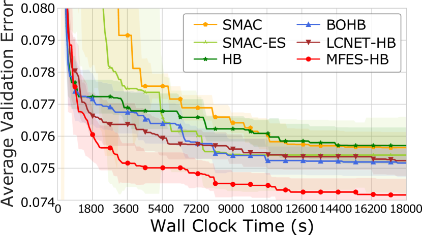
(a) Results on FCNet

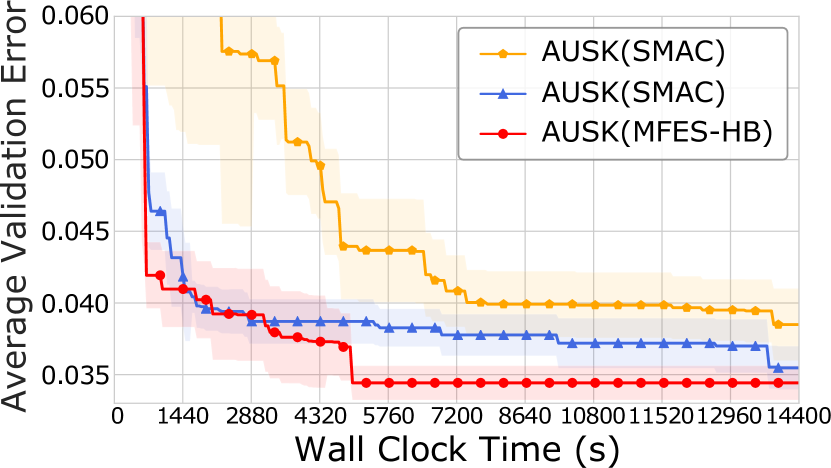
(b) AutoML

Figure 4: Results for optimizing FCNet on MNIST (sequential) and AutoML on Letter (parallel).

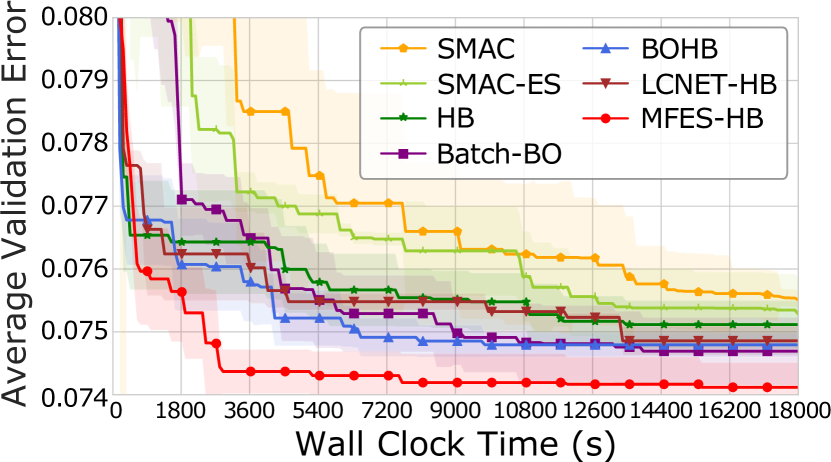
(a) FCNet

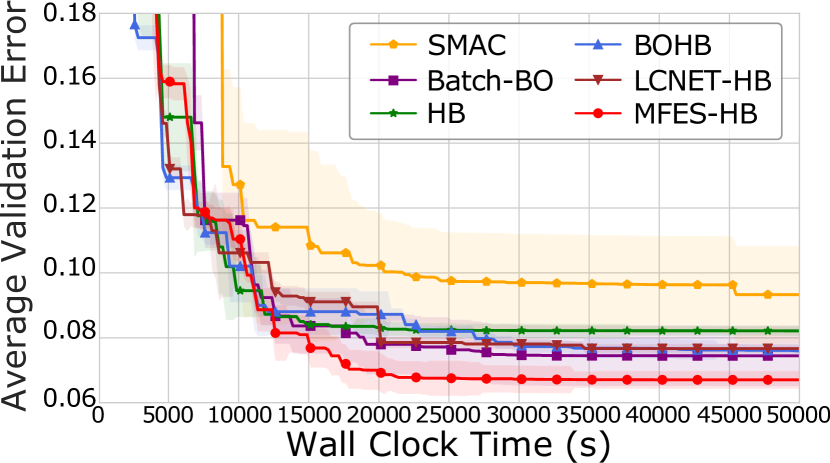
(b) ResNet

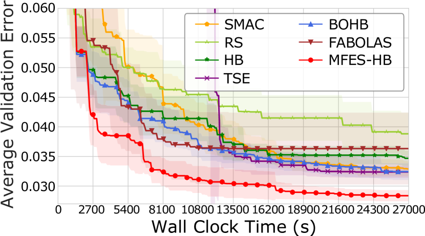
(c) XGBoost

Figure 5: Results for optimizing FCNet on MNIST, ResNet on CIFAR-10, and XGBoost on Covtype.

Experiment Settings

Baselines. We compared MFES-HB with the following eight baselines: (1) HB: the original Hyperband (Li et al. 2018), (2) BOHB (Falkner, Klein, and Hutter 2018): a model-based Hyperband that uses TPE-based surrogate fitted on the high-fidelity measurements to sample configurations, (3) LCNET-HB (Klein et al. 2017a): also a model-based Hyperband, it utilizes the LCNet that predicts the learning curve of configurations to sample configurations in HB, (4) SMAC (Hutter, Hoos, and Leyton-Brown 2011): a widely-used BO method with high-fidelity evaluations, (5) SMAC-ES (Domhan, Springenberg, and Hutter 2015): a variant of SMAC with the learning curve extrapolation-based early stopping, (6) Batch-BO (González et al. 2016): a parallel BO method that conducts a batch of high-fidelity evaluations concurrently. (7) FABOLAS (Klein et al. 2017b) and (8) TSE (Hu et al. 2019): the multi-fidelity optimization methods that utilize the cheap fidelities of $f$ on subsets of the training data. Besides the two compared MF methods (FABOLAS and TSE), we also considered the following 3 methods: MF-MES (Takeno et al. 2020), taKG (Wu et al. 2019a) and MTBO (Swersky, Snoek, and Adams 2013).

HPO Tasks. Table 2 describes 4 real-world AutoML HPO tasks in our experiments. For example, in FCNet, we optimized $10$ hyperparameters on MNIST; the resource type is the number of iterations; one unit of resource corresponds to 0.5 epoch, and the total HPO budget $B_{hpo}$ for each baseline is $5$ hours. In addition, to investigate the practicability and the performance of MFES-HB in AutoML systems, we also implemented MFES-HB in Auto-Sklearn (AUSK) (Feurer et al. 2015), and compared it with the built-in HPO method — SMAC in AUSK, on 10 public datasets. More details about the configuration space $\mathcal{X}$ and datasets (12 in total) can be found in Appendix A.2 and A.3 respectively.

Dataset Split, Metric and Parameter Setting. In each experiment, we randomly divided 20% of the training dataset as the validation set, tracked the wall clock time (including optimization overhead and evaluation cost), and stored the lowest validation error after each evaluation. All methods are repeated 10 times with different random seeds, and the mean($\pm$std) validation errors across runs are plotted. Moreover, the best models found by the baselines are applied to the test dataset, and test errors are reported. All methods are discussed based on two metrics: (1) the time taken for reaching the same validation error, (2) the test performance. As recommended by HB and BOHB, $\eta$ is set to $3$ for the HB-based methods, and $\rho=0.2$. In MFES-HB, we implemented the MFES based on the probabilistic random forest from the SMAC package; the parameter $\theta$ used in weight discrimination operator is set to $3$. Figure 3 (c) depicts the sensitivity analysis about $\theta$. The same parallel mechanism in BOHB is adopted in the parallel experiments. More details about the experiment settings, hardware, the parameter settings of baselines, and their implementations (including source code) are available in Appendix A.4, A.5, and A.6.

Empirical Analysis

Figures 3 and  4(a) illustrate the results on FCNet, where we investigated (1) the feasibility of the low-fidelity measurements and (2) the effectiveness of MFES. Figures 5 and  4(b) show the results on four HPO tasks, where we studied the efficiency of MFES-HB. Table 3 lists the test results. Below, we will verify four insights based on these results.

Using low-fidelity quality measurements brings benefits. Figure 3 (a) shows the results of (1) the different versions of MFES that utilize the multi-fidelity measurements and (2) BOHB that uses the high-fidelity measurements only, on FCNet. MFES with single best surrogate means that it uses the base surrogate with the smallest ranking loss defined in Eq.3 to sample configurations in HB. MFES with equal weight means that, for each surrogate $M_{i}$, $w_{i}=\frac{1}{K}$. MFES refers to the proposed ensemble surrogate with a ranking loss based weight calculation method. We can observe that using low-fidelity measurements can bring benefits to achieve a faster convergence in HPO.

MFES can exploit the multi-fidelity measurements effectively. From Figure 3(a), we can find that two variants (MFES with the single best surrogate and MFES with equal weight) cannot beat the proposed MFSE method using gPoE. As shown in Figure 3(c), gPOE is more reasonable and effective in combining the base surrogates than the linear combination under the independent assumption (LC-idp curve). Based on the above results, the proposed MFSE, which combines base surrogates using gPOE with the ranking loss based weight calculation technique, is an effective surrogate to utilize the multi-fidelity measurements. To further investigate the weight update process, the values of $w_{i}$s across iterations are illustrated in Figure 3(b). The surrogates trained on the lowest-fidelity measurements and the scarce high-fidelity measurements have relatively smaller weights; the surrogates with medium-fidelity measurements own larger weights. Figure 3(c) depicts the parameter sensitivity check of $\theta$. Finally, Figure 4(a) shows the HPO results of all methods on FCNet, and MFES-HB obtains a (more than) $5\times$ speedup over the baselines.

Method	FCNet	ResNet	XGB
SMAC	7.63	9.10	3.52
SMAC (ES)	7.49	8.37	-
Batch BO	7.47	7.98	3.00
HB	7.55	8.40	3.56
LCNET-HB	7.49	8.21	-
BOHB	7.48	8.10	3.16
FABOLAS	-	-	3.40
TSE	-	-	3.12
MFES-HB	7.38	7.49	2.65

(a) Test results of baselines

Dataset	AUSK	AUSK(new)
MNIST	3.39	2.15
Letter	3.85	3.44
Higgs	26.84	26.79
Electricity	6.18	6.21
Kropt	19.84	13.08
Mv	0.03	0.01
Poker	12.91	4.30
Fried	6.60	6.62
A9a	17.23	17.09
2dplanes	6.59	6.41

(b) Results on 10 AutoML datasets

Table 3: Mean test errors (%) of compared baselines. In Table(a), since SMAC (ES) & LCNET-HB depend on training iteration and FABOLAS & TSE only work on sample size, ‘-’ means the invalid cases. In Table(b), AUSK(new) represents Auto-Sklearn using MFES-HB as its HPO optimizer.

Method	Error	Speedups
HB	7.53	1.0x
BOHB	7.48	3.05x
MTBO	7.50	1.07x
MF-MES	7.45	5.7x
taKG	7.46	4.8x
MFES-HB	7.41	10.1x

(a) Results on FCNet

Method	Error	Speedups
HB	3.48	1.0x
BOHB	3.26	1.8x
MTBO	3.46	F
MF-MES	3.11	3.1x
taKG	3.16	2.9x
MFES-HB	2.97	4.5x

(b) Results on XGBoost

Table 4: Speedup result over Hyperband (HB) on two benchmarks: FCNet and XGBoost. ‘F’ means the method fails to reach the result of HB.

MFES-HB can accelerate HPO tasks. Figures 5 and  4(b) depict the empirical results on four HPO tasks, where the tasks on FCNet and ResNet are conducted in parallel settings. MFES-HB spends less time than the compared methods to obtain a sub-optimal performance. Concretely, MFES-HB achieves the validation error of 7.5% on FCNet within 0.75 hours, 7.3% on ResNet within 4.3 hours, and 3.5% on XGBoost within 2.25 hours. To reach the same results, it takes other methods about 5 hours on FCNet, 13.9 hours on ResNet, and 7.5 hours on XGBoost. MFES-HB achieves the $3.2$ to $6.7\times$ speedups in finding a similar configuration. Particularly, MFES-HB achieves $4.05$ to $10.1\times$ speedups over Hyperband, and $3.3$ to $8.9\times$ speedups over the state-of-the-art BOHB. Moreover, Table 3 (a) shows that the configuration found by MFES-HB gets the best test performance. In addition, when comparing MF-MES, taKG, and MTBO, the final results and speedups over HB in achieving the same final error of HB are reported in Table 4. MFES-HB outperforms these methods, and we see that MFES-HB, which combines the benefits of HB and MFBO, works well. Therefore, this demonstrates that MFES-HB can conduct HPO efficiently and effectively.

The advantages of MFES-HB. MFES-HB can easily handle HPO problems with $6$ to $110$ hyperparameters (scalability). Particularly, the AutoML task on 10 datasets involves a very high-dimensional space: 110 hyperparameters in total. In addition, MFES-HB supports (1) complex hyperparameter space by using the BO component from SMAC (generality), and (2) HPO with different resource types (flexibility); while most multi-fidelity optimization approaches only support one type of resource, and cannot be extended to the other types easily. Finally, on 10 datasets, we compared the performance of MFES-HB with the built-in HPO algorithm (SMAC) in Auto-Sklearn (AUSK). Figure 4(b) shows the results on dataset Letter, and Table 3 (b) demonstrates its practicability and effectiveness in AutoML system.

Conclusion

In this paper, we introduced MFES-HB, an efficient Hyperband method that utilizes multi-fidelity quality measurements to accelerate HPO tasks. The multi-fidelity ensemble surrogate is proposed to integrate quality measurements with multiple fidelities effectively. We evaluated MFES-HB on a wide range of AutoML HPO tasks, and demonstrated its superiority over the competitive approaches.

References

- Baker et al. (2017) Baker, B.; Gupta, O.; Raskar, R.; and Naik, N. 2017. Practical neural network performance prediction for early stopping. arXiv preprint arXiv:1705.10823 2(3): 6.
- Bardenet et al. (2013) Bardenet, R.; Brendel, M.; Kégl, B.; and Sebag, M. 2013. Collaborative hyperparameter tuning. In International Conference on Machine Learning, 199–207.
- Bergstra et al. (2011) Bergstra, J. S.; Bardenet, R.; Bengio, Y.; and Kégl, B. 2011. Algorithms for hyper-parameter optimization. In Advances in neural information processing systems, 2546–2554.
- Bertrand et al. (2017) Bertrand, H.; Ardon, R.; Perrot, M.; and Bloch, I. 2017. Hyperparameter optimization of deep neural networks: Combining hyperband with Bayesian model selection. In Conférence sur l’Apprentissage Automatique.
- Cao and Fleet (2014) Cao, Y.; and Fleet, D. J. 2014. Generalized product of experts for automatic and principled fusion of Gaussian process predictions. arXiv preprint arXiv:1410.7827 .
- Dai et al. (2019) Dai, Z.; Yu, H.; Low, B. K. H.; and Jaillet, P. 2019. Bayesian Optimization Meets Bayesian Optimal Stopping 1496–1506.
- Domhan, Springenberg, and Hutter (2015) Domhan, T.; Springenberg, J. T.; and Hutter, F. 2015. Speeding Up Automatic Hyperparameter Optimization of Deep Neural Networks by Extrapolation of Learning Curves. In IJCAI, volume 15, 3460–8.
- Eggensperger et al. (2013) Eggensperger, K.; Feurer, M.; Hutter, F.; Bergstra, J.; Snoek, J.; Hoos, H.; and Leyton-Brown, K. 2013. Towards an empirical foundation for assessing bayesian optimization of hyperparameters. In NIPS workshop on Bayesian Optimization in Theory and Practice, volume 10, 3.
- Falkner, Klein, and Hutter (2018) Falkner, S.; Klein, A.; and Hutter, F. 2018. BOHB: Robust and Efficient Hyperparameter Optimization at Scale. In Proceedings of the 35th International Conference on Machine Learning, 1436–1445.
- Feurer et al. (2015) Feurer, M.; Klein, A.; Eggensperger, K.; Springenberg, J.; Blum, M.; and Hutter, F. 2015. Efficient and robust automated machine learning. In Advances in neural information processing systems, 2962–2970.
- Feurer, Letham, and Bakshy (2018) Feurer, M.; Letham, B.; and Bakshy, E. 2018. Scalable meta-learning for bayesian optimization using ranking-weighted gaussian process ensembles. In AutoML Workshop at ICML.
- Golovin et al. (2017) Golovin, D.; Solnik, B.; Moitra, S.; Kochanski, G.; Karro, J.; and Sculley, D. 2017. Google vizier: A service for black-box optimization. In Proceedings of the 23rd ACM SIGKDD International Conference on Knowledge Discovery and Data Mining, 1487–1495. ACM.
- González et al. (2016) González, J.; Dai, Z.; Hennig, P.; and Lawrence, N. 2016. Batch bayesian optimization via local penalization. In Artificial Intelligence and Statistics, 648–657.
- Goodfellow, Bengio, and Courville (2016) Goodfellow, I.; Bengio, Y.; and Courville, A. 2016. Deep learning. MIT press.
- He et al. (2017) He, X.; Liao, L.; Zhang, H.; Nie, L.; Hu, X.; and Chua, T.-S. 2017. Neural collaborative filtering. In Proceedings of the 26th international conference on world wide web, 173–182.
- Hinton (1999) Hinton, G. E. 1999. Products of experts .
- Hu et al. (2019) Hu, Y.-Q.; Yu, Y.; Tu, W.-W.; Yang, Q.; Chen, Y.; and Dai, W. 2019. Multi-Fidelity Automatic Hyper-Parameter Tuning via Transfer Series Expansion. AAAI .
- Hutter, Hoos, and Leyton-Brown (2011) Hutter, F.; Hoos, H. H.; and Leyton-Brown, K. 2011. Sequential model-based optimization for general algorithm configuration. In International Conference on Learning and Intelligent Optimization, 507–523. Springer.
- Hutter, Kotthoff, and Vanschoren (2018) Hutter, F.; Kotthoff, L.; and Vanschoren, J., eds. 2018. Automated Machine Learning: Methods, Systems, Challenges. Springer. In press, available at http://automl.org/book.
- Jamieson and Talwalkar (2016) Jamieson, K.; and Talwalkar, A. 2016. Non-stochastic best arm identification and hyperparameter optimization. In Artificial Intelligence and Statistics, 240–248.
- Jiang et al. (2017) Jiang, J.; Jiang, J.; Cui, B.; and Zhang, C. 2017. TencentBoost: a gradient boosting tree system with parameter server. In 2017 IEEE 33rd ICDE, 281–284. IEEE.
- Jones, Schonlau, and Welch (1998) Jones, D. R.; Schonlau, M.; and Welch, W. J. 1998. Efficient global optimization of expensive black-box functions. Journal of Global optimization 13(4): 455–492.
- Kandasamy et al. (2017) Kandasamy, K.; Dasarathy, G.; Schneider, J.; and Poczos, B. 2017. Multi-fidelity bayesian optimisation with continuous approximations. arXiv preprint arXiv:1703.06240 .
- Klein et al. (2017a) Klein, A.; Falkner, S.; Bartels, S.; Hennig, P.; and Hutter, F. 2017a. Fast Bayesian Optimization of Machine Learning Hyperparameters on Large Datasets. In Proceedings of the 20th International Conference on Artificial Intelligence and Statistics, 528–536.
- Klein et al. (2017b) Klein, A.; Falkner, S.; Springenberg, J. T.; and Hutter, F. 2017b. Learning curve prediction with Bayesian neural networks. Proceedings of the International Conference on Learning Representations .
- Li et al. (2018) Li, L.; Jamieson, K.; DeSalvo, G.; Rostamizadeh, A.; and Talwalkar, A. 2018. Hyperband: A novel bandit-based approach to hyperparameter optimization. Proceedings of the International Conference on Learning Representations 1–48.
- Li et al. (2020) Li, Y.; Jiang, J.; Gao, J.; Shao, Y.; Zhang, C.; and Cui, B. 2020. Efficient Automatic CASH via Rising Bandits. In AAAI, 4763–4771.
- Ma et al. (2019) Ma, J.; Wen, J.; Zhong, M.; Chen, W.; and Li, X. 2019. MMM: Multi-source Multi-net Micro-video Recommendation with Clustered Hidden Item Representation Learning. Data Science and Engineering 4(3): 240–253.
- Poloczek, Wang, and Frazier (2017) Poloczek, M.; Wang, J.; and Frazier, P. 2017. Multi-information source optimization. In Advances in Neural Information Processing Systems, 4288–4298.
- Schilling et al. (2015) Schilling, N.; Wistuba, M.; Drumond, L.; and Schmidt-Thieme, L. 2015. Hyperparameter optimization with factorized multilayer perceptrons. In Joint European Conference on Machine Learning and Knowledge Discovery in Databases, 87–103. Springer.
- Schilling, Wistuba, and Schmidt-Thieme (2016) Schilling, N.; Wistuba, M.; and Schmidt-Thieme, L. 2016. Scalable hyperparameter optimization with products of gaussian process experts. In Joint European conference on machine learning and knowledge discovery in databases, 33–48. Springer.
- Sen, Kandasamy, and Shakkottai (2018) Sen, R.; Kandasamy, K.; and Shakkottai, S. 2018. Noisy Blackbox Optimization with Multi-Fidelity Queries: A Tree Search Approach. arXiv: Machine Learning .
- Snoek, Larochelle, and Adams (2012) Snoek, J.; Larochelle, H.; and Adams, R. P. 2012. Practical bayesian optimization of machine learning algorithms. In Advances in neural information processing systems.
- Swersky, Snoek, and Adams (2013) Swersky, K.; Snoek, J.; and Adams, R. P. 2013. Multi-task bayesian optimization. In Advances in neural information processing systems, 2004–2012.
- Swersky, Snoek, and Adams (2014) Swersky, K.; Snoek, J.; and Adams, R. P. 2014. Freeze-thaw Bayesian optimization. arXiv preprint arXiv:1406.3896 .
- Takeno et al. (2020) Takeno, S.; Fukuoka, H.; Tsukada, Y.; Koyama, T.; Shiga, M.; Takeuchi, I.; and Karasuyama, M. 2020. Multi-fidelity Bayesian Optimization with Max-value Entropy Search and its parallelization.
- Wang, Xu, and Wang (2018) Wang, J.; Xu, J.; and Wang, X. 2018. Combination of Hyperband and Bayesian Optimization for Hyperparameter Optimization in Deep Learning .
- Wang et al. (2013) Wang, Z.; Zoghi, M.; Hutter, F.; Matheson, D.; and De Freitas, N. 2013. Bayesian optimization in high dimensions via random embeddings. In Twenty-Third International Joint Conference on Artificial Intelligence.
- Wistuba, Schilling, and Schmidt-Thieme (2016) Wistuba, M.; Schilling, N.; and Schmidt-Thieme, L. 2016. Two-stage transfer surrogate model for automatic hyperparameter optimization. In Joint European conference on machine learning and knowledge discovery in databases, 199–214. Springer.
- Wu et al. (2019a) Wu, J.; Toscano-Palmerin, S.; Frazier, P. I.; and Wilson, A. G. 2019a. Practical multi-fidelity Bayesian optimization for hyperparameter tuning.
- Wu et al. (2019b) Wu, J.; Toscanopalmerin, S.; Frazier, P. I.; and Wilson, A. G. 2019b. Practical multi-fidelity Bayesian optimization for hyperparameter tuning 284.
- Wu et al. (2020) Wu, S.; Zhang, Y.; Gao, C.; Bian, K.; and Cui, B. 2020. GARG: Anonymous Recommendation of Point-of-Interest in Mobile Networks by Graph Convolution Network. Data Science and Engineering ISSN 23641541. doi:10.1007/s41019-020-00135-z.
- Yao et al. (2018) Yao, Q.; Wang, M.; Escalante, H. J.; Guyon, I.; Hu, Y.; Li, Y.; Tu, W.; Yang, Q.; and Yu, Y. 2018. Taking Human out of Learning Applications: A Survey on Automated Machine Learning. CoRR .
- Yogatama and Mann (2014) Yogatama, D.; and Mann, G. 2014. Efficient transfer learning method for automatic hyperparameter tuning. In Artificial Intelligence and Statistics, 1077–1085.
- Zhang et al. (2020) Zhang, W.; Jiang, J.; Shao, Y.; and Cui, B. 2020. Snapshot boosting: a fast ensemble framework for deep neural networks. Sci. China Inf. Sci. 63(1): 112102. doi:10.1007/s11432-018-9944-x. URL https://doi.org/10.1007/s11432-018-9944-x.
- Zöller and Huber (2019) Zöller, M.; and Huber, M. F. 2019. Survey on Automated Machine Learning. CoRR abs/1904.12054.