Persistent Laplacians: properties, algorithms and implications

Abstract

We present a thorough study of the theoretical properties and devise efficient algorithms for the persistent Laplacian, an extension of the standard combinatorial Laplacian to the setting of pairs (or, in more generality, sequences) of simplicial complexes $K\hookrightarrow L$, which was independently introduced by Lieutier et al. and by Wang et al. In particular, in analogy with the non-persistent case, we first prove that the nullity of the $q$-th persistent Laplacian $\Delta_{q}^{K,L}$ equals the $q$-th persistent Betti number of the inclusion $(K\hookrightarrow L)$. We then present an initial algorithm for finding a matrix representation of $\Delta_{q}^{K,L}$, which itself helps interpret the persistent Laplacian. We exhibit a novel relationship between the persistent Laplacian and the notion of Schur complement of a matrix which has several important implications. In the graph case, it both uncovers a link with the notion of effective resistance and leads to a persistent version of the Cheeger inequality. This relationship also yields an additional, very simple algorithm for finding (a matrix representation of) the $q$-th persistent Laplacian which in turn leads to a novel and fundamentally different algorithm for computing the $q$-th persistent Betti number for a pair $(K,L)$ which can be significantly more efficient than standard algorithms. Finally, we study persistent Laplacians for simplicial filtrations and present novel stability results for their eigenvalues. Our work brings methods from spectral graph theory, circuit theory, and persistent homology together with a topological view of the combinatorial Laplacian on simplicial complexes.

1 Introduction

The combinatorial graph Laplacian, as an operator on functions defined on the vertex set of a graph, is a fundamental object in the analysis of and optimization on graphs. Its spectral properties are widely used in graph optimization problems (e.g, spectral clustering [9, 34, 43, 52]) and in the efficient solution of systems of equations, cf. [30, 37, 49, 51]. The graph Laplacian is also connected to network circuit theory via the notion of effective resistance [2, 11, 38, 48].

There is also an algebraic topology view of the graph Laplacian which arises through considering boundary operators and specific inner products defined on simplicial (co)chain groups [9]. This permits extending the graph Laplacian to a more general operator, the $q$-th combinatorial Laplacian $\Delta_{q}^{K}$ on the $q$-th (co)chain groups of a given simplicial complex $K$ (see e.g., [14, 13, 18, 25]), so that the standard graph Laplacian simply corresponds to the 0-th case. These ideas connect to the topology of the input simplicial complex via the so called combinatorial Hodge Theorem [14], which states that the nullity of the $q$-th combinatorial Laplacian is equal to the rank of the $q$-th cohomology group of $K$ with real coefficients, i.e. the $q$-th Betti number of $K$. See also [25, 36] for thorough expositions.

The combinatorial Laplacian (and variants) have received a great deal of attention in recent years; see e.g. [18, 19, 20, 41]. For example, [29] aims to extend the related concept, effective resistance from network circuit theory, to this “high dimensional” situation, whereas [22, 21] consider a spectral theory of cellular sheaves with applications to sparsification and synchronization problems.

Adopting the algebraic topology view of the $q$-th combinatorial Laplacian, [35] and [53] independently introduced the so-called $q$-th persistent Laplacian $\Delta_{q}^{K,L}$, which is an extension of the combinatorial Laplacian mentioned above to a pair of simplicial complexes $K\hookrightarrow L$ connected by an inclusion. To the best of our knowledge, [35] and [53] are the first works which establishes a link between persistent homology [15, 57], one of the most important developments in the field of applied and computational topology in the past two decades, with the Laplacian, a common and fundamental object with a vast literature, both in the theoretical and applied domains. See also [10, 45] for other work in computational topology which leverages ideas connected to the (standard) combinatorial Laplacian.

It is thus natural and also highly desirable to achieve better understanding, as well as algorithmic developments, for this persistent Laplacian, all of which will help broaden its potential applications. The present paper aims to close this gap.

Contributions

In this paper, we carry out a thorough study of the properties of and develop algorithms for the persistent Laplacian. Our work brings together ideas and methods from several communities, including spectral graph theory, circuit theory, topological treatments of high-dimensional combinatorial Laplacians, together with a persistent homology perspective (both at the theoretical and algorithmic levels). For instance, we relate the computation of persistent homology with notions from network theory such as the Kron reduction (and also Schur complements) which have novel algorithmic implications; see below.

This is an overview of our results:

• In Section 2, we present several results about the properties of the $q$-th persistent Laplacian $\Delta_{q}^{K,L}$, including Theorem 2.7, which establishes that the nullity of $\Delta_{q}^{K,L}$ equals the $q$-th persistent Betti number from $K$ to $L$: a result analogous to the one that holds in the non-persistent case.

• In Section 3, we give a first algorithm (Algorithm 1) to compute a matrix representation of $\Delta_{q}^{K,L}$, which relies on matrix reduction ideas which are standard when computing persistent homology.

• In Section 4, we establish our main observation Theorem 4.6, a relationship between the persistent Laplacian and the concept of Schur complement of a matrix. This observation has several immediate and important implications:

  1. We establish a second, very simple algorithm (Algorithm 2) which computes the matrix representation of the persistent Laplacian $\Delta_{q}^{K,L}$ (for any $q$) efficiently, purely based on a linear algebraic formulation (Theorem 4.6).

  2. This observation leads to a new algorithm to compute the $q$-th persistent Betti number for a pair of spaces in a fundamentally different manner from extant algorithms in the computational topology literature. This new algorithm is, under mild conditions (e.g. as those commonly satisfied by Vietoris-Rips complexes) significantly more efficient than existing algorithms. We believe that this new algorithm for computing persistent Betti numbers is of independent interest.

  3. In the graph case (i.e. when $K$ and $L$ are graphs and $q=0$), this provides a direct connection with notions from network circuit theory such as the Kron reduction [11], a connection which reveals that the matrix representation of the persistent Laplacian permits recovering the effective resistance of pairs of vertices in $K$ w.r.t the larger graph $L$ (cf. Proposition 4.9 and Theorem 4.10). The connection with network circuit theory leads to our definition of a “persistent” Cheeger constant as well as to a novel persistent Cheeger-like inequality for a pair of graphs $K\hookrightarrow L$ (cf. Section 4.4).

• Finally, in Section 5, we consider $q$-th persistent Laplacians for filtrations of simplicial complexes (connected by inclusion morphisms). We first describe an efficient algorithm to iteratively compute the persistent Laplacian for all all pairs of complexes in a filtration. We then discuss certain spectral stability results for the persistent Laplacian for filtrations of simplicial complexes.

Some technical details are relegated to the appendix.

2 The persistent Laplacian for simplicial pairs $K\hookrightarrow L$

In this section, after introducing some basic notions/definitions in Section 2.1, we formulate the persistent Laplacian for simplicial pairs in Section 2.2 and present some basic properties of persistent Laplacians in Section 2.3.

2.1 Basics

Simplicial complexes

An (abstract) simplicial complex $K$ over a finite ordered set $V$ is a collection of finite subsets of $V$ such that for any $\sigma\in K$, if $\tau\subseteq\sigma$, then $\tau\in K$. Denote by $\mathbb{N}$ the set of non-negative integers. For each $q\in\mathbb{N}$, an element $\sigma\in K$ is called a $q$-simplex if $|\sigma|=q+1$, where we use $|A|$ to denote the cardinality of a set $A$. A $0$-simplex, usually denoted by $v$, is also called a vertex. Denote by $S_{q}^{K}$ the set of $q$-simplices of $K$. Note that $S_{0}^{K}\subseteq V$. The dimension of $K$, denoted by $\dim(K)$, is the largest $q$ such that $S_{q}^{K}\neq\emptyset$. A $1$-dim simplicial complex is also called a graph and we often use $K=(V^{K},E^{K})$ to represent a graph, where $V^{K}\coloneqq S_{0}^{K}$ denotes the vertex set and $E^{K}\coloneqq S_{1}^{K}$ denotes the edge set.

An oriented simplex, denoted by $[\sigma]$, is a simplex $\sigma\in K$ with an ordering on its vertices. For simplicity of our presentation, we always assume that the ordering is inherited from the ordering of $V$. Let $\bar{S}_{q}^{K}\coloneqq\left\{[\sigma]:\,\sigma\in S_{q}^{K}\right\}$. The $q$-th chain group $C_{q}^{K}\coloneqq C_{q}(K,\mathbb{R})$ of $K$ is the vector space over $\mathbb{R}$ with basis $\bar{S}_{q}^{K}$. Let $n_{q}^{K}\coloneqq\dim C_{q}^{K}=\left|S_{q}^{K}\right|$. We define the boundary operator $\partial_{q}^{K}:C_{q}^{K}\rightarrow C_{q-1}^{K}$ by

$$\partial_{q}^{K}([v_{0},\ldots,v_{q}])\coloneqq\sum_{i=0}^{q}(-1)^{i}[v_{0},\ldots,\hat{v}_{i},\ldots,v_{q}]$$ (1)

for each $\sigma=[v_{0},\ldots,v_{q}]\in\bar{S}_{q}^{K}$, where $\hat{v}_{i}$ denotes the omission of the $i$-th vertex. The $q$-th homology group of $K$ is $H_{q}(K)=\frac{\ker\left(\partial_{q}^{K}\right)}{\mathrm{im}\left(\partial_{q+1}^{K}\right)}$ and $\beta_{q}^{K}\coloneqq\mathrm{rank}\left(H_{q}(K)\right)$ is its $q$-th Betti number.

A weight function on a simplicial complex $K$ is any positive function $w^{K}:K\rightarrow(0,\infty)$. Throughout the paper, each simplicial complex $K$ is (implicitly) endowed with a weight function $w^{K}$. We call $K$ unweighted if $w^{K}\equiv 1$.

Combinatorial Laplacian

Let $K$ be a simplicial complex with a weight function $w^{K}$. Given any $q\in\mathbb{N}$, let $w_{q}^{K}\coloneqq w^{K}|_{S_{q}^{K}}$ and define the inner product $\langle\cdot,\cdot\rangle_{w_{q}^{K}}$ on $C_{q}^{K}$ as follows:

$$\langle[\sigma],[\sigma^{\prime}]\rangle_{w_{q}^{K}}\coloneqq\delta_{\sigma\sigma^{\prime}}\cdot\left(w_{q}^{K}(\sigma)\right)^{-1},\,\,\forall\sigma,\sigma^{\prime}\in S_{q}^{K}.$$ (2)

Remark 2.1.

Consider the dual space of $C_{q}^{K}$: the cochain space $C^{q}(K)\coloneqq\mathrm{Hom}\left(C_{q}(K),\mathbb{R}\right)$. Then, $\langle\cdot,\cdot\rangle_{w_{q}^{K}}$ on $C_{q}(K)$ induces an inner product $\llangle\cdot,\cdot\rrangle_{{w}_{q}^{K}}$ on $C^{q}(K)$ such that

$$\llangle f,g\rrangle_{{w}_{q}^{K}}=\sum_{\sigma\in S_{q}^{K}}w_{q}^{K}(\sigma)f([\sigma])g([\sigma]),\,\,\,\forall f,g\in C^{q}(K).$$

This inner product $\llangle\cdot,\cdot\rrangle_{{w}_{q}^{K}}$ on $C^{q}(K)$ coincides with the one defined in [25], which explains the reciprocal in the definition Equation 2 of the inner product $\langle\cdot,\cdot\rangle_{w_{q}^{K}}$ on $C_{q}(K)$.

We denote by $\left(\partial_{q}^{K}\right)^{*}:C_{q-1}^{K}\rightarrow C_{q}^{K}$ the adjoint of $\partial_{q}^{K}$ under these inner products. Then, we define the $q$-th (combinatorial) Laplacian $\Delta_{q}^{K}:C_{q}^{K}\rightarrow C_{q}^{K}$ as follows:

$$\Delta_{q}^{K}\coloneqq\underbrace{\partial_{q+1}^{K}\circ\left(\partial_{q+1}^{K}\right)^{\ast}}_{\Delta^{K}_{q,\mathrm{up}}}+\underbrace{\left(\partial_{q}^{K}\right)^{\ast}\circ\partial_{q}^{K}}_{\Delta_{q,\mathrm{down}}^{K}},$$ (3)

where for convenience we have also defined the corresponding “up” and “down” Laplacians. By convention we let $\partial_{0}^{K}\coloneqq 0$ and thus $\Delta_{0}^{K}=\partial_{1}^{K}\circ\left(\partial_{1}^{K}\right)^{\ast}.$ When $K$ is a graph and $w_{0}^{K}\equiv 1$, $\Delta_{0}^{K}$ reduces to the graph Laplacian of the weighted graph $(K,w_{1}^{K})$ [9].

Theorem 2.2 ([14]).

For each $q\in\mathbb{N}$, $\beta_{q}^{K}=\mathrm{nullity}\left(\Delta_{q}^{K}\right)$.

Simplicial pairs and simplicial filtrations

A simplicial pair, denoted $K\hookrightarrow L$, consists of any pair $K$ and $L$ of simplicial complexes over the same finite ordered set $V$ such that $K\subseteq L$, i.e., $S_{q}^{K}\subseteq S_{q}^{L}$ for all $q\in\mathbb{N}$, and $w^{K}=w^{L}|_{K}$. A simplicial filtration $\mathbf{K}=\{K_{t}\}_{t\in T}$ is a set of simplicial complexes over the same finite ordered set $V$ indexed by a subset $T\subseteq\mathbb{R}$ such that for all $s\leq t\in T$, $K_{s}\hookrightarrow K_{t}$ is a simplicial pair. For an integer $q\geq 0$ and for any $s\leq t\in T$, via functoriality of Homology [23] one obtains a map $f^{s,t}_{q}:H_{q}(K_{s})\rightarrow H_{q}(K_{t})$ and the $q$-th persistent homology groups are defined as the images of these maps. The $q$-th persistent Betti numbers $\beta_{q}^{s,t}$ of $\mathbf{K}$ are in turn defined as the ranks of these groups. Of course when one is just presented with a simplicial pair $K\hookrightarrow L$, for each $q$ one also obtains the analogously defined $q$-th persistent Betti number $\beta^{K,L}_{q}$.

2.2 Definition of the persistent Laplacian

Suppose that we have a simplicial pair $K\hookrightarrow L$ and that $q\in\mathbb{N}$. Consider the subspace

$$C_{q}^{L,K}\coloneqq\left\{c\in C^{L}_{q}\,:\,\partial_{q}^{L}(c)\in C_{q-1}^{K}\right\}\subseteq C_{q}^{L}$$

consisting of those $q$-chains in $C_{q}^{L}$ such that their images under the boundary operator $\partial_{q}^{L}$ is in the subspace $C_{q-1}^{K}$ of $C_{q-1}^{L}$. Let $n_{q}^{L,K}\coloneqq\dim\left(C_{q}^{L,K}\right)$.

Now, for each $q$ let $\partial_{q}^{L,K}$ denote the restriction of $\partial_{q}^{L}$ to $C_{q}^{L,K}$ so that we obtain the “diagonal” operators $\partial_{q}^{L,K}:C_{q}^{L,K}\rightarrow C_{q-1}^{K}$. As we mentioned earlier, for each $q$ both $C^{K}_{q}$ and $C^{L}_{q}$ are endowed with inner products $\langle\cdot,\cdot\rangle_{w_{q}^{K}}$ and $\langle\cdot,\cdot\rangle_{w_{q}^{L}}$ so that we can consider the adjoints of $\partial_{q+1}^{L,K}$ and $\partial_{q}^{L}$. See the diagram below for the construction where the blue arrows signal the important part of the diagram:

One can then define the $q$-th persistent Laplacian [53] $\Delta_{q}^{K,L}:C_{q}^{K}\rightarrow C_{q}^{K}$ by:

$$\Delta_{q}^{K,L}\coloneqq\underbrace{\partial_{q+1}^{L,K}\circ\left(\partial_{q+1}^{L,K}\right)^{\ast}}_{\Delta^{K,L}_{q,\mathrm{up}}}+{\left(\partial_{q}^{K}\right)^{\ast}\circ\partial_{q}^{K}},$$ (4)

where we have also defined the $q$-th up persistent Laplacian $\Delta^{K,L}_{q,\mathrm{up}}$ with the same domain/codomain as $\Delta_{q}^{K,L}$. When $q=0$, since $\partial_{0}^{K}=0$, $\Delta_{0}^{K,L}=\partial_{1}^{K,L}\circ\left(\partial_{1}^{K,L}\right)^{\ast}=\Delta^{K,L}_{0,\mathrm{up}}.$

Example 2.3 (Trivial cases).

1. When $C_{q+1}^{L,K}=\{0\}$, $\partial_{q+1}^{L,K}=0$ and thus $\Delta^{K,L}_{q,\mathrm{up}}=0$.

2. When $K=L$, then obviously $\Delta_{q}^{K,L}=\Delta_{q}^{L}$, the usual Laplacian on $L$.

3. If $S_{q}^{K}=S_{q}^{L}$, then $\Delta_{q,\mathrm{up}}^{K,L}=\Delta_{q,\mathrm{up}}^{L}$. In particular, if $S_{0}^{K}=S_{0}^{L}$, then $\Delta_{0}^{K,L}=\Delta_{0}^{L}$. If furthermore $S_{q-1}^{K}=S_{q-1}^{L}$, then $\Delta_{q,\mathrm{down}}^{K}=\Delta_{q,\mathrm{down}}^{L}$ and thus $\Delta_{q}^{K,L}=\Delta_{q}^{L}$.

Obviously, $\Delta_{q}^{K,L}$ is a self-adjoint, non-negative and compact operator on $C_{q}^{K}$ and thus has non-negative real eigenvalues. We denote by $0\leq\lambda_{q,1}^{K,L}\leq\lambda_{q,2}^{K,L}\leq\ldots\leq\lambda_{q,n_{q}^{K}}^{K,L}$ the eigenvalues of $\Delta_{q}^{K,L}$ sorted in increasing order, including repetitions.

2.3 Basic properties of the persistent Laplacian

We now show some basic properties of $\Delta_{q}^{K,L}$. All proofs are given in Appendix A.

Lemma 2.4.

Suppose $L$ has $n$ connected components $L_{1},\ldots,L_{n}$. Suppose $K$ only intersects the first $m$ connected components. Let $K_{i}\coloneqq K\cap L_{i}$ for each $i=1,\ldots,m$. Then, $\Delta_{q}^{K,L}$ is the direct sum of persistent Laplacians $\Delta_{q}^{K_{i},L_{i}}$ on $C_{q}^{K_{i}}$ for $i=1,\ldots,m$, i.e., $\Delta_{q}^{K,L}=\bigoplus_{i=1}^{m}\Delta_{q}^{K_{i},L_{i}}.$

Given a graph $K$, the multiplicity of the 0 eigenvalue of $\Delta_{0}^{K}$ coincides with the number of connected components of $K$ [40]. The following result is a persistent version of this.

Theorem 2.5.

The eigenvalues of $\Delta_{0}^{K,L}$ satisfy the following basic properties.

1. $\lambda_{0,1}^{K,L}=0$; and if $L$ is connected, then $\lambda_{0,2}^{K,L}>0$.

2. Let $m$ be the multiplicity of the $0$ eigenvalue of $\Delta_{0}^{K,L}$, then $K$ intersects exactly $m$ connected components of $L$.

We have a complete description of the behavior of the up persistent Laplacian on interior simplices, where a $q$-simplex $\sigma\in S_{q}^{K}$ is called an interior simplex if $\sigma$ only shares cofaces with $q$-simplices in $K$, i.e., $\forall\sigma^{\prime}\in S_{q}^{L},$ if $\sigma\cup\sigma^{\prime}\in S_{q+1}^{L},$ then $\sigma^{\prime}\in S_{q}^{K}.$

Theorem 2.6.

Let $c^{L}\in C_{q}^{L}$ and let $c^{K}$ be the image of $c^{L}$ under the orthogonal projection $C_{q}^{L}\rightarrow C_{q}^{K}$. Then, for any interior simplex $\sigma\in S_{q}^{K}$, we have that

$$\left\langle\Delta_{q,\mathrm{up}}^{L}c^{L},[\sigma]\right\rangle_{w_{q}^{L}}=\left\langle\Delta_{q,\mathrm{up}}^{K,L}c^{K},[\sigma]\right\rangle_{w_{q}^{K}}.$$

The following result showing persistent Laplacians recover persistent Betti numbers was mentioned in passing and without proof in [53] and was also implicitly contained in pages 10 and 11 of [35]. We give a full proof in Appendix A.

Theorem 2.7.

For each integer $q\geq 0$, we have that $\beta_{q}^{K,L}=\mathrm{nullity}\left(\Delta_{q}^{K,L}\right)$.

3 A first algorithm for computing a matrix representation of $\Delta_{q}^{K,L}$

In this section, we first provide a matrix representation $\boldsymbol{\Delta}_{q}^{K,L}$ of $\Delta_{q}^{K,L}$ given the canonical basis $\bar{S}_{q}^{K}$ of $C_{q}^{K}$ and then devise an algorithm for computing $\boldsymbol{\Delta}_{q}^{K,L}$.

Note: For simplicity, given a simplicial pair $K\hookrightarrow L$, for each $q\in\mathbb{N}$ we assume an ordering $\bar{S}_{q}^{L}=\{[\sigma_{i}]\}_{i=1}^{n_{q}^{L}}$ on $\bar{S}_{q}^{L}$ such that $\bar{S}_{q}^{K}=\{[\sigma_{i}]\}_{i=1}^{n_{q}^{K}}$. Unless otherwise specified, matrix representations of operators between chain groups are always from such orderings on canonical bases $\bar{S}_{q}^{K}$ and $\bar{S}_{q}^{L}$ of $C_{q}^{K}$ and $C_{q}^{L}$, respectively.

Theorem 3.1.

Assume that $n_{q+1}^{L,K}\coloneqq\dim\left(C_{q+1}^{L,K}\right)>0$. Choose any basis of $C_{q+1}^{L,K}\subseteq C_{q+1}^{L}$ represented by a column matrix $Z\in\mathbb{R}^{n_{q+1}^{L}\times n_{q+1}^{L,K}}$. Let $B_{q}^{K}$ and $B_{q+1}^{L,K}$ be matrix representations of boundary maps $\partial_{q}^{K}$ and $\partial_{q+1}^{L,K}$, respectively. Let $W_{q}^{K}$ (or $W_{q}^{L}$) denote the diagonal weight matrix representation of $w_{q}^{K}$ (or $w_{q}^{L}$). Then, the matrix representation $\boldsymbol{\Delta}_{q}^{K,L}$ of $\Delta_{q}^{K,L}$ is expressed as follows:

$$\boldsymbol{\Delta}_{q}^{K,L}=\underbrace{B_{q+1}^{L,K}\left(Z^{\mathrm{T}}\left(W_{q+1}^{L}\right)^{-1}Z\right)^{-1}\left(B_{q+1}^{L,K}\right)^{\mathrm{T}}\left(W_{q}^{K}\right)^{-1}}_{\boldsymbol{\Delta}_{q,\mathrm{up}}^{K,L}}+\underbrace{W_{q}^{K}\left(B_{q}^{K}\right)^{\mathrm{T}}\left(W_{q-1}^{K}\right)^{-1}B_{q}^{K}}_{\boldsymbol{\Delta}_{q,\mathrm{down}}^{K}}.$$ (5)

Moreover, $\boldsymbol{\Delta}_{q}^{K,L}$ is invariant under the choice of basis for $C_{q+1}^{L,K}$.

Remark 3.2 (Matrix representations of combinatorial Laplacians).

When $K=L$, Equation 5 reduces to the matrix representation of the combinatorial Laplacian:

$$\boldsymbol{\Delta}_{q}^{K}\coloneqq\underbrace{B_{q+1}^{K}W_{q+1}^{K}\left(B_{q+1}^{K}\right)^{\mathrm{T}}\left(W_{q}^{K}\right)^{-1}}_{\boldsymbol{\Delta}^{K}_{q,\mathrm{up}}}+\underbrace{W_{q}^{K}\left(B_{q}^{K}\right)^{\mathrm{T}}\left(W_{q-1}^{K}\right)^{-1}B_{q}^{K}}_{\boldsymbol{\Delta}_{q,\mathrm{down}}^{K}}.$$

Since $B_{q+1}^{K}W_{q+1}^{K}\left(B_{q+1}^{K}\right)^{\mathrm{T}}\left(W_{q}^{K}\right)^{-1}=\left(W_{q}^{K}\right)^{\frac{1}{2}}\left(\left(W_{q}^{K}\right)^{-\frac{1}{2}}B_{q+1}^{K}W_{q+1}^{K}\left(B_{q+1}^{K}\right)^{\mathrm{T}}\left(W_{q}^{K}\right)^{-\frac{1}{2}}\right)\left(W_{q}^{K}\right)^{-\frac{1}{2}},$ $\boldsymbol{\Delta}_{q,\mathrm{up}}^{K}$ is of the form $W^{-1}PW$ where $P$ is symmetric positive semi-definite and $W$ is a positive diagonal matrix. The same result holds for down Laplacians, up persistent Laplacians, and (persistent) Laplacians. Note that if $w_{q}^{K}\equiv 1$, then $\boldsymbol{\Delta}_{q}^{K}={B_{q+1}^{K}W_{q+1}^{K}\left(B_{q+1}^{K}\right)^{\mathrm{T}}}+{\left(B_{q}^{K}\right)^{\mathrm{T}}\left(W_{q-1}^{K}\right)^{-1}B_{q}^{K}}$ is itself a symmetric positive semi-definite matrix.

To prove the theorem, we need the following result:

Lemma 3.3.

Let $f:(\mathbb{R}^{n},W_{n})\rightarrow(\mathbb{R}^{m},W_{m})$ be a linear map where $W_{n}\in\mathbb{R}^{n\times n}$ and $W_{m}\in\mathbb{R}^{m\times m}$ denote the inner product matrices. Let $F\in\mathbb{R}^{m\times n}$ denote the matrix representation of $f$. Then, the matrix representation $F^{*}$ of the adjoint $f^{*}$ of $f$ is $W_{n}^{-1}F^{\mathrm{T}}W_{m}$.

Proof.

For any $x=(x_{1},\ldots,x_{n})^{\mathrm{T}}\in\mathbb{R}^{n}$ and $y=(y_{1},\ldots,y_{m})^{\mathrm{T}}\in\mathbb{R}^{m}$, we have that

$$\left\langle fx,y\right\rangle_{\mathbb{R}^{m}}=\left(Fx\right)^{\mathrm{T}}W_{m}y=x^{\mathrm{T}}F^{\mathrm{T}}W_{m}y,\text{ and }\,\left\langle x,f^{*}y\right\rangle_{\mathbb{R}^{n}}=x^{\mathrm{T}}W_{n}F^{*}y.$$

Since $\left\langle fx,y\right\rangle_{\mathbb{R}^{m}}=\left\langle x,f^{*}y\right\rangle_{\mathbb{R}^{n}}$ and $x,y$ are arbitrary, we must have that $F^{*}=W_{n}^{-1}F^{\mathrm{T}}W_{m}$. ∎

Proof of Theorem 3.1.

Base on our choice of bases for $C_{q+1}^{L,K}$, $C_{q}^{K}$ and $C_{q-1}^{K}$, the corresponding inner product matrices are $Z^{\mathrm{T}}\left(W_{q+1}^{L}\right)^{-1}Z$, $\left(W_{q}^{K}\right)^{-1}$ and $\left(W_{q-1}^{K}\right)^{-1}$, respectively. By Lemma 3.3, the matrix representation for $(\partial_{q+1}^{L,K})^{\ast}$ is $\left(Z^{\mathrm{T}}\left(W_{q+1}^{L}\right)^{-1}Z\right)^{-1}(B_{q+1}^{L,K})^{\mathrm{T}}\left(W_{q}^{K}\right)^{-1}$ and the matrix representation for $(\partial_{q}^{K})^{\ast}$ is $W_{q}^{K}\left(B_{q}^{K}\right)^{\mathrm{T}}\left(W_{q-1}^{K}\right)^{-1}$. By Equation 4, we have

$$\boldsymbol{\Delta}_{q}^{K,L}=B_{q+1}^{L,K}\left(Z^{\mathrm{T}}\left(W_{q+1}^{L}\right)^{-1}Z\right)^{-1}\left(B_{q+1}^{L,K}\right)^{\mathrm{T}}\left(W_{q}^{K}\right)^{-1}+W_{q}^{K}\left(B_{q}^{K}\right)^{\mathrm{T}}\left(W_{q-1}^{K}\right)^{-1}B_{q}^{K}.$$

Since $\partial_{q+1}^{L,K}\left(\partial_{q+1}^{L,K}\right)^{\ast}$ is a self-operator on $C_{q}^{K}$, its matrix representation $\boldsymbol{\Delta}_{q}^{K,L}$ only depends on the choice of basis of $C_{q}^{K}$ and it is thus independent of the choice of basis of $C_{q+1}^{L,K}$. ∎

An algorithm for computing the matrix representation of $\Delta_{q}^{K,L}$

We use the symbol $[n]$ to denote the set $\{1,\ldots,n\}$ for a positive integer $n$. We first introduce a notation for representing submatrices. Let $M\in\mathbb{R}^{m\times n}$ be a real matrix and let $\emptyset\neq I\subseteq[m]$ and $\emptyset\neq J\subseteq[n]$. We denote by $M(I,J)$ the submatrix of $M$ consisting of those rows and columns indexed by $I$ and $J$, respectively. Moreover, we use $M(:,J)$ (or $M(I,:)$) to denote $M([m],J)$ (or $M(I,[n])$).

By Theorem 3.1, to compute a matrix representation of $\Delta_{q}^{K,L}$, the key is to produce a basis (i.e., $Z$) for $C_{q+1}^{L,K}$. Let $B_{q+1}^{L}\in\mathbb{R}^{n_{q}^{L}\times n_{q+1}^{L}}$ be the matrix representation of the boundary map $\partial_{q+1}^{L}$. We assume that $n_{q}^{K}<n_{q}^{L}$ since the case $n_{q}^{K}=n_{q}^{L}$ is trivial (cf. Example 2.3). Then, the following lemma (proof in Appendix A) suggests a way of constructing $Z$ from $B_{q+1}^{L}$.

Lemma 3.4.

Let $D_{q+1}^{L}\coloneqq B_{q+1}^{L}\left([n_{q}^{L}]\backslash[n_{q}^{K}],:\right)$. Then, there exists a non-singular matrix $Y\in\mathbb{R}^{n_{q+1}^{L}\times n_{q+1}^{L}}$ such that $R_{q+1}^{L}\coloneqq D_{q+1}^{L}Y$ is column reduced. Moreover, let $I\subseteq[n_{q+1}^{L}]$ be the index set of $0$ columns of $R_{q+1}^{L}$. The following hold:

1. If $I=\emptyset$, then $C_{q+1}^{L,K}=\{0\}$;

2. If $I\neq\emptyset$, let $Z\coloneqq Y(:,I)$, then columns of $Z$ constitute a basis of $C_{q+1}^{L,K}$.

Moreover, if $I\neq\emptyset$, then $B_{q+1}^{L,K}\coloneqq\left(B_{q+1}^{L}Y\right)\left([n_{q}^{K}],I\right)$ is the matrix representation of $\partial_{q+1}^{L,K}$.

We can apply a column reduction process (e.g., Gaussian elimination) to $D_{q+1}^{L}$ to obtain $Y\in\mathbb{R}^{n_{q+1}^{L}\times n_{q+1}^{L}}$ and $R_{q+1}^{L}\coloneqq D_{q+1}^{L}Y$ requested in Lemma 3.4. See Algorithm 1 for a pseudocode for computing $\boldsymbol{\Delta}_{q}^{K,L}$ based on Lemma 3.4.

Algorithm 1 Persistent Laplacian: matrix representation

1:  Data: $B_{q}^{K},B_{q+1}^{L},W_{q-1}^{K},W_{q}^{K}$ and $W_{q+1}^{L}$

2:  Result: $\boldsymbol{\Delta}_{q}^{K,L}$

3:  compute $\boldsymbol{\Delta}_{q,\mathrm{down}}^{K}$ from $B_{q}^{K},W_{q-1}^{K}$ and $W_{q}^{K}$

4:  if $n_{q}^{K}==n_{q}^{L}$ then

5:     compute $\boldsymbol{\Delta}_{q,\mathrm{up}}^{L}$ from $B_{q+1}^{L},W_{q}^{K}$ and $W_{q+1}^{L}$;   

6:     return  $\boldsymbol{\Delta}_{q,\mathrm{up}}^{L}+\boldsymbol{\Delta}_{q,\mathrm{down}}^{K}$

7:  end if

8:  $D_{q+1}^{L}=B_{q+1}^{L}\left([n_{q}^{L}]\backslash[n_{q}^{K}],:\right)$

9:  $(R_{q+1}^{L},Y)=\mathrm{ColumnReduction}(D_{q+1}^{L})$

10:  $I\leftarrow$ index set corresponding to the all-zero columns of $R_{q+1}^{L}$

11:  if $I==\emptyset$ then

12:     return  $\boldsymbol{\Delta}_{q,\mathrm{down}}^{K}$

13:  end if

14:  $Z=Y(:,I)$

15:  $B_{q+1}^{L,K}=\left(B_{q+1}^{L}Y\right)\left([n_{q}^{K}],I\right)$

16:  

17:  return  $B_{q+1}^{L,K}\left(Z^{\mathrm{T}}\left(W_{q+1}^{L}\right)^{-1}Z\right)^{-1}\left(B_{q+1}^{L,K}\right)^{\mathrm{T}}\left(W_{q}^{K}\right)^{-1}+\boldsymbol{\Delta}_{q,\mathrm{down}}^{K}$

Complexity analysis

The computation of $\boldsymbol{\Delta}_{q,\mathrm{down}}^{K}$ takes time $O\left(\left(n_{q}^{K}\right)^{2}\right)$ (See Appendix B for details). The size of $D_{q+1}^{L}$ is $\left(n_{q}^{L}-n_{q}^{K}\right)\times n_{q+1}^{L}$; thus the column reduction process takes time $O\left((n_{q}^{L}-n_{q}^{K})\left(n_{q+1}^{L}\right)^{2}\right)$. Computing the product $B_{q+1}^{L}Y$ takes time $O\left(n_{q}^{L}\left(n_{q+1}^{L}\right)^{2}\right)$. The size of $Z$ is $n_{q+1}^{L}\times|I|$, where $|I|\leq n_{q+1}^{L}$. Then, computing $\left(Z^{\mathrm{T}}\left(W_{q+1}^{L}\right)^{-1}Z\right)^{-1}$ takes time $O\left(\left(n_{q+1}^{L}\right)^{3}\right)$. The product $B_{q+1}^{L,K}\left(Z^{\mathrm{T}}\left(W_{q+1}^{L}\right)^{-1}Z\right)^{-1}\left(B_{q+1}^{L,K}\right)^{\mathrm{T}}\left(W_{q}^{K}\right)^{-1}$ can be computed in time $O\left(n_{q}^{K}\left(n_{q+1}^{L}\right)^{2}\right)$. Hence Algorithm 1 takes $O\left(n_{q}^{L}\left(n_{q+1}^{L}\right)^{2}+\left(n_{q+1}^{L}\right)^{3}+\left(n_{q}^{K}\right)^{2}\right)$ total time. One can also improve this time complexity by using fast matrix-multiplication to both perform reduction and compute multiplication/inverse. We omit the details.

4 Schur complement, persistent Laplacian and implications

Let $M\in\mathbb{R}^{n\times n}$ be a block matrix $M=\begin{pmatrix}A&B\\ C&D\end{pmatrix}$ where $D\in\mathbb{R}^{d\times d}$ is a square matrix. Then, the (generalized) Schur complement of $D$ in $M$ [5], denoted by $M/D$, is $M/D\coloneqq A-BD^{\dagger}C$, where $D^{\dagger}$ is the Moore-Penrose generalized inverse of $D$. Note that having $D$ to be the bottom right submatrix is only for notational simplicity. Schur complement is defined for any principal submatrix. More precisely, let $\emptyset\neq I\subsetneq[n]$ be a proper subset. Then, the (generalized) Schur complement of $M(I,I)$ in $M$ is defined as

$$M/M(I,I)\coloneqq M([n]\backslash I,[n]\backslash I)-M([n]\backslash I,I)M(I,I)^{\dagger}M(I,[n]\backslash I).$$ (6)

Now we introduce some useful properties of the Schur complement.

Definition 4.1 (Proper submatrices).

Let $M=\begin{pmatrix}A&B\\ C&D\end{pmatrix}$ be a square block matrix where both $A$ and $D$ are square matrices. The submatrix $D$ is proper in $M$ if $\ker(D)\subseteq\ker(B)$ and $\ker\left(D^{\mathrm{T}}\right)\subseteq\ker\left(C^{\mathrm{T}}\right)$.

Lemma 4.2 (Positive semi-definite matrices).

Let $P$ be a positive semi-definite block matrix $P=\begin{pmatrix}A&B\\ C&D\end{pmatrix}$ such that $A$ and $D$ are square matrices. Let $W$ be a positive diagonal matrix and we write $W$ as a block matrix $W=\begin{pmatrix}W_{1}&0\\ 0&W_{2}\end{pmatrix}$ such that $W_{1}$ and $W_{2}$ have the same sizes as $A$ and $D$, respectively. Consider $M\coloneqq W^{-1}PW=\begin{pmatrix}W_{1}^{-1}AW_{1}&W_{1}^{-1}BW_{2}\\ W_{2}^{-1}CW_{1}&W_{2}^{-1}DW_{2}\end{pmatrix}$. Then, $W_{2}^{-1}DW_{2}$ is proper in $M$ and $M/(W_{2}^{-1}DW_{2})=W_{1}^{-1}(P/D)W_{1}.$

Lemma 4.3 ([5, Theorem 1]).

Let $M$ be a square block matrix $M=\begin{pmatrix}A&B\\ C&D\end{pmatrix}$ such that $A$ and $D$ are square matrices. Then, $\mathrm{rank}(M)\geq\mathrm{rank}(D)+\mathrm{rank}(M/D).$

Lemma 4.4 (Quotient Formula [5, Theorem 4]).

Let $M,D$ and $H$ be square matrices with the following block structures: $M=\begin{pmatrix}A&B\\ C&D\end{pmatrix}\text{ and }D=\begin{pmatrix}E&F\\ G&H\end{pmatrix}.$ If $D$ is proper in $M$ and $H$ is proper in $D$, then $D/H$ is proper in $M/H$ and $M/D=(M/H)/(D/H).$

Lemma 4.5 (Eigenvalue interlacing property).

Let $M=W^{-1}PW$ be as in Lemma 4.2. Suppose that the size of $M$ is $n\times n$ and the size of $D$ is $d\times d$. Then,

$$\lambda_{k}(M)\leq\lambda_{k}(M/(W_{2}^{-1}DW_{2}))\leq\lambda_{k}(W_{1}^{-1}AW_{1}),\quad\forall 1\leq k\leq n-d,$$ (7)

where $\lambda_{k}(A)$ denotes the $k$-th smallest eigenvalue of $A$ (counted with multiplicity).

See Appendix A for proofs of Lemma 4.2 and Lemma 4.5.

4.1 Up-persistent Laplacian as a Schur complement

For a simplicial pair $K\hookrightarrow L$, recall from Section 3 that for each $q\in\mathbb{N}$ we assume an ordering $\bar{S}_{q}^{L}=\{[\sigma_{i}]\}_{i=1}^{n_{q}^{L}}$ on $\bar{S}_{q}^{L}$ such that $\bar{S}_{q}^{K}=\{[\sigma_{i}]\}_{i=1}^{n_{q}^{K}}$. Given such orderings on canonical bases of $C_{q}^{K}$ and $C_{q}^{L}$, the matrix representation $\boldsymbol{\Delta}_{q,\mathrm{up}}^{K,L}$ of $\Delta_{q,\mathrm{up}}^{K,L}:C_{q}^{K}\rightarrow C_{q}^{K}$ is related to the matrix representation $\boldsymbol{\Delta}_{q,\mathrm{up}}^{L}$ of $\Delta_{q,\mathrm{up}}^{L}:C_{q}^{L}\rightarrow C_{q}^{L}$ via the Schur complement as follows:

Theorem 4.6 (Up-persistent Laplacian as Schur complement).

Let $K\hookrightarrow L$ be a simplicial pair. Assume that $n_{q}^{K}<n_{q}^{L}$ and let $I_{K}^{L}\coloneqq[n_{q}^{L}]\backslash[n_{q}^{K}]$. Then,

$$\boldsymbol{\Delta}_{q,\mathrm{up}}^{K,L}=\boldsymbol{\Delta}_{q,\mathrm{up}}^{L}/\boldsymbol{\Delta}_{q,\mathrm{up}}^{L}\left(I_{K}^{L},I_{K}^{L}\right).$$ (8)

To prove the above theorem, we first need the following lemma (whose proof is given in Appendix A) which relates Schur complements with a certain matrix operation.

Lemma 4.7.

Let $B\in\mathbb{R}^{n\times m}$ be a block matrix $B=\begin{pmatrix}B_{1}\\ B_{2}\end{pmatrix}$, where $B_{1}\in\mathbb{R}^{d\times m}$ for some $1\leq d<n$. Let $W_{1}\in\mathbb{R}^{d\times d}$ and $W_{2}\in\mathbb{R}^{(n-d)\times(n-d)}$ be non-singular diagonal matrices and let $W=\begin{pmatrix}W_{1}&0\\ 0&W_{2}\end{pmatrix}$. Let $M\coloneqq BB^{\mathrm{T}}W$, which is a block matrix

$$M=\begin{pmatrix}M_{11}&M_{12}\\ M_{21}&M_{22}\end{pmatrix}=\begin{pmatrix}B_{1}B_{1}^{\mathrm{T}}W_{1}&B_{1}B_{2}^{\mathrm{T}}W_{2}\\ B_{2}B_{1}^{\mathrm{T}}W_{1}&B_{2}B_{2}^{\mathrm{T}}W_{2}\end{pmatrix}.$$

If $B_{2}$ has full column rank, then $M/M_{22}=0$. Otherwise, for any non-singular block matrix $Y=\begin{pmatrix}Y_{1}&Y_{2}\end{pmatrix}\in\mathbb{R}^{m\times m}$, if $B_{2}Y_{1}=0$ and $B_{2}Y_{2}$ has full column rank, then $M/M_{22}=B_{1}Y_{1}\left(Y_{1}^{\mathrm{T}}Y_{1}\right)^{-1}(B_{1}Y_{1})^{\mathrm{T}}W_{1}.$

Proof of Theorem 4.6.

Let $B\coloneqq B_{q+1}^{L}\left(W_{q+1}^{L}\right)^{\frac{1}{2}}$, $W\coloneqq W_{q}^{L}$ and $W_{1}\coloneqq W([n_{q}^{K}],[n_{q}^{K}])=W_{q}^{K}$. Set $B_{1}\coloneqq B\left([n_{q}^{K}],:\right)$ and $B_{2}\coloneqq B\left([n_{q}^{L}]\backslash[n_{q}^{K}],:\right)$. Then, $B=\begin{pmatrix}B_{1}\\ B_{2}\end{pmatrix}$. Note that $B_{2}=D_{q+1}^{L}\left(W_{q+1}^{L}\right)^{\frac{1}{2}}$ using notations in Lemma 3.4. By Lemma 3.4, there exists a non-singular matrix $\hat{Y}\in\mathbb{R}^{n_{q+1}^{L}\times n_{q+1}^{L}}$ such that $R_{q+1}^{L}\coloneqq D_{q+1}^{L}\hat{Y}$ is column reduced. Let $Y\coloneqq\left(W_{q+1}^{L}\right)^{-\frac{1}{2}}\hat{Y}$, which is still non-singular. Then,

$$R_{q+1}^{L}=D_{q+1}^{L}\hat{Y}=D_{q+1}^{L}\left(W_{q+1}^{L}\right)^{\frac{1}{2}}\left(W_{q+1}^{L}\right)^{-\frac{1}{2}}\hat{Y}=B_{2}Y.$$

Let $I\subseteq[n_{q+1}^{L}]$ be the index set of $0$ columns of $R_{q+1}^{L}$. If $I=\emptyset$, then by Lemma 3.4 we have that $C_{q+1}^{L,K}=\{0\}$ and thus $\boldsymbol{\Delta}_{q,\mathrm{up}}^{K,L}=0$. On the other hand, $I=\emptyset$ implies that $B_{2}$ has full column rank. Let $M\coloneqq BB^{\mathrm{T}}W$. Then, we have that

$$M=B_{q+1}^{L}W_{q+1}^{L}\left(B_{q+1}^{L}\right)^{\mathrm{T}}W_{q}^{L}=\boldsymbol{\Delta}_{q,\mathrm{up}}^{L}$$

and thus $M_{22}=\boldsymbol{\Delta}_{q,\mathrm{up}}^{L}\left(I_{K}^{L},I_{K}^{L}\right)$. Then by Lemma 4.7, we have that

$$\boldsymbol{\Delta}_{q,\mathrm{up}}^{L}/\boldsymbol{\Delta}_{q,\mathrm{up}}^{L}\left(I_{K}^{L},I_{K}^{L}\right)=M/M_{22}=0=\boldsymbol{\Delta}_{q,\mathrm{up}}^{K,L}.$$

Now, we assume that $I\neq\emptyset$. Without loss of generality, we assume that $I=[n_{q+1}^{L,K}]\subseteq[n_{q+1}^{L}]$ (otherwise we multiply $Y$ by a permutation matrix). Let $Y_{1}\coloneqq Y\left(:,I\right)=\left(W_{q+1}^{L}\right)^{-\frac{1}{2}}Z$ where $Z$ is a column matrix representing a basis of $C_{q+1}^{L,K}$ (cf. Lemma 3.4). Let $Y_{2}\coloneqq Y\left(:,[n_{q+1}^{L}]\backslash I\right)$. Then, $Y=\begin{pmatrix}Y_{1}&Y_{2}\end{pmatrix}$ is a block matrix such that $B_{2}Y_{1}=R_{q+1}^{L}(:,I)=0$ and that $B_{2}Y_{2}=R_{q+1}^{L}\left(:,[n_{q+1}^{L}]\backslash I\right)$ has full column rank. Then, by Lemma 4.7, we have that

$$\boldsymbol{\Delta}_{q,\mathrm{up}}^{L}/\boldsymbol{\Delta}_{q,\mathrm{up}}^{L}\left(I_{K}^{L},I_{K}^{L}\right)=M/M_{22}=B_{1}Y_{1}\left(Y_{1}^{\mathrm{T}}Y_{1}\right)^{-1}(B_{1}Y_{1})^{\mathrm{T}}W_{1}$$

$$= B_{1}\left(W_{q+1}^{L}\right)^{-\frac{1}{2}}Z\left(\left(\left(W_{q+1}^{L}\right)^{-\frac{1}{2}}Z\right)^{\mathrm{T}}\left(W_{q+1}^{L}\right)^{-\frac{1}{2}}Z\right)^{-1}\left(B_{1}\left(W_{q+1}^{L}\right)^{-\frac{1}{2}}Z\right)^{\mathrm{T}}W_{q}^{K}$$

$$= B_{1}\left(W_{q+1}^{L}\right)^{-\frac{1}{2}}Z\left(Z^{\mathrm{T}}\left(W_{q+1}^{L}\right)^{-1}Z\right)^{-1}\left(B_{1}\left(W_{q+1}^{L}\right)^{-\frac{1}{2}}Z\right)^{\mathrm{T}}W_{q}^{K}.$$

Note also that $B_{q+1}^{L,K}=B_{q+1}^{L}([n_{q}^{K}],:)Z=B_{1}\left(W_{q+1}^{L}\right)^{-\frac{1}{2}}Z$. Then, by Lemma 3.4 we have that

$$\boldsymbol{\Delta}_{q,\mathrm{up}}^{K,L}=B_{q+1}^{L,K}\left(Z^{\mathrm{T}}\left(W_{q+1}^{L}\right)^{-1}Z\right)^{-1}\left(B_{q+1}^{L,K}\right)^{\mathrm{T}}W_{q}^{K}=\boldsymbol{\Delta}_{q,\mathrm{up}}^{L}/\boldsymbol{\Delta}_{q,\mathrm{up}}^{L}\left(I_{K}^{L},I_{K}^{L}\right).$$

This finishes the proof of Theorem 4.6. ∎

4.2 Fast computation of the matrix representation of $\Delta_{q}^{K,L}$

For a simplicial pair $K\hookrightarrow L$, by Theorem 4.6, we now simply compute $\boldsymbol{\Delta}_{q,\mathrm{up}}^{K,L}$ via Equation 8 using only Schur complement computations, which then give us $\boldsymbol{\Delta}_{q}^{K,L}=\boldsymbol{\Delta}_{q,\mathrm{up}}^{K,L}+\boldsymbol{\Delta}_{q,\mathrm{down}}^{K}$. A pseudocode for this simple algorithm is given in Algorithm 2.

Algorithm 2 Persistent Laplacian: matrix representation via Schur complement

1:  Data: $B_{q}^{K},B_{q+1}^{L},W_{q-1}^{K},W_{q}^{K},W_{q}^{L}$ and $W_{q+1}^{L}$

2:  Result: $\boldsymbol{\Delta}_{q}^{K,L}$

3:  Compute $\boldsymbol{\Delta}_{q,\mathrm{down}}^{K}$ from $B_{q}^{K},W_{q-1}^{K}$ and $W_{q}^{K}$

4:  Compute $\boldsymbol{\Delta}_{q,\mathrm{up}}^{L}$ from $B_{q+1}^{L},W_{q}^{L}$ and $W_{q+1}^{L}$

5:  if $n_{q}^{K}==n_{q}^{L}$ then

6:     return  $\boldsymbol{\Delta}_{q,\mathrm{up}}^{L}+\boldsymbol{\Delta}_{q,\mathrm{down}}^{K}$

7:  end if

8:  $\boldsymbol{\Delta}_{q,\mathrm{up}}^{K,L}=\boldsymbol{\Delta}_{q,\mathrm{up}}^{L}/\boldsymbol{\Delta}_{q,\mathrm{up}}^{L}\left(I_{K}^{L},I_{K}^{L}\right)$

9:  

10:  return  $\boldsymbol{\Delta}_{q,\mathrm{up}}^{K,L}+\boldsymbol{\Delta}_{q,\mathrm{down}}^{K}$

Time complexity

Computing $\boldsymbol{\Delta}_{q,\mathrm{up}}^{L}$ takes time $O\left(n_{q+1}^{L}\right)$ and computing $\boldsymbol{\Delta}_{q,\mathrm{down}}^{K}$ takes $O\left(\left(n_{q}^{K}\right)^{2}\right)$ (see Appendix B for details). The Schur complement $\boldsymbol{\Delta}_{q,\mathrm{up}}^{L}/\boldsymbol{\Delta}_{q,\mathrm{up}}^{L}\left(I_{K}^{L},I_{K}^{L}\right)$ takes time

$$O\left(\left(n_{q}^{K}\right)^{2}+\left(n_{q}^{L}-n_{q}^{K}\right)^{3}+n_{q}^{K}\left(n_{q}^{L}-n_{q}^{K}\right)^{2}\right)=O\left(\left(n_{q}^{L}\right)^{3}\right)$$

to compute. Hence the total time complexity of computing $\boldsymbol{\Delta}_{q}^{K,L}$ via Equation 8 is $O\left(\left(n_{q}^{L}\right)^{3}+n_{q+1}^{L}\right)$, which is more efficient than the complexity of Algorithm 1, $O\left(n_{q}^{L}\left(n_{q+1}^{L}\right)^{2}+\left(n_{q+1}^{L}\right)^{3}+\left(n_{q}^{K}\right)^{2}\right)$, when $n_{q}^{L}=O(n_{q+1}^{L})$. By using fast matrix multiplication algorithm (which takes $O(r^{\omega})$, $\omega<2.373$, to multiply two $r\times r$ matrices), this time complexity can be improved to $O\left(\left(n_{q}^{L}\right)^{\omega}+n_{q+1}^{L}\right)$.

Computation of persistent Betti numbers

By Theorem 2.7, we can compute the persistent Betti number $\beta_{q}^{K,L}$ in the following manner: we first compute $\boldsymbol{\Delta}_{q}^{K,L}$ and then compute $\beta_{q}^{K,L}=\mathrm{nullity}\left(\boldsymbol{\Delta}_{q}^{K,L}\right)$. Since calculating the nullity of an $n_{q}^{K}\times n_{q}^{K}$ square matrix can be done in time $O\left(\left(n_{q}^{K}\right)^{\omega}\right)=O\left(\left(n_{q}^{L}\right)^{\omega}\right)$, we obtain a method for computing the persistent Betti number in time $O\left(\left(n_{q}^{L}\right)^{\omega}+n_{q+1}^{L}\right)$ (which is $O\left(\left(n_{q}^{L}\right)^{\omega}\right)$ if $n_{q}^{L}=O\left(n_{q+1}^{L}\right)$). Currently, the existing approach in the literature to compute the persistent Betti numbers is through computing the persistent homology of the pair $K\hookrightarrow L$ using boundary matrices $B_{q+1}^{L}$ and $B_{q}^{K}$, which can be done in $O\left(\left(n_{q}^{L}\right)^{2}n_{q+1}^{L}+\left(n_{q-1}^{K}\right)^{2}n_{q}^{K}\right)$ time or in $O\left(\left(n_{q}^{L}\right)^{\omega-1}n_{q+1}^{L}+\left(n_{q-1}^{K}\right)^{\omega-1}n_{q}^{K}\right)$ (if we assume that $n_{q}^{L}=O(n_{q+1}^{L})$ and $n_{q-1}^{K}=O\left(n_{q}^{K}\right)$) using earliest basis (via fast matrix multiplication) approach [3]. Our new algebraic formulation of persistent Laplacian (via Schur complement) thus also leads to a faster algorithm to compute the persistent Betti number for a pair of spaces for the setting when $n_{q}^{L}=O(n_{q+1}^{L})$. Note that the condition $n_{q}^{L}=O(n_{q+1}^{L})$ holds in many practical scenarios, especially for the popular Rips or Čech complexes and their variants. Given that this new algorithm is fundamentally different from existing ones (using only simple Schur complement computations), we believe that this is of independent interest.

Remark 4.8.

A MATLAB implementation of Algorithm 2 for unweighted simplicial pairs is given in [42]. A recent preprint [54] by some of the authors of [53] describes an alternative software implementation of the persistent Laplacian which is available at [55].

4.3 Relationship with the notion of effective resistance

Let $K=(V^{K},E^{K},w^{K})$ be a connected weighted graph. Unless otherwise specified, for any weighted graph considered in this section, we assume that $w^{K}$ satisfies that $w^{K}_{0}=w^{K}|_{S_{0}^{K}}\equiv 1$, i.e., the vertices of the graph are unweighted. For any two vertices $v,w\in V^{K}$, we let $\partial_{[v,w]}\coloneqq-[v]+[w]\in C_{0}^{K}$. Let $D_{[v,w]}^{K}\coloneqq\chi_{w}-\chi_{v}\in\mathbb{R}^{n_{0}^{K}}$ denote the vector representation of $\partial_{[v,w]}$ in $C_{0}^{K}$, where $\chi_{v}\in\mathbb{R}^{n_{0}^{K}}$ is the indicator vector of $v\in V^{K}$. We consider that each edge $e\in E^{K}$ has an electrical conductance $w^{K}(e)$. Then, the effective resistance $\mathfrak{R}_{v,w}^{K}$ between $v$ and $w$ is defined by

$$\mathfrak{R}_{v,w}^{K}\coloneqq\left(D_{[v,w]}^{K}\right)^{\mathrm{T}}\left(\boldsymbol{\Delta}_{0}^{K}\right)^{\dagger}D_{[v,w]}^{K}.$$ (9)

Given a graph pair $K\hookrightarrow L$, by Theorem 4.6 the persistent Laplacian $\boldsymbol{\Delta}_{0}^{K,L}$ turns out to be the graph Laplacian of a new weighted graph.

Proposition 4.9 ([11, Lemma 2.1]).

Suppose that $K\hookrightarrow L$ is a graph pair. Assume that $L$ is connected and $w^{L}_{0}\equiv 1$. Then, $\boldsymbol{\Delta}_{0}^{K,L}=\boldsymbol{\Delta}_{0,\mathrm{up}}^{K,L}$ is the graph Laplacian $\boldsymbol{\Delta}_{0}^{\tilde{K}}$ of a connected weighted graph $\tilde{K}=\left(V^{\tilde{K}},E^{\tilde{K}},w^{\tilde{K}}\right)$ such that $V^{\tilde{K}}=V^{K}$.

$\tilde{K}$ is known as the Kron reduction of $L$ and $\boldsymbol{\Delta}_{0}^{\tilde{K}}$ is called the Kron-reduced matrix. The Kron reduction [31] has been used in network circuit theory, and it preserves effective resistance (cf. [11, Theorem 3.8]). This in turn implies that the persistent Laplacian $\boldsymbol{\Delta}_{0}^{K,L}$ is able to recover the effective resistance $\mathfrak{R}_{v,w}^{L}$ w.r.t. the larger graph $L$ for all pairs of vertices $v,w\in K$. The result below follows from Theorem 4.6 and [11, Theorem 3.8].

Theorem 4.10.

Let $K\hookrightarrow L$ be a graph pair where $L$ is connected. Let $\tilde{K}=(V^{K},E^{\tilde{K}},w^{\tilde{K}})$ denote the weighted graph such that $\boldsymbol{\Delta}_{0}^{\tilde{K}}=\boldsymbol{\Delta}_{0}^{K,L}$. Then, $\tilde{K}$ is connected and for two distinct vertices $v,w\in V^{K}$, we have that $\mathfrak{R}_{v,w}^{L}=\mathfrak{R}_{v,w}^{\tilde{K}}.$

Remark 4.11 (Higher dimensional generalization).

The effective resistance has been generalized to the case of simplicial complexes in [29]. In Appendix F, we show a higher-dimensional extension of Theorem 4.10, i.e., that higher dimensional effective resistances are preserved by the up persistent Laplacian, the proof of which deals with the subtleties of the Moore-Penrose generalized inverse directly without resorting to a limiting argument as in the proof of [11, Theorem 3.8]. In addition, we provide an example illustrating the impossibility of a higher dimensional generalization of the Kron reduction in the current simplicial setting.

The following result controls the change of degrees after applying the Kron reduction.

Proposition 4.12.

Let $\tilde{K}$ be the graph described in Proposition 4.9. Then, for any $v\in V^{K}=V^{\tilde{K}}$, we have that $\mathrm{deg}^{\tilde{K}}(v)\leq\mathrm{deg}^{L}(v)$, where $\mathrm{deg}^{G}(v)\coloneqq\sum_{w\in G}w^{G}(\{v,w\})$ is the weighted degree of a vertex in a graph $G$.

Proof.

We first observe that $\mathrm{deg}^{G}(v)\coloneqq\sum_{w\in G}w^{G}(\{v,w\})=\left(\chi_{v}^{G}\right)^{\mathrm{T}}\boldsymbol{\Delta}_{0}^{G}\chi_{v}$. Therefore,

$$\mathrm{deg}^{\tilde{K}}(v) =\left(\chi_{v}^{K}\right)^{\mathrm{T}}\boldsymbol{\Delta}_{0}^{\tilde{K}}\chi_{v}^{\tilde{K}}=\left(\chi_{v}^{\tilde{K}}\right)^{\mathrm{T}}\boldsymbol{\Delta}_{0}^{K,L}\chi_{v}^{\tilde{K}}=\left(\chi_{v}^{\tilde{K}}\right)^{\mathrm{T}}\boldsymbol{\Delta}_{0}^{L}/\boldsymbol{\Delta}_{0}^{L}(I_{K}^{L},I_{K}^{L})\chi_{v}^{\tilde{K}}$$

$$=\left(\chi_{v}^{\tilde{K}}\right)^{\mathrm{T}}\boldsymbol{\Delta}_{0}^{L}\left([n_{0}^{K}],[n_{0}^{K}]\right)\chi_{v}^{\tilde{K}}-\left(\chi_{v}^{\tilde{K}}\right)^{\mathrm{T}}\boldsymbol{\Delta}_{0}^{L}\left([n_{0}^{K}],I_{K}^{L}\right)\left(\boldsymbol{\Delta}_{0}^{L}\left(I_{K}^{L},I_{K}^{L}\right)\right)^{\dagger}\boldsymbol{\Delta}_{0}^{L}\left(I_{K}^{L},[n_{0}^{K}]\right)\chi_{v}^{\tilde{K}}$$

$$\leq\left(\chi_{v}^{\tilde{K}}\right)^{\mathrm{T}}\boldsymbol{\Delta}_{0}^{L}\left([n_{0}^{K}],[n_{0}^{K}]\right)\chi_{v}^{\tilde{K}}=\left(\chi_{v}^{L}\right)^{\mathrm{T}}\boldsymbol{\Delta}_{0}^{L}\chi_{v}^{L}=\mathrm{deg}^{L}(v)$$

∎

In the case when $K$ consists of only two points in $L$, we have the following explicit relation between the persistent Laplacian and the effective resistance.

Corollary 4.13.

Let $L$ be a connected graph and let $K$ be a two-vertex subgraph with vertex set $V^{K}=\{v,w\}$. Then, $\boldsymbol{\Delta}_{0}^{K,L}=\begin{pmatrix}\frac{1}{\mathfrak{R}_{v,w}^{L}}&-\frac{1}{\mathfrak{R}_{v,w}^{L}}\\ -\frac{1}{\mathfrak{R}_{v,w}^{L}}&\frac{1}{\mathfrak{R}_{v,w}^{L}}\end{pmatrix}$.

Proof of Corollary 4.13.

By Theorem 4.10 (or by [11, Lemma 3.10]), it is easy to show that $\left(\boldsymbol{\Delta}_{0}^{K,L}\right)^{\dagger}=\begin{pmatrix}\frac{\mathfrak{R}_{v,w}^{L}}{4}&-\frac{\mathfrak{R}_{v,w}^{L}}{4}\\ -\frac{\mathfrak{R}_{v,w}^{L}}{4}&\frac{\mathfrak{R}_{v,w}^{L}}{4}\end{pmatrix}.$ Therefore, $\boldsymbol{\Delta}_{0}^{K,L}=\begin{pmatrix}\frac{1}{\mathfrak{R}_{v,w}^{L}}&-\frac{1}{\mathfrak{R}_{v,w}^{L}}\\ -\frac{1}{\mathfrak{R}_{v,w}^{L}}&\frac{1}{\mathfrak{R}_{v,w}^{L}}\end{pmatrix}.$ ∎

4.3.1 Effective resistance between disjoint sets

The effective resistance between two vertices has been generalized to the case of two disjoint sets of vertices in [38, Exercise 2.13] via an energy minimization process. In [47], a formula invoking the graph Laplacian was used to define the effective resistance between disjoint sets. The two definitions are equivalent (see Section D.1 for a proof) and in this section we adopt the definition from [47].

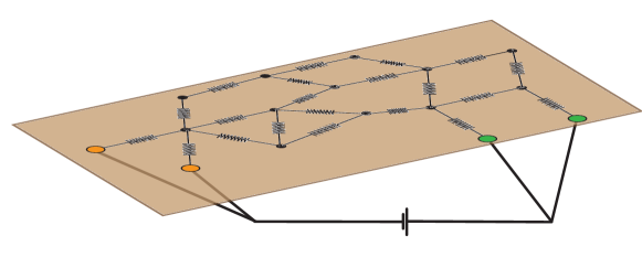
Figure 1: The effective resistance between two sets of vertices from the circuit theory perspective. One set is represented by the orange nodes, the other onbe by the green nodes. See Section D.1 for more details.

Let $K$ be a connected weighted graph. For any non-empty disjoint subsets $A,B\subseteq V^{K}$, let $V^{J}\coloneqq A\cup B$ and let $J$ be the induced subgraph with vertex set $V^{J}$. Then, following [47], the effective resistance $\mathfrak{R}^{K}_{A,B}$ between $A$ and $B$ is defined as follows

$$\mathfrak{R}^{K}_{A,B}\coloneqq\left(\left(\chi_{A}^{J}\right)^{\mathrm{T}}\cdot\boldsymbol{\Delta}_{0}^{K}/\boldsymbol{\Delta}_{0}^{K}\left(V^{J},V^{J}\right)\cdot\chi_{A}^{J}\right)^{-1},$$ (10)

where $\boldsymbol{\Delta}_{0}^{K}\left(V^{J},V^{J}\right)$ denotes the submatrix of $\boldsymbol{\Delta}_{0}^{K}$ with rows and columns indexed by $V^{J}$ and $\chi_{A}^{J}\in\mathbb{R}^{n_{0}^{J}}$ denotes the indicator vector of $A\subseteq V^{J}$. By Theorem 4.6, we have that $\mathfrak{R}^{K}_{A,B}=\left(\left(\chi_{A}^{J}\right)^{\mathrm{T}}\cdot\boldsymbol{\Delta}_{0}^{J,K}\cdot\chi_{A}^{J}\right)^{-1}$. In particular, when $A\cup B=V^{J}=V^{K}$, $\mathfrak{R}^{K}_{A,B}=\left(\left(\chi_{A}^{K}\right)^{\mathrm{T}}\cdot\boldsymbol{\Delta}_{0}^{K}\cdot\chi_{A}^{K}\right)^{-1}$. We call $\mathfrak{C}^{K}_{A,B}\coloneqq\frac{1}{\mathfrak{R}^{K}_{A,B}}$ the effective conductance between $A$ and $B$.

Remark 4.14.

Note that: (a) When $A=\{v\}$ and $B=\{w\}$ are two singleton sets, it is easy to see that $\mathfrak{R}^{K}_{A,B}=\mathfrak{R}^{K}_{v,w}$. (b) Equation 10 might seem asymmetric with respect to $A$ and $B$. In fact, we have that $\mathfrak{R}^{K}_{A,B}=-\left(\left(\chi_{A}^{J}\right)^{\mathrm{T}}\cdot\boldsymbol{\Delta}_{0}^{J,K}\cdot\chi_{B}^{J}\right)^{-1}$; see [47, Lemma 3]. (c) An explanation from the point of view of circuit theory is given in Appendix D; see Figure 1.

As a generalization of Theorem 4.10, we establish the following result:

Theorem 4.15.

For a graph pair $K\hookrightarrow L$ where $L$ is connected, let $\tilde{K}=\left(V^{K},E^{\tilde{K}},w^{\tilde{K}}\right)$ denote the graph such that $\boldsymbol{\Delta}_{0}^{\tilde{K}}=\boldsymbol{\Delta}_{0}^{K,L}$. Then $\mathfrak{R}^{\tilde{K}}_{A,B}=\mathfrak{R}^{L}_{A,B}$ for any disjoint $A,B\subseteq V^{K}$.

Proof.

By Theorem 4.10, $\tilde{K}$ is a connected graph and thus $\mathfrak{R}^{\tilde{K}}_{A,B}$ is well defined. Then, let $V^{J}\coloneqq A\cup B\subseteq V^{K}\subseteq V^{L}$ and let $J$ denote the induced graph in $L$ with vertex set $V^{J}$. By Lemma 4.4, we have that $\boldsymbol{\Delta}_{0}^{J,\tilde{K}}=\boldsymbol{\Delta}_{0}^{J,L}$. Then, by Equation 10 we have that $\mathfrak{R}^{\tilde{K}}_{A,B}=\mathfrak{R}^{L}_{A,B}.$ ∎

4.4 Persistent Cheeger inequality for graph pairs $K\hookrightarrow L$

The Cheeger constant [8] $h^{K}$ of a weighted graph $K=(V^{K},E^{K},w^{K})$ is defined as follows:

$$h^{K}\coloneqq\min_{\begin{subarray}{c}{\emptyset\neq A\subsetneq V^{K}}\\ {|A|\leq\frac{1}{2}|V^{K}|}\end{subarray}}\frac{\left\|E^{K}(A,V^{K}\backslash A)\right\|_{w^{K}}}{|A|},$$

where $E^{K}(A,B)$ denotes the set of all edges $\{v,w\}\in E^{K}$ such that $v\in A$ and $w\in B$, $|A|$ denotes the cardinality of $A$ and $\left\|E^{K}(A,B)\right\|_{w^{K}}\coloneqq\sum_{\{v,w\}\in E^{K}(A,B)}w^{K}(\{v,w\})$.

The Cheeger constant $h^{K}$ measures the edge expansion [24] of $K$ and it is related to the second smallest eigenvalue $\lambda_{0,2}^{K}$ of the graph Laplacian $\Delta_{0}^{K}$ as follows:

$$\frac{\left(h^{K}\right)^{2}}{2\,d_{\mathrm{max}}^{K}}\leq\lambda_{0,2}^{K}\leq 2\,h^{K},$$ (11)

where $d_{\mathrm{max}}^{K}\coloneqq\max_{v\in V^{K}}\deg^{K}(v)$. Equation 11 is called the discrete Cheeger inequality [8, 20, 27], which is a discrete analogue to isoperimetric inequalities in Riemannian geometry [4, 6].

In this section, we define a persistent Cheeger constant for any graph pair $K\hookrightarrow L$ via the effective resistance and establish a corresponding persistent Cheeger inequality in analogy to Equation 11.

To this end, for a subset $\emptyset\neq A\subsetneq V^{K}$, we first observe the following relationship between $\left\|E^{K}(A,V^{K}\backslash A)\right\|_{w^{K}}$ and the effective conductance $\mathfrak{C}^{K}_{A,V^{K}\backslash A}$ in a given weighted graph $K$:

Lemma 4.16.

Given a weighted graph $K$ and any $\emptyset\neq A\subsetneq V^{K}$, we have that

$$\left\|E^{K}(A,V^{K}\backslash A)\right\|_{w^{K}}=\mathfrak{C}^{K}_{A,V^{K}\backslash A}.$$

Proof.

By Remark 4.14,

$$\mathfrak{C}^{K}_{A,V^{K}\backslash A}=-\left(\chi_{A}^{K}\right)^{\mathrm{T}}\cdot\boldsymbol{\Delta}_{0}^{K}\cdot\chi_{V^{K}\backslash A}^{K}=\sum_{v\in A}\sum_{\begin{subarray}{c}{w\in V^{K}\backslash A}\\ {\{v,w\}\in S_{1}^{K}}\end{subarray}}w^{K}(\{v,w\})=\left\|E^{K}(A,V^{K}\backslash A)\right\|_{w^{K}}$$

∎

Hence, the Cheeger constant of a weighted graph $K$ can be equivalently expressed as

$$h^{K}=\min_{\begin{subarray}{c}{\emptyset\neq A\subsetneq V^{K}}\\ {|A|\leq\frac{1}{2}|V^{K}|}\end{subarray}}\frac{\mathfrak{C}^{K}_{A,V^{K}\backslash A}}{|A|}.$$ (12)

We will use this expression to generalize the Cheeger constant to the case of graph pairs. In the case of a graph pair $K\hookrightarrow L$, we define a persistent Cheeger constant by replacing the right hand side of Equation 12 with the effective conductance between subsets of vertices of $K$ inside the ambient graph $L$:

Definition 4.17 (Persistent Cheeger constant).

The persistent Cheeger constant $h^{K,L}$ for a graph pair $K\hookrightarrow L$ is defined as follows:

$$h^{K,L}\coloneqq\min_{\begin{subarray}{c}{\emptyset\neq A\subsetneq V^{K}}\\ {|A|\leq\frac{1}{2}|V^{K}|}\end{subarray}}\frac{\mathfrak{C}^{L}_{A,V^{K}\backslash A}}{|A|}.$$

It is clear that when $K=L$, $h^{K,L}$ reduces to $h^{K}$. The following result indicates the persistent Cheeger constant grows as the ambient graph becomes “more connected”:

Proposition 4.18.

Consider three weighted graphs $K\subseteq L_{1}\subseteq L_{2}$. Then,

$$h^{K}\leq h^{K,L_{1}}\leq h^{K,L_{2}}.$$

See Section 4.4.1 for comments about using other possible generalizations of the standard Cheeger constant to the case of graph pairs.

Remark 4.19 (Probabilistic interpretation).

Consider the canonical random walk $\{X_{n}\}_{n=0}^{\infty}$ defined on $L$ with $V^{L}$ being the set of states and the transition probability from $v$ to one of its neighbors $w$ is $\frac{w^{L}(\{v,w\})}{\deg^{L}(v)}$. For any $A\subsetneq V^{K}$, let $B\coloneqq V^{K}\backslash A$. We establish in Section D.2 that $\mathfrak{C}^{L}_{A,B}$ is proportional to the escape probability from $A$ to $B$, i.e., the probability of the walk, starting randomly from a vertex in $A$, reaches $B$ before returning to $A$. In this way, we see that $\mathfrak{C}^{L}_{A,B}$ measures whether $A$ and $B$ are well-separated in $L$, i.e., the larger $\mathfrak{C}^{L}_{A,B}$ is, the more connected $A$ and $B$ are. Thus, $h^{K,L}$ measures the capability of $K$ being partitioned into two well-separated parts in $L$.

Our definition of persistent Cheeger constant is handy to deal with, and we hence arrive at the following persistent Cheeger inequality.

Theorem 4.20 (Persistent Cheeger inequality).

Let $K\hookrightarrow L$ be a weighted graph pair, then

$$\frac{\left(h^{K,L}\right)^{2}}{2\,d_{\mathrm{max}}^{K,L}}\leq\lambda^{K,L}_{0,2}\leq 2\,h^{K,L},$$ (13)

where $d_{\mathrm{max}}^{K,L}\coloneqq\max_{v\in V^{K}}\deg^{L}(v)$ and $\lambda_{0,2}^{K,L}$ denotes the second smallest eigenvalue of $\Delta_{0}^{K,L}$.

Note that when $K=L$, Equation 13 reduces to Equation 11. So our persistent Cheeger inequality is a proper generalization of the standard discrete Cheeger inequality.

Proof.

By Proposition 4.9, $\boldsymbol{\Delta}_{0}^{K,L}$ is the graph Laplacian $\boldsymbol{\Delta}_{0}^{\tilde{K}}$ of a weighted graph $\tilde{K}=(V^{K},E^{\tilde{K}},w^{\tilde{K}})$, so that $\lambda^{K,L}_{0,2}=\lambda_{0,2}^{\tilde{K}}$. By Equation 11, we have that $\frac{(h^{\tilde{K}})^{2}}{2d_{\mathrm{max}}^{\tilde{K}}}\leq\lambda^{K,L}_{0,2}\leq 2h^{\tilde{K}}.$ Note that by Lemma 4.16

$$h^{\tilde{K}}=\min_{\begin{subarray}{c}{\emptyset\neq A\subsetneq V^{K}}\\ {|A|\leq\frac{1}{2}|V^{K}|}\end{subarray}}\frac{\left\|E^{K}(A,V^{K}\backslash A)\right\|_{w^{K}}}{|A|}=\min_{\begin{subarray}{c}{\emptyset\neq A\subsetneq V^{K}}\\ {|A|\leq\frac{1}{2}|V^{K}|}\end{subarray}}\frac{\mathfrak{C}^{\tilde{K}}_{A,V^{K}\backslash A}}{|A|},$$

where we have used the fact that $V^{K}=V^{\tilde{K}}$. By Theorem 4.15, we have that $\mathfrak{R}^{\tilde{K}}_{A,V^{K}\backslash A}=\mathfrak{R}^{L}_{A,V^{K}\backslash A}$ and thus $\mathfrak{C}^{\tilde{K}}_{A,V^{K}\backslash A}=\mathfrak{C}^{L}_{A,V^{K}\backslash A}$. This implies that $h^{\tilde{K}}=h^{K,L}$.

For any $v\in V^{K}=V^{\tilde{K}}$, by Proposition 4.12 we have that

$$\sum_{w\in V^{K}}w^{\tilde{K}}(\{v,w\})\leq\sum_{w\in V^{L}}w^{L}(\{v,w\})$$

and thus $d_{\mathrm{max}}^{\tilde{K}}\leq d_{\mathrm{max}}^{K,L}$. Therefore,

$$\frac{(h^{K,L})^{2}}{2d_{\mathrm{max}}^{K,L}}\leq\frac{(h^{K,L})^{2}}{2d_{\mathrm{max}}^{\tilde{K}}}=\frac{(h^{\tilde{K}})^{2}}{2d_{\mathrm{max}}^{\tilde{K}}}\leq\lambda^{K,L}_{0,2}\leq 2h^{\tilde{K}}=2h^{K,L}.$$

∎

4.4.1 A combinatorial upper bound for $\lambda_{0,2}^{K,L}$

When graphs are unweighted, we provide a combinatorial upper bound for $\lambda_{0,2}^{K,L}$.

A path in a graph $K=(V^{K},E^{K})$ is a tuple $p=(v_{0},\ldots,v_{n})$ such that $v_{i}\in V^{K}$ for each $i=0,\ldots,n$ and $\{v_{i},v_{i+1}\}\in E^{K}$ for each $i=0,\ldots,n-1$. For two nonempty disjoint subsets $A,B\subseteq V^{K}$, we denote by $P_{K}(A,B)$ the set of all paths $p=(v_{0},\ldots,v_{n})$ in $K$ satisfying: (i) $v_{0}\in A,v_{n}\in B$ and $v_{i}\notin A\cup B$ for $i=1,\ldots,n-1$; (ii) $\{v_{i},v_{i+1}\}\neq\{v_{j},v_{j+1}\}$ for $i\neq j$. If $A=\{v\}$ and $B=\{w\}$ are one-point sets, then we also denote $P_{K}(v,w)\coloneqq P_{K}(\{v\},\{w\})$. The following Nash-Williams inequality [39, Lemma 2.1] permits relating $P_{K}(A,B)$ with $\mathfrak{R}^{K}_{A,B}$.

Lemma 4.21 (Nash-Williams inequality).

Let $K$ be a weighted graph. Let $A,B$ be nonempty disjoint subsets of $V^{K}$. A set $\Pi\subseteq E^{K}$ is called a cut set between $A$ and $B$ if for any $v\in A$ and $w\in B$, every path from $v$ to $w$ contains an edge in $\Pi$. Suppose $\Pi_{1},\ldots,\Pi_{n}$ are disjoint cut sets between $A$ and $B$. Then,

$$\mathfrak{R}^{K}_{A,B}\geq\sum_{k=1}^{n}\left(\sum_{e\in\Pi_{k}}w^{K}(e)\right)^{-1}.$$

Now, consider a graph pair $K\hookrightarrow V$. Let $\emptyset\neq A\subseteq V^{K}$ and let $B\coloneqq V^{K}\backslash A$. Then, let $p_{1},\ldots,p_{N}$ denote all the paths in $P_{L}(A,B)$. Choose an arbitrary edge $e_{i}$ from each path $p_{i}$. The set $\Pi\coloneqq\{e_{i}:i=1,\ldots,N\}$ is obviously a cut set between $A$ and $B$. By Lemma 4.21 we have that $\mathfrak{C}^{L}_{A,B}\leq\sum_{e\in\Pi}w^{L}(e)\leq|P_{L}(A,B)|$. By Theorem 4.20 we have the following upper bound for $\lambda_{0,2}^{K,L}$ which arises by minimizing the number of paths in $L$ connecting the two sets in a bipartition of $V^{K}$:

$$\frac{1}{2}\lambda_{0,2}^{K,L}\leq\,h^{K,L}\leq\min_{\begin{subarray}{c}{\emptyset\neq A\subsetneq V^{K}}\\ {|A|\leq\frac{1}{2}|V^{K}|}\end{subarray}}\frac{\left|P_{L}(A,V^{K}\backslash A)\right|}{|A|}=:{h}^{K,L}_{\mathrm{path}}.$$

A priori, it seems plausible that one could have used the right hand side of the above inequality, ${h}_{\mathrm{path}}^{K,L}$ as the definition of the persistent Cheeger constant. However, as we show in Appendix E, this quantity does not have a good interplay with the second persistent eigenvalue, i.e., ${h}_{\mathrm{path}}^{K,L}$ cannot be upper bounded by $\lambda_{0,2}^{K,L}$ in any suitable sense.

5 The persistent Laplacian for simplicial filtrations

We now extend the setting of Section 2 for simplicial pairs to a simplicial filtration.

5.1 Formulation

Let $\mathbf{K}=\{K_{t}\}_{t\in T}$ be a simplicial filtration with an index set $T\subseteq\mathbb{R}$. For each $t\in T$ and $q\in\mathbb{N}$ we let $C_{q}^{t}\coloneqq C_{q}^{K_{t}}$, $S_{q}^{t}\coloneqq S_{q}^{K_{t}}$ and $w_{q}^{t}\coloneqq w_{q}^{K_{t}}$. For $s\leq t\in T$ we let

$$C_{q}^{t,s}\coloneqq\left\{c\in C_{q}^{t}:\,\partial_{q}^{t}(c)\in C_{q-1}^{s}\right\}\subseteq C_{q}^{t}.$$

Let $\partial_{q}^{t,s}$ be the restriction of $\partial_{q}^{t}$ to $C_{q}^{t,s}$. Then, $\partial_{q}^{t,s}$ is a map from $C_{q}^{t,s}$ to $C_{q-1}^{s}$. Finally, we define the $q$-th persistent Laplacian $\Delta_{q}^{s,t}:C_{q}^{s}\rightarrow{C_{q}^{s}}$ by

$$\Delta_{q}^{s,t}\coloneqq\underbrace{\partial_{q+1}^{t,s}\circ\left(\partial_{q+1}^{t,s}\right)^{\ast}}_{\Delta_{q,\mathrm{up}}^{s,t}}+\underbrace{\left(\partial_{q}^{s}\right)^{\ast}\circ\partial_{q}^{s}}_{\Delta_{q,\mathrm{down}}^{s}},$$ (14)

where we view $C_{q}^{t}$ for each $t\in T$ as a Hilbert space with the inner product $\langle\cdot,\cdot\rangle_{w_{q}^{t}}$ and $A^{\ast}$ means the adjoint of an operator $A$ under these inner products. We also let $\Delta_{q}^{t}$ denote the $q$-th Laplacian of $K_{t}$ for $t\in T$. Note that $\Delta_{q}^{t,t}=\Delta_{q}^{t}$ (cf. Example 2.3).

5.2 An algorithm for $\boldsymbol{\Delta}_{q}^{s,t}$

Consider the simplicial filtration $K_{1}\hookrightarrow K_{2}\hookrightarrow\cdots\hookrightarrow K_{m}$ where each $K_{t+1}$ contains exactly one more simplex than $K_{t}$ for $t=1,\ldots,m-1$. In this section, we show that, for a fixed index $t\in[m]$, we can compute the matrix representation $\boldsymbol{\Delta}_{q}^{s,t}$ of the persistent Laplacian $\Delta_{q}^{s,t}$, for all $1\leq s\leq t$, in time $O\left(t\left(n_{q}^{t}\right)^{2}+n_{q+1}^{t}\right)$, where $n_{q}^{t}\coloneqq n_{q}^{K_{t}}$ is the number of $q$-simplices in $K_{t}$. Note that this is more efficient than applying the Schur complement formula for $\boldsymbol{\Delta}_{q}^{s,t}$ (Equation 8) $t$ times, which will lead to $O\left(t\left(n_{q}^{t}\right)^{3}+t\,n_{q+1}^{t}\right)$ total time. This result is again achieved via the relation between persistent Laplacian with Schur complement (cf. Theorem 4.6).

Recall from Equation 14 that for any $1\leq s\leq t$, $\boldsymbol{\Delta}_{q}^{s,t}=\boldsymbol{\Delta}_{q,\mathrm{up}}^{s,t}+\boldsymbol{\Delta}_{q,\mathrm{down}}^{s}$. Since $\boldsymbol{\Delta}_{q,\mathrm{down}}^{s}$ can be constructed in time $O\left(\left(n_{q}^{s}\right)^{2}\right)=O\left(\left(n_{q}^{t}\right)^{2}\right)$ (cf. Appendix B), the set of $\boldsymbol{\Delta}_{q,\mathrm{down}}^{s}$ for all $1\leq s\leq t$ can be computed in $O\left(t\left(n_{q}^{t}\right)^{2}\right)$ time.

For simplicity, we assume that $S_{q}^{s}=\{\sigma_{1},\ldots,\sigma_{s}\}$ for each $s=1,\ldots,t$, that is, $K_{s+1}$ contains exactly one more $q$-simplex than $K_{s}$ for $s=1,\ldots,t-1$. It then follows that $\boldsymbol{\Delta}_{q,\mathrm{up}}^{s,t}=\boldsymbol{\Delta}_{q,\mathrm{up}}^{t}/\boldsymbol{\Delta}_{q,\mathrm{up}}^{t}(I_{s}^{t},I_{s}^{t})$, where $I_{s}^{t}$ is the index set $I_{s}^{t}=\{s+1,s+2,\ldots,t\}$. By Remark 3.2 and Lemma 4.2, $\boldsymbol{\Delta}_{q,\mathrm{up}}^{t}(I_{s}^{t},I_{s}^{t})$ is proper in $\boldsymbol{\Delta}_{q,\mathrm{up}}^{t}$ for each $s=1,\ldots,t-1$. Therefore, following the Quotient Formula (Lemma 4.4), to compute $\boldsymbol{\Delta}_{q,\mathrm{up}}^{s,t}$, one can perform an iterative reduction from $\boldsymbol{\Delta}_{q,\mathrm{up}}^{t}$ to $\boldsymbol{\Delta}_{q,\mathrm{up}}^{t-1,t},\ldots,\boldsymbol{\Delta}_{q,\mathrm{up}}^{s+1,t}$, and down to $\boldsymbol{\Delta}_{q,\mathrm{up}}^{s,t}$. More precisely, for any $\ell\leq t,$

$$\boldsymbol{\Delta}_{q,\mathrm{up}}^{\ell-1,t}(i,j) =\begin{cases}\boldsymbol{\Delta}_{q,\mathrm{up}}^{\ell,t}(i,j)-\frac{\boldsymbol{\Delta}_{q,\mathrm{up}}^{\ell,t}(i,\ell)\boldsymbol{\Delta}_{q,\mathrm{up}}^{\ell,t}(j,\ell)}{\boldsymbol{\Delta}_{q,\mathrm{up}}^{\ell,t}(\ell,\ell)},&\text{if }\boldsymbol{\Delta}_{q,\mathrm{up}}^{\ell,t}(\ell,\ell)\neq 0\\ \boldsymbol{\Delta}_{q,\mathrm{up}}^{\ell,t}(i,j),&\text{if }\boldsymbol{\Delta}_{q,\mathrm{up}}^{\ell,t}(\ell,\ell)=0\end{cases}~{}~{}~{}\text{for any}~{}i,j\in[\ell-1].$$ (15)

Equation 15 reduces to the celebrated Kron reduction formula (see Equation (16) of [11]) when $K_{t}$ is a connected graph, $q=0$ and $w_{0}^{t}\equiv 1$. In other words, $\boldsymbol{\Delta}_{q,\mathrm{up}}^{\ell-1,t}$ can be computed from $\boldsymbol{\Delta}_{q,\mathrm{up}}^{\ell,t}$ in time linear to the size of the matrix, which is bounded by $O\left(\left(n_{q}^{t}\right)^{2}\right)$. Note that from Appendix B we know computing $\boldsymbol{\Delta}_{q,\mathrm{up}}^{t}$ takes time $O\left(n_{q+1}^{t}\right)$. It then follows that using Equation 15, we can compute $\boldsymbol{\Delta}_{q,\mathrm{up}}^{s,t}$, for all $1\leq s\leq t$ iteratively in $O\left(t\left(n_{q}^{t}\right)^{2}+n_{q+1}^{t}\right)$ total time. We summarize our discussion into the following theorem.

Theorem 5.1.

Let $K_{1}\hookrightarrow\cdots\hookrightarrow K_{m}$ be a simplicial filtration where each $K_{t+1}$ contains exactly one more simplex than $K_{t}$ for all $t\in[m-1]$. For any fixed $t\in[m]$, we can compute the whole set $\left\{\boldsymbol{\Delta}_{q}^{s,t}\right\}_{s=1}^{t}$ of persistent Laplacians in $O\left(t\left(n_{q}^{t}\right)^{2}+n_{q+1}^{t}\right)$ time. This also implies that we can compute all $\boldsymbol{\Delta}_{q}^{i,j}$, for any $1\leq i\leq j\leq m$, in $O\left(m^{2}\left(n_{q}^{m}\right)^{2}+m\,n_{q+1}^{m}\right)$ total time.

5.3 Monotonicity and stability of persistent eigenvalues

Recall from Section 2.3 that for a simplicial pair $K\hookrightarrow L$, $\lambda_{q,k}^{K,L}$ denotes the $k$-th smallest eigenvalue of $\Delta_{q}^{K,L}$. Now, given a simplicial filtration $\mathbf{K}=\{K_{t}\}_{t\in T}$, we define its $k$-th persistent eigenvalue $\lambda_{q,k}^{s,t}(\mathbf{K})$ for each $s\leq t\in T$ by $\lambda_{q,k}^{s,t}(\mathbf{K})\coloneqq\lambda_{q,k}^{K_{s},K_{t}}$. We define the $k$-th up-persistent eigenvalue $\lambda_{q,\mathrm{up},k}^{s,t}(\mathbf{K})$ for each $s\leq t\in T$ to be the $k$-th smallest eigenvalue of $\Delta_{q,\mathrm{up}}^{s,t}$. Whenever the underlying filtration $\mathbf{K}$ is clear from the context, we let $\lambda_{q,k}^{s,t}\coloneqq\lambda_{q,k}^{s,t}(\mathbf{K})$ and $\lambda_{q,\mathrm{up},k}^{s,t}\coloneqq\lambda_{q,\mathrm{up},k}^{s,t}(\mathbf{K})$.

In [53] the authors suggest that invariants similar to persistent eigenvalues could be useful for shape classification applications. With that in mind, we now explore both their monotonicity and stability properties, concluding with theorem 5.9.

Theorem 5.2 (Monotonicity of up persistent Laplacian eigenvalues).

Let $\mathbf{K}=\{K_{t}\}_{t\in T}$ be a simplicial filtration and let $q\in\mathbb{N}$. Then, for any $t_{1}\leq t_{2}\leq t_{3}\in T$, we have for each $k=1,\ldots,n_{q}^{t_{1}}$ that $\lambda_{q,\mathrm{up},k}^{t_{1},t_{2}}\leq\lambda_{q,\mathrm{up},k}^{t_{1},t_{3}}$ and $\lambda_{q,\mathrm{up},k}^{t_{2},t_{3}}\leq\lambda_{q,\mathrm{up},k}^{t_{1},t_{3}}$.

The proof exploits the connection of the up-Laplacian with Schur complements (Theorem 4.6).

Proof.

By the min-max theorem (see for example [25, Theorem 2.1]), we have for any $s\leq t\in T$ and for each $k=1,\ldots,n_{q}^{t_{1}}$ that

$$\lambda_{q,\mathrm{up},k}^{s,t}=\min_{V_{k}\subseteq C_{q}^{s}}\max_{g\in V_{k}}\frac{\left\langle\Delta_{q,\mathrm{up}}^{s,t}g,g\right\rangle_{w_{q}^{s}}}{\langle g,g\rangle_{w_{q}^{s}}},$$

where the minimum is taken over all $k$-dim subspaces $V_{k}$ of $C_{q}^{s}$. Then, in order to prove that $\lambda_{q,\mathrm{up},k}^{t_{1},t_{2}}\leq\lambda_{q,\mathrm{up},k}^{t_{1},t_{3}}$, we only need to verify that $\langle\Delta_{q,\mathrm{up}}^{t_{1},t_{2}}g,g\rangle_{w_{q}^{t_{1}}}\leq\langle\Delta_{q,\mathrm{up}}^{t_{1},t_{3}}g,g\rangle_{w_{q}^{t_{1}}}$ for any $k$-dim subspace $V_{k}\subseteq C_{q}^{t_{1}}$ and any $g\in V_{k}$.

Now, since $C_{q+1}^{t_{2},t_{1}}\subseteq C_{q+1}^{t_{3},t_{1}}$, we consider an orthogonal decomposition $C_{q+1}^{t_{3},t_{1}}=C_{q+1}^{t_{2},t_{1}}\bigoplus\left(C_{q+1}^{t_{2},t_{1}}\right)^{\perp}$. Then, we have the decomposition $\partial_{q+1}^{t_{3},t_{1}}=\partial_{q+1}^{t_{2},t_{1}}\oplus\partial^{\perp}$, where $\partial^{\perp}$ maps $\left(C_{q+1}^{t_{2},t_{1}}\right)^{\perp}$ into $C_{q}^{t_{1}}$. Therefore, we have that

$$\Delta_{q,\mathrm{up}}^{t_{1},t_{3}}={\partial_{q+1}^{t_{3},t_{1}}\left(\partial_{q+1}^{t_{3},t_{1}}\right)^{*}}={\partial_{q+1}^{t_{2},t_{1}}\left(\partial_{q+1}^{t_{2},t_{1}}\right)^{*}}+\partial^{\perp}\left(\partial^{\perp}\right)^{*}=\Delta_{q,\mathrm{up}}^{t_{1},t_{2}}+\partial^{\perp}\left(\partial^{\perp}\right)^{*}.$$

This implies the following and thus $\lambda_{q,\mathrm{up},k}^{t_{1},t_{2}}\leq\lambda_{q,\mathrm{up},k}^{t_{1},t_{3}}$:

$$\left\langle\Delta_{q,\mathrm{up}}^{t_{1},t_{3}}g,g\right\rangle_{w_{q}^{t_{1}}} =\left\langle\Delta_{q,\mathrm{up}}^{t_{1},t_{2}}g,g\right\rangle_{w_{q}^{t_{1}}}+\left\langle\partial^{\perp}\left(\partial^{\perp}\right)^{*}g,g\right\rangle_{w_{q}^{t_{1}}}$$

$$=\left\langle\Delta_{q,\mathrm{up}}^{t_{1},t_{2}}g,g\right\rangle_{w_{q}^{t_{1}}}+\left\langle\left(\partial^{\perp}\right)^{*}g,\left(\partial^{\perp}\right)^{*}g\right\rangle_{w_{q}^{t_{1}}}\geq\left\langle\Delta_{q,\mathrm{up}}^{t_{1},t_{2}}g,g\right\rangle_{w_{q}^{t_{1}}}.$$

As for $\lambda_{q,\mathrm{up},k}^{t_{2},t_{3}}\leq\lambda_{q,\mathrm{up},k}^{t_{1},t_{3}}$, we will apply Theorem 4.6. For notational simplicity, we let $I_{s}^{t}\coloneqq[n_{q}^{t}]\backslash[n_{q}^{s}]$. Since the matrix $\boldsymbol{\Delta}_{q,\mathrm{up}}^{t_{3}}$ is positive semi-definite, both $\boldsymbol{\Delta}_{q,\mathrm{up}}^{t_{3}}\left(I_{t_{2}}^{t_{3}},I_{t_{2}}^{t_{3}}\right)$ and $\boldsymbol{\Delta}_{q,\mathrm{up}}^{t_{3}}\left(I_{t_{1}}^{t_{3}},I_{t_{1}}^{t_{3}}\right)$ are proper in $\boldsymbol{\Delta}_{q,\mathrm{up}}^{t_{3}}$ (cf. Lemma 4.2). Moreover, $\boldsymbol{\Delta}_{q,\mathrm{up}}^{t_{3}}\left(I_{t_{2}}^{t_{3}},I_{t_{2}}^{t_{3}}\right)$ is proper in $\boldsymbol{\Delta}_{q,\mathrm{up}}^{t_{3}}\left(I_{t_{1}}^{t_{3}},I_{t_{1}}^{t_{3}}\right)$. Then, by Lemma 4.4, $\boldsymbol{\Delta}_{q,\mathrm{up}}^{t_{3}}/\boldsymbol{\Delta}_{q,\mathrm{up}}^{t_{3}}\left(I_{t_{1}}^{t_{3}},I_{t_{1}}^{t_{3}}\right)$ is the Schur complement of some proper principal submatrix in $\boldsymbol{\Delta}_{q,\mathrm{up}}^{t_{3}}/\boldsymbol{\Delta}_{q,\mathrm{up}}^{t_{3}}\left(I_{t_{2}}^{t_{3}},I_{t_{2}}^{t_{3}}\right)$. By Lemma 4.2 and Lemma 4.5,

$$\lambda_{k}\left(\boldsymbol{\Delta}_{q,\mathrm{up}}^{t_{3}}/\boldsymbol{\Delta}_{q,\mathrm{up}}^{t_{3}}\left(I_{t_{2}}^{t_{3}},I_{t_{2}}^{t_{3}}\right)\right)\leq\lambda_{k}\left(\boldsymbol{\Delta}_{q,\mathrm{up}}^{t_{3}}/\boldsymbol{\Delta}_{q,\mathrm{up}}^{t_{3}}\left(I_{t_{1}}^{t_{3}},I_{t_{1}}^{t_{3}}\right)\right),\,k=1,\ldots,n_{q}^{s}.$$

Then, by Theorem 4.6, we have that $\lambda_{{q,\mathrm{up}},k}^{t_{2},t_{3}}\leq\lambda_{{q,\mathrm{up}},k}^{t_{1},t_{3}}$ for all $k=1,\ldots,n_{q}^{t_{1}}.$ ∎

Note that when $q=0$, $\Delta_{0}^{s,t}=\Delta_{0,\mathrm{up}}^{s,t}$ for $s\leq t$. Then, we have the following corollary.

Corollary 5.3.

Let $\mathbf{K}=\{K_{t}\}_{t\in T}$ be a simplicial filtration. Then for any $t_{1}\leq t_{2}\leq t_{3}\in T$, we have for each $k=1,\ldots,n_{0}^{t_{1}}$ that $\lambda_{0,k}^{t_{1},t_{2}}\leq\lambda_{0,k}^{t_{1},t_{3}}$ and $\lambda_{0,k}^{t_{2},t_{3}}\leq\lambda_{0,k}^{t_{1},t_{3}}$.

A simple adaptation of the proof of the formula $\lambda_{q,\mathrm{up},k}^{t_{1},t_{2}}\leq\lambda_{q,\mathrm{up},k}^{t_{1},t_{3}}$ will give rise to the following monotonicity result for eigenvalues of persistent Laplacians.

Corollary 5.4.

Let $\mathbf{K}=\{K_{t}\}_{t\in T}$ be a simplicial filtration. Given $q\in\mathbb{N}$, then for any $t_{1}\leq t_{2}\leq t_{3}\in T$, we have for each $k=1,\ldots,n_{q}^{t_{1}}$ that $\lambda_{q,k}^{t_{1},t_{2}}\leq\lambda_{q,k}^{t_{1},t_{3}}$.

Stability of up-persistent eigenvalues with respect to the interleaving distance

Lemma 5.5.

Let $K_{t_{1}}\hookrightarrow K_{t_{2}}\hookrightarrow K_{t_{3}}\hookrightarrow K_{t_{4}}$ be a simplicial filtration over an index set $\{t_{1}\leq t_{2}\leq t_{3}\leq t_{4}\}$ with four points. Then, for any $k=1,\ldots,n_{q}^{t_{1}}$, we have $\lambda_{{q,\mathrm{up}},k}^{t_{1},t_{4}}\geq\lambda_{{q,\mathrm{up}},k}^{t_{2},t_{3}}$.

Proof.

By Theorem 5.2 we have that $\lambda_{{q,\mathrm{up}},k}^{t_{1},t_{4}}\geq\lambda_{{q,\mathrm{up}},k}^{t_{1},t_{3}}$ and $\lambda_{{q,\mathrm{up}},k}^{t_{1},t_{3}}\geq\lambda_{{q,\mathrm{up}},k}^{t_{2},t_{3}}$. Then, $\lambda_{{q,\mathrm{up}},k}^{t_{1},t_{4}}\geq\lambda_{{q,\mathrm{up}},k}^{t_{1},t_{3}}\geq\lambda_{{q,\mathrm{up}},k}^{t_{2},t_{3}}.$ ∎

Definition 5.6 (Interleaving distance between simplicial filtrations over $\mathbb{R}$).

Let $\mathbf{K}=\{K_{t}\}_{t\in\mathbb{R}}$ and $\mathbf{L}=\{L_{t}\}_{t\in\mathbb{R}}$ be two simplicial filtrations over $\mathbb{R}$ with the same underlying vertex set $V$ and the same index set $\mathbb{R}$. We define the interleaving distance between $\mathbf{K}$ and $\mathbf{L}$ by

$$d_{\mathrm{I}}^{V}\left(\mathbf{K},\mathbf{L}\right)\coloneqq\inf\left\{\varepsilon\geq 0:\,\forall t,K_{t}\subseteq L_{t+\varepsilon}\text{ and }L_{t}\subseteq K_{t+\varepsilon}\right\},$$

where when we write the inclusion $K\subseteq L$, we implicitly require that $w^{K}=w^{L}|_{K}$.

Definition 5.7 (Interleaving distance between functions).

Let $\mathbf{Int}$ denote the set of closed intervals in $\mathbb{R}$. Let $f:\mathbf{Int}\rightarrow\mathbb{R}_{\geq 0}$ and $g:\mathbf{Int}\rightarrow\mathbb{R}_{\geq 0}$ be two non-negative functions. We then define the interleaving distance between $f$ and $g$ by:

$$d_{\mathrm{I}}\left(f,g\right)\coloneqq\inf\left\{\varepsilon\geq 0:\,\forall I\in\mathbf{Int},f(I^{\varepsilon})\geq g(I)\text{ and }g(I^{\varepsilon})\geq f(I)\right\}.$$

Above, for $\mathbf{Int}\ni I=[a,b]$ and $\varepsilon>0$, we denoted $I^{\varepsilon}\coloneqq[a-\varepsilon,b+\varepsilon].$

Remark 5.8.

The stability theorem given below is structurally similar to claims about stability of the rank invariant, see [46, Theorem 22] and [28, Remarks 4.10 and 4.11].

With these definitions we now obtain the following stability theorem:

Theorem 5.9 (Stability theorem for up-persistent eigenvalues).

Let $\mathbf{K}=\{K_{t}\}_{t\in\mathbb{R}}$ and $\mathbf{L}=\{L_{t}\}_{t\in\mathbb{R}}$ be two simplicial filtrations over the same underlying vertex set $V$. Then,

$$d_{\mathrm{I}}\left(\lambda_{{q,\mathrm{up}},k}^{\mathbf{K}},\lambda_{{q,\mathrm{up}},k}^{\mathbf{L}}\right)\leq d_{\mathrm{I}}^{V}\left(\mathbf{K},\mathbf{L}\right),$$ (16)

where $\lambda_{{q,\mathrm{up}},k}^{\mathbf{K}}:\mathbf{Int}\rightarrow\mathbb{R}_{\geq 0}$ is defined by $\mathbf{Int}\ni I=[a,b]\mapsto\lambda_{{q,\mathrm{up}},k}^{a,b}(\mathbf{K})$.

Proof.

If $d_{\mathrm{I}}^{V}\left(\mathbf{K},\mathbf{L}\right)=\infty$, then Equation 16 holds trivially. Otherwise we assume there exists $\varepsilon\geq 0$ such that $K_{t}\subseteq L_{t+\varepsilon}$ and $L_{t}\subseteq K_{t+\varepsilon}$ for all $t\in\mathbb{R}$. For any $I=[a,b]\in\mathbf{Int}$, then $L_{a-\varepsilon}\subseteq K_{a}\subseteq K_{b}\subseteq L_{b+\varepsilon}$ is a simplicial filtration related to the following interleaving diagram: . By Lemma 5.5, $\lambda_{{q,\mathrm{up}},k}^{L_{a-\varepsilon},L_{b+\varepsilon}}\geq\lambda_{{q,\mathrm{up}},k}^{K_{a},K_{b}}$. This implies that $\lambda_{{q,\mathrm{up}},k}^{\mathbf{L}}(I^{\varepsilon})\geq\lambda_{{q,\mathrm{up}},k}^{\mathbf{K}}(I)$ for all $I\in\mathbf{Int}$. Similarly, $\lambda_{{q,\mathrm{up}},k}^{\mathbf{K}}(I^{\varepsilon})\geq\lambda_{{q,\mathrm{up}},k}^{\mathbf{L}}(I)$ for all $I\in\mathbf{Int}$. Therefore, $d_{\mathrm{I}}\left(\lambda_{{q,\mathrm{up}},k}^{\mathbf{K}},\lambda_{{q,\mathrm{up}},k}^{\mathbf{L}}\right)\leq\varepsilon$ and thus $d_{\mathrm{I}}\left(\lambda_{{q,\mathrm{up}},k}^{\mathbf{K}},\lambda_{{q,\mathrm{up}},k}^{\mathbf{L}}\right)\leq d_{\mathrm{I}}^{V}\left(\mathbf{K},\mathbf{L}\right).$ ∎

6 Discussion

As a natural progression of the ideas in this paper, where the persistent Laplacian is formulated for inclusion maps, it seems interesting to extend it to the setting of simplicial maps – a natural extension which would enable other applications such as graph sparsification where clusters of vertices might be collapsed between consecutive levels of a filtration.

A notion of persistent Laplacian for pairs of manifolds also related by inclusion maps was developed in [7]. In the spirit of our paper, it is then natural to attempt to relate the version of the persistent Laplacian from [7] to notions of Schur complement of operators (e.g., [17]) in a suitable sense, which may also be related to Poincaré-Steklov operators [32].

The Cheeger inequality has both been generalized to higher order (eigenvalues of graph Laplacians) in [33] and to higher dimensional simplicial complexes[50, 20]. This naturally suggests us to consider suitable extensions of our persistent Cheeger inequality to these cases which will provide interpretation of the persistent Laplacian spectrum.

Finally, it is of clear interest to elucidate stability properties of invariants associated to the persistent Laplacian which generalize the results we proved in Theorem 5.9.

Acknowlegements.

This work is partially supported by National Science Foundation (NSF) under grants CCF-1740761, DMS-1723003, RI-1901360, RI-2050360 and OAC-2039794.

Appendix A Relegated proofs

Proof of Lemma 2.4.

This follows directly from the following obvious observations

1. $C_{q-1}^{K}=\bigoplus_{i=1}^{m}C_{q-1}^{K_{i}}$, $C_{q}^{K}=\bigoplus_{i=1}^{m}C_{q}^{K_{i}}$ and $C_{q+1}^{L,K}=\bigoplus_{i=1}^{m}C_{q+1}^{L_{i},K_{i}}$.

2. $\partial_{q}^{K}=\bigoplus_{i=1}^{m}\partial_{q}^{K_{i}}$ and $\partial_{q+1}^{L,K}=\bigoplus_{i=1}^{m}\partial_{q+1}^{L_{i},K_{i}}$.

∎

Proof of Theorem 2.5.

For item $1$, let $c^{K}_{0}\coloneqq\sum_{v\in S_{0}^{K}}w^{K}_{0}(v)[v]\in C_{0}^{K}$. We prove that $\Delta_{0}^{K,L}c^{K}_{0}=0$ and thus $\lambda_{0,1}^{K,L}=0$. Set $c^{L}_{0}\coloneqq\sum_{v\in S_{0}^{L}}w^{L}_{0}(v)[v]$. Then,

$$c^{L}_{0}=\sum_{v\in S_{0}^{L}\backslash{S}_{0}^{K}}w^{L}_{0}(v)[v]+\sum_{v\in{S}_{0}^{K}}w^{K}_{0}(v)[v]=\sum_{v\in S_{0}^{L}\backslash{S}_{0}^{K}}w^{L}_{0}(v)[v]+c^{K}_{0}.$$

For any $c_{1}\in C_{1}^{L,K}$, we have the following:

$$\left\langle\left(\partial_{1}^{L,K}\right)^{*}c^{K}_{0},c_{1}\right\rangle_{w_{1}^{L,K}}=\left\langle c^{K}_{0},\partial_{1}^{L,K}c_{1}\right\rangle_{w_{0}^{K}}=\left\langle c^{L}_{0},\partial_{1}^{L,K}c_{1}\right\rangle_{w_{0}^{L}}-\left\langle\sum_{v\in S_{0}^{L}\backslash{S}_{0}^{K}}w^{L}_{0}(v)[v],\partial_{1}^{L,K}c_{1}\right\rangle_{w_{0}^{L}},$$

where $\langle\cdot,\cdot\rangle_{w_{1}^{L,K}}$ is the restriction of $\langle\cdot,\cdot\rangle_{w_{1}^{L}}$ on $C^{L,K}_{1}$ and we use the fact $w_{0}^{K}=w_{0}^{L}|_{S_{0}^{K}}$ in the rightmost equality.

Since $\partial_{1}^{L,K}c_{1}\in C_{0}^{K}$, we have that $\left\langle\sum_{v\in S_{0}^{L}\backslash{S}_{0}^{K}}w^{L}_{0}(v)[v],\partial_{1}^{L,K}c_{1}\right\rangle_{w_{0}^{L}}=0$. Now, assume that $c_{1}=x_{1}[e_{1}]+\ldots+x_{\ell}[e_{\ell}]$ where each $e_{i}\in S_{1}^{L}$ and $x_{i}\in\mathbb{R}$. Since $\partial_{1}^{L,K}[e_{i}]=\partial_{1}^{L}[e_{i}]=[v_{i}]-[w_{i}]$ for some $v_{i},w_{i}\in{S}_{0}^{L}$, we have that $\left\langle c_{0}^{L},\partial_{1}^{L,K}[e_{i}]\right\rangle_{w_{0}^{L}}=0$ for each $i=1,\ldots,\ell$ and thus $\left\langle c^{L}_{0},\partial_{1}^{L,K}c_{1}\right\rangle_{w_{0}^{L}}=0$. It then follows that

$$\left\langle\left(\partial_{1}^{L,K}\right)^{*}c_{0}^{K},c_{1}\right\rangle_{w_{1}^{L,K}}=0,\,\forall c_{1}\in C_{1}^{L,K},$$

and thus $\Delta_{0}^{K,L}c_{0}^{K}=\partial_{1}^{L,K}\left(\partial_{1}^{L,K}\right)^{*}c_{1}=0$.

Now, assume that $L$ is connected. Suppose that there exists $0\neq c_{0}\in C_{0}^{K}$ such that $\Delta_{0}^{L,K}c_{0}=0$. Then, $\left(\partial_{1}^{L,K}\right)^{*}c_{0}=0$. For any $v,w\in S_{0}^{K}$, since $L$ is connected, there exists a $1$-chain $c_{1}\in C_{1}^{L}$ such that $\partial_{1}^{L}c_{1}=[v]-[w]$ (for example, one can take a path in $L$ connecting $v$ and $w$ and let $c_{1}$ be the corresponding $1$-chain). Then, $c_{1}\in C_{1}^{L,K}$ and $\partial_{1}^{L,K}c_{1}=[v]-[w]$. Note that,

$$\left\langle c_{0},[v]-[w]\right\rangle_{w_{0}^{K}}=\left\langle c_{0},\partial_{1}^{L,K}c_{1}\right\rangle_{w_{0}^{K}}=\left\langle\left(\partial_{1}^{L,K}\right)^{*}c_{0},c_{1}\right\rangle_{w_{1}^{L,K}}=0.$$

This implies that $\left\langle c_{0},[v]\right\rangle_{w_{0}^{K}}=\left\langle c_{0},[w]\right\rangle_{w_{0}^{K}}$ and thus there exists $\alpha\in\mathbb{R}$ such that $\left\langle c_{0},[v]\right\rangle_{w_{0}^{K}}=\alpha$ for each $v\in S_{0}^{K}$. Then, $c_{0}=\alpha\cdot c^{K}_{0}$, implying that the multiplicity of $0$ eigenvalue is $1$.

For item $2$, suppose $K$ intersects exactly $m$ connected components of $L$, denoted by $L_{1},\ldots,L_{m}$. Then, by Lemma 2.4 we have that $\Delta_{0}^{K,L}=\bigoplus_{i=1}^{m}\Delta_{0}^{K_{i},L_{i}}$. Then, the spectrum of $\Delta_{0}^{K,L}$ is the multiset union of the spectra of $\Delta_{0}^{K_{i},L_{i}}$s. By item 1 and item 2 we have that the multiplicity of zero eigenvalue of $\Delta_{0}^{K,L}$ is then exactly $m$. ∎

Proof of Theorem 2.6.

By abuse of the notation, we represent each $c^{L}\in C_{q}^{L}$ by a vector $c^{L}\in\mathbb{R}^{n_{q}^{L}}$. Then, $c^{K}$ corresponds to the vector $c^{K}=c^{L}\left([n_{q}^{K}]\right)\in\mathbb{R}^{n_{q}^{K}}$. By Theorem 4.6, the matrix representation $\boldsymbol{\Delta}_{q,\mathrm{up}}^{K,L}$ of $\Delta_{q,\mathrm{up}}^{K,L}$ can be computed as follows:

$$\boldsymbol{\Delta}_{q,\mathrm{up}}^{K,L}=\boldsymbol{\Delta}_{q,\mathrm{up}}^{L}\left([n_{q}^{K}],[n_{q}^{K}]\right)-\boldsymbol{\Delta}_{q,\mathrm{up}}^{L}\left([n_{q}^{K}],I_{K}^{L}\right)\boldsymbol{\Delta}_{q,\mathrm{up}}^{L}\left(I_{K}^{L},I_{K}^{L}\right)^{\dagger}\boldsymbol{\Delta}_{q,\mathrm{up}}^{L}\left(I_{K}^{L},[n_{q}^{K}]\right),$$

where $I_{K}^{L}=[n_{q}^{L}]\backslash[n_{q}^{K}]$.

Suppose $\sigma_{i}\in S_{q}^{K}$ is an interior simplex, then the $i$-th row of $\boldsymbol{\Delta}_{q,\mathrm{up}}^{L}\left([n_{q}^{K}],I_{K}^{L}\right)$ is $0$ (cf. Appendix B). Then,

1. the $i$-th entry of $\boldsymbol{\Delta}_{q,\mathrm{up}}^{L}\left([n_{q}^{K}],[n_{q}^{K}]\right)c^{K}$ exactly coincides with the $i$-th entry of $\boldsymbol{\Delta}_{q,\mathrm{up}}^{L}c^{L}$;

2. the $i$-th row of $\boldsymbol{\Delta}_{q,\mathrm{up}}^{L}\left([n_{q}^{K}],I_{K}^{L}\right)\boldsymbol{\Delta}_{q,\mathrm{up}}^{L}\left(I_{K}^{L},I_{K}^{L}\right)^{\dagger}\boldsymbol{\Delta}_{q,\mathrm{up}}^{L}\left(I_{K}^{L},[n_{q}^{K}]\right)$ is $0$.

Therefore, the $i$-th entry of $\boldsymbol{\Delta}_{q,\mathrm{up}}^{L}c^{L}$ ($=w_{q}^{L}(\sigma_{i})\left\langle\Delta_{q,\mathrm{up}}^{L}c^{L},[\sigma_{i}]\right\rangle_{w_{q}^{L}}$) agrees with the $i$-th entry of $\boldsymbol{\Delta}_{q,\mathrm{up}}^{K,L}c^{K}$ ($=w_{q}^{K}(\sigma_{i})\left\langle\Delta_{q,\mathrm{up}}^{K,L}c^{K},[\sigma_{i}]\right\rangle_{w_{q}^{K}}$). Then by $w_{q}^{K}(\sigma_{i})=w_{q}^{L}(\sigma_{i})$, we have that

$$\left\langle\Delta_{q,\mathrm{up}}^{L}c^{L},[\sigma_{i}]\right\rangle_{w_{q}^{L}}=\left\langle\Delta_{q,\mathrm{up}}^{K,L}c^{K},[\sigma_{i}]\right\rangle_{w_{q}^{K}}.$$

∎

Proof of Theorem 2.7.

First, we have the following elementary linear algebra fact: The isomorphism follows from [36, Theorem 5.3] and the equality follows from [36, Theorem 5.2].

Claim A.1.

Let $A\in\mathbb{R}^{m\times n}$ and let $B\in\mathbb{R}^{n\times p}$. Suppose $AB=0$, then we have

$$\mathrm{ker}(A)/\mathrm{im}(B)\cong\ker(A)\cap\ker\left(B^{\mathrm{T}}\right)=\mathrm{ker}\left(BB^{\mathrm{T}}+A^{\mathrm{T}}A\right),$$

where $\cong$ denotes isomorphism between vector spaces.

The image of $H_{q}(K)$ under the inclusion map inside $H_{q}(L)$ is exactly $\ker\left(\partial_{q}^{K}\right)/\mathrm{im}\left(\partial_{q+1}^{L,K}\right)$. Let $B_{q}^{K}$ be the matrix representation of $\partial_{q}^{K}$. Choose an orthonormal basis of $C_{q+1}^{L,K}$ and let $B_{q+1}^{L,K}$ be the corresponding matrix representation of $\partial_{q+1}^{L,K}$ in this basis. Then, by Theorem 3.1

$$\boldsymbol{\Delta}_{q}^{K,L}= B_{q+1}^{L,K}\left(B_{q+1}^{L,K}\right)^{\mathrm{T}}\left(W_{q}^{K}\right)^{-1}+W_{q}^{K}\left(B_{q}^{K}\right)^{\mathrm{T}}\left(W_{q-1}^{K}\right)^{-1}B_{q}^{K}$$

$$= \left(W_{q}^{K}\right)^{\frac{1}{2}}\left(W_{q}^{K}\right)^{-\frac{1}{2}}B_{q+1}^{L,K}\left(\left(W_{q}^{K}\right)^{-\frac{1}{2}}B_{q+1}^{L,K}\right)^{\mathrm{T}}\left(W_{q}^{K}\right)^{-\frac{1}{2}}$$

$$+ \left(W_{q}^{K}\right)^{\frac{1}{2}}\left(\left(W_{q-1}^{K}\right)^{-\frac{1}{2}}B_{q}^{K}\left(W_{q}^{K}\right)^{\frac{1}{2}}\right)^{\mathrm{T}}\left(W_{q-1}^{K}\right)^{-\frac{1}{2}}B_{q}^{K}\left(W_{q}^{K}\right)^{\frac{1}{2}}\left(W_{q}^{K}\right)^{-\frac{1}{2}}.$$

Let $A\coloneqq\left(W_{q-1}^{K}\right)^{-\frac{1}{2}}B_{q}^{K}\left(W_{q}^{K}\right)^{\frac{1}{2}}$ and $B\coloneqq\left(W_{q}^{K}\right)^{-\frac{1}{2}}B_{q+1}^{L,K}$. Then,

1. $AB=\left(W_{q-1}^{K}\right)^{-\frac{1}{2}}B_{q}^{K}\left(W_{q}^{K}\right)^{\frac{1}{2}}\left(W_{q}^{K}\right)^{-\frac{1}{2}}B_{q+1}^{L,K}=\left(W_{q-1}^{K}\right)^{-\frac{1}{2}}B_{q}^{K}B_{q+1}^{L,K}=0.$

2. $\boldsymbol{\Delta}_{q}^{K,L}=\left(W_{q}^{K}\right)^{\frac{1}{2}}\left(BB^{\mathrm{T}}+A^{\mathrm{T}}A\right)\left(W_{q}^{K}\right)^{-\frac{1}{2}}$

Since both $W_{q-1}^{K}$ and $W_{q}^{K}$ are non-singular, we have that $\ker(A)\cong\ker\left(B_{q}^{K}\right)$, $\mathrm{im}(B)\cong\mathrm{im}\left(B_{q+1}^{L,K}\right)$ and $\ker\left(\boldsymbol{\Delta}_{q}^{K,L}\right)\cong\ker\left(BB^{\mathrm{T}}+A^{\mathrm{T}}A\right)$. It then follows from A.1 that

$$\beta_{q}^{K,L}=\dim\left(\ker\left(B_{q}^{K}\right)/\mathrm{im}\left(B_{q+1}^{L,K}\right)\right)=\dim\left(\ker\left(\boldsymbol{\Delta}_{q}^{K,L}\right)\right)=\mathrm{nullity}\left(\Delta_{q}^{K,L}\right).$$

∎

Proof of Lemma 3.4.

Consider $\pi^{\perp}\circ\partial_{q+1}^{L}:C_{q+1}^{L}\rightarrow\left(C_{q}^{K}\right)^{\perp}$ where $\pi^{\perp}:C_{q}^{L}\rightarrow\left(C_{q}^{K}\right)^{\perp}$ is the orthogonal projection. Then, $D_{q+1}^{L}$ is the matrix representation of $\pi^{\perp}\circ\partial_{q+1}^{L}$ and $C_{q+1}^{L,K}=\ker\left(\pi^{\perp}\circ\partial_{q+1}^{L}\right)$. So $R_{q+1}^{L}=D_{q+1}^{L}Y$ is the matrix representation of $\pi^{\perp}\circ\partial_{q+1}^{L}$ after a change of basis of $C_{q+1}^{L}$.

1. If $I=\emptyset$, then since $R_{q+1}^{L}$ is column reduced, $R_{q+1}^{L}$ has full column rank. This implies that $\pi^{\perp}\circ\partial_{q+1}^{L}:C_{q+1}^{L}\rightarrow\left(C_{q}^{K}\right)^{\perp}$ is injective and thus $C_{q+1}^{L,K}=\ker\left(\pi^{\perp}\circ\partial_{q+1}^{L}\right)=\{0\}$.

2. If $I\neq\emptyset$, then the column space of $Z=Y(:,I)$ coincides with $\ker\left(\pi^{\perp}\circ\partial_{q+1}^{L}\right)=C_{q+1}^{L,K}$. Since $Y$ is non-singular, $Z$ has full column rank. Therefore, the columns of $Z$ constitute a basis of $C_{q+1}^{L,K}.$

Obviously, $B_{q+1}^{L}\left([n_{q}^{K}],:\right)$ is the matrix representation of $\pi\circ\partial_{q+1}^{L}:C_{q+1}^{L}\rightarrow C_{q}^{K}$ where $\pi:C_{q}^{L}\rightarrow C_{q}^{K}$ is the orthogonal projection. Therefore, $\left(B_{q+1}^{L}Y\right)\left([n_{q}^{K}],:\right)=B_{q+1}^{L}\left([n_{q}^{K}],:\right)Y$ is the matrix representation of $\pi\circ\partial_{q+1}^{L}$ under the new basis $Y$ of $C_{q+1}^{L}$. Now, assume that $I\neq\emptyset$. Since the column space of $Z=Y(:,I)$ is $C_{q+1}^{L,K}$, we have that $B_{q+1}^{L,K}=\left(B_{q+1}^{L}Y\right)\left([n_{q}^{K}],I\right)$ is the matrix representation of $\pi\circ\partial_{q+1}^{L}|_{C_{q+1}^{L,K}}=\partial_{q+1}^{L,K}$. ∎

Proof of Lemma 4.2.

Since $P$ is positive semi-definite, there exists a square matrix $E\in\mathbb{R}^{n\times n}$ such that $P=EE^{\mathrm{T}}$. Assume that $D$ has size $d\times d$. Let $E_{1}\coloneqq E([n-d],:)$ and let $E_{2}\coloneqq E([n]\backslash[n-d],:)$. Then,

$$M=W^{-1}PW=\begin{pmatrix}W_{1}^{-1}E_{1}E_{1}^{\mathrm{T}}W_{1}&W_{1}^{-1}E_{1}E_{2}^{\mathrm{T}}W_{2}\\ W_{2}^{-1}E_{2}E_{1}^{\mathrm{T}}W_{1}&W_{2}^{-1}E_{2}E_{2}^{\mathrm{T}}W_{2}\end{pmatrix}=\begin{pmatrix}W_{1}^{-1}AW_{1}&W_{1}^{-1}BW_{2}\\ W_{2}^{-1}CW_{1}&W_{2}^{-1}DW_{2}\end{pmatrix}$$

Since both $W_{1}$ and $W_{2}$ are non-singular, it is easy to see that $\ker(W_{2}^{-1}DW_{2})=\ker\left(E_{2}^{\mathrm{T}}W_{2}\right)\subseteq\ker(W_{1}^{-1}BW_{2})$ and $\ker\left((W_{2}^{-1}DW_{2})^{\mathrm{T}}\right)=\ker\left(E_{2}^{\mathrm{T}}W_{2}^{-1}\right)\subseteq\ker\left((W_{2}^{-1}CW_{1})^{\mathrm{T}}\right)$. Therefore, $W_{2}^{-1}DW_{2}$ is proper in $M$.

Note that

$$W_{1}^{-1}(P/D)W_{1} =W_{1}^{-1}\left(A-BD^{\dagger}C\right)W_{1}$$

$$=W_{1}^{-1}\left(E_{1}E_{1}^{\mathrm{T}}-E_{1}E_{2}^{\mathrm{T}}\left(E_{2}E_{2}^{\mathrm{T}}\right)^{\dagger}E_{2}E_{1}^{\mathrm{T}}\right)W_{1}$$

and

$$M/(W_{2}^{-1}DW_{2}) =W_{1}^{-1}E_{1}E_{1}^{\mathrm{T}}W_{1}-W_{1}^{-1}E_{1}E_{2}^{\mathrm{T}}W_{2}\left(W_{2}^{-1}E_{2}E_{2}^{\mathrm{T}}W_{2}\right)^{\dagger}W_{2}^{-1}E_{2}E_{1}^{\mathrm{T}}W_{1}$$

$$=W_{1}^{-1}\left(E_{1}E_{1}^{\mathrm{T}}-E_{1}E_{2}^{\mathrm{T}}W_{2}\left(W_{2}^{-1}E_{2}E_{2}^{\mathrm{T}}W_{2}\right)^{\dagger}W_{2}^{-1}E_{2}E_{1}^{\mathrm{T}}\right)W_{1}$$

To prove that $M/(W_{2}^{-1}DW_{2})=W_{1}^{-1}(P/D)W_{1}$, we then only need to show that

$$E_{2}^{\mathrm{T}}\left(E_{2}E_{2}^{\mathrm{T}}\right)^{\dagger}E_{2}=E_{2}^{\mathrm{T}}W_{2}\left(W_{2}^{-1}E_{2}E_{2}^{\mathrm{T}}W_{2}\right)^{\dagger}W_{2}^{-1}E_{2}.$$

To this end, we need the following elementary facts from linear algebra and interested readers are referred to [1] for a proof:

Claim A.2.

Fix any $n\times m$ real matrix $H$. Then, $HH^{\dagger}=\pi_{\mathrm{im}(H)}=\mathbb{I}_{n}-\pi_{\ker(H^{\mathrm{T}})}$, where $\mathbb{I}_{n}$ is the $n$-dim identity matrix, and for any subspace $S\subseteq\mathbb{R}^{n}$, $\pi_{S}\in\mathbb{R}^{n\times n}$ denotes the orthogonal projector onto $S$. Similarly, $H^{\dagger}H=\pi_{\mathrm{im}(H^{\mathrm{T}})}=\mathbb{I}_{m}-\pi_{\ker(H)}$.

Therefore,

$$E_{2}^{\dagger}E_{2}\cdot E_{2}^{\mathrm{T}}W_{2}\left(W_{2}^{-1}E_{2}E_{2}^{\mathrm{T}}W_{2}\right)^{\dagger}W_{2}^{-1}E_{2} =E_{2}^{\dagger}W_{2}\left(W_{2}^{-1}E_{2}E_{2}^{\mathrm{T}}W_{2}\right)\left(W_{2}^{-1}E_{2}E_{2}^{\mathrm{T}}W_{2}\right)^{\dagger}W_{2}^{-1}E_{2}$$

$$=E_{2}^{\dagger}W_{2}\left(\mathbb{I}_{d}-\pi_{\ker(W_{2}E_{2}E_{2}^{\mathrm{T}}W_{2}^{-1})}\right)W_{2}^{-1}E_{2}$$

$$=E_{2}^{\dagger}W_{2}\left(\mathbb{I}_{d}-\pi_{\ker(E_{2}^{\mathrm{T}}W_{2}^{-1})}\right)\left(E_{2}^{\mathrm{T}}W_{2}^{-1}\right)^{\mathrm{T}}$$

$$=E_{2}^{\dagger}W_{2}\left(E_{2}^{\mathrm{T}}W_{2}^{-1}\right)^{\mathrm{T}}=E_{2}^{\dagger}E_{2}.$$

Similarly, we have that

$$E_{2}^{\dagger}E_{2}\cdot E_{2}^{\mathrm{T}}\left(E_{2}E_{2}^{\mathrm{T}}\right)^{\dagger}E_{2}=E_{2}^{\dagger}E_{2}.$$

Note that $E_{2}^{\dagger}E_{2}=\pi_{\mathrm{im}(E_{2}^{\mathrm{T}})}$. Then, $E_{2}^{\dagger}E_{2}\cdot E_{2}^{\mathrm{T}}=E_{2}^{\mathrm{T}}$ and thus

$$E_{2}^{\mathrm{T}}\left(E_{2}E_{2}^{\mathrm{T}}\right)^{\dagger}E_{2}=E_{2}^{\dagger}E_{2}=E_{2}^{\mathrm{T}}W_{2}\left(W_{2}^{-1}E_{2}E_{2}^{\mathrm{T}}W_{2}\right)^{\dagger}W_{2}^{-1}E_{2}.$$

This concludes the proof. ∎

Proof of Lemma 4.5.

Note that $M=W^{-1}PW$ is similar to $P$, $M/(W_{2}^{-1}DW_{2})=W_{1}^{-1}(P/D)W_{1}$ is similar to $P/D$ (cf. Lemma 4.2) and $W_{1}^{-1}AW_{1}$ is similar to $A$. Then, $\lambda_{k}(M)=\lambda_{k}(P)$, $\lambda_{k}(M/(W_{2}^{-1}DW_{2}))=\lambda_{k}(P/D)$ and $\lambda_{k}(W_{1}^{-1}AW_{1})=\lambda_{k}(A)$ for any $1\leq k\leq n-d$. Therefore, we only need to consider the case when $W=\mathbb{I}_{n}$ is the identity matrix.

Now, $M=P$. If $D$ is non-singular, then $\ker(D)=0$ and thus $D$ is obviously proper in $M$. A proof of the interlacing property of the case can be found in [16, Theorem 3.1].

Now, we assume that $D$ is singular. Let $D=\sum_{i=1}^{d}\lambda_{i}\varphi_{i}\varphi_{i}^{\mathrm{T}}$ be the eigen-decomposition of $D$ where $0\leq\lambda_{1}\leq\ldots\leq\lambda_{d}$ are eigenvalues and $\varphi_{i}$s are their corresponding eigenvectors in $\mathbb{R}^{d}$. Assume that $0=\lambda_{1}=\ldots=\lambda_{\ell}$ are all the 0 eigenvalues of $D$. For each $\varepsilon>0$, define $D_{\varepsilon}\coloneqq\varepsilon\cdot\sum_{i=1}^{\ell}\varphi_{i}\varphi_{i}^{\mathrm{T}}+\sum_{i=\ell+1}^{d}\lambda_{i}\varphi_{i}\varphi_{i}^{\mathrm{T}}$. Then, $D_{\varepsilon}$ is positive definite and in particular, non-singular. Define $M_{\varepsilon}\coloneqq\begin{pmatrix}A&B\\ C&D_{\varepsilon}\end{pmatrix}$, which is still positive semi-definite. Then, since $D_{\varepsilon}$ is non-singular, we have that

$$\lambda_{k}(M_{\varepsilon})\leq\lambda_{k}(M_{\varepsilon}/D_{\varepsilon})\leq\lambda_{k}(A),\quad\forall 1\leq k\leq n-d.$$

Note that $D^{\dagger}=\sum_{i=\ell+1}^{d}\frac{1}{\lambda_{i}}\varphi_{i}\varphi_{i}^{\mathrm{T}}$. Then,

$$D_{\varepsilon}^{-1}=\frac{1}{\varepsilon}\cdot\sum_{i=1}^{\ell}\varphi_{i}\varphi_{i}^{\mathrm{T}}+\sum_{i=\ell+1}^{d}\frac{1}{\lambda_{i}}\varphi_{i}\varphi_{i}^{\mathrm{T}}=\frac{1}{\varepsilon}\cdot\sum_{i=1}^{\ell}\varphi_{i}\varphi_{i}^{\mathrm{T}}+D^{\dagger}.$$

For each $i=1,\ldots,\ell$, $D\varphi_{i}=0$. Since $D$ is proper, then $B\varphi_{i}=0$ for each $i=1,\ldots,\ell$. Then, $BD_{\varepsilon}^{-1}=BD^{\dagger}$ and thus $BD_{\varepsilon}^{-1}C=BD^{\dagger}C$. This implies that $M/D=M_{\varepsilon}/D_{\varepsilon}$. Since $M_{\varepsilon}$ converges to $M$ as $\varepsilon\rightarrow 0$, by continuity of eigenvalues, we have that

$$\lambda_{k}(M)\leq\lambda_{k}(M/D)\leq\lambda_{k}(A),\quad\forall 1\leq k\leq n-d.$$

∎

Proof of Lemma 4.7.

We first assume that $B_{2}$ has full column rank. Then, $\mathrm{rank}(M)\leq\mathrm{rank}(B)=\mathrm{rank}(B_{2})$. By Lemma 4.3, we have that

$$\mathrm{rank}(B_{2})\geq\mathrm{rank}(M)\geq\mathrm{rank}(M_{22})+\mathrm{rank}(M/M_{22})$$

$$= \mathrm{rank}(B_{2}B_{2}^{\mathrm{T}}W_{2})+\mathrm{rank}(M/M_{22})=\mathrm{rank}(B_{2})+\mathrm{rank}(M/M_{22}).$$

Therefore, $\mathrm{rank}(M/M_{22})=0$ and thus $M/M_{22}=0$.

Now, we assume that $\mathrm{rank}(B_{2})<m$. We let $X\coloneqq B_{1}Y_{1}\left(Y_{1}^{\mathrm{T}}Y_{1}\right)^{-1}(B_{1}Y_{1})^{\mathrm{T}}W_{1}$. We first assume that $Y$ is an orthonormal matrix. Then, $X=B_{1}Y_{1}Y_{1}^{\mathrm{T}}B_{1}^{\mathrm{T}}W_{1}.$

Now, we compute $M$ in an alternative way:

$$M=BB^{\mathrm{T}}W=BYY^{\mathrm{T}}B^{\mathrm{T}}W=\begin{pmatrix}B_{1}Y_{1}Y_{1}^{\mathrm{T}}B_{1}^{\mathrm{T}}W_{1}+B_{1}Y_{2}Y_{2}^{\mathrm{T}}B_{1}^{\mathrm{T}}W_{1}&B_{1}Y_{2}Y_{2}^{\mathrm{T}}B_{2}^{\mathrm{T}}W_{2}\\ B_{2}Y_{2}Y_{2}^{\mathrm{T}}B_{1}^{\mathrm{T}}W_{1}&B_{2}Y_{2}Y_{2}^{\mathrm{T}}B_{2}^{\mathrm{T}}W_{2}\end{pmatrix}$$

where we have used that $B_{2}Y_{1}=0$. Consider

$$\begin{pmatrix}B_{1}Y_{2}Y_{2}^{\mathrm{T}}B_{1}^{\mathrm{T}}W_{1}&B_{1}Y_{2}Y_{2}^{\mathrm{T}}B_{2}^{\mathrm{T}}W_{2}\\ B_{2}Y_{2}Y_{2}^{\mathrm{T}}B_{1}^{\mathrm{T}}W_{1}&B_{2}Y_{2}Y_{2}^{\mathrm{T}}B_{2}^{\mathrm{T}}W_{2}\end{pmatrix}=\begin{pmatrix}B_{1}Y_{2}\\ B_{2}Y_{2}\end{pmatrix}\begin{pmatrix}B_{1}Y_{2}\\ B_{2}Y_{2}\end{pmatrix}^{\mathrm{T}}\begin{pmatrix}W_{1}&0\\ 0&W_{2}\end{pmatrix}.$$

Since $B_{1}Y_{2}$ is of full column rank, by Lemma 4.3 again we have that

$$\mathrm{rank}(B_{1}Y_{2})\geq\mathrm{rank}\begin{pmatrix}B_{1}Y_{2}Y_{2}^{\mathrm{T}}B_{1}^{\mathrm{T}}W_{1}&B_{1}Y_{2}Y_{2}^{\mathrm{T}}B_{2}^{\mathrm{T}}W_{2}\\ B_{2}Y_{2}Y_{2}^{\mathrm{T}}B_{1}^{\mathrm{T}}W_{1}&B_{2}Y_{2}Y_{2}^{\mathrm{T}}B_{2}^{\mathrm{T}}W_{2}\end{pmatrix}$$

$$\geq \mathrm{rank}\left(B_{1}Y_{2}Y_{2}^{\mathrm{T}}B_{1}^{\mathrm{T}}W_{1}\right)+\mathrm{rank}\left(B_{1}Y_{2}Y_{2}^{\mathrm{T}}B_{1}^{\mathrm{T}}W_{1}-B_{1}Y_{2}Y_{2}^{\mathrm{T}}B_{2}^{\mathrm{T}}W_{2}\left(B_{2}Y_{2}Y_{2}^{\mathrm{T}}B_{2}^{\mathrm{T}}W_{2}\right)^{\dagger}B_{2}Y_{2}Y_{2}^{\mathrm{T}}B_{1}^{\mathrm{T}}W_{1}\right)$$

$$= \mathrm{rank}(B_{1}Y_{2})+\mathrm{rank}\left(B_{1}Y_{2}Y_{2}^{\mathrm{T}}B_{1}^{\mathrm{T}}W_{1}-B_{1}Y_{2}Y_{2}^{\mathrm{T}}B_{2}^{\mathrm{T}}W_{2}\left(B_{2}Y_{2}Y_{2}^{\mathrm{T}}B_{2}^{\mathrm{T}}W_{2}\right)^{\dagger}B_{2}Y_{2}Y_{2}^{\mathrm{T}}B_{1}^{\mathrm{T}}W_{1}\right).$$

This implies that

$$B_{1}Y_{2}Y_{2}^{\mathrm{T}}B_{1}^{\mathrm{T}}W_{1}-B_{1}Y_{2}Y_{2}^{\mathrm{T}}B_{2}^{\mathrm{T}}W_{2}\left(B_{2}Y_{2}Y_{2}^{\mathrm{T}}B_{2}^{\mathrm{T}}W_{2}\right)^{\dagger}B_{2}Y_{2}Y_{2}^{\mathrm{T}}B_{1}^{\mathrm{T}}W_{1}=0.$$

Therefore,

$$M/M_{22} =M_{11}-M_{12}M_{22}^{\dagger}M_{21}$$

$$=X+B_{1}Y_{2}Y_{2}^{\mathrm{T}}B_{1}^{\mathrm{T}}W_{1}-B_{1}Y_{2}Y_{2}^{\mathrm{T}}B_{2}^{\mathrm{T}}W_{2}\left(B_{2}Y_{2}Y_{2}^{\mathrm{T}}B_{2}^{\mathrm{T}}W_{2}\right)^{\dagger}B_{2}Y_{2}Y_{2}^{\mathrm{T}}B_{1}^{\mathrm{T}}W_{1}=X.$$

Now, suppose $Y$ is not orthonormal, then consider the QR factorization of $Y$: $Y=QR$ where $Q$ is an $m\times m$ orthonormal matrix and $R$ is an $m\times m$ non-sigular upper-triangular matrix. Suppose $Y_{1}$ has size $m\times\ell$. Write $Q$ and $R$ as block matrices as follows:

$$Q=\begin{pmatrix}Q_{1}&Q_{2}\end{pmatrix}\text{ and }R=\begin{pmatrix}R_{11}&R_{12}\\ R_{21}&R_{22}\end{pmatrix},$$

where $Q_{1}\in\mathbb{R}^{m\times\ell}$ and $R_{11}\in\mathbb{R}^{\ell\times\ell}$. Then, both $R_{11}$ and $R_{22}$ are non-singular and $R_{21}$ is a zero matrix. Then, by $Y=QR$ we have that $Y_{1}=Q_{1}R_{11}$ and $Y_{2}=Q_{1}R_{12}+Q_{2}R_{22}$. This implies that $B_{2}Q_{1}=B_{2}Y_{1}R_{11}^{-1}=0$ and thus $B_{2}Q_{2}=B_{2}Y_{2}R_{22}^{-1}$ has full column rank. Moreover,

$$X =B_{1}Y_{1}\left(Y_{1}^{\mathrm{T}}Y_{1}\right)^{-1}(B_{1}Y_{1})^{\mathrm{T}}W_{1}=B_{1}Q_{1}R_{11}\left(\left(Q_{1}R_{11}\right)^{\mathrm{T}}Q_{1}R_{11}\right)^{-1}(B_{1}Q_{1}R_{11})^{\mathrm{T}}W_{1}$$

$$=B_{1}Q_{1}R_{11}\left(R_{11}^{\mathrm{T}}Q_{1}^{\mathrm{T}}Q_{1}R_{11}\right)^{-1}R_{11}^{\mathrm{T}}(B_{1}Q_{1})^{\mathrm{T}}W_{1}$$

$$=B_{1}Q_{1}R_{11}R_{11}^{-1}\left(Q_{1}^{\mathrm{T}}Q_{1}\right)^{-1}\left(R_{11}^{\mathrm{T}}\right)^{-1}R_{11}^{\mathrm{T}}(B_{1}Q_{1})^{\mathrm{T}}W_{1}$$

$$=B_{1}Q_{1}\left(Q_{1}^{\mathrm{T}}Q_{1}\right)^{-1}(B_{1}Q_{1})^{\mathrm{T}}W_{1}$$

Then, to prove that $X=M/M_{22}$, we can first reduce to the case when $Y$ is orthonormal and this concludes the proof. ∎

Proof of Proposition 4.18.

We only prove that $h^{K,L_{1}}\leq h^{K,L_{2}}$ and the inequality $h^{K}=h^{K,K}\leq h^{K,L_{1}}$ follows directly by replacing $K$ with $L_{1}$ and $L_{1}$ with $L_{2}$.

The following argument is adapted from the proof of Theorem 5.2. Since $C_{1}^{L_{1},K}\subseteq C_{1}^{L_{2},K}$, we consider an orthogonal decomposition $C_{1}^{L_{2},K}=C_{1}^{L_{1},K}\bigoplus\left(C_{1}^{L_{1},K}\right)^{\perp}$. Then, we have the decomposition $\partial_{1}^{L_{2},K}=\partial_{1}^{L_{1},K}\oplus\partial^{\perp}$, where $\partial^{\perp}$ maps $\left(C_{1}^{L_{1},K}\right)^{\perp}$ into $C_{0}^{K}$. Therefore, we have that

$$\Delta_{0,\mathrm{up}}^{K,L_{2}}={\partial_{1}^{L_{2},K}\left(\partial_{1}^{L_{2},K}\right)^{*}}={\partial_{1}^{L_{1},K}\left(\partial_{1}^{L_{1},K}\right)^{*}}+\partial^{\perp}\left(\partial^{\perp}\right)^{*}=\Delta_{0,\mathrm{up}}^{K,L_{1}}+\partial^{\perp}\left(\partial^{\perp}\right)^{*}.$$

In this way, $\Delta_{0,\mathrm{up}}^{K,L_{1}}\leq\Delta_{0,\mathrm{up}}^{K,L_{2}}$ in the sense that for each $c\in C_{0}^{K}$,

$$\left\langle\Delta_{0,\mathrm{up}}^{K,L_{1}}c,c\right\rangle_{w_{0}^{K}}\leq\left\langle\Delta_{0,\mathrm{up}}^{K,L_{2}}c,c\right\rangle_{w_{0}^{K}}.$$

Therefore, for any nonempty $A\subsetneq V_{K}$, we have that

$$\mathfrak{C}^{L_{1}}_{A,V^{K}\backslash A} =\left(\chi_{A}^{K}\right)^{\mathrm{T}}\boldsymbol{\Delta}_{0}^{K,L_{1}}\chi_{A}^{K}=\left(\chi_{A}^{K}\right)^{\mathrm{T}}\boldsymbol{\Delta}_{0,\mathrm{up}}^{K,L_{1}}\chi_{A}^{K}$$

$$\leq\left(\chi_{A}^{K}\right)^{\mathrm{T}}\boldsymbol{\Delta}_{0,\mathrm{up}}^{K,L_{2}}\chi_{A}^{K}=\left(\chi_{A}^{K}\right)^{\mathrm{T}}\boldsymbol{\Delta}_{0}^{K,L_{2}}\chi_{A}^{K}=\mathfrak{C}^{L_{2}}_{A,V^{K}\backslash A}.$$

Hence, we conclude that $h^{K,L_{1}}\leq h^{K,L_{2}}$. ∎

Appendix B Computation of matrix representations of up and down Laplacians

When $K=(V^{K},E^{K},w^{K})$ is a weighted graph such that $w^{K}_{0}\equiv 1$, we have that

$$\boldsymbol{\Delta}_{0}^{K}={B_{1}^{K}W_{1}^{K}\left(B_{1}^{K}\right)^{\mathrm{T}}}=D_{0}^{K}-A_{0}^{K},$$ (17)

where $D_{0}^{K}$ is the diagonal degree matrix and $A_{0}^{K}$ is the adjacency matrix; more specifically, for any $i,j\in[n_{0}^{K}]$,

1. $D_{0}^{K}(i,i)=\sum_{\{v_{j}:\,\{v_{i},v_{j}\}\in E^{K}\}}w_{1}^{K}(\{v_{i},v_{j}\})$;

2. $A_{0}^{K}(i,j)=\delta_{\{v_{i},v_{j}\}\in E^{K}}\cdot w^{K}_{1}(\{v_{i},v_{j}\})$.

An analogous formula also holds for higher dimensional up and down Laplacians, which we review next.

Let $K$ be a simplicial complex with a weight function $w^{K}$ and fix $q\in\mathbb{N}$. All simplices are assumed to be arbitrarily oriented. Let the sets of oriented simplices $\bar{S}_{q-1}^{K}=\{[\rho_{i}]\}_{i=1}^{n_{q-1}^{K}}$, $\bar{S}_{q}^{K}=\{[\sigma_{i}]\}_{i=1}^{n_{q}^{K}}$ and $\bar{S}_{q+1}^{K}=\{[\tau_{i}]\}_{i=1}^{n_{q+1}^{K}}$ be bases of $C_{q-1}^{K},C_{q}^{K}$ and $C_{q+1}^{K}$, respectively.

We define two $n_{q}^{K}\times n_{q}^{K}$ diagonal degree matrices $D_{q,\mathrm{up}}^{K}$ and $D_{q,\mathrm{down}}^{K}$ as follows: for any $i\in[n_{q}^{K}]$

$$D_{q,\mathrm{up}}^{K}(i,i)\coloneqq\sum_{\begin{subarray}{c}{\tau_{j}\in S_{q+1}^{K}}\\ {\sigma_{i}\text{ is a face of }\tau_{j}}\end{subarray}}\frac{w_{q+1}^{K}(\tau_{j})}{w_{q}^{K}(\sigma_{i})},$$

$$D_{q,\mathrm{down}}^{K}(i,i)\coloneqq\sum_{\begin{subarray}{c}{\rho_{j}\in S_{q-1}^{K}}\\ {\rho_{j}\text{ is a face of }\sigma_{i}}\end{subarray}}\frac{w_{q}^{K}(\sigma_{i})}{w_{q-1}^{K}(\rho_{j})}.$$

We further define two $n_{q}^{K}\times n_{q}^{K}$ adjacency matrices $A_{q,\mathrm{up}}^{K}$ and $A_{q,\mathrm{down}}^{K}$ as follows: for any $i,j\in[n_{q}^{K}]$

$$A_{q,\mathrm{up}}^{K}(i,j)\coloneqq-\frac{w_{q+1}^{K}(\sigma_{i}\cup\sigma_{j})}{w_{q}^{K}(\sigma_{j})}\cdot[\sigma_{i}\cup\sigma_{j}:\sigma_{i}]\cdot[\sigma_{i}\cup\sigma_{j}:\sigma_{j}],$$

$$A_{q,\mathrm{down}}^{K}(i,j)\coloneqq-\frac{w_{q}^{K}(\sigma_{i})}{w_{q-1}^{K}(\sigma_{i}\cap\sigma_{j})}\cdot[\sigma_{i}:\sigma_{i}\cap\sigma_{j}]\cdot[\sigma_{j}:\sigma_{i}\cap\sigma_{j}].$$

Here $[\sigma_{i}\cup\sigma_{j}:\sigma_{i}]$ denotes the sign of $[\sigma_{i}]$ in $\partial_{q+1}^{K}([\sigma_{i}\cup\sigma_{j}])$ if $\sigma_{i}\cup\sigma_{j}\in S_{q+1}^{K}$ and is 0 otherwise. Similarly, $[\sigma_{i}:\sigma_{i}\cap\sigma_{j}]$ denotes the sign of $[\sigma_{i}\cap\sigma_{j}]$ in $\partial_{q}^{K}[\sigma_{i}]$ if $\sigma_{i}\cap\sigma_{j}\in S_{q-1}^{K}$ and is 0 otherwise.

Then, it is not hard to see that

$$\boldsymbol{\Delta}_{q,\mathrm{up}}^{K}=D_{q,\mathrm{up}}^{K}-A_{q,\mathrm{up}}^{K}\text{ and }\boldsymbol{\Delta}_{q,\mathrm{down}}^{K}=D_{q,\mathrm{down}}^{K}-A_{q,\mathrm{down}}^{K}.$$

See [18, Section 3.3] or [25] for more details.

Computation of $\boldsymbol{\Delta}_{q,\mathrm{up}}^{K}$ and $\boldsymbol{\Delta}_{q,\mathrm{down}}^{K}$ and complexity analysis

Given the boundary matrices $B_{q+1}^{K}$ and $B_{q}^{K}$, and the weight matrices $W_{q+1}^{K},W_{q}^{K}$ and $W_{q-1}^{K}$, we describe how we construct the degree matrices $D_{q,\mathrm{up}}^{K},D_{q,\mathrm{down}}^{K}$ and the adjacency matrices $A_{q,\mathrm{up}}^{K},A_{q,\mathrm{down}}^{K}$, and give the time complexity of our constructions.

1. $D_{q,\mathrm{up}}^{K}$: We start with a $n_{q}^{K}\times n_{q}^{K}$ zero matrix $D_{q,\mathrm{up}}^{K}$. Next, we scan over each $\tau_{j}\in S_{q+1}^{K}$ and update $D_{q,\mathrm{up}}^{K}$ by adding $\frac{W_{q+1}^{K}(j,j)}{W_{q}^{K}(i,i)}$ to $D_{q,\mathrm{up}}^{K}(i,i)$ if $\sigma_{i}$ is a face of $\tau_{j}$ (i.e., $B_{q+1}^{K}(i,j)\neq 0$). Since each $\tau_{j}$ has $q+2$ faces, it takes $O\left((q+2)n_{q+1}^{K}\right)=O\left(n_{q+1}^{K}\right)$ total time to construct $D_{q,\mathrm{up}}^{K}$.

2. $D_{q,\mathrm{down}}^{K}$: Again we start with a $n_{q}^{K}\times n_{q}^{K}$ zero matrix $D_{q,\mathrm{down}}^{K}$. Next, we scan over each $\sigma_{j}\in S_{q}^{K}$ and update $D_{q,\mathrm{down}}^{K}$ by adding $\frac{W_{q}^{K}(j,j)}{W_{q-1}^{K}(i,i)}$ to $D_{q,\mathrm{down}}^{K}(i,i)$ if $\rho_{i}$ is a face of $\sigma_{j}$ (i.e., $B_{q}^{K}(i,j)\neq 0$). Since each $\sigma_{j}$ has $q+1$ faces, it takes $O\left((q+1)n_{q}^{K}\right)=O\left(n_{q}^{K}\right)$ total time to construct $D_{q,\mathrm{down}}^{K}$.

3. $A_{q,\mathrm{up}}^{K}$: First, note that any two $q$-simplices $\sigma_{i}$ and $\sigma_{j}$ can only both be faces of at most one ($q+1$)-simplex. Now for each ($q+1$)-simplex $\tau_{\ell}\in S_{q+1}^{K}$, we need to enumerate any two co-dimension 1 faces $\sigma_{i}$ and $\sigma_{j}$ of $\tau_{\ell}$, and fill in the entry $A_{q,\mathrm{up}}^{K}(i,j)$ by $-\frac{W_{q+1}^{K}(\ell,\ell)}{W_{q}^{K}(j,j)}B_{q+1}^{K}(i,\ell)B_{q+1}^{K}(j,\ell)$. This takes $O\left(\begin{pmatrix}q+2\\ 2\end{pmatrix}\cdot n_{q+1}^{K}\right)=O\left(n_{q+1}^{K}\right)$ total time.

4. $A_{q,\mathrm{down}}^{K}$: For any $\sigma_{i},\sigma_{j}\in S_{q}^{K}$, there exists at most one $(q-1)$-simplex $\rho_{\ell}\in S_{q-1}^{K}$ as the common face of $\sigma_{i}$ and $\sigma_{j}$. Then, for each pair $\sigma_{i},\sigma_{j}\in S_{q}^{K}$, if they have no common face then $A_{q,\mathrm{down}}^{K}(i,j)=0$ and if they have a common face $\rho_{\ell}\in S_{q-1}^{K}$, then fill in the entry $A_{q,\mathrm{down}}^{K}(i,j)$ by $-\frac{W_{q}^{K}(i,i)}{W_{q-1}^{K}(\ell,\ell)}B_{q}^{K}(\ell,i)B_{q}^{K}(\ell,j)$. Since we have $O\left(\left(n_{q}^{K}\right)^{2}\right)$ many pairs of $\sigma_{i},\sigma_{j}\in S_{q}^{K}$, the time complexity for obtaining $A_{q,\mathrm{down}}^{K}$ is $O\left(\left(n_{q}^{K}\right)^{2}\right)$.

This implies that computing $\boldsymbol{\Delta}_{q,\mathrm{up}}^{K}$ takes time $O\left(n_{q+1}^{K}\right)$ and computing $\boldsymbol{\Delta}_{q,\mathrm{down}}^{K}$ takes time $O\left(\left(n_{q}^{K}\right)^{2}\right)$.

Appendix C A remark for the matrix representation of $\boldsymbol{\Delta}_{q,\mathrm{up}}^{K,L}$ in [53]

When dealing with unweighted simplicial complexes, i.e., $w^{L}\equiv 1$, it is suggested in [53] that $\boldsymbol{\Delta}_{q,\mathrm{up}}^{K,L}$ can be computed by (i) considering a certain submatrix of the boundary operator and then (ii) multiplying it by its transpose. However, as we show in Theorem 3.1 and Lemma 3.4, finding the matrix representations of both the new boundary operator and its dual is much more involved than what is suggested: the boundary matrix $B_{q+1}^{L}$ has to be reduced, and the matrix representation of the dual operator $\left(\partial_{q+1}^{L,K}\right)^{*}$ is not simply the transpose $\left(B_{q+1}^{L,K}\right)^{\mathrm{T}}$ but instead has the form $\left(Z^{\mathrm{T}}Z\right)^{-1}\left(B_{q+1}^{L,K}\right)^{\mathrm{T}}$ (cf. lemma 3.4). The following example illustrates that simply considering a certain submatrix of the boundary matrix (in a way suggested in [53]) and then multiplying it by its transpose does not produce the correct up persistent Laplacian, in the sense that persistent Betti number cannot be recovered.

Example C.1.

Consider the graph $L$ shown in Figure 2 with vertices labeled as in the figure. Let $K$ be the subgraph with vertex set $V^{K}=\{1,2\}$. Choose orientations and an order of edges as follows: $\bar{S}_{1}^{L}=\{[1,3],[3,4],[4,2]\}$. Then, $B_{1}^{L}=\begin{pmatrix}-1&0&0\\ 0&0&1\\ 1&-1&0&\\ 0&1&-1\end{pmatrix}.$ It is suggested in [53] to use the following matrix $B=B_{1}^{L}\left(\{1,2\},:\right)=\begin{pmatrix}-1&0&0\\ 0&0&1\end{pmatrix}$ as the matrix representation of $\partial_{1}^{L,K}$. Then, $BB^{\mathrm{T}}=\begin{pmatrix}1&0\\ 0&1\end{pmatrix}=I_{2}$. Note that $\mathrm{nullity}\left(I_{2}\right)=0$. However, it is obvious that $\beta_{0}^{K,L}=1$. Then, $\beta_{0}^{K,L}\neq\mathrm{nullity}\left(BB^{\mathrm{T}}\right)$ and thus $BB^{\mathrm{T}}$ cannot be the correct matrix representation of the persistent Laplacian $\Delta_{0}^{K,L}$.

Figure 2: Illustration of example C.1. A four-vertex graph.

Appendix D Effective resistances between disjoint sets

In this section, we study some properties of effective resistances between disjoint sets.

D.1 Energy formulation

Let $K=(V^{K},E^{K},w^{K})$ be a connected weighted graph. Let $f:V^{K}\rightarrow\mathbb{R}$ be any real function. We define its energy to be

$$\mathcal{E}^{K}(f)\coloneqq\frac{1}{2}\sum_{{v,w\in V^{K};v\sim w}}w^{K}(\{v,w\})(f(v)-f(w))^{2},$$

where $v\sim w$ denotes the condition that $\{v,w\}\in E^{K}$.

We prove that the effective resistance between disjoints sets of vertices is related to the energy functional as follows:

Theorem D.1.

Let $A,B\subseteq V^{K}$ be nonempty disjoint subsets. Then,

$$\mathfrak{R}^{K}_{A,B}=\left(\inf\left\{\mathcal{E}^{K}(f):\,f|_{A}\equiv 1\text{ and }f|_{B}\equiv 0\right\}\right)^{-1}.$$ (18)

In [38, 39], the right hand side of Equation 18 is taken as the definition of effective resistance between sets. Therefore, the theorem illustrates that the definition of effective resistances we adopt in this paper (namely that of [47]) is equivalent to the one from [38, 39].

In fact, Equation 18 is a proper generalization of the following property of effective resistances between vertices:

Lemma D.2 ([26, Theorem 4.2]).

For any distinct $v,w\in V^{K}$ we have that

$$\mathfrak{R}^{K}_{v,w}=\left(\inf\left\{\mathcal{E}^{K}(f):\,f(v)=1\text{ and }f(w)=0\right\}\right)^{-1}.$$

It is suggested in [47] that $\mathfrak{R}_{A,B}^{K}$ is the same as the effective resistance between two vertices in a reduced graph $\hat{K}$ by collapsing vertices both in $A$ and in $B$. More precisely, $\hat{K}$ is defined as follows:

1. $V^{\hat{K}}\coloneqq\{a,b\}\cup V^{K}\backslash(A\cup B)$ where $a,b$ are two extra vertices not belonging to $V^{K}$.

2. For any $v,w\in V^{\hat{K}}\backslash\{a,b\}$, $\{v,w\}\in E^{\hat{K}}$ if and only if $\{v,w\}\in E^{K}$; for any $w\in V^{\hat{K}}\backslash\{a,b\}$, $\{a,w\}\in E^{\hat{K}}$ if there exists $v\in A$ such that $\{v,w\}\in E^{K}$; for any $v\in V^{\hat{K}}\backslash\{a,b\}$, $\{v,b\}\in E^{\hat{K}}$ if there exists $w\in B$ such that $\{v,w\}\in E^{K}$; $\{a,b\}\in E^{\hat{K}}$ if there exists $v\in A$ and $w\in B$ such that $\{v,w\}\in E^{K}$.

3. For any $\{v,w\}\in E^{\hat{K}}$, if $v,w\in V^{\hat{K}}\backslash\{a,b\}$, then $w^{\hat{K}}(\{v,w\})\coloneqq w^{{K}}(\{v,w\})$; if $v=a$ and $w\in V^{\hat{K}}\backslash\{a,b\}$, then

   $$w^{\hat{K}}(\{v,w\})\coloneqq\sum_{v^{\prime}\in A;v^{\prime}\sim w}w^{{K}}(\{v^{\prime},w\});$$

   if $v\in V^{\hat{K}}\backslash\{a,b\}$ and $w=b$, then

   $$w^{\hat{K}}(\{v,w\})\coloneqq\sum_{w^{\prime}\in B;v\sim w^{\prime}}w^{{K}}(\{v,w^{\prime}\});$$

   if $v=a$ and $w=b$, then

   $$w^{\hat{K}}(\{v,w\})\coloneqq\sum_{v^{\prime}\in A,w^{\prime}\in B;v^{\prime}\sim w^{\prime}}w^{{K}}(\{v^{\prime},w^{\prime}\}).$$

Then, it follows directly from [47, Equation (10)] that

Lemma D.3.

$\mathfrak{R}_{A,B}^{K}=\mathfrak{R}_{a,b}^{\hat{K}}$.

Note that the statement of the lemma emulates the “physical” experiment depicted in Figure 1, namely that all vertices in each set are connected together by a perfect conductor (cable) and then one measures the ratio between voltage and current to obtain the value of the effective resistance between the two sets; see [47, Theorem 1] for more details.

Now, we are ready to prove Theorem D.1.

Proof of Theorem D.1.

For any $f:V^{K}\rightarrow\mathbb{R}$ such that $f|_{A}\equiv 1$ and $f|_{B}\equiv 0$, we have that

$$\mathcal{E}^{K}(f)= \frac{1}{2}\sum_{v,w\in V^{K};v\sim w}w^{K}(\{v,w\})(f(v)-f(w))^{2}$$

$$= \frac{1}{2}\sum_{v,w\in V^{K}\backslash(A\cup B);v\sim w}w^{K}(\{v,w\})(f(v)-f(w))^{2}$$

$$+ \sum_{v\in A,w\in V^{K}\backslash(A\cup B);v\sim w}w^{K}(\{v,w\})(1-f(w))^{2}$$

$$+ \sum_{v\in V^{K}\backslash(A\cup B),w\in B;v\sim w}w^{K}(\{v,w\})(f(v)-0)^{2}$$

$$+ \sum_{v\in A,w\in B;v\sim w}w^{K}(\{v,w\})(1-0)^{2}$$

Now, we define a new function $\hat{f}:V^{\hat{K}}:\rightarrow\mathbb{R}$ as follows: for any $v\in V^{\hat{K}}\backslash\{a,b\}$, $\hat{f}(v)\coloneqq f(v)$, $\hat{f}(a)\coloneqq 1$ and $\hat{f}(b)\coloneqq 0$. Then, the following equalities are direct consequences of the definition of $\hat{K}$:

$$\sum_{v,w\in V^{K}\backslash(A\cup B);v\sim w}w^{K}(\{v,w\})(f(v)-f(w))^{2}=\sum_{v,w\in V^{\hat{K}}\backslash\{a,b\};v\sim w}w^{\hat{K}}(\{v,w\})(\hat{f}(v)-\hat{f}(w))^{2};$$

$$\sum_{v\in A,w\in V^{K}\backslash(A\cup B);v\sim w}w^{K}(\{v,w\})(1-f(w))^{2}=\sum_{v=a,w\in V^{\hat{K}}\backslash\{a,b\};v\sim w}w^{\hat{K}}(\{a,w\})(1-\hat{f}(w))^{2};$$

$$\sum_{v\in V^{K}\backslash(A\cup B),w\in B;v\sim w}w^{K}(\{v,w\})(f(v)-0)^{2}=\sum_{v\in V^{\hat{K}}\backslash\{a,b\},w=b;v\sim w}w^{\hat{K}}(\{v,b\})(\hat{f}(v)-0)^{2};$$

$$\sum_{v\in A,w\in B;v\sim w}w^{K}(\{v,w\})(1-0)^{2}=w^{\hat{K}}(\{a,b\})(1-0)^{2}.$$

Therefore,

$$\mathcal{E}^{K}(f)= \frac{1}{2}\sum_{v,w\in V^{\hat{K}}\backslash\{a,b\};v\sim w}w^{\hat{K}}(\{v,w\})(\hat{f}(v)-\hat{f}(w))^{2}$$

$$+ \sum_{v=a,w\in V^{\hat{K}}\backslash\{a,b\};v\sim w}w^{\hat{K}}(\{a,w\})(1-\hat{f}(w))^{2}$$

$$+ \sum_{v\in V^{\hat{K}}\backslash\{a,b\},w=b;v\sim w}w^{\hat{K}}(\{v,b\})(\hat{f}(v)-0)^{2}$$

$$+ w^{\hat{K}}(\{a,b\})(1-0)^{2}$$

$$= \frac{1}{2}\sum_{v,w\in V^{\hat{K}};v\sim w}w^{\hat{K}}(\{v,w\})(\hat{f}(v)-\hat{f}(w))^{2}$$

$$= \mathcal{E}^{\hat{K}}(\hat{f}).$$

Similarly, for any $\hat{f}:V^{\hat{K}}:\rightarrow\mathbb{R}$ such that $\hat{f}(a)=1$ and $\hat{f}(b)=0$, the function $f:V^{K}\rightarrow\mathbb{R}$ defined by $f|_{A}\coloneqq 1$ and $f|_{B}\coloneqq 1$ and $f(v)\coloneqq\hat{f}(v)$ for any $v\in V^{{K}}\backslash(A\cup B)$ satisfies

$$\mathcal{E}^{\hat{K}}(\hat{f})=\mathcal{E}^{K}(f).$$

Therefore, by Lemma D.2 and Lemma D.3 we have that

$$\mathfrak{R}^{K}_{A,B} =\mathfrak{R}^{\hat{K}}_{a,b}=\left(\inf\left\{\mathcal{E}^{\hat{K}}(\hat{f}):\,\hat{f}(a)=1\text{ and }\hat{f}(w)=0\right\}\right)^{-1}$$

$$=\left(\inf\left\{\mathcal{E}^{K}(f):\,f|_{A}\equiv 1\text{ and }f|_{B}\equiv 0\right\}\right)^{-1}.$$

∎

D.2 Relation with random walks

Let $K=(V^{K},E^{K},w^{K})$ be a connected weighted graph. Consider a Markov chain $X_{0},X_{1},\ldots$ on $K$ with $V^{K}$ being the set of states and with $p\coloneqq\left(D_{0}^{K}\right)^{-1}A_{0}^{K}$ being the transition matrix, where $D_{0}^{K}$ is the degree matrix and $A_{0}^{K}$ is the adjacency matrix (cf. Appendix B). More explicitly, for $v,w\in V^{K}$, the transition probability is given by

$$p(v,w)\coloneqq\frac{w^{K}(\{v,w\})}{\deg^{K}(v)}.$$

It is not hard to prove that this Markov chain is irreducible and reversible, and has a unique stationary distribution

$$\pi:=\sum_{v\in V^{K}}\frac{\deg^{K}(v)}{\sum_{w\in V^{K}}\deg^{K}(w)}\delta_{v}.$$

Given an initial distribution $\mu$ of $X_{0}$, we denote by $P_{\mu}$ the law of the Markov chain $\{X_{n}\}_{n=0}^{\infty}$. When $\mu=\delta_{v}$ is the Dirac delta measure at $v\in V^{K}$, we let $P_{v}\coloneqq P_{\delta_{v}}$.

Harmonic functions

A real function $f:V^{K}\rightarrow\mathbb{R}$ is said to be harmonic at a vertex $v\in V^{K}$ if

$$f(v)=\sum_{w\sim v}p(v,w)f(w)=\sum_{w\sim v}\frac{w^{K}(\{v,w\})}{\deg^{K}(v)}f(w).$$

Given $S\subseteq V^{K}$, we say $f$ is harmonic on $S$ if $f$ is harmonic at each vertex in $S$. The following two lemmas are easily adapted from [12].

Lemma D.4 (Maximum principle).

Let $S\subsetneq V^{K}$ and let $f:V^{K}\rightarrow\mathbb{R}$. Suppose that $f$ is harmonic on $S$. Then, $f$ reaches its maximum and minimum on $V^{K}\backslash S$.

Proof.

We only prove the case for the maximum value, and the minimum case follows the same argument. Let $M\coloneqq\max_{v\in V^{K}}f(v)$. Let $V_{M}\coloneqq\{v\in V^{K}:\,f(v)=M\}$. If $V_{M}\cap S=\emptyset$, then we are done. Hence we assume that $V_{M}\cap S\neq\emptyset$. Note that for any $v\in V_{M}\cap S$ and any $w\in V^{K}$, if $\{v,w\}\in E^{K}$, then it is easy to see that $w\in V_{M}$ since $f$ is harmonic at $v$.

Now, for any $w\in V_{M}\backslash S$, since $K$ is connected, there exists a path $v=v_{0},v_{1},\ldots,v_{k}=w$ such that $v\in V_{M}\cap S$ and for $i=0,\ldots,k-1$, $\{v_{i},v_{i+1}\}\in E^{K}$. Assume that $i\in 1,\ldots,k$ is the smallest integer such that $v_{i}\notin S$. Such $i$ exists since $v_{0}\in S$ and $v_{k}\notin S$. Therefore, $v_{0},v_{1},\ldots,v_{i-1}\in S$ and $v_{i}\notin S$. Then, by inductively applying the argument in the previous paragraph, we have that $v_{1},v_{2},\ldots,v_{i-1}\in V_{M}$ and thus $v_{i}\in V_{M}\backslash S\subseteq V^{K}\backslash S$. This concludes the proof. ∎

Lemma D.5 (Uniqueness principle).

If $f$ and $g$ are harmonic on $S$ and are such that $f|_{V^{K}\backslash S}=g|_{V^{K}\backslash S}$, then $f\equiv g$.

Proof.

Let $h\coloneqq f-g$. Then, $h$ is obviously harmonic on $S$ and $h|_{V^{K}\backslash S}\equiv 0$. By Lemma D.4, $h$ attains its maximum and minimum on $V^{K}\backslash S$. So $h\equiv 0$ and thus $f\equiv g$. ∎

Probabilistic interpretation of voltage functions

Given two disjoint subsets $A,B\subseteq V^{K}$, the voltage function (from source $A$ to ground $B$) is the unique function $U:V^{K}\rightarrow\mathbb{R}$ which is harmonic on $V^{K}\backslash A\cup B$ and satisfies $U|_{A}\equiv 1$ and $U|_{B}\equiv 0$. Here the uniqueness follows from Lemma D.5.

When $A=\{a\}$ and $B=\{b\}$ are singletons, there exists a well-known probabilistic interpretation of the corresponding voltage function $U$. To illustrate this, we first introduce some notation. For any subspace $S\in V^{K}$, let $T_{S}^{0}\coloneqq\min\{n\geq 0:\,X_{n}\in S\}$ be the first time when the Markov chain visits $S$. Then,

Proposition D.6 ([12, Section 1.3.2]).

For any $v\in V^{K}$, one has that

$$U(v)=P_{v}\left(T_{a}^{0}<T_{b}^{0}\right).$$

The following generalization of Proposition D.6 has been mentioned in passing in [56, Section 3.1]. We provide a proof for completeness.

Theorem D.7.

For any $v\in V^{K}$, one has that

$$U(v)=P_{v}\left(T_{A}^{0}<T_{B}^{0}\right).$$

Proof.

Let $S\coloneqq V^{K}\backslash A\cup B$. Then, we have that $U$ is a harmonic function on $S$. Now, for any $v\in S$, we have that

$$P_{v}\left(T_{A}^{0}<T_{B}^{0}\right)=\sum_{w\sim v}p(v,w)P_{w}\left(T_{A}^{0}<T_{B}^{0}\right).$$

If we define $h:V^{K}\rightarrow\mathbb{R}$ by $v\mapsto P_{v}\left(T_{A}^{0}<T_{B}^{0}\right)$, then $h$ is clearly a harmonic function on $S$ such that $h|_{A}\equiv 1$ and $h|_{B}\equiv 0$. By Lemma D.5, we have that $h\equiv U$, which concludes the proof. ∎

Effective resistance and escape probability

For any subspace $S\in V^{K}$, let $T_{S}^{1}\coloneqq\min\{n\geq 1:\,X_{n}\in S\}$. It is obvious that for any $v\in V^{K}$ and any subsets $A,B\subseteq V^{K}$ we have

$$P_{v}\left(T_{A}^{1}<T_{B}^{1}\right)=\sum_{w\sim v}p(v,w)P_{w}\left(T_{A}^{0}<T_{B}^{0}\right).$$

Given $a,b\in V^{K}$, we call $P_{a}\left(T_{b}^{1}<T_{a}^{1}\right)$ the escape probability from $a$ to $b$, i.e., the probability of the random walk, starting at $a$, reaches $b$ before returning to $a$. The escape probability is closely related with effective conductance:

Proposition D.8 ([12, Section 1.3.4]).

$P_{a}\left(T_{b}^{1}<T_{a}^{1}\right)=\frac{\mathfrak{C}^{K}_{a,b}}{\deg^{K}(a)}$.

Now, we generalize this result to the case of two disjoint sets $A$ and $B$. Recall that $\pi$ denotes the stationary distribution. We call $P_{\pi}\left(X_{0}\in A,T_{B}^{1}<T_{A}^{1}\right)$ the escape probability from $A$ to $B$. Then, we have the following result:

Theorem D.9.

$P_{\pi}\left(X_{0}\in A,T_{B}^{1}<T_{A}^{1}\right)=\frac{\mathfrak{C}^{K}_{A,B}}{\sum_{a\in A}\deg^{K}(a)}$.

Proof.

Let $U$ be the voltage function on $K$ such that $U|_{A}\equiv 1$ and $U|_{B}\equiv 0$. Assume that $V^{K}=\{v_{1},\ldots,v_{n}\}$. Then, we overload the notation $U$ to also denote the vector $\left(U(v_{1}),U(v_{2}),\ldots,U(v_{n})\right)^{\mathrm{T}}$. Let

$$J\coloneqq\boldsymbol{\Delta}_{0}^{K}U.$$ (19)

For each vertex $v_{i}\in V^{K}$, $J(v_{i})$ is actually the (influx of) electric current at $v_{i}$ under the voltage function $U$. For any given $a\in A$, it follows directly from Equation 19 that

$$J(a) =\sum_{v\sim a}(U(a)-U(v))w^{K}(\{a,v\})$$

$$=\sum_{v\sim a}(U(a)-U(v))\frac{w^{K}(\{a,v\})}{\deg^{K}(a)}\deg^{K}(a)$$

$$=\left(1-\sum_{v\sim a}p(a,v)U(v)\right)\deg^{K}(a).$$

By Theorem D.7, we have that

$$\sum_{v\sim a}p(a,v)U(v)=\sum_{v\sim a}p(a,v)P_{v}\left(T_{A}^{0}<T_{B}^{0}\right)=P_{a}\left(T_{A}^{1}<T_{B}^{1}\right).$$

Therefore,

$$J(a)=\left(1-P_{a}\left(T_{A}^{1}<T_{B}^{1}\right)\right)\deg^{K}(a)=P_{a}\left(T_{A}^{1}>T_{B}^{1}\right)\deg^{K}(a).$$

By [47, Theorem 1], we have that $\sum_{a\in A}J(a)=\mathfrak{C}^{K}_{A,B}$. This implies that

$$\mathfrak{C}^{K}_{A,B} =\sum_{a\in A}J(a)=\sum_{a\in A}P_{a}\left(T_{A}^{1}>T_{B}^{1}\right)\deg^{K}(a)$$

$$=\sum_{a\in A}\deg^{K}(a)\cdot\sum_{a^{\prime}\in A}P_{a^{\prime}}\left(T_{A}^{1}>T_{B}^{1}\right)\frac{\deg^{K}(a^{\prime})}{\sum_{a\in A}\deg^{K}(a)}$$

$$=\sum_{a\in A}\deg^{K}(a)\cdot\sum_{a^{\prime}\in A}P_{a^{\prime}}\left(T_{A}^{1}>T_{B}^{1}\right)\pi(a^{\prime})$$

$$=\sum_{a\in A}\deg^{K}(a)\cdot P_{\pi}\left(X_{0}\in A,T_{A}^{1}>T_{B}^{1}\right).$$

Hence, $P_{\pi}\left(X_{0}\in A,T_{B}^{1}<T_{A}^{1}\right)=\frac{\mathfrak{C}^{K}_{A,B}}{\sum_{a\in A}\deg^{K}(a)}$.

∎

Appendix E Discussion about the persistent Cheeger constant

Consider the graph shown in Figure 3 which we call $L_{n}$ for $n\in\mathbb{N}$. Let $K$ be always the graph consisting of vertices $a$ and $b$ regardless of $n$. Then, it is obvious that

$$h^{K,L_{n}}=\mathfrak{C}_{a,b}^{L_{n}}.$$

Figure 3: Graph $L_{n}$. $L_{n}$ is an unweighted graph with $2n+2$ vertices. $A_{n}$ is the complement of $b$ in the vertex set $V^{L_{n}}$.

Let $A_{n}$ denote the vertex set $V^{L_{n}}\backslash\{b\}$. Then, by Theorem D.1 and Lemma D.2, we have that

$$\mathfrak{C}^{L_{n}}_{a,b} =\inf\left\{\mathcal{E}^{K}(f):\,f(a)=1\text{ and }f(b)=0\right\}$$

$$\leq\inf\left\{\mathcal{E}^{K}(f):\,f|_{A_{n}}\equiv 1\text{ and }f(b)=0\right\}=\mathfrak{C}^{L_{n}}_{A_{n},b}.$$

On the other hand, using notation in Appendix D, by Lemma D.3 we obtain

$$\mathfrak{C}^{L_{n}}_{A_{n},b}=\mathfrak{C}^{\hat{L}_{n}}_{a_{n},b},$$

where $\hat{L}_{n}$ is the two-vertex graph with vertex set $\{a_{n},b\}$ and with one unit weight edge connecting them. Therefore, for each $n\in\mathbb{N}$

$$\mathfrak{C}^{L_{n}}_{A_{n},b}=\mathfrak{C}^{\hat{L}_{n}}_{a_{n},b}=1.$$

Hence, for all $n\in\mathbb{N}$, $h^{K,L_{n}}=\mathfrak{C}_{a,b}^{L_{n}}$ is upper bounded by 1. However, it is obvious that $|P_{L_{n}}(a,b)|$ (and thus $h^{K,L_{n}}_{\mathrm{path}}$) blows up to infinity as $n\rightarrow\infty$. As $\lambda_{0,2}^{K,L_{n}}\leq 2h^{K,L_{n}}\leq 2$ by Theorem 4.20, $h^{K,L_{n}}_{\mathrm{path}}$ cannot be upper bounded by $\lambda_{0,2}^{K,L_{n}}$ for all $n\in\mathbb{N}$.

Appendix F Effective resistances for simplicial networks and Kron reduction

For any positive $q_{0}\in\mathbb{N}$, a $q_{0}$-dim simplicial network is a $q_{0}$-dim simplicial complex $K$ with a weight function $w^{K}$ such that $w_{q}^{K}\equiv 1$ for all $q\neq q_{0}$. This condition of weight functions follows from [29]. In fact, in the one dimensional case, whereas edge weights represent electric conductance, there is no physical interpretation for weights on vertices.

In this section, we define the effective resistances for simplicial networks and study the corresponding properties.

Effective resistances for simplicial networks

Given a positive $q_{0}\in\mathbb{N}$, let $K$ be a $q_{0}$-dim simplicial network. We represent explicitly the vertex set $S_{0}^{K}$ of $K$ by an ordered finite set $[n_{0}^{K}]=\left\{1,\ldots,n_{0}^{K}\right\}$. A $q_{0}$-dim (electric) current generator $\sigma$ is a $(q_{0}+1)$-point subset of $[n_{0}^{K}]$ such that $\partial_{q_{0}}^{K}\sigma\in\mathrm{im}(\partial_{q_{0}}^{K})$ [29]. Here $\sigma$ may not be a simplex in $K$, and $\partial_{q_{0}}^{K}\sigma$ denotes the formal boundary of $\sigma$ computed via Equation 1. Note that any $q_{0}$-simplex $\sigma$ in $K$ is automatically a $q_{0}$-dim current generator. Let $\partial_{\sigma}\coloneqq\partial_{q_{0}}^{K}\sigma$ and let $D_{\sigma}^{K}\in\mathbb{R}^{n_{q_{0}-1}^{K}}$ denote the vector representation of $\partial_{\sigma}\in C_{q_{0}-1}^{K}$. Then, we define the effective resistance $\mathfrak{R}_{\sigma}^{K}$ on a current generator $\sigma$ by

$$\mathfrak{R}_{\sigma}^{K}\coloneqq\left(D_{\sigma}^{K}\right)^{\mathrm{T}}\left(\boldsymbol{\Delta}_{q_{0}-1,\mathrm{up}}^{K}\right)^{\dagger}D_{\sigma}^{K}.$$ (20)

Remark F.1 (Connection with graph effective resistance).

When $q_{0}=1$, if $v,w\in S_{0}^{K}$ belong to the same connected component of $K$, then $[v,w]$ is a $1$-dim current generator. It is clear that $\mathfrak{R}_{v,w}^{K}$ defined via Equation 9 coincides with $\mathfrak{R}_{[v,w]}^{K}$ as defined via Equation 20. Therefore, our definition of effective resistances on current generators is a generalization of effective resistances between vertices on graphs.

Remark F.2.

In [44], a formula similar to Equation 20 has been used to define effective resistances on $q_{0}$-simplices of a $q_{0}$-dim simplicial network. Note that our setting is more general in that we define effective resistances on all $q_{0}$-dim current generators, not just the set of $q_{0}$-simplices.

We define the generalized current-balance equation for a $q_{0}$-dim simplicial network $K$ as follows:

$$J=\boldsymbol{\Delta}_{q_{0}-1,\mathrm{up}}^{K}U,$$ (21)

where $J,U\in\mathbb{R}^{n_{q_{0}-1}^{K}}$ are the vector representations of chains in $C_{q_{0}-1}^{K}$ reflecting current influxes and voltage potentials at $(q_{0}-1)$-simplices, respectively.

Lemma F.3 (Effective resistance and current-balance equation).

Let $\sigma$ be a $q_{0}$-dim current generator and let $j_{\sigma}\in\mathbb{R}$. Let $U\coloneqq j_{\sigma}\left(\boldsymbol{\Delta}_{q_{0}-1,\mathrm{up}}^{K}\right)^{\dagger}D_{\sigma}^{K}\in\mathbb{R}^{n_{q_{0}-1}^{K}}$ representing a chain in $C_{q_{0}-1}^{K}$. Then, $j_{\sigma}D_{\sigma}^{K}$ and $U$ satisfy the current-balance equation (Equation 21):

$$j_{\sigma}D_{\sigma}^{K}=\boldsymbol{\Delta}_{q_{0}-1,\mathrm{up}}^{K}U.$$ (22)

Moreover, if $j_{\sigma}\neq 0$, then we have

$$\mathfrak{R}_{\sigma}^{K}=\frac{\left(D_{\sigma}^{K}\right)^{\mathrm{T}}U}{j_{\sigma}}.$$

Proof.

We need the following property of current generators.

Claim F.4.

If $\sigma$ is a current generator, then $\partial_{\sigma}\perp\ker\left(\Delta_{q_{0}-1,\mathrm{up}}^{K}\right)$.

Proof of F.4.

Since $\sigma$ is a current generator, there exists a chain $c_{\sigma}\in C_{q_{0}}^{K}$ such that $\partial_{\sigma}=\partial_{q_{0}}^{K}c_{\sigma}$. It is obvious that $\ker\left(\Delta_{q_{0}-1,\mathrm{up}}^{K}\right)=\ker\left(\left(\partial_{q_{0}}^{K}\right)^{*}\right)$. Then, for any $c\in\ker(\Delta_{q_{0}-1,\mathrm{up}}^{K})$, we have that

$$\left\langle c,\partial_{\sigma}\right\rangle_{w_{q_{0}-1}^{K}}=\left\langle c,\partial_{q_{0}}^{K}c_{\sigma}\right\rangle_{w_{q_{0}-1}^{K}}=\left\langle\left(\partial_{q_{0}}^{K}\right)^{*}c,c_{\sigma}\right\rangle_{w_{q_{0}}^{K}}=0.$$

This implies that $\partial_{\sigma}\perp\ker\left(\Delta_{q_{0}-1,\mathrm{up}}^{K}\right)$. ∎

Then, $\left(\boldsymbol{\Delta}_{q_{0}-1,\mathrm{up}}^{K}\right)^{\dagger}\boldsymbol{\Delta}_{q_{0}-1,\mathrm{up}}^{K}D_{\sigma}^{K}=D_{\sigma}^{K}$. Therefore,

$$\boldsymbol{\Delta}_{q_{0}-1,\mathrm{up}}^{K}U=j_{\sigma}\boldsymbol{\Delta}_{q_{0}-1,\mathrm{up}}^{K}\left(\boldsymbol{\Delta}_{q_{0}-1,\mathrm{up}}^{K}\right)^{\dagger}D_{\sigma}^{K}=j_{\sigma}\left(\boldsymbol{\Delta}_{q_{0}-1,\mathrm{up}}^{K}\right)^{\dagger}\boldsymbol{\Delta}_{q_{0}-1,\mathrm{up}}^{K}D_{\sigma}^{K}=j_{\sigma}D_{\sigma}^{K}.$$

If $j_{\sigma}\neq 0$, then

$$\mathfrak{R}_{\sigma}^{K}=\left(D_{\sigma}^{K}\right)^{\mathrm{T}}\left(\boldsymbol{\Delta}_{q_{0}-1,\mathrm{up}}^{K}\right)^{\dagger}D_{\sigma}^{K}=\frac{\left(D_{\sigma}^{K}\right)^{\mathrm{T}}U}{j_{\sigma}}.$$

∎

Relation with the notion of effective resistance defined in [29]

Let $q_{0}$ be a positive integer. Given a $q_{0}$-dim simplicial network $K$, a version of effective resistance $\tilde{\mathfrak{R}}_{\sigma}^{K}$ on a current generator $\sigma$ is defined in [29] differently from Equation 20. In particular, $\tilde{\mathfrak{R}}_{\sigma}^{K}$ is characterized in [29] via the following formula:

Theorem F.5 ([29, Theorem 4.2]).

Let $K$ be a $q_{0}$-dim simplicial network and let $\sigma$ be a $q_{0}$-dim current generator. If the $(q_{0}-1)$-th reduced homology $\tilde{H}_{q_{0}-1}(K)=0$, then $\boldsymbol{\Delta}_{q_{0}-1}^{K}$ is non-singular and

$$\tilde{\mathfrak{R}}_{\sigma}^{K}=\left(D_{\sigma}^{K}\right)^{\mathrm{T}}\left(\boldsymbol{\Delta}_{q_{0}-1}^{K}\right)^{-1}D_{\sigma}^{K}.$$

It turns out that $\mathfrak{R}_{\sigma}^{K}=\tilde{\mathfrak{R}}_{\sigma}^{K}$ when $\tilde{H}_{q_{0}-1}(K)=0$:

Theorem F.6.

Let $K$ be a $q_{0}$-dim simplicial network and let $\sigma$ be a $q_{0}$-dim current generator. Then,

$${R}_{\sigma}^{K}=\left(D_{\sigma}^{K}\right)^{\mathrm{T}}\left(\boldsymbol{\Delta}_{q_{0}-1,\mathrm{up}}^{K}\right)^{\dagger}D_{\sigma}^{K}=\left(D_{\sigma}^{K}\right)^{\mathrm{T}}\left(\boldsymbol{\Delta}_{q_{0}-1}^{K}\right)^{\dagger}D_{\sigma}^{K}.$$ (23)

In particular, when $\tilde{H}_{q_{0}-1}(K)=0$, we have that $\mathfrak{R}_{\sigma}^{K}=\tilde{\mathfrak{R}}_{\sigma}^{K}$.

The proof of this theorem is based on the following result about the relation between the generalized inverse of Laplacians and the generalized inverses of up and down Laplacians.

Lemma F.7.

Let $K$ be a simplicial complex with a weight function $w^{K}$. If $w_{q}^{L}\equiv 1$ for a given positive $q\in\mathbb{N}$, then

$$\left(\boldsymbol{\Delta}_{q}^{K}\right)^{\dagger}=\left(\boldsymbol{\Delta}_{q,\mathrm{up}}^{K}\right)^{\dagger}+\left(\boldsymbol{\Delta}_{q,\mathrm{down}}^{K}\right)^{\dagger}.$$

Proof.

By Remark 3.2 we have that $\boldsymbol{\Delta}_{q}^{K}$, $\boldsymbol{\Delta}_{q,\mathrm{up}}^{K}$ and $\boldsymbol{\Delta}_{q,\mathrm{down}}^{K}$ are symmetric positive semi-definite matrices. Then, consider the eigen-decompositions $\boldsymbol{\Delta}_{q,\mathrm{up}}^{K}=\sum_{i}\lambda_{i}\phi_{i}\phi_{i}^{\mathrm{T}}$ and $\boldsymbol{\Delta}_{q,\mathrm{down}}^{K}=\sum_{j}\mu_{j}\psi_{j}\psi_{j}^{\mathrm{T}}$ where $\lambda_{i},\mu_{j}\neq 0$. Since $\mathrm{im}\left(\boldsymbol{\Delta}_{q,\mathrm{up}}^{K}\right)\subseteq\ker\left(\boldsymbol{\Delta}_{q,\mathrm{down}}^{K}\right)$ and $\mathrm{im}\left(\boldsymbol{\Delta}_{q,\mathrm{down}}^{K}\right)\subseteq\ker\left(\boldsymbol{\Delta}_{q,\mathrm{up}}^{K}\right)$ (see [25, Theorem 2.2]), we then have the following eigen-decomposition of $\boldsymbol{\Delta}_{q}^{K}$:

$$\boldsymbol{\Delta}_{q}^{K}=\sum_{i}\lambda_{i}\phi_{i}\phi_{i}^{\mathrm{T}}+\sum_{j}\mu_{j}\psi_{j}\psi_{j}^{\mathrm{T}}.$$

Therefore,

$$\left(\boldsymbol{\Delta}_{q}^{K}\right)^{\dagger}=\sum_{i}\lambda_{i}^{-1}\phi_{i}\phi_{i}^{\mathrm{T}}+\sum_{j}\mu_{j}^{-1}\psi_{j}\psi_{j}^{\mathrm{T}}=\left(\boldsymbol{\Delta}_{q,\mathrm{up}}^{K}\right)^{\dagger}+\left(\boldsymbol{\Delta}_{q,\mathrm{down}}^{K}\right)^{\dagger}.$$

∎

Proof of Theorem F.6.

When $q_{0}=1$, $\boldsymbol{\Delta}_{q_{0}-1}^{K}=\boldsymbol{\Delta}_{0}^{K}=\boldsymbol{\Delta}_{0,\mathrm{up}}^{K}=\boldsymbol{\Delta}_{q_{0}-1,\mathrm{up}}^{K}$. Then, Equation 23 holds trivially.

Now, we assume that $q_{0}>1$. Since $w_{q_{0}-1}^{K}\equiv 1$, by Lemma F.7, we only need to show that

$$\left(D_{\sigma}^{K}\right)^{\mathrm{T}}(\boldsymbol{\Delta}_{q_{0}-1,\mathrm{down}}^{K})^{\dagger}D_{\sigma}^{K}=0.$$

Since $\sigma$ is a current generator, there exists a chain $c_{\sigma}\in C_{q_{0}}(K)$ such that $\partial_{\sigma}=\partial_{q_{0}}c_{\sigma}$. Consider the eigen-decomposition $\boldsymbol{\Delta}_{q_{0}-1,\mathrm{down}}^{K}=\sum_{j}\mu_{j}\psi_{j}\psi_{j}^{\mathrm{T}}$ where $\mu_{j}\neq 0$. Each $\psi_{j}\in\mathbb{R}^{n_{q_{0}-1}^{K}}$ represents a chain in $C_{q_{0}-1}^{K}$, which we still denote by $\psi_{j}$. Then,

$$\psi_{j}^{\mathrm{T}}D_{\sigma}^{K} =\left\langle\mu_{j}^{-1}\Delta_{q_{0}-1}^{K}\psi_{j},\partial_{q_{0}}^{K}c_{\sigma}\right\rangle_{w_{q_{0}-1}^{K}}=\left\langle\mu_{j}^{-1}\left(\partial_{q_{0}-1}^{K}\right)^{*}\partial_{q_{0}-1}^{K}\psi_{j},\partial_{q_{0}}^{K}c_{\sigma}\right\rangle_{w_{q_{0}-1}^{K}}$$

$$=\left\langle\mu_{j}^{-1}\partial_{q_{0}-1}^{K}\psi_{j},\partial_{q_{0}-1}^{K}\partial_{q_{0}}^{K}c_{\sigma}\right\rangle_{w_{q_{0}-2}^{K}}=\left\langle\mu_{j}^{-1}\partial_{q_{0}-1}^{K}\psi_{j},0\right\rangle_{w_{q_{0}-2}^{K}}=0.$$

Therefore, $\left(D_{\sigma}^{K}\right)^{\mathrm{T}}\left(\boldsymbol{\Delta}_{q_{0}-1,\mathrm{down}}^{K}\right)^{\dagger}D_{\sigma}^{K}=0$. ∎

Relationship between the up persistent Laplacian and the effective resistance

Let $K\hookrightarrow L$ be a simplicial pair. For simplicity of presentation, we assume for each $q\in\mathbb{N}$ an ordering $\bar{S}_{q}^{L}=\{[\sigma_{i}]\}_{i=1}^{n_{q}^{L}}$ on $\bar{S}_{q}^{L}$ such that $\bar{S}_{q}^{K}=\{[\sigma_{i}]\}_{i=1}^{n_{q}^{K}}$. The main goal is to prove the following result stating that the up persistent Laplacian preserves the effective resistances for simplicial networks.

Theorem F.8.

Let $K\hookrightarrow L$ be a simplicial pair. Let $q_{0}$ be a positive integer and suppose that $L$ is a $q_{0}$-dim simplicial network. Let $\sigma$ be a $q_{0}$-dim current generator in $L$. If $\partial_{\sigma}=\partial_{q_{0}}^{L}\sigma\in C_{q_{0}-1}^{K}$, then

$$\mathfrak{R}_{\sigma}^{L}=\left(D_{\sigma}^{L}\right)^{\mathrm{T}}\left(\boldsymbol{\Delta}_{q_{0}-1,\mathrm{up}}^{L}\right)^{\dagger}D_{\sigma}^{L}=\left(D_{\sigma}^{K}\right)^{\mathrm{T}}\left(\boldsymbol{\Delta}_{q_{0}-1,\mathrm{up}}^{K,L}\right)^{\dagger}D_{\sigma}^{K},$$

where $D_{\sigma}^{L}\in\mathbb{R}^{n_{q_{0}-1}^{L}}$ and $D_{\sigma}^{K}\in\mathbb{R}^{n_{q_{0}-1}^{K}}$ denote the vector representations of $\partial_{\sigma}$ in $C_{q_{0}-1}^{L}$ and $C_{q_{0}-1}^{K}$, respectively.

To prove the theorem, we need the following auxiliary result.

Lemma F.9.

Let $J,U\in\mathbb{R}^{n_{q_{0}-1}^{L}}$ be two vectors satisfying Equation 21 for the simplicial network $L$. Let $J_{K}\coloneqq J\left([n_{q_{0}-1}^{K}]\right),J_{L\backslash K}\coloneqq J\left(I_{K}^{L}\right)$ and let $U_{K}\coloneqq U\left([n_{q_{0}-1}^{K}]\right),U_{L\backslash K}\coloneqq U\left(I_{K}^{L}\right)$, where $I_{K}^{L}=[n_{q_{0}-1}^{L}]\backslash[n_{q_{0}-1}^{K}]$. Then,

$$J_{K}-\boldsymbol{\Delta}_{q_{0}-1,\mathrm{up}}^{L}\left([n_{q_{0}-1}^{K}],I_{K}^{L}\right)\left(\boldsymbol{\Delta}_{q_{0}-1,\mathrm{up}}^{L}\left(I_{K}^{L},I_{K}^{L}\right)\right)^{\dagger}J_{L\backslash K}=\boldsymbol{\Delta}_{q_{0}-1,\mathrm{up}}^{K,L}U_{K}.$$ (24)

In particular, if we regard $S_{q_{0}-1}^{L}\backslash S_{q_{0}-1}^{K}$ (indexed by $I_{K}^{L}$) as “interior nodes” of the simplicial network $L$, we let $J_{L\backslash K}=0$ and then the current influxes at “boundary nodes” in $S_{q_{0}-1}^{K}$ are completely determined by voltage potentials on $S_{q_{0}-1}^{K}$ and the up persistent Laplacian:

$$J_{K}=\boldsymbol{\Delta}_{q_{0}-1,\mathrm{up}}^{K,L}U_{K}.$$ (25)

Proof.

For notationally simplicity, we use abbreviations

$$\boldsymbol{\Delta} \coloneqq\boldsymbol{\Delta}_{q_{0}-1,\mathrm{up}}^{L},~{}~{}\boldsymbol{\Delta}_{KK}\coloneqq\boldsymbol{\Delta}\left([n_{q_{0}-1}^{K}],[n_{q_{0}-1}^{K}]\right),~{}~{}\boldsymbol{\Delta}_{KL}\coloneqq\boldsymbol{\Delta}\left([n_{q_{0}-1}^{K}],I_{K}^{L}\right),$$

$$~{}~{}~{}~{}~{}~{}~{}~{}\boldsymbol{\Delta}_{LK}\coloneqq\boldsymbol{\Delta}\left(I_{K}^{L},[n_{q_{0}-1}^{K}]\right)~{}\text{and}~{}\boldsymbol{\Delta}_{LL}\coloneqq\boldsymbol{\Delta}\left(I_{K}^{L},I_{K}^{L}\right).$$

Then,

$$\begin{pmatrix}J_{K}\\ J_{L\backslash K}\end{pmatrix}=\begin{pmatrix}\boldsymbol{\Delta}_{KK}&\boldsymbol{\Delta}_{KL}\\ \boldsymbol{\Delta}_{LK}&\boldsymbol{\Delta}_{LL}\end{pmatrix}\begin{pmatrix}U_{K}\\ U_{L\backslash K}\end{pmatrix}.$$

Therefore, we have that

$$J_{K}=\boldsymbol{\Delta}_{KK}U_{K}+\boldsymbol{\Delta}_{KL}U_{L\backslash K}\text{ and}$$ (26)

$$J_{L\backslash K}=\boldsymbol{\Delta}_{LK}U_{K}+\boldsymbol{\Delta}_{LL}U_{L\backslash K}.$$ (27)

Left multiply Equation 27 by $\boldsymbol{\Delta}_{KL}\boldsymbol{\Delta}_{LL}^{\dagger}$ and obtain

$$\boldsymbol{\Delta}_{KL}\boldsymbol{\Delta}_{LL}^{\dagger}J_{L\backslash K}=\boldsymbol{\Delta}_{KL}\boldsymbol{\Delta}_{LL}^{\dagger}\boldsymbol{\Delta}_{LK}U_{K}+\boldsymbol{\Delta}_{KL}\boldsymbol{\Delta}_{LL}^{\dagger}\boldsymbol{\Delta}_{LL}U_{L\backslash K}.$$

By Lemma 4.2 we have that $\ker\left(\boldsymbol{\Delta}_{LL}\right)\subseteq\ker\left(\boldsymbol{\Delta}_{KL}\right)$. This is equivalent to the condition $\boldsymbol{\Delta}_{KL}=\boldsymbol{\Delta}_{KL}\boldsymbol{\Delta}_{LL}^{\dagger}\boldsymbol{\Delta}_{LL}$. Therefore,

$$\boldsymbol{\Delta}_{KL}\boldsymbol{\Delta}_{LL}^{\dagger}J_{L\backslash K}=\boldsymbol{\Delta}_{KL}\boldsymbol{\Delta}_{LL}^{\dagger}\boldsymbol{\Delta}_{LK}U_{K}+\boldsymbol{\Delta}_{KL}U_{L\backslash K}$$ (28)

Then, we obtain Equation 24 by Theorem 4.6 and by subtracting Equation 28 from Equation 26. ∎

Proof of Theorem F.8.

Let $U\coloneqq\left(\boldsymbol{\Delta}_{q_{0}-1,\mathrm{up}}^{L}\right)^{\dagger}D_{\sigma}^{L}\in\mathbb{R}^{n_{q_{0}-1}^{L}}$. Then, by Equation 22 we have that

$$D_{\sigma}^{L}=\boldsymbol{\Delta}_{q_{0}-1,\mathrm{up}}^{L}U.$$

Hence $J\coloneqq D_{\sigma}^{L}$ and $U$ satisfy Equation 21. Furthermore, note that $D_{\sigma}^{L}\left([n_{q_{0}-1}^{K}]\right)=D_{\sigma}^{K}$ and $D_{\sigma}^{L}\left([n_{q_{0}-1}^{L}]\backslash[n_{q_{0}-1}^{K}]\right)=0$. Then, by Equation 24, we have that

$$D_{\sigma}^{K}=\boldsymbol{\Delta}_{q_{0}-1,\mathrm{up}}^{K,L}U_{K},$$

where $U_{K}=U\left([n_{q_{0}-1}^{K}]\right)$.

Note that $\left(\boldsymbol{\Delta}_{q_{0}-1,\mathrm{up}}^{K,L}\right)^{\dagger}\boldsymbol{\Delta}_{q_{0}-1,\mathrm{up}}^{K,L}=\mathbb{I}_{q_{0}-1}-\pi_{\ker\left(\boldsymbol{\Delta}_{q_{0}-1,\mathrm{up}}^{K,L}\right)}$, where $\mathbb{I}_{q_{0}-1}$ is the $(q_{0}-1)$-dim identity matrix and $\pi_{\ker\left(\boldsymbol{\Delta}_{q_{0}-1,\mathrm{up}}^{K,L}\right)}:C_{q_{0}-1}^{K}\rightarrow C_{q_{0}-1}^{K}$ is the orthogonal projector such that $\mathrm{im}\left(\pi_{\ker\left(\boldsymbol{\Delta}_{q_{0}-1,\mathrm{up}}^{K,L}\right)}\right)=\ker\left(\boldsymbol{\Delta}_{q_{0}-1,\mathrm{up}}^{K,L}\right)$. Let $I\coloneqq\mathbb{I}_{q_{0}-1}$ and let $\pi\coloneqq\pi_{\ker\left(\boldsymbol{\Delta}_{q_{0}-1,\mathrm{up}}^{K,L}\right)}$. Then,

$$\left(\boldsymbol{\Delta}_{q_{0}-1,\mathrm{up}}^{K,L}\right)^{\dagger}D_{\sigma}^{K}=(I-\pi)U_{K}.$$

Therefore, by Lemma F.3, we have that

$$\mathfrak{R}_{\sigma}^{L}={\left(D_{\sigma}^{L}\right)^{\mathrm{T}}U}={\left(D_{\sigma}^{K}\right)^{\mathrm{T}}U_{K}}={\left(D_{\sigma}^{K}\right)^{\mathrm{T}}\left((I-\pi)U_{K}\right)}=\left(D_{\sigma}^{K}\right)^{\mathrm{T}}\left(\boldsymbol{\Delta}_{q_{0}-1,\mathrm{up}}^{K,L}\right)^{\dagger}D_{\sigma}^{K},$$

where in the third equality we used the fact $\partial_{\sigma}\perp\ker\left(\Delta_{q_{0}-1,\mathrm{up}}^{K,L}\right)$ whose proof is essentially the same as the one for F.4. ∎

Remark F.10.

When $K\hookrightarrow L$ is a weighted graph pair and $L$ is connected, if we let $\sigma=[v,w]$ for distinct vertices $v,w\in V^{K}$, then Theorem F.8 reduces to Theorem 4.10 and [11, Theorem 3.8].

Kron reduction for simplicial networks

Inspired by Theorem F.8, it is tempting to generalize the Kron reduction of graphs to the case of simplicial networks by defining the up persistent Laplacian $\boldsymbol{\Delta}_{q_{0}-1,\mathrm{up}}^{K,L}$ as the simplicial Kron-reduced matrix. However, there is no result analogous to Proposition 4.9 for simplicial networks, namely, in general there exists no well-defined simplicial network with $\boldsymbol{\Delta}_{q_{0}-1,\mathrm{up}}^{K,L}$ being its $(q_{0}-1)$-th up Laplacian. Before providing a counterexample, we present a necessary condition for a matrix to be the $(q_{0}-1)$-th up Laplacian of a $q_{0}$-dim simplicial network.

Proposition F.11.

Let $K$ be a $q_{0}$-dim simplicial network. Then, for any $i\in[n_{q_{0}-1}^{K}]$, we have that

$$\sum_{j\neq i}\big{|}\boldsymbol{\Delta}_{q_{0}-1,\mathrm{up}}^{K}(i,j)\big{|}=q_{0}\cdot\boldsymbol{\Delta}_{q_{0}-1,\mathrm{up}}^{K}(i,i).$$

Proof.

From Appendix B we have that

$$\boldsymbol{\Delta}_{q_{0}-1,\mathrm{up}}^{K}(i,i)=\sum_{\begin{subarray}{c}{\tau_{k}\in S_{q_{0}}^{K}}\\ {\sigma_{i}\text{ is a face of }\tau_{k}}\end{subarray}}{w_{q_{0}}^{K}(\tau_{k})}$$

and

$$\left|\boldsymbol{\Delta}_{q_{0}-1,\mathrm{up}}^{K}(i,j)\right|={w_{q_{0}}^{K}(\sigma_{i}\cup\sigma_{j})}\cdot\delta_{\sigma_{i}\cup\sigma_{j}\in S_{q_{0}}^{K}}.$$

Therefore,

$$\sum_{j\neq i}\big{|}\boldsymbol{\Delta}_{q_{0}-1,\mathrm{up}}^{K}(i,j)\big{|} =\sum_{\begin{subarray}{c}{\tau_{k}\in S_{q_{0}}^{K}}\\ {\sigma_{i}\text{ is a face of }\tau_{k}}\end{subarray}}\sum_{\sigma_{i}\neq\sigma_{j}\text{ is a face of }\tau_{k}}\big{|}\boldsymbol{\Delta}_{q_{0}-1,\mathrm{up}}^{K}(i,j)\big{|}$$

$$=\sum_{\begin{subarray}{c}{\tau_{k}\in S_{q_{0}}^{K}}\\ {\sigma_{i}\text{ is a face of }\tau_{k}}\end{subarray}}\sum_{\sigma_{i}\neq\sigma_{j}\text{ is a face of }\tau_{k}}w_{q_{0}}^{K}(\tau_{k})$$

$$=\sum_{\begin{subarray}{c}{\tau_{k}\in S_{q_{0}}^{K}}\\ {\sigma_{i}\text{ is a face of }\tau_{k}}\end{subarray}}q_{0}\cdot w_{q_{0}}^{K}(\tau_{k})$$

$$=q_{0}\cdot\boldsymbol{\Delta}_{q_{0}-1,\mathrm{up}}^{K}(i,i),$$

where in the third equality we used the fact that each $q_{0}$-dim simplex has $q_{0}+1$ faces. ∎

In Example F.12 we construct an example of unweighted simplicial pair $K\hookrightarrow L$ such that $\boldsymbol{\Delta}_{q_{0}-1,\mathrm{up}}^{K,L}$ violates Proposition F.11. Note that Proposition F.11 holds due to rigidity of simplices, i.e., the number of faces of a simplex is determined by the dimension of the simplex. Such restriction can be eliminated if we consider more general cell complexes such as CW complexes. We leave for future work to generalize the Kron reduction in the context of certain cell complex networks.

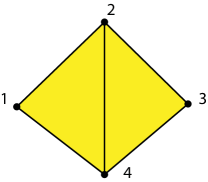
Figure 4: Illustration of example F.12. A simplicial complex.

Example F.12.

Consider the simplicial complex $L$ shown in Figure 4 and assume that $w^{L}\equiv 1$. Let $K$ be the subcomplex $\{[1],[2],[3],[4],[1,2],[2,3],[3,4],[1,4]\}$. Let $q_{0}=2$. Given the order $[1,2,3,4]$, it is easy to compute that

$$\boldsymbol{\Delta}_{1,\mathrm{up}}^{K,L}=\frac{1}{2}\begin{pmatrix}1&1&1&-1\\ 1&1&1&-1\\ 1&1&1&-1\\ -1&-1&-1&1\end{pmatrix}.$$

Therefore, for each $i=1,2,3,4$, we have that

$$\sum_{j\neq i}\big{|}\boldsymbol{\Delta}_{1,\mathrm{up}}^{K}(i,j)\big{|}=\frac{3}{2}=3\cdot\boldsymbol{\Delta}_{1,\mathrm{up}}^{K}(i,i)\neq q_{0}\cdot\boldsymbol{\Delta}_{1,\mathrm{up}}^{K}(i,i)$$

and thus there exists no well-defined simplicial network with $\boldsymbol{\Delta}_{1,\mathrm{up}}^{K,L}$ being its $1$-st up Laplacian.

References

- [1] João Carlos Alves Barata and Mahir Saleh Hussein. The Moore–Penrose pseudoinverse: A tutorial review of the theory. Brazilian Journal of Physics, 42(1-2):146–165, 2012.
- [2] Béla Bollobás. Modern graph theory. Graduate Texts in Mathematics. Springer-Verlag New York, 1998.
- [3] Oleksiy Busaryev, Sergio Cabello, Chao Chen, Tamal K Dey, and Yusu Wang. Annotating simplices with a homology basis and its applications. In Algorithm Theory - SWAT 2012 - 13th Scandinavian Symposium and Workshops, Helsinki, Finland, July 4-6, 2012. Proceedings, pages 189–200, 2012. doi:10.1007/978-3-642-31155-0\_17.
- [4] Peter Buser. A note on the isoperimetric constant. In Annales scientifiques de l’École Normale Supérieure, volume 15, pages 213–230, 1982.
- [5] David Carlson, Emilie Haynsworth, and Thomas Markham. A generalization of the Schur complement by means of the Moore–Penrose inverse. SIAM Journal on Applied Mathematics, 26(1):169–175, 1974.
- [6] Jeff Cheeger. A lower bound for the smallest eigenvalue of the Laplacian. In Proceedings of the Princeton conference in honor of Professor S. Bochner, pages 195–199, 1969.
- [7] Jiahui Chen, Rundong Zhao, Yiying Tong, and Guo-Wei Wei. Evolutionary de Rham-Hodge method. Discrete & Continuous Dynamical Systems-B, 22(11):0, 2017.
- [8] Fan RK Chung. Laplacians of graphs and Cheeger’s inequalities. Combinatorics, Paul Erdos is Eighty, 2(157-172):13–2, 1996.
- [9] Fan RK Chung. Spectral Graph Theory. Amer. Math. Soc., 1997.
- [10] Vin De Silva, Dmitriy Morozov, and Mikael Vejdemo-Johansson. Persistent cohomology and circular coordinates. Discrete & Computational Geometry, 45(4):737–759, 2011.
- [11] Florian Dorfler and Francesco Bullo. Kron reduction of graphs with applications to electrical networks. IEEE Transactions on Circuits and Systems I: Regular Papers, 60(1):150–163, 2012.
- [12] Peter G Doyle and J Laurie Snell. Random walks and electric networks, volume 22. American Mathematical Soc., 1984.
- [13] Art Duval and Victor Reiner. Shifted simplicial complexes are Laplacian integral. Transactions of the American Mathematical Society, 354(11):4313–4344, 2002.
- [14] Beno Eckmann. Harmonische funktionen und randwertaufgaben in einem komplex. Commentarii Mathematici Helvetici, 17(1):240–255, 1944.
- [15] Herbert Edelsbrunner, David Letscher, and Afra Zomorodian. Topological persistence and simplification. In Proceedings 41st annual symposium on foundations of computer science, pages 454–463. IEEE, 2000.
- [16] Yizheng Fan. Schur complements and its applications to symmetric nonnegative and Z-matrices. Linear algebra and its applications, 353(1-3):289–307, 2002.
- [17] J Friedrich, M Günther, L Klotz, et al. A generalized Schur complement for nonnegative operators on linear spaces. Banach Journal of Mathematical Analysis, 12(3):617–633, 2018.
- [18] Timothy E Goldberg. Combinatorial Laplacians of simplicial complexes. Senior Thesis, Bard College, 2002.
- [19] Anna Gundert and May Szedlák. Higher dimensional Cheeger inequalities. In Siu-Wing Cheng and Olivier Devillers, editors, 30th Annual Symposium on Computational Geometry (SoCG), page 181. ACM, 2014. doi:10.1145/2582112.2582118.
- [20] Anna Gundert and May Szedlák. Higher dimensional discrete Cheeger inequalities. Journal of Computational Geometry, 6(2), 2015.
- [21] Jakob Hansen. Laplacians of Cellular Sheaves: Theory and Applications. PhD thesis, University of Pennsylvania, 2020.
- [22] Jakob Hansen and Robert Ghrist. Toward a spectral theory of cellular sheaves. Journal of Applied and Computational Topology, 3(4):315–358, 2019.
- [23] Allen Hatcher. Algebraic topology. 2000.
- [24] Shlomo Hoory, Nathan Linial, and Avi Wigderson. Expander graphs and their applications. Bulletin of the American Mathematical Society, 43(4):439–561, 2006.
- [25] Danijela Horak and Jürgen Jost. Spectra of combinatorial Laplace operators on simplicial complexes. Advances in Mathematics, 244:303–336, 2013.
- [26] Palle ET Jorgensen and PJ Pearse Erin. Operator theory and analysis of infinite networks. arXiv preprint arXiv:0806.3881, 3, 2008.
- [27] Matthias Keller and Delio Mugnolo. General Cheeger inequalities for p-Laplacians on graphs. Nonlinear Analysis: Theory, Methods & Applications, 147:80–95, 2016.
- [28] Woojin Kim and Facundo Mémoli. Spatiotemporal persistent homology for dynamic metric spaces. Discrete & Computational Geometry, pages 1–45, 2020.
- [29] Woong Kook and Kang-Ju Lee. Simplicial networks and effective resistance. Advances in Applied Mathematics, 100:71–86, 2018.
- [30] Ioannis Koutis, Gary Miller, and Richard Peng. A fast solver for a class of linear systems. Communications of the ACM, 55, 2012.
- [31] Gabriel Kron. Tensor analysis of networks. New York, 1939.
- [32] VI Lebedev and VI Agoshkov. Poincaré-Steklov operators and their applications in analysis. Computer Center of the USSR Academy of Sciences, Moscow, 1983.
- [33] James R Lee, Shayan Oveis Gharan, and Luca Trevisan. Multiway spectral partitioning and higher-order Cheeger inequalities. Journal of the ACM (JACM), 61(6):1–30, 2014.
- [34] James R Lee, Shayan Oveis Gharan, and Luca Trevisan. Multi-way spectral partitioning and higher-order Cheeger inequalities. In Symposium on Theory of Computing (STOC), pages 1117–1130, 2012.
- [35] André Lieutier. Talk: Persistent harmonic forms. URL: https://project.inria.fr/gudhi/files/2014/10/Persistent-Harmonic-Forms.pdf.
- [36] Lek-Heng Lim. Hodge Laplacians on graphs. Siam Review, 62(3):685–715, 2020.
- [37] Oren E Livne and Achi Brandt. Lean algebraic multigrid (lamg): Fast graph Laplacian linear solver. SIAM Journal on Scientific Computing, 34(4):B499–B522, 2012.
- [38] Russell Lyons and Yuval Peres. Probability on trees and networks, volume 42. Cambridge University Press, 2017.
- [39] Russell Lyons, Yuval Peres, Xin Sun, et al. Induced graphs of uniform spanning forests. In Annales de l’Institut Henri Poincaré, Probabilités et Statistiques, volume 56, pages 2732–2744. Institut Henri Poincaré, 2020.
- [40] Anne Marsden. Eigenvalues of the Laplacian and their relationship to the connectedness of a graph. University of Chicago, REU, 2013.
- [41] Roy Meshulam and Nathan Wallach. Homological connectivity of random k-dimensional complexes. Random Structures & Algorithms, 34(3):408–417, 2009.
- [42] Facundo Mémoli, Zhengchao Wan, and Yusu Wang. Persistent laplacian: Github repository. https://github.com/ndag/Persistent-Laplacian, 2021.
- [43] Andrew Y Ng, Michael I Jordan, and Yair Weiss. On spectral clustering: Analysis and an algorithm. Advances in Neural Information Processing Systems, 14(2):849–856, 2002.
- [44] Braxton Osting, Sourabh Palande, and Bei Wang. Towards spectral sparsification of simplicial complexes based on generalized effective resistance. arXiv preprint arXiv:1708.08436, 2017.
- [45] Jose A Perea. Multiscale projective coordinates via persistent cohomology of sparse filtrations. Discrete & Computational Geometry, 59(1):175–225, 2018.
- [46] Ville Puuska. Erosion distance for generalized persistence modules. Homology, Homotopy & Applications, 22(1), 2020.
- [47] Yue Song, David J Hill, and Tao Liu. On extension of effective resistance with application to graph Laplacian definiteness and power network stability. IEEE Transactions on Circuits and Systems I: Regular Papers, 66(11):4415–4428, 2019.
- [48] Daniel A Spielman and Nikhil Srivastava. Graph sparsification by effective resistances. SIAM Journal on Computing, 40(6):1913–1926, 2011.
- [49] Daniel A Spielman and Shang-Hua Teng. Nearly-linear time algorithms for graph partitioning, graph sparsification, and solving linear systems. In Proceedings of the thirty-sixth annual ACM symposium on Theory of computing, pages 81–90, 2004.
- [50] John Steenbergen, Caroline Klivans, and Sayan Mukherjee. A Cheeger-type inequality on simplicial complexes. Advances in Applied Mathematics, 56:56–77, 2014.
- [51] Nisheeth K Vishnoi. Lx = b: Laplacian solvers and their algorithmic applications. Found. Trends Theor. Comput. Sci., 8(1-2):1–141, 2013. doi:10.1561/0400000054.
- [52] Ulrike von Luxburg. A tutorial on spectral clustering. In Statistics and Computing, volume 17, pages 395–416, 2007.
- [53] Rui Wang, Duc Duy Nguyen, and Guo-Wei Wei. Persistent spectral graph. International Journal for Numerical Methods in Biomedical Engineering, page e3376, 2020.
- [54] Rui Wang, Rundong Zhao, Emily Ribando-Gros, Jiahui Chen, Yiying Tong, and Guo-Wei Wei. HERMES: Persistent spectral graph software. arXiv preprint arXiv:2012.11065, 2020.
- [55] Rui Wang, Rundong Zhao, Emily Ribando-Gros, Jiahui Chen, Yiying Tong, and Guo-Wei Wei. HERMES: Persistent spectral graph software: Github repository. https://github.com/wangru25/HERMES, 2020.
- [56] Xiaojin Zhu, Zoubin Ghahramani, and John D Lafferty. Semi-supervised learning using Gaussian fields and harmonic functions. In Proceedings of the 20th International conference on Machine learning (ICML-03), pages 912–919, 2003.
- [57] Afra Zomorodian and Gunnar Carlsson. Computing persistent homology. Discrete & Computational Geometry, 33(2):249–274, 2005.