Learning summary features of time series for likelihood free inference

Abstract

There has been an increasing interest from the scientific community in using likelihood-free inference (LFI) to determine which parameters of a given simulator model could best describe a set of experimental data. Despite exciting recent results and a wide range of possible applications, an important bottleneck of LFI when applied to time series data is the necessity of defining a set of summary features, often hand-tailored based on domain knowledge. In this work, we present a data-driven strategy for automatically learning summary features from univariate time series and apply it to signals generated from autoregressive–moving-average (ARMA) models and the Van der Pol Oscillator. Our results indicate that learning summary features from data can compete and even outperform LFI methods based on hand-crafted values such as autocorrelation coefficients even in the linear case.

1 Introduction

Bayesian inference on modern complex simulator models is in general a difficult task because the likelihood function of the model’s output is often difficult or impossible to obtain. A modern approach for bypassing such an obstacle is to use likelihood-free inference methods, in which a flexible function (e.g. a neural network) learns how to approximate the posterior distribution based on simulations over different parameters. This approach is also called simulation-based inference (SBI) and we refer the reader to [5] for a review on the topic and the Python package sbi for ready-to-use implementations [18].

A common step in SBI is to reduce the dimensionality of the observed data before approximating the posterior distribution. This is particularly relevant when working with time series data, for which descriptions based on a few meaningful parameters is standard practice. For instance, the autocorrelation function is a sufficient statistic for signals generated by Gaussian autoregressive–moving-average (ARMA) models and is, therefore, the ideal summary feature extractor. For signals generated by complex non-linear simulators, such as the Hodgkin-Huxley or Lotka-Volterra models, the summary features are usually chosen based on previous domain knowledge [15]. In this work, we propose a data-driven strategy that avoids tailoring summary statistics for each application.

Automatically learning summary features is a recurring theme in the SBI literature. Fearnhead et al. [8] present a regression scheme that approximates the posterior mean via a linear model and uses it as summary features for learning the posterior distribution. Partially exchangeable networks (PEN) [19] explores invariances in time series to learn a set of summary features with the same loss function as [8] and then approximates the posterior distribution using them. An important difference of our work is that we learn the summary statistics and the posterior distribution jointly, as done in [11] but with a different summary feature extractor.

In what follows, we present the architecture of our summary feature extractor and show its performance in approximating posterior distributions of linear and non-linear stochastic time series models.

2 Methods

The basic setup of Bayesian methods for SBI consists of a prior distribution $p(\boldsymbol{\theta})$ over the parameters and a stochastic simulator whose output for a given $\boldsymbol{\theta}_{i}$ is $\boldsymbol{x}_{i}\sim p(\boldsymbol{x}|\boldsymbol{\theta}_{i})$. Our goal is to determine the posterior distribution of $\boldsymbol{\theta}$ given an observed simulator output $\boldsymbol{x}_{0}\in\mathbb{R}^{n_{s}}$, which we denote $p(\boldsymbol{\theta}|\boldsymbol{x}_{0})$.

2.1 Posterior estimation with adaptive summary features

We define the summary feature extractor as a function $f_{\boldsymbol{\lambda}}:\mathbb{R}^{n_{s}}\to\mathbb{R}^{n_{f}}$ whose parameters $\boldsymbol{\lambda}$ can be learned from the data and use a probability density estimator $q_{\boldsymbol{\phi}}$ parametrized by $\boldsymbol{\phi}$ to approximate $p(\boldsymbol{\theta}|\boldsymbol{x})$. We have, therefore, that $p(\boldsymbol{\theta}|\boldsymbol{x}_{0})\approx q_{\boldsymbol{\phi}}(\boldsymbol{\theta}|f_{\boldsymbol{\lambda}}(\boldsymbol{x}_{0}))$.

The parameters $\boldsymbol{\phi}$ and $\boldsymbol{\lambda}$ are determined by jointly minimizing the Kullback-Leiber divergence between the true posterior distribution and our approximation, which can be rewritten as

$$\mathcal{L}(\boldsymbol{\phi},\boldsymbol{\lambda})=\mathbb{E}_{(\boldsymbol{x},\boldsymbol{\theta})\sim p(\boldsymbol{x},\boldsymbol{\theta})}\Big{[}-\log(q_{\boldsymbol{\phi}}(\boldsymbol{\theta}|f_{\boldsymbol{\lambda}}(\boldsymbol{x})))\Big{]}~{}.$$ (1)

The standard approach for minimizing (1) is to generate a set of paired samples $(\boldsymbol{\theta}_{i},\boldsymbol{x}_{i})\sim p(\boldsymbol{\theta},\boldsymbol{x})$ and use stochastic gradient descent to obtain a minimizer. However, we have observed superior results with sequential neural posterior estimation (SNPE-C) [11]. It consists of an $R$-step procedure in which $N$ paired samples are generated per iteration and used to obtain a sequence of approximations of $p(\boldsymbol{\theta}|\boldsymbol{x})$. SNPE-C’s particularity is that the data points generated on a given round $r$ are sampled from a posterior approximation obtained on round $r-1$ fixed with $\boldsymbol{x}=\boldsymbol{x}_{0}$. This leads to approximations which are targeted to better represent the posterior distribution associated with the observed data point. As a result, the approximation of $p(\boldsymbol{\theta}|\boldsymbol{x}_{0})$ after $R$ rounds is often better than with a single round and $N\times R$ simulations.

In all experiments below, $q_{\boldsymbol{\phi}}$ is a normalizing flow [14] with an autoregressive architecture implemented via the masked autoencoder for distribution estimation (MADE) [10]. We follow the same setup from [7] and [11] for LFI problems, stackings five MADEs, each with two hidden layers of 50 units, and a standard normal base distribution for the normalizing flow. This choice provides a sufficiently flexible function capable of approximating complex posterior distributions. We refer the reader to [13] for more information on the different types of normalizing flows. We run SNPE-C with $R=10$ rounds and $N=5000$ simulations per round.

2.2 The YuleNet

The summary feature extractor that we propose is based on a previously published neural network architecture presented in [4]. For an input time series realization $\boldsymbol{x}\in\mathbb{R}^{n_{s}}$ ($n_{s}>256$), we get an $n_{f}$-dimensional feature vector given by

$$f_{\boldsymbol{\lambda}}(\boldsymbol{x})=g_{3}\big{(}g_{2}\big{(}g_{1}(\boldsymbol{x})\big{)}\big{)}\in\mathbb{R}^{n_{f}}~{},$$ (2)

where $g_{1},g_{2},$ and $g_{3}$ are functions with trainable parameters,

• 1D CNN (input channels: 1, output channels: 8, kernel size: 64, stride: 1, padding: 32) followed by a ReLU activation function and an average pooling (kernel size: 16)

• 1D CNN (input channels: 8, output channels: 8, kernel size: 64, stride: 1, padding: 32) followed by a ReLU activation function and an average pooling (kernel size: $\lfloor n_{s}/256\rfloor$)

• 50%-dropout layer followed by a linear transformation with $n_{f}$-dimensional output and a ReLU activation function.

We name our summary feature extractor YuleNet in reference to the widely known Yule-Walker equations from time series analysis [6]. A YuleNet contains $4624+n_{f}(1+n_{s}/32)$ trainable parameters in total. In all of the examples considered in this paper, we have $n_{s}=4096$ and $n_{f}=5$, leading to 5269 parameters to optimize.

2.3 Examples on linear time series processes

We consider two examples on discrete-time series generated by stochastic linear models. Despite their simplicity, these models are good benchmarks for validating our approach since the posterior distributions are known analytically.

Our first example is an auto-regressive process of order two parametrized by $k_{1},k_{2}\in(-1,+1)$,

$$x(n)=(k_{1}+k_{1}k_{2})x(n-1)+|k_{2}|x(n-2)+u(n)~{},$$ (3)

where $u$ is a zero-mean discrete-time Gaussian white noise process with unit variance. Note that the absolute value taken over $k_{2}$ leads to a posterior distribution $\boldsymbol{\theta}=(k_{1},k_{2})$ which has two modes. We call this example bimodal-AR(2). Our second example is a moving-average process of order two, MA(2):

$$x(n)=(k_{1}+k_{1}k_{2})\epsilon(n-1)+k_{2}\epsilon(n-2)+u(n)~{},$$ (4)

with $k_{1},k_{2},$ and $u$ defined as in (3). Note that the parametrization in terms of $k_{1},k_{2}$ ensures that bimodal-AR(2) is a stationary process and that MA(2) is an invertible process [3].

In both examples, we use SNPE-C to approximate the posterior distribution $p(\boldsymbol{\theta}|\boldsymbol{x}_{0})$ with $\boldsymbol{x}_{0}$ generated by $\boldsymbol{\theta}_{0}=(k_{1},k_{2})=(0.5,-0.75)$. We consider an uniform prior distribution for the parameters $k_{1},k_{2}\sim\mathcal{U}(-1,+1)$.

2.4 The Van der Pol oscillator

The Van der Pol oscillator (VdPOsc) is a non-linear system widely known in the study of chaotic systems. It has been used to decribe different phenomena in physics, biology, and electrical engineering [17]. In this example, we consider a stochastic version driven by a random process [1]. For a continuous time series $x(t)$, we have

$$\ddot{x}=\varepsilon(1-x^{2})\dot{x}-x+\sigma\dot{w}~{},$$ (5)

where $\varepsilon>0$ and $\sigma>0$, and $\dot{w}(t)$ is a Gaussian white noise of zero mean and unit variance.

We solve (5) using a Euler-Maruyama solver for Ito equations with $\Delta t=0.01s$ and then downsample the time series to a sampling period of $T_{s}=0.05s$. The initial conditions are fixed to $(x(0),\dot{x}(0))=(1.0,2.0)$. We use SNPE-C to approximate the posterior distribution $p(\boldsymbol{\theta}|\boldsymbol{x}^{(i)}_{0})$ with ${\boldsymbol{\theta}}=(\varepsilon,\sigma)$ in five different cases:

$$\begin{array}[]{ccccc}\boldsymbol{\theta}^{(1)}_{0}=(2.5,1.0)&\boldsymbol{\theta}^{(3)}_{0}=(1.0,1.5)&\boldsymbol{\theta}^{(5)}_{0}=(4.0,0.5)&\boldsymbol{\theta}^{(2)}_{0}=(1.0,0.5)&\boldsymbol{\theta}^{(4)}_{0}=(4.0,1.5)\end{array}$$

We consider a prior distribution for $\varepsilon\sim\mathcal{U}(0,5)$ and $\sigma\sim\mathcal{U}(0,2)$.

3 Results and discussion

Examples with linear time series processes. We assess the quality of the results with SNPE-C via the Wasserstein distance [16] calculated over samples from the analytic and approximated posteriors of bimodal-AR(2) and MA(2). We compare the results obtained when the summary features are extracted via the YuleNet architecture to when they are estimates of the autocorrelations of the time series ( autocorr). Note that because $u$ is a Gaussian white noise in both (3) and (4), the autocorrelations are sufficient statistics, making them the ideal benchmark. We also consider a case where $f_{\boldsymbol{\lambda}}$ is a PEN with the same setup from [19] in two situations: when its parameters are learned within the SNPE-C procedure (PEN), and when they are learned separately on $10^{4}$ simulated samples and then applied to a rejection-sample ABC procedure (PEN+ABC) as done in [19].

Figure 1 shows that the Wasserstein distances of all methods decrease when the simulation budget increases (simulation budget = round number $\times$ simulations per round). In bimodal-AR(2), the performances of autocorr, YuleNet, and PEN are very similar, whereas PEN+ABC is slightly worse. It is worth mentioning that PEN has twice more parameters as compared to YuleNet (10285 versus 5269) and requires $\approx 27.10^{6}$ multiply-accumulate operations (MACs) per forward computation, against $\approx 3.10^{6}$ for YuleNet. In practice, we have observed that the evaluations of PENs are between three and five times longer in CPU time than with YuleNet. In MA(2), we observe that YuleNet and PEN are uniformly better than autocorr, indicating that the learned summary features in this case are better representations of the time series for the inference procedure than the estimated autocorrelations. This can be explained by the highly complex relation between the theoretical values of the autocorrelations of MA(2) and parameters $k_{1}$ and $k_{2}$, which makes the model inversion via SNPE-C very difficult (see Appendix 5 for details).

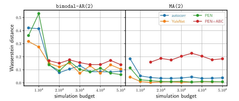
Figure 1: Wasserstein distance between the estimated posterior and the analytical posterior distribution for the examples on linear time series processes. The distances have been averaged over 100 batches with 100 samples from each posterior distribution (all calculations done with the POT package [9])

Results on the Van der Pol oscillator. We are not aware of any direct method for obtaining samples of the true posterior distribution of VdPOsc. Therefore, we base our discussion on the inspection of 2D histograms of the samples from each approximation to $p(\boldsymbol{\theta}|\boldsymbol{x}_{0})$. We consider results only for autocorr and YuleNet.

The left and center plots of Figure 2 show that the posterior distribution approximated with autocorr generates samples which are very far from the ground truth parameter, whereas YuleNet yields sharp posterior distributions around the true parameter. This indicates that using only autocorrelations as summary features for a non-linear model such as VdPOsc is not sufficient to capture its statistical properties and that the flexibility of YuleNet allows for a better representation of the time series. We also observe that the dispersions of the samples of the posterior distributions obtained for YuleNet vary for different ground truth parameters: the standard deviation $\sigma$ of the input Gaussian white noise has the usual effect of increasing the variance of the posterior distribution, and the ‘degree’ of non-linearity of VdPOsc, modulated by $\varepsilon$, shows that when the system tends to an harmonic oscillator ($\varepsilon\to 0$) the posterior distribution has less variance. The four small plots on the right side of Figure 2 display how the dispersion of the samples from the posterior approximation vary for different lengths of the observed time series. They show that our approximate posterior has the expected behavior of getting sharper when longer observations are available.

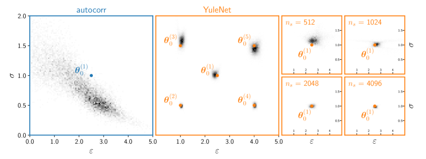
Figure 2: Results on the Van der Pol oscillator after ten SNPE-C rounds. The left plot portrays a 2D histogram of $10^{4}$ samples from the posterior distribution approximated with autocorr for ground truth parameter $\boldsymbol{\theta}^{(1)}_{0}$. It shows that autocorrelations are not adequate summary statistics for this example. The center plot shares the y-axis of the left plot and overlays the histograms from approximations estimated with YuleNet on five different ground truth parameters ($10^{4}$ samples for each case). We see how the shape of the posterior distribution varies for different choices of ground truth parameter $\boldsymbol{\theta}^{(i)}_{0}$. The four small plots on the right demonstrate that the dispersion of the samples with YuleNet decrease when longer time series are used in the inference procedure.

4 Conclusion

Our experiments have demonstrated that data-driven summary features of time series learnt for SBI can match the performance of sufficient statistics in the Gaussian linear case, while being significantly better on a non-linear stochastic model. The YuleNet architecture that we present, which is simply a well calibrated one-dimensional CNN, learns adequate summary features for inference while using less parameters and requiring less computational power (measured via MACs) to train than another proposal from the literature. Using the SNPE-C procedure to minimize (1) and a normalizing flow for $q_{\boldsymbol{\phi}}$ has given satisfactory results, but other options are possible too, such as using MDNs [2] to approximate probability distributions and employing other LFI strategies as in [15] and [12].

Broader Impact

Inferring the laws and parameters that drive physical systems has been a long standing issue in physics, and more broadly across all experimental sciences. In this work, we have presented a method for automatically determining summary statistics from experimental time series and used them with a LFI method to obtain the parameters of a simulator model. Our main contribution is in easing the burden on specialists interested in applying LFI in practice, since the tailoring of summary statistics for each application is often time consuming.

5 Appendix

The auto-correlation function for bimodal-AR(2) in terms of $(k_{1},k_{2})$ is

$$r(1)=\frac{k_{1}+k_{1}|k_{2}|}{1-|k_{2}|}~{},~{}r(2)=|k_{2}|+\frac{(k_{1}+k_{1}|k_{2}|)^{2}}{1-|k_{2}|}~{},$$ (6)

and $r(s)=a_{1}r(s-1)+a_{2}r(s-2),\forall s>2,s\in\mathbb{Z}$. The auto-correlation function for MA(2) is

$$\quad r(1)=\frac{(k_{1}+k_{1}k_{2})(1+k_{2})}{1+(k_{1}+k_{1}k_{2})^{2}+k_{2}^{2}}\quad\text{and}\quad r(2)=\frac{k_{2}}{1+(k_{1}+k_{1}k_{2})^{2}+k_{2}^{2}}~{},$$ (7)

and $r(s)=0,\forall s>2,s\in\mathbb{Z}$. When using autocorrelations as summary features, the SNPE-C procedure learns to invert these relations and obtain the values of $k_{1}$ and $k_{2}$ in terms of $r(k)$.

References

- [1] Roman Belousov, Florian Berger, and A. J. Hudspeth. Volterra-series approach to stochastic nonlinear dynamics: Linear response of the van der pol oscillator driven by white noise. Phys. Rev. E, 102:032209, Sep 2020.
- [2] Christopher M. Bishop. Mixture density networks. Technical report, 1994.
- [3] George.E.P. Box and Gwilym M. Jenkins. Time Series Analysis: Forecasting and Control. Holden-Day, 1976.
- [4] Stanislas Chambon, Mathieu N. Galtier, Pierrick J. Arnal, Gilles Wainrib, and Alexandre Gramfort. A Deep Learning Architecture for Temporal Sleep Stage Classification Using Multivariate and Multimodal Time Series. IEEE Transactions on Neural Systems and Rehabilitation Engineering, 26(4):758–769, 2018.
- [5] Kyle Cranmer, Johann Brehmer, and Gilles Louppe. The frontier of simulation-based inference. Proceedings of the National Academy of Sciences, 2020.
- [6] James Durbin. The fitting of time-series models. Review of the Int. statistical institute, pages 233–244, 1960.
- [7] Conor Durkan, Iain Murray, and George Papamakarios. On contrastive learning for likelihood-free inference, 2020.
- [8] Paul Fearnhead and Dennis Prangle. Constructing summary statistics for approximate bayesian computation: semi-automatic approximate bayesian computation. Journal of the Royal Statistical Society: Series B (Statistical Methodology), 74(3):419–474, 2012.
- [9] Rémi Flamary and Nicolas Courty. POT Python Optimal Transport library, 2017.
- [10] Mathieu Germain, Karol Gregor, Iain Murray, and Hugo Larochelle. MADE: Masked Autoencoder for Distribution Estimation. volume 37 of Proceedings of Machine Learning Research, pages 881–889, Lille, France, 07–09 Jul 2015. PMLR.
- [11] David Greenberg, Marcel Nonnenmacher, and Jakob Macke. Automatic posterior transformation for likelihood-free inference. volume 97 of Proceedings of Machine Learning Research, pages 2404–2414, Long Beach, California, USA, 09–15 Jun 2019. PMLR.
- [12] Joeri Hermans, Volodimir Begy, and Gilles Louppe. Likelihood-free mcmc with amortized approximate ratio estimators, 2020.
- [13] George Papamakarios, Eric Nalisnick, Danilo Jimenez Rezende, Shakir Mohamed, and Balaji Lakshminarayanan. Normalizing flows for probabilistic modeling and inference, 2019.
- [14] George Papamakarios, Theo Pavlakou, and Iain Murray. Masked autoregressive flow for density estimation. In I. Guyon, U. V. Luxburg, S. Bengio, H. Wallach, R. Fergus, S. Vishwanathan, and R. Garnett, editors, Advances in Neural Information Processing Systems 30, pages 2338–2347. Curran Associates, Inc., 2017.
- [15] George Papamakarios, David Sterratt, and Iain Murray. Sequential neural likelihood: Fast likelihood-free inference with autoregressive flows. volume 89 of Proceedings of Machine Learning Research, pages 837–848. PMLR, 16–18 Apr 2019.
- [16] Gabriel Peyré and Marco Cuturi. Computational optimal transport: With applications to data science. Foundations and Trends® in Machine Learning, 11(5-6):355–607, 2019.
- [17] Steven H. Strogatz. Nonlinear Dynamics and Chaos: With Applications to Physics, Biology, Chemistry and Engineering. Westview Press, 2000.
- [18] Alvaro Tejero-Cantero, Jan Boelts, Michael Deistler, Jan-Matthis Lueckmann, Conor Durkan, Pedro J. Gonçalves, David S. Greenberg, and Jakob H. Macke. sbi: A toolkit for simulation-based inference. Journal of Open Source Software, 5(52):2505, 2020.
- [19] Samuel Wiqvist, Pierre-Alexandre Mattei, Umberto Picchini, and Jes Frellsen. Partially exchangeable networks and architectures for learning summary statistics in approximate Bayesian computation. volume 97 of Proceedings of Machine Learning Research, pages 6798–6807, Long Beach, California, USA, 09–15 Jun 2019. PMLR.