A Multivariate Realized GARCH Model

Abstract

We propose a novel class of multivariate GARCH models that utilize realized measures of volatilities and correlations. The central component is an unconstrained vector parametrization of the correlation matrix that facilitates modeling of the correlation structure. The parametrization is based on the matrix logarithmic transformation that retains the positive definiteness as an innate property. A factor approach offers a way to impose a parsimonious structure in high dimensional system and we show that a factor framework arises naturally in some existing models. We apply the model to returns of nine assets and employ the factor structure that emerges from a block correlation specification. An auxiliary empirical finding is that the empirical distribution of parametrized realized correlations is approximately Gaussian. This observation is analogous to the well-known result for logarithmically transformed realized variances.

Keywords: Financial Volatility, Realized GARCH, High Frequency Data, Multivariate Modeling, Correlation matrix, Matrix logarithm.

JEL Classification: G11, G17, C32, C58

1 Introduction

Univariate GARCH models have had much empirical success since the ARCH model was introduced by Engle, (1982). A large number of univariate GARCH-type models have been proposed in the literature, whereas the literature on multivariate GARCH models is less voluminous. A key obstacle in multivariate extensions is that it is not entirely obvious how the univariate GARCH structure is naturally generalized to higher dimensions. The main object of interest is the conditional covariance matrix, $H_{t}=\mathrm{var}(r_{t}|\mathcal{F}_{t-1})$, and there are two main challenges to modeling $H_{t}$ in the multivariate setting. First, a model must produce a positive (semi) definite matrix, and this entails nonlinear cross restrictions on the elements of $H_{t}$. Second, the number of covariance terms for a vector of dimension $p$ is proportional to $p^{2}$, and this can become computationally difficult, unless $p$ is relatively small. Many multivariate GARCH models impose a structure on $H_{t}$ that serves to address these two issues. A convenient way to model $H_{t}$, which we adopt in this paper, is to separately model variances and correlations. This was the structure in the seminal paper by Bollerslev, (1990), who proposed the constant correlation model. It is also the structure in the Dynamic Conditional Correlation (DCC) model by Engle, 2002a , see also Engle and Sheppard, (2001), Shephard et al., (2020), Aielli, (2013), and Engle et al., (2019). In our empirical section, we explore the equicorrelation and the block correlation structures used in Engle and Kelly, (2012). Both these structures arise as special cases in our factor model for the correlation matrix, and our approach guarantees positive definiteness. We also make use of realized measures of volatilities and correlations, and provide some simplifications of the likelihood evaluation.

The main contributions in this paper are the following. First, we develop a new class of multivariate GARCH models that facilitates a flexible modeling of the correlation structure, while positive definiteness is assured without further constraints. The main methodological contribution is the dynamic model for the vector representation of the correlation matrix, and the simple factor structure this approach permits. The factor approach is helpful for reducing the number of free parameters/variables in the model. Second, we show that this factor structure arises naturally in models with equicorrelation and block correlation matrices. A block correlation structure may be motivated by the sector classifications of the individual assets, or some other appropriate categorization. Third, we demonstrate the usefulness of the framework in an empirical application with nine asset return series, where we explore a block correlation structure motivated by industry sectors the assets belong to. We find the new model structure improves the empirical fit both in-sample and out-of-sample when compared to simpler models, such as the constant correlation model and the equicorrelation model. The predicted covariance matrices can be used for optimal portfolio construction, and portfolio variance is reduced by a factor of two relative to a naive equal-weights portfolio. Fourth, we make an interesting auxiliary empirical observation. We find the vector representation of the realized correlation matrix is approximately Gaussian distributed. This result is analogous to existing results for the logarithmically transformed realized variances, see Andersen et al., 2001a . These two empirical findings provide justification for the Gaussian specification we use in our construction of the likelihood function.

The new class of multivariate GARCH models is based on a convenient parametrization of the conditional correlation matrix, $C_{t}$, that corresponds to $H_{t}$. The parametrization is given by the vector $\varrho_{t}=g(C_{t})$, where the mapping $\varrho=g(C)$ is defined by taking the matrix logarithm to the correlation matrix, $C$, and stacking the off-diagonal elements of $\log C$ into the vector $\varrho\in\mathbb{R}^{d}$, where $d=p(p-1)/2$. This parametrization was recently introduced by Archakov and Hansen, 2020b , who showed that it has many interesting properties. For instance, this mapping is one-to-one between the set of non-singular correlation matrices and $\mathbb{R}^{d}$, so regardless of how the vector $\varrho_{t}$ is modeled or regulated, it will always map back to a unique positive definite correlation matrix. In other words, this parametrization guarantees positive definiteness, without imposing additional restrictions on $H_{t}$. It is, however, straightforward to impose additional structure on the correlation matrix, if required. A more parsimonious structure on $H_{t}$ is typically needed unless $p$ is small, and this can be achieved with a factor structure for $\varrho_{t}$, as we will show in Section 2.3. One situation where a factor structure for $\varrho_{t}$ emerges naturally, is when the correlation matrix has a block structure with identical correlations within each block.

Early multivariate GARCH models solely relied on daily returns in the dynamics of volatility. In this paper we also make use of realized measures of volatilities and correlations. This is beneficial, because the realized measures provide accurate signals about volatility, which is valuable in the dynamic modeling of conditional variances and correlations. The use of realized measures was popularized by results in Andersen and Bollerslev, (1998), and key theoretical results were subsequently established in Andersen et al., 2001b , Barndorff-Nielsen and Shephard, 2002a , Andersen et al., (2003), Barndorff-Nielsen and Shephard, 2004a , see also Hansen and Lunde, (2011) and references therein. Realized measures were initially used to evaluate the performance of GARCH models, see Andersen and Bollerslev, (1998). A natural next step was to incorporate realized measures in GARCH models and Engle, 2002b was one of the first to include realized measures as an exogenous variable in GARCH models. Complete models, that also specify a model for the realized measures, soon followed, including the MEM by Engle and Gallo, (2006), the HEAVY model by Shephard and Sheppard, (2010), and the Realized GARCH model by Hansen et al., (2012). Multivariate extensions of these models were proposed in Noureldin et al., (2012), Hansen et al., (2014), Dumitrescu and Hansen, (2017), and Gorgi et al., (2019). Another way to incorporate realized measures in multivariate GARCH models is explored in Bauwens et al., (2012), who build on the Conditional Autoregressive Wishart model of Golosnoy et al., (2012).

Our approach to modeling correlations could, with some adaptation, be implemented in a conventional manner, using daily returns only. However, it is more advantageous to include realized measures in the modeling. Realized measures are computed with high frequency data, and these provide accurate signals about the key components of the model. Including realized measures in a GARCH model makes it more responsive to sudden shifts in volatilities and correlations, which improve the empirical fit and model predictions, see Hansen and Huang, (2016). The Realized GARCH framework makes it easy to incorporate realized measures of volatility in the modeling. The model proposed in this paper is the first multivariate generalization of the Realized GARCH framework that makes it easy to incorporate realized measures of correlations without imposing additional restrictions on the covariance structure, besides positive definiteness.

The parametrization of the correlation matrix, $C_{t}$, involves the matrix logarithm of $C_{t}$. The matrix logarithm has previously been used in the modeling of covariance matrices in Chiu et al., (1996). In the context of the multivariate GARCH, it was used in Kawakatsu, (2006), and Asai and So, (2015) applied it to the DCC model. The transformation has also been used in stochastic volatility models, see Ishihara et al., (2016), and in reduced-form models of realized covariance matrices, see e.g. Bauer and Vorkink, (2011) and Weigand, (2014). Here we apply the matrix logarithm to the correlation matrix, which differs from applying it to the covariance matrix in important ways, see Archakov and Hansen, 2020b . In the present context, it enables us to model the conditional variances separately from the conditional correlations using a familiar GARCH structure for each of the univariate conditional variances. Moreover, this framework enables us to explicitly model the empirically important leverage effect.

We proceed as follows. In Section 2, we introduce notation, present the modeling framework, and discuss how a factor structure can be imposed on the correlation matrix. Section 3 details the estimation of the model and how the model can be used for forecasting. An extensive empirical analysis with nine asset returns series from three economic sectors is presented in Section 4. We conclude in Section 5 and complete the paper with two appendices with step-by-step directions on model estimation and additional empirical results, respectively.

2 The Multivariate Realized GARCH Model

In this section, we present the multivariate GARCH model that can utilize realized measures of variances and correlations. The key novelty is the way in which the correlation structure is modeled. We adopt a convenient reparametrization of the correlation matrix, recently proposed in Archakov and Hansen, 2020b . This vector representation, $\varrho_{t}=g(C_{t})$, does not impose any structure on $C_{t}$ beyond positive definiteness. Our methodological contribution is to propose a multivariate GARCH model that is based on $\varrho_{t}$, and develop a simple factor model for $\varrho_{t}$. We show a block correlation model corresponds to a particular factor structure, and we contribute to the literature on block correlation models by simplifying some expressions in the log-likelihood function.

2.1 Notation and Preliminaries

We let $r_{t}$ denote a $p$-dimensional vector of returns in period $t$, where $t$ represents a generic unit of time – typically a trading day. The conditional mean is denoted by $\mu_{t}=\mathbb{E}(r_{t}|\mathcal{F}_{t-1})$ and the conditional variance by

$$H_{t}=\mathrm{var}(r_{t}|\mathcal{F}_{t-1}),$$

where $\{\mathcal{F}_{t}\}$ is the natural filtration for $(r_{t},\mathrm{RM}_{t})$. Here $\mathrm{RM}_{t}$ denotes an ex-post empirical measure of $H_{t}$, such as the realized variance matrix, see Barndorff-Nielsen and Shephard, 2004b , or the multivariate realized kernel, see Barndorff-Nielsen et al., (2011).

Following Engle, 2002a , we decompose the conditional covariance matrix into variances and correlations,

$$H_{t}=\Lambda_{h_{t}}^{1/2}C_{t}\Lambda_{h_{t}}^{1/2},$$ (1)

where $\Lambda_{h_{t}}=\mathrm{diag}(h_{1,t},\ldots,h_{p,t})$ with $h_{i,t}=[H_{t}]_{ii}$, $i=1,\ldots,p$. Thus $h_{i,t}$ is the conditional variance of $r_{i,t}$ (the $i$-th element of $r_{t}$) and $C_{t}=\mathrm{corr}(r_{t}|\mathcal{F}_{t-1})$ is the conditional correlation matrix of $r_{t}$. The structure in (1) is the basis for the Dynamic Conditional Correlation framework, see Engle, 2002a and Engle and Sheppard, (2001). This formulation enables us to disentangle the dynamic properties of the conditional variances from that of the conditional correlations. In contrast to the conventional DCC model, we will incorporate realized measures of variances and correlations into the modeling, and we employ a different parametrization of $C_{t}$, which we detail below.

The central element in GARCH models is the equation that specifies the dynamic properties of $H_{t}$ and how these are influenced by lagged returns. This equation can be enhanced to include realized measures of volatility. The Realized GARCH model is characterized by a measurement equation that specifies how the realized measures are related to the contemporaneous conditional moments, such as $H_{t}$.

In this paper, we separate the modeling of $H_{t}$ in two parts: the modeling of the conditional variances and the modeling of the conditional correlations. This leads to two sets of GARCH and measurement equations, that utilize the appropriate realized measures. From $\mathrm{RM}_{t}\in\mathbb{R}^{p\times p}$, a positive definite realized measure of the covariance matrix in period $t$, we extract the diagonal elements $x_{t}=\mathrm{diag}(\mathrm{RM}_{t})$ and the corresponding correlation matrix denoted by

$$Y_{t}=\Lambda_{x_{t}}^{-1/2}\mathrm{RM}_{t}\Lambda_{x_{t}}^{-1/2}.$$

Here $\Lambda_{x_{t}}=\mathrm{diag}(x_{1,t},\ldots,x_{p,t})$ denotes the diagonal matrix with the elements of $x_{t}$ on the diagonal, and $Y_{t}$ inherits the positive definiteness from $\mathrm{RM}_{t}$. In summary, $x_{t}$ and $Y_{t}$ are the observed empirical measures of the latent variables, $h_{t}$ and $C_{t}$, respectively, and these will be used to inform the model about time variation in the latent variables. The realized measure, $\mathrm{RM}_{t}$, is typically consistent for the quadratic variation. The quadratic variation is not identical to the conditional variance, $H_{t}$, so we should expect non-trivial measurement errors in regard to how $x_{t}$ and $Y_{t}$ relate to $h_{t}$ and $C_{t}$, respectively.

We let $I_{n}$ denote the $n\times n$ identity matrix, and let $1_{\{\cdot\}}$ denotes the indicator function that equals one, if the expression within the curly brackets is true, and zero otherwise.

2.1.1 Parametrizing the Correlation Matrix

A symmetric matrix, $C_{t}$, needs to satisfy two properties in order to be a proper correlation matrix: it must be positive definite and each of its diagonal elements must be equal to one. Some approaches to modeling covariance matrices, satisfy these two requirements by imposing even stronger conditions. For instance, an equicorrelation structure with a single common correlation, $\rho$, satisfies both properties for $\rho\in(-\frac{1}{p-1},1)$, but also impose a very restrictive structure on the correlation matrix.

In this paper, we adopt a vector representation of the correlation matrix that was proposed by Archakov and Hansen, 2020b . This parametrization is based on the following mapping:

$$\varrho=g(C)=\mathrm{vecl}(\log C),$$

where $\log C$ is the matrix logarithmically transformed correlation matrix, and $\mathrm{vecl}(\cdot)$ extracts and vectorizes the elements below the diagonal. To illustrate this parametrization, consider the following example,

$$g\left(\left[\begin{array}[]{ccc}1.0&\bullet&\bullet\\ 0.8&1.0&\bullet\\ 0.0&0.2&1.0\end{array}\right]\right)=\mathrm{vecl}\log\left[\begin{array}[]{ccc}1.0&\bullet&\bullet\\ 0.8&1.0&\bullet\\ 0.0&0.2&1.0\end{array}\right]=\mathrm{vecl}\left[\begin{array}[]{ccc}-0.53&\bullet&\bullet\\ 1.14&-0.57&\bullet\\ -0.13&0.28&-0.03\end{array}\right]=\left(\begin{array}[]{c}1.14\\ -0.13\\ 0.28\end{array}\right).$$

In Archakov and Hansen, 2020b , it is shown that $g(C)$ is a one-to-one mapping between $\mathcal{C}_{p}$ and $\mathbb{R}^{d}$, where $\mathcal{C}_{p}$ is the space of positive definite $p\times p$ correlation matrices and $d=p(p-1)/2$. Thus, a non-singular $p\times p$ correlation matrix can be represented and modeled as a vector in $\mathbb{R}^{p(p-1)/2}$. In the bivariate case, $p=2$, where $C_{11}=C_{22}=1$ and $C_{12}=C_{21}=\rho$, it can be shown that $g(C)=\frac{1}{2}\log\frac{1-\rho}{1+\rho}$ , which is the Fisher transformation of the correlation coefficient, $\rho$. So $g(C)$ can be interpreted as a multivariate generalization of the Fisher transformation. In this case, the inverse transformation is available in a closed form, because $\rho=(e^{2\varrho}-1)/(e^{2\varrho}+1)$. In the general case, for arbitrary dimensions, $p$, the inverse mapping, $C=g^{-1}(\varrho)$, is given from a fast algorithm.

Having introduced the transformed conditional correlations, $\varrho_{t}=g(C_{t})$, we denote the corresponding transformed realized correlations by,

$$y_{t}=g(Y_{t}).$$

Both $\varrho_{t}$ and $y_{t}$ are $p(p-1)/2$-dimensional vectors. Instead of modeling the conditional correlation matrix, $C_{t}$, that is subject to positive (semi-) definite constraints, we will model the vector $\varrho_{t}$ that varies freely in $\mathbb{R}^{p(p-1)/2}$. The corresponding empirical measures are subjected to the same transformation, and $y_{t}$ is the empirical measure that we use to model the dynamic properties of $\varrho_{t}$. Much like the way that squared returns are used to model the conditional variance dynamics in a standard GARCH model.

The model presented above can be viewed as a natural generalization of the bivariate structure in Hansen et al., (2014), because the two models coincide when $p=2$, in which case $\varrho_{t}$ emerges as the Fisher transformed correlation. To form a model for a larger system, with $p>2$, the approach in Hansen et al., (2014) is to fuse bivariate models together to form a larger system. The fusing of bivariate models imply a (restricted) single-factor structure on $C_{t}$, which is not imposed by the model structure we propose in this paper.

2.2 The Model

With the required notation in place, we are now ready to introduce the multivariate realized GARCH model which consists of return equations, GARCH equations, and measurement equations. The return equation for the $i$-th asset at time $t$ takes the form

$$r_{i,t}=\mu_{i}+h_{i,t}^{1/2}z_{i,t},\qquad i=1,\ldots,p,\quad t=1,\ldots,T.$$

We have here assumed that $\mathbb{E}(r_{i,t}|\mathcal{F}_{t-1})=\mu_{i}$ is constant, as is often done in GARCH models. It follows that the standardized return $z_{i,t}=h_{i,t}^{-1/2}(r_{i,t}-\mu_{i})$ is such that $\mathbb{E}(z_{i,t}|\mathcal{F}_{t-1})=0$ and $\mathrm{var}(z_{i,t}|\mathcal{F}_{t-1})=1$. However, the standardized returns, $z_{t}=\Lambda_{h_{t}}^{-1/2}(r_{t}-\mu)$, are not uncorrelated since $\mathrm{var}(z_{t}|\mathcal{F}_{t-1})=C_{t}$. In our likelihood estimation, we assume $z_{t}$, $t=1,\dots,T$, to be distributed as i.i.d.$N(0,C_{t})$.

Next, we specify the GARCH equations that describe how $H_{t}$ depends on past observable variables. We make use of lagged values of standardized returns, $z_{t-1}$, and lagged values of realized measures, $x_{t-1}$ and $y_{t-1}$. The dynamics for the vector of conditional variances and the vector representation of the conditional correlations are as follows:

$$\log h_{t} =\omega+\beta\log h_{t-1}+\tau(z_{t-1})+\gamma\log x_{t-1},$$ (2)

$$\varrho_{t} =\tilde{\omega}+\tilde{\beta}\varrho_{t-1}\qquad\qquad\qquad+\tilde{\gamma}y_{t-1},$$

where $\omega$ is a $p\times 1$ vector, $\beta$ and $\gamma$ are $p\times p$ matrices, $\tau(\cdot)$ is a leverage function (which we elaborate on below, $\tilde{\omega}$ is a $d\times 1$ vector, while $\tilde{\beta}$ and $\tilde{\gamma}$ are $d\times d$ matrices where $d=p(p-1)/2$.

Realized GARCH models are characterized by measurement equations that relate latent conditional variables to their contemporaneous empirical quantities. In the present context, where we have realized measures of variances and the (transformed) correlations, and we adopt the following measurement equations:

$$\log x_{t} =\xi+\Phi\log h_{t}+\delta(z_{t})+v_{t},$$ (3)

$$y_{t} =\tilde{\xi}+\tilde{\Phi}\varrho_{t}+\tilde{v}_{t},$$

where $\xi$ is a $p\times 1$ vector, $\Phi$ is a $p\times p$ matrix, $\tilde{\xi}$ is a $d\times 1$ vector, $\tilde{\Phi}$ is a $d\times d$ matrix, and $\delta(\cdot)$ is (like $\tau(\cdot)$) a leverage function that captures dependencies between return and volatility innovations. This dependency is known to be empirically important, and is often referred to as the leverage effect, see Black, (1976), Christie, (1982), Engle and Ng, (1993). In our empirical analysis, we simplify the structure further by specifying the matrices $\beta,$ $\tilde{\beta},$ $\gamma$, $\tilde{\gamma}$, $\Phi$, and $\tilde{\Phi}$ to be diagonal matrices.

The measurement equations involve the “error” terms $v_{t}$ and $\tilde{v}_{t}$, which we stack into the vector $u_{t}=(v_{t}^{\prime},\tilde{v}_{t}^{\prime})^{\prime}$. In our likelihood analysis, we specify $u_{t}$ to be i.i.d.$N(0,\Sigma)$ and independent of $z_{t}$. The Gaussian specification is less likely to be at odds with data because the measurement equations are formulated with the logarithmically transformed variances, $\log x_{t}$, and the transformed correlations, $y_{t}=g(Y_{t})$. For instance, Andersen et al., 2001a and Barndorff-Nielsen and Shephard, 2002b found that the logarithm of the realized variance can be well approximated by a Gaussian distribution. Furthermore, we found evidence that $y_{t}$ is approximately Gaussian distributed, as is the case for $\log x_{t}$, which adds empirical support for adopting a Gaussian specification for the likelihood function. The empirical justification for the Gaussian specification will be presented in Section 4.3.

The measurement errors are likely to be correlated in practice, so the covariance matrix $\Sigma$ is not expected to be a diagonal matrix. The assumption that $u_{t}$ and $z_{t}$ are independent is obviously restrictive, however, the inclusion of the leverage function, $\delta(\cdot)$, serves to eliminate some forms of dependencies. The leverage function is sought to capture the conditional mean, $\delta(z_{t})=\mathbb{E}[\log x_{t}-\xi-\Phi\log h_{t}|z_{t}]$, which would imply mean-independence, $\mathbb{E}[u_{t}|z_{t}]=0$. We adopt the parametric leverage function given by,

$$\delta(z_{t})=\delta_{1}z_{t}+\delta_{2}(z_{t}\circ z_{t}-\iota_{p}),$$

where $\iota_{p}$ denotes the $p\times 1$ vector of ones, $\delta_{1}$ and $\delta_{2}$ are $p\times p$ coefficient matrices. This leverage function defines a multivariate version of the leverage function introduced in Hansen et al., (2012). We parametrize $\tau$ similarly, $\tau(z)=\tau_{1}z+\tau_{2}(z\circ z-\iota_{p})$, where $\tau_{1}$ and $\tau_{2}$ are $p\times p$ matrices. This structure is motivated by results in Hansen et al., (2012) and Hansen and Huang, (2016) who found that a parsimonious leverage function written as a second-order Hermite polynomial is sufficient for capturing the asymmetry dependence between return shocks and volatility shocks. In our empirical analysis, we also impose a diagonal matrix structure on the four $p\times p$ matrices $\delta_{1}$, $\delta_{2}$, $\tau_{1}$, and $\tau_{2}$, to reduce the number of free parameters in the model.

In the next Section, we discuss ways to further simplify the model by reducing the number of latent variables driving the dynamics of the correlation matrix.

2.3 A Factor Model for the Correlation Structure

The formulation above permits a flexible modeling of the correlation matrix. Any non-singular correlation matrix maps to a unique vector, and any vector (of proper dimension) maps to a unique correlation matrix. The number of latent variables embedded in the correlation matrix, $C_{t}$, is the dimension of $\varrho_{t}$, that equals $d(p)=p(p-1)/2$ . Thus $d(p)=1,3,6,10,15,21,28,36$, for $p=2,\ldots,9$, and the number of latent variables becomes unmanageable unless $p$ is relatively small. This necessitates that we impose additional structure on the model whenever $p$ is large.

We achieve this by modeling $\varrho_{t}$ with a factor structure, $\varrho_{t}=\varrho(\zeta_{t})$, where $\zeta_{t}$ is a lower dimensional vector of factors $\zeta_{t}\in\mathbb{R}^{k}$, $k<d$, so that $\varrho_{t}$ can be represented by a linear factor model,

$$\varrho_{t}=A\zeta_{t},$$

where $A$ is a $d\times k$ matrix. The implication is that the variation in $C_{t}$ is driven by $k$ factors, where the factors are the elements in $\zeta_{t}$. The linear structure makes it straightforward to reduce the dimension of the GARCH and measurement equations. The linear restriction is consistent with the lower dimensional GARCH equation,

$$\zeta_{t}=\check{\omega}+\check{\beta}\zeta_{t-1}+\check{\gamma}\check{y}_{t-1},$$ (4)

where $\check{y}_{t}=(A^{\prime}A)^{-1}A^{\prime}y_{t}\in\mathbb{R}^{k}$. That $\check{y}_{t}$ is the proper signal about $\zeta_{t}$ follows from well known projection arguments. The corresponding measurement equation is given by

$$\check{y}_{t}=\check{\xi}+\check{\Phi}\zeta_{t}+\check{v}_{t}.$$ (5)

So the linear restrictions enable us to reduce the dimension of both equations to $k$ from $d$.

The dimension reduction (outlined here) requires a $d\times k$ matrix, $A$. This matrix may be chosen ex-ante, but may also be determined empirically. An empirically estimated $A$ (or rather the subspace spanned by its columns) including the number of columns in $A$ (the number of factors), would require proper inference methods to be derived for this purpose. In this paper, we will focus on the case where $A$ is known, and leave the case with an empirically determined $A$ for future research. We also leave general, non-linear, factor structures, $\varrho_{t}=\varrho(\zeta_{t})$, for future research. The linear structure considered in this paper, $\varrho_{t}=A\zeta_{t}$, is a structure that emerges naturally from a block correlation matrix. In this case, $A$ will have a particular structure.

2.4 Dynamic Block Correlation

Let $p=p_{1}+\cdots+p_{b}$, with $p_{1},p_{2},\ldots,p_{b}\geq 1$. A block correlation matrix is characterized by the structure,

$$C=\left[\begin{array}[]{cccc}C_{[1,1]}&C_{[1,2]}&\cdots&C_{[1,b]}\\ C_{[2,1]}&C_{[2,2]}&&C_{[2,b]}\\ \vdots&&\ddots&\vdots\\ C_{[b,1]}&C_{[b,2]}&\cdots&C_{[b,b]}\end{array}\right],$$

where all elements within each $p_{i}\times p_{j}$ matrix, $C_{[i,j]}$, are identical and equal to $\rho_{ij}$, except for the the diagonal-block, $C_{[i,i]}$, that have ones along the diagonal and $\rho_{ii}$ in all other entries.

Regardless of the number of blocks and their dimensions, $\log C_{t}$ has the same block structure as $C_{t}$, see Archakov and Hansen, 2020a (, corollary 1). This is illustrated in the following example:

$$\underset{=C}{\underbrace{\left(\begin{array}[]{cccccc}1.0&{\color[rgb]{0,.5,.5}0.4}&{\color[rgb]{0,.5,.5}0.4}&{\color[rgb]{.75,0,.25}0.2}&{\color[rgb]{.75,0,.25}0.2}&{\color[rgb]{.75,0,.25}0.2}\\ {\color[rgb]{0,.5,.5}0.4}&1.0&{\color[rgb]{0,.5,.5}0.4}&{\color[rgb]{.75,0,.25}0.2}&{\color[rgb]{.75,0,.25}0.2}&{\color[rgb]{.75,0,.25}0.2}\\ {\color[rgb]{0,.5,.5}0.4}&{\color[rgb]{0,.5,.5}0.4}&1.0&{\color[rgb]{.75,0,.25}0.2}&{\color[rgb]{.75,0,.25}0.2}&{\color[rgb]{.75,0,.25}0.2}\\ {\color[rgb]{.75,0,.25}0.2}&{\color[rgb]{.75,0,.25}0.2}&{\color[rgb]{.75,0,.25}0.2}&1.0&{\color[rgb]{0,0,1}0.6}&{\color[rgb]{0,0,1}0.6}\\ {\color[rgb]{.75,0,.25}0.2}&{\color[rgb]{.75,0,.25}0.2}&{\color[rgb]{.75,0,.25}0.2}&{\color[rgb]{0,0,1}0.6}&1.0&{\color[rgb]{0,0,1}0.6}\\ {\color[rgb]{.75,0,.25}0.2}&{\color[rgb]{.75,0,.25}0.2}&{\color[rgb]{.75,0,.25}0.2}&{\color[rgb]{0,0,1}0.6}&{\color[rgb]{0,0,1}0.6}&1.0\end{array}\right)}}\qquad\qquad\underset{=\log C}{\underbrace{\left(\begin{array}[]{cccccc}-.16&{\color[rgb]{0,.5,.5}.349}&{\color[rgb]{0,.5,.5}.349}&{\color[rgb]{.75,0,.25}.104}&{\color[rgb]{.75,0,.25}.104}&{\color[rgb]{.75,0,.25}.104}\\ {\color[rgb]{0,.5,.5}.349}&-.16&{\color[rgb]{0,.5,.5}.349}&{\color[rgb]{.75,0,.25}.104}&{\color[rgb]{.75,0,.25}.104}&{\color[rgb]{.75,0,.25}.104}\\ {\color[rgb]{0,.5,.5}.349}&{\color[rgb]{0,.5,.5}.349}&-.16&{\color[rgb]{.75,0,.25}.104}&{\color[rgb]{.75,0,.25}.104}&{\color[rgb]{.75,0,.25}.104}\\ {\color[rgb]{.75,0,.25}.104}&{\color[rgb]{.75,0,.25}.104}&{\color[rgb]{.75,0,.25}.104}&-.36&{\color[rgb]{0,0,1}.553}&{\color[rgb]{0,0,1}.553}\\ {\color[rgb]{.75,0,.25}.104}&{\color[rgb]{.75,0,.25}.104}&{\color[rgb]{.75,0,.25}.104}&{\color[rgb]{0,0,1}.553}&-.36&{\color[rgb]{0,0,1}.553}\\ {\color[rgb]{.75,0,.25}.104}&{\color[rgb]{.75,0,.25}.104}&{\color[rgb]{.75,0,.25}.104}&{\color[rgb]{0,0,1}.553}&{\color[rgb]{0,0,1}.553}&-.36\end{array}\right)}}.$$ (6)

A block structure arises naturally in applications where the correlation between two variables is defined by their group classification. A $p\times p$ correlation matrix has $p(p-1)/2$ correlations, whereas a block correlation matrix with $b\times b$ blocks has, at most, $b(b-1)/2+b$ distinct correlations. The fact that $\log C$ inherits the block structure of $C$ facilitates a parsimonious modeling of dynamic block correlation matrices. The elements of the transformed matrix can be modeled in an unrestricted way, without compromising the required structure for a correlation matrix. This completely bypasses the non-linear cross restrictions on the elements in $C$ that are needed for positive definiteness. So, a dynamic model of the (below diagonal) elements of $\log C$ is a very convenient implementation of the block structure proposed in Engle and Kelly, (2012).

The block correlation structure simplifies many aspects of the model. For instance, the inverse correlation matrix is readily available and evaluation of the Gaussian log-likelihood function is greatly simplified, see Archakov and Hansen, 2020a . Engle and Kelly, (2012, lemma 2.3) obtained a closed closed-form expressions for $C^{-1}$ in the special case with $b=2$ blocks. Fortunately, is it simple to state this result for the general case. For a block correlation matrix, $C$, with $b$ blocks, we define the (symmetric) $b\times b$ matrix $A$ whose elements are given by $a_{ii}=1+(p_{i}-1)\rho_{ii}$ and $a_{ij}=\rho_{ij}\sqrt{p_{i}p_{j}}$, for $i\neq j$. It is simple to verify that $(i,j)$-th block of $C$ can be expressed as

$$C_{[i,j]}=a_{ij}P_{[i,j]}+1_{\{i=j\}}(1-\rho_{ii})(I_{p_{i}}-P_{[i,i]}),\qquad\text{for}\quad i,j=1,\ldots,b,$$

where all elements of $P_{[i,j]}\in\mathbb{R}^{p_{i}\times p_{j}}$ equal $\frac{1}{\sqrt{p_{i}p_{j}}}$. The determinant of $C$ and the $(i,j)$-th block of the inverse correlation matrix, $C^{-1}$, can be expressed as

$$\det C = (\det A)(1-\rho_{11})^{p_{1}-1}\cdots(1-\rho_{bb})^{p_{b}-1},$$ (7)

$$C_{[i,j]}^{-1} = a_{ij}^{\#}P_{[i,j]}+1_{\{i=j\}}\tfrac{1}{1-\rho_{ii}}(I_{p_{i}}-P_{[i,i]}),\qquad\text{for}\quad i,j=1,\ldots,b,$$ (8)

respectively, where $a_{ij}^{\#}$ is the $ij$-th element of $A^{-1}$, see Archakov and Hansen, 2020a (, corollary 2). So, closed-form expressions for $C^{-1}$ and $\det C$ are readily available. This facilitates simple evaluation of the log-likelihood function for a block correlation models with a Gaussian specification.

In our empirical analysis, we model returns for nine assets - three assets from three distinct economic sectors. For this reason, we compare an unrestricted correlation model with a $3\times 3$ block structure. The latter has $6$ distinct correlations, whereas the unrestricted correlation matrix has $9\times 8/2=36$ correlations. We also include a model with an equicorrelation structure in the comparison.

The block structure offers a useful dimension reduction, but in order to make use of it, one has to specify the block structure. The block structure could be selected based on prior knowledge, where subsets of variables are naturally bundled together, such as assets from distinct economic sectors. Alternatively, one could use a data-driven approach to form the blocks. For instance, by using empirical correlation measures to group assets with similar correlations together. In our empirical analysis, we study nine assets, where the block structure is defined by the sectors to which the assets belong.

2.5 Measurement Equation under Dimension Reduction

The original measurement equation (3) can be replaced with the condensed equation (5) under the factor structure, $\varrho_{t}=\varrho(\zeta_{t})$, but one could also maintain the original equation. In many applications, the primary objective is to obtain a good model for returns, whereas the model for the realized measures is of secondary interest. The main purpose of the measurement equations for the transformed variances and correlations is to facilitate a way to incorporate the realized measures into the modeling. When a factor structure is used, $\varrho_{t}=\varrho(\zeta_{t})$, the lower dimensional measurement equation for $\zeta_{t}$ is sufficient to achieve this, and using a lower dimensional system of equations can be numerically advantageous.

It should be pointed out that there are situations, where the original measurement equation (3) should be used. For instance, if multiple model specifications are to be compared in terms of their total log-likelihoods, then it requires that all models employ the same measurement equations. Different factor structures could, in principle, be condensed to different measurement equations. But a comparison of the total likelihood for models based on different measurement equations is a comparison of models that model different (dimensions of) variables. Thus, this would amount to a comparison of apples and oranges. Therefore, if multiple models are to be compared in terms of their total likelihoods, then one should adopt a common set of measurement equations, such as (3). An alternative way to proceed, is to evaluate the model specifications in terms of their partial log-likelihood for returns, and ignore the part of the likelihood that relates to the realized measures. Since the primary objective of multivariate GARCH models is to model the conditional distribution of returns, this may be the preferred way to compare models. The relevant terms of the log-likelihood for these comparisons, are detailed in the next section. In our empirical analysis, we demonstrate how different model specifications can be compared in terms of their ability to model the conditional distribution of returns, using the log-likelihood for returns.

3 Estimation

The estimation problem is relatively simple because the model is an observation-driven model. This means that the dynamics of all latent variables (conditional variances and correlations) are driven by observable variables (returns and realized measures). Moreover, the model permits some simplifications in the expression for the likelihood function.

We can factorize the joint density of $(r_{t},x_{t},y_{t})$, conditional on past observations, into the marginal density for returns and the density for realized variables, conditional on contemporaneous returns. Thus, the joint density is expressed as the product, $f_{t-1}(r_{t},x_{t},y_{t})=f_{t-1}(r_{t})f_{t-1}(x_{t},y_{t}|r_{t})$. The log-likelihood function can therefore be deduced from

$$\sum_{t=1}^{T}\log f_{t-1}(r_{t},x_{t},y_{t})=\sum_{t=1}^{T}\log f_{t-1}(r_{t})+\sum_{t=1}^{T}\log f_{t-1}(x_{t},y_{t}|r_{t}).$$ (9)

We estimate parameters by quasi maximum likelihood estimation, where the likelihood function is obtained assuming Gaussian distributions for $z_{t}$ and $u_{t}$. Specifically, that $\{z_{t}\}$ is a sequence of independent vectors distributed as $z_{t}\sim N_{p}(0,C_{t})$, while $\{u_{t}\}$ is independent of $\{z_{t}\}$ and distributed as $u_{t}\sim i.i.d.N(0,\Sigma)$.

Let $\theta$ represents all unknown parameters in the model. The Gaussian specification and the structure (9) imply that the log-likelihood function is given by

$$\ell(\theta)=\sum_{t=1}^{T}\ell_{r,t}(\theta)+\sum_{t=1}^{T}\ell_{x,y|r,t}(\theta),$$

where

$$-2\ell_{r,t}(\theta) = c_{p}+\sum_{k=1}^{p}\log h_{k,t}+\log\det C_{t}+z_{t}C_{t}^{-1}z_{t},$$

$$-2\ell_{x,y|r,t}(\theta) = c_{\tfrac{p(p+1)}{2}}+\log\det\Sigma+u_{t}^{\prime}\Sigma^{-1}u_{t},$$

with $c_{n}=n\log 2\pi$ and

$$z_{t} = \Lambda_{h_{t}}^{-1}(r_{t}-\mu),\quad\text{and}$$

$$u_{t} = \left(\begin{array}[]{c}v_{t}\\ \tilde{v}_{t}\end{array}\right)=\left(\begin{array}[]{l}\log x_{t}-\xi-\Phi\log h_{t}-\delta(z_{t})\\ y_{t}-\tilde{\xi}-\tilde{\Phi}\varrho_{t}\end{array}\right).$$

Here $|C_{t}|$ and $|\Sigma|$ denote the determinants of $C_{t}$ and $\Sigma$, respectively.

For a particular value of $\theta$ it is straightforward to evaluate the log-likelihood function using a recursive scheme. The values for $h_{t}$ and $C_{t}$ are computed with the GARCH equations, then the innovations, $z_{t}$ and $u_{t}$, are computed from the measurement equations, and then one can proceed to compute the quantities for period $t+1$. Finally, the likelihood function can be evaluated. Maximization methods undertake this computation repeatedly to obtain the maximum likelihood estimates. This computation does require starting values for the latent variables, $h_{1}$ and $C_{1}$. We recommend simply treating them as unknown parameters (as part of $\theta$), which is a common approach in GARCH models. Another approach is to simply fix them to have a particular value, defined by appropriate empirical quantities.

The structure of the log-likelihood function permits an important simplification for the maximization problem. Given residuals, $\hat{u}_{t}$, $t=1,\ldots,T$, it can be shown that the maximum likelihood estimator of $\Sigma$ is $\hat{\Sigma}=T^{-1}\sum_{t=1}^{T}\hat{u}_{t}\hat{u}_{t}^{\prime}$. This, in turns, simplifies a term in the log-likelihood function,

$$\sum_{t=1}^{T}\hat{u}_{t}^{\prime}\hat{\Sigma}^{-1}\hat{u}_{t}=\mathrm{tr}\{\hat{\Sigma}^{-1}\sum_{t=1}^{T}\hat{u}_{t}\hat{u}_{t}^{\prime}\}=\mathrm{tr}\{TI_{p+k}\}=T(p+k),$$

where $I_{p+k}$ is the $(p+k)\times(p+k)$ identity matrix. So the objective to be maximized is (apart from a constant) given by

$$-\tfrac{1}{2}\sum_{t=1}^{T}\left\{\sum_{i=1}^{p}\log h_{i,t}+\log\det C_{t}+z_{t}C_{t}^{-1}z_{t}\right\}-\tfrac{T}{2}\log\det(\tfrac{1}{T}\sum_{t=1}^{T}u_{t}u_{t}^{\prime}),$$ (11)

where the omitted constant is $-\tfrac{T}{2}(c_{p}+c_{d}+p+k)=-\tfrac{p(p+1)}{4}T\log 2\pi-T\tfrac{p+k}{2}$. For block correlation matrices, both the determinant, $\log C_{t}$, and the inverse, $C_{t}^{-1}$, are simple to evaluate using (7) and (8).

If needed, there are ways to speed up the estimation. For instance, by adopting a two-stage estimation method. In our empirical analysis, we employ maximum likelihood estimation, where all parameters are estimated jointly. However, a two-stage estimation method could greatly speed up the estimation by first estimating the conditional variance series using univariate realized GARCH models and then, in a second stage, estimate the parameters related to dynamic correlation structure while the first-stage estimates, and, hence, $h_{1,t},\ldots,h_{d,t}$, $t=1,\ldots,T$, are taken as given. More extensive details of the estimation method are described in Appendix A.

3.1 Estimation with Factor Structure Imposed on the Correlation Matrix

In this section, we add a few details about the estimation in the situation, where $\varrho_{t}=A\zeta_{t}$ is used to impose structure on the correlation matrix. The GARCH and measurement equations for the correlation parameters must be revised to embody the structure $\varrho_{t}=A\zeta_{t}$, see Section 2.3. The appropriate GARCH equation is (4) and, if the lower dimensional measurement equation (5) is adopted, $\check{y}_{t}=\check{\xi}+\check{\Phi}\zeta_{t}+\check{v}_{t}$ with $\check{y}_{t}=(A^{\prime}A)^{-1}A^{\prime}y_{t}$, then the vector of (all) measurement errors is redefined with $u_{t}=(v_{t}^{\prime},\check{v}_{t}^{\prime})^{\prime}$.

We illustrate the factor structure with five assets that are partitioned into two blocks, with two assets in the first block and three assets in the second block. In this case, $C_{t}$ has just $3$ distinct correlations and the following structure

$$C_{t}=\left(\begin{array}[]{ccccc}1\\ a_{t}&1\\ b_{t}&b_{t}&1\\ b_{t}&b_{t}&c_{t}&1\\ b_{t}&b_{t}&c_{t}&c_{t}&1\end{array}\right)\qquad\qquad\text{$\log C_{t}$=$\left(\begin{array}[]{ccccc}\ast\\ \tilde{a}_{t}&\ast\\ \tilde{b}_{t}&\tilde{b}_{t}&\ast\\ \tilde{b}_{t}&\tilde{b}_{t}&\tilde{c}_{t}&\ast\\ \tilde{b}_{t}&\tilde{b}_{t}&\tilde{c}_{t}&\tilde{c}_{t}&\ast\end{array}\right)$},$$

where $a_{t}$, $b_{t}$, and $c_{t}$ denote the three distinct correlations. Thus, $\varrho_{t}=(\tilde{a}_{t},\tilde{b}_{t},\tilde{b}_{t},\tilde{b}_{t},\tilde{b}_{t},\tilde{b}_{t},\tilde{b}_{t},\tilde{c}_{t},\tilde{c}_{t},\tilde{c}_{t})^{\prime}$ and

$$\varrho_{t}=A\zeta_{t},\qquad\text{where}\qquad A^{\prime}=\left(\begin{array}[]{cccccccccc}1&0&0&0&0&0&0&0&0&0\\ 0&1&1&1&1&1&1&0&0&0\\ 0&0&0&0&0&0&0&1&1&1\end{array}\right),\qquad\zeta_{t}=\left(\begin{array}[]{c}\tilde{a}_{t}\\ \tilde{b}_{t}\\ \tilde{c}_{t}\end{array}\right).$$

In this case, the dimension reduction is from $d=10$ to $k=3.$ In our empirical analysis, we consider a case with 9 assets, and a correlation matrix $C_{t}$ with three blocks. In this case, the dimension reduction is from $d=36$ correlations in $C_{t}$, to $k=6$ distinct correlations with the block structure, so the dimension of $A$ is $36\times 6$ in this case. This defines a scalable model. Adding additional assets from sectors that are already being modeled, does not increase the dimension of the latent variable used to model the correlation structure, $\zeta_{t}$. Thus, the block correlation structure is a promising starting point for scaling the model to dimensions higher than the nine dimensional system analyzed in the empirical section.

3.2 Forecasting

The one-step ahead forecasting of the return distributions from the model is straightforward because all dynamic variables are specified in the observation-driven manner, and forecasts are therefore simple functions of lagged variables. From the observed variables in period $t$, all the conditional variances and correlations for period $t+1$ can be computed from the GARCH equations. The elements of $H_{t+h}$, are not predetermined beyond horizon $h=1$, because they also depend on future realizations of $z_{t}$ and $u_{t}$. It is nevertheless straightforward to compute a distributional forecasts for $H_{t+h}$ using simulation methods or a bootstrap method. So, multi-step ahead forecasts can be inferred from the estimated model, at any forecasting horizon. Forecasting schemes for the Realized GARCH models of this kind are detailed in Lunde and Olesen, (2014) and Hansen et al., (2014). In this context, a bootstrap method is typically preferred because it does not rely on the distributional assumptions for $z_{t}$ and $u_{t}$.

4 Empirical Analysis

4.1 Data Description

Our empirical analysis spans a sample period from January 3, 2002 to December 29, 2017. After removing holidays and trading days with reduced trading hours, our sample includes 3975 trading days. We use daily close-to-close returns and compute realized variances and correlations from the corresponding high-frequency data.

We include nine stocks in our analysis. Three stocks from the energy sector, CVX, MRO, and OXY, three stocks from the Health Care sector, JNJ, LLY, and MRK, and three stocks from the Information Technology sector, AAPL, MU, and ORCL.

We construct close-to-close daily returns for the individual stocks using close prices from the CRSP US Stock Database. These prices are adjusted for the stock splits and dividends. Intraday transaction data were obtained from the TAQ database and these were cleaned in accordance with the methodology suggested in Barndorff-Nielsen et al., (2009). From the high-frequency data, we compute the $9\times 9$ multivariate realized kernel estimates for each of the trading days in our sample, $\mathrm{RM}_{t}$. The diagonal of $\mathrm{RM}_{t}$ defines the vector $x_{t}$, and the corresponding realized correlation matrix, $Y_{t}$, and the latter is transformed by $y_{t}=g(Y_{t})$. Hence, $Y_{t}$ is subjected to the same transformation as $C_{t}$, so $y_{t}$ can be interpreted as an empirical measurement for $\varrho_{t}$.

4.2 Summary Statistics

We present summary statistics for the nine return series and their corresponding realized variance measures in Table 1. The summary statistics are in line with figures that are typical in this context. We do observe that Health Care stocks (middle three columns) had the lowest volatility, whereas IT stocks (the last three columns) had the largest average volatility in this sample period. This can be seen from the standard deviations in the second row, and the means and medians (Q-50%) of the Realized volatilities in the lower part of Table 1.

	Energy			Health Care			Information Tech.
	CVX	MRO	OXY	JNJ	LLY	MRK	AAPL	MU	ORCL
	Daily returns ($\times$100)
Mean	0.055	0.058	0.078	0.037	0.022	0.027	0.136	0.052	0.053
Std.	1.598	2.486	2.065	1.099	1.499	1.676	2.206	3.381	2.016
Skewness	0.393	0.177	0.126	-0.226	0.046	-1.057	0.065	0.038	0.200
Kurtosis	17.503	11.329	13.040	22.055	10.397	27.775	8.096	7.405	8.279
Min	-12.489	-19.564	-18.493	-15.846	-12.348	-26.781	-17.920	-23.042	-14.509
Q-05%	-2.371	-3.731	-3.117	-1.582	-2.250	-2.281	-3.298	-5.101	-2.999
Q-25%	-0.758	-1.135	-0.931	-0.464	-0.713	-0.715	-0.956	-1.661	-0.885
Q-50%	0.086	0.088	0.053	0.016	0.039	0.028	0.090	0.000	0.024
Q-75%	0.877	1.315	1.107	0.564	0.749	0.818	1.235	1.780	1.001
Q-95%	2.270	3.633	3.033	1.669	2.230	2.347	3.707	5.302	3.089
Max	20.854	23.357	18.108	12.229	14.349	13.033	13.905	23.443	13.070
	Realized volatilities (in annual units)
Mean	0.212	0.317	0.262	0.160	0.203	0.220	0.306	0.455	0.279
Std.	0.129	0.194	0.157	0.091	0.112	0.136	0.188	0.245	0.169
Skewness	6.058	3.646	4.595	4.058	4.065	4.123	3.602	3.037	2.463
Kurtosis	82.641	27.811	41.080	34.169	35.317	33.503	28.461	19.593	13.001
Min	0.072	0.095	0.073	0.051	0.063	0.064	0.054	0.115	0.066
Q-05%	0.106	0.146	0.130	0.083	0.106	0.107	0.124	0.230	0.114
Q-25%	0.140	0.203	0.173	0.109	0.139	0.144	0.187	0.307	0.173
Q-50%	0.181	0.265	0.225	0.134	0.174	0.181	0.265	0.393	0.235
Q-75%	0.244	0.360	0.301	0.179	0.231	0.250	0.367	0.520	0.324
Q-95%	0.411	0.645	0.499	0.317	0.401	0.456	0.622	0.900	0.627
Max	2.807	3.007	2.503	1.402	1.830	2.145	2.548	3.511	1.981

Table 1: Summary statistics of the daily returns and the realized volatilities (in annual units) computed from the realized kernel estimator. Statistics are based on the sample period from January 2nd, 2002, to December 29th, 2017 (3975 trading days, in total).

Summary statistics for the realized correlations are presented in Table 2. The block structure we explore for the correlation matrix is illustrated with the shaded regions in Table 2. The numbers below the diagonal are average correlations (the lower-left triangle of $\bar{Y}=T^{-1}\sum_{t}Y_{t}$), and the numbers above the diagonal are corresponding averages for the transformed quantities (the upper-right triangle of $T^{-1}\sum_{t}\log Y_{t}$). Note that the realized correlations within each of the blocks have similar averages. The three assets from the energy sector are highly correlated, with correlations of about 0.55 on average. The average within-sector correlations for Health Care and Information Technology stocks are about 0.38 and 0.30, respectively. The “between sector” correlations tend to be smaller and range from 0.18 to 0.28. A similar pattern is observed for the corresponding elements of $y_{t}$, that are presented above the diagonal in Table 2.

		Energy			Health Care			Information Tech.
		CVX	MRO	OXY	JNJ	LLY	MRK	AAPL	MU	ORCL
Energy	CVX		0.490	0.511	0.155	0.116	0.129	0.161	0.107	0.158
			(0.167)	(0.169)	(0.122)	(0.123)	(0.121)	(0.119)	(0.107)	(0.120)
	MRO	0.554		0.483	0.069	0.077	0.085	0.123	0.119	0.118
		(0.145)		(0.173)	(0.119)	(0.115)	(0.113)	(0.112)	(0.119)	(0.117)
	OXY	0.566	0.543		0.087	0.078	0.088	0.122	0.094	0.118
		(0.143)	(0.148)		(0.115)	(0.113)	(0.112)	(0.116)	(0.113)	(0.115)
Health Care	JNJ	0.260	0.191	0.204		0.291	0.302	0.139	0.087	0.164
		(0.173)	(0.171)	(0.168)		(0.145)	(0.157)	(0.118)	(0.112)	(0.120)
	LLY	0.232	0.186	0.190	0.368		0.333	0.121	0.092	0.144
		(0.176)	(0.169)	(0.167)	(0.158)		(0.160)	(0.109)	(0.105)	(0.113)
	MRK	0.245	0.197	0.202	0.375	0.392		0.127	0.093	0.147
		(0.174)	(0.166)	(0.166)	(0.168)	(0.164)		(0.112)	(0.105)	(0.117)
Information Tech.	AAPL	0.282	0.243	0.244	0.244	0.228	0.234		0.208	0.279
		(0.166)	(0.159)	(0.163)	(0.152)	(0.147)	(0.150)		(0.120)	(0.140)
	MU	0.218	0.211	0.196	0.180	0.179	0.182	0.280		0.189
		(0.148)	(0.150)	(0.151)	(0.140)	(0.133)	(0.137)	(0.133)		(0.121)
	ORCL	0.281	0.238	0.240	0.267	0.250	0.255	0.350	0.267
		(0.174)	(0.169)	(0.168)	(0.157)	(0.154)	(0.158)	(0.157)	(0.140)

Table 2: Summary statistics for the realized correlations where the sector-based block structure is illustrated with the shaded regions. The average realized correlations and corresponding standard deviations (in parentheses) are shown in the lower-left triangle. The corresponding statistics for the transformed elements, $\varrho_{t}$, are shown in the upper-right triangle. Statistics are based on the sample period from January 2nd, 2002, to December 29th, 2017 (3975 trading days).

The time series of realized correlations are displayed in Figure 1. The left subplots present the within-sector correlations (gray lines) and their average daily correlation (red line) for each of the three sectors. The right subplots present the between-sector correlations (gray lines) and their daily average (red line) for the three sector-pairs. The time series of 36 correlations are computed from the $9\times 9$ multivariate Realized Kernel estimator. The correlations within each block tend to move closely together, and there are differences between blocks, not only in terms of their average level, but also in the variation over time. For instance, the average inter-sector correlation between Health Care and Information Technology asset returns does not have a sharp decline in late 2008, as is the case for the two other inter-sector correlations that both involve Energy sector stocks. Figure 1, thus, provides additional motivation for adopting a block structure of the correlation matrix.

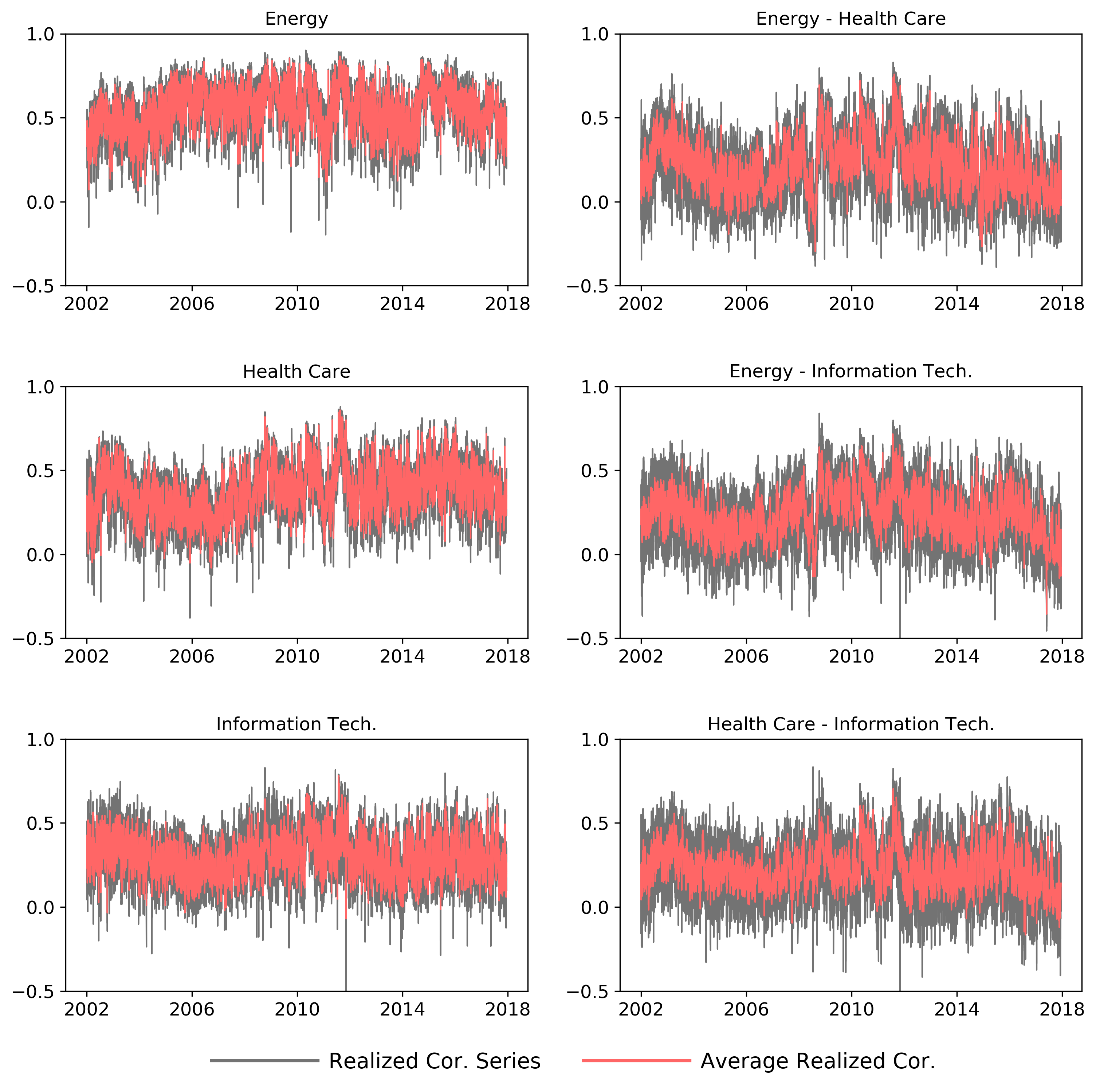
Figure 1: Daily realized correlations for the nine returns series over the full sample period. Left subplots present intra-sector correlations (gray lines) and their average (red line) for each sector. Right subplots present inter-sector correlations (gray lines) and their average (red line) for each pair of sectors.

4.3 Transformed Realized Correlations are Approximately Gaussian

The logarithmic realized variance of stock returns is approximately Gaussian distributed, as demonstrated in Andersen et al., 2001a . This help to justify the Gaussian specification for the errors, $v_{t}$, in the measurement equation for the logarithm of realized variance measures, $\log x_{t}$. Interestingly, we find that components of the matrix logarithmically transformed realized correlation matrices are also approximately Gaussian distributed. This complementary result helps to justify the Gaussian specification adopted for the errors, $\tilde{v}_{t}$ and $\check{v}_{t}$, in the measurement equations for $y_{t}$ and $\check{y}_{t}$, respectively.

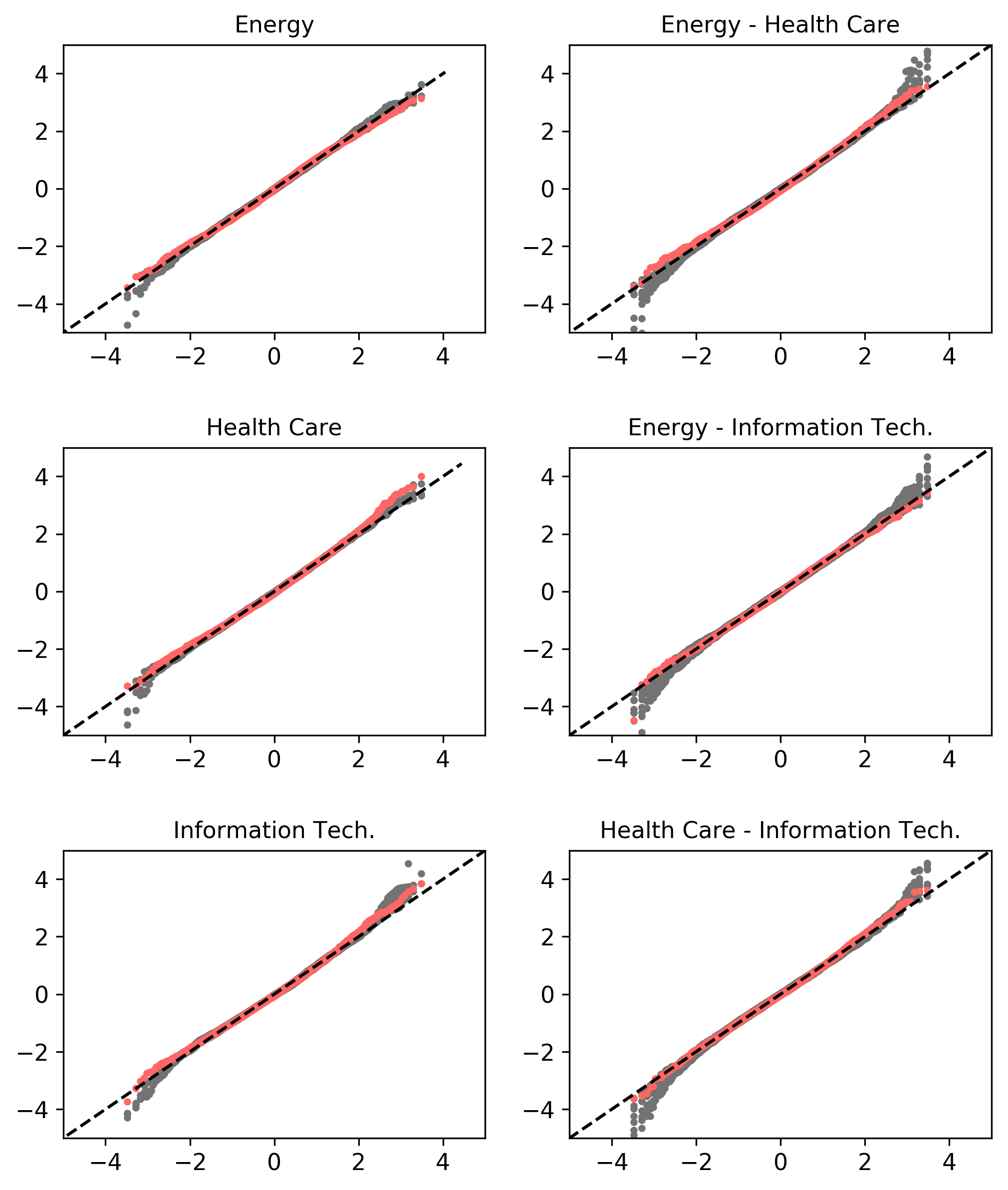
Figure 2: Q-Q plots for the components of parametrized realized correlation matrices, $y_{t}$. Within each panel, black dots are related to the multiple components of the transformed realized correlation matrix, which positions correspond to a given block. Within each panel, red dots are related to the single component of the transformed realized block correlation matrix (for which all realized correlations within each block are replaced by their average value), which corresponds to a given block. The Q-Q plots for all considered components are constructed using daily realized correlations for the period since January 2nd, 2002, until December 29th, 2017 (3975 trading days).

Figure 2 presents Q-Q plots for the empirical distribution of the transformed realized correlations against the normal distribution. For each element of $y_{t}$, the vector of logarithmic transformed correlations, we have 3975 daily observations. The quantiles of their empirical distributions are plotted against the corresponding quantiles of the normal distribution. The left panels of Figure 2 are Q-Q plots for the series in the three diagonal blocks of $Y_{t}$, which have three series in each panel. Similarly, the right panels are for the three off-diagonal blocks of $Y_{t}$, which have six series in each panel. The red dots within each panel represent the Q-Q plots for the corresponding elements of $\check{y}_{t}$, that are the daily averages within each block. The elements of $\check{y}_{t}$ are the relevant series in the model, where we impose a block correlation structure, see Section 2.4.

The Q-Q plots in Figure 2 show that the components of $y_{t}$ have an empirical distribution that is well approximated by the Gaussian distribution, albeit with some deviations in the tail regions where the discrepancy is most pronounced for the between-sector blocks, as can be seen in the right panels of Figure 2. The red dots that represent Q-Q plots for the block averages, which define the elements of $\check{y}_{t}$, show that their empirical distributions are very well approximated by the Gaussian distribution. This is not entirely unexpected since the elements of $\check{y}_{t}$ are defined as averages over elements of $y_{t}$.

4.4 Empirical Analysis of the Multivariate Realized GARCH model

We estimate the model using six different specifications for the correlation matrix. The six specifications arise from the combinations of three structures for $C_{t}$: equicorrelation, block correlation, and a “free” correlation structure, and the two ways in which we model the correlations: static and dynamic. The simplest model in our comparison is the static equicorrelation model which has a single correlation coefficient. This correlation coefficient is common for all correlations in $C_{t}$, and is constant over time. The most general specification is the dynamic correlation matrix with 36 unrestricted correlations (aside from the requirement that $C_{t}$ be positive definite). In this model, $\varrho_{t}$ is a 36-dimensional vector, whereas $\varrho_{t}$ is univariate in the dynamic equicorrelation model, and $\varrho_{t}$ has dimension six in the dynamic block correlation model.

All model specifications use the same Realized GARCH structure to model each of the nine conditional variances, $h_{1,t},\ldots,h_{9,t}$. So the six specifications only differ in terms of the way the correlation matrix is modeled. The dynamic equicorrelation model use one latent variable to model the time variation in the correlation matrix, the dynamic block correlation model employs six latent variables for this purpose, whereas the dynamic “free” correlation model has 36 latent variables. Here, $d=36=10\times 9/2$ is the number of distinct correlation coefficients in $C_{t}$, when the correlation matrix is not subject to any restrictions beyond being positive definite.

		Static correlation			Dynamic correlation
Parameter		Equi	Block	Free	Equi	Block	Free
	$\mu$	[0.026, 0.142]	[0.023, 0.140]	[0.022, 0.138]	[0.023, 0.135]	[0.014, 0.139]	[0.012, 0.148]
Variance parameters	$\omega$	[-0.008, 0.229]	[-0.011, 0.205]	[-0.009, 0.201]	[-0.006, 0.209]	[-0.002, 0.188]	[0.000, 0.174]
	$\beta$	[0.483, 0.728]	[0.490, 0.728]	[0.488, 0.728]	[0.501, 0.723]	[0.507, 0.737]	[0.544, 0.763]
	$\Gamma$	[0.232, 0.428]	[0.231, 0.426]	[0.231, 0.426]	[0.241, 0.430]	[0.227, 0.418]	[0.201, 0.382]
	$\tau_{1}$	[-0.031, 0.000]	[-0.031, 0.000]	[-0.031, -0.000]	[-0.032, 0.001]	[-0.031, 0.003]	[-0.029, 0.004]
	$\tau_{2}$	[-0.007, 0.031]	[-0.007, 0.029]	[-0.007, 0.030]	[-0.007, 0.030]	[-0.007, 0.027]	[-0.007, 0.025]
	$\xi$	[-0.417, -0.002]	[-0.400, 0.009]	[-0.391, 0.003]	[-0.388, -0.004]	[-0.391, -0.015]	[-0.384, -0.028]
	$\delta_{1}$	[-0.070, 0.005]	[-0.068, 0.005]	[-0.069, 0.005]	[-0.066, 0.012]	[-0.064, 0.012]	[-0.067, 0.013]
	$\delta_{2}$	[0.015, 0.090]	[0.015, 0.088]	[0.015, 0.088]	[0.015, 0.091]	[0.014, 0.091]	[0.014, 0.084]
	$\sigma^{2}_{v}$	[0.153, 0.298]	[0.154, 0.298]	[0.154, 0.298]	[0.154, 0.297]	[0.155, 0.297]	[0.157, 0.299]
	$\pi$	[0.910, 0.975]	[0.912, 0.973]	[0.912, 0.973]	[0.920, 0.978]	[0.920, 0.977]	[0.926, 0.976]
Correlation parameters	$\bar{\rho}$	0.322	[0.227, 0.705]	[0.198, 0.710]
	$\tilde{\omega}$				-0.009	[-0.008, 0.048]	[-0.016, 0.035]
	$\tilde{\beta}$				0.667	[0.713, 0.800]	[0.828, 0.958]
	$\tilde{\Gamma}$				0.405	[0.140, 0.320]	[0.021, 0.205]
	$\tilde{\xi}$				0.042	[-0.099, 0.076]	[-0.112, 0.140]
	$\tilde{\Phi}$				0.720	[0.640, 1.411]	[0.384, 1.663]
	$\sigma^{2}_{\tilde{v}}$				0.001	[0.002, 0.009]	[0.010, 0.020]
	$\tilde{\pi}$				0.959	[0.927, 0.982]	[0.966, 0.992]
	$\mathcal{L}$	-63851.475	-61912.446	-61828.382	-63466.324	-61419.596	-61345.306

Table 3: Parameter estimates for the six model specifications. The first three columns with estimates are for the static correlation models, and the last three columns are for the dynamic correlation models. Within each specification, we report the range of estimates for each parameter-type, unless the specification only has a single parameter of this type, in which case we report the point estimate. Persistence of volatilities and correlations are summarized by $\pi=\beta+\gamma$ and $\bar{\pi}=\bar{\beta}+\bar{\gamma}\bar{\Phi}$, respectively. The partial log-likelihood (for returns) is reported in the last row for each of the specifications.

Parameter estimates for each of the six different specifications are reported in Table 3. The estimates are based on our full sample that spans the period from January 3, 2002, to December 29, 2017. Each column in Table 3 corresponds to one of the six specifications. The first three columns are the three static models, and the last three columns are the three dynamic models. Rather than reporting a very large number of point estimates, we report the range of estimates for each “type” of parameter. For instance, each of nine the GARCH equations, for $h_{1,t},\ldots,h_{9,t}$, have an intercept, $\omega$, and the smallest and largest estimates of $\omega$ in the equicorrelation model with a constant correlation, was $-0.008$ and $0.229$, respectively.

In the upper panel, we present the point estimates for the part of the model that relates to the conditional variances, and these point estimates are in line with point estimates reported in the existing literature on GARCH models and Realized GARCH models. A simple measure of persistence of the conditional variance is given by $\pi=\beta+\gamma$, and these estimates are all close to unity, which is to be expected since volatility is known to be highly persistent.

The lower panel of Table 3 presents the point estimates for the parameters that characterize the correlation structure. For all the dynamic specifications we also observe a high level of persistence for the conditional correlations, as it is the case for the conditional variances.

It is not meaningful to compare the total log-likelihood of the different specifications, because they involve measurement equations with different dimensions. While all the specifications model the vector of returns, they differ in terms of the realized measures that are being modeled. For instance, the static specifications do not model any of the realized correlations. However, we can compare the models in terms of their partial log-likelihood for returns, $\ell_{r,t}(\theta)$, which we will refer to as the return log-likelihood. The return log-likelihood is an interesting metric because the practical objective is typically to obtain a good model for the conditional distribution of returns. We can compute likelihood ratio statistics based on the partial log-likelihoods alone, and these will reflect which of the models has the best description of the conditional distribution of returns, in the Kullback-Leibler sense. But we cannot compare these likelihood-ratio statistics to standard $\chi^{2}$-based critical values, because the return log-likelihood is only one of two parts of the total log-likelihood. The other term is the log-likelihood for realized measures of volatilities and correlations, and the degrees of freedom differ across model specifications.

From the return log-likelihood, it is evident that the equicorrelation structure is inferior to the more flexible structures. The return log-likelihood is about 2000 larger with block and free structures than the equicorrelation structure, which is a very substantial empirical improvement. Specifications with a dynamic structure rather than static also have far larger values of the return log-likelihood. For both the block correlation and the free correlation structures, the dynamic specifications have a return log-likelihood that are about 415 larger than those of the static specifications. The dynamic model with an unrestricted correlation structure increases the partial log-likelihood function by about 74 units, relative to the dynamic block correlation model.

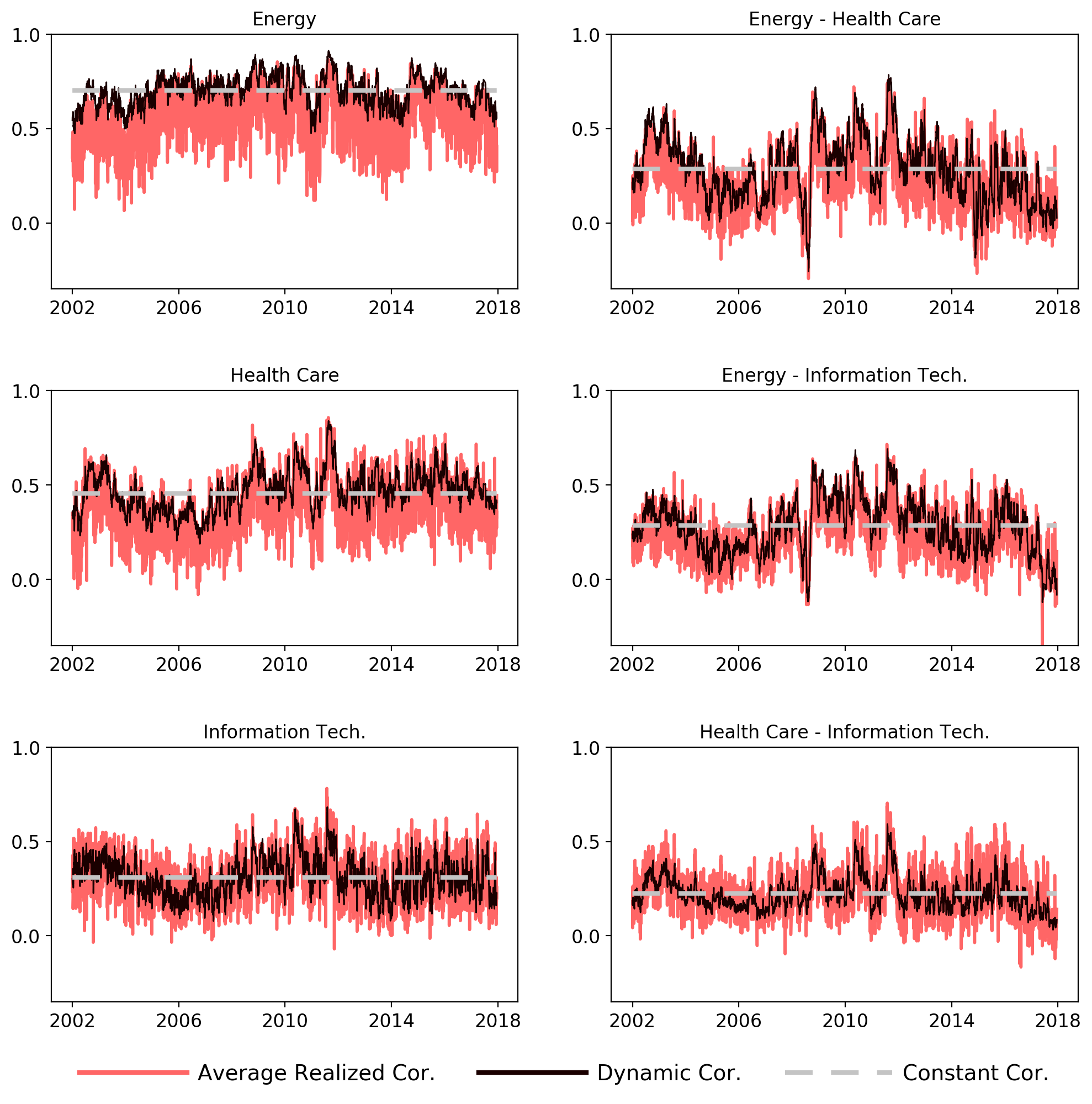
Figure 3: Within-sector and between-sector correlations. The left subplots present the model-based correlations for each of the three sectors (black lines) and the corresponding daily averages of realized correlations (red lines). The estimates from the constant correlation model are indicated by white dashed lines. The right panels present the correlations across sectors.

To illustrate the correlation structure that one of the estimated models produces, we present the six conditional correlation series, produced by the estimated block correlation model, in Figure 3. The figure also displays the average of the corresponding daily realized correlations. The left panels present the model-based correlation (black line) within each of the three sectors, and the corresponding daily average of the realized correlations is represented with the red line. The right panels present the results for between-sector correlations. The analogous figure for the models with an equicorrelation structure can be seen in the appendix.

According to the log-likelihood functions for returns over the full sample period, there are substantial gains from moving beyond the equicorrelation model and adopting a dynamic model for the correlations. In the next section, we evaluate the extent to which these improvements carry over to improved empirical fit in an out-of-sample comparison.

4.5 Out-of-Sample Model Comparisons

In this section, we compare the six different specifications in terms of their out-of-sample performance. To this end, we split the sample period into an in-sample period and an out-of-sample period. The in-sample period lasts from January 2nd, 2002, to December 31st, 2013, and includes 2993 trading days. The out-of-sample period spans the period from January 2nd, 2014, to December 29th, 2017, and has 982 trading days. We employ the so-called fixed scheme, where each model is estimated once using the data from the in-sample period. Then the estimated models are evaluated and compared out-of-sample using a range of criteria.

We first compare the models in terms of their partial log-likelihood for returns, then we turn to the other criteria – a minimum variance portfolio selection.

4.5.1 Analysis of Log-Likelihood for Returns

Multivariate GARCH models seek to describe the conditional distribution of the vector of returns. This objective is defined by the log-likelihood function for returns that is used in the estimation. A natural starting point for comparing the different specifications is, therefore, a comparison of their return log-likelihoods, which measures how well the estimated model can explain the distribution of the return vector. So, in this subsection, we evaluate and compare the specifications in terms of their average value of $\ell_{r,t}(\hat{\theta})$ (both in-sample and out-of-sample), where the parameter vector $\hat{\theta}$ is estimated with the in-sample data. This type of model evaluation is equivalent to one-day-ahead density forecasting of the return vector with the mean predictive log-likelihood as a gain function, see Amisano and Giacomini, (2007), Geweke and Amisano, (2010), and references therein.

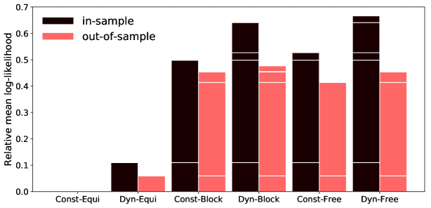
Figure 4: Average in-sample (black) and out-of-sample (red) return log-likelihoods, measured relative to the static equicorrelation specification. The horizontal white lines depict the performance of competing models. The in-sample period is January 2nd, 2002, to December 31st, 2013, (2993 trading days) and the out-of-sample period is January 2nd, 2014 to December 29th, 2017 (982 trading days).

We compute the average in-sample and average out-of-sample return log-likelihoods, for each of the six specifications. Figure 4 is a bar chart with the relative return log-likelihood of each specification with respect to the static equicorrelation structure. So a positive value (which is observed for all other specifications) corresponds to better performance than the static equicorrelation model. Both the in-sample and out-of-sample log-likelihood increases by adopting a more flexible correlation structure. The in-sample log-likelihood increases with the complexity of the model, as it to be expected. So the simplest model, the static equicorrelation model, has the smallest in-sample log-likelihood, whereas the “free” dynamic model with 36 latent variables to describe the correlation structure has the largest in-sample log-likelihood. A good in-sample fit need not translate into good out-of-sample fit. Nevertheless, we do find that the two specifications with the lowest in-sample fit (static and dynamic equicorrelation) also have the lowest out-of-sample fit. The two equicorrelation models have substantially lower performance than all of the block and free-correlation specifications. Among the block correlation models and the free correlation models it is evident that the dynamic models do better than the static models. This is not only true in-sample, but also out-of-sample. Interestingly, it is the dynamic block correlation model that has the highest out-of-sample fit. So, the better in-sample fit of the dynamic-free specification indeed does not translate into a better out-of-sample fit. In fact, it is barely better than the static block correlation model. This is an indication that the most flexible specification with 36 latent variables to describe the correlation structure is overfitting the in-sample data.

Table 4 adds further information about the comparison in terms of the return log-likelihoods, and the statistical significance of the relative performance. We report the average per-period improvement of the return log-likelihood relative to the simplest specification with the static equicorrelation. We evaluate the statistical significance of the relative return log-likelihoods using the model confidence set (MCS) by Hansen et al., (2011). We seek the specification with the largest expected out-of-sample partial log-likelihood, and the MCS is the subset of models that contains the best with a given level of confidence, after the original set of models has been trimmed by eliminating significantly inferior models in a sequential testing procedure. The MCS $p$-values are reported in parentheses and a small $p$-value is evidence that the model is significantly outperformed by other models in the comparison. The specifications in the 95% MCS are identified with bold font.

The relative average return log-likelihoods are reported for the in-sample period as a point of reference. Over the out-of-sample period, we find that the dynamic block correlation model has the best overall out-of-sample performance, but the MCS also includes the dynamic-free and the static-block specifications. The latter is included in the MCS because it performed particularly well in 2015. We also compare the specifications for each of calendar years in the out-of-sample period. For three of the four years, the dynamic block correlation specification has the best out-of-sample performance.

	Static correlation			Dynamic correlation
Period	Equi	Block	Free	Equi	Block	Free
In-sample	0.000	0.499	0.527	0.110	0.641	0.666
[2002-2013]
Out-of-sample	0.000	0.453	0.414	0.060	0.477	0.455
[2014-2017]	(0.00)	(0.51)	(0.00)	(0.00)	(1.00)	(0.45)
2014	0.000	0.369	0.360	0.029	0.440	0.420
	(0.00)	(0.09)	(0.09)	(0.01)	(1.00)	(0.52)
2015	0.000	0.663	0.570	-0.051	0.550	0.561
	(0.00)	(1.00)	(0.00)	(0.00)	(0.00)	(0.19)
2016	0.000	0.366	0.346	0.070	0.371	0.336
	(0.01)	(0.95)	(0.63)	(0.06)	(1.00)	(0.63)
2017	0.000	0.412	0.377	0.201	0.551	0.507
	(0.00)	(0.24)	(0.09)	(0.02)	(1.00)	(0.24)

Table 4: Average out-of-sample partial log-likelihood relative to the constant equicorrelation model. Model confidence $p$-values are given in parentheses, and those significant at the 5% level are shaded gray. The comparisons are done for the entire out-of-sample period, 2014-2017, and for each of the years separately.

4.5.2 Global Minimum-Variance Portfolio

In this section, we evaluate and compare the ability of the estimated models to produce a low-variance portfolio out-of-sample. At time $t-1$, we seek portfolio weights that minimize the variance of the portfolio return over the next period. Hence, for each of the specifications, we deduce the implied global minimum-variance (GMV) portfolio. The optimal portfolio weights solve

$$\begin{array}[]{ccc}\min_{\omega_{t}\in\mathbb{R}^{p}}\omega_{t}^{\prime}H_{(j),t}\omega_{t},&&\text{s.t. }\omega_{t}^{\prime}\iota=1,\end{array}$$

where $H_{(j),t}$ is the model-based conditional variance of the return vector, $r_{t}\in\mathbb{R}^{p}$, $j=1,\ldots,6$, and $\iota=(1,\ldots,1)^{\prime}$ is a $p$-dimensional vector of ones. In the absence of leverage constraints (such as no-shortening constraints), the well-know solution to this portfolio problem is:

$$\omega_{(j),t}^{*}=\frac{H_{(j),t}^{-1}\iota}{\iota^{\prime}H_{(j),t}^{-1}\iota},$$

and the resulting portfolio returns are given by

$$R_{(j),t}^{\mathrm{mv}}=\omega_{(j),t}^{*\prime}r_{t}.$$

Because the different specifications produce different covariance matrices, $H_{(j),t}$, $j=1,\ldots,$6, the resulting portfolio returns will differ, and may therefore have different variances and distributions. For illustrative purposes, we add the simple equal-weighted portfolio to the comparison. The returns of the equal-weighted portfolio are simply given by

$$R_{\mathrm{ew},t}=\frac{1}{p}\iota^{\prime}r_{t},$$

so that each asset is weighted by $1/p$, where $p=9$ in this application.

We will compare the variance of the seven portfolios, to evaluate whether the different specifications produce substantially different portfolio variances. We report the in-sample and out-of-sample variances of the seven portfolios in the upper panel of Table 5. The first observation we make is that the equal-weighted portfolio has substantially larger variance than any of the model-based portfolios. This is not unexpected because the equal-weighted portfolio does not use any information about the covariance structure. On the other hand, the fact that the model-based portfolios can reduce the variance by a factor of two is evidence that all of the multivariate realized GARCH specifications produce sensible and valuable forecasts of the conditional covariance matrix, $H_{t}$.

Among the six model-based portfolios it is the most flexible specification (dynamic-free) that has the smallest out-of-sample variance, in the (full) out-of-sample period. The portfolio based on the dynamic-block specification comes in as a close second, however, all but the simplest static equicorrelation specification are found in the model confidence set. We also present results for each of the years in the out-of-sample period, and while there is some variation from year to year, the dynamic-free portfolio end up in the MCS every year.

		Equal	Static correlation			Dynamic correlation
Period		weights	Equi	Block	Free	Equi	Block	Free
Squared returns	In-sample	2.149	1.117	1.091	1.077	1.063	0.990	0.991
	[2002-2013]
	Out-of-sample	0.952	0.506	0.475	0.466	0.499	0.471	0.464
	[2014-2017]	(0.00)	(0.01)	(0.21)	(0.93)	(0.14)	(0.66)	(1.00)
	2014	0.657	0.588	0.553	0.546	0.577	0.542	0.525
		(0.02)	(0.02)	(0.25)	(0.25)	(0.10)	(0.25)	(1.00)
	2015	1.393	0.695	0.580	0.596	0.712	0.606	0.629
		(0.00)	(0.01)	(1.00)	(0.27)	(0.01)	(0.27)	(0.15)
	2016	1.385	0.471	0.498	0.465	0.491	0.525	0.496
		(0.00)	(0.86)	(0.02)	(1.00)	(0.83)	(0.02)	(0.86)
	2017	0.324	0.251	0.254	0.240	0.194	0.191	0.188
		(0.00)	(0.00)	(0.00)	(0.01)	(0.76)	(0.76)	(1.00)
Abs. returns (annual)	In-sample	0.158	0.113	0.111	0.110	0.111	0.107	0.106
	[2002-2013]
	Out-of-sample	0.114	0.085	0.082	0.081	0.082	0.080	0.079
	[2014-2017]	(0.00)	(0.00)	(0.11)	(0.15)	(0.02)	(0.54)	(1.00)
	2014	0.096	0.095	0.090	0.089	0.093	0.087	0.087
		(0.01)	(0.00)	(0.18)	(0.18)	(0.01)	(0.57)	(1.00)
	2015	0.145	0.099	0.092	0.094	0.100	0.094	0.097
		(0.00)	(0.00)	(1.00)	(0.12)	(0.00)	(0.35)	(0.06)
	2016	0.141	0.081	0.083	0.080	0.081	0.082	0.078
		(0.00)	(0.40)	(0.01)	(0.41)	(0.40)	(0.04)	(1.00)
	2017	0.071	0.061	0.062	0.060	0.054	0.053	0.053
		(0.00)	(0.00)	(0.00)	(0.00)	(0.70)	(0.80)	(1.00)

Table 5: The average of squared returns (top panel) and absolute returns (bottom panel) for the equal-weighted portfolio and the six global minimum variance portfolios. The in-sample period is January 2nd, 2002, to December 31st, 2013, (3021 trading days) and the out-of-sample period is January 2nd, 2014, to December 29th, 2017, (989 trading days). We also report results for each of the calendar years in the out-of-sample period. Numbers in parentheses are MCS $p$-values and bold numbers indicate specifications that are in the $95\%$ MCS.

A variance comparison is based on squared returns, which is sensitive to outliers. We, therefore, supplement the comparison with a comparison of absolute portfolio returns. These results are presented in the lower panel of Table 5, where we present the mean of absolute daily returns, measured in annualized units. These results, including the model confidence sets, are almost identical to the results obtained with squared returns.

This comparison is further evidence that dynamic and flexible correlation modeling leads to significant improvements out-of-sample. Relative to the simplest model, the static equicorrelation specification, we observe a variance reduction of about 50 basis points in annual volatility. In practice, one would also want to factor in portfolio turnover, because transaction costs may offset the gain from the variance reduction. This would entails a model comparison based on a different criterion. We leave this for future research.

5 Conclusion and Discussion

In this paper, we have introduced a novel framework for multivariate GARCH modeling. The framework is based on a vector parametrization of correlation matrices, where the $p\times p$ correlation matrix, $C_{t}$, is represented by the $d=p(p-1)/2$ dimensional vector, $\varrho_{t}=g(C_{t})$. Our methodological contribution is to propose the dynamic correlation matrix using a model for $\varrho_{t}$. In its most general form, the parametrization, $\varrho_{t}=g(C_{t})$, does not impose any restrictions on $C_{t}$, aside from ensuring that $C_{t}$ is positive definite. However, in many situations, it will be desirable to impose additional structure on $C_{t}$. A key advantage of the proposed model, is that the factor model for $\varrho_{t}$ makes it straightforward to reduce the number of free parameters and latent variables. We found that a block correlation structure implies a simple linear factor model, $\varrho_{t}=A\zeta_{t}$, where $A$ is a known matrix. The linear structure is not specific to model with block correlation matrices. Other choices for $A$ could be entertained, and different $A$-matrices will induce different (parsimonious) structures on $C_{t}$. It is also possible to explore data-dependent choices for $A$, as well as non-linear factor structures. We leave these generalizations for future research.

The Multivariate Realized GARCH model utilizes realized measures of volatilities and correlations. We applied the model to nine assets from three different sectors. We estimated different specifications using combination of three correlation structures (equicorrelation, block correlation, and unrestricted) with either static or dynamic correlations. The empirical results favor dynamic specifications for $C_{t}$ and strongly prefer the block structure or the unrestricted structure over the equicorrelation structure. It is encouraging that the dynamic block correlation specification performs well in-sample and out-of-sample, because this model can be easily scaled to higher dimensions.

Appendix A Estimation Procedure in Details

In this appendix, we provide a detailed description of the estimation procedure for the Multivariate Realized GARCH model, when $\varrho_{t}=A\zeta_{t}$. In the unrestricted case ($A=I$), we have $\varrho_{t}=\zeta_{t}$. The data consists of the $p$-dimensional return vector, $r_{t}$, for $t=1,...,T$, and the corresponding transformed realized measures. The realized measures consist of the $p$-dimensional vector of realized variances, $x_{t}$, and the $k$-dimensional vector of transformed correlations, $\check{y}_{t}=(A^{\prime}A)^{-1}A^{\prime}y_{t}$, where the “free” specification $(A=I)$ has $\check{y}_{t}=y_{t}$ and $k=d=p(p-1)/2$.

The log-likelihood is evaluated using the following steps:

1. Initialize all parameters, except $\Sigma$, and let these be represented by $\theta$. Also, initialize starting values for the conditional variances and the transformed conditional correlations, $h_{1}$ and $\zeta_{1}$. We will maximize the log-likelihood with respect to $(\theta,h_{1},\zeta_{1})$. An alternative approach is to fix values for $h_{1}$ and $\zeta_{1}$. For example, using an appropriate sample average.

2. Compute $h_{t}(\theta)$ and $\zeta_{t}(\theta)$ using the GARCH equations, and map the latter to $\varrho_{t}=A\zeta_{t}$ and then to $C_{t}(\theta)$, for $t=1,...,T$. The mapping from $\varrho_{t}$ to $C_{t}$ can be done with the algorithm provided in Archakov and Hansen, 2020b (, corollary 1).

3. Compute the standardized returns, $z_{t}(\theta)$, and the measurement errors, $u_{t}(\theta)$, for $t=1,...,T$.

4. Compute $\hat{\Sigma}(\theta)=T^{-1}\sum_{t}u_{t}(\theta)u_{t}(\theta)^{\prime}$ and evaluate the log-likelihood using (11).

The model can now be estimated by maximizing (11) with respect to $\theta$, $h_{1}$, and $\zeta_{1}$, by repeating steps 2, 3 and 4 every time $(\theta,h_{1},\zeta_{1})$ has been updated.

Appendix B Additional Empirical Results

In Figure B.1, we plot the 36 realized correlation series (grey lines) as well as the average realized correlation (red line). While it is not possible to identify the paths of the individual correlation series in Figure B.1, it does reveal a great deal of dispersion across the individual correlations relative to the average correlation series.

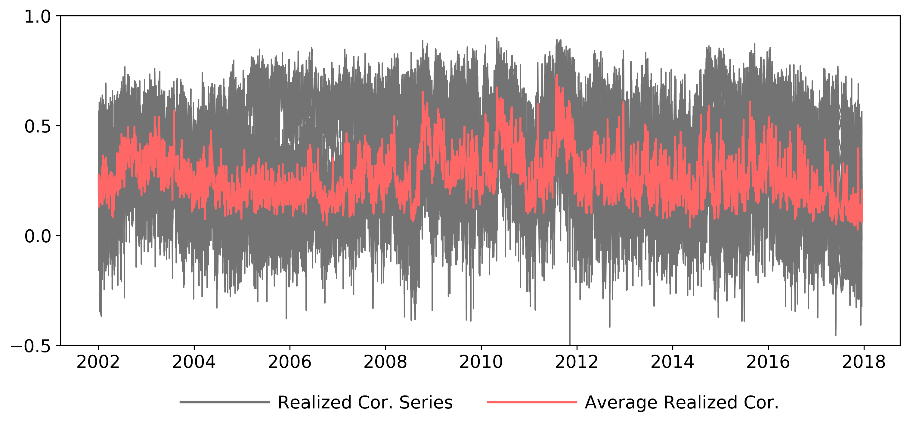
Figure B.1: Daily realized correlations for the full sample period. The realized correlations for the 36 correlation series (grey lines) are computed from the multivariate Realized Kernel estimator. The red line is the time series with the daily average correlation.

The estimated time series for the equicorrelation model is presented in Figure B.2. The red line is the average realized correlation, and the black line is the time series of $\rho_{t}$, as produced by the estimated dynamic equicorrelation model. The estimate of the constant equicorrelation model is illustrated with the dashed line.

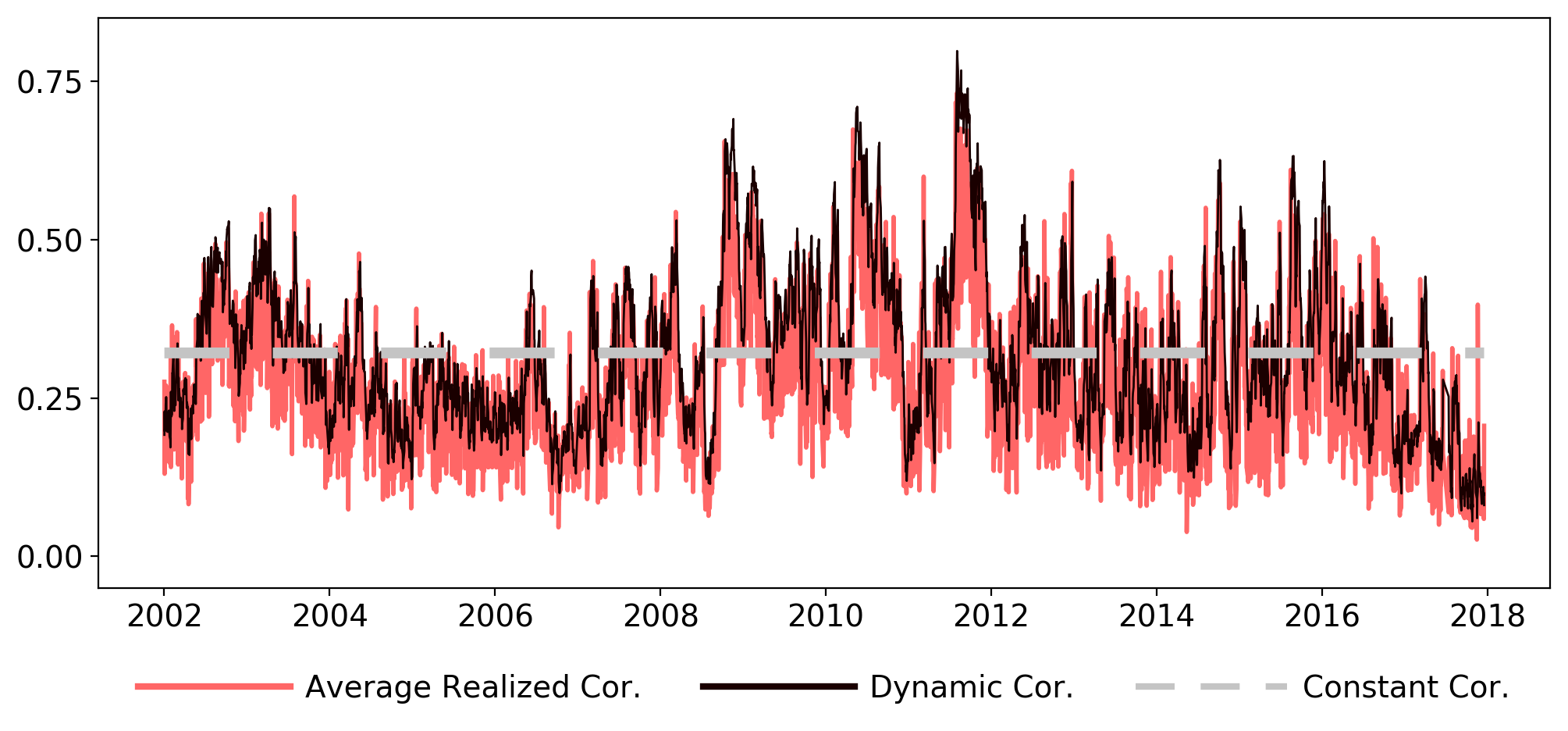
Figure B.2: The common correlation coefficient deduced from the estimated equicorrelation model (black line) and the daily average of the 36 realized correlations (red line). The gray dashed line represents the estimate of the common correlation coefficient produced by the constant equicorrelation structure.

References

- Aielli, (2013) Aielli, G. P. (2013). Dynamic conditional correlation: on properties and estimation. Journal of Business and Economic Statistics, 31:282–299.
- Amisano and Giacomini, (2007) Amisano, G. and Giacomini, R. (2007). Comparing Density Forecasts via Weighted Likelihood Ratio Tests. Journal of Business & Economic Statistics, 25:177–190.
- Andersen and Bollerslev, (1998) Andersen, T. G. and Bollerslev, T. (1998). Answering the skeptics: Yes, standard volatility models do provide accurate forecasts. 39(4):885–905.
- (4) Andersen, T. G., Bollerslev, T., Diebold, F. X., and Ebens, H. (2001a). The distribution of realized stock return volatility. Journal of Financial Economics, 61:43–76.
- (5) Andersen, T. G., Bollerslev, T., Diebold, F. X., and Labys, P. (2001b). The distribution of realized exchange rate volatility. Journal of the American Statistical Association, 96:42–55.
- Andersen et al., (2003) Andersen, T. G., Bollerslev, T., Diebold, F. X., and Labys, P. (2003). Modeling and forecasting realized volatility. Econometrica, 71:579–625.
- (7) Archakov, I. and Hansen, P. R. (2020a). A canonical representation of block matrices with applications to covariance and correlation matrices. https://sites.google.com/site/peterreinhardhansen/.
- (8) Archakov, I. and Hansen, P. R. (2020b). A new parametrization of correlation matrices. Econometrica, forthcoming.
- Asai and So, (2015) Asai, M. and So, M. (2015). Long memory and asymmetry for matrix-exponential dynamic correlation processes. Journal of Time Series Econometrics, 7:69–74.
- Barndorff-Nielsen et al., (2009) Barndorff-Nielsen, O. E., Hansen, P. R., Lunde, A., and Shephard, N. (2009). Realized kernels in practice: trades and quotes. Econometrics Journal, 12:C1–C32.
- Barndorff-Nielsen et al., (2011) Barndorff-Nielsen, O. E., Hansen, P. R., Lunde, A., and Shephard, N. (2011). Multivariate realised kernels: consistent positive semi-definite estimators of the covariation of equity prices with noise and non-synchronous trading. Jounal of Econometrics, 162:149–169.
- (12) Barndorff-Nielsen, O. E. and Shephard, N. (2002a). Estimating quadratic variation using realized variance. Journal of Applied Econometrics, 17(5):457–477.
- (13) Barndorff-Nielsen, O. E. and Shephard, N. (2002b). How accurate is the asymptotic approximation to the distribution of realised variance. Economics Series Working Papers 2001-W16, University of Oxford, Department of Economics.
- (14) Barndorff-Nielsen, O. E. and Shephard, N. (2004a). Econometric analysis of realized covariation: High frequency based covariance, regression, and correlation in financial economics. Econometrica, 72:885–925.
- (15) Barndorff-Nielsen, O. E. and Shephard, N. (2004b). Econometric Analysis of Realized Covariation: High Frequency Based Covariance, Regression, and Correlation in Financial Economics. Econometrica, 72(3):885–925.
- Bauer and Vorkink, (2011) Bauer, G. H. and Vorkink, K. (2011). Forecasting multivariate realized stock market volatility. Journal of Econometrics, 160:93–101.
- Bauwens et al., (2012) Bauwens, L., Storti, G., and Violante, F. (2012). Dynamic conditional correlation models for realized covariance matrices. Working Paper, (2012060).
- Black, (1976) Black, F. (1976). Studies of Stock Price Volatility Changes. Proceedings of the 1976 Meetings of the American Statistical Association, Business and Economic Statistics Section.
- Bollerslev, (1990) Bollerslev, T. (1990). Modelling the coherence in short-run nominal exchange rates: A multivariate generalized ARCH model. The Review of Economics and Statistics, 72:498–505.
- Chiriac and Voev, (2011) Chiriac, R. and Voev, V. (2011). Modelling and forecasting multivariate realized volatility. Journal of Applied Econometrics, 26:922–947.
- Chiu et al., (1996) Chiu, T., Leonard, T., and Tsui, K.-W. (1996). The matrix-logarithmic covariance model. Journal of the American Statistical Association, 91:198–210.
- Christie, (1982) Christie, A. A. (1982). The stochastic behavior of common stock variances : Value, leverage and interest rate effects. Journal of Financial Economics, 10:407–432.
- Dumitrescu and Hansen, (2017) Dumitrescu, E. and Hansen, P. (2017). Forecasting exchange rate volatility: Multivariate realized GARCH framework. Working Paper.
- Engle and Kelly, (2012) Engle, R. and Kelly, B. (2012). Dynamic Equicorrelation. Journal of Business & Economic Statistics, 30(2):212–228.
- Engle, (1982) Engle, R. F. (1982). Autoregressive conditional heteroskedasticity with estimates of the variance of U.K. inflation. Econometrica, 45:987–1007.
- (26) Engle, R. F. (2002a). Dynamic Conditional Correlation: A Simple Class of Multivariate Generalized Autoregressive Conditional Heteroskedasticity Models. Journal of Business & Economic Statistics, 20(3):339–350.
- (27) Engle, R. F. (2002b). New frontiers for arch models. Journal of Applied Econometrics, 17(5):425–446.
- Engle and Gallo, (2006) Engle, R. F. and Gallo, G. (2006). A multiple indicators model for volatility using intra-daily data. Journal of Econometrics, 131:3–27.
- Engle et al., (2019) Engle, R. F., Ledoit, O., and Wolf, M. (2019). Large dynamic covariance matrices. Journal of Business and Economic Statistics, 37:363–375.
- Engle and Ng, (1993) Engle, R. F. and Ng, V. K. (1993). Measuring and Testing the Impact of News on Volatility. Journal of Finance, 48:1749–78.
- Engle and Sheppard, (2001) Engle, R. F. and Sheppard, K. (2001). Theoretical and Empirical properties of Dynamic Conditional Correlation Multivariate GARCH. NBER Working Papers 8554, National Bureau of Economic Research, Inc.
- Geweke and Amisano, (2010) Geweke, J. and Amisano, G. (2010). Comparing and evaluating Bayesian predictive distributions of asset returns. International Journal of Forecasting, 26(2):216–230.
- Golosnoy et al., (2012) Golosnoy, V., Gribisch, B., and Liesenfeld, R. (2012). The conditional autoregressive Wishart model for multivariate stock market volatility. Journal of Econometrics, 167(1):211–223.
- Gorgi et al., (2019) Gorgi, P., Hansen, P. R., Janus, P., and Koopman, S. J. (2019). Realized Wishart-GARCH: A score-driven multi-asset volatility model. Journal of Financial Econometrics, 17:1–32.
- Hansen and Huang, (2016) Hansen, P. R. and Huang, Z. (2016). Exponential GARCH modeling with realized measures of volatility. Journal of Business & Economic Statistics, 34:269–287.
- Hansen et al., (2012) Hansen, P. R., Huang, Z., and Shek, H. (2012). Realized GARCH: A joint model of returns and realized measures of volatility. Journal of Applied Econometrics, 27:877–906.
- Hansen and Lunde, (2011) Hansen, P. R. and Lunde, A. (2011). Forecasting Volatility Using High-Frequency Data. The Oxford Handbook of Economic Forecasting.
- Hansen et al., (2011) Hansen, P. R., Lunde, A., and Nason, J. M. (2011). The Model Confidence Set. Econometrica, 79(2):453–497.
- Hansen et al., (2014) Hansen, P. R., Lunde, A., and Voev, V. (2014). Realized beta GARCH: A multivariate GARCH model with realized measures of volatility. Journal of Applied Econometrics, 29:774–799.
- Ishihara et al., (2016) Ishihara, T., Omori, Y., and Asai, M. (2016). Matrix exponential stochastic volatility with cross leverage. Computational Statistics & Data Analysis, 100:331–350.
- Kawakatsu, (2006) Kawakatsu, H. (2006). Matrix exponential GARCH. Journal of Econometrics, 134:95–128.
- Liu, (2009) Liu, Q. (2009). On portfolio optimization: How and when do we benefit from high-frequency data? Journal of Applied Econometrics, 24(4):560–582.
- Lunde and Olesen, (2014) Lunde, A. and Olesen, K. V. (2014). Modeling and forecasting the volatility of energy forward returns. Working Paper.
- Noureldin et al., (2012) Noureldin, D., Shephard, N., and Sheppard, K. (2012). Multivariate high-frequency-based volatility (HEAVY) models. Journal of Applied Econometrics, 27:907–933.
- Shephard and Sheppard, (2010) Shephard, N. and Sheppard, K. (2010). Realising the future: forecasting with high-frequency-based volatility (HEAVY) models. Journal of Applied Econometrics, 25(2):197–231.
- Shephard et al., (2020) Shephard, N., Sheppard, K., and Engle, R. F. (2020). Fitting vast dimensional time-varying covariance models. Journal of Business and Economic Statistics.
- Weigand, (2014) Weigand, R. (2014). Matrix Box-Cox models for multivariate realized volatility. Working Paper.
- White, (1994) White, H. (1994). Estimation, Inference and Specification Analysis. Cambridge University Press, Cambridge.