Numerical approximation of boundary value problems for curvature flow and elastic flow
in Riemannian manifolds

Abstract

We present variational approximations of boundary value problems for curvature flow (curve shortening flow) and elastic flow (curve straightening flow) in two-dimensional Riemannian manifolds that are conformally flat. For the evolving open curves we propose natural boundary conditions that respect the appropriate gradient flow structure. Based on suitable weak formulations we introduce finite element approximations using piecewise linear elements. For some of the schemes a stability result can be shown. The derived schemes can be employed in very different contexts. For example, we apply the schemes to the Angenent metric in order to numerically compute rotationally symmetric self-shrinkers for the mean curvature flow. Furthermore, we utilise the schemes to compute geodesics that are relevant for optimal interface profiles in multi-component phase field models.

Key words. parametric finite elements, Riemannian manifolds, curvature flow, curve shortening flow, elastic flow, curve straightening flow, geodesics, elastica, Angenent metric, Angenent torus, self-shrinkers, multi-phase field interface profiles

AMS subject classifications. 65M60, 53C44, 53A30, 35K55

1 Introduction

In this paper we consider numerical approximations for gradient flows of curves evolving in Riemannian manifolds that are conformally flat. Here we allow both closed and open curves, where in the latter case appropriate boundary conditions need be considered in order to respect the required gradient flow structure.

We define the Riemannian manifold with the help of its metric tensor as follows. On a domain $H\subset\mathbb{R}^{2}$ we let the metric tensor be given by

$$[(\vec{v},\vec{w})_{g}](\vec{z})=g(\vec{z})\,\vec{v}\,.\,\vec{w}\quad\forall\ \vec{v},\vec{w}\in{\mathbb{R}}^{2}\qquad\text{ for }\vec{z}\in H\,,$$ (1.1)

where $\vec{v}\,.\,\vec{w}=\vec{v}^{T}\,\vec{w}$ is the standard Euclidean inner product, and where $g:H\to{\mathbb{R}}_{>0}$ is a smooth positive weight function. This is the setting one obtains for a two-dimensional Riemannian manifold that is conformally equivalent to the Euclidean plane. Of course, if $g$ is constant we recover the case of a Euclidean ambient space. In local coordinates the metric is precisely given by (1.1), see e.g. [46, 58, 50]. Examples of such situations are the hyperbolic plane, the hyperbolic disc and the elliptic plane. Other examples are given by two-dimensional manifolds in $\mathbb{R}^{d}$, $d\geq 3$, that can be conformally parameterised, such as spheres without pole(s), catenoids and tori. Coordinates $(x_{1},x_{2})\in H$ together with a metric $g$ as in (1.1) are called isothermal coordinates, i.e. in all situations considered in this paper we assume that we have isothermal coordinates. We refer to Section 2 and [50, 3.29 in Section 3D] for more information.

The metric tensor (1.1) induces a notion of length in $H$. In particular, the length of a vector $\vec{v}\in{\mathbb{R}}^{2}$ at the location $\vec{z}\in H$ is defined by

$$[|\vec{v}|_{g}](\vec{z})=\left([(\vec{v},\vec{v})_{g}](\vec{z})\right)^{\frac{1}{2}}=g^{\frac{1}{2}}(\vec{z})\,|\vec{v}|\,,$$ (1.2)

whereas the length of a curve $\vec{\gamma}\in C^{1}([0,1],H)$ is given by

$$L_{g}(\vec{\gamma})=\int_{0}^{1}[|\vec{\gamma}^{\prime}(\rho)|_{g}](\vec{\gamma}(\rho))\;{\rm d}\rho=\int_{0}^{1}g^{\frac{1}{2}}(\vec{\gamma}(\rho))\,|\vec{\gamma}^{\prime}(\rho)|\;{\rm d}\rho\,.$$ (1.3)

We note that $L_{g}$, which is also called geodesic length, naturally induces a distance function in $H$, with the distance between two points $\vec{z}_{0},\vec{z}_{1}\in H$ defined as

$$\operatorname{dist}_{g}(\vec{z}_{0},\vec{z}_{1})=\inf\left\{L_{g}(\vec{\gamma}):\vec{\gamma}\in C^{1}([0,1],H)\,,\ \vec{\gamma}(0)=\vec{z}_{0}\,,\ \vec{\gamma}(1)=\vec{z}_{1}\right\}.$$

It can be shown that $(H,\operatorname{dist}_{g})$ is a metric space, see [46, Section 1.4].

We will present the mathematical details of curvature flow and elastic flow in the next section, together with the derivation of suitable boundary conditions. For now we mention that curvature flow, for a family of curves $(\Gamma(t))_{t\in[0,T]}$, can be defined as the $L^{2}$–gradient flow of geodesic length, $L_{g}(\Gamma)=\int_{\Gamma}g^{\frac{1}{2}}\;{\rm d}s$, with respect to the $L^{2}$–inner product $\langle v,w\rangle=\int_{\Gamma}v\,w\,g^{\frac{1}{2}}\;{\rm d}s$. It is often called curve shortening flow. In particular, on letting the geodesic curvature $\varkappa_{g}$ be the first variation of $L_{g}(\Gamma)$, with respect to $\langle\cdot,\cdot\rangle$, then curvature flow is given by

$$\mathcal{V}_{g}=\varkappa_{g}\,,$$

where $\mathcal{V}_{g}=g^{\frac{1}{2}}\,\mathcal{V}$, and $\mathcal{V}$ is the Euclidean normal velocity of $\Gamma$ in ${\mathbb{R}}^{2}$. Moreover, the geodesic elastic energy of $\Gamma$ is defined by $W_{g}(\Gamma)=\tfrac{1}{2}\,\int_{\Gamma}(\varkappa_{g})^{2}\,g^{\frac{1}{2}}\;{\rm d}s$, and elastic flow arises as the $L^{2}$–gradient flow of $W_{g}(\Gamma)$. The elastic energy is often called bending energy of $\Gamma$, and elastic flow is also known by the name curve straightening flow. Critical points of $W_{g}(\Gamma)$ are called elastica, and a lot of interest in elastic flow is driven by the fact that stationary solutions to the flow are elastica. Moreover, elastic flow can be a viable strategy to obtain unstable geodesics, i.e. critical points of the length $L_{g}(\Gamma)$ that are unstable under curvature flow. In fact, all geodesics satisfy $\kappa_{g}=0$, and so they represent global minimisers for the bending energy.

There is a tremendous amount of work in the literature on curvature flow and elastic flow in the Euclidean plane, both from an analytical and a numerical point of view. Curvature flow in more complex ambient spaces has been treated analytically in e.g. [37, 20, 1], while numerical approximations have been considered in [21, 56, 60, 55, 6, 12], for the case of closed curves, and in [16] for the case of open curves. Using the flow along the negative gradient of the total squared geodesic curvature functional to obtain geodesics as long-time limits has been first suggested in a seminal paper by Langer and Singer, [51]. Later the same authors used Morse theory to investigate stable critical points of the functional, [52]. The curve straightening flow has been used in [53] to compute periodic geodesics, and in [48] a variant of the flow was used to study the evolution of an elastic wire in a Riemannian manifold. Short-time existence, and in certain cases long-time existence, for elastic flow for closed curves in Riemannian manifolds has been studied analytically in [24], for the case that the manifold is a sphere, and in [29, 30, 57] for the hyperbolic plane. We are not aware of existing work on boundary value problems for elastic curves in Riemannian manifolds, but note that the case of a Euclidean ambient space has been considered in e.g. [43, 25, 28, 44, 26, 27, 39, 40]. As far as the numerical approximation of elastic flow is concerned, we remark that the case of a Euclidean ambient space have been treated in [32, 8, 15]. In [32] error estimates are shown, while [15] contains a partial convergence result under a regularity assumption on the velocity. The case of a Riemannian manifold has been studied in [6, 12, 10]. All these approaches use finite element discretisations and are of variational structure.

The present authors, together with John W. Barrett, have considered the evolution of closed curves in Riemannian manifolds that are conformally equivalent to the Euclidean plane in the recent works [12, 10]. Building on these works, in this paper we derive boundary value problems for curvature flow and elastic flow in such manifolds, and we believe that for elastic flow the obtained formulations are new in the literature. Using appropriate variations, different boundary value problems are derived in Section 2.1 for curvature flow, see (2.22), and in Section 2.2 for elastic flow, see (2.29), (2.30) and (2.31). In the case of elastic flow, the obtained conditions generalise classical Navier conditions as well as so called clamped conditions and semi-free type conditions. We will also introduce variational formulations, which lead to natural spatially discrete and fully discrete approximations for the highly nonlinear problems. In particular, the variational treatment allows for a natural discretisation of boundary conditions, which in the case of elastic flow are highly non-trivial. We introduce finite element schemes with good mesh properties as well as schemes which allow for a stability result. We also present several numerical results, which include computations that are the first for boundary value problems for elastic flow in Riemannian manifolds. We believe that the presented numerical simulations make a strong case for the usefulness of curvature flow and elastic flow in computing geodesics in Riemannian manifolds, both in the case of closed curves, and in the case of curves with boundary conditions.

We end this introduction with the presentation of some example metrics for (1.1). To this end, we define the half-plane

$${\mathbb{H}}^{2}=\{\vec{z}\in{\mathbb{R}}^{2}:\vec{z}\,.\,\vec{e}_{1}>0\}$$

with closure $\overline{{\mathbb{H}}^{2}}=\{\vec{z}\in{\mathbb{R}}^{2}:\vec{z}\,.\,\vec{e}_{1}\geq 0\}$. Metrics that the authors have considered in their recent works on closed curves, see [12, 10], are

$$g(\vec{z}) =(\vec{z}\,.\,\vec{e}_{1})^{-2\,\mu}\,,\ \mu\in{\mathbb{R}}\,,\quad\text{and}\quad H=\begin{cases}{\mathbb{H}}^{2}&\mu\not=0\,,\\ {\mathbb{R}}^{2}&\mu=0\,,\\ \end{cases}$$ (1.4a)

$$g(\vec{z}) =\frac{4}{(1-\alpha\,|\vec{z}|^{2})^{2}}\,,\ \alpha\in{\mathbb{R}}\,,\quad\text{and}\quad H=\begin{cases}{\mathbb{D}}_{\alpha}=\{\vec{z}\in{\mathbb{R}}^{2}:|\vec{z}|<\alpha^{-\frac{1}{2}}\}&\alpha>0\,,\\ {\mathbb{R}}^{2}&\alpha\leq 0\,,\end{cases}$$ (1.4b)

$$g(\vec{z}) =\cosh^{-2}(\vec{z}\,.\,\vec{e}_{1})\quad\text{and}\quad H={\mathbb{R}}^{2}\,,$$ (1.4c)

$$g(\vec{z}) =\cosh^{2}(\vec{z}\,.\,\vec{e}_{1})\quad\text{and}\quad H={\mathbb{R}}^{2}\,,$$ (1.4d)

$$g(\vec{z}) =\mathfrak{s}^{2}\,([\mathfrak{s}^{2}+1]^{\frac{1}{2}}-\cos(\vec{z}\,.\,\vec{e}_{2}))^{-2}\,,\ \mathfrak{s}\in{\mathbb{R}}_{>0}\,,\quad\text{and}\quad H={\mathbb{R}}^{2}\,.$$ (1.4e)

Recall that (1.4a) with $\mu=1$ models the hyperbolic plane, while $\mu=0$ corresponds to the Euclidean plane. The metric (1.4b) for $\alpha=1$ models the hyperbolic disk, while $\alpha=-1$ yields the elliptic plane. Moreover, (1.4c), (1.4d) and (1.4e) arise from conformal parameterisations of spheres, catenoids and tori, respectively, where in the latter case the torus has large radius $[1+\mathfrak{s}^{2}]^{\frac{1}{2}}$ and small radius 1.

Additional metrics that we consider in this paper are

$$g(\vec{z}) =(\vec{z}\,.\,\vec{e}_{1})^{2\,(n-1)}\,e^{-\frac{1}{2}\,|\vec{z}|^{2}}\,,\ n\in\mathbb{Z}_{\geq 2}\,,\quad\text{and}\quad H={\mathbb{H}}^{2}\,,$$ (1.5a)

$$g(\vec{z}) =\frac{\mathfrak{b}^{2}}{1-\mathfrak{b}^{2}}\,e^{2\,\mathfrak{b}\,\vec{z}\,.\,\vec{e}_{1}}\,,\ \mathfrak{b}\in(0,1)\,,\quad\text{and}\quad H={\mathbb{R}}^{2}\,,$$ (1.5b)

$$g(\vec{z}) =\Psi({\bf u}_{0}+U\,\vec{z})\,,\ {\bf u}_{0}\in{\mathbb{R}}^{3}\,,\ U\in{\mathbb{R}}^{3\times 2}\,,\ \Psi\in C^{\infty}({\mathbb{R}}^{3})\,,\quad\text{and}\quad H={\mathbb{R}}^{2}\,.$$ (1.5c)

The metric (1.5a) is also called the Angenent metric, see [2, (5)], with a small mistake in the exponent, and [47, (1.3)], and is of interest in differential geometry. Here we mention the fact that for a rotationally symmetric hypersurface $\mathcal{S}\subset{\mathbb{R}}^{n+1}$, with generating curve $\Gamma\subset{\mathbb{H}}^{2}$, the geodesic length of $\Gamma$, with respect to the metric (1.5a), collapses, up to a constant factor, to Huisken’s $F$-functional

$$F(\mathcal{S})=(4\,\pi)^{-\frac{n}{2}}\,\int_{\mathcal{S}}e^{-\frac{1}{4}\,|\vec{\rm}id|^{2}}\;{\rm d}{\mathcal{H}}^{n}\,,$$ (1.6)

see [45, 23, 17]. It can be shown, [45], that critical points of (1.6) are self-shrinkers for mean curvature flow, and so geodesics for the metric (1.5a) generate axisymmetric self-shrinkers, such as the Angenent torus, see [2].

The metric (1.5b), on the other hand, arises from a conformal parameterisation of a right circular cone without the apex as follows. Let

$$\mathcal{M}=\{(\beta\,r\,\cos\,\theta,\beta\,r\,\sin\,\theta,r)^{T}:r\in{\mathbb{R}}_{>0}\,,\theta\in[0,2\,\pi)\}\,,\quad\beta\in{\mathbb{R}}_{>0}\,.$$ (1.7)

We recall from [12, §2.4] that $\vec{\Phi}:H\to\mathcal{M}$ is a conformal parameterisation of $\mathcal{M}$, if $\mathcal{M}=\vec{\Phi}(H)$, $|\partial_{\vec{e}_{1}}\vec{\Phi}(\vec{z})|^{2}=|\partial_{\vec{e}_{2}}\vec{\Phi}(\vec{z})|^{2}$ and $\partial_{\vec{e}_{1}}\vec{\Phi}(\vec{z})\,.\,\partial_{\vec{e}_{2}}\vec{\Phi}(\vec{z})=0$ for all $\vec{z}\in H$. Using the ansatz

$$\vec{\Phi}(\vec{z})=r(\vec{z}\,.\,\vec{e}_{1})\,(\beta\,\cos(\vec{z}\,.\,\vec{e}_{2}),\beta\,\sin(\vec{z}\,.\,\vec{e}_{2}),1)^{T}\,,$$

for some function $r\in C^{\infty}({\mathbb{R}},{\mathbb{R}}_{>0})$, it is easy to see that $\partial_{\vec{e}_{1}}\vec{\Phi}\,.\,\partial_{\vec{e}_{2}}\vec{\Phi}=0$, as well as

$$|\partial_{\vec{e}_{1}}\vec{\Phi}|^{2}=(1+\beta^{2})\,(r^{\prime})^{2}\quad\text{and}\quad|\partial_{\vec{e}_{2}}\vec{\Phi}|^{2}=\beta^{2}\,r^{2}\,,$$

which shows that $r(u)=e^{\mathfrak{b}\,u}$, where $\mathfrak{b}=[\frac{\beta^{2}}{1+\beta^{2}}]^{\frac{1}{2}}$, leads to a conformal parameterisation of $\mathcal{M}$. In particular, setting $g=|\partial_{\vec{e}_{1}}\vec{\Phi}|^{2}=|\partial_{\vec{e}_{2}}\vec{\Phi}|^{2}$ leads to (1.5b).

Finally, metrics of the type (1.5c), together with the choices

$${\bf u}_{0}=(1,0,0)^{T}\quad\text{and}\quad U=\begin{pmatrix}2^{-\frac{1}{2}}&6^{-\frac{1}{2}}\\ -2^{-\frac{1}{2}}&6^{-\frac{1}{2}}\\ 0&-(\frac{2}{3})^{\frac{1}{2}}\end{pmatrix}\,,$$ (1.8)

play a role in determining optimal interface profiles in multi-component Ginzburg–Landau phase field models, see e.g. [41]. For example, the choice

$$\Psi(u_{1},u_{2},u_{3})=\sigma_{12}\,u_{1}^{2}\,u_{2}^{2}+\sigma_{13}\,u_{1}^{2}\,u_{3}^{2}+\sigma_{23}\,u_{2}^{2}\,u_{3}^{2}+\sigma_{123}\,u_{1}^{2}\,u_{2}^{2}\,u_{3}^{2}\,,$$ (1.9)

where $\sigma_{12}\,,\sigma_{13}\,,\sigma_{23}\in{\mathbb{R}}_{>0}$ and $\sigma_{123}\in{\mathbb{R}}_{\geq 0}$, corresponds to [41, (24), (25)], where ${\bf u}=(u_{1},u_{2},u_{3})^{T}$ represents a three-phase order parameter and $u_{i}$ stands for the fraction of phase $i$. We recall that physically meaningful values for the order parameter have to lie within the Gibbs simplex

$$G=\{(u_{1},u_{2},u_{3})^{T}\in{\mathbb{R}}^{3}:u_{1}+u_{2}+u_{3}=1\,,u_{1},u_{2},u_{3}\geq 0\}\,.$$ (1.10)

In order to rigorously relate phase field parameters to their sharp interface limits, it is necessary to establish if the only geodesics connecting the three pure phases, ${\bf e}_{1}=(1,0,0)^{T}$, ${\bf e}_{2}=(0,1,0)^{T}$ and ${\bf e}_{3}=(0,0,1)^{T}$, are given by straight line segments. Of course, generalisations to other types of potentials are also possible. We refer to [41, 38, 19] for more details.

The remainder of this paper is organised as follows. In Section 2 we present strong and weak formulations of curvature flow and elastic flow. The semidiscrete continuous-in-time finite element approximations introduced in Section 3 will be based on these weak formulations. Stability of some of the schemes is also shown in Section 3. Fully discrete approximations are presented in Section 4, together with results on their well-posedness and stability, where applicable. Finally, in Section 5 we present several numerical simulations for the derived schemes and the various metrics considered in this paper.

2 Mathematical formulations

We let ${\mathbb{R}}/{\mathbb{Z}}$ be the periodic interval $[0,1]$, and set

$$I={\mathbb{R}}/{\mathbb{Z}}\,,\text{ with }\partial I=\emptyset\,,\quad\text{or}\quad I=(0,1)\,,\text{ with }\partial I=\{0,1\}\,.$$

Consider a family of curves $(\Gamma(t))_{t\in[0,T]}$, $T>0$, that can be either open, $I=(0,1)$, or closed, $I={\mathbb{R}}/{\mathbb{Z}}$. Given some smooth parameterisation $\vec{x}:I\times[0,T]\ni(\rho,t)\mapsto\vec{x}(\rho,t)\in{\mathbb{R}}^{2}$, with $|\vec{x}_{\rho}|>0$ in $\overline{I}\times[0,T]$, we introduce the arclength $s$ of the curve, i.e. $\partial_{s}=|\vec{x}_{\rho}|^{-1}\,\partial_{\rho}$, and set

$$\vec{\tau}=\vec{x}_{s}=\frac{\vec{x}_{\rho}}{|\vec{x}_{\rho}|}\quad\mbox{and}\quad\vec{\nu}=-\vec{\tau}^{\perp}\qquad\text{in }I\,,$$ (2.1)

where $\cdot^{\perp}$ denotes a clockwise rotation by $\frac{\pi}{2}$. We let $\mathcal{V}=\vec{x}_{t}\,.\,\vec{\nu}$ denote the normal velocity, and let the Euclidean curvature $\varkappa$ be defined by

$$\varkappa\,\vec{\nu}=\vec{x}_{ss}=\frac{1}{|\vec{x}_{\rho}|}\left[\frac{\vec{x}_{\rho}}{|\vec{x}_{\rho}|}\right]_{\rho}\qquad\text{in }I\,,$$ (2.2)

see [33]. We also let

$$\partial_{s_{g}}=|\partial_{\rho}\,\vec{x}|_{g}^{-1}\,\partial_{\rho}=g^{-\frac{1}{2}}(\vec{x})\,|\vec{x}_{\rho}|^{-1}\,\partial_{\rho}=g^{-\frac{1}{2}}(\vec{x})\,\partial_{s}\qquad\text{in }I\,.$$ (2.3)

We introduce

$$\vec{\nu}_{g}=g^{-\frac{1}{2}}(\vec{x})\,\vec{\nu}=-g^{-\frac{1}{2}}(\vec{x})\,\vec{x}_{s}^{\perp}=-\vec{x}_{s_{g}}^{\perp}\quad\text{and}\quad\vec{\tau}_{g}=\vec{x}_{s_{g}}\qquad\text{in }I\,,$$ (2.4)

so that $\vec{\tau}_{g}\,.\,\vec{\nu}_{g}=0$ and $|\vec{\tau}_{g}|_{g}^{2}=|\vec{\nu}_{g}|_{g}^{2}=(\vec{\nu}_{g},\vec{\nu}_{g})_{g}=g(\vec{x})\,\vec{\nu}_{g}\,.\,\vec{\nu}_{g}=1$, and let

$$\mathcal{V}_{g}=(\vec{x}_{t},\vec{\nu}_{g})_{g}=g^{\frac{1}{2}}(\vec{x})\,\vec{x}_{t}\,.\,\vec{\nu}=g^{\frac{1}{2}}(\vec{x})\,\mathcal{V}\qquad\text{in }I\,.$$ (2.5)

At this stage we would like to draw the reader’s attention to the different usages of subscripts in this paper. The subscripts $\cdot_{g}$ above, and throughout the paper, denote quantities associated with the metric $g$. The subscripts $\cdot_{t}$ and $\cdot_{\rho}$, on the other hand, denote partial derivatives with respect to $t$ and $\rho$, respectively. Finally, $\cdot_{s}$ and $\cdot_{s_{g}}$ denote weighted partial derivatives, and are defined in (2.1) and in (2.3), respectively.

The geodesic curvature can be defined as

$$\varkappa_{g}=g^{-\frac{1}{2}}(\vec{x})\left[\varkappa-\tfrac{1}{2}\,\vec{\nu}\,.\,\nabla\,\ln g(\vec{x})\right]=g^{-\frac{1}{2}}(\vec{x})\left[\varkappa-\vec{\nu}_{g}\,.\,\nabla\,g^{\frac{1}{2}}(\vec{x})\right]\qquad\text{in }I\,,$$ (2.6)

see [12]. We note that $\mathcal{V}_{g}$ and $\varkappa_{g}$, similarly to $\mathcal{V}$ and $\varkappa$, only depend on $\Gamma$, but not on the chosen parameterisation $\vec{x}$. For the case of an evolving closed curve, $\partial I=\emptyset$, we recall from [12] that curvature flow,

$$\mathcal{V}_{g}=\varkappa_{g}\qquad\text{in }I\,,$$ (2.7)

is the $L^{2}$–gradient flow of the geodesic length,

$$L_{g}(\vec{x})=\int_{I}[|\vec{x}_{\rho}|_{g}](\vec{x})\;{\rm d}\rho=\int_{I}g^{\frac{1}{2}}(\vec{x})\,|\vec{x}_{\rho}|\;{\rm d}\rho\,,$$ (2.8)

recall (1.3). In particular, for closed curves evolving by (2.7) it holds that

$$\frac{\rm d}{{\rm d}t}\,L_{g}(\vec{x}(t))+\int_{I}(\mathcal{V}_{g})^{2}\,|\vec{x}_{\rho}|_{g}\;{\rm d}\rho=0\,.$$ (2.9)

Elastic flow, on the other hand, is the $L^{2}$–gradient flow of the elastic energy

$$W_{g}(\vec{x})=\tfrac{1}{2}\,\int_{I}\varkappa_{g}^{2}\,|\vec{x}_{\rho}|_{g}\;{\rm d}\rho\,.$$ (2.10)

It was shown in [51], see also [12], that for closed curves this flow is given by

$$\mathcal{V}_{g}=-(\varkappa_{g})_{s_{g}s_{g}}-\tfrac{1}{2}\,\varkappa_{g}^{3}-S_{0}(\vec{x})\,\varkappa_{g}\qquad\text{in }I\,,$$ (2.11)

where the Gaussian curvature $S_{0}$ is defined by

$$S_{0}(\vec{z})=-\frac{\Delta\,\ln g(\vec{z})}{2\,g(\vec{z})}\qquad\vec{z}\in H\,,$$

see, e.g., [49, Definition 2.4]. In particular, closed curves evolving by (2.11) satisfy

$$\frac{\rm d}{{\rm d}t}\,W_{g}(\vec{x}(t))+\int_{I}(\mathcal{V}_{g})^{2}\,|\vec{x}_{\rho}|_{g}\;{\rm d}\rho=0\,.$$ (2.12)

We state the value of the Gaussian curvature $S_{0}$ for the metrics (1.4) and (1.5) in Table 1. Here we note that for the Euclidean case, (1.4a) with $\mu=0$, the geodesic elastic flow (2.11) collapses to classical elastic flow $\mathcal{V}=-\varkappa_{ss}-\tfrac{1}{2}\,\varkappa^{3}$.

$g$	$S_{0}(\vec{x})$
(1.4a)	$-\mu\,(\vec{x}\,.\,\vec{e}_{1})^{2\,(\mu-1)}$
(1.4b)	$-\alpha$
(1.4c)	$1$
(1.4d)	$-\cosh^{-4}(\vec{x}\,.\,\vec{e}_{1})$
(1.4e)	$\frac{[\mathfrak{s}^{2}+1]^{\frac{1}{2}}\cos(\vec{x}\,.\,\vec{e}_{2})-1}{\mathfrak{s}^{2}}$
(1.5a)	$(\vec{x}\,.\,\vec{e}_{1})^{-2\,n}\left[n-1+(\vec{x}\,.\,\vec{e}_{1})^{2}\right]e^{\frac{1}{2}\,|\vec{x}|^{2}}$
(1.5b)	0

Table 1: The Gaussian curvature $S_{0}=-\frac{\Delta\,\ln g}{2\,g}$ for the metrics in (1.4) and (1.5a), (1.5b).

In the remainder of this section, we would like to derive suitable boundary conditions for curvature flow and elastic flow that respect the gradient flow structures (2.9) and (2.12), and then introduce weak formulations for the obtained boundary value problems. In general, in the case of an open curve, $I=(0,1)$, we would like to consider the following types of boundary conditions on $\partial I$:

$${\rm(i)}\ \vec{x}_{t}=\vec{0}\,,\quad{\rm(ii)}\ \vec{x}_{t}\,.\,\vec{e}_{1}=0\,,\quad{\rm(iii)}\ \vec{x}_{t}\,.\,\vec{e}_{2}=0\,.$$ (2.13)

Clearly, (2.13)(i) means that we consider the endpoint fixed in time, while in (2.13)(ii) and (2.13)(iii) we allow the boundary point to move freely parallel to the $x_{2}$– and $x_{1}$–axis, respectively. For some of the metrics in (1.4) and (1.5) it is possible to $C^{1}$–continuously extend the metric $g$ to $\overline{{\mathbb{H}}^{2}}$ such that $g=0$ on the $x_{2}$–axis. In fact, this holds precisely for (1.4a) with $\mu\leq-1$ and for (1.5a). Having boundary points move freely on the $x_{2}$–axis in that case is of particular interest, most notably when the evolving curve plays the role of the generating curve for an axisymmetric surface. Altogether, and for later use, we consider the disjoint partition $\partial I=\partial_{0}I\cup\partial_{1}I\cup\partial_{2}I\cup\partial_{C}I\cup\partial_{D}I\cup\partial_{N}I$ with the conditions

$$\vec{x}_{t}\,.\,\vec{e}_{1}=0\quad \text{on }\partial_{0}I\times(0,T]\,,$$ (2.14a)

$$\vec{x}_{t}=\vec{0}\quad \text{on }(\partial_{D}I\cup\partial_{C}I\cup\partial_{N}I)\times(0,T]\,,$$ (2.14b)

$$\vec{x}_{t}\,.\,\vec{e}_{i}=0\quad \text{on }\partial_{i}I\times(0,T]\,,\ i=1,2\,.$$ (2.14c)

In the above $\partial_{0}I$ denotes the subset of boundary points of $I$ that correspond to endpoints of $\Gamma(t)$ where $g$ is set to vanish, and only in that case does it make sense to consider (2.14a) separately from (2.14c). I.e. from now on we will assume that $g(\vec{x}(0))=0$ on $\partial_{0}I$, so that (2.14a) implies $g(\vec{x}(t))=0$ on $\partial_{0}I$ for all $t$. In our paper, we will consider (2.14a) only for (1.4a), with $\mu\leq-1$, and (1.5a). The subscripts $D,C,N$ relate to Dirichlet, clamped and Navier boundary conditions, respectively, with the former relevant for curvature flow, and the latter two having applications for elastic flow. In Table 2 we visualise the different types of boundary nodes that we consider in this paper.

$\partial I$	$\partial_{0}I$	$\partial_{D}I\cup\partial_{C}I\cup\partial_{N}I$	$\partial_{1}I$	$\partial_{2}I$
$\partial\Gamma$

Table 2: The different types of boundary nodes enforced by (2.14a)–(2.14c), and their effect on the possible movement of the boundary points.

For some of the weak formulations, it will be useful to have an analogue of (2.2) for the geodesic curvature $\varkappa_{g}$, recall (2.6). To this end, we note that it can be easily shown from (2.2) that

$$\nabla\,g^{\frac{1}{2}}(\vec{x})=\vec{\nu}\,(\vec{\nu}\,.\,\nabla)\,g^{\frac{1}{2}}(\vec{x})+\frac{1}{|\vec{x}_{\rho}|}\left[g^{\frac{1}{2}}(\vec{x})\,\frac{\vec{x}_{\rho}}{|\vec{x}_{\rho}|}\right]_{\rho}-g^{\frac{1}{2}}(\vec{x})\,\varkappa\,\vec{\nu}\qquad\text{in }I\,,$$ (2.15)

see [12, (2.16)]. Combining (2.6) and (2.15) yields that

$$g(\vec{x})\,\varkappa_{g}\,\vec{\nu}=\frac{1}{|\vec{x}_{\rho}|}\left[g^{\frac{1}{2}}(\vec{x})\,\frac{\vec{x}_{\rho}}{|\vec{x}_{\rho}|}\right]_{\rho}-\nabla\,g^{\frac{1}{2}}(\vec{x})\qquad\text{in }I\,.$$ (2.16)

Let $(\cdot,\cdot)$ denote the $L^{2}$–inner product on $I$, and let

$$\underline{V}_{\partial_{0}} =\{\vec{\eta}\in[H^{1}(I)]^{2}:\vec{\eta}(\rho)\,.\,\vec{e}_{1}=0\quad\forall\ \rho\in\partial_{0}I\}\,,$$ (2.17a)

$$\mathbb{X} =\left\{\vec{\eta}\in\underline{V}_{\partial_{0}}:\vec{\eta}(\rho)=\vec{0}\quad\forall\ \rho\in\partial_{D}I\cup\partial_{C}I\cup\partial_{N}I\,,\ \vec{\eta}(\rho)\,.\,\vec{e}_{i}=0\quad\forall\ \rho\in\partial_{i}I\,,i=1,2\right\}\,.$$ (2.17b)

We also define

$$\mathbb{Y}=\left\{\vec{\eta}\in\underline{V}_{\partial_{0}}:\vec{\eta}(\rho)=\vec{0}\quad\forall\ \rho\in\partial_{N}I\right\}\,.$$ (2.17c)

2.1 Curvature flow

For curvature flow we assume that $\partial I=\partial_{0}I\cup\partial_{1}I\cup\partial_{2}I\cup\partial_{C}I$, where $\partial_{0}I$ will only be nonempty for the metrics (1.4a), with $\mu\leq-1$, and (1.5a).

It holds that

$$\frac{\rm d}{{\rm d}t}\,L_{g}(\vec{x}(t))=\int_{I}\left[\nabla\,g^{\frac{1}{2}}(\vec{x})\,.\,\vec{x}_{t}+g^{\frac{1}{2}}(\vec{x})\,\frac{(\vec{x}_{t})_{\rho}\,.\,\vec{x}_{\rho}}{|\vec{x}_{\rho}|^{2}}\right]|\vec{x}_{\rho}|\;{\rm d}\rho\,.$$ (2.18)

Combining (2.18), (2.15), (2.4), (2.5) and (1.2) yields that

$$\frac{\rm d}{{\rm d}t}\,L_{g}(\vec{x}(t)) =\int_{I}\left(\nabla\,g^{\frac{1}{2}}(\vec{x})-\frac{1}{|\vec{x}_{\rho}|}\left[g^{\frac{1}{2}}(\vec{x})\,\frac{\vec{x}_{\rho}}{|\vec{x}_{\rho}|}\right]_{\rho}\right).\,\vec{x}_{t}\,|\vec{x}_{\rho}|\;{\rm d}\rho-\sum_{p\in\partial I}(-1)^{p}\,[g^{\frac{1}{2}}(\vec{x})\,\vec{x}_{t}\,.\,\vec{\tau}](p)$$

$$=\int_{I}\left[\vec{\nu}\,.\,\nabla\,g^{\frac{1}{2}}(\vec{x})-g^{\frac{1}{2}}(\vec{x})\,\varkappa\right]\vec{\nu}\,.\,\vec{x}_{t}\,|\vec{x}_{\rho}|\;{\rm d}\rho-\sum_{p\in\partial I}(-1)^{p}\,[g^{\frac{1}{2}}(\vec{x})\,\vec{x}_{t}\,.\,\vec{\tau}](p)$$

$$=\int_{I}\left[\vec{\nu}_{g}\,.\,\nabla\,g^{\frac{1}{2}}(\vec{x})-\varkappa\right]\mathcal{V}_{g}\,|\vec{x}_{\rho}|\;{\rm d}\rho-\sum_{p\in\partial I}(-1)^{p}\,[g^{\frac{1}{2}}(\vec{x})\,\vec{x}_{t}\,.\,\vec{\tau}](p)$$

$$=-\int_{I}g^{-\frac{1}{2}}(\vec{x})\left[\varkappa-\vec{\nu}_{g}\,.\,\nabla\,g^{\frac{1}{2}}(\vec{x})\right]\mathcal{V}_{g}\,|\vec{x}_{\rho}|_{g}\;{\rm d}\rho-\sum_{p\in\partial I}(-1)^{p}\,[g^{\frac{1}{2}}(\vec{x})\,\vec{x}_{t}\,.\,\vec{\tau}](p)$$

$$=-\int_{I}\varkappa_{g}\,\mathcal{V}_{g}\,|\vec{x}_{\rho}|_{g}\;{\rm d}\rho-\sum_{p\in\partial I}(-1)^{p}\,[g^{\frac{1}{2}}(\vec{x})\,\vec{x}_{t}\,.\,\vec{\tau}](p)\,,$$ (2.19)

where, we have recalled (2.6). Clearly, the curvature $\varkappa_{g}$ is the first variation of the length (2.8).

For the case that $\partial_{0}I\not=\emptyset$, we note that in order for the right hand side of (2.19) to remain bounded, it is appropriate to require that the term $\vec{\nu}\,.\,\nabla\,g^{\frac{1}{2}}(\vec{x})$ in the second line remains bounded as we approach $\partial_{0}I$. In view of

$$\vec{\nu}\,.\,\nabla\,g^{\frac{1}{2}}(\vec{x})=\tfrac{1}{2}\,g^{-\frac{1}{2}}(\vec{x})\,\vec{\nu}\,.\,\nabla\,g(\vec{x})\,,$$

with $\nabla\,g(\vec{x})\,.\,\vec{e}_{2}=0$ on $\partial_{0}I$, since $g=0$ on $\partial_{0}I$, we see that

$$\vec{\nu}\,.\,\vec{e}_{1}=0\qquad\text{on }\partial_{0}I\qquad\iff\qquad\vec{x}_{\rho}\,.\,\vec{e}_{2}=0\qquad\text{on }\partial_{0}I$$ (2.20)

is a natural assumption to make. Moreover, in situations where the curve $\Gamma(t)=\vec{x}(\overline{I},t)$ models the generating curve of an axisymmetric surface that is rotationally symmetric with respect to the $x_{2}$–axis, the condition (2.20) ensures that the modelled surface is smooth; see also [11, 9] for more details.

Similarly to the closed curve case, as discussed in [12], we note from (2.19) that (2.7) is the natural $L^{2}$–gradient flow of $L_{g}$ with respect to the metric induced by $g$, i.e. it satisfies (2.9), if the boundary conditions (2.14) hold, together with

$$g^{\frac{1}{2}}(\vec{x})\,\vec{x}_{t}\,.\,\vec{\tau}=0\quad\text{on }\ \partial I\,.$$

This condition holds automatically on $\partial_{0}I$ and $\partial_{D}I$, while on the remainder of $\partial I$ we require

$$\vec{x}_{\rho}\,.\,\vec{e}_{2}=0\quad\text{on }\ \partial_{1}I\qquad\text{and}\qquad\vec{x}_{\rho}\,.\,\vec{e}_{1}=0\quad\text{on }\ \partial_{2}I\,.$$

In terms of the Euclidean properties of the curve $\Gamma(t)$, geodesic curvature flow, i.e. the evolution equation (2.7), can be written as

$$g(\vec{x})\,\vec{x}_{t}\,.\,\vec{\nu}=\varkappa-\tfrac{1}{2}\,\vec{\nu}\,.\,\nabla\,\ln g(\vec{x})\qquad\text{in }I\,.$$ (2.21)

This formulation gives another interpretation for the boundary condition (2.20). In fact, imposing (2.20) is necessary to allow the right hand side of (2.21) to remain bounded as we approach $\partial_{0}I$. In this way, we restrict ourselves to the class of solutions to the evolution equation (2.21), where the normal velocity and curvature remain bounded. Hence in this paper, geodesic curvature flow for an open or closed curve is given by:

$$\mathcal{V}_{g} =\varkappa_{g} \qquad\text{in }I\,,$$ (2.22a)

$$\vec{x}_{t}\,.\,\vec{e}_{1} =0\,,\quad\vec{x}_{\rho}\,.\,\vec{e}_{2}=0 \qquad\text{on }\partial_{0}I\,,$$ (2.22b)

$$\vec{x}_{t} =\vec{0} \qquad\text{on }\partial_{D}I\,,$$ (2.22c)

$$\vec{x}_{t}\,.\,\vec{e}_{i} =0\,,\quad\vec{x}_{\rho}\,.\,\vec{e}_{3-i}=0 \qquad\text{on }\partial_{i}I\,,\ i=1,2\,.$$ (2.22d)

We remark that the condition $\vec{x}_{\rho}\,.\,\vec{e}_{3-i}=0$ in (2.22d) corresponds to a $90^{\circ}$ contact angle condition, which is the same as for classical Euclidean curvature flow. In particular, it does not depend on the chosen metric $g$. That is because in this paper we consider conformal metrics, and so compared to the Euclidean case only the measurement of length changes, but the measurement of angles remains the same.

A weak formulation of curvature flow, (2.22), based on the strong formulation (2.21) in place of (2.22a), is given as follows, where we also recall (2.2) and (2.17).

$(\mathcal{A})$: Let $\vec{x}(0)\in\underline{V}_{\partial_{0}}$. For $t\in(0,T]$ find $\vec{x}(t)\in[H^{1}(I)]^{2}$, with $\vec{x}_{t}(t)\in\mathbb{X}$, and $\varkappa(t)\in L^{2}(I)$ such that

$$\left(g(\vec{x})\,\vec{x}_{t}\,.\,\vec{\nu},\chi\,|\vec{x}_{\rho}|\right)=\left(\varkappa-\tfrac{1}{2}\,\vec{\nu}\,.\,\nabla\,\ln g(\vec{x}),\chi\,|\vec{x}_{\rho}|\right)\quad\forall\ \chi\in L^{2}(I)\,,$$ (2.23a)

$$\left(\varkappa\,\vec{\nu},\vec{\eta}\,|\vec{x}_{\rho}|\right)+\left(\vec{x}_{\rho},\vec{\eta}_{\rho}\,|\vec{x}_{\rho}|^{-1}\right)=0\quad\forall\ \vec{\eta}\in\mathbb{X}\,.$$ (2.23b)

We note that the boundary conditions for $\vec{x}_{t}$ in (2.22) are enforced through the trial space $\mathbb{X}$, recall (2.17), while the boundary conditions on $\vec{x}_{\rho}$ in (2.22) follow from (2.23b).

An alternative weak formulation, based directly on (2.22), together with (2.16), is given as follows.

$(\mathcal{C})$: Let $\vec{x}(0)\in\underline{V}_{\partial_{0}}$. For $t\in(0,T]$ find $\vec{x}(t)\in[H^{1}(I)]^{2}$, with $\vec{x}_{t}(t)\in\mathbb{X}$, and $\varkappa_{g}(t)\in L^{2}(I)$ such that

$$\left(g(\vec{x})\,\vec{x}_{t}\,.\,\vec{\nu},\chi\,|\vec{x}_{\rho}|\right)=\left(g^{\frac{1}{2}}(\vec{x})\,\varkappa_{g},\chi\,|\vec{x}_{\rho}|\right)\quad\forall\ \chi\in L^{2}(I)\,,$$ (2.24a)

$$\left(g(\vec{x})\,\varkappa_{g}\,\vec{\nu},\vec{\eta}\,|\vec{x}_{\rho}|\right)+\left(\nabla\,g^{\frac{1}{2}}(\vec{x})\,.\,\vec{\eta}+g^{\frac{1}{2}}(\vec{x})\,\frac{\vec{x}_{\rho}\,.\,\vec{\eta}_{\rho}}{|\vec{x}_{\rho}|^{2}},|\vec{x}_{\rho}|\right)=0\quad\forall\ \vec{\eta}\in\mathbb{X}\,.$$ (2.24b)

Once again, the boundary conditions for $\vec{x}_{t}$ in (2.22) are enforced through the trial space $\mathbb{X}$, while the conditions on $\vec{x}_{\rho}$ in (2.22d) follow directly from (2.24b). In addition, it can be shown that (2.24b), for the metrics (1.4a), with $\mu\leq-1$, and (1.5a), also enforces the condition on $\vec{x}_{\rho}$ in (2.22b). In fact, this follows by using the techniques in [11, Appendix A], and noting that for both metrics it holds that $\nabla\,g^{\frac{1}{2}}(\vec{x})\,.\,\vec{e}_{2}=0$ on $\partial_{0}I$, see Table 3 below.

2.2 Elastic flow

For elastic flow we assume that $\partial I=\partial_{0}I\cup\partial_{C}I\cup\partial_{N}I$, where, as before, $\partial_{0}I$ will only be nonempty for the metrics (1.4a), with $\mu\leq-1$, and (1.5a).

In order to discuss appropriate boundary conditions consistent with the gradient flow structure (2.12), we need to re-visit the derivation of

$$\mathcal{V}_{g}=-(\varkappa_{g})_{s_{g}s_{g}}-\tfrac{1}{2}\,\varkappa_{g}^{3}-S_{0}(\vec{x})\,\varkappa_{g}\qquad\text{in }I\,,$$

recall (2.11), as presented in [12, §2.3]. Summarising the authors’ procedure there, they inferred by careful calculation that

$$\frac{\rm d}{{\rm d}t}\,W_{g}(\vec{x}(t))=\int_{I}\left[(\varkappa_{g})_{s_{g}s_{g}}+\tfrac{1}{2}\,\varkappa_{g}^{3}+S_{0}(\vec{x})\,\varkappa_{g}\right]\mathcal{V}_{g}\,|\vec{x}_{\rho}|_{g}\;{\rm d}\rho$$ (2.25)

for closed curves, cf. [12, (2.55)], which concurs with the result of [51, p. 3]. In order to generalise their work to the case of open curves, we observe that boundary terms on the right hand side of (2.25) would only be created through applications of integration by parts. In the derivation in [12, §2.3] this occurs only in the third line of (2.47) and in the second line of (2.52). Regarding the former, we note that for open curves we obtain for the term in question that

$$\tfrac{1}{2}\,\int_{I}g^{\frac{1}{2}}(\vec{x})\,\varkappa_{g}^{2}\,\vec{x}_{\rho}\,.\,(\vec{x}_{t})_{\rho}\,|\vec{x}_{\rho}|^{-1}\;{\rm d}\rho =-\tfrac{1}{2}\,\int_{I}(g^{\frac{1}{2}}(\vec{x})\,\varkappa_{g}^{2}\,\vec{x}_{s})_{s}\,.\,\vec{x}_{t}\,|\vec{x}_{\rho}|\;{\rm d}\rho$$

$$\qquad-\tfrac{1}{2}\,\sum_{p\in\partial I}(-1)^{p}\,[g^{\frac{1}{2}}(\vec{x})\,\varkappa_{g}^{2}\,\vec{x}_{t}\,.\,\vec{\tau}](p)\,.$$

In addition, the three applications of integration by parts in [12, (2.52)] give rise to the following boundary terms:

$$\int_{I}\varkappa_{g}\,\mathcal{V}_{ss}\,|\vec{x}_{\rho}|\;{\rm d}\rho+\tfrac{1}{2}\,\int_{I}\varkappa_{g}\,\vec{x}_{s}\,.\,\nabla\,\ln g(\vec{x})\,\mathcal{V}_{s}\,|\vec{x}_{\rho}|\;{\rm d}\rho$$

$$\quad=-\int_{I}(\varkappa_{g})_{s}\,\mathcal{V}_{s}\,|\vec{x}_{\rho}|\;{\rm d}\rho-\sum_{p\in\partial I}(-1)^{p}\,[\varkappa_{g}\,\mathcal{V}_{s}](p)$$

$$\qquad-\tfrac{1}{2}\,\int_{I}(\varkappa_{g}\,\vec{x}_{s}\,.\,\nabla\,\ln g(\vec{x}))_{s}\,\mathcal{V}\,|\vec{x}_{\rho}|\;{\rm d}\rho-\tfrac{1}{2}\,\sum_{p\in\partial I}(-1)^{p}\,[\varkappa_{g}\,\vec{x}_{s}\,.\,\nabla\,\ln g(\vec{x})\,\mathcal{V}](p)$$

$$\quad=\int_{I}(\varkappa_{g})_{ss}\,\mathcal{V}\,|\vec{x}_{\rho}|\;{\rm d}\rho+\sum_{p\in\partial I}(-1)^{p}\,[(\varkappa_{g})_{s}\,\mathcal{V}](p)-\sum_{p\in\partial I}(-1)^{p}\,[\varkappa_{g}\,\mathcal{V}_{s}](p)$$

$$\qquad-\tfrac{1}{2}\,\int_{I}(\varkappa_{g}\,\vec{x}_{s}\,.\,\nabla\,\ln g(\vec{x}))_{s}\,\mathcal{V}\,|\vec{x}_{\rho}|\;{\rm d}\rho-\tfrac{1}{2}\,\sum_{p\in\partial I}(-1)^{p}\,[\varkappa_{g}\,\vec{x}_{s}\,.\,\nabla\,\ln g(\vec{x})\,\mathcal{V}](p)\,.$$

Hence, overall, we obtain the boundary terms

$$-\sum_{p\in\partial I}(-1)^{p}\left[\tfrac{1}{2}\,g^{\frac{1}{2}}(\vec{x})\,\varkappa_{g}^{2}\,\vec{x}_{t}\,.\,\vec{\tau}-[(\varkappa_{g})_{s}-\tfrac{1}{2}\,\varkappa_{g}\,(\ln g(\vec{x}))_{s}]\,\mathcal{V}+\varkappa_{g}\,\mathcal{V}_{s}\right](p)\,.$$ (2.26)

An alternative way to derive the boundary terms uses the approach of Langer and Singer, see [51, p. 3]. We now derive natural conditions that make (2.26) vanish for the boundary conditions considered in (2.14). On $\partial_{C}I\cup\partial_{N}I$, the first two terms vanish. On $\partial_{N}I$ we require $\varkappa_{g}=0$ to make the third term zero, while the clamped boundary conditions

$$(-1)^{\rm id+1}\,\vec{\tau}=\vec{\zeta}\quad\text{on }\ \partial_{C}I\,,$$ (2.27)

with $\vec{\zeta}:\partial_{C}I\to{\mathbb{S}}^{1}=\{\vec{z}:{\mathbb{R}}^{2}:|\vec{z}|=1\}$, ensure as usual that $\mathcal{V}_{s}=0$ on $\partial_{C}I$; see e.g. Lemma 37(ii) in [13]. For the compact notation in (2.27) we have used the fact that the identity function $\rm id$ always maps elements of $\partial I$ to either 0 or 1. On $\partial_{0}I$ the first term in (2.26) is zero, and on requiring

$$(\varkappa_{g})_{s}-\tfrac{1}{2}\,\varkappa_{g}\,(\ln g(\vec{x}))_{s}=0\qquad\text{on }\ \partial_{0}I$$ (2.28)

we can make the second term vanish. The third term vanishes if $\mathcal{V}_{s}=0$ on $\partial_{0}I$, which similarly to the clamped boundary conditions follows from ensuring the natural assumption (2.20).

Overall, we obtain the following strong formulation for elastic flow for open or closed curves, consistent with the gradient flow structure (2.12).

$$\mathcal{V}_{g} =-(\varkappa_{g})_{s_{g}s_{g}}-\tfrac{1}{2}\,\varkappa_{g}^{3}-S_{0}(\vec{x})\,\varkappa_{g} \qquad\text{in }I\,,$$ (2.29a)

$$\vec{x}_{t}\,.\,\vec{e}_{1} =0\,,\quad\vec{x}_{\rho}\,.\,\vec{e}_{2}=0\,,\quad[\varkappa_{g}]_{\rho}-\tfrac{1}{2}\,\varkappa_{g}\,[\ln g(\vec{x})]_{\rho}=0 \qquad\text{on }\ \partial_{0}I\,,$$ (2.29b)

$$\vec{x}_{t} =\vec{0}\,,\quad(-1)^{\rm id+1}\,\vec{\tau}=\vec{\zeta} \qquad\text{on }\ \partial_{C}I\,,$$ (2.29c)

$$\vec{x}_{t} =\vec{0}\,,\quad\varkappa_{g}=0 \qquad\text{on }\ \partial_{N}I\,.$$ (2.29d)

Other types of boundary conditions, corresponding to so-called free and semi-free boundary nodes, see e.g. [14], are also possible. For example, in the semi-free cases one could require

$$\vec{x}_{t}\,.\,\vec{e}_{i}=0\,,\quad\vec{x}_{\rho}\,.\,\vec{e}_{3-i}=0\,,\quad[\varkappa_{g}]_{\rho}-\tfrac{1}{2}\varkappa_{g}[\ln g(\vec{x})]_{\rho}=0\qquad\text{on }\ \partial_{i}I\,,\ i=1,2\,,$$ (2.30)

or

$$\vec{x}_{t}\,.\,\vec{e}_{i}=0\,,\quad\varkappa_{g}=0\,,\quad[\varkappa_{g}]_{\rho}-\tfrac{1}{2}\varkappa_{g}[\ln g(\vec{x})]_{\rho}=0\qquad\text{on }\ \partial_{i}I\,,\ i=1,2\,.$$ (2.31)

These conditions will also lead to vanishing boundary terms in (2.26). Observe that (2.30) involves a $90^{\circ}$ contact angle condition, while (2.31) does not fix the angle but requires curvature to be zero, similarly to the Navier condition (2.29d). The boundary condition $[\varkappa_{g}]_{\rho}-\tfrac{1}{2}\varkappa_{g}[\ln g(\vec{x})]_{\rho}=0$ seems to be completely new in the literature, as well as the various combinations of it with other boundary conditions. In order to simplify the presentation of what follows, we will concentrate on the conditions in (2.29) from now on. However, using the techniques from [8, 14] it is straightforward to extend our weak formulations and finite element approximations to these other types of boundary conditions as well.

Combining the techniques in [10, 14], it is not difficult to derive the following two weak formulations of elastic flow. Here the equations in the interior of $I$ are the same as for $(\mathcal{P})$ and $(\mathcal{Q})$ in [10], while the treatment of the boundary conditions, achieved through the spaces $\mathbb{X}$ and $\mathbb{Y}$ from (2.17), is very similar to the approach taken in [14] in the context of axisymmetric Willmore flow.

$(\mathcal{P})$: Let $\vec{x}(0)\in\underline{V}_{\partial_{0}}$. For $t\in(0,T]$ find $\vec{x}(t)\in[H^{1}(I)]^{2}$, with $\vec{x}_{t}(t)\in\mathbb{X}$, $\vec{y}(t)\in\mathbb{Y}$ and $\varkappa\in L^{2}(I)$ such that

$$\left(g^{\frac{3}{2}}(\vec{x})\,\vec{x}_{t}\,.\,\vec{\nu},\vec{\chi}\,.\,\vec{\nu}\,|\vec{x}_{\rho}|\right)=-\tfrac{1}{2}\left(g^{-\frac{1}{2}}(\vec{x})\left(\varkappa-\tfrac{1}{2}\,\vec{\nu}\,.\,\nabla\,\ln g(\vec{x})\right)^{2},\vec{\chi}_{s}\,.\,\vec{\tau}\,|\vec{x}_{\rho}|\right)$$

$$\qquad+\tfrac{1}{4}\left(g^{-\frac{1}{2}}(\vec{x})\left(\varkappa-\tfrac{1}{2}\,\vec{\nu}\,.\,\nabla\,\ln g(\vec{x})\right)^{2},\vec{\chi}\,.\,(\nabla\,\ln\,g(\vec{x}))\,|\vec{x}_{\rho}|\right)$$

$$\qquad+\tfrac{1}{2}\left(g^{-\frac{1}{2}}(\vec{x})\left(\varkappa-\tfrac{1}{2}\,\vec{\nu}\,.\,\nabla\,\ln g(\vec{x})\right)\,\vec{\nu},(D^{2}\,\ln\,g(\vec{x}))\,\vec{\chi}\,|\vec{x}_{\rho}|\right)$$

$$\qquad-\tfrac{1}{2}\left(g^{-\frac{1}{2}}(\vec{x})\left(\varkappa-\tfrac{1}{2}\,\vec{\nu}\,.\,\nabla\,\ln g(\vec{x})\right)[\ln\,g(\vec{x})]_{s},\vec{\nu}\,.\,\vec{\chi}_{s}\,|\vec{x}_{\rho}|\right)+\left(\vec{y}_{s}\,.\,\vec{\nu},\vec{\chi}_{s}\,.\,\vec{\nu}\,|\vec{x}_{\rho}|\right)$$

$$\qquad+\left(\varkappa\,\vec{y}^{\perp},\vec{\chi}_{s}\,|\vec{x}_{\rho}|\right)\qquad\forall\ \vec{\chi}\in\mathbb{X}\,,$$ (2.32a)

$$\left(g^{-\frac{1}{2}}(\vec{x})\left(\varkappa-\tfrac{1}{2}\,\vec{\nu}\,.\,\nabla\,\ln g(\vec{x})\right)-\vec{y}\,.\,\vec{\nu},\chi\,|\vec{x}_{\rho}|\right)=0\qquad\forall\ \chi\in L^{2}(I)\,,$$ (2.32b)

$$\left(\varkappa\,\vec{\nu},\vec{\eta}\,|\vec{x}_{\rho}|\right)+\left(\vec{x}_{s},\vec{\eta}_{s}\,|\vec{x}_{\rho}|\right)=\sum_{p\in\partial_{C}I}[\vec{\zeta}\,.\,\vec{\eta}](p)\quad\forall\ \vec{\eta}\in\mathbb{Y}\,.$$ (2.32c)

The consistency of (2.32), in the case $I={\mathbb{R}}/{\mathbb{Z}}$, was shown in [10, Appendix A.1]. As far as the boundary conditions are concerned, we note that the conditions on $\vec{x}_{t}$ in (2.29) are enforced through the trial space $\mathbb{X}$, recall (2.17). The second conditions in (2.29b) and (2.29c), respectively, are both enforced through (2.32c). In addition, we note from (2.32b) and (2.6) that $\vec{y}\,.\,\vec{\nu}=\varkappa_{g}$, and so the trial space $\mathbb{Y}$ yields the second condition in (2.29d). It remains to validate that (2.32a) weakly enforces the third condition in (2.29b). This can be achieved on closely following the argument in [10, (A.3)–(A.9)], noting in particular that the integration by parts in [10, (A.5)] gives rise to the boundary term $(\varkappa_{g})_{s}-\tfrac{1}{2}\,\varkappa_{g}\,(\ln g(\vec{x}))_{s}$ on $\partial_{0}I$, which enforces (2.28), as required.

$(\mathcal{Q})$: Let $\vec{x}(0)\in\underline{V}_{\partial_{0}}$. For $t\in(0,T]$ find $\vec{x}(t)\in[H^{1}(I)]^{2}$, with $\vec{x}_{t}(t)\in\mathbb{X}$, $\vec{y}_{g}(t)\in\mathbb{Y}$ and $\varkappa_{g}\in L^{2}(I)$ such that

$$\left(g(\vec{x})\,\vec{x}_{t}\,.\,\vec{\nu},\vec{\chi}\,.\,\vec{\nu}\,|\vec{x}_{\rho}|_{g}\right)$$

$$\ =-\tfrac{1}{2}\left(\varkappa_{g}^{2}-\vec{y}_{g}\,.\,\nabla\,\ln\,g(\vec{x}),\left[\vec{\chi}_{s}\,.\,\vec{\tau}+\tfrac{1}{2}\,\vec{\chi}\,.\,\nabla\,\ln\,g(\vec{x})\right]|\vec{x}_{\rho}|_{g}\right)$$

$$\quad+\tfrac{1}{2}\left((D^{2}\,\ln\,g(\vec{x}))\,\vec{y}_{g},\vec{\chi}\,|\vec{x}_{\rho}|_{g}\right)+\left(g^{\frac{1}{2}}(\vec{x})\,\varkappa_{g}\,\vec{y}_{g}\,.\,\vec{\nu}+\tfrac{1}{2}\,(\vec{y}_{g})_{s}\,.\,\vec{\tau},\vec{\chi}\,.\,(\nabla\,\ln\,g(\vec{x}))\,|\vec{x}_{\rho}|_{g}\right)$$

$$\quad+\left(g^{\frac{1}{2}}\,\varkappa_{g},\vec{\chi}_{s}\,.\,\vec{y}_{g}^{\perp}\,|\vec{x}_{\rho}|_{g}\right)+\left((\vec{y}_{g})_{s}\,.\,\vec{\nu},\vec{\chi}_{s}\,.\,\vec{\nu}\,|\vec{x}_{\rho}|_{g}\right)\qquad\forall\ \vec{\chi}\in\mathbb{X}\,,$$ (2.33a)

$$\left(\varkappa_{g}-g^{\frac{1}{2}}(\vec{x})\,\vec{y}_{g}\,.\,\vec{\nu},\chi\,|\vec{x}_{\rho}|_{g}\right)=0\qquad\forall\ \chi\in L^{2}(I)\,,$$ (2.33b)

$$\left(g^{\frac{1}{2}}(\vec{x})\,\varkappa_{g}\,\vec{\nu},\vec{\eta}\,|\vec{x}_{\rho}|_{g}\right)+\left(\vec{x}_{s},\vec{\eta}_{s}\,|\vec{x}_{\rho}|_{g}\right)+\tfrac{1}{2}\left(\nabla\,\ln\,g(\vec{x}),\vec{\eta}\,|\vec{x}_{\rho}|_{g}\right)=\sum_{p\in\partial_{C}I}[g^{\frac{1}{2}}(\vec{x})\,\vec{\zeta}\,.\,\vec{\eta}](p)$$

$$\hskip 312.9803pt\quad\forall\ \vec{\eta}\in\mathbb{Y}\,.$$ (2.33c)

The consistency of (2.33), in the case $I={\mathbb{R}}/{\mathbb{Z}}$, was shown in [10, Appendix A.2]. We note that the boundary conditions on $\vec{x}_{t}$ in (2.29) are once again enforced through the trial space $\mathbb{X}$. The second condition in (2.29c) is enforced through (2.33c), and the same can be shown for the second condition in (2.29b), similarly to (2.24). In addition, (2.33b) together with the trial space $\mathbb{Y}$ yields the second condition in (2.29d). It remains to validate that (2.33a) weakly enforces the third condition in (2.29b). As before, this can be done on closely following the argument in [10, (A.10)–(A.19)], and collecting the terms that appear on $\partial_{0}I$ due to integration by parts. In fact, [10, (A.13), (A.14)] yield the boundary term $(\varkappa_{g})_{s}-\tfrac{1}{2}\,\varkappa_{g}\,(\ln g(\vec{x}))_{s}+(g^{\frac{1}{2}}(\vec{x})\,\varkappa-g(\vec{x})\,\varkappa_{g})\,\vec{y}_{g}\,.\,\vec{\tau}$ on $\partial_{0}I$, which thanks to $\vec{y}_{g}\in\mathbb{Y}$ and $\vec{x}_{\rho}\,.\,\vec{e}_{1}=0$ collapses to enforcing (2.28).

3 Semidiscrete finite element approximations

Let $[0,1]=\cup_{j=1}^{J}I_{j}$, $J\geq 3$, be a decomposition of $[0,1]$ into intervals given by the nodes $q_{j}$, $I_{j}=[q_{j-1},q_{j}]$. For simplicity, and without loss of generality, we assume that the subintervals form an equipartitioning of $[0,1]$, i.e. that

$$q_{j}=j\,h\,,\quad\mbox{with}\quad h=J^{-1}\,,\qquad j=0,\ldots,J\,.$$

Clearly, if $I={\mathbb{R}}/{\mathbb{Z}}$ we identify $0=q_{0}=q_{J}=1$. In addition, we let $q_{J+1}=q_{1}$.

The necessary finite element spaces are defined as follows:

$$V^{h}=\{\chi\in C(\overline{I}):\chi\!\mid_{I_{j}}\text{ is affine for}\ j=1,\ldots,J\}\quad\text{and}\quad\underline{V}^{h}=[V^{h}]^{2}\,.$$

In addition, we define $\underline{V}^{h}_{\partial_{0}}=\underline{V}^{h}\cap\underline{V}_{\partial_{0}}$ and $W^{h}_{\partial_{0}}=\{\chi\in V^{h}:\chi(\rho)=0\quad\forall\ \rho\in\partial_{0}I\}$, as well as $\mathbb{X}^{h}=\mathbb{X}\cap\underline{V}^{h}$ and $\mathbb{Y}^{h}=\mathbb{Y}\cap\underline{V}^{h}$, recall (2.17). We define the mass lumped $L^{2}$–inner product $(u,v)^{h}$, for two piecewise continuous functions, with possible jumps at the nodes $\{q_{j}\}_{j=1}^{J}$, via

$$(u,v)^{h}=\tfrac{1}{2}\,h\,\sum_{j=1}^{J}\left[(u\,v)(q_{j}^{-})+(u\,v)(q_{j-1}^{+})\right],$$ (3.1)

where we define $u(q_{j}^{\pm})=\underset{\delta\searrow 0}{\lim}\ u(q_{j}\pm\delta)$. The definition (3.1) naturally extends to vector valued functions. Moreover, let $(\cdot,\cdot)^{\diamond}$ denote a discrete $L^{2}$–inner product based on some numerical quadrature rule. In particular, for two piecewise continuous functions, with possible jumps at the nodes $\{q_{j}\}_{j=1}^{J}$, we let $(u,v)^{\diamond}=I^{\diamond}(u\,v)$, where

$$I^{\diamond}(f)=h\sum_{j=1}^{J}\sum_{k=1}^{K}w_{k}\,f(\alpha_{k}\,q_{j-1}+(1-\alpha_{k})\,q_{j})\,,\quad w_{k}>0\,,\ \alpha_{k}\in[0,1]\,,\quad k=1,\ldots,K\,,$$ (3.2)

with $K\geq 2$, $\sum_{k=1}^{K}w_{k}=1$, and with distinct $\alpha_{k}$, $k=1,\ldots,K$. A special case is $(\cdot,\cdot)^{\diamond}=(\cdot,\cdot)^{h}$, recall (3.1), but we also allow for more accurate quadrature rules.

Let $(\vec{X}^{h}(t))_{t\in[0,T]}$, with $\vec{X}^{h}(t)\in\underline{V}^{h}$, be an approximation to $(\vec{x}(t))_{t\in[0,T]}$. Then, similarly to (2.1), we set

$$\vec{\tau}^{h}=\vec{X}^{h}_{s}=\frac{\vec{X}^{h}_{\rho}}{|\vec{X}^{h}_{\rho}|}\qquad\mbox{and}\qquad\vec{\nu}^{h}=-(\vec{\tau}^{h})^{\perp}\,.$$ (3.3)

For later use, we let $\vec{\omega}^{h}\in\underline{V}^{h}$ be the mass-lumped $L^{2}$–projection of $\vec{\nu}^{h}$ onto $\underline{V}^{h}$, i.e.

$$\left(\vec{\omega}^{h},\vec{\varphi}\,|\vec{X}^{h}_{\rho}|\right)^{h}=\left(\vec{\nu}^{h},\vec{\varphi}\,|\vec{X}^{h}_{\rho}|\right)=\left(\vec{\nu}^{h},\vec{\varphi}\,|\vec{X}^{h}_{\rho}|\right)^{h}\qquad\forall\ \vec{\varphi}\in\underline{V}^{h}\,.$$ (3.4)

3.1 Curvature flow

We consider the following finite element approximation of $(\mathcal{A})$, recall (2.23). It is closely related to the approximation [12, (3.3), (3.10)] for closed curve evolutions.

$(\mathcal{A}_{h})^{h}$: Let $\vec{X}^{h}(0)\in\underline{V}^{h}_{\partial_{0}}$. For $t\in(0,T]$, find $(\vec{X}^{h}(t),\kappa^{h}(t))\in\underline{V}^{h}\times V^{h}$, such that $\vec{X}^{h}_{t}(t)\in\mathbb{X}^{h}$, and such that

$$\left(g(\vec{X}^{h})\,\vec{X}^{h}_{t},\chi\,\vec{\omega}^{h}\,|\vec{X}^{h}_{\rho}|\right)^{h}=\left(\mathcal{K}(\kappa^{h},\vec{\omega}^{h},\vec{X}^{h}),\chi\,|\vec{X}^{h}_{\rho}|\right)^{h}\quad\forall\ \chi\in V^{h}\,,$$ (3.5a)

$$\left(\kappa^{h}\,\vec{\omega}^{h},\vec{\eta}\,|\vec{X}^{h}_{\rho}|\right)^{h}+\left(\vec{X}^{h}_{\rho},\vec{\eta}_{\rho}\,|\vec{X}^{h}_{\rho}|^{-1}\right)=0\quad\forall\ \vec{\eta}\in\mathbb{X}^{h}\,,$$ (3.5b)

where we have defined $\mathcal{K}(\kappa^{h},\vec{\omega}^{h},\vec{X}^{h})\in V^{h}$ by

$$\mathcal{K}(\kappa^{h},\vec{\omega}^{h},\vec{X}^{h})(q_{j})=\begin{cases}\kappa^{h}(q_{j})-\tfrac{1}{2}\,\vec{\omega}^{h}(q_{j})\,.\,\nabla\,\ln g(\vec{X}^{h}(q_{j}))&q_{j}\in\overline{I}\setminus\partial_{0}I\,,\\ \begin{cases}(1-\mu)\,\kappa^{h}(q_{j})&\eqref{eq:gmu}\,,\\ n\,\kappa^{h}(q_{j})+\tfrac{1}{2}\,\vec{X}^{h}(q_{j})\,.\,\vec{\omega}^{h}(q_{j})&\eqref{eq:gAngenent}\,,\end{cases}&q_{j}\in\partial_{0}I\,.\end{cases}$$ (3.6)

To motivate the choice (3.6), we observe that it follows from (2.20), Table 3 and L’Hospital’s rule that

$$\left[\varkappa-\tfrac{1}{2}\,\vec{\nu}\,.\,\nabla\,\ln g(\vec{x})\right]\to\begin{cases}(1-\mu)\,\varkappa&\eqref{eq:gmu}\,,\\ n\,\varkappa+\tfrac{1}{2}\,(\vec{x}\,.\,\vec{e}_{2})\,\vec{\nu}\,.\,\vec{e}_{2}=n\,\varkappa+\tfrac{1}{2}\,\vec{x}\,.\,\vec{\nu}&\eqref{eq:gAngenent}\,,\end{cases}\ \text{as $\rho\to\rho_{0}\in\partial_{0}I$\,.}$$

On recalling (3.4), we note that replacing $\vec{\omega}^{h}$ with $\vec{\nu}^{h}$ in (3.5b) does not change the scheme. On the other hand, for nonconstant $g$ we must use $\vec{\omega}^{h}$ in the first term in (3.5a) to allow for an existence and uniqueness proof on the fully discrete level, see Lemma 4.1 below. In addition, as (3.6) is defined vertex-wise, we use the vertex normals $\vec{\omega}^{h}$ there.

It does not appear possible to prove a stability result for the scheme (3.5). However, thanks to (3.5b) the scheme $(\mathcal{A}_{h})^{h}$ satisfies a weak equidistribution property, i.e. it can be shown that neighbouring elements of $\Gamma^{h}(t)=\vec{X}^{h}(\overline{I},t)$ have the same length if they are not parallel. In effect, the side condition (3.5b) induces some tangential motion, which ensures that the equidistribution property holds at all times. The authors first introduced and discussed schemes with such an implicit tangential motion in [5] and have used it in a series of works since. We refer to the recent review article [13] for more details on that aspect of the scheme.

As an alternative approximation, we propose the following finite element approximation of $(\mathcal{C})$, recall (2.24). It is the natural extension to the open curve case of the semidiscrete analogue of [12, (3.5), (3.18)].

$(\mathcal{C}_{h})^{h}$: Let $\vec{X}^{h}(0)\in\underline{V}^{h}_{\partial_{0}}$. For $t=(0,T]$, find $(\vec{X}^{h}(t),\kappa_{g}^{h}(t))\in\underline{V}^{h}\times W^{h}_{\partial_{0}}$, such that $\vec{X}^{h}_{t}(t)\in\mathbb{X}^{h}$, and such that

$$\left(g(\vec{X}^{h})\,\vec{X}^{h}_{t},\chi\,\vec{\nu}^{h}\,|\vec{X}^{h}_{\rho}|\right)^{h}=\left(g^{\frac{1}{2}}(\vec{X}^{h})\,\kappa_{g}^{h},\chi\,|\vec{X}^{h}_{\rho}|\right)^{h}\quad\forall\ \chi\in W^{h}_{\partial_{0}}\,,$$ (3.7a)

$$\left(g(\vec{X}^{h})\,\kappa_{g}^{h}\,\vec{\nu}^{h},\vec{\eta}\,|\vec{X}^{h}_{\rho}|\right)^{h}+\left(\nabla\,g^{\frac{1}{2}}(\vec{X}^{h}),\vec{\eta}\,|\vec{X}^{h}_{\rho}|\right)^{h}+\left(g^{\frac{1}{2}}(\vec{X}^{h})\,\vec{X}^{h}_{\rho},\vec{\eta}_{\rho}\,|\vec{X}^{h}_{\rho}|^{-1}\right)^{h}=0$$

$$\hskip 284.52756pt\quad\forall\ \vec{\eta}\in\mathbb{X}^{h}\,.$$ (3.7b)

Observe that we fix $\kappa_{g}^{h}(t)$ to be zero on $\partial_{0}I$, since these values can be arbitrary. Setting them to zero allows for a uniqueness result on the fully discrete level. Note furthermore that on replacing $\vec{\nu}^{h}$ with $\vec{\omega}^{h}$ we obtain a related, but different, approximation of $(\mathcal{C})$, that will have the analogous theoretical properties. We prefer the more natural variant as stated, in agreement with the closed curve scheme from [12]. Similarly to $(\mathcal{A}_{h})^{h}$, the scheme $(\mathcal{C}_{h})^{h}$ also exhibits some implicit tangential motion, but, in contrast to $(\mathcal{A}_{h})^{h}$, it does not appear possible to derive rigorous results on it. However, the scheme does admit a stability bound. To formulate this result, and on recalling (2.8), for $\vec{Z}\in\underline{V}^{h}$ we let

$$L_{g}^{h}(\vec{Z})=\left(g^{\frac{1}{2}}(\vec{Z}),|\vec{Z}_{\rho}|\right)^{h}.$$ (3.8)

Then we can prove the following discrete analogue of (2.9) for the scheme (3.7).

Theorem. 3.1.

Let $(\vec{X}^{h}(t),\kappa^{h}_{g}(t))\in\underline{V}^{h}\times W^{h}_{\partial_{0}}$, for $t\in(0,T]$, be a solution to $(\mathcal{C}_{h})^{h}$. Then the solution satisfies the stability bound

$$\frac{\rm d}{{\rm d}t}L_{g}^{h}(\vec{X}^{h}(t))+\left(g^{\frac{1}{2}}(\vec{X}^{h})\,\kappa_{g}^{h},\kappa_{g}^{h}\,|\vec{X}^{h}_{\rho}|\right)^{h}=0\,.$$ (3.9)

Proof. Choosing $\chi=\kappa_{g}^{h}\in W^{h}_{\partial_{0}}$ in (3.7a) and $\vec{\eta}=\vec{X}^{h}_{t}\in\mathbb{X}^{h}$ in (3.7b) yields

$$\left(\nabla\,g^{\frac{1}{2}}(\vec{X}^{h}),\vec{X}^{h}_{t}\,|\vec{X}^{h}_{\rho}|\right)^{h}+\left(g^{\frac{1}{2}}(\vec{X}^{h})\,\vec{X}^{h}_{\rho},\vec{X}^{h}_{\rho,t}\,|\vec{X}^{h}_{\rho}|^{-1}\right)^{h}+\left(g^{\frac{1}{2}}(\vec{X}^{h})\,\kappa_{g}^{h},\kappa_{g}^{h}\,|\vec{X}^{h}_{\rho}|\right)^{h}=0\,,$$

and so we obtain the desired result (3.9).      

The identity (3.9), after integration in time, yields a stability bound for the discrete length, and it is a direct discrete analogue of (2.9).

3.2 Elastic flow

Following the approach by the authors in [10], it is straightforward to derive a semidiscrete approximation of $(\mathcal{P})$, in the case that $\partial_{0}I=\emptyset$. The derived scheme, which will correspond to [10, $(\mathcal{P}_{h})^{h}$] with the natural changes to the test and trial spaces, can be shown to be stable. Moreover, and similarly to $(\mathcal{A}_{h})^{h}$, the derived scheme will satisfy an equidistribution property. However, as it appears to be highly nontrivial to extend the approximation to the case $\partial_{0}I\not=\emptyset$, we do not pursue this variant any further in this paper.

On the other hand, the following discretisation based on the formulation $(\mathcal{Q})$ can naturally deal with all the considered boundary conditions. It is the natural extension to the open curve case of the semidiscrete scheme [10, $(\mathcal{Q}_{h})^{\diamond}$].

$(\mathcal{Q}_{h})^{\diamond}$: Let $\vec{X}^{h}(0)\in\underline{V}^{h}_{\partial_{0}}$. For $t\in(0,T]$, find $(\vec{X}^{h}(t),\kappa^{h}_{g}(t),\vec{Y}^{h}_{g}(t))\in\underline{V}^{h}\times V^{h}\times\mathbb{Y}^{h}$, with $\vec{X}^{h}_{t}(t)\in\mathbb{X}^{h}$, such that

$$\left(g(\vec{X}^{h})\,\vec{X}^{h}_{t}\,.\,\vec{\omega}^{h},\vec{\chi}\,.\,\vec{\omega}^{h}\,|\vec{X}^{h}_{\rho}|_{g}\right)^{\diamond}-\left((\vec{Y}^{h}_{g})_{s}\,.\,\vec{\nu}^{h},\vec{\chi}_{s}\,.\,\vec{\nu}^{h}\,|\vec{X}^{h}_{\rho}|_{g}\right)^{\diamond}$$

$$\quad=-\tfrac{1}{2}\left((\kappa^{h}_{g}\,)^{2}-\vec{Y}^{h}_{g}\,.\,\nabla\,\ln\,g(\vec{X}^{h}),\left[\vec{\chi}_{s}\,.\,\vec{\tau}^{h}+\tfrac{1}{2}\,\vec{\chi}\,.\,\nabla\,\ln\,g(\vec{X}^{h})\right]|\vec{X}^{h}_{\rho}|_{g}\right)^{\diamond}$$

$$\qquad+\tfrac{1}{2}\left((D^{2}\,\ln\,g(\vec{X}^{h}))\,\vec{Y}^{h}_{g},\vec{\chi}\,|\vec{X}^{h}_{\rho}|_{g}\right)^{\diamond}$$

$$\qquad+\left(g^{\frac{1}{2}}(\vec{X}^{h})\,\kappa^{h}_{g}\,\vec{Y}^{h}_{g}\,.\,\vec{\nu}^{h}+\tfrac{1}{2}\,(\vec{Y}^{h}_{g})_{s}\,.\,\vec{\tau}^{h},\vec{\chi}\,.\,(\nabla\,\ln\,g(\vec{X}^{h}))\,|\vec{X}^{h}_{\rho}|_{g}\right)^{\diamond}$$

$$\qquad+\left(g^{\frac{1}{2}}(\vec{X}^{h})\,\kappa^{h}_{g},\vec{\chi}_{s}\,.\,(\vec{Y}^{h}_{g})^{\perp}\,|\vec{X}^{h}_{\rho}|_{g}\right)^{\diamond}\quad\forall\ \vec{\chi}\in\mathbb{X}^{h}\,,$$ (3.10a)

$$\left(\kappa^{h}_{g}-g^{\frac{1}{2}}(\vec{X}^{h})\,\vec{Y}^{h}_{g}\,.\,\vec{\nu}^{h},\chi\,|\vec{X}^{h}_{\rho}|_{g}\right)^{\diamond}=0\quad\forall\ \chi\in V^{h}\,,$$ (3.10b)

$$\left(g^{\frac{1}{2}}(\vec{X}^{h})\,\kappa_{g}^{h}\,\vec{\nu}^{h},\vec{\eta}\,|\vec{X}^{h}_{\rho}|_{g}\right)^{\diamond}+\left(\vec{X}^{h}_{s},\vec{\eta}_{s}\,|\vec{X}^{h}_{\rho}|_{g}\right)^{\diamond}+\tfrac{1}{2}\left(\nabla\,\ln\,g(\vec{X}^{h}),\vec{\eta}\,|\vec{X}^{h}_{\rho}|_{g}\right)^{\diamond}$$

$$\quad=\sum_{p\in\partial_{C}I}[g^{\frac{1}{2}}(\vec{X}^{h})\,\vec{\zeta}\,.\,\vec{\eta}](p)\quad\forall\ \vec{\eta}\in\mathbb{Y}^{h}\,.$$ (3.10c)

If we replace $\vec{\omega}^{h}$ with $\vec{\nu}^{h}$ in (3.10a) we obtain a related, but different, approximation of $(\mathcal{Q})$ with the analogous theoretical properties. We prefer the scheme as stated because it simplifies the presentation of the existence and uniqueness proof on the fully discrete level, see Lemma 4.3 below. In addition, as stated the scheme is consistent with the closed curve variant from [10].

We have the following discrete analogue of (2.12).

Theorem. 3.2.

Let $(\vec{X}^{h}(t),\kappa^{h}_{g}(t),\vec{Y}_{g}^{h}(t))\in\underline{V}^{h}\times V^{h}\times\mathbb{Y}^{h}$, for $t\in(0,T]$, be a solution to $(\mathcal{Q}_{h})^{\diamond}$. Then the solution satisfies

$$\tfrac{1}{2}\,\frac{\rm d}{{\rm d}t}\left((\kappa^{h}_{g})^{2},|\vec{X}^{h}_{\rho}|_{g}\right)^{\diamond}+\left(g(\vec{X}^{h})\,(\vec{X}^{h}_{t}\,.\,\vec{\omega}^{h})^{2},|\vec{X}^{h}_{\rho}|_{g}\right)^{\diamond}=0\,.$$ (3.11)

Proof. Similarly to the proof of [10, Theorem 4.4], on choosing $\vec{\chi}=\vec{X}^{h}_{t}\in\mathbb{X}^{h}$ in (3.10a) we can show that

$$\left(g(\vec{X}^{h})\,(\vec{X}^{h}_{t}\,.\,\vec{\omega}^{h})^{2},|\vec{X}^{h}_{\rho}|_{g}\right)^{\diamond}$$

$$\quad=-\tfrac{1}{2}\left((\kappa^{h}_{g})^{2},(|\vec{X}^{h}_{\rho}|_{g})_{t}\right)^{\diamond}+\left(\kappa^{h}_{g}\,\vec{Y}^{h}_{g},(g^{\frac{1}{2}}(\vec{X}^{h})\,\vec{\nu}^{h}\,|\vec{X}^{h}_{\rho}|_{g})_{t}\right)^{\diamond}$$

$$\qquad+\left((\vec{Y}^{h}_{g})_{\rho},(g^{\frac{1}{2}}(\vec{X}^{h})\,\vec{\tau}^{h})_{t}\right)^{\diamond}+\tfrac{1}{2}\left(\vec{Y}^{h}_{g},((\nabla\,\ln\,g(\vec{X}^{h}))\,|\vec{X}^{h}_{\rho}|_{g})_{t}\right)^{\diamond}.$$ (3.12)

Moreover, differentiating (3.10c) with respect to time, noting that $\vec{X}^{h}_{t}=0$ on $\partial_{C}I$, and then choosing $\vec{\eta}=\vec{Y}^{h}_{g}$, yields that

$$\left((\kappa_{g}^{h})_{t}\,\vec{Y}^{h}_{g},g^{\frac{1}{2}}(\vec{X}^{h})\,\vec{\nu}^{h}\,|\vec{X}^{h}_{\rho}|_{g}\right)^{\diamond}+\left(\kappa_{g}^{h}\,\vec{Y}^{h}_{g},(g^{\frac{1}{2}}(\vec{X}^{h})\,\vec{\nu}^{h}\,|\vec{X}^{h}_{\rho}|_{g})_{t}\right)^{\diamond}$$

$$\qquad+\left((\vec{Y}^{h}_{g})_{\rho},(g^{\frac{1}{2}}(\vec{X}^{h})\,\vec{\tau}^{h})_{t}\right)^{\diamond}+\tfrac{1}{2}\left(\vec{Y}^{h}_{g},((\nabla\,\ln\,g(\vec{X}^{h}))\,|\vec{X}^{h}_{\rho}|_{g})_{t}\right)^{\diamond}=0.$$ (3.13)

Finally, choosing $\chi=(\kappa_{g}^{h})_{t}$ in (3.10b), and combining with (3.12) and (3.2), yields the desired result (3.11).      

The identity (3.11), after integration in time, yields a stability bound for the discrete elastic energy.

4 Fully discrete finite element approximations

Let $0=t_{0}<t_{1}<\ldots<t_{M-1}<t_{M}=T$ be a partitioning of $[0,T]$ into possibly variable time steps $\Delta t_{m}=t_{m+1}-t_{m}$, $m=0,\ldots,M-1$. For a given $\vec{X}^{m}\in\underline{V}^{h}$ we let $\vec{\nu}^{m}$ and $\vec{\omega}^{m}$ be the fully discrete analogues to (3.3) and (3.4), respectively.

For the implementation of the presented schemes some metric-dependent quantities need to be calculated. For the metrics in (1.4) and (1.5a), (1.5b) we list these expressions for the convenience of the reader in Table 3. For the metric (1.5c) all the necessary quantities can be calculated with the help of the chain rule, using the fact that e.g. $(\nabla\,g)(\vec{z})=U^{T}\,(\nabla_{\bf u}\,\Psi)({\bf u}_{0}+U\,\vec{z})$.

$g$	$\tfrac{1}{2}\,\nabla\,\ln g(\vec{x})$	$\tfrac{1}{2}\,D^{2}\,\ln g(\vec{x})$
(1.4a)	$-\frac{\mu}{\vec{x}\,.\,\vec{e}_{1}}\,\vec{e}_{1}$	$\frac{\mu}{(\vec{x}\,.\,\vec{e}_{1})^{2}}\,\vec{e}_{1}\otimes\vec{e}_{1}$
(1.4b)	$\frac{2\,\alpha}{1-\alpha\,|\vec{x}|^{2}}\,\vec{x}$	$\frac{2\,\alpha}{1-\alpha\,|\vec{x}|^{2}}\,\underline{\underline{\rm Id}}\rule{0.0pt}{0.0pt}+\frac{4\,\alpha^{2}}{(1-\alpha\,|\vec{x}|^{2})^{2}}\,\vec{x}\otimes\vec{x}$
(1.4c)	$-\tanh(\vec{x}\,.\,\vec{e}_{1})\,\vec{e}_{1}$	$-\cosh^{-2}(\vec{x}\,.\,\vec{e}_{1})\,\vec{e}_{1}\otimes\vec{e}_{1}$
(1.4d)	$\tanh(\vec{x}\,.\,\vec{e}_{1})\,\vec{e}_{1}$	$\cosh^{-2}(\vec{x}\,.\,\vec{e}_{1})\,\vec{e}_{1}\otimes\vec{e}_{1}$
(1.4e)	$-\frac{\sin(\vec{x}\,.\,\vec{e}_{2})}{[\mathfrak{s}^{2}+1]^{\frac{1}{2}}-\cos(\vec{x}\,.\,\vec{e}_{2})}\,\vec{e}_{2}$	$\frac{1-[\mathfrak{s}^{2}+1]^{\frac{1}{2}}\,\cos(\vec{x}\,.\,\vec{e}_{2})}{([\mathfrak{s}^{2}+1]^{\frac{1}{2}}-\cos(\vec{x}\,.\,\vec{e}_{2}))^{2}}\,\vec{e}_{2}\otimes\vec{e}_{2}$
(1.5a)	$\frac{n-1}{\vec{x}\,.\,\vec{e}_{1}}\,\vec{e}_{1}-\tfrac{1}{2}\,\vec{x}$	$-\frac{n-1}{(\vec{x}\,.\,\vec{e}_{1})^{2}}\,\vec{e}_{1}\otimes\vec{e}_{1}-\tfrac{1}{2}\,\underline{\underline{\rm Id}}\rule{0.0pt}{0.0pt}$
(1.5b)	$\mathfrak{b}\,\vec{e}_{1}$	$\underline{\underline{0}}\rule{0.0pt}{0.0pt}$
	$\nabla\,g^{\frac{1}{2}}(\vec{x})$	$\nabla\,g^{\frac{1}{2}}_{-}(\vec{x})$
(1.4a)	$-\frac{\mu}{(\vec{x}\,.\,\vec{e}_{1})^{\mu+1}}\,\vec{e}_{1}$	$0$
(1.4b)	$\frac{4\,\alpha}{(1-\alpha\,|\vec{x}|^{2})^{2}}\,\vec{x}$	$4\,\min\{0,\alpha\}\,\vec{x}$
(1.4c)	$-\frac{\tanh(\vec{x}\,.\,\vec{e}_{1})}{\cosh(\vec{x}\,.\,\vec{e}_{1})}\,\vec{e}_{1}$	$-(\vec{x}\,.\,\vec{e}_{1})\,\vec{e}_{1}$
(1.4d)	$\sinh(\vec{x}\,.\,\vec{e}_{1})\,\vec{e}_{1}$	$0$
(1.4e)	$-\frac{\mathfrak{s}\,\sin(\vec{x}\,.\,\vec{e}_{2})}{([\mathfrak{s}^{2}+1]^{\frac{1}{2}}-\cos(\vec{x}\,.\,\vec{e}_{2}))^{2}}\,\vec{e}_{2}$	$-\frac{\mathfrak{s}\,\vec{x}\,.\,\vec{e}_{2}}{([\mathfrak{s}^{2}+1]^{\frac{1}{2}}-1)^{2}}\,\vec{e}_{2}$
(1.5a)	$e^{-\frac{1}{4}\,|\vec{z}|^{2}}\bigl{[}(\vec{x}\,.\,\vec{e}_{1})^{n-2}\left(n-1-\tfrac{1}{2}\,(\vec{x}\,.\,\vec{e}_{1})^{2}\right)\vec{e}_{1}$ $-\tfrac{1}{2}\,(\vec{x}\,.\,\vec{e}_{1})^{n-1}\,(\vec{x}\,.\,\vec{e}_{2})\,\vec{e}_{2}\bigr{]}$	$-1.29\,\vec{x}$  ($n=2$)
(1.5b)	$\frac{\mathfrak{b}^{2}}{[1-\mathfrak{b}^{2}]^{\frac{1}{2}}}\,e^{\mathfrak{b}\,\vec{z}\,.\,\vec{e}_{1}}\,\vec{e}_{1}$	0

Table 3: Expressions for terms that are relevant for the implementation of the presented finite element approximations. Observe that $\nabla\,g^{\frac{1}{2}}=g^{\frac{1}{2}}\,(\tfrac{1}{2}\,\nabla\,\ln g)$ and $\nabla\,g^{\frac{1}{2}}_{+}=\nabla\,g^{\frac{1}{2}}-\nabla\,g^{\frac{1}{2}}_{-}$.

4.1 Curvature flow

We consider the following linear fully discrete analogue of $(\mathcal{A}_{h})^{h}$.

$(\mathcal{A}_{m})^{h}$: Let $\vec{X}^{0}\in\underline{V}^{h}_{\partial_{0}}$. For $m=0,\ldots,M-1$, find $(\vec{X}^{m+1},\kappa^{m+1})\in\underline{V}^{h}\times V^{h}$, with $\vec{X}^{m+1}-\vec{X}^{m}\in\mathbb{X}^{h}$, such that

$$\left(g(\vec{X}^{m})\,\frac{\vec{X}^{m+1}-\vec{X}^{m}}{\Delta t_{m}},\chi\,\vec{\omega}^{m}\,|\vec{X}^{m}_{\rho}|\right)^{h}=\left(\mathcal{K}(\kappa^{m+1},\vec{\omega}^{m},\vec{X}^{m}),\chi\,|\vec{X}^{m}_{\rho}|\right)^{h}\quad\forall\ \chi\in V^{h}\,,$$ (4.1a)

$$\left(\kappa^{m+1}\,\vec{\omega}^{m},\vec{\eta}\,|\vec{X}^{m}_{\rho}|\right)^{h}+\left(\vec{X}^{m+1}_{\rho},\vec{\eta}_{\rho}\,|\vec{X}^{m}_{\rho}|^{-1}\right)=0\quad\forall\ \vec{\eta}\in\mathbb{X}^{h}\,.$$ (4.1b)

Note that the scheme $(\mathcal{A}_{m})^{h}$ is a natural generalisation of the scheme [12, $(\mathcal{A}_{m})^{h}$] to the case of open curves. The scheme $(\mathcal{A}_{m})^{h}$ has the advantage that it is linear, recall (3.6), and that it asymptotically inherits the equidistribution property from $(\mathcal{A}_{h})^{h}$, (3.5). Observe that we have chosen the explicit and implicit terms in (4.1) such that we obtain a linear scheme for which existence and uniqueness can be shown. The basic structure of the scheme goes back to [4, (2.3)]. In fact, for a closed curve in the Euclidean plane the scheme $(\mathcal{A}_{m})^{h}$ collapses to that approximation of curvature flow.

We make the following mild assumption.

$(\mathfrak{A})^{h}$

Let $|\vec{X}^{m}_{\rho}|>0$ for almost all $\rho\in I$, and let $\dim\operatorname{span}\left\{\vec{\omega}^{m}(q_{j}):q_{j}\in\overline{I}\setminus\partial_{0}I\right\}=2$.

Lemma. 4.1.

Let the assumption $(\mathfrak{A})^{h}$ hold. Then there exists a unique solution $(\vec{X}^{m+1},$ $\kappa^{m+1})\in\underline{V}^{h}\times V^{h}$ to $(\mathcal{A}_{m})^{h}$.

Proof. As (4.1a), (4.1b) is linear, recall (3.6), existence follows from uniqueness. To investigate the latter, we consider the system: Find $(\delta\vec{X},\kappa)\in\mathbb{X}^{h}\times V^{h}$ such that

$$\left(g(\vec{X}^{m})\,\frac{\delta\vec{X}}{\Delta t_{m}},\chi\,\vec{\omega}^{m}\,|\vec{X}^{m}_{\rho}|\right)^{h}=\left(\lambda\,\kappa,\chi\,|\vec{X}^{m}_{\rho}|\right)^{h}\quad\forall\ \chi\in V^{h}\,,$$ (4.2a)

$$\left(\kappa\,\vec{\omega}^{m},\vec{\eta}\,|\vec{X}^{m}_{\rho}|\right)^{h}+\left(\delta\vec{X}_{\rho},\vec{\eta}_{\rho}\,|\vec{X}^{m}_{\rho}|^{-1}\right)=0\quad\forall\ \vec{\eta}\in\mathbb{X}^{h}\,,$$ (4.2b)

where we recall from (3.6) that $\lambda\in V^{h}$ with $\lambda>0$ in $\overline{I}$. It immediately follows from (4.2a) that $\kappa=0$ on $\partial_{0}I$, and so $\kappa\in W^{h}_{\partial_{0}}$. Choosing $\vec{\eta}=\delta\vec{X}\in\mathbb{X}^{h}$ in (4.2b) and $\chi=\widehat{\kappa}\in W^{h}_{\partial_{0}}$ in (4.2a), with $\widehat{\kappa}(q_{j})=g^{-1}(\vec{X}^{m}(q_{j}))\,\kappa(q_{j})$ for $q_{j}\in\overline{I}\setminus\partial_{0}I$, yields that

$$0 =\left(|\delta\vec{X}_{\rho}|^{2},|\vec{X}^{m}_{\rho}|^{-1}\right)+\Delta t_{m}\left(\lambda\,\kappa,\widehat{\kappa}\,|\vec{X}^{m}_{\rho}|\right)^{h}$$

$$=\left(|\delta\vec{X}_{\rho}|^{2},|\vec{X}^{m}_{\rho}|^{-1}\right)+\Delta t_{m}\left(\lambda\,g(\vec{X}^{m})\,|\widehat{\kappa}|^{2},|\vec{X}^{m}_{\rho}|\right)^{h}.$$ (4.3)

It follows from (4.1) that $\kappa=\widehat{\kappa}=0$ and that $\delta\vec{X}$ is constant. Hence (4.2a) and (3.1) imply that

$$\left(g(\vec{X}^{m})\,\delta\vec{X},\chi\,\vec{\omega}^{m}\,|\vec{X}^{m}_{\rho}|\right)^{h}=0\quad\forall\ \chi\in V^{h}\,.$$ (4.4)

It follows from (4.4) and assumption $(\mathfrak{A})^{h}$ that $\delta\vec{X}=\vec{0}$. Hence we have shown that $(\mathcal{A}_{m})^{h}$ has a unique solution $(\vec{X}^{m+1},\kappa^{m+1})\in\underline{V}^{h}\times V^{h}$.      

In order to present an unconditionally stable fully discrete approximation of $(\mathcal{C}_{h})^{h}$, we assume that we can split $g^{\frac{1}{2}}$ into

$$g^{\frac{1}{2}}=g^{\frac{1}{2}}_{+}+g^{\frac{1}{2}}_{-}\quad\text{ such that $\,\pm g^{\frac{1}{2}}_{\pm}\,$ is convex in $H$.}$$ (4.5)

It follows from the splitting in (4.5) that

$$\nabla\,[g^{\frac{1}{2}}_{+}(\vec{u})+g^{\frac{1}{2}}_{-}(\vec{v})]\,.\,(\vec{u}-\vec{v})\geq g^{\frac{1}{2}}(\vec{u})-g^{\frac{1}{2}}(\vec{v})\quad\forall\ \vec{u},\vec{v}\in H\,.$$ (4.6)

Then we introduce the following nonlinear scheme.

$(\mathcal{C}_{m,\star})^{h}$: Let $\vec{X}^{0}\in\underline{V}^{h}_{\partial_{0}}$. For $m=0,\ldots,M-1$, find $(\vec{X}^{m+1},\kappa_{g}^{m+1})\in\underline{V}^{h}\times W^{h}_{\partial_{0}}$, with $\vec{X}^{m+1}-\vec{X}^{m}\in\mathbb{X}^{h}$, such that

$$\left(g(\vec{X}^{m})\,\frac{\vec{X}^{m+1}-\vec{X}^{m}}{\Delta t_{m}},\chi\,\vec{\nu}^{m}\,|\vec{X}^{m}_{\rho}|\right)^{h}=\left(g^{\frac{1}{2}}(\vec{X}^{m})\,\kappa_{g}^{m+1},\chi\,|\vec{X}^{m}_{\rho}|\right)^{h}\quad\forall\ \chi\in W^{h}_{\partial_{0}}\,,$$ (4.7a)

$$\left(g(\vec{X}^{m})\,\kappa_{g}^{m+1}\,\vec{\nu}^{m},\vec{\eta}\,|\vec{X}^{m}_{\rho}|\right)^{h}+\left(\nabla\,[g^{\frac{1}{2}}_{+}(\vec{X}^{m+1})+g^{\frac{1}{2}}_{-}(\vec{X}^{m})],\vec{\eta}\,|\vec{X}^{m+1}_{\rho}|\right)^{h}$$

$$\hskip 142.26378pt+\left(g^{\frac{1}{2}}(\vec{X}^{m})\,\vec{X}^{m+1}_{\rho},\vec{\eta}_{\rho}\,|\vec{X}^{m}_{\rho}|^{-1}\right)^{h}=0\quad\forall\ \vec{\eta}\in\mathbb{X}^{h}\,.$$ (4.7b)

Note that the scheme $(\mathcal{C}_{m,\star})^{h}$ is a natural generalisation of the scheme [12, $(\mathcal{C}_{m,\star})^{h}$] to the case of open curves.

We can prove the following fully discrete analogue of Theorem 3.1.

Theorem. 4.2.

Let $(\vec{X}^{m+1},\kappa_{g}^{m+1})$ be a solution to $(\mathcal{C}_{m,\star})^{h}$. Then it holds that

$$L_{g}^{h}(\vec{X}^{m+1})+\Delta t_{m}\left(g^{\frac{1}{2}}(\vec{X}^{m})\,|\kappa_{g}^{m+1}|^{2},|\vec{X}^{m}_{\rho}|\right)^{h}\leq L_{g}^{h}(\vec{X}^{m})\,.$$ (4.8)

Proof. Choosing $\chi=\Delta t_{m}\,\kappa_{g}^{m+1}\in W^{h}_{\partial_{0}}$ in (4.7a) and $\vec{\eta}=\vec{X}^{m+1}-\vec{X}^{m}\in\mathbb{X}^{h}$ in (4.7b) yields that

$$-\Delta t_{m}\left(g^{\frac{1}{2}}(\vec{X}^{m})\,|\kappa_{g}^{m+1}|^{2},|\vec{X}^{m}_{\rho}|\right)^{h}=\left(\nabla\,[g^{\frac{1}{2}}_{+}(\vec{X}^{m+1})+g^{\frac{1}{2}}_{-}(\vec{X}^{m})],(\vec{X}^{m+1}-\vec{X}^{m})\,|\vec{X}^{m+1}_{\rho}|\right)^{h}$$

$$\qquad+\left(g^{\frac{1}{2}}(\vec{X}^{m})\,\vec{X}^{m+1}_{\rho},(\vec{X}^{m+1}_{\rho}-\vec{X}^{m}_{\rho})\,|\vec{X}^{m}_{\rho}|^{-1}\right)^{h}$$

$$\geq\left(g^{\frac{1}{2}}(\vec{X}^{m+1})-g^{\frac{1}{2}}(\vec{X}^{m}),|\vec{X}^{m+1}_{\rho}|\right)^{h}+\left(g^{\frac{1}{2}}(\vec{X}^{m}),|\vec{X}^{m+1}_{\rho}|-|\vec{X}^{m}_{\rho}|\right)^{h}$$

$$=\left(g^{\frac{1}{2}}(\vec{X}^{m+1})\,|\vec{X}^{m+1}_{\rho}|-g^{\frac{1}{2}}(\vec{X}^{m})\,|\vec{X}^{m}_{\rho}|,1\right)^{h}=L_{g}^{h}(\vec{X}^{m+1})-L_{g}^{h}(\vec{X}^{m})\,,$$

where we have used (4.6) and the inequality $\vec{a}\,.\,(\vec{a}-\vec{b})\geq|\vec{b}|\,(|\vec{a}|-|\vec{b}|)$ for $\vec{a}$, $\vec{b}\in{\mathbb{R}}^{2}$.      

Splittings of the form (4.5) for the metrics (1.4) have been derived in [12], and we repeat them for the benefit of the reader in Table 3. In the same table we also list, where possible, such splittings for the metrics (1.5). In particular, for the metric (1.5b) we note that $D^{2}\,g^{\frac{1}{2}}(\vec{z})=\frac{\mathfrak{b}^{3}}{[1-\mathfrak{b}^{2}]^{\frac{1}{2}}}\,e^{\mathfrak{b}\,\vec{z}\,.\,\vec{e}_{1}}\,\vec{e}_{1}\otimes\vec{e}_{1}$ is clearly positive semidefinite, and so we can choose $g^{\frac{1}{2}}_{+}=g^{\frac{1}{2}}$ and $g^{\frac{1}{2}}_{-}=0$. Moreover, we now demonstrate how to obtain a splitting of the form (4.5) for the metric (1.5a) in the case $n=2$. We leave the case $n\geq 3$ to the reader. If $n=2$, then we note that

$$D^{2}\,g^{\frac{1}{2}}(\vec{z})=\tfrac{1}{2}\,e^{-\frac{1}{4}\,|\vec{z}|^{2}}\left[\tfrac{1}{2}\,(\vec{z}\,.\,\vec{e}_{1})\,\vec{z}\otimes\vec{z}-\begin{pmatrix}3\,\vec{z}\,.\,\vec{e}_{1}&\vec{z}\,.\,\vec{e}_{2}\\ \vec{z}\,.\,\vec{e}_{2}&\vec{z}\,.\,\vec{e}_{1}\end{pmatrix}\right],$$

and we observe that the eigenvalues of $\begin{pmatrix}3\,\vec{z}\,.\,\vec{e}_{1}&\vec{z}\,.\,\vec{e}_{2}\\ \vec{z}\,.\,\vec{e}_{2}&\vec{z}\,.\,\vec{e}_{1}\end{pmatrix}$ are $2\,\vec{z}\,.\,\vec{e}_{1}\pm|\vec{z}|$. Moreover, the function $\mathcal{F}(\vec{z})=\tfrac{1}{2}\,e^{-\frac{1}{4}\,|\vec{z}|^{2}}\,(2\,\vec{z}\,.\,\vec{e}_{1}+|\vec{z}|)$ attains its maximum at $\vec{z}=\sqrt{2}\,\vec{e}_{1}$ with $\max_{\vec{z}\in{\mathbb{R}}^{2}}\mathcal{F}(\vec{z})=\frac{3}{\sqrt{2\,e}}\approx 1.2866$. Hence the matrix

$$D^{2}\,g^{\frac{1}{2}}(\vec{z})+R\,\underline{\underline{\rm Id}}\rule{0.0pt}{0.0pt}\,,\quad\text{where }R=1.29\,,$$

is positive definite for all $\vec{z}\in H$, and so we can choose

$$g^{\frac{1}{2}}_{+}(\vec{z})=g^{\frac{1}{2}}(\vec{z})+\tfrac{1}{2}\,R\,|\vec{z}|^{2}\quad\text{and}\quad g^{\frac{1}{2}}_{-}(\vec{z})=-\tfrac{1}{2}\,R\,|\vec{z}|^{2}\quad\text{if }\ n=2\,.$$

4.2 Elastic flow

We consider the following linear fully discrete analogue of the scheme $(\mathcal{Q}_{h})^{\diamond}$, (3.10).

$(\mathcal{Q}_{m})^{\diamond}$: Let $(\vec{X}^{0},\kappa^{0}_{g},\vec{Y}^{0}_{g})\in\underline{V}^{h}_{\partial_{0}}\times V^{h}\times\underline{V}^{h}$. For $m=0,\ldots,M-1$, find $(\vec{X}^{m+1},\kappa^{m+1}_{g},$ $\vec{Y}^{m+1}_{g})\in\underline{V}^{h}\times V^{h}\times\mathbb{Y}^{h}$, with $\vec{X}^{m+1}-\vec{X}^{m}\in\mathbb{X}^{h}$, such that

$$\left(g(\vec{X}^{m})\,\frac{\vec{X}^{m+1}-\vec{X}^{m}}{\Delta t_{m}}\,.\,\vec{\omega}^{m},\vec{\chi}\,.\,\vec{\omega}^{m}\,|\vec{X}^{m}_{\rho}|_{g}\right)^{\diamond}-\left((\vec{Y}^{m+1}_{g})_{s},\vec{\chi}_{s}\,|\vec{X}^{m}_{\rho}|_{g}\right)^{\diamond}$$

$$\qquad+\left((\vec{Y}^{m}_{g})_{s}\,.\,\vec{\tau}^{m},\vec{\chi}_{s}\,.\,\vec{\tau}^{m}\,|\vec{X}^{m}_{\rho}|_{g}\right)^{\diamond}$$

$$=-\tfrac{1}{2}\left((\kappa^{m}_{g}\,)^{2}-\vec{Y}^{m}_{g}\,.\,\nabla\,\ln\,g(\vec{X}^{m}),\left[\vec{\chi}_{s}\,.\,\vec{\tau}^{m}+\tfrac{1}{2}\,\vec{\chi}\,.\,\nabla\,\ln\,g(\vec{X}^{m})\right]|\vec{X}^{m}_{\rho}|_{g}\right)^{\diamond}$$

$$\qquad+\tfrac{1}{2}\left((D^{2}\,\ln\,g(\vec{X}^{m}))\,\vec{Y}^{m}_{g},\vec{\chi}\,|\vec{X}^{m}_{\rho}|_{g}\right)^{\diamond}$$

$$\qquad+\left(g^{\frac{1}{2}}(\vec{X}^{m})\,\kappa^{m}_{g}\,\vec{Y}^{m}_{g}\,.\,\vec{\nu}^{m}+\tfrac{1}{2}\,(\vec{Y}^{m}_{g})_{s}\,.\,\vec{\tau}^{m},\vec{\chi}\,.\,(\nabla\,\ln\,g(\vec{X}^{m}))\,|\vec{X}^{m}_{\rho}|_{g}\right)^{\diamond}$$

$$\qquad+\left(g^{\frac{1}{2}}(\vec{X}^{m})\,\kappa^{m}_{g},\vec{\chi}_{s}\,.\,(\vec{Y}^{m}_{g})^{\perp}\,|\vec{X}^{m}_{\rho}|_{g}\right)^{\diamond}\quad\forall\ \vec{\chi}\in\mathbb{X}^{h}\,,$$ (4.9a)

$$\left(\kappa^{m+1}_{g}-g^{\frac{1}{2}}(\vec{X}^{m})\,\vec{Y}^{m+1}_{g}\,.\,\vec{\nu}^{m},\chi\,|\vec{X}^{m}_{\rho}|_{g}\right)^{\diamond}=0\quad\forall\ \chi\in V^{h}\,,$$ (4.9b)

$$\left(g^{\frac{1}{2}}(\vec{X}^{m})\,\kappa_{g}^{m+1}\,\vec{\nu}^{m},\vec{\eta}\,|\vec{X}^{m}_{\rho}|_{g}\right)^{\diamond}+\left(\vec{X}^{m+1}_{s},\vec{\eta}_{s}\,|\vec{X}^{m}_{\rho}|_{g}\right)^{\diamond}+\tfrac{1}{2}\left(\nabla\,\ln\,g(\vec{X}^{m}),\vec{\eta}\,|\vec{X}^{m}_{\rho}|_{g}\right)^{\diamond}$$

$$\quad=\sum_{p\in\partial_{C}I}[g^{\frac{1}{2}}(\vec{X}^{m})\,\vec{\zeta}\,.\,\vec{\eta}](p)\quad\forall\ \vec{\eta}\in\mathbb{Y}^{h}\,.$$ (4.9c)

Note that the scheme $(\mathcal{Q}_{m})^{\diamond}$ is a natural generalisation of the scheme [10, $(\mathcal{Q}_{m})^{\diamond}$] to the case of open curves. Observe that the second term in (3.10a) is approximated by the last two terms on the left hand side of (4.9a). This is done in order to allow for an existence and uniqueness proof, see Lemma 4.3 below. In particular, the spatial differential operators acting on $\vec{Y}^{m+1}_{g}$ and $\vec{X}^{m+1}$ in (4.9a) and (4.9c), respectively, are now the same. This technique is in line with the authors’ earlier work in e.g. [8, 7, 10, 14].

We make the following mild assumptions.

$(\mathfrak{B})^{\diamond}$	Let $|\vec{X}^{m}_{\rho}|>0$ for almost all $\rho\in I$, and let $\dim\operatorname{span}\mathcal{Z}^{\diamond}=2$, where
	$\mathcal{Z}^{\diamond}=\left\{\left(g^{\frac{1}{2}}(\vec{X}^{m})\,\vec{\nu}^{m},\chi\,|\vec{X}^{m}_{\rho}|_{g}\right)^{\diamond}:\chi\in V^{h}\right\}\subset{\mathbb{R}}^{2}$.

In the case $(\cdot,\cdot)^{\diamond}=(\cdot,\cdot)^{h}$ the above assumption collapses to $(\mathfrak{A})^{h}$. When dealing with clamped boundary conditions, we also need the following assumption, which is similar to [14, Assumption 5.9].

$(\mathfrak{C})^{\diamond}$	If $\vec{Z}\in\mathbb{Y}^{h}$ with $(\vec{Z}_{s},\vec{\chi}_{s}\,|\vec{X}^{m}_{\rho}|_{g})^{\diamond}=0$ for all $\vec{\chi}\in\mathbb{X}^{h}$ and
	$(g^{\frac{1}{2}}(\vec{X}^{m})\,\vec{Z},\chi\,\vec{\nu}^{m}\,|\vec{X}^{m}_{\rho}|_{g})^{\diamond}=0$ for all $\chi\in V^{h}$, then $\vec{Z}=\vec{0}$.

Lemma. 4.3.

Let the assumptions $(\mathfrak{A})^{h}$ and $(\mathfrak{B})^{\diamond}$ hold. Moreover, if $\partial_{C}I\not=\emptyset$ then let assumptions $(\mathfrak{C})^{\diamond}$ hold. Then there exists a unique solution $(\vec{X}^{m+1},\kappa^{m+1}_{g},\vec{Y}^{m+1}_{g})\in\underline{V}^{h}\times V^{h}\times\mathbb{Y}^{h}$ to $(\mathcal{Q}_{m})^{\diamond}$, if the quadrature rule (3.2) has at least one interior sampling point, $\alpha_{k}\in(0,1)$. If $(\cdot,\cdot)^{\diamond}=(\cdot,\cdot)^{h}$, on the other hand, then there exists a solution that can be made unique by requiring that $\kappa^{m+1}_{g}\in W^{h}_{\partial_{0}}$.

Proof. We first consider the case that (3.2) is such that $\alpha_{k}\in(0,1)$ for some $1\leq k\leq K$. As (4.9) is linear, existence follows from uniqueness. To investigate the latter, we consider the system: Find $(\delta\vec{X},\kappa_{g},\vec{Y}_{g})\in\mathbb{X}^{h}\times V^{h}\times\mathbb{Y}^{h}$ such that

$$\left(g(\vec{X}^{m})\,\delta\vec{X}\,.\,\vec{\omega}^{m},\vec{\chi}\,.\,\vec{\omega}^{m}\,|\vec{X}^{m}_{\rho}|_{g}\right)^{\diamond}-\Delta t_{m}\left((\vec{Y}_{g})_{s},\vec{\chi}_{s}\,|\vec{X}^{m}_{\rho}|_{g}\right)^{\diamond} =0\quad\forall\ \vec{\chi}\in\mathbb{X}^{h}\,,$$ (4.10a)

$$\left(\kappa_{g}-g^{\frac{1}{2}}(\vec{X}^{m})\,\vec{Y}_{g}\,.\,\vec{\nu}^{m},\chi\,|\vec{X}^{m}_{\rho}|_{g}\right)^{\diamond} =0\quad\forall\ \chi\in V^{h}\,,$$ (4.10b)

$$\left(g^{\frac{1}{2}}(\vec{X}^{m})\,\kappa_{g}\,\vec{\nu}^{m},\vec{\eta}\,|\vec{X}^{m}_{\rho}|_{g}\right)^{\diamond}+\left((\delta\vec{X})_{s},\vec{\eta}_{s}\,|\vec{X}^{m}_{\rho}|_{g}\right)^{\diamond} =0\quad\forall\ \vec{\eta}\in\mathbb{Y}^{h}\,.$$ (4.10c)

Choosing $\vec{\chi}=\delta\vec{X}\in\mathbb{X}^{h}$ in (4.10a), $\chi=\kappa_{g}$ in (4.10b) and $\vec{\eta}=\vec{Y}_{g}\in\mathbb{Y}^{h}$ in (4.10c) yields that

$$\left(g(\vec{X}^{m})\,(\delta\vec{X}\,.\,\vec{\omega}^{m})^{2},|\vec{X}^{m}_{\rho}|_{g}\right)^{\diamond}+\Delta t_{m}\left((\kappa_{g})^{2},|\vec{X}^{m}_{\rho}|_{g}\right)^{\diamond}=0\,.$$ (4.11)

First of all it follows from (4.11), our assumption on (3.2) and the positivities of $g(\vec{X}^{m})$ and $|\vec{X}^{m}_{\rho}|_{g}$ on $\overline{I}\setminus\partial_{0}I$, that $\kappa_{g}=0\in V^{h}$. As a consequence, we obtain by choosing $\vec{\eta}=\delta\vec{X}\in\mathbb{X}^{h}\subset\mathbb{Y}^{h}$ in (4.10c) that $\delta\vec{X}$ is a constant vector. Now (4.11) implies that this constant is such that $\delta\vec{X}\,.\,\vec{\omega}^{m}(q_{j})=0$ for all $q_{j}\in\overline{I}\setminus\partial_{0}I$, and so the assumption $(\mathfrak{A})^{h}$ yields that $\delta\vec{X}=\vec{0}$.

It remains to show that $\vec{Y}_{g}=\vec{0}$. If $\partial_{C}I=\emptyset$, then we can choose $\vec{\chi}=\vec{Y}_{g}\in\mathbb{Y}^{h}\subset\mathbb{X}^{h}$ in (4.10a) to obtain that $\vec{Y}_{g}$ is constant in $\overline{I}$. Combining (4.10b) with assumption $(\mathfrak{B})^{\diamond}$ then gives that $\vec{Y}_{g}=\vec{0}$. If $\partial_{C}I\not=\emptyset$, on the other hand, then assumption $(\mathfrak{C})^{\diamond}$ directly gives that $\vec{Y}_{g}=\vec{0}$, in view of (4.10a) and (4.10b). Hence there exists a unique solution $(\vec{X}^{m+1},\kappa^{m+1}_{g},\vec{Y}^{m+1}_{g})\in\underline{V}^{h}\times V^{h}\times\mathbb{Y}^{h}$ to $(\mathcal{Q}_{m})^{\diamond}$.

For the case $(\cdot,\cdot)^{\diamond}=(\cdot,\cdot)^{h}$ we note that $V^{h}$ in (4.9b) can be equivalently replaced by $W^{h}_{\partial_{0}}$. Existence of a unique $(\vec{X}^{m+1},\kappa^{m+1}_{g},\vec{Y}^{m+1}_{g})\in\underline{V}^{h}\times W^{h}_{\partial_{0}}\times\mathbb{Y}^{h}$ to this new system can then be shown similarly to the above proof, which gives all the remaining desired results.      

Remark. 4.4.

We note that in the examples (1.4d), (1.4e) and (1.5b), any closed curve $\vec{x}(I)$ in $H$ will correspond to a curve $\vec{\Phi}(\vec{x}(I))$ on the hypersurface $\mathcal{M}$ that is homotopic to a point. In order to model other curves, the domain $H$ needs to be embedded in an algebraic structure different to ${\mathbb{R}}^{2}$. In particular, $H={\mathbb{R}}\times{\mathbb{R}}/(2\,\pi\,{\mathbb{Z}})$ for (1.4d) and (1.5b), and $H={\mathbb{R}}/(2\,\pi\,\mathfrak{s}\,{\mathbb{Z}})\times{\mathbb{R}}/(2\,\pi\,{\mathbb{Z}})$ for (1.4e), respectively.

For the implementation of the presented schemes, this only affects the calculation of differences of vectors in $H$. For example, for each interval $\vec{X}^{m}(I_{j})$ some care needs to be taken when selecting representatives of the endpoints for the computation of $\vec{X}^{m}_{\rho}$, which then naturally yields $|\vec{X}^{m}_{\rho}|$ and $\vec{\nu}^{m}$. We will present some numerical simulations for closed curves that are not homotopic to a point in Section 5.

5 Numerical results

We used the finite element toolbox Alberta, [59], to implement our schemes. The arising linear systems are solved with the sparse factorisation package UMFPACK, see [31]. Solutions to the nonlinear equations for the scheme $(\mathcal{C}_{m,\star})^{h}$ are computed with a Newton iteration. The two schemes $(\mathcal{A}_{m})^{h}$ and $(\mathcal{C}_{m,\star})^{h}$ for curvature flow produce very similar results, and can be used interchangeably. We include numerical results for both, in order to demonstrate that they work well in practice. However, for evolutions where numerical stability is crucial, we often prefer to employ the unconditionally stable scheme $(\mathcal{C}_{m,\star})^{h}$.

We note from (3.8) and (2.8) that $L^{h}_{g}(\vec{X}^{m})$ acts as a discrete energy for $(\mathcal{A}_{m})^{h}$ and $(\mathcal{C}_{m,\star})^{h}$, while on recalling Theorem 3.2 we define $\widetilde{W}_{g}^{m+1}=\tfrac{1}{2}\,((\kappa_{g}^{m+1})^{2},|\vec{X}^{m}_{\rho}|_{g})^{\diamond}$ as a discrete analogue of (2.10) for the scheme $(\mathcal{Q}_{m})^{\diamond}$. As the quadrature rule for the scheme $(\mathcal{Q}_{m})^{\diamond}$ we either consider (3.1), leading to $(\mathcal{Q}_{m})^{h}$, or a quadrature that is exact for polynomials of degree up to five, denoted by $(\cdot,\cdot)^{\star}$, and so leading to $(\mathcal{Q}_{m})^{\star}$. In order to avoid the non-uniqueness issue in Lemma 4.3, we always use the latter in the case of open curves.

The initial data for the scheme $(\mathcal{Q}_{m})^{\diamond}$, given $\Gamma^{0}=\vec{X}^{0}(\overline{I})$, is defined as follows. First we define $\kappa^{0}\in V^{h}$ via $\kappa^{0}(q_{j})=[|\vec{\omega}^{0}|^{-2}\,\vec{\kappa}^{0}\,.\,\vec{\omega}^{0}](q_{j})$ for $j=0,\ldots,J$, where $\vec{\kappa}^{0}\in\underline{V}^{h}$ is such that

$$\left(\vec{\kappa}^{0},\vec{\eta}\,|\vec{X}^{0}_{\rho}|\right)^{h}+\left(\vec{X}^{0}_{\rho},\vec{\eta}_{\rho}\,|\vec{X}^{0}_{\rho}|^{-1}\right)=0\quad\forall\ \vec{\eta}\in\underline{V}^{h}\,.$$

Then let $\kappa_{g}^{0}\in W^{h}_{\partial_{0}}$ with $\kappa_{g}^{0}(q_{j})=\mathcal{K}(\kappa^{0},\vec{\omega}^{0},\vec{X}^{0})(q_{j})$ for $q_{j}\in\overline{I}\setminus\partial_{0}I$, recall (3.6). In addition, let $\vec{Y}_{g}^{0}\in[W^{h}_{\partial_{0}}]^{2}$ with $\vec{Y}_{g}^{0}=[g^{-\frac{1}{2}}(\vec{X}^{0})\,|\vec{\omega}^{0}|^{-2}\,\kappa_{g}^{0}\,\vec{\omega}^{0}](q_{j})$ for $q_{j}\in\overline{I}\setminus\partial_{0}I$.

In most of the presented simulations we use uniform time steps, $\Delta t_{m}=\Delta t$, $m=0,\ldots,M-1$. For some simulations, however, we use an adaptive time step strategy satisfying $\Delta t_{\min}\leq\Delta t_{m}\leq\Delta t_{\max}$, $m=0,\ldots,M-1$, with smaller time steps at the beginning of the evolution. Unless otherwise stated, in all the simulations we use the discretisation parameters $J=256$ and uniform time steps $\Delta t=10^{-4}$.

5.1 The metric (1.4a)

For the scheme $(\mathcal{A}_{m})^{h}$ we show the evolution of two cigar shapes in Figure 1 for the metric (1.4a) with $\mu=1$. We note that in both cases the curve shrinks to a point.

Figure 1: $(\mathcal{A}_{m})^{h}$ Curvature flow towards extinction for (1.4a) with $\mu=1$. Solution at times $t=0,0.05,\ldots,0.2$ (left), and at times $t=0,0.1,\ldots,0.5,0.55$ (right).

Repeating the same evolutions for the metric (1.4a) with $\mu=-1$, now using the scheme $(\mathcal{C}_{m,\star})^{h}$, leads to the results shown in Figure 2. While the horizontally aligned curve again shrink to a point, the vertically aligned curve approaches the $x_{2}$–axis in order to minimise its geodesic length. The degeneracy of $g$ on the axis leads to a breakdown of the evolution. In practice this means that the Newton iteration to find a solution for $(\mathcal{C}_{m,\star})^{h}$ no longer converges. Here we note that we used the smaller uniform time step size $\Delta t=10^{-5}$ for this experiment.

Figure 2: $(\mathcal{C}_{m,\star})^{h}$ Curvature flow towards extinction for (1.4a) with $\mu=-1$. Solution at times $t=0,1,\ldots,4,4.5$ (left) and at times $t=0,0.01,0.015,0.0156$ (right).

We stress that the evolution is well defined, however, if we assign boundary points to lie on the $x_{2}$–axis and to move freely on it. This is not dissimilar to the modelling of mean curvature flow for axisymmetric surfaces of genus zero, see [11] for details. As an example, we show the evolution of a semicircle with radius 1 and $\partial_{0}I=\partial I$ in Figure 3. As a comparison, we also show the same evolution for the case $\partial_{1}I=\partial I$. In both cases, the semicircle shrinks to extinction, but the shape and time scale of the two evolutions differ.

Figure 3: $(\mathcal{C}_{m,\star})^{h}$ Curvature flow for (1.4a) with $\mu=-1$. Solution for $\partial I=\partial_{0}I=\{0,1\}$ at times $t=0,0.02,\ldots,0.08,0.085$ (left) and for $\partial I=\partial_{1}I=\{0,1\}$ at times $t=0,0.1,\ldots,0.3,0.34$ (right).

For completeness, we also show some evolutions for the cases $\partial_{D}I=\partial I$ and $\partial_{2}I=\partial I$ in Figure 4. The first evolution for the Dirichlet, or no-slip, boundary conditions leads to the curve trying to reach the $x_{2}$–axis in order to reduce its length. Similarly to Figure 2 this leads to a breakdown of the scheme. The second evolution for the Dirichlet conditions yields a straight line segment as geodesic, while for the free-slip condition the initial semicircle shrinks to a point on the $x_{1}$–axis.

Figure 4: $(\mathcal{C}_{m,\star})^{h}$ Curvature flow for (1.4a) with $\mu=-1$ with $\partial I=\partial_{D}I=\{0,1\}$ (left and middle) and $\partial I=\partial_{2}I=\{0,1\}$ (right). Solution at times $t=0,0.1,\ldots,0.4,0.447$ (left), $t=0,2,\ldots,10$ (middle) and $t=0,1,\ldots,3,3.3$ (right). Below we show plots of the discrete energies $L_{g}^{h}(\vec{X}^{m})$.

Evolutions for elastic flow with Navier and clamped boundary conditions, respectively, are shown in Figure 5. Here, for the clamped boundary conditions, recall (2.27), we choose $\vec{\zeta}(p)=(\sin\vartheta(p),\cos\vartheta(p))^{T}$, with $\vartheta(0)=210^{\circ}$ and $\vartheta(1)=150^{\circ}$. While in the Navier case the curve appears to grow unboundedly, in the clamped case the curve seems to approach an optimal shape aligned with the chosen metric.

Figure 5: $(\mathcal{Q}_{m})^{\star}$ Elastic flow for (1.4a) with $\mu=-1$ and $\partial I=\partial_{N}I=\{0,1\}$ (top) and $\partial I=\partial_{D}I=\{0,1\}$ (bottom). Solution at times $t=0,1,\ldots,5$ (above) and at times $t=0,1,\ldots,5$ (below). We also show plots of the discrete energy $\widetilde{W}_{g}^{m+1}$ over time.

We remind the reader that many more numerical simulations for closed curves moving under curvature flow or elastic flow in the Riemannian manifold defined by (1.4a), including for the case case $\mu=1$ for the hyperbolic plane, can be found in [12, 10].

5.2 The torus metric (1.4e)

A geodesic between two fixed points on the Clifford torus is computed in Figure 6. To this end, we employ the metric induced by (1.4e) with $\mathfrak{s}=1$, so that the torus has radii $r=1$ and $R=\sqrt{2}$. We observe that the evolution eventually settles on a geodesic, that is clearly not the shortest path connected the two points on the torus. That is because of a topological restriction stemming from the fact that the curve must stay within the equivalence class that is prescribed by the initial data.

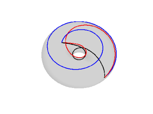
Figure 6: $(\mathcal{A}_{m})^{h}$ Geodesic curvature flow on a Clifford torus, with $\partial_{D}I=\partial I=\{0,1\}$. The solutions $\vec{X}^{m}$ at times $t=0,2,\ldots,6$. Below we visualise $\vec{\Phi}(\vec{X}^{m})$ at times $t=0$ (blue), $t=2$ (red) and $t=6$ (black), for (1.4e) with $\mathfrak{s}=1$, and also show a plot of the discrete energy $L_{g}^{h}(\vec{X}^{m})$.

On recalling Remark 4.4, we also present an evolution for geodesic curvature flow of a closed curve that is not homotopic to a point. See Figure 7 for a presentation of the numerical results for the scheme $(\mathcal{C}_{m,\star})^{h}$.

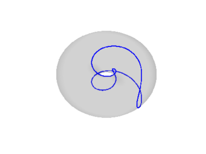
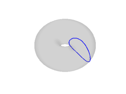
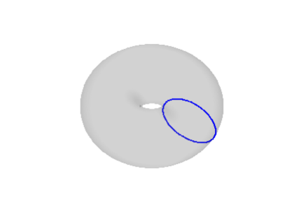
Figure 7: $(\mathcal{C}_{m,\star})^{h}$ Geodesic curvature flow on a Clifford torus. We visualise $\vec{\Phi}(\vec{X}^{m})$ at times $t=0,1,3$, for (1.4e) with $\mathfrak{s}=1$. A plot of the discrete energy $L_{g}^{h}(\vec{X}^{m})$ below.

5.3 The Angenent metric (1.5a)

Unless otherwise stated, we choose $n=2$ in (1.5a). First we show the evolution under curvature flow of an eongated cigar shape that shrinks to a point, see in Figure 8.

Figure 8: $(\mathcal{C}_{m,\star})^{h}$ Curvature flow towards extinction for (1.5a). Solution at times $t=0,0.1,0.2,0.25$.

In a second experiment, we show the evolution under elastic flow of a circle towards the generating curve of the Angenent torus in an axisymmetric setting. We recall that the Angenent torus is a critical point of Huisken’s $F$-functional (1.6), and hence a self-shrinker for mean curvature flow in ${\mathbb{R}}^{3}$, with extinction time 1. As a consequence, the generating curve of the Angenent torus, which from now on we will also simply call Angenent torus, is a critical point of the geodesic length $L_{g}$, and hence a geodesic. For the evolution shown in Figure 9, we observe that the discrete curvature energy $W_{g}^{m+1}$ reduces from about $3.5$ to about $10^{-5}$, giving a strong indication that we have indeed found a geodesic. Note also that the final shape in Figure 9 agrees well with the numerical results in [22, 17, 3].

Figure 9: $(\mathcal{Q}_{m})^{\star}$ Elastic flow for (1.5a) towards the Angenent torus. Plots are at times $t=0,0.1,0.5$. We also show a plot of the discrete energy $\widetilde{W}_{g}^{m+1}$ over time.

We have also performed simulations for elastic flow of initial curves with a winding number larger than one, with respect to the point $2\,\vec{e}_{1}$, and they always settle as a stationary solution on a multiple covering of the Angenent torus.

It is known that the Angenent torus is an unstable critical point of the geodesic length $L_{g}$, see [23, 54, 18], and this is confirmed by our numerical experiments. Hence it is practically impossible to obtain an approximation to it as a long-time limit of curvature flow. We demonstrate this phenomenon by starting two simulations for the stable scheme $(\mathcal{C}_{m,\star})^{h}$ from slightly shifted Angenent tori. Our numerical results in Figure 10 confirm that the stationary solution is unstable, and we see the curve either moving monotonically towards the $x_{2}$–axis, or towards infinity, with a significant decrease in the geodesic length of the curve in each case. For these experiments we used the finer discretisation parameters $J=2048$ and $\Delta t=10^{-5}$.

Figure 10: $(\mathcal{C}_{m,\star})^{h}$ Curvature flow for (1.5a), starting from horizontally shifted Angenent tori. Above shifted by $0.05$ to the right, below shifted by $0.05$ to the left. Plots are at times $t=0,0.18,0.2$ (above) and at times $t=0,0.02,0.03,0.038$ (below). We also show plots of the discrete energy $L_{g}^{h}(\vec{X}^{m})$ over time.

We highlight the capabilities of our numerical method by computing the “Angenent tori” in dimensions four and five, that is hypersurfaces in ${\mathbb{R}}^{n+1}$ that are topologically equivalent to ${\mathbb{S}}^{1}\times{\mathbb{S}}^{n-1}$, $n=3,4$, and that are self-shrinkers for mean curvature flow with extinction time 1. In particular, in Figure 11 we show the numerical steady states for approximations of elastic flow for the metric (1.5a), with $n=2,3,4$. In each case the final discrete energy satisfies $|\widetilde{W}_{g}^{M}|<10^{-9}$, confirming that we are indeed approximating geodesics.

Figure 11: $(\mathcal{Q}_{m})^{\star}$ Steady states for elastic flow for (1.5a) with $n=2,3,4$. Their discrete geodesic lengths are $3.70$, $6.39$ and $14.27$.

We note that in the study of mean curvature flow self-shrinkers the value of Huisken’s $F$-functional itself is also a relevant quantity of interest, see e.g. [61, 23, 35, 17]. For example, for a self-shrinker its value of $F$ is equal to its entropy. On recalling (1.6), (1.5a) and (2.8), we note that if $\vec{y}(\overline{I})\subset H$ is the generating curve for a rotationally symmetric hypersurface $\mathcal{S}\subset{\mathbb{R}}^{n+1}$, then

$$F(\mathcal{S})=(4\,\pi)^{-\frac{n}{2}}\,\mathcal{H}^{n-1}({\mathbb{S}}^{n-1})\left((\vec{y}\,.\,\vec{e}_{1})^{n-1}\,e^{-\frac{1}{4}\,|\vec{y}|^{2}},|\vec{y}_{\rho}|\right)=2^{1-n}\,[{\Gamma}(\tfrac{n}{2})]^{-1}\,L_{g}(\vec{y})\,.$$ (5.1)

Hence in order to deduce the value of Huisken’s $F$-functional for the self-shrinkers that we have found computationally, it is sufficient to report on the length of the corresponding geodesics, which we will do from now on within the captions of the relevant figures. Here we note that the pre-factor in (5.1) for the cases $n=2,3,4$ is given by $2^{1-n}\,[{\Gamma}(\tfrac{n}{2})]^{-1}=\frac{1}{2}$, $\frac{1}{2\,\sqrt{\pi}}$ and $\tfrac{1}{8}$, respectively. For the three geodesics displayed in Figure 11, our computed values for the final discrete length $L_{g}^{h}(\vec{X}^{M})$ are $3.70$, $6.39$ and $14.27$, giving approximate values for the entropy of the associated surfaces of revolution of $1.85$, $1.80$ and $1.78$, respectively. We remark that the value for $n=2$ agrees very well with the results reported in [17, 3].

Denoting the entropy of the $n$-dimensional “Angenent torus” with $E_{n}$, we have so far established that $E_{2}\approx 1.85$, $E_{3}\approx 1.80$ and $E_{4}\approx 1.78$. Continuing the above procedure for increasing values of $n$, we numerically obtain that $E_{6}\approx 1.77$, $E_{8}\approx 1.76$ and $E_{12}\approx 1.75$. This leads us to conjecture that $E_{n}$ is a strictly monotonically decreasing sequence with $E_{n}\searrow\sqrt{3}$ as $n\to\infty$. Note that this conjecture is in the spirit of Lemma A.4 in [61].

Of course, the most famous self-shrinker for mean curvature flow in ${\mathbb{R}}^{n+1}$, with extinction time 1, is the sphere of radius $\sqrt{2\,n}$, see e.g. [23]. In the context of the metric (1.5a), these correspond to geodesics in the shape of semicircles with radius $\sqrt{2\,n}$. For $n=2$ and $n=3$ we show an evolution each for elastic flow towards these geodesics, see Figure 12 for details, where in each case as initial data we choose a semicircle of radius $n-1$. For the two geodesics displayed in Figure 12, our computed values for the final discrete length $L_{g}^{h}(\vec{X}^{M})$ are $2.94$ and $5.15$, giving approximate values for the entropy of the associated spheres of $1.47$ and $1.45$. We remark that these values agree very well with the known values from [61, Examples A.3], which are known to converge to $\sqrt{2}$ as $n\to\infty$, recall [61, Lemma A.4].

Figure 12: $(\mathcal{Q}_{m})^{\star}$ Elastic flow for (1.5a), $n=2$ (left) and $n=3$ (right), and $\partial I=\partial_{0}I=\{0,1\}$. Solutions at times $t=0,0.1,1$ (left) and at times $t=0,0.1,1,3$ (right). We also show a plot of the discrete energy $\widetilde{W}_{g}^{m+1}$ over time. The discrete lengths of the obtained geodesics are $2.94$ ($n=2$) and $5.15$ ($n=3$).

In order to investigate the numerical accuracy of our proposed method, in Table 4 we compare the numerical steady state solutions of elastic flow in the case $n=2$ with a semicircle of radius $2$, as well as their respective induced entropy values. That is, we list the errors $\mathcal{E}^{M}=\max_{j=0,\ldots,J}|2-|\vec{X}^{M}(q_{j})||$ and $e^{M}=|\frac{1}{2}L_{g}^{h}(\vec{X}^{M})-\frac{4}{e}|$ for increasing values of $J$. Here we fix $T=10$ and $\Delta t=10^{-5}$, and always start from the approximation of a unit semicircle. The results presented in Table 4 appear to show a convergence rate of $1.5$ for the discrete $L^{\infty}$ error $\mathcal{E}^{M}$, while the entropy error $e^{M}$ appears to converge quadratically.

$J$	$\mathcal{E}^{M}$	EOC	$e^{M}$	EOC
32	1.9076e-02	—	1.4523e-03	—
64	6.7016e-03	1.51	3.7588e-04	1.95
128	2.3596e-03	1.51	9.5579e-05	1.98
256	8.3177e-04	1.50	2.4097e-05	1.99
512	2.9555e-04	1.49	6.0496e-06	1.99

Table 4: Errors and experimental orders of convergence for the convergence test corresponding to the final shape of the evolution on the left of Figure 12.

The final simulations in this subsection are devoted to finding self-shrinkers for mean curvature flow that are non-embedded, inspired by the work [34]. We begin with an experiment for a closed curve with seven self-intersections, see Figure 13. Under elastic flow the curve evolves towards the generating curve of a non-embedded self-shrinker for mean curvature flow. In fact, the steady state corresponds to the shape in [34, Figure 6]. Due to the large energy decrease at the beginning of the evolution, we use an adaptive time stepping strategy with $\Delta t_{\min}=10^{-7}$ and $\Delta t_{\max}=10^{-6}$. The spatial discretisation uses $J=512$. The discrete energy of the final solution satisfies $|\widetilde{W}^{M}_{g}|<10^{-9}$, confirming that we are indeed approximating a geodesic. We note that the discrete geodesic length of the final curve is $10.53$, giving an entropy of $5.26$.

Figure 13: $(\mathcal{Q}_{m})^{\star}$ Elastic flow for (1.5a). Solution at times $t=0,0.01$, $t=1$ and $t=20$. The discrete geodesic length of the final curve is $10.53$.

We also investigate, what happens to the geodesic from Figure 13 if we change the metric to (1.5a) with $n=3$. See Figure 14 for a plot of the obtained numerical result, which compared to the geodesic for $n=2$ has shifted further to the right. For this experiment we once again used an adaptive time stepping strategy. We note that the discrete energy of the final solution satisfies $|\widetilde{W}^{M}_{g}|<10^{-8}$. The discrete geodesic length of the final curve is $18.24$, giving an entropy of $5.15$.

Figure 14: $(\mathcal{Q}_{m})^{\star}$ Elastic flow for (1.5a) with $n=3$. Solution at times $t=0,1,100$. The discrete geodesic length of the final curve is $18.24$.

Inspired by [34, Figure 3], we now perform a numerical simulation to find a non-embedded self-shrinker of genus zero for mean curvature flow. Starting from an initial curve with three self-intersections, we observe the evolution for elastic flow shown in Figure 15, where the final discrete energy satisfies $|\widetilde{W}^{M}_{g}|<10^{-9}$. We note the excellent agreement with [34, Figure 3]. Here we again make use of an adaptive time stepping strategy with $\Delta t_{\min}=10^{-7}$ and $\Delta t_{\max}=10^{-4}$. The spatial discretisation uses $J=512$. We note that the discrete geodesic length of the final curve is $7.33$, giving an entropy of $3.66$.

Figure 15: $(\mathcal{Q}_{m})^{\star}$ Elastic flow for (1.5a) and $\partial I=\partial_{0}I=\{0,1\}$. Solution at times $t=0,0.01$, $t=0.1$ and $t=10$. The discrete geodesic length of the final curve is $7.33$.

5.4 The cone metric (1.5b)

In a first experiment for the metric (1.5b), we look at (geodesic) curvature flow for a curve on a cone with $\mathfrak{b}=0.5$, and so $\beta=3^{-\frac{1}{2}}$ in (1.7). For the simulation in Figure 16 it can be observed that in $H$ the initial circle of radius 2 deforms and shrinks to a point. On the hypersurface $\mathcal{M}=\vec{\Phi}(H)$, the initial curve is homotopic to a point, and so shrinks to a point away from the apex.

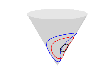
Figure 16: $(\mathcal{A}_{m})^{h}$ Geodesic curvature flow on a cone. The solutions $\vec{X}^{m}$ at times $t=0,0.5,1$. On the right we visualise $\vec{\Phi}(\vec{X}^{m})$ at times $t=0,0.5,1$, for (1.5b) with $\mathfrak{b}=0.5$. A plot of the discrete energy $L_{g}^{h}(\vec{X}^{m})$ is shown on the right.

The following conjecture on geodesic curvature flow on a cone was formulated by Charles M. Elliott, [36].

Conjecture. 5.1.

A closed curve on a cone $\mathcal{M}$, that is not homotopic to a point on $\mathcal{M}$, will under geodesic curvature flow converge to the apex in finite time.

The conjecture says, in particular, that the singularity of the flow will happen at the apex. Indeed we expect that all the points of the curve converge to the apex at the singular time. Moreover, we expect that a similar conjecture holds on more general surfaces on which a curve encloses a singularity.

On recalling Remark 4.4, we now numerically test the conjecture by starting an evolution for geodesic curvature flow with a closed curve that is very close to the apex, but not uniformly so. That is, we vary the $x_{2}$–coordinate of the initial curve in $H$ between $\pm 2$. During the evolution, the parts of the curve closest to the apex first start to rise, making the curve becoming more circle-like, before the whole curve sinks towards to apex. See Figure 17, where we also show a plot of the lowest point of the curve on the cone over time, highlighting the rise and fall of the curve on the cone. The observed behaviour is consistent with Conjecture 5.1

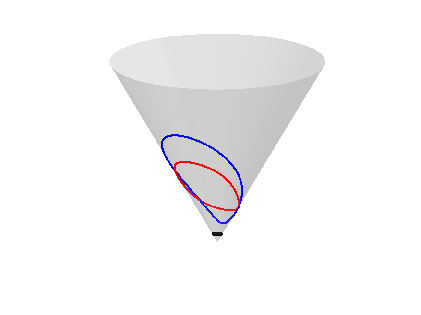
Figure 17: $(\mathcal{A}_{m})^{h}$ Geodesic curvature flow on a cone. We visualise $\vec{\Phi}(\vec{X}^{m})$ at times $t=0,0.5,1.5$, for (1.5b) with $\mathfrak{b}=0.5$. A plot of the discrete energy $L_{g}^{h}(\vec{X}^{m})$ over the time interval $[0,1.52]$ in the middle. On the right a plot of the lowest point of the curve on the cone, $\exp(\mathfrak{b}\,\min_{\overline{I}}\vec{X}^{m}\,.\,\vec{e}_{1})$.

An experiment for (geodesic) elastic flow on the same cone is shown in Figure 18. Here the closed curve first approaches a circle, which then rises along the cone. By computing the energy one observes that a circle with increasing radius reduces the elastic energy.

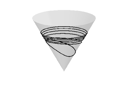
Figure 18: $(\mathcal{Q}_{m,\star})^{h}$ Geodesic elastic flow on a cone. We visualise $\vec{\Phi}(\vec{X}^{m})$ at times $t=0,10,\ldots,50$, for (1.5b) with $\mathfrak{b}=0.5$. A plot of the discrete energy $\widetilde{W}_{g}^{m+1}$ on the right.

5.5 The metric (1.5c)

We end the section on the numerical results for our presented schemes with some simulations for the metric (1.5c) with (1.8) and (1.9). Recall that now geodesics in $H$ correspond to optimal interface profiles in multi-component phase field models. Of particular interest are geodesics, or shortest paths, that connect the vertices ${\bf e}_{1}$, ${\bf e}_{2}$, ${\bf e}_{3}$ of the Gibbs simplex G, recall (1.10). To this end, we note that with the choice (1.8), it holds that the map $\vec{z}\mapsto f(\vec{z})={\bf u}_{0}+U\,\vec{z}$ satisfies $f(0,0)={\bf e}_{1}$, $f(-2^{\frac{1}{2}},0)={\bf e}_{2}$ and $f(-2^{\frac{1}{2}},-(\frac{3}{2})^{\frac{1}{2}})={\bf e}_{3}$. For the first experiment we set $(\sigma_{12},\sigma_{13},\sigma_{23},\sigma_{123})=(4,6,9,0)$, and numerically compute a geodesic connecting ${\bf e}_{1}$ and ${\bf e}_{2}$ with the help of geodesic curvature flow. Here we always use the scheme $(\mathcal{A}_{m})^{h}$ with the uniform time step size $\Delta t=10^{-5}$. The results are shown in Figure 19, where we see that the flow quickly settles on a curved geodesic. We repeat the same simulation also for the paths connecting the pure phases ${\bf e}_{1}$ and ${\bf e}_{3}$, as well as ${\bf e}_{2}$ and ${\bf e}_{3}$, and plot all three solutions within the Gibbs simplex $G$, recall (1.10), at the bottom of Figure 19.

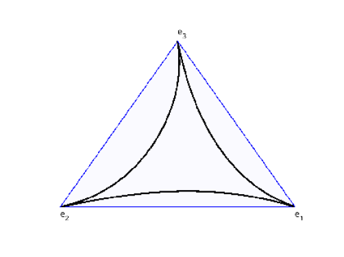
Figure 19: $(\mathcal{A}_{m})^{h}$ Geodesic curvature flow for the metric (1.5c) with (1.9) and $(\sigma_{12},\sigma_{13},\sigma_{23},\sigma_{123})=(4,6,9,0)$. The solutions $\vec{X}^{m}$ at times $t=0,0.01,0.1$. A plot of the discrete energy $L_{g}^{h}(\vec{X}^{m})$ on the right. Below a plot of the three minimisers connecting the vertices of the Gibbs simplex.

In [41] numerical computations indicated that on choosing $\sigma_{123}>0$ in (1.9) larger and larger, the minimising profiles can be forced to approach the edges of the Gibbs simplex. To confirm this effect with our numerical method, we now choose $\sigma_{123}\in\{10,100,1000\}$ and plot the obtained geodesics in Figure 20. It can be seen that for an increasing value of $\sigma_{123}$, the geodesics are pushed further and further towards the edges of the Gibbs simplex.

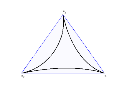
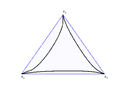
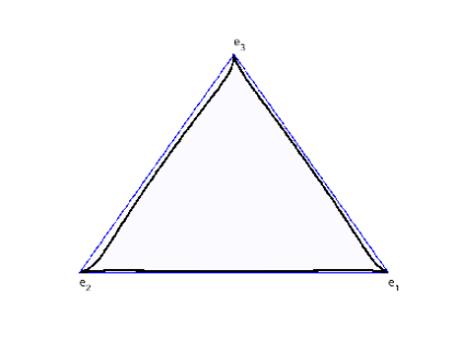
Figure 20: $(\mathcal{A}_{m})^{h}$ The minimisers obtained within the Gibbs simplex, for (1.9) with $(\sigma_{12},\sigma_{13},\sigma_{23})=(4,6,9)$ and $\sigma_{123}=10,100,1000$ (from left to right).

We remark that in [19] a novel approach for multi-component phase field models has been considered, where the Ginzburg–Landau energy can be defined such that the minimising paths connecting the pure phases are always given by the edges of the Gibbs simplex. The metric that would arise in the form of (1.5c) in order to model this situation is in general no longer conformal, and so would be outside the context of this paper. However, following the approach in [42, 38], we can consider the following replacement of (1.9) to achieve the same effect:

$$\Psi(u_{1},u_{2},u_{3})=\sigma_{12}\,u_{1}^{2}\,u_{2}^{2}+\sigma_{13}\,u_{1}^{2}\,u_{3}^{2}+\sigma_{23}\,u_{2}^{2}\,u_{3}^{2}+\widehat{\sigma}_{123}\,u_{1}\,u_{2}\,u_{3}^{2}+\widehat{\sigma}_{231}\,u_{2}\,u_{3}\,u_{1}^{2}+\widehat{\sigma}_{312}\,u_{3}\,u_{1}\,u_{2}^{2}\,,$$ (5.2)

where $\widehat{\sigma}_{123},\widehat{\sigma}_{231},\widehat{\sigma}_{312}\in{\mathbb{R}}_{\geq 0}$. We perform a computation for (5.2) with $\sigma_{12}=\sigma_{13}=\sigma_{23}=\widehat{\sigma}_{123}=\widehat{\sigma}_{231}=\widehat{\sigma}_{312}=1$ and show the obtained results in Figure 21. It can be seen that now the geodesics lie on the edges of the Gibbs simplex, confirming the analysis in [42, 38].

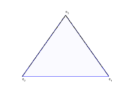
Figure 21: $(\mathcal{A}_{m})^{h}$ The minimisers obtained for (5.2) with $\sigma_{12}=\sigma_{13}=\sigma_{23}=\widehat{\sigma}_{123}=\widehat{\sigma}_{231}=\widehat{\sigma}_{312}=1$ are precisely the edges of the Gibbs simplex.

Acknowledgements
The authors gratefully acknowledge the support of the Regensburger Universitätsstiftung Hans Vielberth.

References

• [1] B. Andrews and X. Chen, Curvature flow in hyperbolic spaces, J. Reine Angew. Math., 729 (2017), pp. 29–49.
• [2] S. B. Angenent, Shrinking doughnuts, in Nonlinear diffusion equations and their equilibrium states, 3 (Gregynog, 1989), vol. 7 of Progr. Nonlinear Differential Equations Appl., Birkhäuser Boston, Boston, MA, 1992, pp. 21–38.
• [3] J. W. Barrett, K. Deckelnick, and R. Nürnberg, A finite element error analysis for axisymmetric mean curvature flow, IMA J. Numer. Anal., (2020). (to appear).
• [4] J. W. Barrett, H. Garcke, and R. Nürnberg, On the variational approximation of combined second and fourth order geometric evolution equations, SIAM J. Sci. Comput., 29 (2007), pp. 1006–1041.
• [5]  , A parametric finite element method for fourth order geometric evolution equations, J. Comput. Phys., 222 (2007), pp. 441–462.
• [6]  , Numerical approximation of gradient flows for closed curves in ${\mathbb{R}}^{d}$, IMA J. Numer. Anal., 30 (2010), pp. 4–60.
• [7]  , Elastic flow with junctions: Variational approximation and applications to nonlinear splines, Math. Models Methods Appl. Sci., 22 (2012), p. 1250037.
• [8]  , Parametric approximation of isotropic and anisotropic elastic flow for closed and open curves, Numer. Math., 120 (2012), pp. 489–542.
• [9]  , Finite element methods for fourth order axisymmetric geometric evolution equations, J. Comput. Phys., 376 (2019), pp. 733–766.
• [10]  , Stable discretizations of elastic flow in Riemannian manifolds, SIAM J. Numer. Anal., 57 (2019), pp. 1987–2018.
• [11]  , Variational discretization of axisymmetric curvature flows, Numer. Math., 141 (2019), pp. 791–837.
• [12]  , Numerical approximation of curve evolutions in Riemannian manifolds, IMA J. Numer. Anal., 40 (2020), pp. 1601–1651.
• [13]  , Parametric finite element approximations of curvature driven interface evolutions, in Handb. Numer. Anal., A. Bonito and R. H. Nochetto, eds., vol. 21, Elsevier, Amsterdam, 2020, pp. 275–423.
• [14]  , Stable approximations for axisymmetric Willmore flow for closed and open surfaces, M2AN Math. Model. Numer. Anal., 55 (2021), pp. 833–885.
• [15] S. Bartels, A simple scheme for the approximation of the elastic flow of inextensible curves, IMA J. Numer. Anal., 33 (2013), pp. 1115–1125.
• [16] H. Benninghoff and H. Garcke, Segmentation and restoration of images on surfaces by parametric active contours with topology changes, J. Math. Imaging Vision, 55 (2016), pp. 105–124.
• [17] Y. Berchenko-Kogan, The entropy of the Angenent torus is approximately 1.85122, Experiment. Math., (2019). (to appear).
• [18]  , Numerically computing the index of mean curvature flow self-shrinkers. arXiv: 2007.06094, 2020.
• [19] E. Bretin and S. Masnou, A new phase field model for inhomogeneous minimal partitions, and applications to droplets dynamics, Interfaces Free Bound., 19 (2017), pp. 141–182.
• [20] E. Cabezas-Rivas and V. Miquel, Volume preserving mean curvature flow in the hyperbolic space, Indiana Univ. Math. J., 56 (2007), pp. 2061–2086.
• [21] L.-T. Cheng, P. Burchard, B. Merriman, and S. Osher, Motion of curves constrained on surfaces using a level-set approach, J. Comput. Phys., 175 (2002), pp. 604–644.
• [22] D. L. Chopp, Computation of self-similar solutions for mean curvature flow, Experiment. Math., 3 (1994), pp. 1–15.
• [23] T. H. Colding and W. P. Minicozzi II, Generic mean curvature flow I: generic singularities, Ann. of Math. (2), 175 (2012), pp. 755–833.
• [24] A. Dall’Acqua, T. Laux, C.-C. Lin, P. Pozzi, and A. Spener, The elastic flow of curves on the sphere, Geom. Flows, 3 (2018), pp. 1–13.
• [25] A. Dall’Acqua, C.-C. Lin, and P. Pozzi, Evolution of open elastic curves in $\mathbb{R}^{n}$ subject to fixed length and natural boundary conditions, Analysis (Berlin), 34 (2014), pp. 209–222.
• [26]  , A gradient flow for open elastic curves with fixed length and clamped ends, Ann. Sc. Norm. Super. Pisa Cl. Sci. (5), 17 (2017), pp. 1031–1066.
• [27]  , Elastic flow of networks: long-time existence result, Geom. Flows, 4 (2019), pp. 83–136.
• [28] A. Dall’Acqua and P. Pozzi, A Willmore-Helfrich $L^{2}$-flow of curves with natural boundary conditions, Comm. Anal. Geom., 22 (2014), pp. 617–669.
• [29] A. Dall’Acqua and A. Spener, The elastic flow of curves in the hyperbolic plane. arXiv:1710.09600, 2017.
• [30]  , Circular solutions to the elastic flow in hyperbolic space, in Proceedings of Analysis on Shapes of Solutions to Partial Differential Equations, (2017), vol. 2082 of RIMS Kôkyûroku, Kyoto, Japan, 2018.
• [31] T. A. Davis, Algorithm 832: UMFPACK V4.3—an unsymmetric-pattern multifrontal method, ACM Trans. Math. Software, 30 (2004), pp. 196–199.
• [32] K. Deckelnick and G. Dziuk, Error analysis for the elastic flow of parametrized curves, Math. Comp., 78 (2009), pp. 645–671.
• [33] K. Deckelnick, G. Dziuk, and C. M. Elliott, Computation of geometric partial differential equations and mean curvature flow, Acta Numer., 14 (2005), pp. 139–232.
• [34] G. Drugan and S. J. Kleene, Immersed self-shrinkers, Trans. Amer. Math. Soc., 369 (2017), pp. 7213–7250.
• [35] G. Drugan and X. H. Nguyen, Shrinking doughnuts via variational methods, J. Geom. Anal., 28 (2018), pp. 3725–3746.
• [36] C. M. Elliott, Private communication, 2009.
• [37] C. L. Epstein and M. Gage, The curve shortening flow, in Wave motion: theory, modelling, and computation (Berkeley, Calif., 1986), vol. 7 of Math. Sci. Res. Inst. Publ., Springer, New York, 1987, pp. 15–59.
• [38] H. Garcke and R. Haas, Modeling of Nonisothermal Multi-Component, Multi-Phase Systems with Convection, John Wiley & Sons, Ltd, 2008, ch. 20, pp. 325–338.
• [39] H. Garcke, J. Menzel, and A. Pluda, Willmore flow of planar networks, J. Differential Equations, 266 (2019), pp. 2019–2051.
• [40]  , Long time existence of solutions to an elastic flow of networks, Comm. Partial Differential Equations, 45 (2020), pp. 1253–1305.
• [41] H. Garcke, B. Stoth, and B. Nestler, A multiphase field concept: numerical simulations of moving phase boundaries and multiple junctions, SIAM J. Appl. Math., 60 (1999), pp. 295–315.
• [42] R. Haas, Modeling and Analysis for general non-isothermal convective Phase Field Systems, PhD thesis, University Regensburg, Regensburg, 2007.
• [43] M. Helmers, Kinks in two-phase lipid bilayer membranes, Calc. Var. Partial Differential Equations, 48 (2013), pp. 211–242.
• [44]  , Convergence of an approximation for rotationally symmetric two-phase lipid bilayer membranes, Q. J. Math., 66 (2015), pp. 143–170.
• [45] G. Huisken, Asymptotic behavior for singularities of the mean curvature flow, J. Differential Geom., 31 (1990), pp. 285–299.
• [46] J. Jost, Riemannian Geometry and Geometric Analysis, Springer-Verlag, Berlin, 2005.
• [47] S. Kleene and N. M. Møller, Self-shrinkers with a rotational symmetry, Trans. Amer. Math. Soc., 366 (2014), pp. 3943–3963.
• [48] N. Koiso, On motion of an elastic wire in a Riemannian manifold and singular perturbation, Osaka J. Math., 52 (2015), pp. 453–473.
• [49] D. Kraus and O. Roth, Conformal metrics, in Topics in Modern Function Theory, vol. 19 of Ramanujan Math. Soc. Lect. Notes Ser., Ramanujan Math. Soc., Mysore, India, 2013, pp. 41–83. (see also https://arxiv.org/abs/0805.2235).
• [50] W. Kühnel, Differential Geometry: Curves – Surfaces – Manifolds, vol. 77 of Student Mathematical Library, Amer. Math. Soc., Providence, RI, 2015.
• [51] J. Langer and D. A. Singer, The total squared curvature of closed curves, J. Differential Geom., 20 (1984), pp. 1–22.
• [52]  , Curve-straightening in Riemannian manifolds, Ann. Global Anal. Geom., 5 (1987), pp. 133–150.
• [53] A. Linnér, Curve-straightening and the Palais-Smale condition, Trans. Amer. Math. Soc., 350 (1998), pp. 3743–3765.
• [54] Z. H. Liu, The Morse index of mean curvature flow self-shrinkers, PhD thesis, Massachusetts Institute of Technology, Ann Arbor, MI, 2016.
• [55] E. Maitre and F. Santosa, Level set methods for optimization problems involving geometry and constraints. II. Optimization over a fixed surface, J. Comput. Phys., 227 (2008), pp. 9596–9611.
• [56] K. Mikula and D. Ševčovič, Evolution of curves on a surface driven by the geodesic curvature and external force, Appl. Anal., 85 (2006), pp. 345–362.
• [57] M. Müller and A. Spener, On the Convergence of the Elastic Flow in the Hyperbolic Plane, Geom. Flows, 5 (2020), pp. 40–77.
• [58] E. Schippers, The calculus of conformal metrics, Ann. Acad. Sci. Fenn. Math., 32 (2007), pp. 497–521.
• [59] A. Schmidt and K. G. Siebert, Design of Adaptive Finite Element Software: The Finite Element Toolbox ALBERTA, vol. 42 of Lecture Notes in Computational Science and Engineering, Springer-Verlag, Berlin, 2005.
• [60] A. Spira and R. Kimmel, Geometric curve flows on parametric manifolds, J. Comput. Phys., 223 (2007), pp. 235–249.
• [61] A. Stone, A density function and the structure of singularities of the mean curvature flow, Calc. Var. Partial Differential Equations, 2 (1994), pp. 443–480.