P³-LOAM: PPP/LiDAR Loosely Coupled SLAM with Accurate Covariance Estimation and Robust RAIM in Urban Canyon Environment

Abstract

Light Detection and Ranging (LiDAR) based Simultaneous Localization and Mapping (SLAM) has drawn increasing interests in autonomous driving. However, LiDAR-SLAM suffers from accumulating errors which can be significantly mitigated by Global Navigation Satellite System (GNSS). Precise Point Positioning (PPP), an accurate GNSS operation mode independent of base stations, gains growing popularity in unmanned systems. Considering the features of the two technologies, LiDAR-SLAM and PPP, this paper proposes a SLAM system, namely P³-LOAM (PPP based LiDAR Odometry and Mapping) which couples LiDAR-SLAM and PPP. For better integration, we derive LiDAR-SLAM positioning covariance by using Singular Value Decomposition (SVD) Jacobian model, since SVD provides an explicit analytic solution of Iterative Closest Point (ICP), which is a key issue in LiDAR-SLAM. A novel method is then proposed to evaluate the estimated LiDAR-SLAM covariance.

In addition, to increase the reliability of GNSS in urban canyon environment, we develop a LiDAR-SLAM assisted GNSS Receiver Autonomous Integrity Monitoring (RAIM) algorithm. Finally, we validate P³-LOAM with UrbanNav, a challenging public dataset in urban canyon environment. Comprehensive test results prove that, in terms of accuracy and availability, P³-LOAM outperforms benchmarks such as Single Point Positioning (SPP), PPP, LeGO-LOAM, SPP-LOAM, and the loosely coupled navigation system proposed by the publisher of UrbanNav.

I Introduction

Light Detection and Ranging based Simultaneous Localization and Mapping (LiDAR-SLAM) systems including 2D and 3D LiDAR-SLAM have been studied for decades. 2D LiDAR-SLAM comprises FastSLAM [1], Hector-SLAM [2], GMapping [3], KartoSLAM [4], LagoSLAM (Linear Approximation for Graph-based SLAM) [5] and so on, while 3D LiDAR-SLAM includes LOAM (LiDAR Odometry and Mapping) [6], LeGO-LOAM (Lightweight and Ground-Optimized LiDAR Odometry and Mapping) [7], Suma [8], and Suma++ [9], among others. These advanced systems aim to achieve self-motion estimation with low drift and high precision in the areas which require accurate positioning. In general, though the cost of 3D LiDAR-SLAM is much higher, it is much more accurate and robust than 2D LiDAR-SLAM, especially in large-scale outdoor environment where 2D LiDAR-SLAM generally fails to work. Therefore, we focus on 3D LiDAR-SLAM in this paper.

Currently, the LiDAR-SLAM framework mainly involves two parts: frontend and backend. The frontend registers two frames of point cloud data and then obtains the transformation matrix. The frontend primarily includes three kinds of algorithms: Iterative Closest Point (ICP) [10] as well as its extensions [11], [12], Correlation Scan Matching (CSM) [13], and Normal Distributions Transform (NDT) [14].

As for the backend of LiDAR-SLAM, it serves to mitigate errors accumulated from the frontend. Early studies utilized filtering methods such as Extended Kalman Filtering (EKF) [15], Unscented Kalman Filtering (UKF) [16] and Particle Filtering (PF) [17] in the backend of SLAM. The above mentioned Hector-SLAM used the EKF algorithm framework, while FastSLAM and Gmapping adopted PF algorithm architecture. Later studies began to explore optimization-based SLAM algorithm and achieved better performance. The KartoSLAM, LagoSLAM, LOAM, LeGO-LOAM, IMLS-SLAM, Suma, and Suma++ all used the optimization algorithm in their backends. Our previous study also utilized the optimization method to build a pose graph in a LiDAR-SLAM system [18].

Research concerning Global Navigation Satellite System (GNSS) has lasted for decades since the advent of Global Positioning System (GPS). GNSS includes GPS, GLONASS, Galileo and BeiDou. Its operation modes mainly involve four types: Single Point Positioning (SPP), Real-Time Differential (RTD) Positioning, Real-Time Kinematic (RTK) Positioning [19] and Precise Point Positioning (PPP) [20]. The positioning accuracy would be affected by many factors including receiver clock errors, satellite clock errors, tropospheric delays, ionospheric delays, hardware code and phase biases, multipath errors, tide, antenna phase center, phase winding, earth rotation, relativity effects, etc. The ionospheric error is of significance for single-frequency GNSS users [21].

The characteristics of the four GNSS operation modes will be introduced below. SPP uses pseudorange and Doppler observation to locate and measure velocity. Due to the heavy noise of pseudorange itself, the SPP generally fixes errors above the meter level, including satellite clock errors, relativistic effects, tropospheric delay, ionospheric errors, and earth rotation. Generally, in SPP, the tropospheric error is corrected by empirical models like Hopfield [22] and Saastamoinen [23]; the ionospheric error is modified by Klobuchar model [24]; the satellite orbit error and clock error are both corrected by broadcast ephemeris; relativistic effects are corrected according to the model; earth rotation errors can be corrected according to the signal propagation time. RTD uses reference stations with known fixed positions to calculate the differences between the measured pseudoranges and actual pseudoranges. The differences are then broadcast to nearby mobile stations for use. RTK corrects not only the pseudorange observation errors but also the phase observation errors, so as to obtain the positioning accuracy of centimeter level. RTD and RTK both need base stations. In contrast, PPP technology is more suitable for unmanned systems as PPP is independent of base stations. Single-frequency PPP (SF-PPP) and Dual-frequency PPP (DF-PPP) are two mainstream PPP technologies. Both of them need precise corrections which can be acquired from International GNSS Service Real-Time Service (IGS-RTS) [25] for the satellite orbits and satellite clocks. In autonomous driving, SF-PPP receives considerable attention because of its lower cost. However, the positioning performance of any GNSS modes will be affected by the coarse errors introduced by multipath and non-line-of-sight (NLOS) signals [26]. The observations with coarse errors are defined as GNSS outliers which can be eliminated by GNSS Receiver Autonomous Integrity Monitoring (RAIM) [27]. In recent years, multi-sensors assisted RAIM algorithms have been proposed [28], [29]. For example, inertial measurement unit (IMU) was used in RAIM with a tightly-coupled GNSS/INS(Inertial Navigation System) framework [30]. Our previous work also used LiDAR to analyze line-of-sight GNSS observations [31].

In autonomous driving, LiDAR-SLAM registers the point cloud to obtain the transformation matrix between two frames, then the trajectory is obtained, and maps are built accordingly. In this process, the error of LiDAR-SLAM inevitably occurs along with the distance drift. And in the open areas with limited features, LiDAR-SLAM may fail to work while GNSS performs well. Moreover, it is impossible to estimate the position in the earth coordinate system if we simply use the LiDAR-SLAM technology. This makes some navigation tasks more challenging. For these reasons, the coupling of GNSS will enable the LiDAR-SLAM system to provide more robust localization and mapping results with global earth coordinates in large-scale scenarios. In turn, GNSS is heavily influenced by multipath and NLOS in urban canyon environment, resulting in poor performance. LiDAR-SLAM always performs well in urban canyon environment and gets a relative positioning result. So it is meaningful to fuse GNSS and LiDAR-SLAM: LiDAR-SLAM can improve the reliability and availability of GNSS, on the other hand, GNSS can turn the positioning result of LiDAR-SLAM in a local coordinate system to the global such as World Geodetic System 1984 (WGS-84). But in conventional GNSS and LiDAR-SLAM fusion systems, few works have paid attention to either the calculation of LiDAR-SLAM positioning covariance, or the use of PPP in autonomous driving. In conclusion, our motivation for this paper is complementing PPP and LiDAR-SLAM to obtain more reliable and available positioning results in global coordinate system.

The main contributions of this paper are as follows:

1) Covariance is essential for weighting different positioning sources in a multi-sensor integrated localization approach. However, few LiDAR-SLAM systems provide covariance estimation since only one sensor is utilized. For more accurate integration of LiDAR-SLAM and PPP, we derive an SVD Jacobian based error propagation model to estimate the covariance of LiDAR-SLAM. The estimated result is evaluated by a novel method we propose, using GNSS covariance and ground truth of trajectory. The evaluation proves that the estimated LiDAR-SLAM covariance is reasonable.

2) Urban canyon environment always introduces GNSS observations with more coarse errors which may result in the failure of RAIM. In such an environment, LiDAR might provide more stable positioning results. Therefore, we propose a LiDAR-SLAM assisted GNSS RAIM to eliminate PPP outliers, achieving reliable GNSS positioning results. The max error of PPP is reduced to the same level as LiDAR-SLAM.

3) By applying the above SVD Jacobian based error propagation model and LiDAR-SLAM assisted GNSS RAIM, we develop a novel loosely coupled SLAM system called P³-LOAM. Then P³-LOAM was evaluated by UrbanNav, a challenging public dataset in urban canyon environment. P³-LOAM significantly outperforms benchmarks in terms of accuracy and availability.

The remaining paper is organized as follows. Section ii@ presents an overview of related work. Summary of the proposed architecture and algorithm is provided in Section iii@. Section iv@ describes the experimental setup and presents the results. Finally, conclusions are drawn in Section v@.

II Related work

Lots of studies have integrated GNSS and LiDAR-SLAM for better localization performance. LiDAR-SLAM positioning covariance was considered in Shetty et al.’s work [32], by modeling the positioning error as a Gaussian distribution and estimating the covariance from individual surface and edge feature points. This paper hypothesized that each surface feature point contributed to reducing positioning error in the direction of the corresponding surface normal, while each edge feature point helped in reducing position error in the direction perpendicular to the edge vector. But the eigenvalues of covariance matrix were fixed in this algorithm, so it is not adaptive for real-world circumstances where the eigenvalues would change with distance. Shetty et al. used Kalman Filtering to fuse LiDAR-SLAM and GNSS [32]. For transforming LiDAR-SLAM position to the global frame, their paper used an on-board attitude and heading reference system (AHRS) combined with an IMU. Constant velocity model was chosen as the dynamic model of Kalman Filtering, but the error propagation model of IMU would be a better choice in this case. Similarly, Pereira et al. [33] used GNSS, LiDAR and AHRS to navigate through the forest by constructing UKF. In contrast, IMU was used sufficiently through IMU preintegration [34]. However, its backend was not filtering but optimization method, and the covariance of LiDAR-SLAM was not considered. In addition, the LiDAR-SLAM algorithm in [34] was Cartographer, which is designed for indoor environment instead of urban canyon environment. We choose LOAM series LiDAR-SLAM algorithm in our paper as it obtains better localization performance on KITTI [35]. Qian et al. [36] used EKF to fuse RTK, IMU, and 2D LiDAR. They proved LiDAR could improve RTK ambiguity resolution. Qian et al argued that IMU could only keep high accuracy for a short time because of its drift errors while LiDAR could perform better. Similarly, 3D LiDAR was also fused with RTK and IMU using EKF in [37]. In the works above, IMU is crucial in converting global and local coordinates, but it is actually not a necessary component, as exemplified in [38], [39], [40] and [41]. Joerger et al. [38] used Kalman Filtering to fuse 2D LiDAR and GPS, resulting in a robust localization in forest scenario and urban canyon scenario. It is worth mentioning that Carrier-Phase Differential GPS was used in [38]. Shamsudin et al. [42] extended Rao-Blackwellized particle filtering to fuse RTK and 3D LiDAR. He et al. [39] used an optimization-based algorithm to integrate RTK and 3D LiDAR in partially GNSS-denied environment. In [40], the authors used a RAIM framework to integrate LiDAR odometry and GNSS by UKF. Hsu et al. [41] focused on GNSS covariance and applied Gaussian Mixture Model (GMM) to identify non-Gaussian GNSS outliers in SPP algorithm. The results were satisfactory by integrating SPP and LiDAR-SLAM, but there was still room for improvement. We therefore propose to utilize PPP technology and consider LiDAR-SLAM covariance in search for better results.

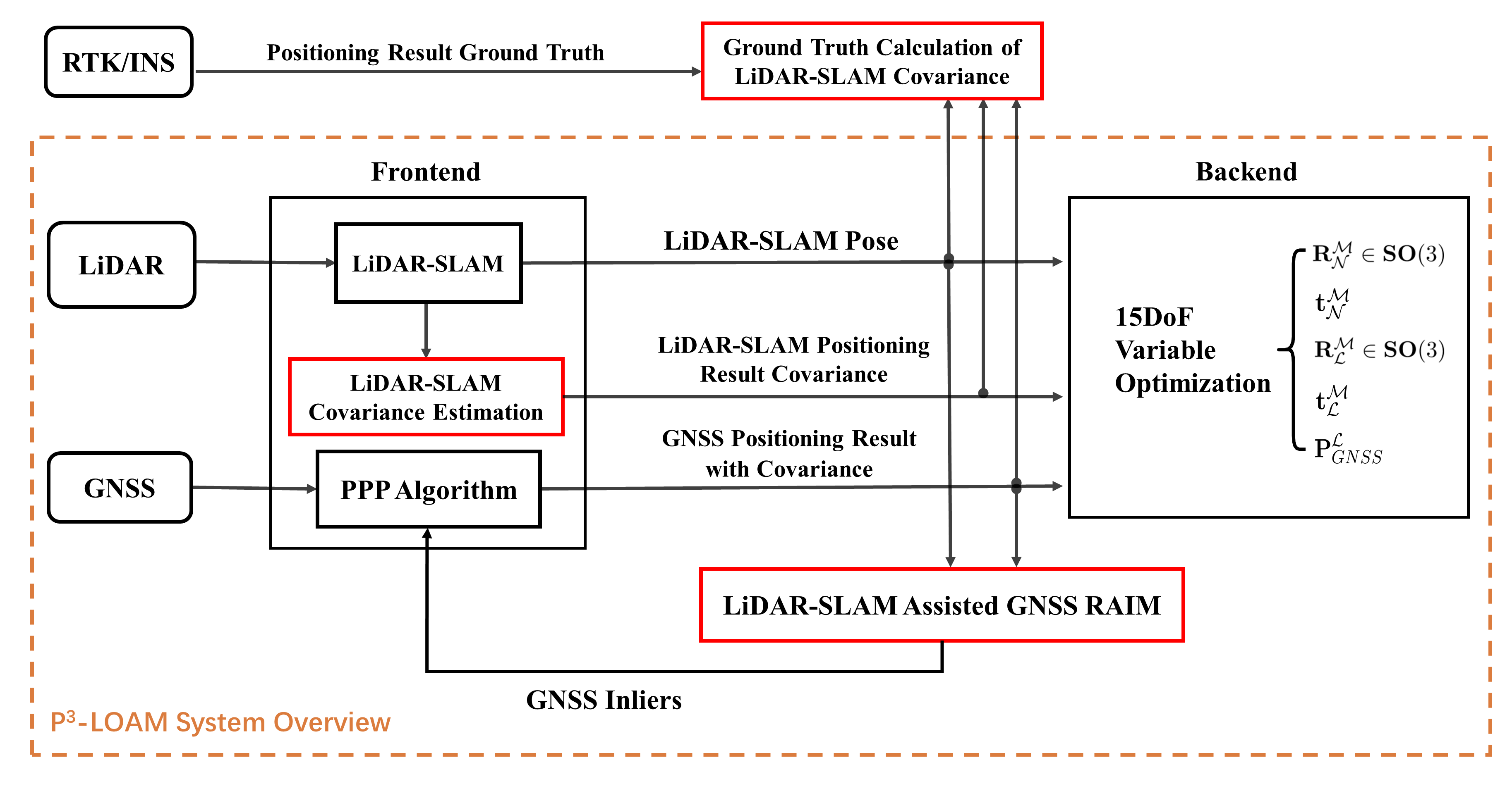
Figure 1: Overview of the Modules Involved

III Methodology

In this section, the specific implementation of P³-LOAM will be presented first. Secondly, we will briefly introduce the ICP algorithm and derive its error propagation based on SVD Jacobian model. Thirdly, the implementation of PPP algorithm and its covariance will be explicated. On this basis, the calculation method of LiDAR-SLAM covariance’s ground truth will be derived. Next, the LiDAR-SLAM assisted GNSS RAIM algorithm will also be proposed. At last, we will build up the factor graph model of the backend.

III-A Overview

All the modules involved in this paper are presented in Fig. 1. The content within the dashed box is the general architecture of the proposed P³-LOAM, and the outside part is a method to calculate the ground truth of LiDAR-SLAM covariance. P³-LOAM is divided into frontend and backend. In the frontend, LiDAR-SLAM and PPP algorithm are the two main modules. In the LiDAR-SLAM module, we add a covariance estimation. In the PPP module, we propose a RAIM to select GNSS inliers with the help of LiDAR-SLAM pose and PPP result. At last, a backend with 15DoF variable optimization is realized. The parts in Fig. 1 with red rectangles represent the contributions of our work.

The coordinate frames and notations involved in this article will be clarified below. The Earth-centered Earth-fixed coordinate system (ECEF, Frame $\mathcal{E}$, see Fig. 2) rotates with the Earth, taking the Earth’s centroid as the origin. The X-axis of Frame $\mathcal{E}$ points to the intersection of the equator and prime meridian. The Earth’s rotation axis is taken as Z-axis, and the North Pole is the positive direction. Then, the Y-axis is perpendicular to the X-Z plane, forming a right-handed coordinate system. The GNSS receiver generally outputs positioning results in Frame $\mathcal{E}$.

The East-North-Up coordinate system (ENU) is marked as Frame $\mathcal{N}$. When Frame $\mathcal{N}$ is used, we have to choose a point on the Earth as the origin. And the X-Y plane of Frame $\mathcal{N}$ is the local horizontal plane of the origin, with the X-axis being the tangential line of the latitude line that points East, and the Y-axis being the tangential line of the longitude line that points North. The Z-axis is perpendicular to the X-Y plane, forming a right-handed coordinate system.

The LiDAR frame is marked as Frame $\mathcal{L}$, with LiDAR’s center being the origin. The X-axis points to the right along the LiDAR horizontal axis, the Z-axis points forward along the LiDAR longitudinal axis, and the Y-axis is perpendicular to the X-Z plane, forming a right-handed coordinate system.

A local map frame is marked as Frame $\mathcal{M}$, coinciding with Frame $\mathcal{L}$ at the beginning and then keeps still.

For convenience of reading, we summarize all the involved coordinate frames and notations in Table I.

TABLE I: Coordinate Frames and Notations

$\mathcal{E}$	ECEF	$\mathcal{N}$	ENU Frame
$\mathcal{L}$	LiDAR Frame	$\mathcal{M}$	Locam Map Frame
$\mathbf{R}_{\mathcal{A}}^{\mathcal{B}}$	Rotation Matrix from Frame $\mathcal{A}$ to Frame $\mathcal{B}$	$\delta\theta_{\mathcal{A}}^{\mathcal{B}}$	Small disturbance to the left of $\mathbf{R}_{\mathcal{A}}^{\mathcal{B}}$
$\mathbf{t}_{\mathcal{A}}^{\mathcal{B}}$	Translation Vector from Frame $\mathcal{A}$ to Frame $\mathcal{B}$	$\delta\mathbf{t}_{\mathcal{A}}^{\mathcal{B}}$	Small disturbance to the left of $\mathbf{t}_{\mathcal{A}}^{\mathcal{B}}$
$\mathbf{P}_{\mathbf{G}}^{\mathcal{A}}$	The point $\mathbf{G}$’s coordinates in Frame $\mathcal{A}$	$Cov(\mathbf{X})$ or $\mathbf{\Lambda_{X}}$	Covariance of $\mathbf{X}$
$\mathbf{U}_{jk}$	The $j$th row and the $k$th column of matrix $\mathbf{U}$	$\mathbf{\Omega}$${}^{ij}_{\mathbf{U}_{kl}}$	The $k$th row and the $l$th column of matrix $\mathbf{\Omega}$${}^{ij}_{\mathbf{U}}$
$\mathbf{P,Q}$	Two point sets in polar coordinates (LiDAR original observation)	$\overrightarrow{X_{A}X_{B}}$	Vector from point A to B

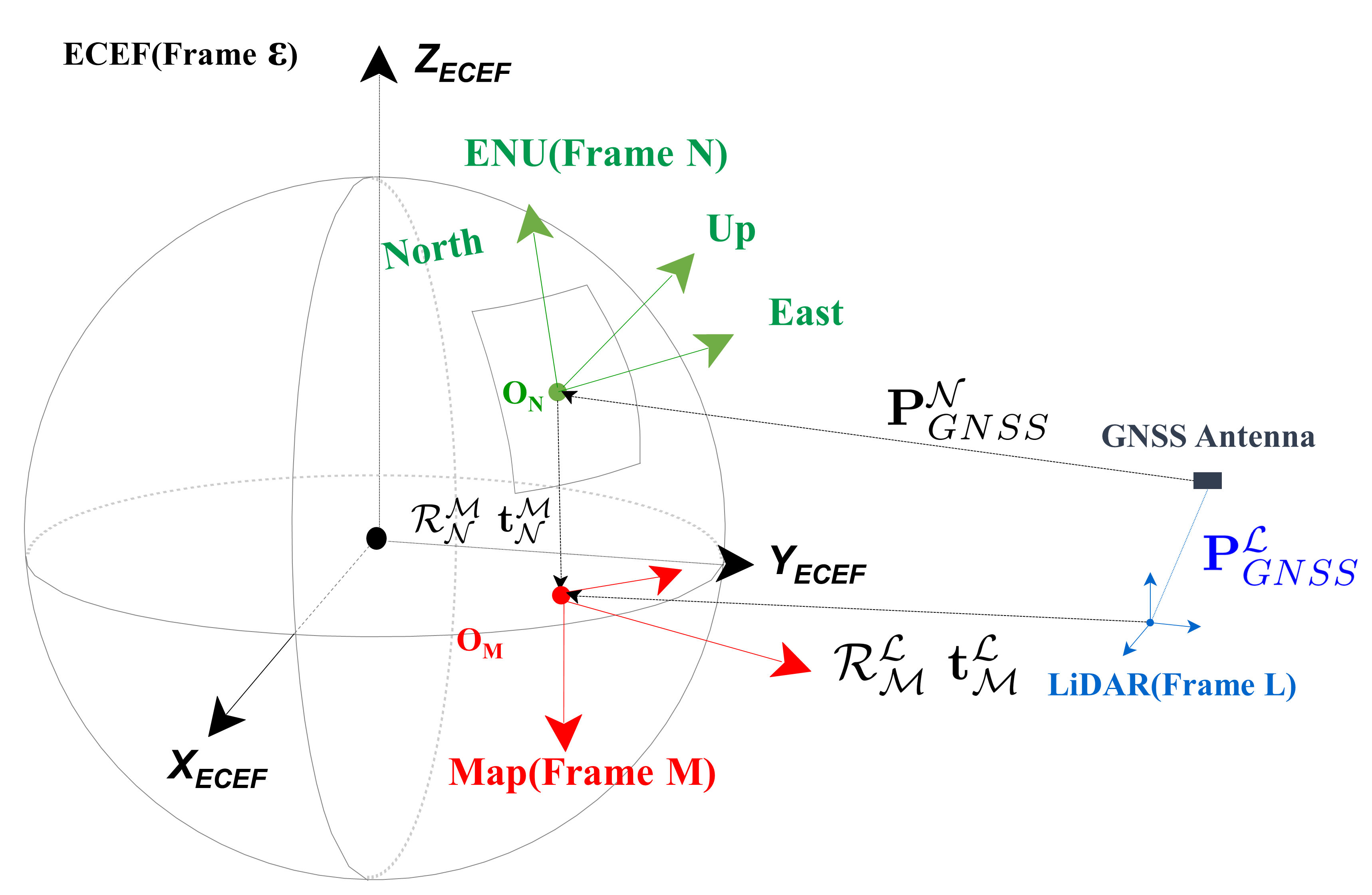
Figure 2: Coordinate Frames

III-B Covariance Estimation of LiDAR-SLAM

In many mainstream LiDAR-SLAM systems, ICP is a key issue which can be solved by many methods to obtain the rotation and translation between two point clouds. After this, the corresponding relations between these two point clouds are obtained, then we use SVD Jacobian model to analyze the covariance of rotation and translation.

III-B1 An explicit analytic solution of ICP using SVD

There are two point sets, {$\mathbf{A}_{i}\}_{i=1}^{n}$ and {$\mathbf{B}_{i}\}_{i=1}^{n}$. Their centers are marked as $\{\mathbf{A}_{c}\}$ and $\{\mathbf{B}_{c}\}$. Both of them can be calculated by Eq.(1).

$$\begin{cases}\mathbf{A}_{c}=\frac{1}{n}\sum_{i=1}^{n}\mathbf{A}_{i}\\ \mathbf{B}_{c}=\frac{1}{n}\sum_{i=1}^{n}\mathbf{B}_{i}\end{cases}$$ (1)

{$\mathbf{M}_{i}\}_{i=1}^{n}$ and {$\mathbf{N}_{i}\}_{i=1}^{n}$ are the normalized coordinates of {$\mathbf{A}_{i}\}_{i=1}^{n}$ and {$\mathbf{B}_{i}\}_{i=1}^{n}$. They can be calculated by Eq.(2).

$$\begin{cases}\mathbf{M}_{i}=\mathbf{A}_{i}-\mathbf{A}_{c}\\ \mathbf{N}_{i}=\mathbf{B}_{i}-\mathbf{B}_{c}\end{cases}$$ (2)

Matrix $\mathbf{W}$ can be calculated by Eq.(3).

$$\mathbf{W}=\sum_{i=1}^{n}\mathbf{N}_{i}\mathbf{M}_{i}^{T}$$ (3)

We apply SVD to $\mathbf{W}$ using Eq.(4). $\mathbf{U}$ and $\mathbf{V}$ are both 3$\times$3 orthonormal matrices. The columns of $\mathbf{U}$ and $\mathbf{V}$ are defined as the left-singular vectors and right-singular vectors of $\mathbf{W}$, respectively. $\mathbf{D}$ is a 3$\times$3 diagonal matrix with the singular values of $\mathbf{W}$.

$$\mathbf{W}=\mathbf{UDV}^{T}$$ (4)

Then the rotation matrix and the translation vector from {$\mathbf{A}_{i}\}_{i=1}^{n}$ to {$\mathbf{B}_{i}\}_{i=1}^{n}$ can be calculated by Eq.(5).

$$\begin{cases}\mathbf{R}_{\mathcal{A}}^{\mathcal{B}}=\mathbf{UV}^{T}\\ \mathbf{t}_{\mathcal{A}}^{\mathcal{B}}=\mathbf{B}_{c}-\mathbf{R}_{\mathcal{A}}^{\mathcal{B}}\mathbf{A}_{c}\end{cases}$$ (5)

III-B2 ICP Error Propagation Model based on SVD Jacobian

The error propagation model of ICP is proposed in this subsection based on SVD Jacobian. According to [43], the Jacobian matrices of $\mathbf{U}$, $\mathbf{D}$ and $\mathbf{V}$ with respect to $\mathbf{W}$ can be calculated by Eq.(6).

$$\begin{cases}\frac{\partial\mathbf{D}_{kk}}{\partial\mathbf{W}_{ij}}=\mathbf{U}_{ik}\mathbf{V}_{jk}\\ \frac{\partial\mathbf{U}}{\partial\mathbf{W}_{ij}}=\mathbf{U\Omega}_{\mathbf{U}}^{ij}\\ \frac{\partial\mathbf{V}}{\partial\mathbf{W}_{ij}}=-\mathbf{V\Omega}_{\mathbf{V}}^{ij}\end{cases}$$ (6)

$\mathbf{\Omega}$${}^{ij}_{\mathbf{U}}$ and $\mathbf{\Omega}$${}^{ij}_{\mathbf{V}}$ are both matrices and their elements $\mathbf{\Omega}$${}^{ij}_{\mathbf{U}_{kl}}$ and $\mathbf{\Omega}$${}^{ij}_{\mathbf{V}_{kl}}$can be caluculated by Eq.(7).

$$\begin{cases}\mathbf{D}_{ll}\mathbf{\Omega}_{\mathbf{U}_{kl}}^{ij}+\mathbf{D}_{kk}\mathbf{\Omega}_{\mathbf{V}_{kl}}^{ij}=\mathbf{U}_{ik}\mathbf{V}_{jl}\\ \mathbf{D}_{kk}\mathbf{\Omega}_{\mathbf{U}_{kl}}^{ij}+\mathbf{D}_{ll}\mathbf{\Omega}_{\mathbf{V}_{kl}}^{ij}=-\mathbf{U}_{il}\mathbf{V}_{jk}\end{cases}$$ (7)

According to Eq.(5), the covariance of $\mathbf{R}_{\mathcal{A}}^{\mathcal{B}}$, marked as $\mathbf{\Lambda_{R^{\mathcal{B}}_{\mathcal{A}}}}$, can be calculated by Eq.(8).

$$\begin{cases}\mathbf{\Lambda_{R^{\mathcal{B}}_{\mathcal{A}}}}=\frac{\partial\mathbf{UV}^{T}}{\partial\mathbf{W}}\mathbf{\Lambda_{W}}\frac{\partial(\mathbf{UV}^{T})^{T}}{\partial\mathbf{W}}\\ \frac{\partial\mathbf{UV}^{T}}{\partial\mathbf{W}_{ij}}=\frac{\partial\mathbf{U}}{\partial\mathbf{W}_{ij}}\mathbf{V}^{T}+\mathbf{U}\frac{\partial\mathbf{V}^{T}}{\partial\mathbf{W}_{ij}}\end{cases}$$ (8)

After $\mathbf{\Lambda_{R^{\mathcal{B}}_{\mathcal{A}}}}$ is obtained, $\mathbf{\Lambda_{t^{\mathcal{B}}_{\mathcal{A}}}}$ can be calculated by Eq.(9).

$$\begin{cases}\mathbf{\Lambda_{t^{\mathcal{B}}_{\mathcal{A}}}}=\mathbf{\Lambda}_{\mathbf{B}_{c}}+\mathbf{\Lambda}_{\mathbf{R}_{\mathcal{A}}^{\mathcal{B}}\mathbf{A}_{c}}\\ \mathbf{\Lambda}_{\mathbf{R}_{\mathcal{A}}^{\mathcal{B}}\mathbf{A}_{c}}=\mathbf{A}_{c}^{T}\mathbf{\Lambda}_{\mathbf{R}_{\mathcal{A}}^{\mathcal{B}}}\mathbf{A}_{c}\end{cases}$$ (9)

The original measurements of {$\mathbf{A}_{i}\}_{i=1}^{n}$ and {$\mathbf{B}_{i}\}_{i=1}^{n}$ are in polar coordinates in the form of one distance and two angles, marked as $\mathbf{d}$ (distance between LiDAR and the measured point), $\bm{\omega}$ (vertical angle) and $\bm{\alpha}$ (horizontal angle). The original measurement error in polar coordinates can be passed to Cartesian coordinates by coordinate transformation so that we can easily obtain $\mathbf{\Lambda_{W}}$ in Eq.(8).

In conclusion, we summarize the ICP error propagation model based on SVD Jacobian in Algorithm 1.

Algorithm 1 ICP Error Propagation Model based on SVD Jacobian

1:Two point sets in polar coordinates $\mathbf{P,Q}$ and their covariance $\mathbf{\Lambda_{P}}$, $\mathbf{\Lambda_{Q}}$; ICP results between $\mathbf{P}$ and $\mathbf{Q}$: $\mathbf{t}_{\mathbf{P}}^{\mathbf{Q}}$, $\mathbf{R}_{\mathbf{P}}^{\mathbf{Q}}$; Corresponding relations between $\mathbf{P}$ and $\mathbf{Q}$: $\mathbf{C}_{\mathbf{PQ}}$;

2:$\mathbf{\Lambda_{t^{\mathbf{Q}}_{\mathbf{P}}}}$, $\mathbf{\Lambda_{R^{\mathbf{Q}}_{\mathbf{P}}}}$;

3:[$\mathbf{A,B}$, $\mathbf{\Lambda_{A}}$, $\mathbf{\Lambda_{B}}$]=Polar2Cart($\mathbf{P,Q}$, $\mathbf{\Lambda_{P}}$, $\mathbf{\Lambda_{Q}}$); //Turn the point sets coordinates and their covariance from polar coordinates to Cartesian coordinates;

4:$\mathbf{t}_{\mathbf{A}}^{\mathbf{B}}$ = $\mathbf{t}_{\mathbf{P}}^{\mathbf{Q}}$, $\mathbf{R}_{\mathbf{A}}^{\mathbf{B}}$ = $\mathbf{R}_{\mathbf{P}}^{\mathbf{Q}}$, $\mathbf{C}_{\mathbf{AB}}$ = $\mathbf{C}_{\mathbf{PQ}}$;

5:Eq.(1), (2), (3), (4) to calculate $\mathbf{U,D,V}$ and $\mathbf{\Lambda_{W}}$;

6:Eq.(6), (7) to calculate the Jacobian matrix of $\mathbf{U,D,V}$ with respect to $\mathbf{W}$;

7:Eq.(8) to calculate $\mathbf{\Lambda_{t^{\mathbf{B}}_{\mathbf{A}}}}$;

8:Eq.(9) to calculate $\mathbf{\Lambda_{\mathbf{R}^{\mathbf{B}}_{\mathbf{A}}}}$;

9:$\mathbf{\Lambda_{t^{\mathbf{Q}}_{\mathbf{P}}}}$ = $\mathbf{\Lambda_{t^{\mathbf{B}}_{\mathbf{A}}}}$ $\mathbf{\Lambda_{\mathbf{R}^{\mathbf{Q}}_{\mathbf{P}}}}$ = $\mathbf{\Lambda_{\mathbf{R}^{\mathbf{B}}_{\mathbf{A}}}}$;

10:return $\mathbf{\Lambda_{t^{\mathbf{Q}}_{\mathbf{P}}}}$, $\mathbf{\Lambda_{R^{\mathbf{Q}}_{\mathbf{P}}}}$;

III-C Single Frequency Precise Point Positioning

In our paper, we choose SF-PPP algorithm to realize PPP for two reasons. One is that single-frequency GNSS receivers are still favored by a large number of users because of its low cost. The other is that the dataset we use only includes single-frequency GNSS data. The basic SF-PPP observation equations are listed in Eq.(10) [44].

$$\begin{split}\begin{cases}\operatorname{Pr}=p_{r}^{s}+c\cdot\left(dt_{r}-dT^{s}\right)+d_{orb}+d_{ion}+d_{trop}\\ \qquad+d_{rel}+\varepsilon(\operatorname{Pr})\\ \Phi_{L}=p_{r}^{s}+c\cdot\left(dt_{r}-dT^{s}\right)+d_{orb}-d_{ion}+d_{trop}\\ \qquad+\lambda_{L}\cdot N_{L}+d_{rel}+d_{pw}+\varepsilon\left(\Phi_{L}\right)\end{cases}\end{split}$$ (10)

$\operatorname{Pr}$ is pseudorange measurement while $\Phi_{L}$ stands for carrier phase range measurement. $p_{r}^{s}$ is the true geometric range between the GNSS receiver and satellite. $c$ means the speed of light. $dt_{r}$ represents the GNSS receiver clock error to be estimated. $dT^{s}$ is the satellite clock error which can be eliminated by precise clock products, and $d_{orb}$ stands for the satellite orbit error eliminated by precise orbit products. $d_{ion}$ is the ionospheric error, mitigated by using Global Ionosphere Maps(GIMs) in our paper. $d_{trop}$ is the tropospheric error, corrected by Saastamoinen model. $d_{rel}$ denotes the relativistic effects and $d_{pw}$ is the phase windup error on the carrier phase measurements. $\lambda_{L}$ is the wavelength of the carrier phase. $N_{L}$ is phase ambiguity. $\varepsilon(\operatorname{Pr})$ is pseudorange measurement noise and $\varepsilon\left(\Phi_{L}\right)$ means carrier phase range measurement noise. It is interesting to note here that Difference Code Bias (DCB) of P2/P1 and P1/C1 need to be corrected by IGS products for Ionosphere [45].

For every epoch and every GNSS satellite, we obtain Eq.(10), then the equations of all satellites in one epoch are linearized and marked as Eq.(11). $\mathbf{Z}_{C}$ and $\mathbf{Z}_{P}$ respectively represent the carrier phase range and pseudorange measurements of all GNSS satellites. $\mathbf{B}_{C}$ and $\mathbf{B}_{P}$ are the corresponding Jacobian matrices.

$$\begin{split}\left[\begin{smallmatrix}\mathbf{Z}_{C}\\ \mathbf{Z}_{P}\end{smallmatrix}\right]&=\left[\begin{smallmatrix}\mathbf{B}_{C}\\ \mathbf{B}_{P}\end{smallmatrix}\right]\left[\begin{smallmatrix}\mathbf{X}\\ c\cdot dtr\\ \mathbf{N}_{L}\end{smallmatrix}\right]+\left[\begin{smallmatrix}\mathbf{\Delta}_{C}\\ \mathbf{\Delta}_{P}\end{smallmatrix}\right]\end{split}$$ (11)

Since the pseudorange’s variance $\mathbf{D(\Delta}_{P})$ is different from the carrier phase’s variance $\mathbf{D(\Delta}_{C})$, the weights of pseudorange and carrier phase are different. If there are n satellites observed in one epoch, then $\mathbf{V}$ is the residual vector of this epoch, which can be calculated by Eq.(12).

$$\begin{split}\mathbf{V}&=\left[\begin{smallmatrix}\mathbf{Z}_{C}\\ \mathbf{Z}_{P}\end{smallmatrix}\right]-\left[\begin{smallmatrix}\mathbf{B}_{C}\\ \mathbf{B}_{P}\end{smallmatrix}\right]\left[\begin{smallmatrix}\mathbf{\tilde{X}}\\ c\cdot\tilde{dtr}\\ \mathbf{\tilde{N}}_{L}\end{smallmatrix}\right]=\mathbf{Z}-\mathbf{B}\left[\begin{smallmatrix}\mathbf{\tilde{X}}\\ c\cdot\tilde{dtr}\\ \mathbf{\tilde{N}}_{L}\end{smallmatrix}\right]\end{split}$$ (12)

SF-PPP covariance, $cov(\mathbf{\tilde{X}})$, is the first three rows and first three columns of Eq.(13), $cov(\mathbf{\tilde{X}},c\cdot\tilde{dtr},\mathbf{\tilde{N}}_{L})_{(1:3,1:3)}$.

$$\begin{split}cov(\mathbf{\tilde{X}},c\cdot\tilde{dtr},\mathbf{\tilde{N}}_{L})&=\frac{\mathbf{V}^{\mathrm{T}}\mathbf{P}\mathbf{V}}{n-4}\left(\mathbf{B}^{\mathrm{T}}\mathbf{P}\mathbf{B}\right)^{-1}=m_{0}^{2}\cdot\mathbf{Q}_{\mathrm{x}}\\ P&=\left[\begin{smallmatrix}\mathbf{D(\Delta}_{C})&0\\ 0&\mathbf{D(\Delta}_{C})\\ \end{smallmatrix}\right]^{-1}\end{split}$$ (13)

The diagonal of $\mathbf{Q}_{\mathrm{x}}$ constitutes the DOP (Dilution of Precision) values which reflect the spatial structure of the satellites.

III-D Ground Truth Calculation of LiDAR-SLAM Positioning Covariance Assisted with GNSS

Based on GNSS positioning covariance introduced above, we calculate the ground truth of LiDAR-SLAM positioning covariance in this subsection. There are three positioning results in Fig. 3: the red $X_{gt}$ is ground truth, the blue $X_{G}$ is GNSS positioning result and the green $X_{L}$ is LiDAR-SLAM positioning result. $X_{G}$ and $X_{L}$ are independent of each other and both satisfy the Gaussian distribution. As such, if using linear weighted average algorithm to fuse $X_{G}$ and $X_{L}$, then the optimal estimation under linear weighted criterion, $X_{opt}$, must satisfy $X_{opt}X_{gt}\bot X_{G}X_{L}$. Through this vertical relationship, $X_{opt}$ can be calculated by Eq.(14).

$$\begin{split}\overrightarrow{X_{G}X_{opt}}&=\frac{\overrightarrow{X_{G}X_{gt}}\cdot\overrightarrow{X_{G}X_{L}}}{|\overrightarrow{X_{G}X_{L}}|}\cdot\frac{\overrightarrow{X_{G}X_{L}}}{|\overrightarrow{X_{G}X_{L}}|}\\ \Rightarrow X_{opt}&=\frac{\overrightarrow{X_{G}X_{gt}}\cdot\overrightarrow{X_{G}X_{L}}}{|\overrightarrow{X_{G}X_{L}}|}\cdot\frac{\overrightarrow{X_{G}X_{L}}}{|\overrightarrow{X_{G}X_{L}}|}+X_{G}\end{split}$$ (14)

After obtaining $X_{opt}$, the ground truth of LiDAR-SLAM positioning covariance can be calculated by Eq.(15).

$$Cov\left(X_{L}\right)=\frac{|\overrightarrow{X_{opt}X_{L}}|}{|\overrightarrow{X_{G}X_{opt}}|}Cov\left(X_{G}\right)$$ (15)

Eq.(15) is proved as follows. Since $X_{L}$ and $X_{G}$ are random variables subject to Gaussian distribution, we mark them as $X_{L}\sim N(u_{X_{L}},Cov(X_{L}))$ and $X_{G}\sim N(u_{X_{G}},Cov(X_{G}))$. $X_{lwa}$, the linear weighted average of $X_{L}$ and $X_{G}$, equals to $\lambda X_{L}+(1-\lambda)X_{G}$ and is subject to Eq.(16).

$$X_{lwa}\sim N(\lambda u_{X_{L}}+(1-\lambda)u_{X_{G}},\lambda^{2}Cov(X_{L})+(1-\lambda)^{2}Cov(X_{G}))$$ (16)

In addition, under linear weighted criterion, the weight is inversely proportional to the distance, so $\lambda$ must satisfy Eq.(17).

$$\lambda|\overrightarrow{X_{G}X_{lwa}}|=(1-\lambda)|\overrightarrow{X_{lwa}X_{L}}|$$ (17)

It is noted that the optimal value of $X_{lwa}$ is $X_{opt}$, which can be derived from minimizing $Cov(X_{lwa})$, as Eq.(18) shows.

$$\begin{split}&\underset{\lambda}{\operatorname{\mathbf{argmin}}}\left(\lambda^{2}Cov(X_{L})+(1-\lambda)^{2}Cov(X_{G})\right)\\ \Rightarrow&\underset{\lambda}{\operatorname{\mathbf{argmin}}}\left((Cov(X_{L})+Cov(X_{G}))\lambda^{2}-2Cov(X_{G})\lambda+Cov(X_{G})\right)\\ \Rightarrow&((Cov(X_{L})+Cov(X_{G}))\lambda=Cov(X_{G})\\ \end{split}$$ (18)

Where $\lambda$ can be eliminated by combining Eq.(17) and Eq.(18) to prove Eq.(15).

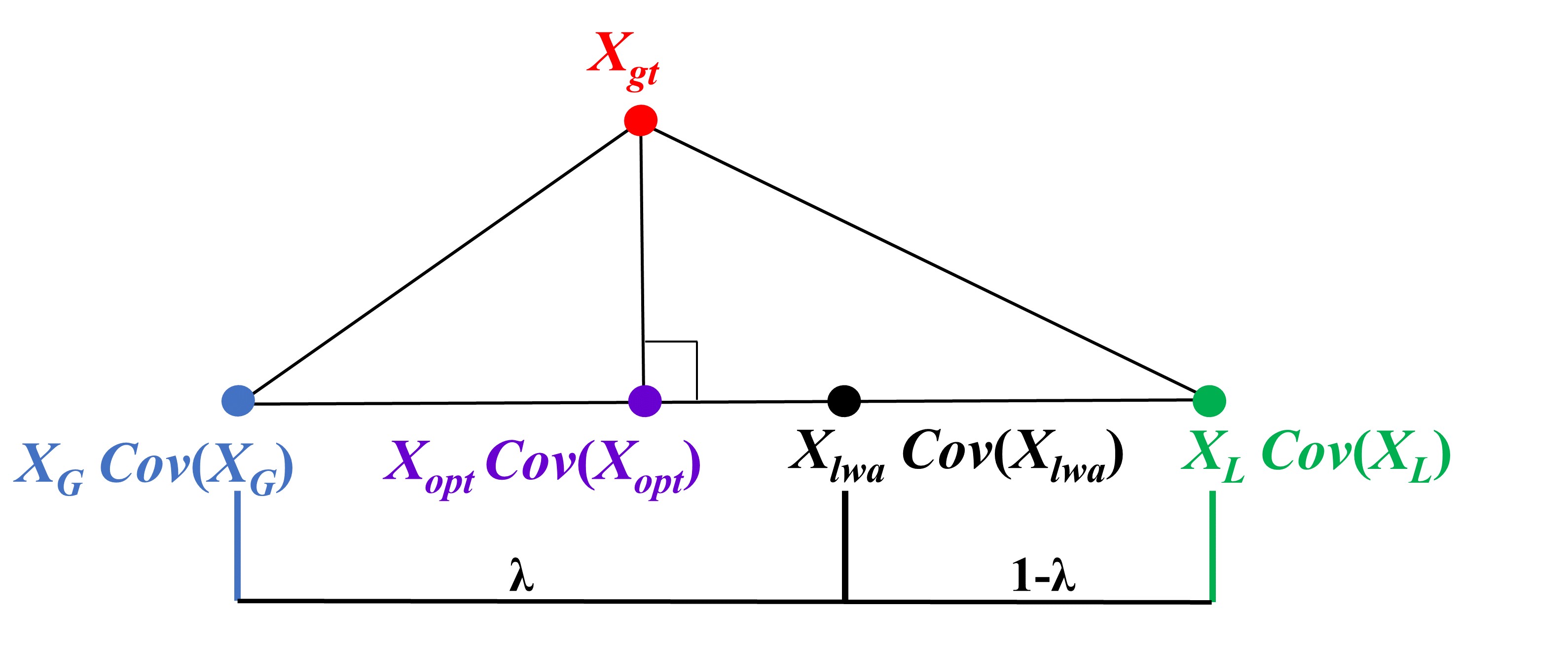
Figure 3: Ground Truth Calculation of LiDAR-SLAM Position Covariance Assisted with GNSS

III-E LiDAR-SLAM Assisted GNSS RAIM Algorithm

In urban canyon environment, GNSS is seriously affected by the multipath and NLOS. GNSS RAIM algorithm is normally adopted to detect the outliers of satellite observations. But simultaneous presence of multiple outliers might underperform the existing GNSS RAIM algorithm. In this subsection, LiDAR-SLAM assisted GNSS RAIM algorithm is proposed, the main flow of which is shown in Algorithm 2. Our RAIM Algorithm only uses pseudorange observations, so when the pseudorange of one satellite is detected as an outlier, the phase observation of this observation is also considered an outlier.

Algorithm 2 LiDAR-SLAM assisted GNSS RAIM algorithm

Input: LiDAR-SLAM positioning result $X_{L}$, SPP result from ublox receiver $X_{G}$;
  Output: GNSS Satellite Inliers;

1:while New GNSS Observation Comes do

2:     $X_{F}$ = SPP-LOAM($X_{L}$,$X_{G}$); //Fuse $X_{L}$ and $X_{G}$ by SPP-LOAM to get $X_{F}$ as fusion result;

3:     $dtr$ = $dtr$Est($X_{F}$, Pseudoranges); //Receiver clock error estimation;

4:     V=ResCal($X_{F}$, Pseudoranges, $dtr$); //Calculate pseudorange residuals by using Eq.(10);

5:     [mean, std] = CalMeanStd(V); //For every GNSS satellite in this epoch, calculate the mean and standard deviation of its pseudorange residuals;

6:     if —V[j] - mean— $\leq$ $\alpha\cdot$std (//$\alpha$ is an input coefficient) then

7:         Set GNSS satellite j observations as inlier;

8:     else

9:         Set GNSS satellite j observations as outlier;

10:     end if

11:end while

12:return GNSS Satellite Inliers;

III-F Pose Graph Model

In this subsection, we give the pose graph model in the form of factor graph (see Fig. 4). Then the specific optimization functions will be listed.

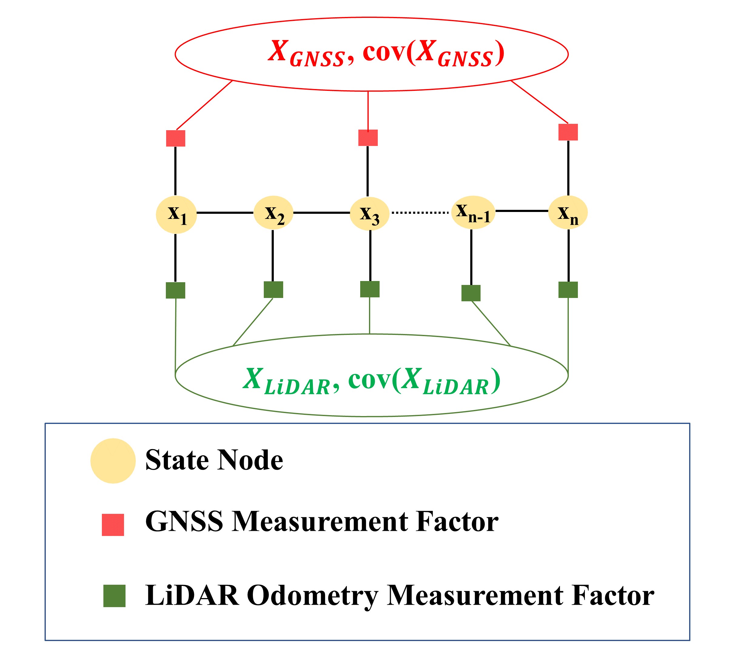
Figure 4: Factor Graph of the Backend

GNSS positioning results reflect the position of the GNSS antenna phase center which is represented as $\mathbf{P}_{G}^{\mathcal{N}}$ in Frame $\mathcal{N}$. And the GNSS antenna phase center in Frame $\mathcal{L}$, also known as the extrinsic parameter, is represented as $\mathbf{P}_{G}^{\mathcal{L}}$. Other notations can be found in Table I. According to the coordinate transformation, we obtain the equation Eq.(19).

$$\mathbf{R}_{\mathcal{N}}^{\mathcal{M}}\mathbf{P}_{G}^{\mathcal{N}}+\mathbf{t}_{\mathcal{N}}^{\mathcal{M}}=\mathbf{R}_{\mathcal{L}}^{\mathcal{M}}\mathbf{P}_{G}^{\mathcal{L}}+\mathbf{t}_{\mathcal{L}}^{\mathcal{M}}$$ (19)

According to Eq.(19), the residual equation Eq.(20) is obtained:

$$\begin{split}\begin{aligned} \mathbf{r}_{1}&=\mathbf{r}_{GNSS_{-}\text{LiDAR}}\\ &=\mathbf{R}_{\mathcal{M}}^{\mathcal{N}}\left(\mathbf{R}_{\mathcal{L}}^{\mathcal{M}}\mathbf{P}_{G}^{\mathcal{L}}+\mathbf{t}_{\mathcal{L}}^{\mathcal{M}}-\mathbf{t}_{\mathcal{N}}^{\mathcal{M}}\right)-\mathbf{P}_{G}^{\mathcal{N}}\end{aligned}\end{split}$$ (20)

And LiDAR-SLAM outputs a 6DoF pose with a certain frequency. This paper defines LiDAR-SLAM output as prior information. The prior residual is listed in Eq.(21) where $i$ and $j$ are two epochs when LiDAR observations are obtained.

$$\begin{array}[]{c}\mathbf{r}_{2}=\mathbf{r}_{LiDAR_{-}\text{prior}}\!=\!\end{array}\left[\begin{array}[]{c}\mathcal{R}^{\mathcal{L}}_{\mathcal{M},i}\left(\mathbf{t}_{\mathcal{L},j}^{\mathcal{M}}-\mathbf{t}_{\mathcal{L},i}^{\mathcal{M}}\right)\\ \log\left(\mathcal{R}^{\mathcal{L}}_{\mathcal{M},i}\mathcal{R}_{\mathcal{L},j}^{\mathcal{M}}\right)^{\vee}\end{array}\right]$$ (21)

The optimization function Eq.(22) is obtained after combining Eq.(20) and Eq.(21).

$$\underset{\mathbf{R}_{\mathcal{N}}^{\mathcal{M}},\mathbf{t}_{\mathcal{N}}^{\mathcal{M}},\mathbf{R}_{\mathcal{L}}^{\mathcal{M}},\mathbf{t}_{\mathcal{L}}^{\mathcal{M}},\mathcal{P}_{G}^{\mathcal{L}}}{\operatorname{\mathbf{argmin}}}\left(\left\|\mathbf{r}_{1}\right\|_{\Sigma_{1}}^{2}+\left\|\mathbf{r}_{2}\right\|_{\Sigma_{2}}^{2}\right)$$ (22)

The specific optimization functions for every observation epoch are listed in Eq.(23). Then we use Levenberg-Marquard algorithm to solve the cost function where a 15DoF variable needs to be optimized. Its first six dimensions determine the coordinate transformation between Frame $\mathcal{N}$ and Frame $\mathcal{M}$. The next six dimensions determine the pose of experimental vehicle. The last three dimensions are the extrinsic parameters.

$$\begin{split}\left[\begin{smallmatrix}\mathbf{r}_{1}\\ \mathbf{r}_{2}\\ \end{smallmatrix}\right]&=\left[\begin{smallmatrix}\mathcal{R}_{\mathcal{M}}^{\mathcal{N}}\left(\mathcal{R}_{\mathcal{L}}^{\mathcal{M}}P_{G}^{\mathcal{L}}+\mathbf{t}_{\mathcal{L}}^{\mathcal{M}}-\mathbf{t}_{\mathcal{N}}^{\mathcal{M}}\right)^{\wedge}&\bm{0_{3\times 3}}\\ -\mathcal{R}_{\mathcal{M}}^{\mathcal{N}}&\bm{0_{3\times 3}}\\ \mathcal{R}_{\mathcal{M}}^{\operatorname{\mathcal{N}}}\left(-\mathcal{R}_{\mathcal{L}}^{\mathcal{M}}P_{G}^{\mathcal{L}}\right)^{\wedge}&\mathcal{R}_{\mathcal{M}}^{\mathcal{L}}\\ \mathcal{R}_{\mathcal{M}}^{\mathcal{N}}&\mathcal{R}_{\mathcal{M}}^{\mathcal{L}}\\ \mathcal{R}_{\mathcal{M}}^{\mathcal{N}}\mathcal{R}_{\mathcal{L}}^{\mathcal{M}}&\bm{0_{3\times 3}}\end{smallmatrix}\right]^{T}\left[\begin{smallmatrix}\delta\theta_{\mathcal{N}}^{\mathcal{M}}\\ \delta\mathbf{t}_{\mathcal{N}}^{\mathcal{M}}\\ \delta\theta_{\mathcal{L}}^{\mathcal{M}}\\ \delta\mathbf{t}_{\mathcal{L}}^{\mathcal{M}}\\ \delta\mathcal{P}_{G}^{\mathcal{L}}\\ \end{smallmatrix}\right]\end{split}$$ (23)

All the data was collected and synchronized using the robot operation system (ROS). But these two kinds of observations are not obtained at the same moment. In this case, we use linear extrapolation to obtain a virtual LiDAR observation which can be fused with GNSS.

IV Experiment and analysis

IV-A Experiment Setup

Our experiment used UrbanNav Dataset [41], an open dataset collected by Hong Kong Polytechnic University. In this dataset, a single frequency GNSS receiver, ublox M8T, was used to collect GNSS measurements (only two systems, GPS and Beidou, were collected). The 3D LiDAR (Velodyne 32) was employed to collect 3D point clouds. In addition, the NovAtel SPAN-CPT, an RTK/INS integrated navigation system, was used to provide the ground truth of positioning.

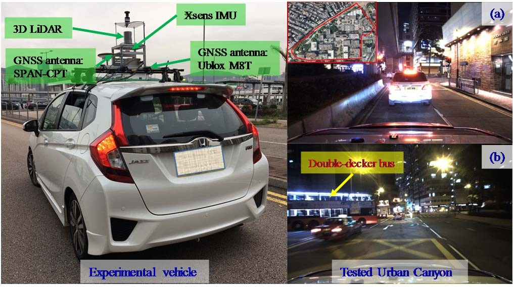
Figure 5: Experimental Vehicle and the Tested Scenario [41]

Fig. 5-(a) shows that the dataset was collected in an urban canyon environment, which is challenging for GNSS. And Fig. 5-(b) shows that there were many dynamic objects such as cars when the dataset was collected, which is challenging for LiDAR-SLAM.

IV-B LiDAR-SLAM Positioning Covariance Estimation Results

The estimated LiDAR-SLAM positioning covariance is in Frame $\mathcal{M}$ and we use Eq.(24) to turn it into Frame $\mathcal{E}$.

$$\begin{cases}Cov(X_{L}^{\mathcal{N}})=\mathbf{R}_{\mathcal{M}}^{\mathcal{N}}Cov(X_{L}^{\mathcal{M}})\mathbf{R}_{\mathcal{N}}^{\mathcal{M}}\\ Cov(X_{L}^{\mathcal{E}})=\mathbf{R}_{\mathcal{N}}^{\mathcal{E}}Cov(X_{L}^{\mathcal{N}})\mathbf{R}_{\mathcal{E}}^{\mathcal{N}}\end{cases}$$ (24)

$\mathbf{R}_{\mathcal{M}}^{\mathcal{N}}$ is estimated from Eq.(24). $B$ and $L$ in Eq.(24) respectively represent the longitude and latitude of the current LiDAR-SLAM positioning results.

$$\mathbf{R}_{\mathcal{N}}^{\mathcal{E}}=\left[\begin{array}[]{ccc}-\sin B\cos L&-\sin B\sin L&\cos B\\ -\sin L&\cos B&0\\ \cos B\cos L&\cos B\sin L&\sin B\end{array}\right]$$ (25)

The LiDAR-SLAM positioning covariance estimation results are shown in Fig. 6, in which the black is the ground truth trajectory, the blue is the GNSS trajectory, and the red is the LiDAR-SLAM trajectory. The red ellipse in the upper part of Fig. 6 represents the LiDAR-SLAM covariance ground truth calculated by Eq.(15). The red ellipse in the bottom part of Fig. 6 shows the estimated LiDAR-SLAM covariance calculated by Eq.(9).

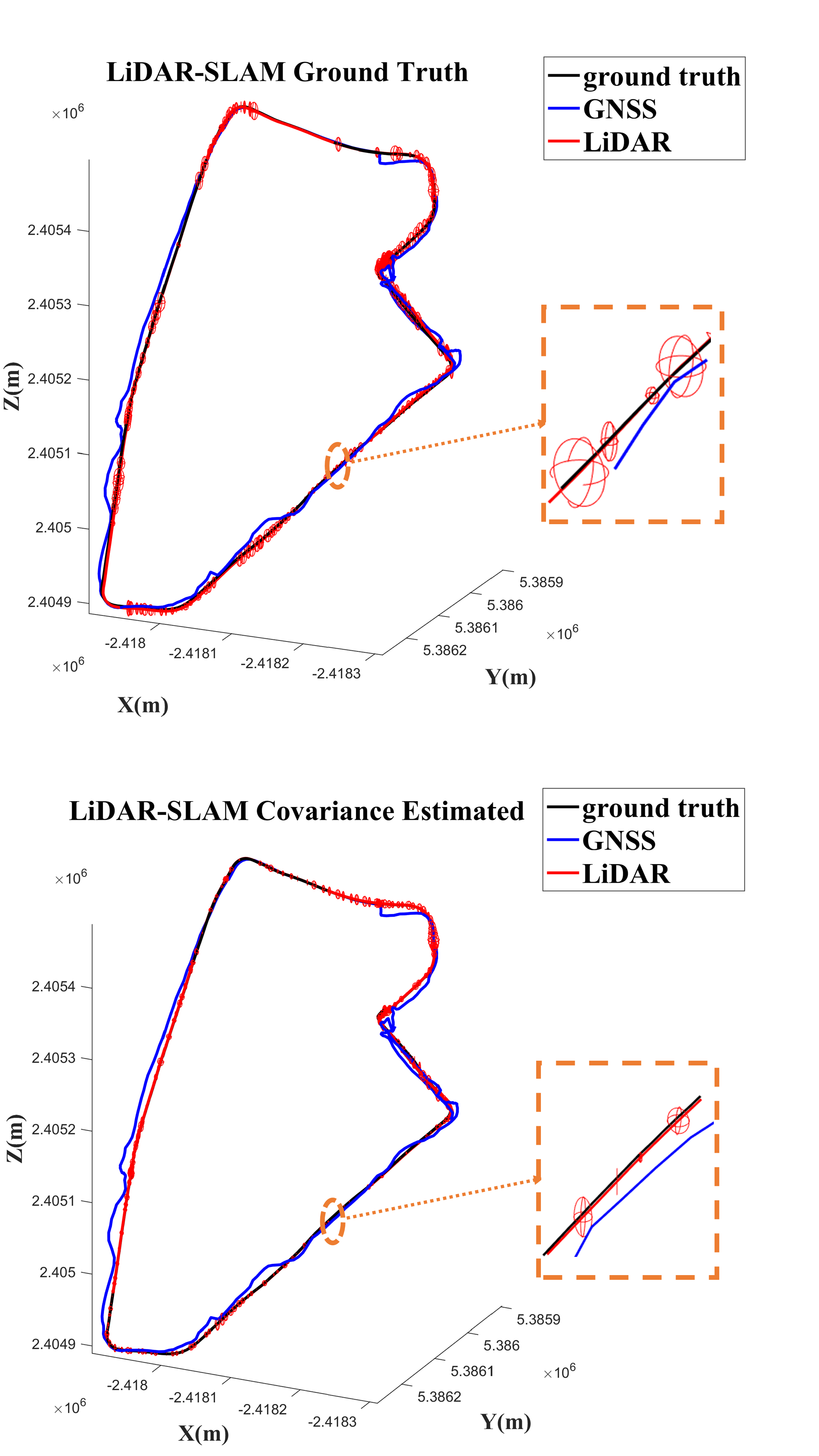
Figure 6: LiDAR-SLAM Covariance Results

In Table II, six groups of values, each composed of the mean and standard deviation, are displayed to represent the difference between the ground truth and estimated LiDAR-SLAM covariance. The means and the standard deviations fall within the range of 0.36m² and 0.54m² respectively, which are relatively small differences comparing to the positioning error.

TABLE II: The Difference Between the Ground Truth and the Estimated Value of LiDAR-SLAM Covariance

	$\Delta$CovX	$\Delta$CovY	$\Delta$CovZ	$\Delta$CovXY	$\Delta$CovYZ	$\Delta$CovZX
Mean($m^{2}$)	0.2365	0.3519	0.2125	0.2831	0.2716	0.2125
Std($m^{2}$)	0.4785	0.5320	0.3575	0.4824	0.4286	0.3575

IV-C LiDAR-SLAM Assisted GNSS RAIM Performance

In this subsection, we will compare the SF-PPP performance before and after using RAIM (Algorithm 2).

When the coefficient $\alpha$ in Algorithm 2 is larger, the effect of RAIM gets smaller. Before using RAIM, the SF-PPP in urban canyon environment has low reliability, as the green points shown in Fig. 7. When the coefficient $\alpha$ gets smaller, the remaining number of positioning results decreases. Different $\alpha$ values have been tried, and finally, $\alpha=2$ is chosen considering the availability and reliability.

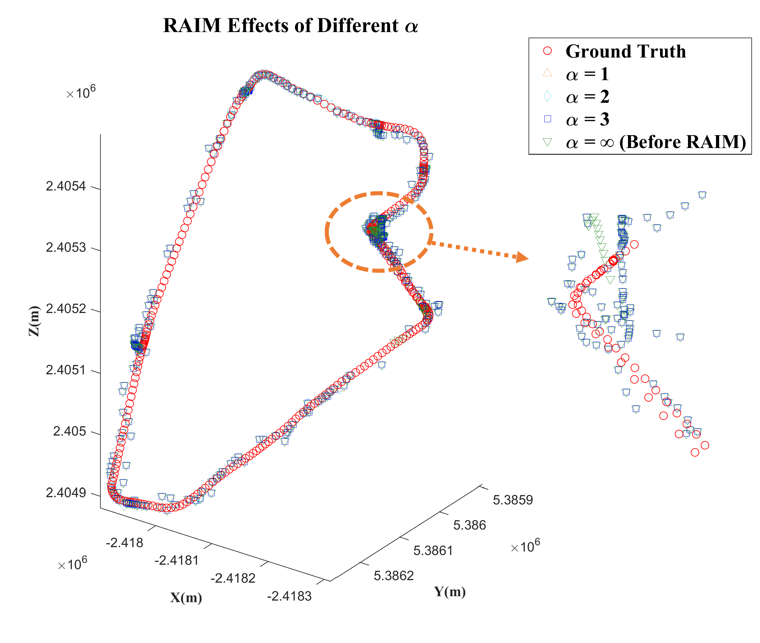
Figure 7: RAIM Effects of Different $\alpha$

The error of PPP (when $\alpha=2$) is plotted in Fig. 8. We find that the availability and accuracy of PPP are much higher between 270 to 390 seconds according to Fig. 8. This is due to better GNSS observation conditions where there are fewer buildings.

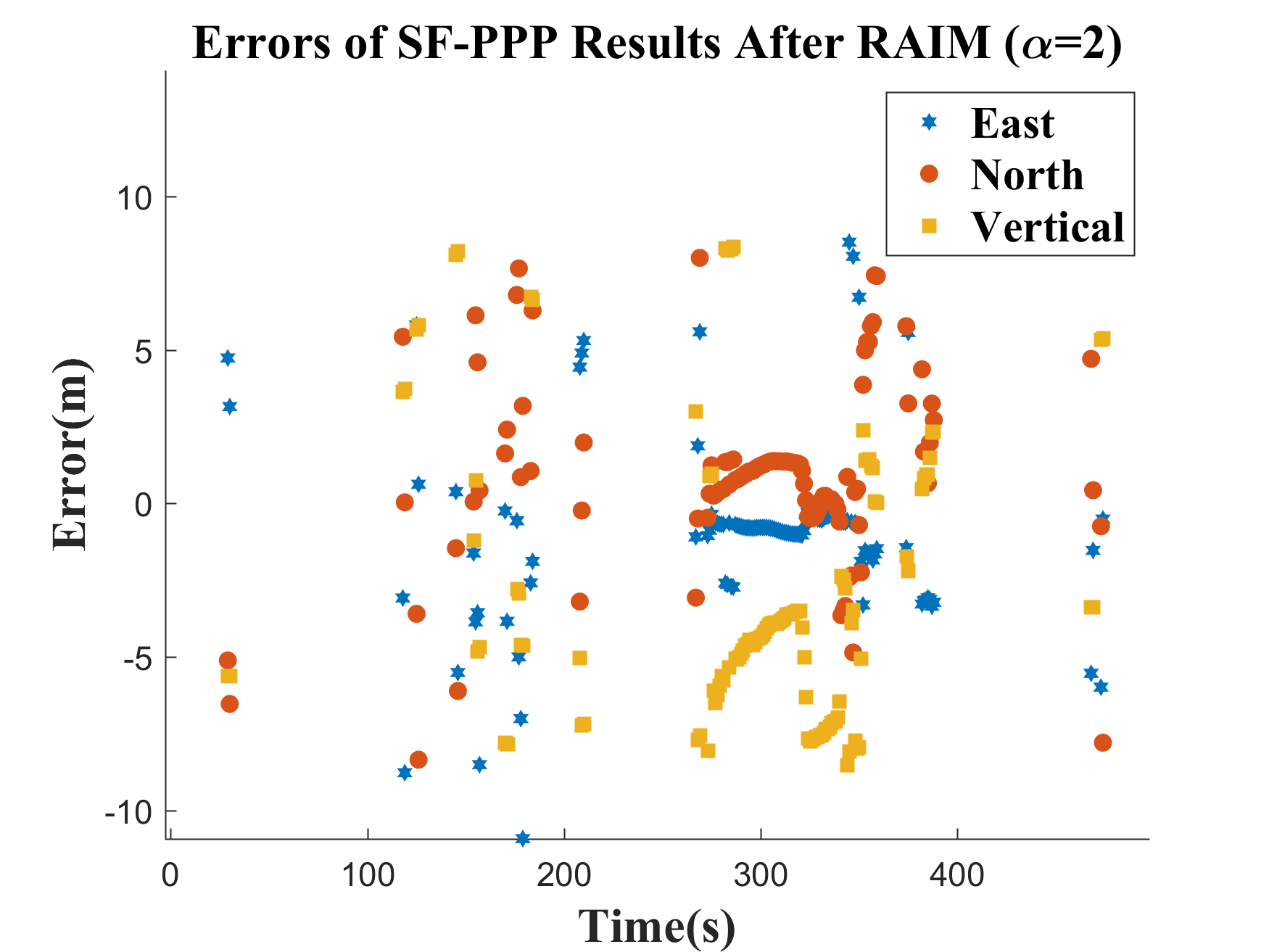
Figure 8: Errors of SF-PPP Results After RAIM

IV-D P³-LOAM Performance

In order to prove the validity of P³-LOAM, several different positioning schemes were compared on UrbanNav. Specific statistical results are in Table III. The column of ‘LeGO-LOAM’ represents LiDAR-SLAM’s results in local coordinates. ‘LeGO-LOAM’ is an open-source software widely used as a benchmark. The column of ‘Hsu et al.’ represents the GNSS and LiDAR-SLAM fusion results reported in [41]. The column of ‘SPP’ represents the GNSS results processed by SPP. The column of ‘PPP’ represents the GNSS results processed by SF-PPP with LiDAR-SLAM assisted RAIM algorithm. The results of ‘PPP’ are shown in Fig. 8. ‘SPP’ and ‘PPP’ are both from RTKLIB, a piece of software often used for GNSS research. The column of ‘SPP-LOAM’ represents the SPP and LiDAR-SLAM fusion results. The column of ‘P³-LOAM’ represents the SF-PPP and LiDAR-SLAM fusion results.

The first four rows of Table III represent error indicators. We use $X$ to represent the ground truth and $\tilde{X}$ to represent the estimated results. The ‘MAE’ is short for ‘Mean Absolute Error’. It can be calculated by Eq.(26).

$$\operatorname{MAE}(\mathrm{\tilde{X}},\mathrm{X})=\frac{1}{\mathrm{m}}\sum_{i=1}^{\mathrm{m}}\left|\mathrm{\tilde{X}}^{(\mathrm{i})}-\mathrm{X}^{(\mathrm{i})}\right|$$ (26)

The ‘RMSE’ is short for ‘Root Mean Square Error’. It can be calculated by Eq.(27).

$$\operatorname{RMSE}(\mathrm{\tilde{X}},\mathrm{X})=\frac{1}{\mathrm{m}}\sum_{i=1}^{\mathrm{m}}\left(\mathrm{\tilde{X}}^{(\mathrm{i})}-\mathrm{X}^{(\mathrm{i})}\right)^{2}$$ (27)

The ‘Max’ represents the max error. The ‘Std’ is short for ‘Standard Deviation’ and represents the standard deviation of error which can be calculated by Eq.(28).

$$\operatorname{Std}=\sqrt{\frac{1}{m}\sum_{i=1}^{m}\left(\left|\mathrm{\tilde{X}}^{(\mathrm{i})}-\mathrm{X}^{(\mathrm{i})}\right|-\operatorname{MAE}\right)^{2}}$$ (28)

The ‘Scale’ row in Table III represents the ability of algorithms to calculate global coordinates.

The ‘Availability’ is calculated by dividing positioning result numbers by observation numbers.

TABLE III: GNSS and LiDAR-SLAM Fusion Results

	LeGO- LOAM [7]	Hsu et al. [41]	SPP	PPP	SPP-LOAM	P3-LOAM
MAE(m)	4.28	4.60	21.18	5.92	20.71	3.44
RMSE(m)	4.50	-∗	27.56	6.17	23.37	3.72
Max(m)	8.27	16.46	88.04	8.95	36.97	7.44
Std(m)	1.40	3.33	17.64	1.73	7.55	1.43
Scale	Local	Global	Global	Global	Global	Global
Availability	$100\%$	$100\%$	$100\%$	$21.4\%$	$100\%$	100%

• The ‘-’ means the result was not reported.

The results in Table III show that P³-LOAM performs best in almost every indicator except in the ‘Std’ where LeGO-LOAM and P³-LOAM have the same level of performance. We analyze that the errors of LeGO-LOAM are larger but more concentrated since SLAM has the property of error accumulation.

Fig. 9-(a) shows all the results plotted on Google Earth. It is evident that the scene is challenging for GNSS. Especially in Fig. 9-(b), (d), (e), where the tall buildings exert negative effects on satellite signals, so SPP and SPP-LOAM cannot perform well here whereas P³-LOAM still provides reliable results. In contrast, the scene in Fig. 9-(c) is friendly to GNSS, so all the results here are close to the ground truth and the PPP results here are more available than in any other parts. Fig. 10 displays the number of available satellites to account for the impact of the scene on GNSS. We can see that Fig. 10-(b) and Fig. 10-(e) have fewer satellites observed than the others, leading to the unsatisfactory GNSS results in these parts. Fig. 10-(c) and Fig. 10-(d) both have adequate satellites, but the performance in Fig. 10-(d) is severely degraded by the multipath effect or NLOS caused by the tall buildings.

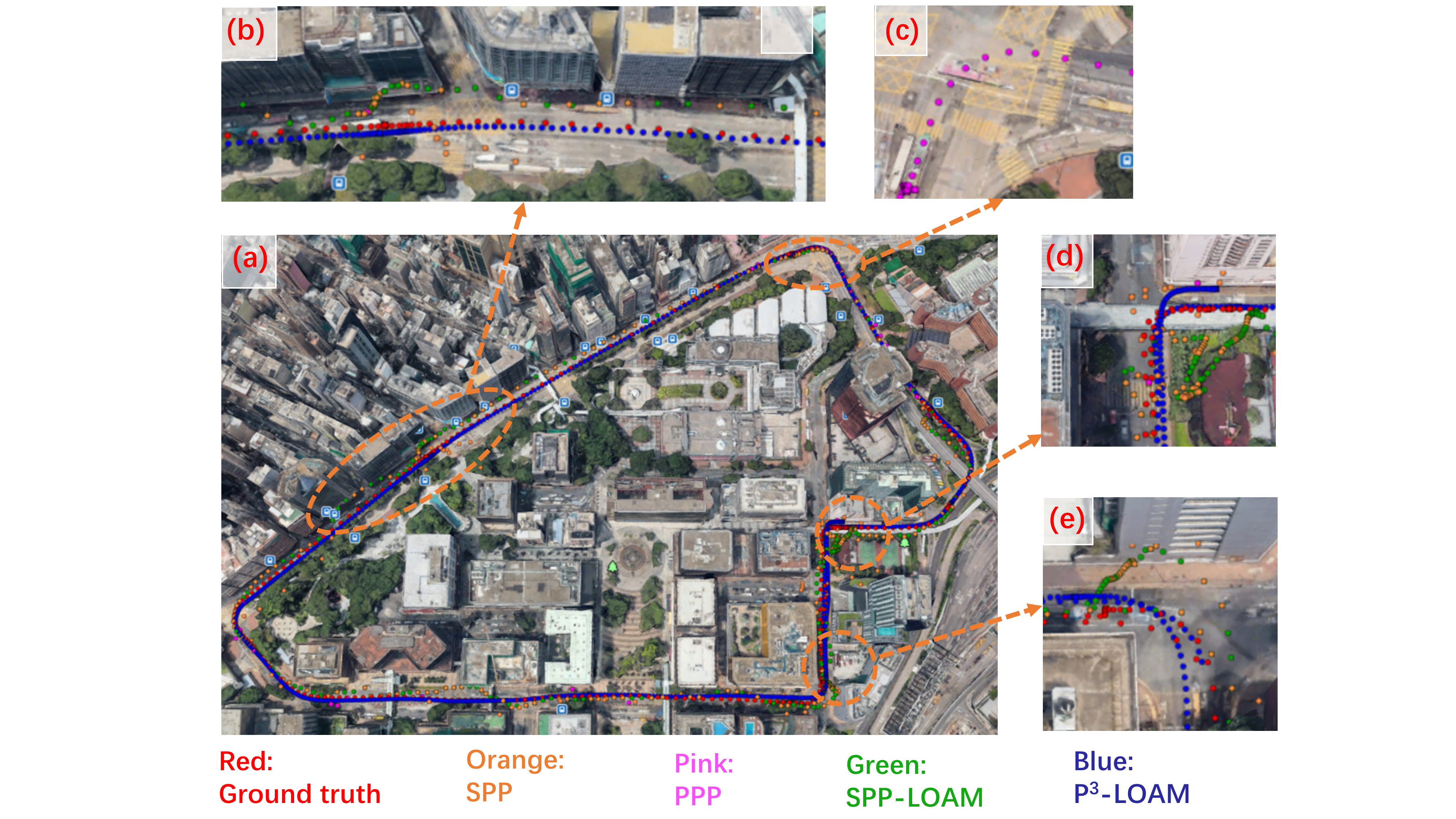
Figure 9: All the Positioning Results on Google Earth

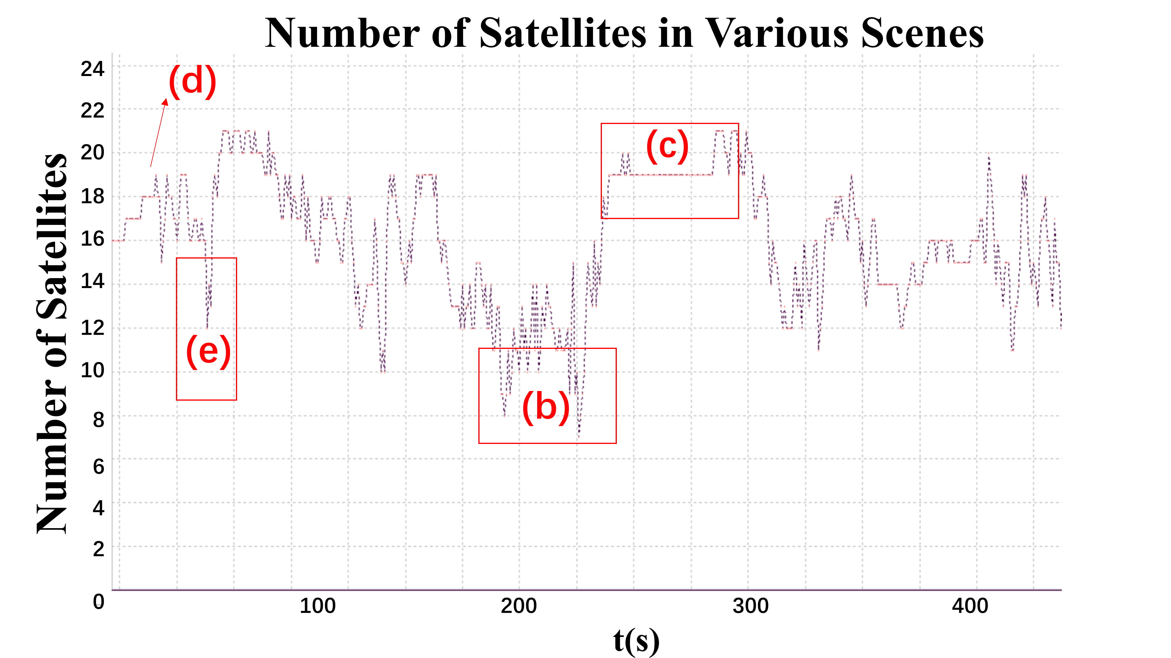
Figure 10: Number of Satellites

The availability of ‘LeGO-LOAM’, ‘SPP’, ‘SPP-LOAM’ and ‘P³-LOAM’ is all 100% which indicates the continuity of algorithms. To compare the availability of these four methods, we further analyze the Cumulative Distribution Function(CDF) of their errors in Fig. 11. If we define the availability as the error under an exact level, such as 5 meters, the availability of ‘SPP’ and ‘SPP-LOAM’ will be much lower than ‘P³-LOAM’ and ‘LeGO-LOAM’. The errors in the east, north and vertical components are also plotted in Fig. 12. It is obvious that ‘P³-LOAM’ performs best when considering accuracy, availability, and the ability to obtain global coordinates.

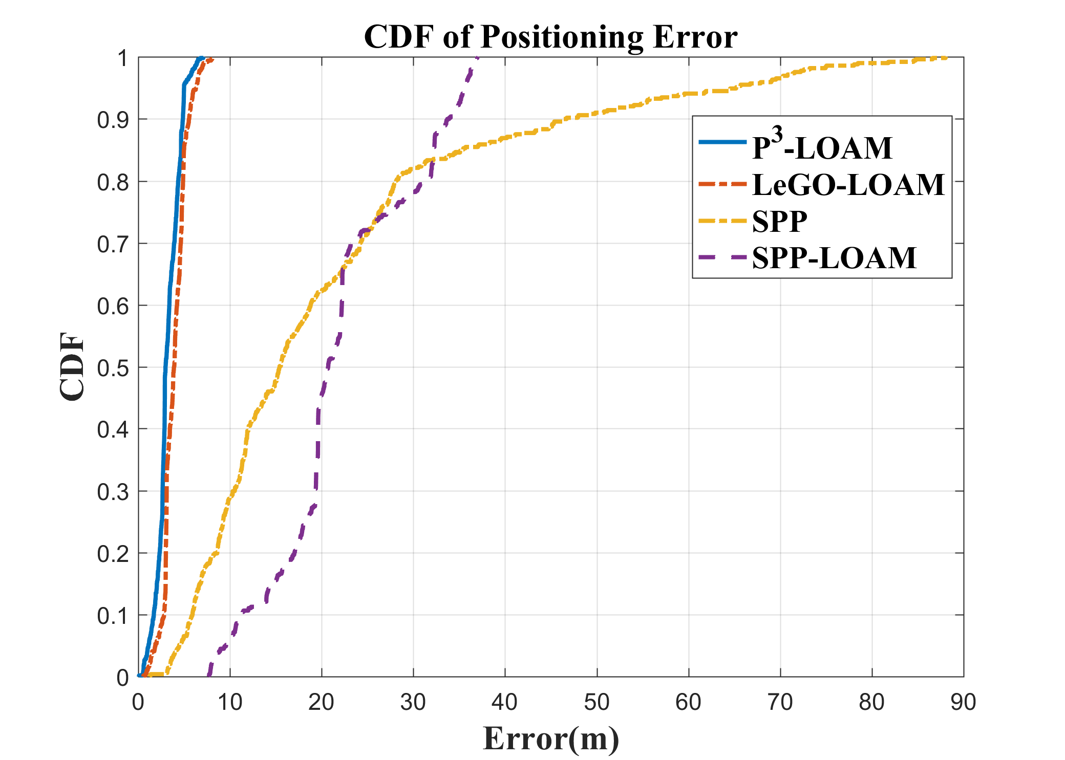
Figure 11: CDF of Positioning Error

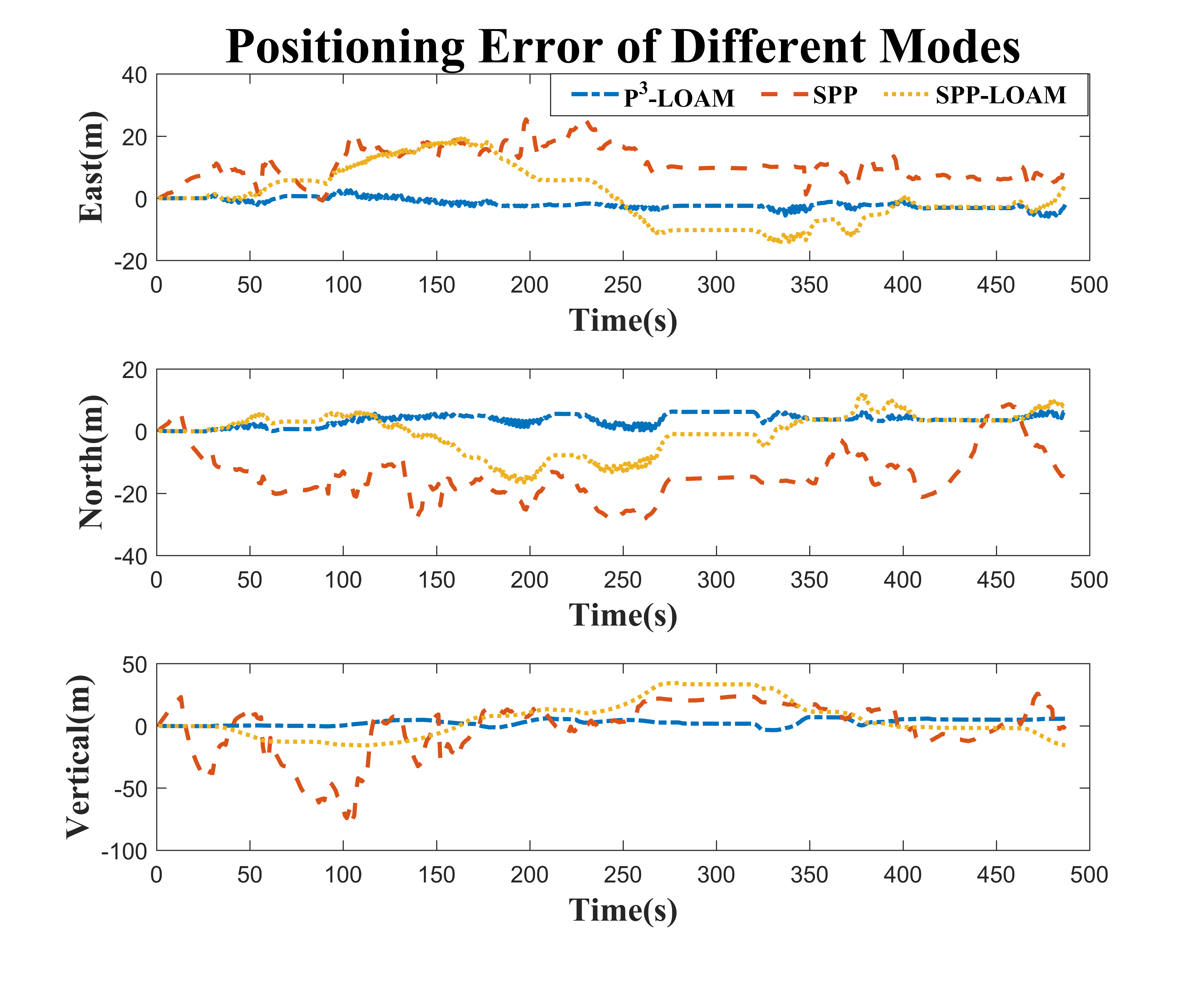
Figure 12: Positioning Error of Different Modes

At last, we count the runtime of the proposed method. The computation loads of the five modules in Fig. 1 are listed in Table IV. It is noted that the CPU of test computer is i7-7700. The LiDAR-SLAM module is derived from ‘LeGO-LOAM’, and other modules bring the additional time consumption about 12% of LiDAR-SLAM. It means that LiDAR-SLAM module is still the dominant computational load of proposed method which is nearly as much as LeGO-LOAM’s computation.

TABLE IV: Runtime of Modules

Modules	Runtime Per Second(ms)
LiDAR-SLAM	340.7
LiDAR-SLAM Covariance Estimation	2.5
PPP Algorithm	17.3
LiDAR-SLAM Assisted GNSS RAIM	10.5
15DoF Variable Optimization	10.2

V Conclusion

In order to obtain robust and reliable positioning results in urban canyon environment, we couple LiDAR and PPP in this paper. For better fusion, we have done the following work: Firstly, we derive an SVD Jacobian based error propagation model to estimate the covariance of LiDAR-SLAM, and the result is evaluated using GNSS covariance and ground truth of trajectory. Secondly, we propose a LiDAR-SLAM assisted GNSS RAIM algorithm, achieving reliable GNSS positioning results in urban canyon environment. Thirdly, P³-LOAM is proposed, combining PPP and LiDAR-SLAM with accurate covariance estimation. The performance of the proposed methods is assessed with a series of experiments: 1) LiDAR-SLAM positioning covariance is evaluated and it is proved to be consistent with that of GNSS. 2) SF-PPP error is gratifyingly controlled using LiDAR-SLAM assisted GNSS RAIM algorithm. 3) We fuse PPP and LiDAR-SLAM to be P³-LOAM, producing better positioning results than any other methods.

However, the availability of PPP in this paper is not satisfactory. In future research, we will work on a tighter coupled LiDAR-SLAM/PPP navigation system so as to improve the availability of PPP in urban canyon environment. In addition, dual-antenna GNSS, or even more antennas, will be set in the vehicle to obtain a global posture for better fusion with LiDAR-SLAM.

Tao Li received the B.S. degree in navigation engineering from Wuhan University, Wuhan, China, in 2018. He is currently pursuing the Ph.D. degree with Shanghai Jiao Tong University, Shanghai, China. His current research interests include Visual-SLAM, LiDAR-SLAM, global navigation satellite systems(GNSS), inertial navigation systems (INS), and information fusion.

Ling Pei received the Ph.D. degree from Southeast University, Nanjing, China, in 2007.From 2007 to 2013, he was a Specialist Research Scientist with the Finnish Geospatial Research Institute. He is currently an Associate Professor with the School of Electronic Information and Electrical Engineering, Shanghai Jiao Tong University. He has authored or co-authored over 90 scientific papers. He is also an inventor of 24 patents and pending patents. His main research is in the areas of indoor/outdoor seamless positioning, ubiquitous computing, wireless positioning, Bio-inspired navigation, context-aware applications, location-based services, and navigation of unmanned systems. Dr. Pei was a recipient of the Shanghai Pujiang Talent in 2014.

Yan Xiang is an assistant professor at Shanghai Jiao Tong University. She obtained her Ph.D. in the Department of Geomatics Engineering at University of Calgary. Her current research interests include inter-frequency and inter-system code and phase bias determination, carrier-phase based ionospheric modeling, and ionospheric augmentation for high precision positioning.

Qi Wu received the B.S. degree in Chongqing University of Posts and Telecommunications, Chongqing, China, in 2018.He received the M.S. degree in Beijing University of Posts and Telecommunications, Beijing, China. He is currently working toward the Ph.D degree in Shanghai Jiao Tong University. His main research interests include visual-SLAM ,LiDAR-SLAM, Multi-sensor fusion.

Songpengcheng Xia received the B.S. degree in navigation engineering from Wuhan University, Wuhan, China, in 2019. He is currently pursuing the Ph.D. degree with Shanghai Jiao Tong University, Shanghai, China. His current research interests include machine learning, inertial navigation, multi-sensor fusion and mixed-reality simulation technology.

Lihao Tao received the B.S. degree in electronic engineering from Beihang University, Beijing, China, in 2018. He is currently pursuing the M.S. degree with Shanghai Jiao Tong University, Shanghai, China. His current research interests include multiple sensors extrinsic calibration(IMU, Camera and LiDAR) and LiDAR-SLAM.

Wenxian Yu received the B.S., M.S., and Ph.D. degrees from the National University of Defense Technology, Changsha, China, in 1985, 1988, and 1993, respectively. From 1996 to 2008, he was a Professor with the College of Electronic Science and Engineering, National University of Defense Technology, where he was also the Deputy Head of the College and an Assistant Director of the National Key Laboratory of Automatic Target Recognition. From 2009 to 2011, he was the Executive Dean of the School of Electronic, Information, and Electrical Engineering, Shanghai Jiao Tong University, Shanghai, China. He is currently a Yangtze River Scholar Distinguished Professor and the Head of the research part in the School of Electronic, Information, and Electrical Engineering, Shanghai Jiao Tong University. His research interests include remote sensing information processing, automatic target recognition, multi-sensor data fusion, etc.

References

- [1] M. Montemerlo, S. Thrun, D. Koller, B. Wegbreit, et al., “Fastslam: A factored solution to the simultaneous localization and mapping problem,” Aaai/iaai, vol. 593598, 2002.
- [2] S. Kohlbrecher, O. V. Stryk, J. Meyer, and U. Klingauf, “A flexible and scalable slam system with full 3d motion estimation,” in 2011 IEEE International Symposium on Safety, Security, and Rescue Robotics, 2011.
- [3] G. Grisetti, C. Stachniss, and W. Burgard, “Improved techniques for grid mapping with rao-blackwellized particle filters,” IEEE Transactions on Robotics, vol. 23, no. 1, pp. 34–46, 2007.
- [4] “Karto slam ros package.” [Online]. Available:http://wiki.ros.org/slam_karto Accessed October 31, 2020.
- [5] L. Carlone, R. Aragues, J. A. Castellanos, and B. Bona, “A linear approximation for graph-based simultaneous localization and mapping,” in Robotics: Science and Systems VII, University of Southern California, Los Angeles, CA, USA, June 27-30, 2011, 2011.
- [6] Z. Ji and S. Singh, “Loam: Lidar odometry and mapping in real-time,” in Robotics: Science and Systems Conference, 2014.
- [7] T. Shan and B. Englot, “Lego-loam: Lightweight and ground-optimized lidar odometry and mapping on variable terrain,” in IEEE/RSJ International Conference on Intelligent Robots and Systems (IROS), pp. 4758–4765, IEEE, 2018.
- [8] J. Behley and C. Stachniss, “Efficient surfel-based slam using 3d laser range data in urban environments,” in Robotics: Science and Systems 2018, 2018.
- [9] X. Chen, A. Milioto, E. Palazzolo, P. Giguere, and C. Stachniss, “Suma++: Efficient lidar-based semantic slam,” in 2019 IEEE/RSJ International Conference on Intelligent Robots and Systems (IROS), 2019.
- [10] P. BESL and N. MCKAY, “A method for registration of 3-d shapes,” IEEE transactions on pattern analysis and machine intelligence, vol. 14, no. 2, pp. 239–256, 1992.
- [11] A. Censi, “An icp variant using a point-to-line metric,” in 2008 IEEE International Conference on Robotics and Automation, pp. 19–25, Ieee, 2008.
- [12] K.-L. Low, “Linear least-squares optimization for point-to-plane icp surface registration,” Chapel Hill, University of North Carolina, vol. 4, no. 10, pp. 1–3, 2004.
- [13] E. B. Olson, “Real-time correlative scan matching,” in 2009 IEEE International Conference on Robotics and Automation, pp. 4387–4393, IEEE, 2009.
- [14] M. Magnusson, The three-dimensional normal-distributions transform: an efficient representation for registration, surface analysis, and loop detection. PhD thesis, Örebro universitet, 2009.
- [15] B. D. Anderson and J. B. Moore, Optimal filtering. Courier Corporation, 2012.
- [16] R. Van Der Merwe, A. Doucet, N. De Freitas, and E. A. Wan, “The unscented particle filter,” in Advances in neural information processing systems, pp. 584–590, 2001.
- [17] F. Gustafsson, F. Gunnarsson, N. Bergman, U. Forssell, J. Jansson, R. Karlsson, and P. J. Nordlund, “Particle filters for positioning, navigation, and tracking,” IEEE Transactions on Signal Processing, vol. 50, no. 2, pp. 425–437, 2002.
- [18] C. Chen, L. Pei, C. Xu, D. Zou, Y. Qi, Y. Zhu, and T. Li, “Trajectory optimization of lidar slam based on local pose graph,” in China Satellite Navigation Conference, pp. 360–370, Springer, 2019.
- [19] R. B. Langley, “Rtk gps,” Gps World, vol. 9, no. 9, pp. 70–76, 1998.
- [20] “Precise point positioning for the efficient and robust analysis of gps data from large networks,” Journal of Geophysical Research, 1997.
- [21] Y. Xiang, Y. Gao, J. Shi, and C. Xu, “Carrier phase-based ionospheric observables using ppp models,” Geodesy and Geodynamics, vol. 8, no. 1, pp. 17–23, 2017.
- [22] H. Hopfield, “Two-quartic tropospheric refractivity profile for correcting satellite data,” Journal of Geophysical research, vol. 74, no. 18, pp. 4487–4499, 1969.
- [23] J. Saastamoinen, “Contributions to the theory of atmospheric refraction,” Bulletin Géodésique (1946-1975), vol. 107, no. 1, pp. 13–34, 1973.
- [24] J. A. Klobuchar, “Ionospheric time-delay algorithm for single-frequency gps users,” IEEE Transactions on aerospace and electronic systems, no. 3, pp. 325–331, 1987.
- [25] “Igs real-time service.” [Online]. Available:http://www.igs.org/rts/products Accessed Semptember 4, 2020.
- [26] Y. Li, Y. Zhuang, X. Hu, Z. Gao, J. Hu, L. Chen, Z. He, L. Pei, K. Chen, M. Wang, X. Niu, R. Chen, J. Thompson, F. Ghannouchi, and N. El-Sheimy, “Toward location-enabled iot (le-iot): Iot positioning techniques, error sources, and error mitigation,” IEEE Internet of Things Journal, pp. 1–1, 2020.
- [27] R. Kalafus, “Receiver autonomous integrity monitoring of gps,” Project Memorandum DOTTSC-FAA-FA-736-1, US DOT Transportation System Center, Cambridge, MA, 1987.
- [28] Z. Gong, R. Ying, F. Wen, J. Qian, and P. Liu, “Tightly coupled integration of gnss and vision slam using 10-dof optimization on manifold,” IEEE Sensors Journal, vol. 19, no. 24, pp. 12105–12117, 2019.
- [29] F. Zhu, Z. Hu, W. Liu, and X. Zhang, “Dual-antenna gnss integrated with mems for reliable and continuous attitude determination in challenged environments,” IEEE Sensors Journal, vol. 19, no. 9, pp. 3449–3461, 2019.
- [30] S. Hewitson and J. Wang, “Extended receiver autonomous integrity monitoring (e raim) for gnss/ins integration,” Journal of Surveying Engineering, vol. 136, no. 1, pp. 13–22, 2010.
- [31] Hyyppa, Juha, Wang, Yiwu, Tang, Jian, Zhu, Lingli, Kukko, and A. and, “Feasibility study of using mobile laser scanning point cloud data for gnss line of sight analysis,” Mobile Information Systems, 2017.
- [32] A. Shetty and G. X. Gao, “Adaptive covariance estimation of lidar-based positioning errors for uavs,” Navigation, vol. 66, no. 2, 2019.
- [33] A. C. B. Chiella, H. N. Machado, B. O. S. Teixeira, and G. A. S. Pereira, “Gnss/lidar-based navigation of an aerial robot in sparse forests,” Sensors, vol. 19, no. 19, p. 4061, 2019.
- [34] L. Chang, X. Niu, T. Liu, J. Tang, and C. Qian, “Gnss/ins/lidar-slam integrated navigation system based on graph optimization,” Remote Sensing, vol. 11, no. 9, 2019.
- [35] A. Geiger, P. Lenz, and R. Urtasun, “Are we ready for autonomous driving? the kitti vision benchmark suite,” in 2012 IEEE Conference on Computer Vision and Pattern Recognition, pp. 3354–3361, IEEE, 2012.
- [36] C. Qian, H. Zhang, W. Li, B. Shu, J. Tang, B. Li, Z. Chen, and H. Liu, “A lidar aiding ambiguity resolution method using fuzzy one-to-many feature matching,” Journal of Geodesy, vol. 94, no. 10, pp. 1–18, 2020.
- [37] G. Wan, X. Yang, R. Cai, H. Li, Y. Zhou, H. Wang, and S. Song, “Robust and precise vehicle localization based on multi-sensor fusion in diverse city scenes,” in 2018 IEEE International Conference on Robotics and Automation (ICRA), pp. 4670–4677, IEEE, 2018.
- [38] M. Joerger and B. Pervan, “Autonomous ground vehicle navigation using integrated gps and laser-scanner measurements,” Proc. ION/IEEE PLANS, 2006.
- [39] G. He, X. Yuan, Y. Zhuang, and H. Hu, “An integrated gnss/lidar-slam pose estimation framework for large-scale map building in partially gnss-denied environments,” IEEE Transactions on Instrumentation and Measurement, 2020.
- [40] A. V. Kanhere and G. X. Gao, “Integrity for gps-lidar fusion utilizing a raim framework,” in Proceedings of ION GNSS Conference, pp. 3145–3155, 2018.
- [41] W. Wen, X. Bai, L.-T. Hsu, and T. Pfeifer, “Gnss/lidar integration aided by self-adaptive gaussian mixture models in urban scenarios: An approach robust to non-gaussian noise,” in 2020 IEEE/ION Position, Location and Navigation Symposium (PLANS), 2020.
- [42] A. U. Shamsudin, K. Ohno, R. Hamada, S. Kojima, T. Westfechtel, T. Suzuki, Y. Okada, S. Tadokoro, J. Fujita, and H. Amano, “Consistent map building in petrochemical complexes for firefighter robots using slam based on gps and lidar,” Robomech Journal, vol. 5, no. 1, p. 7, 2018.
- [43] T. Papadopoulo and M. I. Lourakis, “Estimating the jacobian of the singular value decomposition: Theory and applications,” in European Conference on Computer Vision, pp. 554–570, Springer, 2000.
- [44] K. Chen and Y. Gao, “Real-time precise point positioning using single frequency data,” in ION GNSS, pp. 1514–1523, Citeseer, 2005.
- [45] “Code ionosphere products.” [Online]. Available:http://ftp.aiub.unibe.ch/CODE/ Accessed Semptember 4, 2020.