Connecting 3-manifold triangulations with monotonic sequences of bistellar flips

Abstract

A key result in computational 3-manifold topology is that any two triangulations of the same 3-manifold are connected by a finite sequence of bistellar flips, also known as Pachner moves. One limitation of this result is that little is known about the structure of this sequence—knowing more about the structure could help both proofs and algorithms. Motivated by this, we show that there must be a sequence that satisfies a rigid property that we call “semi-monotonicity”. We also study this result empirically: we implement an algorithm to find such semi-monotonic sequences, and compare their characteristics to less structured sequences, in order to better understand the practical and theoretical utility of this result.

Keywords

Computational topology, 3-manifolds, triangulations, special spines, bistellar flips, Pachner moves

1 Introduction

The homeomorphism problem—given two triangulated 3-manifolds, determine whether they are homeomorphic—is one of the oldest and most important problems in computational low-dimensional topology. Although we now know that there is an algorithm for this problem [10, 17], the algorithm is far too complicated to be implemented, and the best known upper bound on the running time is a tower of exponentials [10]. Nevertheless, we have a variety of techniques that, in practice, often allow us to solve this problem with real data.

• If the given 3-manifolds are not homeomorphic, then we can often distinguish them using efficiently computable invariants such as homology groups, or the Turaev-Viro invariants.

• If the given 3-manifolds are homeomorphic, then we have a range of tools (some of which we mention shortly) that we can use to morph one triangulation into the other without changing the topology.

One important application of these techniques is in building censuses of 3-manifolds: when we generate all possible triangulations up to a certain number of tetrahedra, we end up with many duplicates, so we need to be able to identify (and hence eliminate) such duplicates.

Thus, we have a strong motivation to optimise these techniques. In this paper, we focus on the “yes case”—the task of verifying that two triangulations of the same 3-manifold are indeed homeomorphic. For well-structured manifolds, such as Seifert fibred manifolds or cusped hyperbolic manifolds, we can often do this efficiently using specialised recognition algorithms [13, 19]. However, outside of such special cases, our best known method is to perform an expensive exhaustive search for a sequence of Pachner moves (also often called bistellar flips) that connect the two triangulations.

The Pachner moves are four local moves that can be used to modify a triangulation without changing the underlying topological space; Pachner showed that any two triangulations of the same 3-manifold are connected by a finite sequence of such moves [14]. We focus on two of the four Pachner moves: the 2-3 move, which replaces two distinct tetrahedra attached along a triangular face with three distinct tetrahedra attached around an edge; and the 3-2 move, which is the inverse of the 2-3 move. These moves are illustrated in Figure 1.

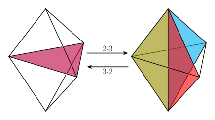
Figure 1: The 2-3 and 3-2 moves. The shaded triangles are the internal faces.

We restrict our attention to these two Pachner moves because every 3-manifold triangulation can be converted into a one-vertex triangulation of the same 3-manifold [9], and because—by independent work of Matveev [12] and Piergallini [15]—any two one-vertex triangulations of the same 3-manifold are connected by a finite sequence of 2-3 and 3-2 moves. (In fact, as we discuss in section 2, the Matveev-Piergallini result extends to more general settings than just one-vertex triangulations of compact 3-manifolds [2, 3, 1].) So, to verify that two triangulations of the same 3-manifold are homeomorphic, it is enough to convert them into one-vertex triangulations, and then search for a sequence of 2-3 and 3-2 moves that connect the two one-vertex triangulations.

The trouble with looking for sequences of 2-3 and 3-2 moves is that such a sequence need not have any particular structure, so we have to resort to a blind search. Thus, one potential way to improve this technique would be to prove the existence of a more structured sequence. For example, we could consider the following types of sequences:

• A monotonic sequence is a sequence consisting precisely of: a series of 2-3 moves, followed by a series of 3-2 moves.

• A semi-monotonic sequence is a sequence consisting precisely of: a series of 2-3 moves, then a series of 2-0 moves (defined in section 2), and then a series of 3-2 moves.

We have a strong theoretical reason to be interested in sequences with extra structure: If, as part of a proof, we would like to assume the existence of a sequence of moves connecting two triangulations, it could be helpful to strengthen this assumption by exploiting the structure of a sequence that is (for instance) monotonic or semi-monotonic.

With this in mind, we show in section 3 (as a special case of a more general theorem) that any two one-vertex triangulations $\mathcal{T}$ and $\mathcal{U}$ of the same 3-manifold are connected by a semi-monotonic sequence. We also briefly discuss how our proof technique could potentially extend to a proof that $\mathcal{T}$ and $\mathcal{U}$ are connected by a monotonic sequence; whether such a monotonic sequence must always exist remains an open problem.

We also study the characteristics of this problem experimentally in section 4. We have implemented algorithms to search for unstructured, monotonic and semi-monotonic sequences that connect triangulations of the same manifold, and we run these over 2984 distinct 3-manifolds with close to 200 million intermediate triangulations. The results suggest that, despite its poorer theoretical bounds, an unstructured blind search gives better practical performance due to requiring fewer additional tetrahedra in intermediate triangulations.

We finish this introduction by noting that monotonic simplification is an old idea originating in knot theory, and ties into the search for (so far elusive) polynomial-time algorithms for unknot and 3-sphere recognition. Broadly, the hope is to find some way to measure the “complexity” of a knot diagram, such that for every diagram $D$ of the unknot, there is a sequence $\varSigma$ of “elementary moves” that “monotonically simplifies” $D$ into a zero-crossing diagram; in this context, the monotonicity requirement means that $\varSigma$ must never increase the complexity of the diagram. Just one major result of this type is known, due to Dynnikov [8]. Roughly speaking, Dynnikov defines a restricted class of knot diagrams called “rectangular diagrams”, and shows that for any rectangular diagram $D$ of the unknot, it is possible to monotonically simplify $D$ to a plain unknotted rectangle.

At first glance, one might hope to get an analogous result involving Pachner moves, with the complexity of a triangulation measured by (for instance) the number of tetrahedra. That is, we might hope that every one-vertex triangulation $\mathcal{T}$ of some 3-manifold $\mathcal{M}$ admits a sequence of 3-2 moves that transforms $\mathcal{T}$ into a triangulation of $\mathcal{M}$ with the smallest possible complexity. However, this naïve idea does not work because many triangulations are “local minima”: they do not have minimum complexity, but at the same time no 3-2 moves are possible. In other words, 2-3 moves are sometimes necessary to simplify a triangulation to its global minimum complexity.

Therefore a “monotonic descent” using only 3-2 moves is not always possible, which motivates our weaker notation of monotonicity here: all the moves that increase complexity occur at the beginning of the sequence, so that once we decrease complexity for the first time, we never increase the complexity again.

2 Preliminaries

2.1 Triangulations and special spines

Triangulations and special spines give two dual ways to represent a 3-manifold. Here, we define these dual notions, and describe how to convert between them. Much of our discussion is based on that in [12] and [16], though we omit the details of some proofs.

A (generalised) triangulation $\mathcal{T}$ is a collection of $n$ tetrahedra, such that each of the $4n$ triangular faces is affinely identified with one of the other triangular faces; intuitively, the $n$ tetrahedra have been “glued together” along their faces to form a 3-dimensional complex. Each pair of identified faces is referred to as a single face of the triangulation. Since the face identifications cause many tetrahedron edges to be identified and many tetrahedron vertices to be identified, we also define an edge of the triangulation to be an equivalence class of identified tetrahedron edges, and a vertex of the triangulation to be an equivalence class of identified tetrahedron vertices. Here we allow multiple edges of the same tetrahedron to be identified, and we allow multiple vertices of the same tetrahedron to be identified.

We call $\mathcal{T}$ a 3-manifold triangulation if its underlying topological space is a 3-manifold. Note that a generalised triangulation $\mathcal{T}$ need not be a 3-manifold triangulation, because it may contain “singularities” at midpoints of edges and at vertices. Depending on the face identifications that make up $\mathcal{T}$, there are two possibilities for an edge $e$.

• If $e$ is identified with itself in reverse, then every small neighbourhood of the midpoint of $e$ will be bounded by a projective plane. In this case, the midpoint of $e$ is a singularity, and $\mathcal{T}$ is not a 3-manifold triangulation.

• Otherwise, every interior point of $e$ will have a small neighbourhood bounded by a sphere, in which case the edge does not produce a singularity.

From now on, we will tacitly assume that no edge is identified with itself in reverse, so that singularities only occur at the vertices of a triangulation.

To see what can happen at a vertex $v$, imagine introducing a small triangle near each tetrahedron vertex that is incident with $v$. As illustrated in Figure 2, we can glue all these triangles together to form a closed surface called the link of $v$. If the link is a sphere, then $v$ is not a singularity, and we call $v$ a material vertex; otherwise, we call $v$ an ideal vertex. A triangulation that satisfies the edge condition above is a 3-manifold triangulation if and only if every vertex is material.

Figure 2: A fragment of the link of $v$, built from triangles.

The motivation for working with these generalised 3-manifold triangulations is that they tend to be smaller, and hence better suited to computation than simplicial complexes. In particular, every 3-manifold admits a one-vertex triangulation: an $n$-tetrahedron triangulation in which all $4n$ tetrahedron vertices are identified to become a single vertex.

Generalised triangulations also give us the flexibility to work with ideal triangulations: triangulations that have one or more ideal vertices. Since each ideal vertex is a singularity, an ideal triangulation represents a pseudo-manifold, rather than a manifold. Having said this, we can also use an ideal triangulation to represent either: the non-compact 3-manifold obtained by deleting the ideal vertices, or the bounded 3-manifold (i.e., 3-manifold with boundary) obtained by truncating the ideal vertices. This idea originated with Thurston’s famous two-tetrahedron ideal triangulation of the figure-eight knot complement [18]. Like one-vertex triangulations, ideal triangulations are particularly suited to computation because they typically require fewer tetrahedra than their non-ideal counterparts.

As mentioned earlier, we can also represent 3-manifolds using the dual notion of a special spine, which is essentially a 2-dimensional complex that captures all the topological information in a 3-dimensional manifold. Let $\mathcal{N}$ be a bounded 3-manifold. A polyhedron (i.e., a 2-dimensional complex) $P$ embedded in the interior of $\mathcal{N}$ is a (possibly non-special) spine of $\mathcal{N}$ if $\mathcal{N}$ is homeomorphic to a regular neighbourhood of $P$ in $\mathcal{N}$.

This definition can be extended to a broader class of manifolds. Let $\mathcal{M}$ be either a closed 3-manifold or a 3-dimensional pseudo-manifold. In essence, we define a spine $P$ of $\mathcal{M}$ by puncturing $\mathcal{M}$ one or more times to get a bounded 3-manifold $\mathcal{M}^{c}$, and taking $P$ to be a spine of $\mathcal{M}^{c}$. More precisely, let $P$ be a polyhedron embedded in $\mathcal{M}$:

• If $\mathcal{M}$ is a closed 3-manifold, then $P$ is a spine of $\mathcal{M}$ if $P$ is a spine of some bounded 3-manifold $\mathcal{M}^{c}$ obtained by deleting one or more disjoint open 3-balls from $\mathcal{M}$.

• If $\mathcal{M}$ is a pseudo-manifold, then $P$ is a spine of $\mathcal{M}$ if $P$ is a spine of some bounded 3-manifold $\mathcal{M}^{c}$ obtained by deleting: a small open neighbourhood of every singularity in $\mathcal{M}$, and possibly one or more disjoint open 3-balls from $\mathcal{M}$.

In either case, we can recover $\mathcal{M}$ from a spine $P$ as follows: first “thicken” $P$ to recover a bounded 3-manifold $\mathcal{M}^{c}$, and then “fill in the holes” in $\mathcal{M}^{c}$ by attaching cones on all the boundary components.

Before defining what it means for a spine of $\mathcal{M}$ to be special, it helps to first see how to convert a triangulation $\mathcal{T}$ of $\mathcal{M}$ into its dual special spine. Start by replacing each tetrahedron in $\mathcal{T}$ with the polyhedron shown in Figure 3; Matveev calls this polyhedron a butterfly. Each butterfly has four edges emanating out from a single central vertex; we can think of the vertex as being dual to a tetrahedron, and the four edges as being dual to the four triangular faces of the tetrahedron. Attached to each pair of edges in the butterfly is a 2-dimensional “wing” that is dual to a tetrahedron edge. Under this notion of duality, the affine face identifications of $\mathcal{T}$ induce a gluing of all these butterflies, yielding a polyhedron $P$ embedded in $\mathcal{M}$; this polyhedron is the special spine dual to $\mathcal{T}$.

To see that $P$ is indeed a spine of $\mathcal{M}$, let $\mathcal{M}^{c}$ be the bounded 3-manifold obtained by deleting the small open neighbourhoods bounded by all the vertex links in $\mathcal{T}$; in other words, $\mathcal{M}^{c}$ is obtained from $\mathcal{T}$ by truncating the vertices of all the tetrahedra in $\mathcal{T}$. Since each truncated tetrahedron is homeomorphic to a regular neighbourhood of its dual butterfly, we can see that $P$ must be a spine of $\mathcal{M}^{c}$, and hence a spine of $\mathcal{M}$.

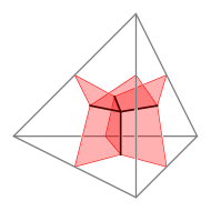
Figure 3: The dual butterfly inside a tetrahedron.

By virtue of being a special spine, it turns out that $P$ determines the corresponding triangulation $\mathcal{T}$ uniquely (see [12] for a proof of this). With this in mind, we finish this section by formally describing what it means for a spine to be special. As an intermediate step, a spine $P$ is simple if every point in $P$ is of one of the following three types:

• A point in $P$ is non-singular if it has a neighbourhood in $P$ homeomorphic to a disc, as illustrated in Figure 4(a) (otherwise, the point is singular).

• A singular point is a triple point if it has a neighbourhood homeomorphic to three half-discs branching out from a common diameter, as illustrated in Figure 4(b).

• A singular point is a vertex if it has a neighbourhood homeomorphic to the butterfly shown in Figure 3. An alternative drawing of the butterfly is shown in Figure 4(c).

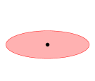
(a) Non-singular point.

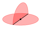
(b) Triple point.

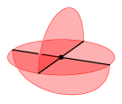
(c) Vertex.

Figure 4: The three types of points allowed in a simple spine.

For a simple spine $P$, observe that: the set of all triple points is a collection of disjoint 1-dimensional components (either open intervals or closed loops), and the set of all non-singular points is a collection of disjoint 2-dimensional components. For $P$ to be a special spine, we require that: the components of triple points are all open intervals (we call each such component an edge), and the components of non-singular points are all open 2-cells (i.e., homeomorphic to an open disc). Given a special spine $P$, the vertices and edges of $P$ together form a 4-regular graph $S_{P}$ called the singular graph of $P$.

2.2 Moves on triangulations and special spines

As mentioned in section 1, the 2-3 and 3-2 moves are local moves that modify a triangulation without changing the underlying manifold or pseudo-manifold. The following series of results tells us (modulo some mild necessary conditions) that two homeomorphic triangulations are always connected by a sequence of such moves.

Theorem 1 (Matveev [12] and Piergallini [15]).

Let $\mathcal{M}$ be a closed $3$-manifold. Let $\mathcal{T}$ and $\mathcal{U}$ be two one-vertex triangulations of $\mathcal{M}$, each with at least two tetrahedra. Then $\mathcal{T}$ is connected to $\mathcal{U}$ by a finite sequence of 2-3 and 3-2 moves.

Theorem 2 (Benedetti and Petronio [2, 3]).

Let $\mathcal{M}$ be a closed $3$-manifold. Let $\mathcal{T}$ and $\mathcal{U}$ be two triangulations $\mathcal{M}$, each with at least two tetrahedra. If $\mathcal{T}$ and $\mathcal{U}$ have the same number of (material) vertices, then $\mathcal{T}$ is connected to $\mathcal{U}$ by a finite sequence of 2-3 and 3-2 moves.

Theorem 3 (Amendola [1]).

Let $\mathcal{M}$ be a closed $3$-manifold or a $3$-dimensional pseudo-manifold. Let $\mathcal{T}$ and $\mathcal{U}$ be two triangulations of $\mathcal{M}$, each with at least two tetrahedra. If $\mathcal{T}$ and $\mathcal{U}$ have the same number (possibly zero) of material vertices, then $\mathcal{T}$ is connected to $\mathcal{U}$ by a finite sequence of 2-3 and 3-2 moves.

Theorems 1, 2 and 3 were originally proved in the dual setting of special spines; a proof of Theorem 3 can also be found in [16]. One advantage of working with special spines is that it is often easier to visualise long sequences of moves in this setting.

In terms of special spines, a 2-3 move involves two distinct vertices connected by an edge $e$. Figure 5 illustrates one way to visualise the 2-3 move: imagine taking a sheet attached to one vertex of $e$, and dragging this sheet along $e$ until it crosses the other vertex. There are many other ways to draw this move, but they are all equivalent under isotopy. We usually simplify our drawings of 2-3 moves, as illustrated in Figure 6.

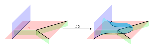
Figure 5: One way to draw the 2-3 move along the red edge $e$.

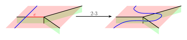
Figure 6: A simplified drawing of the 2-3 move, with the sheet extending upwards from the blue line omitted.

Notice that a 2-3 move creates a new triangle in a spine. Thus, the inverse 3-2 move involves the three distinct vertices of this new triangle. We can visualise this 3-2 move by going backwards in Figures 5 and 6.

In this paper, we also work with a move called the 0-2 move; this move can be found under various names in other sources [1, 11, 12, 15, 16]. In a special spine, a 0-2 move is characterised by a curve $\alpha$ embedded in the closure of a 2-cell $C$, such that the endpoints of $\alpha$ are distinct, and each endpoint lies on an edge of $C$. We can visualise the 0-2 move as a sheet attached to one endpoint being dragged along $\alpha$ until it crosses the other endpoint, as illustrated in Figure 7; this divides $C$ into two new 2-cells $C^{\prime}$ and $C^{\prime\prime}$. Just like with 2-3 moves, there are many equivalent ways to draw the 0-2 move. We usually simplify our drawings of 0-2 moves, as illustrated in Figure 8. By duality, the 0-2 move can also be defined for triangulations, which is where the name comes from (it creates two new tetrahedra), though this is not important for our purposes; see [16] for details.

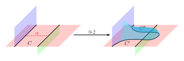
Figure 7: One way to draw the 0-2 move along the red dashed curve $\alpha$.

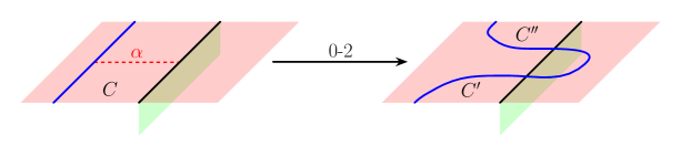
Figure 8: A simplified drawing of the 0-2 move, with the sheet extending upwards from the blue line omitted.

Since the 0-2 move creates a new bigon in a spine, its inverse move—called the 2-0 move—involves the two distinct vertices of this new bigon. We can visualise the 2-0 move by going backwards in Figures 7 and 8. Since the 2-0 move merges the 2-cells $C^{\prime}$ and $C^{\prime\prime}$, we require $C^{\prime}$ and $C^{\prime\prime}$ to be different 2-cells (otherwise, the new 2-component $C$ would be an annulus or Möbius strip, in which case the resulting spine would not be special).

3 Semi-monotonic and monotonic sequences

We recall the following definitions from section 1:

• A semi-monotonic sequence consists precisely of: a series of zero or more 2-3 moves, then a series of zero or more 2-0 moves, and then a series of zero or more 3-2 moves.

• A monotonic sequence consists precisely of: a series of zero or more 2-3 moves, followed by a series of zero or more 3-2 moves.

Our goal in this section is to prove Theorem 4, and then to briefly discuss some possible strategies for proving Conjecture 5.

Theorem 4.

Let $\mathcal{M}$ be a closed $3$-manifold or a $3$-dimensional pseudo-manifold. Let $\mathcal{T}$ and $\mathcal{U}$ be two triangulations of $\mathcal{M}$, each with at least two tetrahedra. If $\mathcal{T}$ and $\mathcal{U}$ have the same number (possibly zero) of material vertices, then $\mathcal{T}$ is connected to $\mathcal{U}$ by a semi-monotonic sequence.

Conjecture 5.

Let $\mathcal{M}$ be a closed $3$-manifold or a $3$-dimensional pseudo-manifold. Let $\mathcal{T}$ and $\mathcal{U}$ be two triangulations of $\mathcal{M}$, each with at least two tetrahedra. If $\mathcal{T}$ and $\mathcal{U}$ have the same number (possibly zero) of material vertices, then $\mathcal{T}$ is connected to $\mathcal{U}$ by a monotonic sequence.

3.1 Matveev’s arch

Our proof of Theorem 4, which we present in section 3.2, uses a variation of a technique from Matveev’s proof of Theorem 1. The construction at the heart of this technique is Matveev’s arch-with-membrane, or arch for short. We have two goals in this section.

• First, we introduce some terminology that will help us describe and work with arches.

• Second, we use this terminology to paraphrase some key ideas from Matveev’s proof, since we will be recycling these ideas in section 3.2.

As illustrated in Figure 9, we can create an arch by performing a 0-2 move along a curve $\alpha$ that connects two points of a single edge. We usually simplify our drawings of arches, as illustrated in Figure 10. By creating an arch, we introduce two new 2-cells: a new monogon, which we call the artificial monogon; and a new bigon (shaded grey in Figures 9 and 10), which we call the artificial 2-cell. An edge is called artificial if it is incident with either the artificial 2-cell or the artificial monogon; otherwise, the edge is called natural.

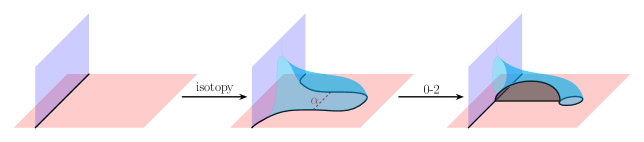
Figure 9: We can create an arch by performing a 0-2 move along the curve $\alpha$. Going backwards, we can destroy an arch by performing a 2-0 move.

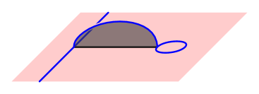
Figure 10: A simplified drawing of an arch, with the sheet attached to the blue edges omitted.

So far, the artificial 2-cell is just a bigon; in this case, the arch has length $0$. Using a series of $\ell$ 0-2 moves followed by $\ell$ 3-2 moves, we can “extend” an arch of length $0$ so that the artificial 2-cell becomes an $(\ell+2)$-gon, in which case the arch has length $\ell$. Figure 11 illustrates how we extend an arch for the case $\ell=4$ (as before, the artificial 2-cell is shaded grey). For general $\ell>0$, the extension procedure involves the following two steps.

• First, we use a series of $\ell$ 0-2 moves to essentially drag the edge of the artificial monogon across $\ell$ (not necessarily distinct) natural edges; in Figure 11, these $\ell$ natural edges are coloured green. These 0-2 moves must occur along a curve embedded in the spine (i.e., the curve never intersects itself); in Figure 11, this curve is drawn as a red dashed line.

• Second, we use a series of $\ell$ 3-2 moves to turn the result of the first step into an arch. In particular, we get a new artificial monogon, and the artificial 2-cell becomes an $(\ell+2)$-gon.

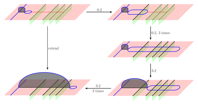
Figure 11: Using a sequence of $\ell$ 0-2 moves followed by $\ell$ 3-2 moves, we can extend an arch of length $0$ to an arch of length $\ell$. Going backwards, we can reduce the length from $\ell$ to $0$ using a sequence of $\ell$ 2-3 moves followed by $\ell$ 2-0 moves.

Observation 6.

An arch of length $\ell$ can be removed using a series of $\ell$ 2-3 moves, followed by $(\ell+1)$ 2-0 moves. Specifically, we can do this using the following two steps.

• First, by going backwards through the extension procedure, we reduce the length to $0$ using a series of $\ell$ 2-3 moves, followed by $\ell$ 2-0 moves.

• We then use an additional 2-0 move (the inverse of the arch-creation move shown in Figure 9) to destroy the arch.

Creating an arch on a spine $P$ is useful because doing so has “minimal impact” on the structure of $P$. To pin down this intuition, we introduce some more terminology. The vertex incident with both the artificial 2-cell and the artificial monogon is called the artificial vertex. A vertex incident with the artificial 2-cell but not with the artificial monogon is called a subdividing vertex; an arch of length $\ell$ yields $\ell+1$ such vertices. A vertex incident with neither the artificial 2-cell nor the artificial monogon is called a natural vertex.

With this terminology in mind, consider the singular graphs $S_{Q}$ and $S_{P}$, where $Q$ denotes a spine obtained by creating an arch of length $\ell$ on $P$. Let $G$ be the graph obtained by deleting the artificial vertex and artificial edges from $S_{Q}$. Observe that:

• every vertex in $S_{P}$ corresponds to a natural vertex in $G$; and

• every edge in $S_{P}$ corresponds to a “chain” of edges that starts at a natural vertex, possibly passes through one or more subdividing vertices, and ends at a natural vertex.

In other words, $G$ is a subdivision of $S_{Q}$. Intuitively, if we “ignore” the artificial vertex and artificial edges, then the singular graphs $S_{Q}$ and $S_{P}$ can be considered “more-or-less equivalent”. Thus, we can think of the spine $Q$ as being “just like $P$, but with an extra arch”.

We now outline how Matveev uses arches in his proof of Theorem 1 (see [12] for more details), since a similar idea will be useful for us in section 3.2. Here, we rephrase Matveev’s idea in a way that is better suited to our purposes. Prior to proving Theorem 1, Matveev establishes the following (non-trivial) facts.

• A 0-2 move on a special spine can be replaced by a sequence (not necessarily monotonic) of 2-3 and/or 3-2 moves. Going backwards, if a 2-0 move results in a special spine, then it can be replaced by a sequence of 2-3 and/or 3-2 moves.

• If $P$ and $Q$ are special spines of the same $3$-manifold, each with at least two vertices, then $P$ is connected to $Q$ by a sequence $\varSigma$ of 2-3, 3-2, 0-2 and/or 2-0 moves.

From here, Matveev proceeds by turning the sequence $\varSigma$ into a new sequence that only uses 2-3 and 3-2 moves.

Although the 0-2 moves in $\varSigma$ can always be replaced by 2-3 and 3-2 moves, we might not be able to replace all of the 2-0 moves, because a 2-0 move could yield a spine that is not special. Matveev circumvents this issue by creating an arch every time a 2-0 move is supposed to be performed. To see how this works, consider a 2-0 move $\vartheta$ that turns a spine $P$ into another spine $Q$. Instead of performing the move $\vartheta$, we can perform the 2-3 move illustrated in Figure 12, which turns $P$ into a spine that is just like $Q$ except it has an extra arch of length $1$. Note that this 2-3 move is always possible, since we must initially have two distinct vertices to perform the 2-0 move $\vartheta$. (In [12], Matveev actually creates the arch using a 0-2 move followed by a 3-2 move. Our 2-3 move gives the same result, but is more useful for our purposes in section 3.2.)

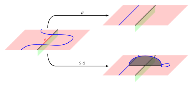
Figure 12: Instead of turning $P$ into $Q$ by performing the 2-0 move $\vartheta$, we can perform a 2-3 move along the red edge $e$ to turn $P$ into a spine that looks like $Q$ with an extra arch.

As we have already mentioned, Matveev’s idea is to replace every 2-0 move by creating an arch in the manner just described. The extra arches that arise in this way can be moved around quite freely using 2-3, 3-2 and 0-2 moves, so that they never prevent us from performing any of the 2-3, 3-2 and 0-2 moves in $\varSigma$; the specific details are unimportant here, but it is worth noting that we rely on a slight variation of this idea in section 3.2. At the end, we can use Observation 6 to remove all the extra arches using 2-3 and 2-0 moves; it is not hard to see that every intermediate spine in this removal process must be special, which means that the 2-0 moves can be realised by 2-3 and 3-2 moves. In this way, Matveev turns $\varSigma$ into a sequence consisting only of 2-3 and 3-2 moves.

3.2 Proof of Theorem 4

We first use Matveev’s arch, together with the related ideas discussed above, to prove the following lemma. We then use this lemma to prove Theorem 4.

Lemma 7.

Let $P$ and $Q$ be two spines, and suppose $P$ is connected to $Q$ by a sequence $\gamma,\delta_{1},\ldots,\delta_{k}$, where $\gamma$ is a 3-2 move and each $\delta_{i}$ is a 2-3 move. Then $P$ is connected to $Q$ by a sequence consisting precisely of: a series of 2-3 moves, followed by a series of 2-0 moves.

• Let $Q_{0}$ denote the spine obtained from $P$ by applying the 3-2 move $\gamma$, and for each $i\in\{1,\ldots,k\}$ let $Q_{i}$ denote the spine obtained from $Q_{i-1}$ by applying the 2-3 move $\delta_{i}$ (so, in particular, $Q_{k}=Q$). Our strategy is to show that there is a sequence of 2-3 moves that transforms $P$ through a series of spines $P_{0},\ldots,P_{k}$, such that each $P_{i}$ looks just like $Q_{i}$ but with an extra arch. We can then use Observation 6 to remove the extra arch in $P_{k}$, and hence transform $P_{k}$ into $Q$.

  We transform $P$ into $P_{k}$ using the following steps.

  1. Starting with $P$, instead of performing the 3-2 move $\gamma$, we perform the two 2-3 moves shown in Figure 13. Note that each of these 2-3 moves involves two distinct vertices:

     • the first 2-3 move involves two of the three vertices involved in the 3-2 move $\gamma$; and

     • the second 2-3 move involves one vertex involved in the 3-2 move $\gamma$, and one vertex that is created by the first 2-3 move.

     This yields a new spine $P_{0}$ that looks just like $Q_{0}$ but with an extra arch (of length $1$).

  2. For each $i\in\{1,\ldots,k\}$, let $u_{i}$ and $v_{i}$ denote the two vertices of $Q_{i-1}$ involved in the 2-3 move $\delta_{i}$, and let $e_{i}$ denote the edge along which we perform $\delta_{i}$. Since $P_{i-1}$ looks like $Q_{i-1}$ with an extra arch, we know that:

     • $u_{i}$ corresponds to a natural vertex $u_{i}^{\prime}$ in $P_{i-1}$;

     • $v_{i}$ corresponds to a natural vertex $v_{i}^{\prime}$ in $P_{i-1}$; and

     • $e_{i}$ corresponds to a chain $e_{i}^{\prime}$ of edges connecting $u_{i}^{\prime}$ and $v_{i}^{\prime}$, with any intermediate vertices in this chain being subdividing vertices.

     Note that the vertices appearing along the chain $e_{i}^{\prime}$ are all distinct, so we can always perform 2-3 moves involving a pair of consecutive vertices in this chain. In particular, if the chain $e_{i}^{\prime}$ consists of just a single edge, then we can perform the move $\delta_{i}$ on $P_{i-1}$ by performing a 2-3 move along this edge; this yields a new spine $P_{i}$ that looks like $Q_{i}$ with an extra arch (note that in this case, the length of the arch remains unchanged).

     Otherwise, if the chain $e_{i}^{\prime}$ consists of multiple edges, then each subdividing vertex in the chain basically corresponds to a “fragment” of the extra arch that obstructs the move $\delta_{i}$. In this case, we shift a fragment out of the way by performing a 2-3 move involving:

     • a natural vertex $w$ at one endpoint of $e_{i}^{\prime}$ (so either $w=u_{i}^{\prime}$ or $w=v_{i}^{\prime}$); and

     • the subdividing vertex that is connected to $w$ in $e_{i}^{\prime}$.

     This idea is illustrated in Figure 14. Shifting in this way yields a new spine that still looks like $Q_{i-1}$ with an extra arch; by an abuse of notation, we still refer to the new spine as $P_{i-1}$, and we still use $e_{i}^{\prime}$ to refer to the chain of edges corresponding to the edge $e_{i}$. Our “shifting move” has two main effects on the spine $P_{i-1}$.

     • First, the length of the extra arch increases by one.

     • Second, the number of subdividing vertices in the chain $e_{i}^{\prime}$ decreases by one.

     So, by shifting fragments away one at a time, we eventually reduce the chain $e_{i}^{\prime}$ to a single edge connecting $u_{i}^{\prime}$ and $v_{i}^{\prime}$. We can therefore perform the move $\delta_{i}$ on $P_{i-1}$ by performing a 2-3 move along the edge in $e_{i}^{\prime}$. This yields a new spine $P_{i}$ that looks like $Q_{i}$ with an extra arch (though this time the length of the arch will have increased).

  In the end, we get a sequence of 2-3 moves that transforms $P$ into a spine $P_{k}$ that looks just like $Q$ but with an extra arch; let $\ell$ denote the length of this arch. By removing this arch using Observation 6, we therefore transform $P_{k}$ into $Q$ using a series of $\ell$ 2-3 moves followed by $(\ell+1)$ 2-0 moves. ∎

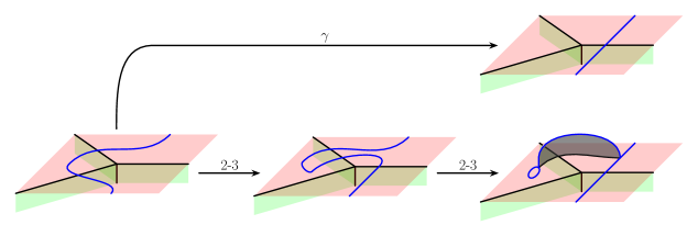
Figure 13: We “copy” the initial 3-2 move $\gamma$ using two 2-3 moves, at the cost of introducing an extra arch.

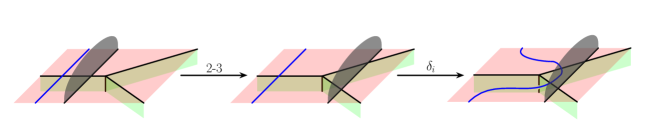
Figure 14: The 2-3 move $\delta_{i}$ is initially obstructed by the grey arch fragment. To circumvent this issue, we first shift the fragment out of the way using a 2-3 move, and then perform $\delta_{i}$.

See 4

• Given any sequence $\varSigma$ of 2-3, 3-2 and 2-0 moves, let $\delta_{\varSigma}$ denote the last 2-3 move in $\varSigma$. We call such a sequence benign if all the 2-0 moves occur consecutively in a (possibly empty) sequence appearing immediately after $\delta_{\varSigma}$; in particular, we consider a sequence consisting only of 2-3 and 3-2 moves to be benign.

  With this in mind, let $P$ be the special spine dual to $\mathcal{T}$, and $Q$ the special spine dual to $\mathcal{U}$. By the dual statement of Amendola’s result (Theorem 3), we know that $P$ is connected to $Q$ by a sequence of 2-3 and 3-2 moves. We will show that this benign sequence can be replaced with a semi-monotonic sequence. To do this, define $n(\varSigma)$, for any benign sequence $\varSigma$ connecting $P$ to $Q$, to be the number of 3-2 moves in $\varSigma$ that occur before $\delta_{\varSigma}$. Observe that $n(\varSigma)=0$ if and only if $\varSigma$ is semi-monotonic. So, to show that $P$ is connected to $Q$ by a semi-monotonic sequence, it suffices to show that given any benign sequence $\varSigma$ with $n(\varSigma)>0$, we can build a new benign sequence $\varSigma^{\prime}$ such that $n(\varSigma^{\prime})=n(\varSigma)-1$.

  To this end, suppose $n(\varSigma)>0$, and let $\gamma$ be the last 3-2 move in $\varSigma$ that occurs before $\delta_{\varSigma}$. Consider the subsequence of moves starting with $\gamma$ and ending with $\delta_{\varSigma}$; this subsequence consists precisely of: a single 3-2 move (namely $\gamma$), followed by a series of 2-3 moves ending with $\delta_{\varSigma}$. By Lemma 7, we can replace this subsequence with a new subsequence consisting precisely of: a series of 2-3 moves, followed by a series of 2-0 moves. This yields a new benign sequence $\varSigma^{\prime}$ with exactly the required property: $n(\varSigma^{\prime})=n(\varSigma)-1$. ∎

3.3 From semi-monotonic to monotonic sequences

In essence, we require 2-0 moves in Theorem 4 in order to create and manage our arches, and we need these arches to avoid intermediate spines that are not special (and therefore not dual to triangulations). However, we conjecture that these 2-0 moves are not actually necessary:

See 5

One possible strategy for proving Conjecture 5 would be to prove the following claim, which would imply that a semi-monotonic sequence can be replaced by a monotonic one.

Conjecture 8.

Let $P$ and $Q$ be two special spines, and suppose $P$ is connected to $Q$ by a sequence of 2-0 moves. Then $P$ is connected to $Q$ by a monotonic sequence.

Alternatively, a more concrete strategy for proving Conjecture 5 could be to use essentially the same proof as for Theorem 4, but replacing Lemma 7 with the following stronger claim.

Conjecture 9.

Let $P$ and $Q$ be two spines, and suppose $P$ is connected to $Q$ by a sequence $\gamma,\delta_{1},\ldots,\delta_{k}$, where $\gamma$ is a 3-2 move and each $\delta_{i}$ is a 2-3 move. Then $P$ is connected to $Q$ by a monotonic sequence.

A proof of Conjecture 9 has so far proven elusive. We could follow a similar proof strategy to that used for Lemma 7, but there is an obvious obstacle: we currently rely on using a combination of 2-3 and 2-0 moves to remove the extra arch at the end (recall Observation 6), so we would instead need to find a way to remove an arch using a monotonic sequence.

4 Experimental results

As discussed in the introduction, when verifying that two triangulations are indeed homeomorphic, in practice we often need to resort to a blind search for a sequence of Pachner moves. Therefore one reason to be interested in monotonic and semi-monotonic sequences is to allow us to perform a more targeted search. In this section, we compare these “blind” and “targeted” approaches by testing how efficiently they find sequences connecting pairs of minimal triangulations of the same 3-manifold. Here, a minimal triangulation of a 3-manifold $\mathcal{M}$ means a triangulation of $\mathcal{M}$ with the smallest possible number of tetrahedra.

Our experimental data set is the census of all minimal triangulations of closed irreducible 3-manifolds with $n\leq 11$ tetrahedra [5]. We use only manifolds with more than one minimal triangulation; in the orientable case we also restrict ourselves to $n\geq 3$ (to avoid special cases) and $n\leq 10$ (to keep the experiments feasible). The resulting data set contains 2 628 orientable and 356 non-orientable manifolds, with 17 027 minimal triangulations in total.

For each manifold, we attempt to connect all of its minimal triangulations with Pachner moves using three algorithms: a blind search, a monotonic search, and a semi-monotonic search. The blind search attempts all possible sequences of 2-3 and 3-2 moves that never exceed $n+h$ tetrahedra, for increasing values of $h$. The monotonic search considers all sequences of $h$ 2-3 moves up from each minimal triangulation, for increasing values of $h$, until these sequences meet at some common triangulation(s). The semi-monotonic search is similar, except that after each individual 2-3 move it then attempts to connect with other increasing 2-3 paths using all possible sequences of 2-0 moves.

Each of these searches can generate enormous numbers of triangulations, leading to high time and memory costs, and so the algorithms must be implemented carefully; here we use isomorphism signatures to avoid revisiting triangulations, and union-find to detect when sequences of moves intersect. See [6] for details. All code was written using Regina [4, 7].

We measure the performance of each algorithm by the total number of triangulations that it constructs, since this directly determines both the running time and memory usage. We removed one manifold from our data set because the monotonic search exceeded $50\,000\,000$ triangulations (a limit imposed to avoid exhausting memory). Our key observations:

• In every case, the monotonic and semi-monotonic search generated the same number of triangulations from 2-3 and 3-2 moves, and required the same additional number of tetrahedra $h$. This means that in practice the 2-0 moves are unnecessary, lending further weight to Conjecture 5.

• For $\sim 88\%$ of manifolds, none of the triangulations generated in the semi-monotonic search supported 2-0 moves at all. For the remaining minority of manifolds, the number of additional triangulations generated from 2-0 moves is consistently small, though the portion does rise slowly; see Figure 15 which plots these numbers on a log scale (each data point represents a single manifold). This suggests that, though the 2-0 moves are unnecessary, they are also not costly.

  

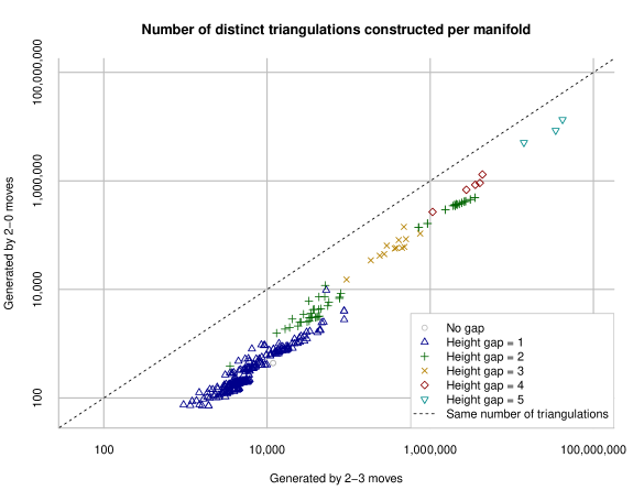
  Figure 15: Measuring the cost of 2-0 moves in the semi-monotonic search.

• The single most important factor in the performance is the height gap: the difference between the number $h$ of additional tetrahedra required in each search type. Figure 16 compares the blind and monotonic searches on a log scale, and categorises the manifolds by this height gap; we see that each additional tetrahedron costs roughly an additional order of magnitude.

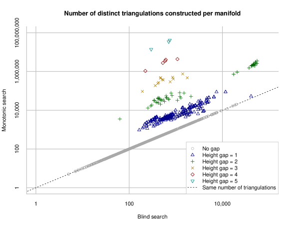
Figure 16: Comparing performance of the blind and monotonic searches.

So, the clear message is: when attempting to connect two triangulations in practice to prove that they are homeomorphic, we should use a blind search, because the cost of searching through a larger set of triangulations with $n+h$ tetrahedra is found to be significantly cheaper than the cost of extending the search to $n+h+1$ tetrahedra.

This also highlights the importance of experimental testing: the blind search could theoretically run through $e^{O(n\log n)}$ triangulations at every new height, whereas the monotonic search only searches through $O(n^{h})$ triangulations at height $h$; although the former cost is more expensive in theory, it is shown to be cheaper in practice.

We see then that the main benefit of monotonicity is theoretical: when working in a proof with two triangulations of the same 3-manifold, instead of just assuming there is an arbitrary path of 2-3 and 3-2 moves with no particular structure, we may strengthen this assumption to use a semi-monotonic path instead.

Having said this, we can make two final observations:

• In most of our test cases, the height gap is small: of our 2984 triangulations, only 81 had a height gap over $2$. Thus the performance gap we see, though significant when it occurs, appears uncommon.

• In all of our test cases, the heights themselves are surprisingly small: $\leq 3$ for every blind search, and $\leq 7$ for every monotonic search except the one that was terminated early.

It is important to note that our experiments may be subject to the tyranny of small numbers: whilst we cover hundreds of millions of intermediate triangulations, these triangulations are all relatively small. Due to the exponential time and memory requirements, obtaining exact data such as ours quickly becomes impossible as the number of tetrahedra grows.

References

- [1] Gennaro Amendola. A calculus for ideal triangulations of three-manifolds with embedded arcs. Math. Nachr., 278(9):975–994, 2005.
- [2] Riccardo Benedetti and Carlo Petronio. A finite graphic calculus for -manifolds. Manuscripta Math., 88(3):291–310, 1995.
- [3] Riccardo Benedetti and Carlo Petronio. Branched standard spines of -manifolds, volume 1653 of Lecture Notes in Mathematics. Springer-Verlag, 1997.
- [4] Benjamin A. Burton. Introducing Regina, the 3-manifold topology software. Experiment. Math., 13(3):267–272, 2004.
- [5] Benjamin A. Burton. Detecting genus in vertex links for the fast enumeration of 3-manifold triangulations. In ISSAC 2011: Proceedings of the 36th International Symposium on Symbolic and Algebraic Computation, pages 59–66. ACM, 2011.
- [6] Benjamin A. Burton. Simplification paths in the Pachner graphs of closed orientable 3-manifold triangulations. arXiv Mathematics e-prints, 2011. arXiv:1110.6080.
- [7] Benjamin A. Burton, Ryan Budney, William Pettersson, et al. Regina: Software for low-dimensional topology. http://regina-normal.github.io/, 1999–2020.
- [8] Ivan A. Dynnikov. Arc presentations of links. monotonic simplification. Fund. Math., 190:29–76, 2006.
- [9] William Jaco and J. Hyam Rubinstein. 0-efficient triangulations of 3-manifolds. J. Differential Geom., 65(1):61–168, 2003.
- [10] Greg Kuperberg. Algorithmic homeomorphism of 3-manifolds as a corollary of geometrization. Pacific J. Math., 301(1):189–241, 2019.
- [11] Sergei V. Matveev. Transformations of special spines and the Zeeman conjecture. Izv. Akad. Nauk SSSR Ser. Mat., 51(5):1104–1116, 1987. [Math. USSR-Izv., 31(2):423–-434, 1988].
- [12] Sergei V. Matveev. Algorithmic Topology and Classification of 3-Manifolds, volume 9 of Algorithms and Computation in Mathematics. Springer-Verlag, second edition, 2007.
- [13] Sergei V. Matveev et al. Manifold recognizer. http://www.matlas.math.csu.ru/?page=recognizer, accessed August 2012.
- [14] Udo Pachner. P.L. homeomorphic manifolds are equivalent by elementary shellings. Europ. J. Combinatorics, 12(2):129–145, 1991.
- [15] Riccardo Piergallini. Standard moves for standard polyhedra and spines. In III Convegno Nazionale Di Topologia: Trieste, 9-12 Giugno 1986 : Atti, number 18 in Rend. Circ. Mat. Palermo (2) Suppl., pages 391–414, 1988.
- [16] J. Hyam Rubinstein, Henry Segerman, and Stephan Tillmann. Traversing three-manifold triangulations and spines. Enseign. Math., 65(1/2):155–206, 2019.
- [17] Peter Scott and Hamish Short. The homeomorphism problem for 3-manifolds. Algebr. Geom. Topol., 14(4):2431–2444, 2014.
- [18] William P. Thurston. The geometry and topology of three-manifolds, 1978. Lecture notes.
- [19] Jeffrey R. Weeks. Convex hulls and isometries of cusped hyperbolic -manifolds. Topology Appl., 52(2):127–149, 1993.