Sharp Bounds in the Latent Index Selection Model

Abstract

A fundamental question underlying the literature on partial identification is: what can we learn about parameters that are relevant for policy but not necessarily point-identified by the exogenous variation we observe? This paper provides an answer in terms of sharp, analytic characterizations and bounds for an important class of policy-relevant treatment effects, consisting of marginal treatment effects and linear functionals thereof, in the latent index selection model as formalized in Vytlacil [2002]. The sharp bounds use the full content of identified marginal distributions, and analytic derivations rely on the theory of stochastic orders. The proposed methods also make it possible to sharply incorporate new auxiliary assumptions on distributions into the latent index selection framework. Empirically, I apply the methods to study the effects of Medicaid on emergency room utilization in the Oregon Health Insurance Experiment, showing that the predictions from extrapolations based on a distribution assumption (rank similarity) differ substantively and consistently from existing extrapolations based on a parametric mean assumption (linearity). This underscores the value of utilizing the model’s full empirical content in combination with auxiliary assumptions.

Keywords: instrumental variables, latent index selection model, marginal treatment effects, partial identification, sharp bounds, counterfactuals, extrapolation, second-order stochastic dominance, stochastic ordering, majorization, Oregon Health Insurance Experiment
JEL Classification: C14, C26, C50

1 Introduction

The method of instrumental variables (IV) forms a cornerstone of modern econometrics. In the basic program evaluation problem with imperfect compliance, Imbens and Angrist [1994] show that IV yields an average causal effect of treatment on outcomes when the instrument shifts treatment monotonically; this is the influential Local Average Treatment Effect (LATE) on the subgroup of compliers, whose treatment decisions depend on the instrument. By definition, the group of compliers — and thus the identified causal effect — are inextricably tied to the instrument at hand.

As a consequence, the variation that identifies a quantity of interest is not always the variation that is observed. For example, typical quasi-experimental settings do not provide a choice of instrument — the instrument may be too coarse, or it may not correspond to a counterfactual of interest. Even when such a choice is available, as in the design of experiments, it is often constrained in practice by other considerations such as statistical power or limited resources. Furthermore, assuming that a treatment effect of interest is equal to the one that is identified precludes selection on unobservables, which belies the purpose of the model. This motivates an alternative structural approach to identification based on a marginal treatment effect (MTE) function in an empirically equivalent latent index selection model [Heckman and Vytlacil [1999, 2005]; Vytlacil [2002]]. A fundamental question, raised recently within this paradigm by Mogstad, Torgovitsky, and Santos [2018], is the following: what can we learn about parameters that are relevant for policy but not necessarily point-identified by the exogenous variation we observe? The question nests a variety of applications, including inference about counterfactuals, inference about internally valid parameters that may not be point-identified, and specification tests.

This paper provides an answer in terms of sharp, analytically-derived bounds for an important class of target parameters in the latent index selection model, as formulated in Vytlacil [2002]. Thus the paper builds most directly on the recent yet already influential contribution of Mogstad et al. [2018], who introduce a computational framework for counterfactual inference that utilizes — and exhausts — the identifying power of observed conditional means for a closely related class of target parameters. A starting point of the present contribution is that consistency with conditional means — henceforth, mean consistency — does not exhaust the identifying power of the fully independent latent index selection model, which is frequently applicable in settings with (quasi)random assignment. In the absence of further assumptions or structure, mean consistency only provides information about point-identified mean outcomes and the LATE among compliers. In addition to means, the empirically equivalent LATE model identifies distributions of potential outcomes among certain subpopulations [Imbens and Rubin [1997], Abadie [2002]]. Consistency with identified distributions — henceforth, distribution consistency — imposes additional restrictions on target parameters, yielding some information about parameters other than the observed means and the LATE, even in the basic model.

As a motivating example, suppose an experiment subsidized treatment relative to a status quo, and a policy-maker is now interested in counterfactual local average treatment effects under intermediate subsidies. In particular, consider a policy that is expected to reduce treatment takeup by, say, 10% among experimental compliers. Information about conditional means does not bound the local average treatment effect under the policy in the latent index selection model without further structure or assumptions. Nevertheless, the model imposes such bounds because it identifies the marginal distributions of potential outcomes among compliers. What matters then for the policy-relevant treatment effect is which 10% of compliers “drop out” of treatment relative to the experiment subsidy. In one extreme, the dropouts are those in the highest decile of the complier treated outcome distribution and in the lowest decile of the untreated outcome distribution; in the other extreme, the reverse is true. This pair of extreme scenarios yield the sharp bounds on the effect of the policy because the model does not impose any bounds on the joint distribution of complier outcomes beyond consistency with the identified marginals.

This basic intuition of “trimming” identified outcome distributions is related to Lee [2009]. In a model of sample selection where a randomized treatment shifts sample selection monotonically, he derives sharp bounds for the average treatment effect among the always-sampled by thus bounding their average treated outcome. One significant difference in the present model with imperfect compliance is that the trimming intuition is “two-sided” because neither average potential outcome need be point-identified among a given subgroup.

The intuition is also generalized to analytically obtain sharp bounds on a class of weighted average treatment effects — technically, linear functionals of the MTE function — via the theory of stochastic orders. More specifically, the sharp set of possible marginal treatment effect functions is characterized in terms of a mean consistency and a second-order stochastic dominance condition relative to the distribution of countermonotonic treatment effects among compliers (Theorem 1). The importance of the countermonotonic effect (among compliers) is that it pairs the highest treated outcomes with the lowest untreated outcomes and vice versa, thus yielding the extremal treatment effect distribution consistent with the identified marginals from which all candidate MTE functions can be generated. Sharp lower and upper bounds on weighted average treatment effects are obtained by rearranging an extremal marginal treatment effect function to be co- or counter-monotonic with the weighting function (Theorem 2). The first result relies on properties of the convex stochastic order, and the second also on properties of the supermodular stochastic order.

These results also relate and contribute to a literature on the identification of the treatment effect distribution and its functionals in the case of perfect compliance [Heckman et al. [1997], Fan and Park [2010], Firpo and Ridder [2019]], because in this case the quantile function of treatment effects constitutes a possible MTE function. I elaborate on this connection in Subsection 3.4 after a presentation of the main results. Furthermore, these results naturally suggest a complete graphical representation in terms of uniformly sharp bounds (Proposition 1), which relates the quality of counterfactual inference to a well-known measure of statistical dispersion (the Gini coefficient) and yields a specification test for further parametric assumptions.

A central feature of the basic latent index selection model is its lack of assumptions on the relationship between selection and potential outcomes. Unsurprisingly, this can translate into weak inference over counterfactual parameters, especially as they become increasingly different from the ones point-identified by the observed data. For example, reconsider the problem of bounding the effects of intermediate subsidies. The data-generating processes that attain the non-parametric bounds exhibit two extreme properties, which may be implausible in many applications. First, potential outcomes among compliers are perfectly countermonotonic: those with the highest realized outcomes if treated would have obtained the lowest outcomes if not treated, and vice versa. Second, compliers (negatively) select perfectly into treatment based on the resulting extremal treatment effects. Additionally, the basic model does not provide information on counterfactual treatment effects beyond compliers because one of the underlying potential outcomes is always unobserved. Economic theory suggests a number of auxiliary assumptions a researcher may consider in order to sharpen the non-parametric bounds. In their recent contribution, Mogstad et al. [2018] incorporate a variety of conditional mean assumptions into their computational framework in order to tighten partial identification.

Another contribution of this paper is that the basic MTE characterizations can be used to incorporate and exhaust the content of additional distribution assumptions, as evidenced by two simple extensions. In the first extension, I aggregate over observed covariates and provide a sharp policy-relevant interpretation of the aggregated bounds. Covariate information improves identification using marginal distributions by restricting the set of feasible joint distributions of potential outcomes. In the second extension, I sharply incorporate the rank similarity assumption of Chernozhukov and Hansen [2005]. Incorporating this assumption into the latent index framework confers several advantages. First, the latent index framework defines a variety of policy-relevant treatment effects, which are typically not point-identified under rank similarity alone, even when the unconditional potential outcome distributions are point-identified. Second, the added structure of the framework permits an alternative identification strategy — intuitively, extrapolation from compliers — that relaxes the need for continuity of outcomes in the existing method. This is important for the subsequent empirical application, in which some outcomes are discrete and all outcomes have a mass point at zero. Third, the added empirical content of the rank similarity assumption is again summarized compactly and graphically in terms of uniformly sharp bounds [as in Proposition 1], even though conditional marginal distributions may no longer be fully identified. Thus the framework provides simple ways to compare or combine further assumptions with rank similarity, as well as providing an alternative test of (unconditional) rank similarity, as in Dong and Shen [2018] and Frandsen and Lefgren [2018].

Empirically, I apply the methods using publicly available data from the Oregon Health Insurance Experiment (OHIE) [Finkelstein [2013]]. The OHIE, which extended Medicaid to a randomly selected group of uninsured, low-income adults in Oregon, is unique in the experimental evidence it provides on the impacts of insurance coverage on health outcomes. Yet many questions of policy interest — for example, the effects of broader expansions, encapsulated in proposals of “Medicare for All” — require extrapolation of point-identified treatment effects to different subpopulations. Specifically, I revisit the question of how insurance coverage affects emergency room (ER) utilization. Previous analyses using the OHIE data find a positive effect of health insurance on ER visits across a range of complier subpopulations [Taubman [2014]], yet predict negative effects across various measures of ER utilization for expansions of Medicaid to the never-treated [Kowalski [2016]]; these predictions are based on the linear extrapolation method of Brinch et al. [2017]. My main empirical contribution is to show that an extrapolation based on the distribution assumption of rank similarity predicts positive (in one case, nonnegative) average treatment effects among the never-treated, which for some outcomes are even larger than the average treatment effect among compliers. Thus distribution information and assumptions may provide substantively different predictions than the ones obtained from mean information and assumptions alone.

The paper proceeds as follows. Section 2 reviews the latent index selection model and the identification problem. Section 3 provides the main results and relates them in more detail to the previous literature. Section 4 extends the results to auxiliary information and assumptions. Section 5 provides an empirical application using the publicly available data from the Oregon Health Insurance Experiment. Section 6 concludes.

2 Framework

2.1 Model

In what follows, random variables are defined on a common probability space $(\Omega,\mathcal{F},P)$ with (cumulative) distribution function $F$. For a given random variable $X$, let $Q_{X}:[0,1]\to\mathds{R}$ denote its quantile function, $Q_{X}(q)=\inf\{x:F_{X}(x)\geq q\}$, and let $I_{X}:[0,1]\to\mathds{R}$ denote its integrated quantile function (IQF), $I_{X}(q)=\int_{0}^{q}\,Q_{X}(s)\,ds$. A random variable $X$ is said to second-order stochastically dominate another random variable $X^{\prime}$, written $X\succeq_{SSD}X^{\prime}$, if $I_{X}(q)\geq I_{X^{\prime}}(q)$ for all $q\in[0,1]$. Two random variables $X$ and $X^{\prime}$ defined on the same probability space are comonotonic if $(X,X^{\prime})\stackrel{{\scriptstyle d}}{{=}}(Q_{X}(V),Q_{X^{\prime}}(V))$ and countermonotonic if $(X,X^{\prime})\stackrel{{\scriptstyle d}}{{=}}(Q_{X}(V),Q_{X^{\prime}}(1-V))$, where $(X,X^{\prime})$ denotes the random vector, $\stackrel{{\scriptstyle d}}{{=}}$ denotes equality in distribution, and $V\sim U[0,1]$. In words, comonotonic random variables can be thought of as nondecreasing functions of a single random variable $V$ and thus exhibit perfect positive dependence; analogously, countermonotonic random variables exhibit perfect negative dependence. The second-order stochastic dominance relation and monotonic random variables will play an important role in subsequent characterizations.

Proceeding with the variables of the model, let $D$ denote the binary realized treatment decision and let $Z$ denote an exogenous correlate of the treatment decision, or instrument. For simplicity of notation and to crystallize the intuition of the partial identification approach, I henceforth assume that the instrument $Z$ is also binary. For example, this occurs in policy evaluation settings with noncompliance, e.g. Section 5. In this case $Z$ is the treatment assignment, and I henceforth adopt this terminology. Let $D_{z}$ denote the potential treatment decision that would be observed if the treatment assignment were exogenously set to $z$. Note that the realized treatment decision coincides with the potential decision for the realized treatment assignment, $D=D_{Z}$. Let $\bar{p}_{z}=\mathds{E}[D|Z=z]$ denote the propensity score (or choice probability) as a function of treatment assignment.

Let $Y$ denote the realized outcome, and let $Y_{d,z}$ denote the potential outcome that would be observed if the treatment decision and assignment were exogenously set to $(d,z)$. Henceforth I proceed under the exclusion restriction that the treatment assignment affects the outcome only through its effect on the treatment decision. Therefore suppress the assignment subscript $z$ and denote the potential outcomes by $Y_{d}$. As previously, note that the realized outcome coincides with the potential outcome for the realized treatment decision, $Y=Y_{D}$. Let $\Delta=Y_{1}-Y_{0}$ denote the treatment effect. The treatment effect is the primary object of interest to the researcher.

An identification challenge exists because the researcher only observes the treatment assignment and the realized treatment decision and outcome.

Assumption 1 (Data).

The researcher observes the distribution of $(D,Y,Z)$.

In other words, for (almost) every individual, the researcher observes either the treated outcome or the untreated outcome. Furthermore, the outcomes and the treatment effect may be correlated with the treatment decision through unobservables $U$.

The latent index selection model [Heckman and Vytlacil [1999, 2005]] non-parametrically identifies a variety of weighted average treatment effects with a sufficiently rich source of variation. As shown by Vytlacil [2002], its basic assumptions are equivalent to those of the LATE model [Imbens and Angrist [1994]]. However, the selection model’s structural underpinnings make it particularly useful for conducting counterfactual policy inference.

Assumption 2 (Model: Latent Index Selection with a Binary Instrument).

1. Binary instrument: $P(Z=z)>0$ for $z\in\operatorname*{supp}Z=\{0,1\}$.

2. Latent index rule: Observed and counterfactual treatments are determined by an additively separable index rule. For a standard uniform unobservable $U\sim U[0,1]$,

   $$D_{z}=\mathds{1}[U\leq\overline{p}_{z}]$$ (1)

3. Independence: $(U,Y_{0},Y_{1})\perp Z$.

4. First stage: $\overline{p}_{0}<\overline{p}_{1}$.

5. Expectations exist: Potential outcomes $Y_{0}$ and $Y_{1}$ are integrable.

Assumption 2 constitutes the basic formulation of Vytlacil [2002] in the case of a binary instrument, with the normalization that unobservables $U$ follow a standard uniform distribution. As discussed in Vytlacil [2002], this normalization is technically innocuous given the other assumptions; at the same time, it underlies the marginal treatment effect approach to identification introduced by Heckman and Vytlacil [2005] and pursued in this paper. I now turn to this approach.

2.2 Target Parameters

Many causal questions of policy relevance have answers in terms of (weighted) averages of the treatment effect $\Delta$ across some group of unobservables $\mathcal{U}\subseteq[0,1]$. For a given unobservable $\mathcal{U}=\{u\}$, Heckman and Vytlacil [2005] define the marginal treatment effect:

$$\text{MTE}(u)=\mathds{E}[\Delta|U=u].$$ (2)

The MTE function has choice-theoretic foundations and is of interest in its own right. For example, in the OHIE application of Section 5, $\text{MTE}(u)$ is the expected change in spending (ER charges) from health insurance coverage for unobservable type $U=u$. In the health insurance literature, this has been interpreted as the moral hazard of type $U=u$ [Einav et al. [2013]; Kowalski [2016]]. To the extent that the measured outcome proxies for the outcomes that matter to the decision-maker, the MTE may guide the treatment decision.

The MTE function also serves as a building block for other treatment effects. In particular, a wide array of policy-relevant average treatment effects can be expressed as weighted averages, or linear functionals, of the MTE function:

$$\text{WTE}(w)=\int_{0}^{1}\text{MTE}(u)\,w(u)\,du$$ (3)

for some bounded weighting function $w:[0,1]\to\mathds{R}$ [Heckman and Vytlacil [2005]]. Since unobservables are ordered according to their propensity for treatment via (1), a simple yet important family of groups $\mathcal{U}$ are the intervals $[u,u^{\prime}]$. The corresponding set of treatment effects are the family of local average treatment effects:

$$\text{LATE}(u,u^{\prime})=\mathds{E}[\Delta|U\in[u,u^{\prime}]]$$ (4)

which are obtained from (3) by the weighting function $w_{u,u^{\prime}}(s)=\mathds{I}(u\leq s\leq u^{\prime})/(u^{\prime}-u)$. As discussed by Heckman and Vytlacil [2005], definition (4) generalizes the instrument-specific treatment effect introduced and identified by Imbens and Angrist [1994]:

$$\text{LATE}_{IA}=\mathds{E}[\Delta|D_{0}<D_{1}]=\text{LATE}(\overline{p}_{0},\overline{p}_{1})$$ (5)

to include effects that are not identified by the instrument at hand, but may nevertheless be of policy interest. Perhaps the most widely studied is the average treatment effect for the population:

$$\text{ATE}=\mathds{E}[\Delta]=\text{LATE}(0,1)$$ (6)

Beyond the LATE family, other treatment effects expressible as (3) include the average treatment effect on the treated, $\mathcal{U}=\{U:D=1\}$. All aforementioned effects would be identified via (3) if the MTE function were identified.

The MTE function is not fully identified in the basic model with a discrete source of variation. Yet there is empirical content; for example, certain functionals of the MTE, e.g. (5), are identified [Imbens and Angrist [1994]]. Let $\mathcal{M}^{*}$ denote the set of candidate MTE functions that are consistent with the data (Assumption 1) and model (Assumption 2). This set is sharp with respect to these assumptions. In what follows I assume that the data-generating model is correctly specified, so that the MTE function exists and belongs to the set $\mathcal{M}^{*}$. Given the candidate set $\mathcal{M}^{*}$, a treatment effect $\text{WTE}(w)$ of form (3) belongs to the set:

$$\left\{\int_{0}^{1}m(u)w(u)\,du:m\in\mathcal{M}^{*}\right\}.$$ (7)

Thus $\text{WTE}(w)$ is (perhaps infinitely) bounded above and below by:

$$\inf_{m\in\mathcal{M}^{*}}\int_{0}^{1}m(u)w(u)\,du\,\leq\,\text{WTE}(w)\,\leq\,\sup_{m\in\mathcal{M}^{*}}\int_{0}^{1}m(u)w(u)\,du$$ (8)

If $\mathcal{M}^{*}$ is a convex set, then the set of possible $\text{WTE}(w)$ is an interval, characterized by these upper and lower bounds. In this case, the bounds (8) are sharp for $\text{WTE}(w)$ with respect to the model and data. Deriving the sharp bounds on MTE and the class of WTE functionals in the latent index model are the main theoretical contributions of this paper, which I turn to after a preliminary definition and result.

3 Results

3.1 Preliminaries

To state and prove the main results, I first define conditional random variables based on a common partition of the population and then compile some related identification results. Namely, let:

$$G=\begin{cases}a&\text{if $D_{0}=D_{1}=1$}\\ c&\text{if $D_{0}<D_{1}$}\\ n&\text{if $D_{0}=D_{1}=0$}\\ d&\text{if $D_{0}>D_{1}$}.\end{cases}$$ (9)

denote a random variable that groups (or stratifies, in the language of Frangakis and Rubin [2002]) the population based on the potential treatment decisions for each treatment assignment; the names $\{a,c,n,d\}$ stem from the always-takers, compliers, never-takers, and defiers nomenclature of Angrist, Imbens, and Rubin [1996]. Assumption 2 rules out defiers, $\{G=d\}=\emptyset$, which are henceforth omitted. For each other group $g$, let $(U_{g},Y_{0,g},Y_{1,g},\Delta_{g})\sim((U,Y_{0},Y_{1},\Delta)|G=g)$ denote a random vector of eponymous random variables conditional on group membership $g$; these are well-defined for groups where $P(G=g)>0$. The following preliminary lemma compiles known results about identification within groups in terms of the conditional random variables.

Lemma 1 (Identification of Conditional Marginal Distributions).

The model and data identify all probabilities $P(G=g)$, and the marginal distributions of conditional unobservables $U_{g}$ and outcomes $Y_{d,g}$ for $d=0,g\in\{c,n\}$ and $d=1,g\in\{a,c\}$ such that $P(G=g)>0$. Conversely, any joint distribution of integrable $(\hat{U},\hat{Y}_{0},\hat{Y}_{1})$ consistent with all identified marginals of $U_{g}$ and $Y_{d,g}$ is consistent with the model and the data.

Identification of any group-conditional treatment effect $\Delta_{g}$ is notably absent from Lemma 1. Instead, define $\Delta_{g}^{-}$ to be the group-conditional treatment effect if outcomes $Y_{0,g}$ and $Y_{1,g}$ were countermonotonic: that is, higher instances of $Y_{1,g}$ were paired with lower instances of $Y_{0,g}$. In contrast to the distribution of the true group-conditional treatment effect $\Delta_{g}$, the distribution of the extremal, countermonotonic treatment effect $\Delta_{g}^{-}$ can be recovered from the marginal distributions of $Y_{0,g}$ and $Y_{1,g}$, perhaps most simply through their quantile functions:

$$\Delta_{g}^{-}\stackrel{{\scriptstyle d}}{{=}}Q_{Y_{1,g}}(V)-Q_{Y_{0,g}}(1-V)\quad\text{for $V\sim U[0,1]$}$$ (10)

The countermonotonic treatment effect plays an important role in the subsequent partial identification results.

3.2 Sharp Set and Bounds

This subsection provides the main partial identification results for the marginal treatment effect (MTE) function and the class of weighted average treatment effects. As is to be expected, meaningful partial identification is only possible in the basic latent index model for the interval of compliers, where there is some information about both treated and untreated outcomes. However, the extension in Subsection 4.2 shows how these identification results can nevertheless yield meaningful and sharp extrapolation beyond compliers when additional assumptions are made.

The main result characterizes the set $\mathcal{M}^{*}$ of candidate MTE functions that are consistent with the data and model.

Theorem 1 (Sharp Set of the Marginal Treatment Effect Function).

Under Assumption 1 and Assumption 2, the sharp set $\mathcal{M}^{*}$ of the function $\text{MTE}(u)=\mathds{E}[\Delta|U=u]$, $u\in[0,1]$, consists of (equivalence classes of) integrable functions $m:[0,1]\to\mathds{R}$ that satisfy:

$$\mathds{E}[m(U_{c})] =\text{LATE}_{IA}$$ (11)

$$m(U_{c}) \succeq_{SSD}\Delta_{c}^{-}$$ (12)

The sharp set $\mathcal{M}^{*}$ is convex.

Theorem 1 splits the characterization of MTE functions into two conditions. The first condition, as is well-known, requires consistency of the MTE function with the identified $\text{LATE}_{IA}$. Adding the second condition requires further consistency of the MTE function with the distribution of countermonotonic treatment effects identified on the complier interval.

Intuitively, necessity of the condition follows in two parts. First, by definition of the MTE as a function of conditional expectations of treatment effects, the true group-conditional distribution of treatment effects $\Delta_{g}$ is a mean preserving spread of the MTE among that group:

$$\mathds{E}[\text{MTE}(U_{g})] =\mathds{E}[\Delta_{g}]$$ (13)

$$\text{MTE}(U_{g}) \succeq_{SSD}\Delta_{g}.$$ (14)

The first condition (13) implies (11), but the true group-conditional distribution of treatment effects $\Delta_{g}$ in (14) is typically unidentified — even among compliers — because the model and data only identify (some) marginal distributions of $Y_{d,g}$. However, each true group-conditional treatment effect is stochastically ordered relative to the group-conditional countermonotonic treatment effect, $\Delta_{g}\succeq_{SSD}\Delta_{g}^{-}$. Among compliers, where the countermonotonic treatment effect is identified, combinining with (13) implies the necessity of (12).

Conversely, the countermonotonic treatment effect $\Delta_{c}^{-}$ is always consistent with the model and data, and any feasible MTE function on the complier interval can be constructed as if from this extremal distribution, even if that distribution differs from the true distribution $\Delta_{c}$. Furthermore, there is no restriction (beyond integrability) on the MTE function outside the complier interval because one of the potential outcomes is unobserved.

The next result identifies candidate MTE functions that attain the sharp bounds for the class of treatment effects $\text{WTE}(w)$ whenever finite bounds exist. These bounding solutions are characterized by two features. First, they are extremal, in the sense that the distribution of values they take among compliers is equal to the extremal distribution of feasible treatment effects $\Delta_{c}^{-}$ identified by Theorem 1. Second, they are monotonic with respect to the weighting function.

Theorem 2 (Sharp Bounds on WTE Functionals).

Consider a bounded weighting function $w:[0,1]\to\mathds{R}$. Under Assumption 1 and Assumption 2, if the sharp bounds on $\text{WTE}(w)$ are finite, then they are attained by a pair of solutions $\underline{m}_{w},\overline{m}_{w}$ satisfying:

$$\underline{m}_{w}(U_{c}),\overline{m}_{w}(U_{c})\stackrel{{\scriptstyle d}}{{=}}\Delta_{c}^{-}\quad\text{and}\quad\begin{array}[]{l}w(U_{c})\text{ and }\overline{m}_{w}(U_{c})\text{ are comonotonic}\\[3.61371pt] w(U_{c})\text{ and }\underline{m}_{w}(U_{c})\text{ are countermonotonic}\end{array}$$ (15)

The basic intuition of Theorem 2 is as follows. First, the integrand of $\text{WTE}(w)$ defined in (3) is a supermodular function of MTE and the weighting function $w$ (it is just the multiplication of the two). Therefore, the value of $\text{WTE}(w)$ is weakly increased (decreased) by rearranging values of MTE to match with weights in ascending (descending) order. Furthermore, the sharp set of MTE in Theorem 1 is closed under such rearrangement operations within group $g$ because further information about treatment propensity is unobserved. This yields monotonicity in (15). Second, the value of $\text{WTE}(w)$ is increasing (decreasing) in mean-preserving spreads of comonotonic (countermonotonic) MTE. Applying this intuition within the group of compliers — where an extremal distribution of treatment effects is identified — yields the distribution of the bounding solutions in (15). Finally, finite bounds exist in the basic model only for weighting functions that are essentially zero outside the interval of compliers. This is why the conditions on extremizing candidate functions in (15) restrict their scope to compliers.

An important special case of Theorem 2 is the family of counterfactual LATE parameters. Here one obtains the intuitive result that some parameters which are “almost” the same as $\text{LATE}_{IA}$ are “almost” identified. In particular, such parameters are sharply bounded by the means of the extremal distributions where the highest or lowest quantiles are trimmed off; as explained in the introduction, this trimming intuition is reminiscent of Lee [2009] in a related model with sample selection. The bounds can be conveniently expressed using the integrated quantile function.

Corollary 1 (Sharp Bounds on Counterfactual LATE).

Under Assumption 1 and Assumption 2, the counterfactual LATE is bounded for any subinterval of compliers. For $[u,u+\delta]\subseteq[\overline{p}_{0},\overline{p}_{1}]$ and $\delta_{c}=\delta/P(G=c)=\delta/(\overline{p}_{1}-\overline{p}_{0})$,

$$I_{\Delta_{c}^{-}}\left(\delta_{c}\right)\leq\delta_{c}\cdot\text{LATE}(u,u+\delta)\leq\text{LATE}_{IA}-I_{\Delta_{c}^{-}}(1-\delta_{c})$$ (16)

The result follows from Theorem 2 given the LATE weighting function $w_{u,u+\delta}(s)=\mathds{I}(u\leq s\leq u+\delta)/\delta$. In particular, this indicator function places equal, positive weight on the interval $[u,u+\delta]\subseteq[\overline{p}_{0},\overline{p}_{1}]$ and zero weight elsewhere. Therefore, by Theorem 2, the upper (lower) bounds are attained by candidate MTE functions that have the highest (lowest) values of the complier countermonotonic treatment effect $\Delta_{c}^{-}$ arranged on the interval $[u,u+\delta]$, similarly to the trimming intuition of Lee [2009]. Evaluating yields the bounds in (16).

Since the value of the MTE function at a point $u$ can be almost everywhere recovered as the limit of $\text{LATE}(u,u+\delta)$ where $\delta\to 0$, it may appear that Corollary 1 also imposes finite pointwise bounds on the MTE function at some points. It does not. Moreover, it cannot because a given point is infinitesimal, and the model and data do not impose any constraints on the MTE function for sets of measure zero. However, the following subsection shows how the model imposes not just pointwise but (among compliers) uniformly sharp bounds on a closely related object, namely the counterfactual average outcome as a function of the latent index treatment threshold. In turn, these pointwise bounds provide a simple, graphical way to summarize the sharp bounds derived so far.

3.3 Summarizing the Bounds

This subsection summarizes the previous bounds in terms of pointwise (a fortiori, uniformly) sharp bounds for a real-valued function on $\mathds{R}$. This yields a simple and new graphical representation of the latent index model’s empirical content for the MTE function and its linear functionals. To that end, define the counterfactual average outcome $\bar{y}(p)$ to be the average outcome that would occur if the threshold in the latent index selection equation (1) were exogenously set to $p\in[0,1]$:

$$\bar{y}(p)=p\mathds{E}[Y_{1}|U\leq p]+(1-p)\mathds{E}[Y_{0}|U>p].$$

The counterfactual average function also has a representation in terms of the MTE function:

$$\bar{y}(p)=\mathds{E}[Y_{0}]+\int_{0}^{p}\text{MTE}(u)\,du.$$ (17)

This well-known representation underpins the Local Instrumental Variable (LIV) procedure for estimation of the MTE function [Heckman and Vytlacil [1999, 2000]].

The following result provides pointwise sharp bounds on counterfactual averages for the interval of compliers, where finite bounds exist.

Corollary 2 (Pointwise Sharp Bounds on Counterfactual Averages).

Under Assumption 1 and Assumption 2, the counterfactual average is bounded pointwise on the interval of compliers. For $p\in[\overline{p}_{0},\overline{p}_{1}]$,

$$\psi_{l}(p)\,\leq\,\bar{y}(p)\,\leq\,\psi_{h}(p)$$ (18)

where:

$$\begin{array}[]{rcl}\psi_{l}(p)&=&\bar{y}(\overline{p}_{0})+(\overline{p}_{1}-\overline{p}_{0})\cdot I_{\Delta_{c}^{-}}\left(\frac{p-\overline{p}_{0}}{\overline{p}_{1}-\overline{p}_{0}}\right)\\[7.22743pt] \psi_{h}(p)&=&\bar{y}(\overline{p}_{1})-(\overline{p}_{1}-\overline{p}_{0})\cdot I_{\Delta_{c}^{-}}\left(\frac{\overline{p}_{1}-p}{\overline{p}_{1}-\overline{p}_{0}}\right)\end{array}$$

Else, for $p\notin[\overline{p}_{0},\overline{p}_{1}]$,

$$\psi_{l}(p)<\bar{y}(p)<\psi_{h}(p)$$

where $\psi_{l}(p)=-\infty$ and $\psi_{h}(p)=\infty$.

This result follows from Corollary 1 upon substituting $\text{LATE}(\overline{p}_{0},p)=\frac{\bar{y}(p)-\bar{y}(\overline{p}_{0})}{p-\overline{p}_{0}}$, $\text{LATE}_{IA}=\frac{\bar{y}(\overline{p}_{1})-\bar{y}(\overline{p}_{0})}{\overline{p}_{1}-\overline{p}_{0}}$ and simplifying. Furthermore, the propensity scores $\overline{p}_{z}=\mathds{E}[D|Z=z]$ and the mean outcomes $\bar{y}(\overline{p}_{z})=\mathds{E}[Y|Z=z]$ are identified, so that (18) indeed bounds the counterfactual average among compliers.

The bounds of Corollary 2 on the counterfactual average function encode the sharp set and bound results of Subsection 3.2 through operations of function rearrangement. Say that functions $m,\tilde{m}:[0,1]\to\mathds{R}$ are rearrangements of one another if the distribution of values taken by the functions are the same, $\tilde{m}(U)\stackrel{{\scriptstyle d}}{{=}}m(U)$. As a special case, define the increasing rearrangement among compliers of an integrable function $m$ by:

$$m^{\uparrow_{c}}(u)=\begin{cases}Q_{m(U_{c})}\left(\frac{u-\overline{p}_{0}}{\overline{p}_{1}-\overline{p}_{0}}\right)&\text{if $u\in[\overline{p}_{0},\overline{p}_{1}]$}\\ m(u)&\text{if $u\notin[\overline{p}_{0},\overline{p}_{1}]$}\end{cases}$$

The transformation ${}^{\uparrow_{c}}$ rearranges the function’s values on the complier interval in increasing order via the quantile function of $m(U_{c})$. Let $\mathcal{A}^{*}$ denote the sharp set of candidate counterfactual average outcome functions; let $a$ denote a generic element and $a^{\prime}$ its derivative (where it exists). The following result restates the empirical content of Theorem 1 in terms of rearrangements and the counterfactual average function.

Proposition 1 (Sharp Set of Counterfactual Average Outcomes).

Under Assumption 1 and Assumption 2, the sharp set $\mathcal{A}^{*}$ of counterfactual average functions consists of absolutely continuous functions $a:[0,1]\to\mathds{R}$ that satisfy:

$$\psi_{l}(p)\leq a(\overline{p}_{0})+\int_{\overline{p}_{0}}^{p}(a^{\prime})^{\uparrow_{c}}(u)\,du\leq\psi_{h}(p)$$ (19)

for the pointwise bounds $\psi_{l},\psi_{h}$ of Corollary 2. The sharp set $\mathcal{A}^{*}$ is convex.

One implication of Proposition 1 is that the bounds $\psi_{l}$ and $\psi_{h}$ in (18) are uniformly sharp on the complier interval: there exists a data-generating process consistent with Assumption 1 and Assumption 2 for which the true counterfactual average outcome coincides with the upper (lower) bounding function on the entire complier interval $p\in[\overline{p}_{0},\overline{p}_{1}]$. Namely, the lower (upper) bounds are uniformly attained by a data-generating process with i) perfect countermonotonicity of complier potential outcomes, captured by $\Delta_{c}^{-}$, and ii) perfect negative (positive) selection into treatment among compliers, captured by comonotonicity (countermonotonicity) of $\Delta_{c}^{-}$ and $U_{c}$. Thus the bounding functions are themselves segments of feasible average outcome functions. Yet Proposition 1 also shows that satisfying the uniform bounds is not sufficient for an absolutely continuous function to be a candidate counterfactual average function; the bounds must additionally be satisfied by the increasing (in fact, any) rearrangement among compliers.

The information encoded in the uniform bounds is sufficient to recover the sharp bounds on functionals $\text{WTE}(w)$ of Theorem 2. In particular, the derivative of the uniform lower (or upper) bound recovers the distribution of the countermonotonic treatment effect $\Delta_{c}^{-}$ via its quantile function:

$$(\psi_{l})^{\prime}(p)=Q_{\Delta_{c}^{-}}\left(\frac{p-\overline{p}_{0}}{\overline{p}_{1}-\overline{p}_{0}}\right)\quad\text{for almost every $p\in[\overline{p}_{0},\overline{p}_{1}]$.}$$

Thus $(\psi_{l})^{\prime}(U_{c})\stackrel{{\scriptstyle d}}{{=}}\Delta_{c}^{-}$, and so the sharp bounds for $\text{WTE}(w)$ among compliers can be obtained by rearranging the extremal MTE function $(\psi_{l})^{\prime}(u)$ to be co- and counter-monotonic with the weighting function $w(u)$. Stated in reverse, the increasing rearrangement (among compliers) of candidate MTE functions that attain the sharp bounds coincides (among compliers $u\in[\overline{p}_{0},\overline{p}_{1}]$) with the segment of the extremal MTE function $(\psi_{l})^{\prime}(u)$. Analogous logic holds for decreasing rearrangements and the upper uniform bound. Thus the uniform bounds on the counterfactual average summarize the empirical content of Assumption 1 and Assumption 2 on treatment effects.

An appeal is that these bounds can be depicted graphically, as illustrated empirically in Section 5. This graphical representation helps to visualize, summarize, and compare the extrapolation power of the model and its special cases; additionally, as will be discussed in remaining (sub)sections, it helps to assess the consistency of additional assumptions.

The area between the uniform bounds provides an intuitive and theoretically grounded summary statistic of the extrapolation power conferred by the model and data. Namely, define the area of uncertainty $R(p,p^{\prime}):[0,1]^{2}\to\mathds{R}_{+}\cup\{\infty\}$ as the total area between the uniform bounds on an interval $[p,p^{\prime}]$:

$$R(p,p^{\prime})=\int_{p}^{p^{\prime}}[\psi_{h}(u)-\psi_{l}(u)]\,du$$

and define the average area of uncertainty for $p^{\prime}>p$ as $\bar{R}(p,p^{\prime})=R(p,p^{\prime})/(p^{\prime}-p)$. For any integrable random variable $X$, define its Gini mean difference $\Gamma_{X}$ and, if $\mathds{E}[X]\neq 0$, its Gini index $\gamma_{X}$ by:

$$\Gamma_{X}=2\int_{0}^{1}[q\mathds{E}[X]-I_{X}(q)]\,dq,\quad\quad\gamma_{X}=\frac{\Gamma_{X}}{\mathds{E}[X]}$$ (20)

The next result ties the (average) area of uncertainty in the basic model to the normalized and unnormalized Gini coefficients.

Proposition 2 (Area of Uncertainty).

Under Assumption 1 and Assumption 2, the average area of uncertainty among compliers is finite and given by:

$$\bar{R}(\overline{p}_{0},\overline{p}_{1})=(\overline{p}_{1}-\overline{p}_{0})\cdot\Gamma_{\Delta_{c}^{-}}$$

If additionally $\text{LATE}_{IA}\neq 0$, then the average area of uncertainty can also be expressed as:

$$\bar{R}(\overline{p}_{0},\overline{p}_{1})=(\overline{p}_{1}-\overline{p}_{0})\cdot\text{LATE}_{IA}\cdot\gamma_{\Delta_{c}^{-}}$$

In the case of a nonzero treatment effect, the average area of uncertainty among compliers is a product of three features of the data: the first stage $\overline{p}_{1}-\overline{p}_{0}$, the complier treatment effect $\text{LATE}_{IA}$, and the amount of mean-normalized dispersion around the countermonotonic treatment effect, as captured by the Gini index $\gamma_{\Delta_{c}^{-}}$.

Despite the apparent simplicity of this expression, care is required in its interpretation. Consider the size of the first stage. In addition to its direct effect on the average area of uncertainty, the size of the first stage also has an indirect effect of affecting dispersion by reducing uncertainty about the relationship between unobservables and potential outcomes. Thus, interpolation improves as the size of the first stage decreases (ignoring any statistical complications), but at the expense of being confined to a smaller interval. In contrast, even though $\text{LATE}_{IA}$ appears in the second expression, it does not have an effect on the average area of uncertainty per se. For example, adding a constant to the distribution of treatment effects would change $\text{LATE}_{IA}$ without any effect on the average area of uncertainty. Intuitively, this is because the term also enters in the denominator of the Gini index. Finally, the main determinant of the average area of uncertainty is the amount of dispersion in the distribution of the countermonotonic treatment effect. This can be as low as zero if potential outcomes are constant, or arbitrarily large for sufficiently dispersed distributions.

The (average) area of uncertainty is infinite among non-compliers in the basic model, which intuitively reflects the fact that the basic model provides no ability to reason counterfactually about treatment effects beyond compliers. Nevertheless, the average area of uncertainty remains well-defined as assumptions are added to the model, and thus also provides a useful family of summary measures for studying and comparing models within the latent index selection framework.

3.4 Relation to the Literature

3.4.1 Bounds in a Mean-Independent Latent Index Selection Model

In a recent but already influential contribution, Mogstad et al. [2018] introduce a computational framework for counterfactual inference in a mean-independent latent index selection model. Their approach is based on i) a set of IV-like estimands that summarize the observed data, and ii) a set of marginal outcome functions that can encode various kinds of additional assumptions a researcher might wish to impose. Remarkably, even with the flexible nature of their framework, they show that their bounds can exhaust the empirical content of means. Thus their framework recovers the mean consistency condition (11) in Theorem 1.

Yet mean consistency per se provides no counterfactual content in the latent index selection model — in other words, it places no restrictions on treatment effects beyond $\text{LATE}_{IA}$. In contrast, the distribution consistency condition (12) of Theorem 1 shows that the (fully independent) latent index selection model has some counterfactual content. It imposes bounds on treatment effects among subgroups of compliers; that is, it permits partial interpolation. Furthermore, full independence of the instrument is a common empirical assumption, which is frequently motivated by (quasi)random assignment. Perhaps for that reason, despite being logically stronger, full independence is also a common assumption in the theoretical literature.

Another relative contribution of the present paper is that the sharp bounds are derived explicitly, rather than being characterized implicitly as the optimal values to a pair of infinite-dimensional convex programs akin to (7). In fact, despite their infinite-dimensional nature, the solutions underlying the sharp bounds can be described relatively simply. Such explicit sharp bounds help the researcher reason about where they might be willing to entertain more (or fewer) assumptions. For example, a particularly stark feature of the sharp bounds in the basic model is the possibility of perfect countermonotonicity in the treatment effect among compliers. In Section 4 I show how the results presented so far can be extended to accommodate a common distributional assumption at the other extreme, namely rank similarity or invariance. Thus the results of this paper can also be used as a basis for incorporating and comparing additional assumptions.

Finally, the sharp bounds can be used to test the validity of additional assumptions, such as parameterizations of the MTE function. A popular and natural candidate is the linear marginal outcome assumption of Brinch et al. [2017], which point identifies the MTE function with just a binary instrument. In other words, linearity reduces the sharp set $\mathcal{M}^{*}$ to a singleton, and thus achieves point identification of all weighted average treatment effects $\text{WTE}(w)$. The candidate MTE function can be integrated to obtain a counterfactual average function, for which the uniformly sharp bounds of Corollary 2 provide a specification test in the latent index selection model. In fact, consistency with the uniform bounds is also sufficient in the case of a linear MTE candidate function. This follows because such a function is monotone, and therefore equal to either its increasing or decreasing rearrangement among compliers. These observations are collected in the following result.

Corollary 3.

A linear MTE function is consistent with Assumption 1 and Assumption 2 if and only if the corresponding counterfactual average function obtained via (17) satisfies the uniformly sharp bounds of Corollary 2.

As will be shown in Section 4, similar results can be obtained for the joint consistency of parameterizations with additional assumptions, for example on the joint distribution of potential outcomes.

3.4.2 Bounds on Treatment Effects with Perfect Compliance

The present work also relates to a literature beginning with Heckman et al. [1997] that studies the distribution of the treatment effect in models of perfect compliance. Most relatedly, Fan and Park [2010] and Firpo and Ridder [2019] study bounds on the distribution of the treatment effect and functionals thereof. Fan and Park [2010] show that the treatment effect satisfies a second-order stochastic dominance conditions relative to the comonotonic and countermonotonic treatment effect:

$$\Delta^{-}\preceq_{SSD}\Delta\preceq_{SSD}\Delta^{+}$$ (21)

In contrast to the MTE function, however, the second-order stochastic relation (21) does not characterize the set of feasible treatment effects. As shown by counter-example in Appendix D, the same remains true even when the second-order bounds are combined with the first-order Makarov [1981] bounds, also introduced in the treatment effect framework by Fan and Park [2010]. Thus, the known bounds on the distribution of treatment effects are not sharp in the full sense, and characterizing the sharp set of the distribution of treatment effects remains an open problem.

It is interesting to contrast this conclusion with the results of the present paper, which include a derivation of the sharp set on marginal treatment effects in the latent index selection model. To simplify the comparison, I consider the special case of perfect compliance $D=Z$ and drop the redundant complier subscript. In that case, the quantile function of the treatment effect $Q_{\Delta}(\cdot)$ is a feasible MTE function, which corresponds to perfect (hypothetical) negative selection on the treatment effect. Thus the necessary and sufficient conditions for a feasible MTE function are necessary conditions for a feasible quantile function. The conditions are not sufficient.

Rather, the MTE function is akin to a fractional quantile function, and the problem of deriving sharp bounds on functionals of the MTE is a relaxation of the problem of deriving sharp bounds on functionals of the quantile function. Thus, if the sharp bounds on an MTE functional are attained by feasible quantile functions, then the bounds are also sharp over the set of feasible quantile functions. By Theorem 1, the relaxed problem has relatively useful features, such as an analytical characterization and convexity of its feasible set. This suggests a potentially fruitful method for deriving bounds on functionals of the quantile function, even without a characterization of the quantile function sharp set. Even when the bounds are not attained by quantile functions, solutions to the relaxed MTE problem may be insightful, as illustrated by a simple example in Appendix D.

4 Extensions

4.1 Covariates

I now discuss and extend the previous results in the case where Assumption 2 holds conditional on additional observed covariates, denoted by $X$. Covariate information is useful for at least two reasons. The first reason is that it permits subgroup analysis and comparison. Specifically, the latent index rule (1) can be generalized to accommodate covariates:

$$D_{z}=\mathds{1}[U\leq\overline{p}_{z,X}],$$ (22)

where $U\sim U[0,1]$, $U\perp X$, and $\overline{p}_{z,x}=\mathds{E}[D|Z=z,X=x]$. Then analysis in terms of a covariate-conditional marginal treatment effect function $\text{MTE}(u,x)=\mathds{E}[\Delta|U=u,X=x]$ proceeds as previously. The second reason is that aggregation over covariates can be used to improve unconditional inference. This will be the focus of the remaining discussion.

In order to endow the improved bounds with policy relevance, consider a family of alternative policy interventions $\mathcal{W}\subseteq\mathds{R}$ satisfying the following assumptions.

Assumption 3 (Alternative Policy Interventions).

1. Policy Invariance: $(Y_{0,w},Y_{1,w},U_{w},X_{w})=(Y_{0},Y_{1},U,X)$ for all $w\in\mathcal{W}$.

2. Policy Monotonicity: Potential treatment across policies is determined by:

   $$\tilde{D}_{w}=\mathds{1}[U\leq\nu(w,X)],$$ (23)

   where $\nu(\cdot,x)$ is a nondecreasing, right-continuous function of $w$ for every $x$.

3. Instrument Inclusion: For each $z\in\{0,1\}$, there exists a policy $\overline{w}_{z}\in\mathcal{W}$ such that:

   $$D_{z}=\tilde{D}_{\bar{w}_{z}}.$$ (24)

4. Continuity: The policy cutoff $W$ defined by:

   $$W=\inf\{w:U\leq\nu(w,X)\},$$ (25)

   is a continuous random variable.

Following a line of research beginning with Heckman and Vytlacil [2001, 2005], policy invariance assumes that the alternative policies affect only the propensity for treatment, and not the potential outcomes, unobservables, or covariates. Policy monotonicity and instrument inclusion impose structure on how alternative policies affect treatment relative to one another and relative to the observed experiment; in this respect, the substantively novel structure relative to the existing literature is the monotonicity across covariates. However, covariate monotonicity appears reasonable for the typical policies that also satisfy policy invariance, such as prices or subsidies for treatment takeup in the absence of general equilibrium effects. Finally, the policy cutoff $W$ satisfies $\tilde{D}_{w}=\mathds{1}[W\leq w]$ for all $w\in\mathcal{W}$ by definition; continuity of the cutoff is a technically convenient assumption that allows the cutoff to be redefined in terms of its unconditional quantile $W:=F_{W}(W)$, so that $W\sim U[0,1]$ and $\overline{w}_{z}=\mathds{E}[\overline{p}_{z,X}]$ for $z\in\{0,1\}$. This normalization is adopted henceforth.

Next, define the marginal policy relevant treatment effect function:

$$\text{MPRTE}(w)=\mathds{E}[\Delta|W=w].$$ (26)

While this definition differs somewhat from the preceding literature, it yields a close parallel between the MTE and MPRTE functions. Of course, the connection between marginal treatment effects and policy relevance is a primary motivation for the study of the MTE function and its functionals in the first place. Yet, the set of feasible MPRTE functions is additionally constrained relative to the feasible characterization of Theorem 1 because the extremal treatment effects underlying the bounds can be “at most” perfectly countermonotonic conditional on covariates.

Elaborating, let $\Delta_{g,x}^{-}$ denote a random variable distributed identically to the treatment effect restricted to and perfectly countermonotonic within the stratum $(g,x)$. Then define $\Delta_{g,\bar{x}}^{-}$, the average group-conditional countermonotonic treatment effect across $X$, by the distribution function:

$$F_{\Delta_{g,\bar{x}}^{-}}(\delta)=\mathds{E}[F_{\Delta_{g,X}^{-}}(\delta)|G=g]$$ (27)

Let $W_{g}$ denote the random variable of policy cutoffs constrained to $G=g$. It follows analogously to the reasoning of Theorem 1 that the set $\mathcal{R}$ of feasible MPRTE functions is constrained to the set of integrable functions $r:[0,1]\to\mathds{R}$ satisfying the stochastic relations:

$$\mathds{E}[r(W_{c})]=\text{LATE}_{IA}\quad\text{and}\quad r(W_{c})\succeq_{SSD}\Delta_{c,\bar{x}}^{-}$$

Furthermore, since the assumptions on $\nu$ in (23) are agnostic about relative selection across covariates, this conditional countermonotonicity is the only additional restriction imposed. Of course, further parametric restrictions on $\nu$ would tighten bounds. Similarly, as explored in the next extension, bounds can be tightened through further assumptions on the joint distribution of potential outcomes.

4.2 Rank Similarity

The next extension illustrates how the preceding framework and results can be used to (sharply) accommodate additional assumptions on the joint distribution of outcomes. Such assumptions address a stark feature underlying the sharp bounds in the basic model: among compliers where the distribution of treated and untreated outcomes is observed, treatment effects could be perfectly countermonotonic, and among non-compliers, treatment effects are not restricted at all. Equally starkly, suppose that the joint distribution of potential outcomes — and thus the distribution of treatment effects — were known. Such knowledge could significantly improve the quality of inference over counterfactual weighted treatment effects $\text{WTE}(w)$. Yet this still might not point identify all such effects because of the remaining uncertainty about the relationship between treatment effects and the propensity for selection into treatment.

Rank similarity or invariance is a strong but often reasonable assumption on the joint distribution of potential outcomes that clearly illustrates these improvements and limitations. The identifying power of both assumptions is studied previously by Chernozhukov and Hansen [2005], who focus on identification of the population potential outcome distributions in a generalized setting with possibly non-binary treatments and a non-separable selection rule. Those weaker assumptions suffice for identifying population quantiles, but not for identifying (let alone defining) policy-relevant parameters such as those derived from the MTE function. This paper’s contribution is to sharply incorporate the rank similarity and invariance assumptions into the latent index selection framework, which allows i) partial identification of weighted treatment effects $\text{WTE}(w)$ beyond the average treatment effect, and ii) the relaxation of a previous continuity assumption that is violated in the empirical application of Section 5.

Assumption 4 (Rank Similarity or Invariance).

1. Potential outcomes satisfy rank similarity if for $d=0,1$ there exist rank variables $V_{d}$ that satisfy $Y_{d}=Q_{Y_{d}}(V_{d})$ and that are identically distributed conditional on $U$.

2. Potential outcomes satisfy rank invariance if the rank variables are equal: $V_{0}=V_{1}$.

Rank similarity is theoretically weaker than rank invariance because it allows random slippage in ranks conditional on the selection unobservable $U$. However, the empirical content of the two assumptions is identical because there always exist extremal data-generating processes under rank similarity that are rank invariant. Specifically, define (on the original probability space) an “as if” comonotonic treatment effect by:

$$\Delta^{+}=Q_{Y_{1}}(V_{0})-Q_{Y_{0}}(V_{0})$$

This comonotonic treatment effect is consistent with rank invariance and stochastically bounds the feasible MTE functions under rank similarity, analogously to the countermonotonic treatment effect in Theorem 1. To formally state and prove this result, extend the notation for group $g$-conditional random vectors to $V_{d}$ and $\Delta^{+}$. Then:

Proposition 3 (Necessary Conditions on MTE Function, Rank Similarity).

Under Assumption 2, and Assumption 4a, the MTE function satisfies:

$$\mathds{E}[\text{MTE}(U_{g})] =\mathds{E}[\Delta_{g}^{+}]$$ (28)

$$\text{MTE}(U_{g}) \succeq_{SSD}\Delta_{g}^{+}$$ (29)

for each group $g\in\{a,c,n\}$.

Proposition 3 is reminiscent of Theorem 1 but does not seek to characterize the sharp set of candidate MTE functions under the additional rank similarity assumption. Indeed, if the distribution of each $\Delta_{g}^{+}$ is identified from the data, then such a characterization follows from arguments analogous to the proof of Theorem 1 and the fact that rank similarity does not impose any further joint restrictions on unobservables and treatment effects within or across groups $g$.

Now consider identification of the distributions of group-conditional comonotonic treatment effects $\Delta_{g}^{+}$. Given the same data (Assumption 1), Chernozhukov and Hansen [2005] have derived moment conditions that can point-identify the distributions of potential outcomes, and thus the distribution of $\Delta^{+}$, under rank similarity and an additional assumption that the potential outcomes are continuous. To move beyond compliers in the latent index selection model, I introduce an alternative identification strategy that leverages the added structure of the selection rule (1) to accommodate discrete responses and mass points. For example, this is useful for the empirical application of Section 5 because most experiment participants never visit the emergency room and thus receive an outcome of zero. The alternative identification strategy, which inherently relies on the additional structure of the latent index selection model, is to extrapolate from compliers.

Extrapolation from compliers consists of three steps. First, knowledge of both potential outcome distributions among compliers imposes restrictions between treated and untreated quantile functions for the population, and thus for any other subpopulation. These restrictions can be summarized in terms of quantile-quantile ($QQ$) plots of potential outcomes, defined for the population as:

$$QQ=\{(Q_{Y_{0}}(q),Q_{Y_{1}}(q)):q\in[0,1]\}$$ (30)

Among subgroups $g$, define an analogous plot $QQ_{g}$ by replacing population quantile functions with group-conditional quantile functions. The next result establishes the restriction imposed by the complier $QQ_{c}$ plot on the population under rank similarity.

Lemma 2.

Under Assumption 2 and Assumption 4a, the conditional quantile-quantile plot of any event measurable with respect to $U$ is a subset of the population $QQ$ plot. In the case of compliers,

$$QQ_{c}\subseteq QQ.$$

To simplify the remaining exposition, I also make an additional support assumption to ensure that the population $QQ$ plot is completely identified from compliers, i.e. $QQ_{c}=QQ$.

Assumption 5 (Full Support Among Compliers).

The complier and population distributions of potential outcomes have equal support: $Q_{Y_{d,c}}([0,1])=Q_{Y_{d}}([0,1])$.

The assumption does not presume or imply continuity of the potential outcomes, and it is made primarily for technical convenience.

In the second step, the restrictions from the complier $QQ_{c}$ plot are combined with knowledge of one potential outcome distribution among the always- and never-treated to (partially) recover the other, previously unidentified potential outcome distribution. That is, define the complier-extrapolated quantile bounds:

$$\overline{Q}_{Y_{d,g}}(q) =\sup\{y_{d}:(y_{0},y_{1})\in QQ_{c},\,y_{1-d}=Q_{Y_{1-d,g}}(q)\}$$ (31)

$$\underline{Q}_{Y_{d,g}}(q) =\,\inf\{y_{d}:(y_{0},y_{1})\in QQ_{c},\,y_{1-d}=Q_{Y_{1-d,g}}(q)\}$$ (32)

for all $q\in[0,1]$. Then:

Lemma 3.

Under Assumption 1, Assumption 2, Assumption 4a, and Assumption 5, all quantile functions satisfy the complier-extrapolated quantile bounds:

$$\underline{Q}_{Y_{d,g}}(q)\leq Q_{Y_{d,g}}(q)\leq\overline{Q}_{Y_{d,g}}(q)\quad\text{for all $q\in[0,1]$.}$$ (33)

The bounds are uniformly sharp for $(d,g)\in\{(0,a),(1,n)\}$, and any combination of bounds across groups is jointly attainable by a single data-generating process in the population.

Under rank similarity (Assumption 4a), the identified $QQ_{c}$ plot serves as a dictionary for recovering pointwise bounds on the missing quantile function, using the quantile function identified in the basic model. If the potential outcomes are continuously distributed, then the dictionary is one-to-one, and all group-conditional potential outcome quantile functions are point-identified.

Finally, in the third step, bounds on the group-conditional comonotonic treatment effect distributions are obtained under rank invariance, i.e. by matching quantiles. Fix $V\sim U[0,1]$ and consider random variables with the following distributions:

$$\begin{array}[]{cc}\lx@intercol\hfil\overline{\Delta}_{c}^{+}\stackrel{{\scriptstyle d}}{{=}}Q_{Y_{1,c}}(V)-Q_{Y_{0,c}}(V)\stackrel{{\scriptstyle d}}{{=}}\underline{\Delta}_{c}^{+}\hfil\lx@intercol\\[7.22743pt] \overline{\Delta}_{a}^{+}\stackrel{{\scriptstyle d}}{{=}}Q_{Y_{1,a}}(V)-\underline{Q}_{Y_{0,a}}(V)&\quad\underline{\Delta}_{a}^{+}\stackrel{{\scriptstyle d}}{{=}}Q_{Y_{1,a}}(V)-\overline{Q}_{Y_{0,a}}(V)\\ \overline{\Delta}_{n}^{+}\stackrel{{\scriptstyle d}}{{=}}\overline{Q}_{Y_{1,n}}(V)-Q_{Y_{0,n}}(V)&\quad\underline{\Delta}_{n}^{+}\stackrel{{\scriptstyle d}}{{=}}\underline{Q}_{Y_{1,n}}(V)-Q_{Y_{0,n}}(V)\end{array}$$

In each group, at least one of the quantile functions is identified in the basic latent index selection model, and uniform bounds on the other quantile function are obtained from Lemma 3. The following first-order dominance relation is immediate by (33) of Lemma 3.

Lemma 4.

Under Assumption 1, Assumption 2, Assumption 4a, and Assumption 5, the group-conditional comonotonic treatment effect is bounded by:

$$\underline{\Delta}_{g}^{+}\preceq_{FSD}\Delta_{g}^{+}\preceq_{FSD}\overline{\Delta}_{g}^{+}$$ (34)

The bounds are uniformly sharp for each group and jointly attainable across groups by a single data-generating process in the population.

The bounds of Lemma 4 are useful for several purposes. First, they undergird an extension of the sharp bounds on $\text{WTE}(w)$ of Theorem 2 to the rank similar latent index selection model.

Proposition 4 (Bounds on WTE Functionals, Rank Similarity).

Under Assumption 1, Assumption 2, Assumption 4a, and Assumption 5, sharp bounds on $\text{WTE}(w)$ for $w(\cdot)\geq 0$ are attained by a pair of solutions $\underline{m}_{w},\overline{m}_{w}$ satisfying:

$$\begin{array}[]{c}\overline{m}_{w}(U_{g})\stackrel{{\scriptstyle d}}{{=}}\overline{\Delta}_{g}^{+}\\[3.61371pt] \underline{m}_{w}(U_{g})\stackrel{{\scriptstyle d}}{{=}}\underline{\Delta}_{g}^{+}\end{array}\quad\text{and}\quad\begin{array}[]{l}w(U_{g})\text{ and }\overline{m}_{w}(U_{g})\text{ are comonotonic}\\[3.61371pt] w(U_{g})\text{ and }\underline{m}_{w}(U_{g})\text{ are countermonotonic}\end{array}$$ (35)

for all $g\in\{a,c,n\}$.

The bounds on functionals with nonnegative weights are attained at the extremal identified distributions of comonotonic treatment effects. An important feature of Proposition 4 relative to Theorem 2 is that it provides finite bounds on all finite functionals $\text{WTE}(w)$ with nonnegative weights, and not just those with nonzero weights among compliers. This arises because rank similarity suffices for true extrapolation from the compliers whose potential outcomes are collectively identified in the basic model.

The bounds of Lemma 4 can also be combined with Proposition 3 to obtain uniformly sharp bounds on counterfactual averages under rank similarity.

Proposition 5 (Uniformly Sharp Bounds on Counterfactual Averages, Rank Similarity).

Under Assumption 1, Assumption 2, Assumption 4a, and Assumption 5, uniformly sharp bounds on the counterfactual average function $\bar{y}(p)$ is are given by:

$$\begin{array}[]{r}\bar{y}(\overline{p}_{0})-\overline{p}_{0}\cdot\left[\mathds{E}[\overline{\Delta}_{a}^{+}]-I_{\overline{\Delta}_{a}^{+}}\left(\frac{p}{\overline{p}_{0}}\right)\right]\\[7.22743pt] \bar{y}(\overline{p}_{0})+(\overline{p}_{1}-\overline{p}_{0})\cdot I_{\Delta_{c}^{+}}\left(\frac{p-\overline{p}_{0}}{\overline{p}_{1}-\overline{p}_{0}}\right)\\[7.22743pt] \bar{y}(\overline{p}_{1})+(1-\overline{p}_{1})\cdot I_{\underline{\Delta}_{n}^{+}}\left(\frac{p-\overline{p}_{1}}{1-\overline{p}_{1}}\right)\end{array}\leq\bar{y}(p)\leq\begin{array}[]{ll}\bar{y}(\overline{p}_{0})-\overline{p}_{0}\cdot I_{\underline{\Delta}_{a}^{+}}\left(\frac{\overline{p}_{0}-p}{\overline{p}_{0}}\right)&\text{for $p\in[0,\overline{p}_{0}]$}\\[7.22743pt] \bar{y}(\overline{p}_{1})-(\overline{p}_{1}-\overline{p}_{0})\cdot I_{\Delta_{c}^{+}}\left(\frac{\overline{p}_{1}-p}{\overline{p}_{1}-\overline{p}_{0}}\right)&\text{for $p\in[\overline{p}_{0},\overline{p}_{1}]$}\\[7.22743pt] \bar{y}(\overline{p}_{1})+(1-\overline{p}_{1})\cdot\left[\mathds{E}[\overline{\Delta}_{n}^{+}]-I_{\overline{\Delta}_{n}^{+}}\left(\frac{1-p}{1-\overline{p}_{1}}\right)\right]&\text{for $p\in[\overline{p}_{1},1]$}\end{array}$$

In turn, the uniformly sharp bounds impose a necessary condition on the counterfactual average function. This yields a simple test of whether rank similarity and further assumptions within the latent index selection framework are jointly consistent. Thus, for example, I find suggestive evidence that rank similarity is not consistent with the linearity assumption of Brinch et al. [2017] in the empirical application of Section 5. In other words, the linear extrapolation could not be generated by a rank similar or invariant process, even though such a distribution assumption may be reasonable in the context of health expenditures.

While rank similarity may be inconsistent with ancillary assumptions, it is always consistent with the basic latent index selection model itself. Intuitively, this follows from the logic of extrapolating from compliers in Lemma 2. Any marginal distributions of complier outcomes define a rank invariant joint distribution of complier outcomes through the operation of matching quantiles. Any such joint distribution of complier outcomes can be extended to the always- and never-treated because in each case one outcome is unobserved and therefore unconstrained. If Assumption 5 is violated and the supports of the observed outcome distributions vary across the never/always-treated and compliers, then the joint distribution of population outcomes may simply not be sufficiently identified to allow meaningful extrapolation without further assumptions.

Rank similarity can also be imposed conditional on observed covariates $X$ (along with Assumption 2). It is useful to distinguish between two formulations.

Assumption 6 (Conditional Rank Similarity).

Letting $Y_{d,x}\sim(Y_{d}|X=x)$,

1. Potential outcomes satisfy weak conditional rank similarity if for $d=0,1$ there exist rank variables $\tilde{V}_{d}$ that satisfy $Y_{d}=Q_{Y_{d,X}}(\tilde{V}_{d})$ and that are identically distributed conditional on $(U,X)$.

2. Potential outcomes satisfy strong conditional rank similarity if for $d=0,1$ there exist rank variables $V_{d}$ that satisfy $Y_{d}=Q_{Y_{d}}(V_{d})$ and that are identically distributed conditional on $(U,X)$.

The first version of conditional rank similarity (Assumption 6a) imposes the previous unconditional rank similarity (Assumption 4a) within each subpopulation $X=x$. As in the preceding extension (Subsection 4.1), the same analysis then proceeds within subpopulations. Aggregating across subpopulations, define (on the original probability space) the covariate-conditional comonotonic effect by:

$$\Delta_{\bar{x}}^{+}=Q_{Y_{1,X}}(\tilde{V}_{0})-Q_{Y_{0,X}}(\tilde{V}_{0})$$

Under Assumption 3, the group- and covariate-conditional comonotonic effect $\Delta_{g,\bar{x}}^{+}\sim(\Delta_{\bar{x}}^{+}|G=g)$ constrains the set of feasible MPRTE functions, like the group-conditional comonotonic effect $\Delta_{g}^{+}$ constrained the MTE function in Proposition 3. However, whereas covariate information sharpened bounds in the basic model, weak conditional rank similarity relaxes bounds relative to the unconditional rank similarity assumption because the covariate-conditional comonotonic effect is feasible in the basic model and therefore invoking (21) implies:

$$\Delta_{g,\bar{x}}^{+}\preceq_{SSD}\Delta_{g}^{+}\quad\text{for all $g\in\{\emptyset,a,c,n\}$}$$ (36)

where $g=\emptyset$ is used to denote the unconditional case.

The second version of conditional rank similarity (Assumption 6b) is theoretically stronger than unconditional rank similarity (Assumption 4a) because it conditions equality of rank distributions on the relatively finer realizations of $(X,U)$. However, because the treatment effect $\Delta^{+}$ satisfying unconditional rank invariance (Assumption 4b) is feasible and extremal in either case, the second version of conditional rank similarity confers no additional identifying power relative to unconditional rank similarity in practice. As the name suggests, the second version of conditional rank similarity is also stronger than the first. Relatedly, strong conditional rank similarity (Assumption 6b) is testable with information on covariates [Dong and Shen [2018], Frandsen and Lefgren [2018]]. The present framework suggests two new, albeit related, testable implications.

Proposition 6 (Conditional Rank Similarity).

The strong version of conditional rank similarity (Assumption 6b) implies the weak version (Assumption 6a). Furthermore, under Assumption 2, the strong version implies the restrictions:

$$QQ_{g,x}\subseteq QQ$$ (37)

and:

$$\Delta_{g,\bar{x}}^{+}\stackrel{{\scriptstyle d}}{{=}}\Delta_{g}^{+}.$$ (38)

for groups $g=\{\emptyset,a,c,n\}$ and covariate realizations $x$.

The first implication (37) requires that the conditional $QQ_{c,x}$ plots across realizations $x$ must lie on a single totally ordered curve in $\mathds{R}^{2}$, which is testable with identified covariate-conditional quantiles, e.g. among compliers. This is essentially the main testable implication of Dong and Shen [2018] applied to potential outcomes rather than the underlying ranks. The second implication (38) requires that (36) holds with equality in distribution. This implies equality of the uniform bounds among compliers under weak conditional rank similarity and unconditional rank similarity. Thus (38) can be visually assessed in the graphical plot suggested in Subsection 3.3 and implemented empirically in Section 5. I now turn to this empirical application.

5 Empirical Application

This section applies the methods and framework of the previous sections using publicly available data from the Oregon Health Insurance Experiment (OHIE) [Finkelstein [2013]]. In 2008, a group of uninsured, low-income adults in Oregon were offered the chance to apply for Medicaid via a random lottery. This experiment has provided a unique opportunity to identify causal effects of health insurance across a variety of outcomes among lottery compliers. At the same time, using the data to inform many questions of policy interest — such as the potential effects of charging a price for similar coverage, or of proposed expansionary policies like “Medicare for All” — requires interpolating or extrapolating beyond point-identified local average treatment effects. Thus the setting is appealing for employing the methods proposed in this paper.

Specifically, I contribute to the study of the effects of Medicaid on emergency room (ER) utilization. Emergency rooms are an expensive and, when used for non-emergencies, inefficient form of medical care. Furthermore, the effect of expanded medical insurance coverage on emergency room utilization is theoretically ambiguous: health insurance simultaneously decreases costs of both emergency and non-emergency care, as well as possibly affecting health outcomes directly. In summary, the impact of Medicaid expansion on emergency care is an important empirical policy question.

The effect of Medicaid on emergency room utilization has been previously studied in the randomized control setting of the OHIE by Taubman et al. [2014] and Kowalski [2016, 2021]. Taubman et al. [2014] find positive causal effects of Medicaid enrollment on the number of emergency room visits. These effects are significant (on the order of 40% relative to a control group) across a wide range of visit types, conditions, and subgroups. Kowalski [2016] extends this analysis by assessing the external validity of the LATE and conducting a variety of policy-relevant extrapolation exercises for three ER utilization outcomes — whether a participant visited the ER, the number of ER visits, and the number of total ER charges — under the additional assumptions of marginal outcome monotonicity and linearity. Kowalski [2021] further extends the analysis, with a focus on reconciling the results with those from a previous 2006 health reform in Massachusetts. The following paragraph discusses these previous findings in more detail, in order to compare to my own.

Kowalski [2016] finds that, under marginal outcome monotonicity, the data is consistent with an externally valid LATE for all ER utilization outcomes. Under the stronger linearity assumption of Brinch et al. [2017], the MTE function is point-identified and decreasing in the propensity for treatment, indicating a higher expected treatment effect for those more likely to select into insurance. For all ER utilization outcomes, $\text{MTE}(u)$ is positive for all always-takers and negative for all or most never-takers. Furthermore, the linear extrapolation predicts that further expanding Medicaid coverage to the never-treated (who were either ineligible or would have chosen not to enroll in the experimental Medicaid expansion) would generate negative local average treatment effects among that subpopulation. This is in contrast to the positive average effect identified among compliers (who became eligible and enrolled in Medicaid under the expansion), and the even larger positive treatment effects predicted among the always-treated (who were already eligible for Medicaid). Thus the linear extrapolation has significant policy implications. Finally, there is some evidence that the functional form is misspecified in the case of ER charges: linearity implies that marginal treatment outcomes are negative for 45% of the sample, which is impossible because ER charges are nonnegative by nature.

The present analysis builds on the preceding work as follows. First, incorporating distributions rather than just means yields sharp interpolation bounds in the basic latent index selection model, such as for the $\text{LATE}(\overline{p}_{0},\overline{p}_{1}-0.1(\overline{p}_{1}-\overline{p}_{0}))$ corresponding to a 10% reduction of compliers (bounds for all treatment effects referenced in the text are provided in Table 1). Such interpolations are policy-relevant; for example, as discussed by Kowalski [2016], a policy maker may consider providing lottery winners the opportunity to receive discounted rather than free insurance coverage, inducing some experimental compliers to decline coverage.

For example, for the number of ER visits, the model implies that this aforementioned LATE with discounted coverage is bounded below by -0.66 and above by 1.11 additional ER visits due to insurance coverage. The width of the bounds reflects the fact that the model places little structure on i) how potential outcomes are jointly distributed among compliers, and ii) which compliers are most likely to decline coverage if it is discounted rather than free. Thus, removing 10% of compliers could have a variety of effects that remain consistent with the basic model. More positively, the interpolations are finite without further assumptions, and they typically improve with covariate information, which constrains feasible extremal distributions. For example, including covariate information tightens the bounds to [-0.53,0.98]. Thus, for example, we can conclude that while discounted coverage leading to a 10% reduction in compliers could reduce ER visits among the corresponding compliers, it would not do so by more than roughly half a visit on average.

In comparison, the existing mean-consistent method of Mogstad et al. [2018] only recovers the sharp bounds for the binary ER visit outcome, because binary outcome distributions are summarized by their means. For the other outcomes, some interpolation from means remains possible because potential outcomes are bounded below, $Y_{d}\geq 0$; otherwise there exist mean-consistent distributions with arbitrary dispersion, and so no finite interpolation is possible using existing methods without further assumptions. Even with nonnegativity, the mean-consistent bounds of [-1.30,1.60] on the aforementioned LATE with discounted coverage are notably wider than those that use additional information from identified distributions. For example, they fail to rule out that the discounted coverage will reduce ER visits among the corresponding compliers by at least one on average, even though such inference is possible given the assumptions of the model.

As a second contribution, incorporating distributions allows one to incorporate further distribution assumptions, such as (conditional) rank similarity, into the latent index selection model. In the OHIE context, rank similarity is satisfied if those who have relatively higher ER utilization without insurance also have relatively higher ER utilization with insurance. In other words, receipt of insurance does not systematically change the ordering of utilization in the population. A consistent finding across ER utilization outcomes under (conditional) rank similarity is that extrapolations to the never-treated yield a nonnegative counterfactual average treatment effect, $\text{LATE}(\overline{p}_{1},1)$. This presents a stark contrast to the linear extrapolation, which predicts a negative average treatment effect among the never-treated. For the indicator and number of ER visit outcomes, unconditional rank similarity makes the even stronger prediction that the MTE function is everywhere positive, because the complier quantile functions are consistently ranked on their domain. Thus partial extrapolations, such as the $\text{LATE}(\overline{p}_{1},\overline{p}_{1}+0.1(\overline{p}_{1}-\overline{p}_{0}))$ corresponding to a 10% expansion of compliers, are also bounded below by zero for the two discrete ER outcomes.

For the total ER charges outcome, the fact that complier quantile functions are not ranked implies that the realized treatment effects among some participants are negative; thus some counterfactual average effects could also be negative. Yet the extrapolated effect $\text{LATE}(\overline{p}_{1},1)$ among the never-treated is even larger than the $\text{LATE}_{IA}=\text{LATE}(\overline{p}_{0},\overline{p}_{1})$ among compliers but smaller than the extrapolated effect $\text{LATE}(0,\overline{p}_{0})$ among the always-treated. This is inconsistent with the weaker MTE monotonicity assumption. The non-monotonicity occurs because (conditional) rank similarity predicts that experiment participants in the extreme upper tail of the total charge distribution have large positive treatment effects, which account for most of the mean effect, and these participants are more highly represented among the never-treated than among compliers. This finding remains consistent with the adverse selection on health observed by Kowalski [2021] because i) adverse selection in health across treatment propensity is distinct from variation in marginal treatment effects (or moral hazard) across treatment propensity, and ii) the finding is driven by the extreme right tail of expenditures among the never-treated, and not a discrepant ranking of mean untreated outcomes. Therefore, while estimated averages of distributions with such high dispersion are noisy, the estimates still suggest a plausible extrapolation story that differs from the one obtained by functional form assumptions. Summarizing the main novel empirical takeaway, I find that full extrapolations to the never-treated under rank similarity yield a consistently nonnegative treatment effect across a variety of measures of utilization, in contrast to previous findings of a negative treatment effect under a linear extrapolation of the MTE function.

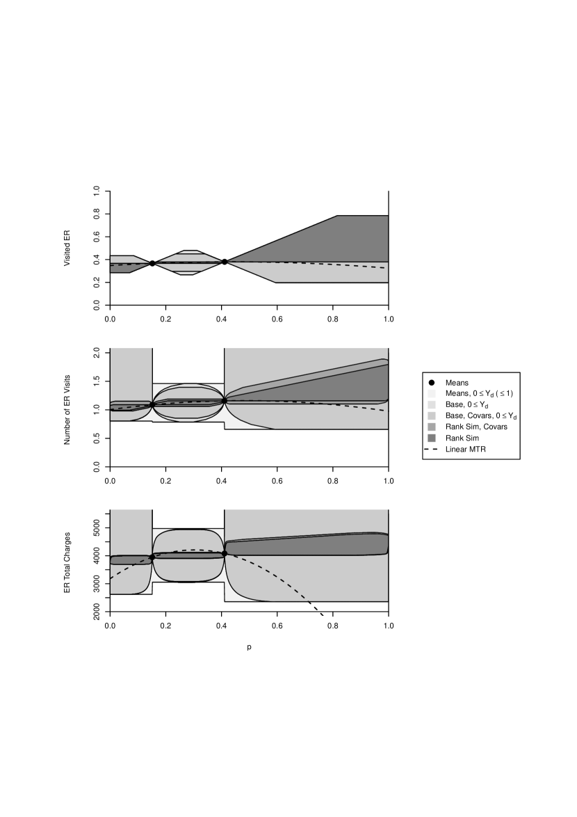
Figure 1: Uniformly Sharp Bounds on Counterfactual Average Outcomes for OHIE Data. This figure empirically implements the uniformly sharp bounds on counterfactual average outcomes of Proposition 1 for the OHIE data across the three ER utilization outcomes: whether a participant visited the ER, the number of ER visits, and the total ER charges incurred. These uniform bounds summarize the empirical content of the (rank similar and/or covariate-conditional) latent index models for the family of (positively) weighted average treatment effects. In particular, bounds for the counterfactual LATE parameters in Table 1 could be derived from the information in this figure. In the case of the binary indicator of whether an experiment subject visited the ER, the mean and distribution bounds coincide because distributions are characterized by their means. In the other cases, incorporating distribution information improves identification, and also allows the researcher to incorporate distribution assumptions, such as rank similarity. The uniform bounds illustrate how the extrapolations based on rank similarity differ substantively from the parametric extrapolation based on means alone.

At the same time, the aim of the preceding comparison is not to argue that rank similarity is necessarily a better assumption than outcome monotonicity or linearity in the OHIE context, but rather to highlight the third contribution: the framework and its incorporation of distribution information allows the researcher to compare the content of various mean and distribution assumptions and assess their joint consistency. As an additional such example, in Figure 1, the MTE function obtained under the linearity assumption for total charges is too dispersed to have been generated by a (conditionally) rank similar data-generating process among compliers. Thus again, the linearity and rank similarity assumptions do not appear jointly consistent. More generally, this shows how distribution information alone could in theory reject functional-form assumptions that point-identify functional parameters of interest, as in Corollary 3. Additionally, the uniform bounds in Figure 1 provide a specification test of unconditional rank similarity, as formalized in Proposition 6. In this case, the visible difference in unconditional and conditional rank similar bounds for the number of ER visits provides some suggestive evidence against unconditional rank similarity for that outcome; however, such evidence is nonexistent for the binary visit outcome and seemingly more limited for the ER total charge outcome. The statistical formalization of these observations is left to future work.

Finally, the preceding insights — as well as the features of data required for sharply bounding all weighted treatment effects $\text{WTE}(w)$ across the different auxiliary assumptions — are compactly summarized in the uniform bounds of Figure 1. Thus the proposed methods provide an overarching framework for the partial identification of treatment effects in the latent index selection model.

6 Conclusion

This paper characterizes the set of feasible MTE functions and derives sharp, analytic bounds on weighted average treatment effects in the latent index selection model [Heckman and Vytlacil [1999, 2005]; Vytlacil [2002]]. The latent index selection model is a popular instrumental-variable framework for identification, which in many empirical settings defines a larger class of parameters than it identifies. For example, in the empirical setting of the Oregon Health Insurance Experiment, the researcher or policymaker may be interested in the effects of charging a price for expanded insurance coverage, or of expanding coverage to an even larger population. A theme of the paper is that sharp characterizations of the latent index selection model’s empirical content fully utilize identified marginal distributions. Furthermore, such distribution information is useful for encoding new auxiliary assumptions into the latent index framework, which may yield quite different predictions than assumptions that use means alone.

There are several interesting possibilities for future work. One is to (sharply) incorporate other auxiliary distribution assumptions into the model. Another is to study whether the analytical expressions for bounds can be used to simplify results about statistical inference. Finally, and most generally, it would be interesting to study how the analytical toolkit and results in this paper could be used to obtain sharp, analytical results in generalized models that relax the binary nature of the treatment decision or the structure of the latent index selection rule.

Appendix A Empirical Table and Figure

Model
Parameter	Means	Base	Covariate	Conditional Rank Sim.	Rank Sim.	Linearity
Panel A. Outcome: Visited ER, Covariate: Visited ER in Pre-Period, $N=$ 19,643
$\text{LATE}(0,\overline{p}_{0})$	$[-0.45,0.55]$	$[-0.45,0.55]$	$[-0.45,0.55]$	$[0,0.55]$	$[0,0.55]$	$\{0.13\}$
$\text{LATE}(\overline{p}_{0},\overline{p}_{1})$	$\{0.05\}$	$\{0.05\}$	$\{0.05\}$	$\{0.05\}$	$\{0.05\}$	$\{0.05\}$
$\text{LATE}(\overline{p}_{1},1)$	$[-0.31,0.69]$	$[-0.31,0.69]$	$[-0.31,0.69]$	$[0,0.69]$	$[0,0.69]$	$\{-0.10\}$
$\text{LATE}(\overline{p}_{0},\overline{p}_{1}-0.1(\overline{p}_{1}-\overline{p}_{0}))$	$[-0.05,0.17]$	$[-0.05,0.17]$	$[-0.06,0.17]$	$[0,0.06]$	$[0,0.06]$	$\{0.06\}$
$\text{LATE}(\overline{p}_{0},\overline{p}_{1}+0.1(\overline{p}_{1}-\overline{p}_{0}))$	$[-0.04,0.14]$	$[-0.04,0.14]$	$[-0.05,0.14]$	$[0.05,0.14]$	$[0.05,0.14]$	$\{0.05\}$
$\text{LATE}(0,1)$	$[-0.24,0.50]$	$[-0.24,0.50]$	$[-0.24,0.50]$	$[0.01,0.50]$	$[0.01,0.50]$	$\{-0.02\}$
Panel B. Outcome: Number of ER Visits, Covariate: Number of ER Visits in Pre-Period (Truncated at 10), $N=$ 19,615
$\text{LATE}(0,\overline{p}_{0})$	$(-\infty,1.88]$	$(-\infty,1.88]$	$(-\infty,1.88]$	$[-0.18,0.44]$	$[0.12,0.63]$	$\{0.55\}$
$\text{LATE}(\overline{p}_{0},\overline{p}_{1})$	$\{0.27\}$	$\{0.27\}$	$\{0.28\}$	$\{0.28\}$	$\{0.27\}$	$\{0.27\}$
$\text{LATE}(\overline{p}_{1},1)$	$[-0.85,\infty)$	$[-0.85,\infty)$	$[-0.85,\infty)$	$[0.06,1.17]$	$[0.07,1.08]$	$\{-0.31\}$
$\text{LATE}(\overline{p}_{0},\overline{p}_{1}-0.1(\overline{p}_{1}-\overline{p}_{0}))$	$[-1.30,1.60]$	$[-0.66,1.11]$	$[-0.53,0.98]$	$[0.00,0.43]$	$[0.13,0.30]$	$\{0.29\}$
$\text{LATE}(\overline{p}_{0},\overline{p}_{1}+0.1(\overline{p}_{1}-\overline{p}_{0}))$	$[-1.51,\infty)$	$[-0.56,\infty)$	$[-0.56,\infty)$	$[0.06,0.79]$	$[0.25,0.51]$	$\{0.25\}$
$\text{LATE}(0,1)$	$(-\infty,\infty)$	$(-\infty,\infty)$	$(-\infty,\infty)$	$[0.08,0.83]$	$[0.13,0.80]$	$\{-0.03\}$
Panel C. Outcome: ER Total Charges, Covariate: Upper Quintile of ER Total Charges in Pre-Period, $N=$ 19,619
$\text{LATE}(0,\overline{p}_{0})$	$(-\infty,8777]$	$(-\infty,8777]$	$(-\infty,8773]$	$[813,1274]$	$[1148,1517]$	$\{5082\}$
$\text{LATE}(\overline{p}_{0},\overline{p}_{1})$	$\{516\}$	$\{436\}$	$\{466\}$	$\{466\}$	$\{437\}$	$\{516\}$
$\text{LATE}(\overline{p}_{1},1)$	$[-2929,\infty)$	$[-2932,\infty)$	$[-2933,\infty)$	$[598,1153]$	$[562,1092]$	$\{-8916\}$
$\text{LATE}(\overline{p}_{0},\overline{p}_{1}-0.1(\overline{p}_{1}-\overline{p}_{0}))$	$[-3828,4402]$	$[-2981,3523]$	$[-2948,3531]$	$[-152,721]$	$[-100,651]$	$\{804\}$
$\text{LATE}(\overline{p}_{0},\overline{p}_{1}+0.1(\overline{p}_{1}-\overline{p}_{0}))$	$[-5579,\infty)$	$[-3824,\infty)$	$[-3797,\infty)$	$[223,2036]$	$[217,1831]$	$\{228\}$
$\text{LATE}(0,1)$	$(-\infty,\infty)$	$(-\infty,\infty)$	$(-\infty,\infty)$	$[596,993]$	$[618,986]$	$\{-4350\}$

Table 1: Sharp Bounds for Various Counterfactual LATE Parameters, OHIE Data. This table provides point estimates of sharp bounds for selected counterfactual LATE parameters discussed in the text across different model specifications for three ER utilization outcomes: whether a participant visited the ER, the number of ER visits, and the total ER charges incurred. Each model is estimated on all observations with non-missing outcome and covariate values. Point-identifying bounds are denoted in brackets. Finally, some discrepancies in point estimates arise because the complier means in the distribution models are derived from estimates of the entire complier outcome distributions; in the case of the highly dispersed total charges outcomes, this leads the mean estimate to be highly dependent on the estimate of the distributions’ extreme right tails.

Appendix B Proofs

Proof of Theorem 1.

To establish necessity, observe that the definition of the MTE function and the group-conditional random vector implies that $\text{MTE}(U_{g})=\mathds{E}[\Delta_{g}|U_{g}]$ for all $g\in\{a,c,n\}$. Then mean consistency (11) follows from the law of total expectation:

$$\mathds{E}[\text{MTE}(U_{g})]=\mathds{E}[\mathds{E}[\Delta_{g}|U_{g}]]=\mathds{E}[\Delta_{g}].$$

For $g=c$, the last term is equal to $\text{LATE}_{IA}$. For distribution consistency, Jensen’s inequality and the law of total expectation imply:

$$\mathds{E}[\phi(\text{MTE}(U_{g}))] =\mathds{E}[\phi(\mathds{E}[\Delta_{g}|U_{g}])]$$

$$\geq\mathds{E}[\mathds{E}[\phi(\Delta_{g})|U_{g}]]$$

$$=\mathds{E}[\phi(\Delta_{g})]$$

for any concave $\phi:\mathds{R}\to\mathds{R}$. Thus $\text{MTE}(U_{g})\succeq_{SSD}\Delta_{g}$ follows by an equivalent and common characterization of SSD dominance, namely (weakly) higher expectations over all increasing concave functions. Additionally,

$$I_{\Delta_{g}}(q)\geq\int_{0}^{q}[Q_{Y_{1,g}}(s)-Q_{Y_{0,g}}(1-s)]\,ds=I_{\Delta_{g}^{-}}(q)\quad\text{for all $q\in[0,1]$.}$$

The inequality follows by definition of the treatment effect, $\Delta_{g}=Y_{1,g}-Y_{0,g}$, whose integral of the lowest $q$ values is at least as high as the lowest $q$ values of $Y_{1,g}$ and the highest $q$ values of $Y_{0,g}$; the equality follows by definition (10) of $\Delta_{g}^{-}$ and the IQF. Thus $\Delta_{g}\succeq_{SSD}\Delta_{g}^{-}$ by definition. Since the SSD order is transitive, combining results yields $\text{MTE}(U_{g})\succeq_{SSD}\Delta_{g}^{-}$. This is an empirical restriction for compliers $g=c$ since the distribution of $\Delta_{c}^{-}$ is recovered from the identified marginals of $Y_{0,c}$ and $Y_{1,c}$.

In contrast, no meaningful restrictions on the MTE function are possible for non-compliers $g\neq c$ because either the conditional distribution of treated or untreated outcomes is unidentified (Lemma 1). By definition of the MTE function (2) and by Lemma 1, the sharp set $\mathcal{M}^{*}$ is equal to the set of integrable functions $m$ that satisfy:

$$m(\hat{U}_{g})=\mathds{E}[\hat{Y}_{1,g}-\hat{Y}_{0,g}|\hat{U}_{g}]$$ (39)

for some random vector $(\hat{U}_{g},\hat{Y}_{0,g},\hat{Y}_{1,g})$ consistent with identified marginals, for every $g\in\{a,c,n\}$. However, for any integrable function $m$ and, say, the always-treated $g=n$, we can choose a conditional joint distribution of $(\hat{U}_{n},\hat{Y}_{0,n},\hat{Y}_{1,n})$ that is consistent with the identified marginals of $U_{n}$ and $Y_{0,n}$ and that satisfies (39); namely, choose the unidentified treated outcome distribution among the never-treated to satisfy $\mathds{E}[\hat{Y}_{1,n}|\hat{U}_{n}]=m(\hat{U}_{n})+\mathds{E}[\hat{Y}_{0,n}|\hat{U}_{n}]$ for any data-consistent $(\hat{U}_{n},\hat{Y}_{0,n})$. Analogous reasoning excludes the possibility of restricting the MTE function on the interval of the always-treated.

To establish sufficiency, it therefore remains to show that if an integrable function $m$ satisfies (11) and (12), there exists a random vector $(\hat{U}_{c},\hat{\Delta}_{c}=\hat{Y}_{1,c}-\hat{Y}_{0,c})$ consistent with the identified marginals of $U_{c}$, $Y_{0,c}$, and $Y_{1,c}$ such that (39) holds. Conditions (11) and (12) are jointly equivalent to (reverse) stochastic dominance in the convex order:

$$m(U_{c})\preceq_{cx}\Delta_{c}^{-}.$$ (40)

In turn, dominance in the convex order is equivalent to the existence of random variables $\hat{M}_{c}$ and $\hat{\Delta}_{c}^{-}$, defined on the same probability space and with marginal distributions equal to those of their namesakes, such that the random vector $(\hat{M}_{c},\hat{\Delta}_{c}^{-})$ is a martingale:

$$\mathds{E}[\hat{\Delta}_{c}^{-}|\hat{M}_{c}]=\hat{M}_{c}.$$

In other words, letting $\mathcal{B}$ denote the Borel $\sigma$-algebra on $\mathds{R}$, dominance in the convex order guarantees the existence of a Markov kernel $\kappa:\mathcal{B}\times\mathds{R}\to[0,1]$ with:

$$\int t\kappa(dt,x)=x\quad\text{for all $x\in\mathds{R}$}$$

and $P_{\Delta_{c}^{-}}(B)=\int\kappa(B,x)\,P_{m(U_{c})}(dx)$ for all $B\in\mathcal{B}$. But then the joint distribution generated by a $\hat{U}_{c}$ with the marginal distribution of $U_{c}$ and the conditional law $[\hat{\Delta}_{c}^{-}|\hat{U}_{c}=u]$ corresponding to $\kappa(\cdot,m(u))$ yields a joint distribution with empirically consistent marginals satisfying:

$$\mathds{E}[\hat{\Delta}_{c}^{-}|\hat{U}_{c}]=m(\hat{U}_{c}).$$

This is the desired result.

Finally, to show that the sharp set $\mathcal{M}^{*}$ is convex, consider elements $m,m^{\prime}\in\mathcal{M}^{*}$ with corresponding complier kernels $\kappa,\kappa^{\prime}$. Then for any $\alpha\in[0,1]$, the joint distribution generated by a $\tilde{U}_{c}$ with the marginal distribution of $U_{c}$ and the conditional law $[\tilde{\Delta}_{c}^{-}|\tilde{U}_{c}=u]$ corresponding to the mixture $\alpha\kappa(\cdot,m(u))+(1-\alpha)\kappa^{\prime}(\cdot,m^{\prime}(u))$ yields a joint distribution with empirically consistent marginals satisfying:

$$\mathds{E}[\tilde{\Delta}_{c}^{-}|\tilde{U}_{c}]=\alpha m(\tilde{U}_{c})+(1-\alpha)m^{\prime}(\tilde{U}_{c})$$

Since $\alpha m+(1-\alpha)m^{\prime}$ also inherits integrability, it follows that the function belongs to $\mathcal{M}^{*}$.

∎

Proof of Theorem 2.

In the basic formulation (Assumption 1 and Assumption 2), a necessary condition for finite bounds on WTE$(w)$ is that weights are nonzero only among compliers:

$$P(w(U)\neq 0,G\neq c)=0.$$ (41)

Else, suppose $P(w(U)>0,G\neq c)>0$, and let $\mathcal{U}_{-c,+}=\{u:w(u)>0,u\notin[\overline{p}_{0},\overline{p}_{1}]\}$. (The case where $w$ is instead negative follows analogously.) For any candidate finite upper (analogously, lower) bound $k\in\mathds{R}$ we can construct a violation as follows. Consider the family of candidate MTE functions:

$$m_{n}(u)=\begin{cases}n&\text{if $u\in\mathcal{U}_{-c,+}$}\\ \text{LATE}(\overline{p}_{0},\overline{p}_{1})&\text{if $u\notin\mathcal{U}_{-c,+}$ }\end{cases}$$

which by Theorem 1 belongs to $\mathcal{M}^{*}$ for any $n\in\mathds{N}$. Yet for:

$$n_{k}>\frac{k-\text{LATE}(\overline{p}_{0},\overline{p}_{1})E[w(U)\mathds{I}\{U\notin\mathcal{U}_{-c,+}\}]}{E[w(U)\mathds{I}\{U\in\mathcal{U}_{+,-c}\}]}$$

we have that $\int m_{n_{k}}(u)w(u)\,du>k$, yielding a violation of the supposed bound. Thus, no finite bounds on such $\text{WTE}(w)$ exist, and it suffices to consider $\text{WTE}(w)$ where (41) holds and to specify functions that extremize $\text{WTE}(w)$ on the interval of compliers.

Fix $w$ and consider an $\overline{m}_{w}$ satisfying (15). Fix any other $m\in\mathcal{M}^{*}$, and to simplify notation let $M=m(U_{c})$, $W=w(U_{c})$, and $\bar{M}=\overline{m}_{w}(U_{c})$, and $V\sim U[0,1]$. Then:

$$\frac{1}{P(G=c)}\int_{\overline{p}_{0}}^{\overline{p}_{1}}m(u)w(u)\,du =\mathds{E}[MW]$$ (42)

$$\leq\mathds{E}[Q_{M}(V)Q_{W}(V)]$$ (43)

$$\leq\mathds{E}[Q_{\Delta_{c}^{-}}(V)Q_{W}(V)]$$ (44)

$$=\mathds{E}[\bar{M}W]=\frac{1}{P(G=c)}\int_{\overline{p}_{0}}^{\overline{p}_{1}}\overline{m}_{w}(u)w(u)\,du$$ (45)

The equality in (42) follows by definition of the random variables. The inequality (43) follows from Theorem 9.A.21 of Shaked and Shantikumar [2007] and the fact that $f(x,y)=xy$ is a supermodular function. Note that $(Q_{M}(V),Q_{W}(V))$ is the joint distribution where $M$ and $W$ are comonotonic, i.e. exhibit perfect positive dependence. Inequality (44) follows from Theorem 3.A.9 of Shaked and Shantikumar [2007], the sharp set characterization of Theorem 1, and the fact that $Q_{W}(\cdot)$ is a nondecreasing function. Finally, equality (45) follows from the assumed properties in (15), which impose comonotonicity between the extremal MTE function and the weights. An analogous argument holds for the function $\underline{m}_{w}$ attaining the lower bound by working with the negative weight $-w$. ∎

Proof of Proposition 1.

Combining (17) with the identification of $\bar{y}(\overline{p}_{z})=\mathds{E}[Y|Z=z]$, a function $a:[0,1]\to\mathds{R}$ is a counterfactual outcome candidate function if and only if it has a representation:

$$a(p)=\bar{y}(\overline{p}_{0})+\int_{\overline{p}_{0}}^{p}m(u)\,du$$ (46)

for some marginal treatment effect candidate $m\in\mathcal{M}^{*}$. Thus any candidate outcome function $a$ is absolutely continuous, with $a(\overline{p}_{0})=\bar{y}(\overline{p}_{0})$ and derivative $a^{\prime}=m$ almost everywhere, i.e. $a^{\prime}\in\mathcal{M}^{*}$. I proceed to show necessity and sufficiency of (19).

Necessity: The upper bound of (19) must be satisfied by virtue of a decreasing rearrangement and the pointwise upper bound of Corollary 2:

$$a(\overline{p}_{0})+\int_{\overline{p}_{0}}^{p}(a^{\prime})^{\uparrow_{c}}(u)\,du\leq a(p)\leq\psi_{h}(p)$$

For the lower bound, restricting for simplicity of notation to the complier interval $p\in[\overline{p}_{0},\overline{p}_{1}]$ where the pointwise bounds are meaningful,

$$a(\overline{p}_{0})+\int_{\overline{p}_{0}}^{p}(a^{\prime})^{\uparrow_{c}}(u)\,du =a(\overline{p}_{0})+\int_{\overline{p}_{0}}^{p}Q_{a^{\prime}(U_{c})}\left(\frac{u-\overline{p}_{0}}{\overline{p}_{1}-\overline{p}_{0}}\right)\,du$$

$$=a(\overline{p}_{0})+(\overline{p}_{1}-\overline{p}_{0})\cdot I_{a^{\prime}(U_{c})}\left(\frac{p-\overline{p}_{0}}{\overline{p}_{1}-\overline{p}_{0}}\right)$$

$$\geq\bar{y}(\overline{p}_{0})+(\overline{p}_{1}-\overline{p}_{0})\cdot I_{\Delta_{c}^{-}}\left(\frac{p-\overline{p}_{0}}{\overline{p}_{1}-\overline{p}_{0}}\right)=\psi_{l}(p).$$

The inequality follows because $a(\overline{p}_{0})=\bar{y}(\overline{p}_{0})$ and $a^{\prime}\in\mathcal{M}^{*}$, and therefore $I_{a^{\prime}(U_{c})}(q)\geq I_{\Delta_{c}^{-}}(q)$ pointwise by (12) and the definition of SSD.

Sufficiency: Fix an absolutely continuous $a:[0,1]\to\mathds{R}$, which by definition is differentiable almost everywhere and has a representation:

$$a(p)=a(\overline{p}_{0})+\int_{\overline{p}_{0}}^{p}a^{\prime}(u)\,du.$$

where the derivative $a^{\prime}$ is integrable. Suppose furthermore that the rearrangement of $a$ satisfies (19). Evaluated at $p=\overline{p}_{0}$, the pointwise bounds imply:

$$a(\overline{p}_{0})=\bar{y}(\overline{p}_{0})=\psi_{l}(\overline{p}_{0})=\psi_{u}(\overline{p}_{0}).$$ (47)

Evaluated at $p\in[\overline{p}_{0},\overline{p}_{1}]$, the (lower) bounds imply:

$$I_{a^{\prime}(U_{c})}\left(\frac{p-\overline{p}_{0}}{\overline{p}_{1}-\overline{p}_{0}}\right)\geq I_{\Delta_{c}^{-}}\left(\frac{p-\overline{p}_{0}}{\overline{p}_{1}-\overline{p}_{0}}\right)\quad\text{for $p\in[\overline{p}_{0},\overline{p}_{1}]$}$$ (48)

This follows from plugging in $a(\overline{p}_{0})=\bar{y}(\overline{p}_{0})$ and recalling that:

$$\int_{\overline{p}_{0}}^{p}(a^{\prime})^{\uparrow_{c}}(u)\,du=(\overline{p}_{1}-\overline{p}_{0})\cdot I_{a^{\prime}(U_{c})}\left(\frac{p-\overline{p}_{0}}{\overline{p}_{1}-\overline{p}_{0}}\right)\quad\text{for $p\in[\overline{p}_{0},\overline{p}_{1}]$.}$$

Finally, evaluated at $p=\overline{p}_{1}$, the bounds imply:

$$I_{a^{\prime}(U_{c})}(1)=\mathds{E}[a^{\prime}(U_{c})]=\text{LATE}_{IA}.$$ (49)

Combining (48), (49), and integrability implies that $a^{\prime}\in\mathcal{M}^{*}$ by Theorem 1. Combining $a^{\prime}\in\mathcal{M}^{*}$ with (47) yields the sufficient representation (46), and so $a\in\mathcal{A}^{*}$. Finally, convexity follows from the sufficient representation (46) and convexity of the set $\mathcal{M}^{*}$.

∎

Appendix C Remaining Proofs (Online Appendix)

Proof of Lemma 1.

From the definition (9) and the latent index formulation (1), the groups are equivalently expressed in terms of unobservables: $\{G=a\}=\{U\leq\overline{p}_{0}\}$, $\{G=c\}=\{\overline{p}_{0}<U\leq\overline{p}_{1}\}$, and $\{G=n\}=\{\overline{p}_{1}<U\}$. Therefore the group probabilities are given by $P(G=a)=\overline{p}_{0}$, $P(G=c)=\overline{p}_{1}-\overline{p}_{0}$, and $P(G=n)=1-\overline{p}_{1}$, and Bayes’ rule implies that the conditional $U_{g}$ are uniformly distributed on their respective supports.

The observed distribution of $(D,Y,Z)$ is equivalently expressed as the probabilities $P(D=d,Z=z)$ and the conditional outcome cdfs $F_{Y|D=d,Z=z}=F_{Y_{d}|D=d,Z=z}$ for all $(d,z)\in\{0,1\}^{2}$. Consider a partition of the sample space $\Omega$ into the observed sets $\{D=d,Z=z\}$. Since $D=1$ implies $G\in\{a,c\}$ and $D=0$ implies $G\in\{c,n\}$, a weakly finer partition than the sets $\{D=d,Z=z\}$ is given by the sets $\{G=g,Z=z\}$. Furthermore, $\{D=1,Z=0\}=\{D_{0}=1,Z=0\}=\{G=a,Z=0\}$. Next, the earlier expression of $G$ as a function of $U$ combined with independence $U\perp Z$ imply that $G\perp Z$. Thus $\{G=a,Z=0\}$ is a random subset of $\{G=a\}$, for which $Y_{1}$ is observed. Therefore $F_{Y_{1,a}}(y)=F_{Y|D=1,Z=0}(y)$. By analogous reasoning, $F_{Y_{0,n}}(y)=F_{Y|D=0,Z=1}(y)$. For compliers $G=c$, Imbens and Rubin [1997] show that the distributions of compliers outcomes $Y_{d,c}$ are identified for both treatment decisions $d\in\{0,1\}$; see also Abadie [2002] for an expression of the complier outcome cdfs as a function of the data.

Conversely, observe that within each group $\{G=g,Z=z\}$, at most one potential outcome $Y_{d}$ (or rather, its distribution) is observed, while any information on the other $Y_{1-d}$ is recovered by independence of $G$ and $Z$. Therefore the data and model impose no assumptions beyond consistency with the identified marginals on the conditional joint distribution of $Y_{0}$ and $Y_{1}$ within each set $\{G=g\}$. Since the partition into sets $\{U=u\}$ is finer than the partition into $\{G=g\}$, the result holds also for the conditional joint distribution of $(U,Y_{0},Y_{1})$ within each set $\{G=g\}$. Thus any joint distribution consistent with the identified conditional marginals can be generated in a way that is consistent with the model and the data.

∎

Proof of Proposition 2.

The proof follows from algebra and definitions:

$$R(\overline{p}_{0},\overline{p}_{1}) =\int_{\overline{p}_{0}}^{\overline{p}_{1}}[\psi_{h}(u)-\psi_{l}(u)]\,du$$

$$=(\overline{p}_{1}-\overline{p}_{0})\int_{0}^{1}\left[\psi_{h}(\overline{p}_{0}+(\overline{p}_{1}-\overline{p}_{0})q)-\psi_{l}(\overline{p}_{0}+(\overline{p}_{1}-\overline{p}_{0})q)\right]\,dq$$

$$=(\overline{p}_{1}-\overline{p}_{0})\int_{0}^{1}\left[\bar{y}(\overline{p}_{1})-\bar{y}(\overline{p}_{0})-(\overline{p}_{1}-\overline{p}_{0})[I_{\Delta_{c}^{-}}(1-q)+I_{\Delta_{c}^{-}}(q)]\right]\,dq$$

$$=(\overline{p}_{1}-\overline{p}_{0})^{2}\int_{0}^{1}\left[\text{LATE}_{IA}-2I_{\Delta_{c}^{-}}(q)\right]\,dq$$

$$=(\overline{p}_{1}-\overline{p}_{0})^{2}\cdot 2\int_{0}^{1}\left[q\cdot\text{LATE}_{IA}-I_{\Delta_{c}^{-}}(q)\right]\,dq$$

$$=(\overline{p}_{1}-\overline{p}_{0})^{2}\cdot\Gamma_{\Delta_{c}^{-}}$$

∎

Proof of Proposition 3.

It suffices to show that $\text{MTE}(U_{g})=\mathds{E}[\Delta_{g}^{+}|U_{g}]$ for each $g\in\{a,c,n\}$, at which point necessity of the conditions follows by the same reasoning as in the necessity proof of Theorem 1. Observe:

$$\text{MTE}(U_{g}) =\mathds{E}[Y_{1,g}-Y_{0,g}|U_{g}]$$

$$=\mathds{E}[Q_{Y_{1}}(V_{1,g})-Q_{Y_{0}}(V_{0,g})|U_{g}]$$

$$=\mathds{E}[Q_{Y_{1}}(V_{0,g})-Q_{Y_{0}}(V_{0,g})|U_{g}]$$

$$=\mathds{E}[\Delta_{g}^{+}|U_{g}]$$

where the first equality follows by definition of the MTE function and the group-conditional random vector, the second equality by the Skorokhod representation implicit in the definition of rank similarity, the third equality by rank similarity, and the last equality by definition of $\Delta_{g}^{+}$. ∎

Proof of Lemma 2.

The result is proved for realizations of $U$, from which it follows for any function thereof, i.e. random variables measurable with respect to $U$. Let $QQ_{u}$ denote the conditional $QQ$ plot for $U=u$. By the Skorokhod quantile representation implicit in the assumption of rank similarity, the conditional quantile function of outcomes is equal to the unconditional quantile function of outcomes evaluated at the conditional quantile function of ranks. That is, letting $Y_{d,u}\sim Y_{d}|U=u$ and $V_{d,u}\sim V_{d}|U=u$,

$$Q_{Y_{d,u}}(q)=Q_{Y_{d}}(Q_{V_{d,u}}(q))\quad\text{for all $q,u\in[0,1]$.}$$

By rank similarity, the conditional distribution of rank variables are equal. Expressed in terms of the quantile functions,

$$Q_{V_{0,u}}(q)=Q_{V_{1,u}}(q)\quad\text{for all $q,u\in[0,1]$.}$$

Combining these observations yields the desired result:

$$QQ_{u} =\{(Q_{Y_{0,u}}(q),Q_{Y_{1,u}}(q)):q\in[0,1]\}$$

$$=\{Q_{Y_{0}}(Q_{V_{0,u}}(q)),Q_{Y_{1}}(Q_{V_{1,u}}(q)):q\in[0,1]\}$$

$$=\{Q_{Y_{0}}(Q_{V_{0,u}}(q)),Q_{Y_{1}}(Q_{V_{0,u}}(q)):q\in[0,1]\}\subseteq QQ.$$

∎

Proof of Lemma 3.

Lemma 2 implies that $QQ_{g}\subseteq QQ$ for all $g\in\{a,c,n\}$. Assumption 5 implies that $QQ=QQ_{c}$, and so $QQ_{g}\subseteq QQ_{c}$. Necessity of the bounds then follows by definition.

To prove uniform sharpness for $(d,g)\in\{(0,a),(1,n)\}$, note first that the bounds are identified from the data because the quantile function $Q_{Y_{1-d,g}}$ is identified in the basic model (Assumption 1 and Assumption 2). It remains to show that the bounds are attained by a data-generating process consistent with the assumptions. For any bound, consider a rank-invariant Skorokhod representation, e.g. $(Y_{0,n},Y_{1,n})\stackrel{{\scriptstyle d}}{{=}}(Q_{Y_{0,n}}(V),\underline{Q}_{Y_{1,n}}(V))$ for $V\sim U[0,1]$. This satisfies the basic model, which imposed no restrictions on the extrapolated quantile function. Additionally, its quantile-quantile plot belongs to the true population plot $QQ$ by construction of the extrapolated quantile function, Lemma 2, and the closed complete support condition of Assumption 5. This guarantees that the rank invariant construction by group $g$ is also rank-invariant in the population, and thus satisfies (either version of) Assumption 4. ∎

Proof of Proposition 4.

As in the proof of Theorem 2, fix $w$, consider an $\overline{m}_{w}$ satisfying (35), and for consistency of notation let $M_{g}=m(U_{g})$, $W_{g}=w(U_{g})$, $\bar{M}_{g}=\overline{m}_{w}(U_{g})$, and $V\sim U[0,1]$.

Suppose momentarily that the distribution of each $\Delta_{g}^{+}$ were identified. In that case, following the logic of Theorem 1, the necessary characterization of Proposition 3 becomes sufficient for characterizing the set $\mathcal{M}^{+}$ of empirically consistent MTE functions under the additional Assumption 4 and Assumption 5. Then the desired result follows analogously to the proof of Theorem 2 upon decomposing the functional into its group conditional components:

$$\int_{0}^{1}m(u)w(u)\,du=\sum_{g}\mathds{E}[M_{g}W_{g}]\cdot P(G=g),$$

and maximizing piecewise. Namely, analogous reasoning to the proof of Theorem 2 yields:

$$\int_{0}^{1}m(u)w(u)\,du\leq\sum_{g}\mathds{E}[Q_{\Delta_{g}^{+}}(V)Q_{W_{g}}(V)]\cdot P(G=g)$$

Now consider the case where the distribution of $\Delta_{g}^{+}$ is not fully identified, but rather bounded by Lemma 4, i.e. $\Delta_{g}^{+}\preceq_{FSD}\overline{\Delta}_{g}^{+}$. By assumption, $w(u)\geq 0$ for all $u$, so that also $Q_{W_{g}}(V)\geq 0$. Combining these observations, it follows that:

$$\mathds{E}[Q_{\Delta_{g}^{+}}(V)Q_{W_{g}}(V)]\leq\mathds{E}[Q_{\overline{\Delta}_{g}^{+}}(V)Q_{W_{g}}(V)]$$

for each $g$. By definition of $\overline{m}_{w}$, the right hand side is equal to $\mathds{E}[\overline{M}_{g}W_{g}]$ for each $g$, and so:

$$\int_{0}^{1}m(u)w(u)\,du\leq\int_{0}^{1}\overline{m}_{w}(u)w(u)\,du$$

for all $m\in\mathcal{M}^{+}$. Finally, the underlying group-conditional treatment effects $\overline{\Delta}_{g}^{+}$ are jointly attainable by Lemma 4, which proves the sharpness of the upper bound. An argument for the lower bound follows analogously. ∎

Proof of Proposition 5.

First, it will be useful to observe that the “reverse” integrated quantile function, which aggregates quantiles in decreasing order, can be expressed as:

$$\int_{q}^{1}Q_{X}(v)\,dv=\mathds{E}[X]-I_{X}(q)$$ (50)

for any integrable $X$ and $q\in[0,1]$ because $\int_{0}^{1}Q_{X}(v)\,dv=\mathds{E}[X]$.

Combining Proposition 3 and Lemma 4 implies:

$$I_{\text{MTE}(U_{g})}(q)\geq I_{\Delta_{g}^{+}}(q)\geq I_{\underline{\Delta}_{g}^{+}}(q)$$ (51)

for all $q\in[0,1]$, by definition of SSD and the fact that FSD is a stronger ordering (i.e. FSD implies SSD). Additionally, the combination of aforementioned results implies:

$$\mathds{E}[\text{MTE}(U_{g})]-I_{\text{MTE}(U_{g})}(q)\leq\mathds{E}[\Delta_{g}^{+}]-I_{\Delta_{g}^{+}}(q)\leq\mathds{E}[\overline{\Delta}_{g}^{+}]-I_{\overline{\Delta}_{g}^{+}}(q)$$ (52)

The first inequality follows from equality of means and SSD; by (50), the second inequality is equivalent to:

$$\int_{q}^{1}Q_{\Delta_{g}^{+}}(v)\,dv\leq\int_{q}^{1}Q_{\overline{\Delta}_{g}^{+}}(v)\,dv$$

which follows from FSD.

Now consider parameter values among the always-treated, i.e. $p\in[0,\overline{p}_{0}]$. By virtue of increasing and decreasing rearrangements it must be that:

$$\int_{p}^{\overline{p}_{0}}Q_{\text{MTE}(U_{a})}\left(\frac{\overline{p}_{0}-u}{\overline{p}_{0}}\right)\,du\leq\int_{p}^{\overline{p}_{0}}\text{MTE}(u)\,du\leq\int_{p}^{\overline{p}_{0}}Q_{\text{MTE}(U_{a})}\left(\frac{u}{\overline{p}_{0}}\right)\,du$$

Equivalently, by a change of variables and invoking (50),

$$\overline{p}_{0}\cdot I_{\text{MTE}(U_{a})}\left(\frac{\overline{p}_{0}-p}{\overline{p}_{0}}\right)\leq\int_{p}^{\overline{p}_{0}}\text{MTE}(u)\,du \leq\overline{p}_{0}\cdot\left[\mathds{E}[\text{MTE}(U_{a})]-I_{\text{MTE}(U_{a})}\left(\frac{p}{\overline{p}_{0}}\right)\right]$$

Then invoking the inequalities (51) and (52) implies:

$$\overline{p}_{0}\cdot I_{\underline{\Delta}_{a}^{+}}\left(\frac{\overline{p}_{0}-p}{\overline{p}_{0}}\right)\leq\int_{p}^{\overline{p}_{0}}\text{MTE}(u)\,du \leq\overline{p}_{0}\cdot\left[\mathds{E}[\overline{\Delta}_{a}^{+}]-I_{\overline{\Delta}_{a}^{+}}\left(\frac{p}{\overline{p}_{0}}\right)\right]$$

Combining these bounds with the fact that $\bar{y}(p)=\bar{y}(\overline{p}_{0})-\int_{p}^{\overline{p}_{0}}\text{MTE}(u)\,du$ then yields the desired result among the always-treated, $p\in[0,\overline{p}_{0}]$. Analogous reasoning yields the bounds among the never-treated, $p\in[\overline{p}_{1},1]$. The complier bounds are similarly obtained but invoke the stronger inequalities in (51) and (52). Finally, uniform sharpness of these bounds follows from Lemma 4.

∎

Proof of Proposition 6.

To rank the assumptions, suppose the strong version (Assumption 6b) holds, and let $V_{d,x}\sim(V_{d}|X=x)$ and $\tilde{V}_{d}=F_{V_{d,X}}(V_{d})$. Such $\tilde{V}_{d}$ are identically distributed conditional on $(X,U)=(x,u)$ because $V_{0}$ and $V_{1}$ are conditionally identically distributed, which further implies $F_{V_{0,x}}(\cdot)=F_{V_{1,x}}(\cdot)$. Additionally, using the Skorokhod representation’s implication that $Q_{Y_{d,x}}(q)=Q_{Y_{d}}(Q_{V_{d,x}}(q))$, it follows that:

$$Q_{Y_{d,X}}(\tilde{V}_{d})=Q_{Y_{d}}(Q_{V_{d,X}}(F_{V_{d,X}}(V_{d})))\stackrel{{\scriptstyle a.s.}}{{=}}Q_{Y_{d}}(V_{d})=Y_{d}.$$

Thus $\tilde{V}_{d}$ satisfy Assumption 6a (almost surely). The first testable implication (37) follows immediately from Lemma 2. For the second implication, first note that while the rank random variables $V_{d}$ or $\tilde{V}_{d}$ need not be unique if potential outcomes are not continuous, any possible rank variables induce the same outcomes. Therefore the implication follows immediately from the definition of the respective comonotonic effects and the fact that the strong rank invariance assumption implies the weak version. ∎

Appendix D Relation to Distribution of Treatment Effects (Online Appendix)

This appendix provides a pair of counter-examples illustrating that i) neither the second-order bounds (21) nor ii) the combination of first-order Makarov bounds and second-order bounds characterize the sharp set of treatment effects. In addition, this appendix provides a simple example where the MTE relaxation of the quantile functional bounding problem provides different but still intuitive answers.

First, recall the Makarov [1981] bounds on the sum of two random variables with known marginal distributions, introduced into the treatment effect framework by Fan and Park [2010]. Respectively let $\Delta^{L}$ and $\Delta^{U}$ be random variables with the following distributions:

$$F_{\Delta^{L}}(\delta) =\sup_{y}\max\{F_{Y_{1}}(y)-F_{Y_{0}}(y-\delta),0\}$$

$$F_{\Delta^{U}}(\delta) =1+\inf_{y}\min\{F_{Y_{1}}(y)-F_{Y_{0}}(y-\delta),0\}$$

The Makarov bounds are summarized by the first-order stochastic dominance relation:

$$\Delta^{L}\preceq_{FSD}\Delta\preceq_{FSD}\Delta^{U}$$ (53)

As observed by Fan and Park [2010], (53) provides pointwise sharp bounds on the distribution and quantile functions of the treatment effect $\Delta$.

Neither the first-order stochastic relation (53) nor the second-order stochastic relation (21) characterizes the set of possible treatment effects. The first observation is due to Firpo and Ridder [2019], and the second observation is shown by counter-example. A fortiori, I show (again by counter-example) that the combination of first and second-order relations (53) and (21) does not characterize the sharp set of treatment effect distributions.

For the pair of counter-examples, it suffices to consider the case where $P(Y_{d}=y)=1/2$ for $(d,y)\in\{0,1\}^{2}$. In that case, every realized treatment effect belongs to the set $\{-1,0,1\}$. Thus feasible distribution functions $F$ are summarized by their values at three points, $(F(-1),F(0),F(1))$. In fact, the same is true of the distribution functions corresponding to the first-order Makarov bounds $F_{\Delta^{L}}=(0,1/2,1)$ and $F_{\Delta^{U}}=(1/2,1,1)$, as well as the second-order bounds $F_{\Delta^{-}}=(1/2,1/2,1)$ and $F_{\Delta^{+}}=(0,1,1)$. For the second-order bounds, the integrated distribution functions (IDF) $\tilde{I}(\cdot)$ are then given by:

$$\tilde{I}_{\Delta^{+}}(\delta)=\begin{cases}0&\text{for $\delta\in[-1,0)$}\\ \delta&\text{for $\delta\in[0,1]$}\end{cases}\quad\text{and}\quad\tilde{I}_{\Delta^{-}}(\delta)=\frac{\delta+1}{2}\text{ for $\delta\in[-1,1]$.}$$ (54)

For the first counter-example, consider:

$$F_{1}(\delta)=\begin{cases}\frac{1}{3}&\text{for $\delta\in\left[-1,\frac{1}{2}\right)$}\\ 1&\text{for $\delta\in\left[\frac{1}{2},1\right]$}\end{cases}\quad\text{with}\quad\tilde{I}_{1}(\delta)=\begin{cases}\frac{\delta+1}{3}&\text{for $\delta\in\left[-1,\frac{1}{2}\right)$}\\ \delta&\text{for $\delta\in\left[\frac{1}{2},1\right]$}\end{cases}$$

This distribution satisfies the second-order relation (21) because the IDF is pointwise bounded by the extremal IDFs in (54). However, it does not satisfy the necessary first-order Makarov bounds (53). For the second counter-example, consider:

$$F_{2}(\delta)=\begin{cases}0&\text{for $\delta\in\left[-1,-\frac{1}{3}\right)$}\\ \frac{1}{2}&\text{for $\delta\in\left[-\frac{1}{3},\frac{1}{3}\right)$}\\ 1&\text{for $\delta\in\left[\frac{1}{3},1\right]$}\end{cases}\quad\text{with}\quad\tilde{I}_{2}(\delta)=\begin{cases}0&\text{for $\delta\in\left[-1,\frac{1}{3}\right)$}\\ \frac{1}{2}\left[\delta+\frac{1}{3}\right]&\text{for $\delta\in\left[-\frac{1}{3},\frac{1}{3}\right)$}\\ \delta&\text{for $\delta\in\left[\frac{1}{3},1\right]$}\end{cases}$$

This distribution satisfies both the first-order and second-order conditions (53) and (21), but its mass points are not in the set $\{-1,0,1\}$. Therefore it is not a feasible treatment effect distribution.

For the final example, recall from (20) that the Gini coefficient has a simple expression in terms of the quantile function in the case of a nonzero mean. Expressed as a functional $\Phi(\cdot)$ of the quantile function $Q_{\Delta}$,

$$\Phi(Q_{\Delta})=1-\frac{2}{\mathds{E}[\Delta]}\int_{0}^{1}\int_{0}^{q}Q_{\Delta}(u)\,du\,dq$$ (55)

Since the Gini coefficient is a spread parameter in the sense of Stoye [2010], it follows by observation of Fan and Park [2010] that the Gini coefficient of the treatment effect is bounded above and below by (and attains) its values in the extreme cases where the treatment effect is respectively perfectly counter- and co-monotonic. Now consider the relaxed problem of maximizing and minimizing the Gini functional $\Phi(\cdot)$ over feasible MTE functions $m\in\mathcal{M}^{*}$. The relaxed maximization problem still recovers the countermonotonic upper bound; in contrast, the relaxed lower bound is equal to zero, a value attained when marginal treatment effects are homogeneous. Typically this is strictly lower than the lower bound over quantile functions. Nevertheless, the lower bound of zero intuitively captures the minimal amount of ex ante dispersion — that is, dispersion in individuals’ expected (rather than realized) treatment effects. Thus the relaxed lower bound captures an interesting feature, despite differing from the original bound of interest.

References

- 2002 Abadie, A. (2002). “Bootstrap Tests for Distributional Treatment Effects in Instrumental Variable Models.” Journal of the American Statistical Association, 97(457): 284-292.
- 2002 Abadie, A., Angrist, J., and Imbens, G. (2002). “Instrumental Variables Estimates of the Effect of Subsidized Training on the Quantiles of Trainee Earnings.” Econometrica, 70(1): 91-117.
- 1996 Angrist, J.D., Imbens, G.W., and Rubin, D.B. (1996) “Identification of Causal Effects Using Instrumental Variables.” Journal of the American Statistical Association, 91(434): 444-472.
- 1997 Balke, A., and Pearl, J. (1997). “Bounds on Treatment Effects from Studies with Imperfect Compliance.” Journal of the American Statistical Association, 92(439): 1171-1176.
- 1987 Bjorklund, A., and Moffitt, R. (1987). “The Estimation of Wage Gains and Welfare Gains in Self-Selection.” Review of Economics and Statistics, 69(1): 42-49.
- 2017 Brinch, C.N., Mogstad, M., and Wiswall, M. (2017). “Beyond LATE with a Discrete Instrument.” Journal of Political Economy, 125(4): 985-1039.
- 2010 Carneiro, P., Heckman, J.J., and Vytlacil, E.J. (2010). “Estimating Marginal Returns to Education.” American Economic Review, 101: 2754-2781.
- 2011 Carneiro, P., Heckman, J.J., and Vytlacil, E.J. (2011). “Evaluating Marginal Policy Changes and the Average Effect of Treatment for Individuals at the Margin.” Econometrica 78(1): 377-394.
- 2011 Chen, C., Scheffler, G., and Chandra, A. (2011). “Massachusetts’ Health Care Reform and Emergency Department Utilization.” New England Journal of Medicine, 365(12).
- 2010 Chernozhukov, V., Fernández-Val, I., and Galichon, A. (2010). “Quantile and Probability Curves without Crossing.” Econometrica, 78(3): 1093-1125.
- 2005 Chernozhukov, V., and Hansen, C. (2005). “An IV Model of Quantile Treatment Effects.” Econometrica, 73(10): 245-261.
- 1974 Doksum, K. (1974). “Empirical Probability Plots and Statistical Inference for Nonlinear Models in the Two-Sample Case.” Annals of Statistics, 2: 267-277.
- 2018 Dong, Y. and Shen, S. (2018). “Testing for Rank Invariance or Similarity in Program Evaluation.” Review of Economics and Statistics, 100(1): 78-85.
- 2013 Einav, L., Finkelstein, A., Ryan, S.P, Schrimpf, P., and Cullen, M.R. (2013). “Selection on Moral Hazard in Health Insurance.” American Economic Review, 103(1): 178-219.
- 2010 Fan, Y., and Park, S. (2010). “Sharp Bounds on the Distribution of the Treatment Effect and Their Statistical Inference.” Econometric Theory, 26: 931-951.
- 2013 Finkelstein, A. (2013) Oregon Health Insurance Experiment Public Use Data. Available at https://www.nber.org/oregon/1.home.html.
- 2019 Firpo, S. and Ridder, G. (2019). “Partial Identification of the Treatment Effect Distribution and its Functionals.” Journal of Econometrics, 210-234.
- 2018 Frandsen, B.R., and Lefgren, L.J. “Testing Rank Similarity.” Review of Economics and Statistics, 100(1): 86-91.
- 2002 Frangakis, C.E., and Rubin, D.B. (2002). “Principal Stratification in Causal Inference.” Biometrics, 58(1): 21-29.
- 2016 Galichon, A. (2016). Optimal Transport Methods in Economics. Princeton University Press.
- 1971 Gastwirth, J.L. (1971). “A General Definition of the Lorenz Curve.” Econometrica, 39(6): 1037-1039.
- 1929 Hardy, G.H., Littlewood, J.E., and Pólya, G. (1929) “Some Simple Inequalities Satisfied by Convex Functions.” Messenger Math. 58: 145-152.
- 1985 Heckman, J.J., and Robb, R. “Alternative Methods for Evaluating the Impact of Interventions.” (1985). Journal of Econometrics, 30: 239-267.
- 1997 Heckman, J.J., Smith, J., and Clements, N. (1997). “Making the Most Out of Programme Evaluations and Social Experiments Accounting for Heterogeneity in Programme Impacts.” Review of Economic Studies, 64: 487-535.
- 1999 Heckman, J.J. and Vytlacil, E.J. (1999). “Local Instrumental Variables and Latent Variable Models for Identifying and Bounding Treatment Effects.” Proc. Natl. Acad. Sci., 96: 4730-4734.
- 2000 Heckman, J.J. and Vytlacil, E. (2000). “Local Instrumental Variables.” NBER Working Paper No. 252.
- 2001 Heckman, J.J. and Vytlacil, E. (2001). “Policy-Relevant Treatment Effects.” American Economic Review P&P, 91(2): 107-111.
- 2005 Heckman, J.J. and Vytlacil, E. (2005). “Structural Equations, Treatment Efects, and Econometric Policy Evaluation.” Econometrica, 73(3): 669-738.
- 2017 Huber, M., Laffers, L., and Mellace, G. (2017). “Sharp IV Bounds on Average Treatment Effects on the Treated and Other Populations Under Endogeneity and Noncompliance.” Journal of Applied Econometrics, 32: 56-79.
- 1994 Imbens, G.W. and Angrist, J. (1994). “Identification and Estimation of Local Average Treatment Effects.” Econometrica, 62(2): 467-475.
- 1997 Imbens, G.W. and Rubin, D.B. (1997). “Estimating Outcome Distributions for Compliers in Instrumental Variables Models.” Review of Economic Studies, 64(4): 555-574.
- 1989 Jewitt, I. (1989). ”Choosing Between Risky Prospects: The Characterization of Comparative Statics Results, and Location Independent Risk.” Management Science, 35(1): 60-70.
- 2009 Kitagawa, T. “Identification Region of the Potential Outcome Distributions Under Instrument Independence.” Working Paper (2009).
- 2012 Kolstad, J.T., and Kowalski, A.E. (2012). “The Impact of Health Care Reform on Hospital and Preventive Care: Evidence from Massachusetts.” Journal of Public Economics, 96: 909-929.
- 2016 Kowalski, A. (2016). “Doing More When You’re Running LATE: Applying Marginal Treatment Effect Methods to Examine Treatment Effect Heterogeneity in Experiments.” NBER Working Paper 22363.
- 2021 Kowalski, A. (2021). “Reconciling Seemingly Contradictory Results from the Oregon Health Insurance Experiment and the Massachusetts Health Reform.” NBER Working Paper 24647.
- 2019 Kline, P. and Walters, C. (2019). “On Heckits, LATE, and Numerical Equivalence.” Econometrica, 87(2): 677-696.
- 1974 Lehmann, E.L. (1974). Nonparametrics: Statistical Methods Based on Ranks. Holden-Day Inc., San Francisco, CA.
- 2009 Lee, D.S. (2009) “Training, Wages, and Sample Selection: Estimating Sharp Bounds on Treatment Effects.” Review of Economic Studies, 76(3): 1071-1102.
- 1997 Machina, M., and Pratt, J. (1997). “Increasing Risk: Some Direct Constructions.” Journal of Risk and Uncertainty, 14: 103-127.
- 1981 Makarov, G. (1981). “Estimates for the Distribution Function of a Sum of Two Random Variables when the Marginal Distributions are Fixed.” Theory of Probability and its Applications, 26: 803-806.
- 1989 Manski, C.F. (1989). “Anatomy of the Selection Problem.” Journal of Human Resources, 24: 343-360.
- 1990 Manski, C.F. (1990). “Nonparametric Bounds on Treatment Effects.” American Economic Review, Papers and Proceedings, 80(2): 319-323.
- 1994 Manski, C.F. (1994). “The Selection Problem.” In C. Sims, Ed. Advances in Econometrics, Sixth World Congress, Vol 1. Cambridge: Cambridge University Press, p. 143-170.
- 2003 Manski, C.F. (2003). Partial Identification of Probability Distributions. New York: Springer-Verlag.
- 2011 Marshall, A.W., Arnold, B.C., and Olkin, I. (2011). Inequalities: Theory of Majorization and Its Applications. Springer.
- 2019 Marx, P. (2019). “Within Compliers and Beyond: Sharp Bounds in Instrumental Variable Models.” Working Paper.
- 2012 Miller, S. (2012). “The Effect of Insurance on Emergency Room Visits: An Analysis of the 2006 Massachusetts Health Reform.” Journal of Public Economics, 96(11): 893-908.
- 2018 Mogstad, M., Santos, A., and Torgovitsky, A. (2018). “Using Instrumental Variables for Inference About Policy Relevant Treatment Parameters.” Econometrica, 86(5): 1589-1619.
- 1989 Muliere, P., and Scarsini, M. (1989). “A Note on Stochastic Dominance and Inequality Measures.” Journal of Economic Theory, 49(2): 314-323.
- 2018 Mullahy, J. (2018). “Individual Results May Vary: Inequality-Probability Bounds for Some Health-Outcome Treatment Effects.” Journal of Health Economics, 61: 151-162.
- 2001 Müller, A., and Rüschendorf, L. (2001). “On the Optimal Stopping Values Induced by General Dependence Structures.” Journal of Applied Probability, 38(3): 672-684.
- 2002 Ogryczak, W., and Rusczczyński, A. (2002). “Dual Stochastic Dominance and Related Mean-Risk Models.” SIAM Journal of Optimization, 13: 60-78.
- 1970 Rothschild, M., and Stiglitz, J.E. (1970). “Increasing Risk: I. A Definition.” Journal of Economic Theory, 2: 225-243.
- 2007 Shaked, M., and Shanthikumar, J.G. (2007). Stochastic Orders. Springer Science & Business Media.
- 2021 Semenova, V. (2021). “Generalized Lee Bounds.” arXiv preprint arXiv:2008.12720.
- 2011 Smulowitz, P.B., Lipton, R., Wharam, J.F. Adelman, L., Weiner, S.G., Burke, L, Baugh, C.W., Schuur, J.D., Liu, S.W., McGrath, M.E., Liu, B., Sayah, A., Burke, M.C., Pope, J.H., and Landon, B.E. (2011). “Emergency Department Utilization After the Implementation of Massachusetts Health Reform.” Annals of Emergency Medicine, 58(3): 225-234.
- 2010 Stoye, J. (2010). “Partial Identification of Spread Parameters.” Quantitative Economics, 1: 323-357.
- 2014 Taubman, S.L., Allen, H.L., Wright, B.J., Baicker, K., and Finkelstein, A.N. (2014). “Medicaid Increases Emergency-Department Use: Evidence from Oregon’s Health Insurance Experiment.” Science, 343(6168): 263-268.
- 2000 Tian, J. and Pearl, J. (2000). “Probabilities of Causation: Bounds and Identification.” Annals of Mathematics and Artificial Intelligence, 28(1): 287-313.
- 2017 Vuong, Q., and Xu, H. (2017). “Counterfactual Mapping and Individual Treatment Effects in Nonseparable Models with Binary Endogeneity.” Quantitative Economics, 8: 589-610.
- 2002 Vytlacil, E. (2002). “Independence, Monotonicity, and Latent Index Models: An Equivalence Result.” Econometrica, 70(1): 331-341.
- 1991 Williams, D. (1991). “Probability with Martingales.” Cambridge University Press.
- 2003 Zhang, J.L. and Rubin, D.B. (2003). Estimation of Causal Effects via Principal Stratification When Some Outcomes are Truncated by ‘Death.”’ Journal of Educational and Behavioral Statistics, 28(4): 353-368.