Exploiting the scheme dependence of the renormalization group improvement in infrared Yang-Mills theory

Abstract

Within the refined Gribov-Zwanziger scenario for four-dimensional Yang-Mills theory in the Landau gauge, a gluon mass term is generated from the restriction of the gauge field configurations to the first Gribov region. Tissier and Wschebor have pointed out that simply adding a gluon mass term to the usual Faddeev-Popov action yields one-loop renormalization group improved gluon and ghost propagators which are in good agreement with the lattice data even in the infrared regime. In this work, we extend their analysis to several alternative renormalization schemes and show how the renormalization scheme dependence can be used to achieve an almost perfect matching to the lattice data for the gluon and ghost propagators.

I Introduction

Yang-Mills theory, the pure gauge sector of QCD, ows its nontrivial dynamics to the non-Abelian nature of the gauge symmetry, here taken as SU($N$). It is presumably responsible for the peculiar features of the strong interaction such as color confinement and chiral symmetry breaking, which are not present in its Abelian counterpart QED. These phenomena, which are related to the infrared (IR) behavior of the theory and its highly nontrivial vacuum state, are usually considered to be inaccessible to a perturbative approach due to the presence of a Landau pole for the running coupling at the mid-momentum scale $\Lambda_{\text{QCD}}$.

In his seminal paper Gri78 , Gribov showed that the Faddeev-Popov procedure, aimed at fixing the gauge in a covariant way in the non-Abelian case, is valid only perturbatively since for large gauge fields the gauge orbits intersect the gauge-fixing hypersurface in several points (Gribov copies), thus invalidating the Faddeev-Popov construction on a nonperturbative level. In an attempt to overcome the gauge copy ambiguity, Gribov proposed to restrict the functional integration to gauge field configurations for which the Faddeev-Popov operator $(-\partial_{\mu}D_{\mu})$ is positive definite in Euclidean space-time, or, equivalently (in Landau gauge), to local minima of the functional $\int_{x}A^{a}_{\mu}(x)A^{a}_{\mu}(x)$ along the respective gauge orbits Zwa82 ; SF86 , thus defining the (first) Gribov region. Moreover, he was able to show that this restriction of the functional integral avoids the generation of a Landau pole at a nonvanishing scale and changes the behavior of the n-point functions in the IR, which are dominated in this regime by gauge field configurations close to the boundary of the Gribov region footn3 .

For the rest of this paper, we restrict our attention to Yang-Mills theory in the Landau gauge. In the refined Gribov-Zwanziger scenario DGS08 , the possibility of the formation of condensates of the gluon field and various auxiliary fields introduced in order to realize Gribov’s restriction in a local fashion Zwa89 ; Zwa93 , is taken into account. The gluon propagator then develops a massive behavior in the IR, approaching a non-zero value at vanishing momentum. Such an IR finite gluon propagator, together with an IR finite ghost dressing function, corresponds to the decoupling solutions found within the framework of the nonperturbative Dyson-Schwinger equations AN04 ; BBL06 , and also with a mapping to $\lambda\phi^{4}$ theory Fras08 . On the other hand, the scaling solutions of the Dyson-Schwinger equations SHA97 ; SHA98 ; FA02 ; Zwa02 ; LS02 , and also of the functional renormalization group equations PLN04 , are realized when the horizon condition is imposed in the absence of condensates, in which case it amounts to forcing the inverse ghost dressing function to vanish at zero momentum Zwa93 ; Zwa02 .

Perhaps more importantly, the decoupling behavior of the gluon propagator in the IR is in agreement, in three and four space-time dimensions, with Monte Carlo simulations in the minimal Landau gauge on the largest lattices to date BIMS07 ; CM07 ; SSL07 . In the minimal Landau gauge, the restriction to the Gribov region is implemented numerically by selecting, for each gauge orbit, a local minimum of the (appropriately discretized) quadratic functional $\int_{x}A^{a}_{\mu}(x)A^{a}_{\mu}(x)$.

A large body of work has been put together over the years, aiming at an ever more complete and consistent determination of the n-point function of Landau gauge Yang-Mills theory with functional methods. Refs. AP06 ; BLY08 ; HAFS08 ; FMP09 ; AHS10 ; IP13 ; AIP13 ; HS13 ; BHM14 ; EWAV14 ; CHS15 ; ABF16 ; CFM16 ; Hub20 should give an impression of the variety of the approaches and of the sophistication achieved, although our selection of works is inevitably subjective.

In 2010, Tissier and Wschebor TW10 have shown that the lattice results for the gluon and ghost propagators in the IR can be reproduced rather well by plain one-loop calculations with a transverse massive gluon propagator. This massive extension of the Faddeev-Popov action corresponds to a particular case (in the Landau gauge) of a class of massive models originally studied by Curci and Ferrari CF76 with the aim of regularizing the infrared divergences of Yang-Mills theory in a renormalizable way, where the mass parameter was thought to be eventually sent to zero. In our present context, however, the mass parameter is supposed to have a definite non-zero value which is ultimately related to the Gribov parameter that emerges from the restriction to the Gribov region.

One way to understand the appearance of a gluon mass term is from the fact that the restriction of the gauge fields to the Gribov region breaks the nilpotent BRST symmetry of the Faddeev-Popov action Zwa93 . In the absence of this symmetry, an effective massive behavior of the gluon propagator can be shown to correspond (in three and four space-time dimensions) to an infrared attractive, hence physically relevant, fixed point Web12 . Such a fixed point is of the same nature as the high-temperature fixed point of the Ginzburg-Landau model Bel91 , see also Ref. RSTW17 for an accurate study of the renormalization group flow in the space of the mass and coupling parameters. In the latter two-parameter space, families of IR divergent and IR safe solutions (with and without a Landau pole, respectively) are separated by a critical trajectory corresponding to a nontrivial IR fixed point.

The triviality of the IR fixed point for the IR safe family of flow functions was already pointed out in Ref. TW011 , where it was shown that a particular renormalization scheme leads to a change of the sign of the beta function at low momenta, thus avoiding the generation of a Landau pole in agreement with the Gribov-Zwanziger scenario, and driving the running coupling towards vanishing values in the extreme IR (note that, due to the presence of a mass parameter, the beta function for the coupling constant is not universal even at the one-loop level). This state of affairs a posteriori justifies the straightforward perturbative approach of Ref. TW10 , which has produced results for the gluon and ghost propagators in the IR in reasonable agreement with the lattice data. A renormalization group improvement was then applied to extend these results to the entire range of momenta for the propagators TW011 , to the vertex functions TW13 , and to the fermionic sector PTW14 ; PTW15 . The renormalization group improvement of the n-point functions is required in order to accomplish an accurate description at all scales. In renormalization group jargon, what is needed is a quantitative description of the crossover from the Gaussian fixed point in the ultraviolet (UV) to the IR high-temperature fixed point in the IR safe schemes, the crossover being driven by the flow of the running mass parameter $m(\mu)$ with the renormalization scale $\mu$, or rather by the flow of the dimensionless combination $m(\mu)/\mu$.

In this paper, we scrutinize the relevant elements for a renormalization scheme to be both IR safe and to provide the correct behavior for large momenta, i.e., in the ultraviolet regime, after renormalization group improvement. In the perturbative UV regime where the relevant gauge field configurations are far from the boundary of the Gribov region, the nilpotent BRST symmetry should be restored and, in particular, the gluon mass term should become negligible. Among the renormalization schemes which fulfill these requirements, we will determine the one that yields renormalization group improved propagators which best match the lattice results.

Just as in the work of Tissier and Wschebor, we employ Callan-Symanzik equations to implement the renormalization group improvement. To be clear, we use the term “Callan-Symanzik equations”, in accord with modern textbooks, to refer to the renormalization group equations that describe the variation of the renormalized n-point functions and parameters with an off-shell renormalization scale GP76 , whereas in the original version of the equations the physical mass was used as a scale instead Cal70 ; Sym70 . We should also like to stress that, contrary to the renormalization of the theory at a fixed scale, the resummation effected by the renormalization group equations carries a nontrivial dependence on the renormalization scheme since it is the renormalization scheme dependent finite contributions that get resummed.

It is noteworthy that a massive behavior of the gluon propagator also emerges within a recent approach aimed to bypass the Gribov ambiguity from first principles, by taking a proper weighted average over all Gribov copies ST12 ; NRS20 instead of trying to select a unique representative for each gauge orbit as in the Gribov-Zwanziger scenario. However, our present goal is merely to determine a formulation of the theory in the continuum that reproduces the lattice data in the minimal Landau gauge, and the simple extension to the Curci-Ferrari model improved by the renormalization group may be all that is needed for an accurate description of the full propagators of Yang-Mills theory in this sense. On the other hand, considering that the horizon function that is added to the Faddeev-Popov action in the Gribov-Zwanziger formulation Zwa89 in order to implement the restriction to the Gribov region (where the Gribov parameter in the horizon function has to be adjusted to fulfill the so-called horizon condition) is a complicated nonlocal functional of the gauge field, one might expect the sole addition of a gluon mass term to be insufficient to reproduce all the (proper) n-point functions of the theory correctly.

Despite its importance for the consistency of any theory, we will not address the issue of unitarity here. In the case at hand, unitarity is seriously compromised by the breaking of the nilpotent BRST symmetry whose cohomology is traditionally used to construct the physical Hilbert space equipped with a positive norm KO79 . While this fact has been employed as an argument against the physical relevance of the Curci-Ferrari model Oji82 ; BSN96 , it cannot at present be excluded that a proper definition of the Hilbert space exists that would restore the unitarity of the theory, perhaps by exploiting the cohomology of an extended BRST transformation CD15 .

This work is organized as follows. In Section II we examine different renormalization schemes within the massive extension of Yang-Mills theory in the Landau gauge, for which the one-loop counterterms are fixed by imposing normalization conditions on the proper two-point functions, and by the definition of the renormalized coupling constant. We elaborate on the liberty of shifting among renormalization schemes while maintaining the IR safety property and the correct UV behavior, elucidating in particular the role of the longitudinal part of the proper gluonic two-point function in the renormalization process. In Section III we integrate the Callan-Symanzik equations for the proper ghost and gluon two-point functions in the different renormalization schemes and compare the numerical results for the renormalization group resummed propagators to the lattice data. We also present a detailed analysis of the analytic behavior of the resummed two-point functions in the deep UV and in the extreme IR, confirming, for instance, the increase of the gluon propagator with momentum in the latter regime (a feature which is not unambiguously exhibited by the lattice data in four dimensions). Furthermore we show, both numerically and analytically, that the renormalization group resummation produces, for some of the renormalization schemes considered, a nontrivial violation of a Slavnov-Taylor identity that is derived from the non-nilpotent extension of the BRST symmetry to the massive case. Finally, in Section IV we present our conclusions. We relegate to the appendix the details of the derivation of the Slavnov-Taylor identity just mentioned, and the explicit expressions for the one-loop diagrams.

A preliminary account of some of the results presented here was given in Ref. Web16 .

II Renormalization schemes

II.1 Tissier-Wschebor scheme and a Slavnov-Taylor identity

As discussed in the Introduction, we shall add a gluonic mass term to the standard Faddeev-Popov action for SU($N$) Yang-Mills theory in the Landau gauge and thus consider the following action in $D$-dimensional Euclidean space-time (a Curci-Ferrari model CF76 ):

$$S=\int d^{D}x\left[\frac{1}{4}F^{a}_{\mu\nu}F^{a}_{\mu\nu}+\partial_{\mu}\bar{c}^{a}(D_{\mu}c)^{a}+iB^{a}\partial_{\mu}A^{a}_{\mu}+\frac{m^{2}}{2}A^{a}_{\mu}A^{a}_{\mu}\right],$$ (1)

where we have implemented the Landau gauge condition via a Nakanishi-Lautrup auxiliary field $B^{a}$ Oji82 . The action (1) is invariant under the extended BRST transformation

$$sA_{\mu}^{a} =(D_{\mu}c)^{a}, \qquad sc^{a} =-\frac{g}{2}f^{abc}c^{b}c^{c},$$

$$s\bar{c}^{a} =iB^{a}, \qquad sB^{a} =-im^{2}c^{a}.$$ (2)

Note the Grassmann nature of the operator $s$ which anticommutes with all Grassmann fields in the generalized Leibniz rule. The massive extension of the BRST transformation is not nilpotent, i.e., $s^{2}\neq 0$ as long as $m^{2}\neq 0$.

The most important consequence of the invariance of the action under the transformation (2) for our purposes is the identity TW011

$$\Gamma^{B}_{c\bar{c}}(p^{2})\,\Gamma^{\parallel\,B}_{AA}(p^{2})=p^{2}m_{B}^{2}$$ (3)

for the bare two-point functions (we have made explicit that this is a relation between the bare quantities because, as we shall see in the following, depending on the renormalization scheme the corresponding relation for the renormalized quantites may or may not be fulfilled). Our notation for the proper (1PI) two-point functions is

$$\left.(2\pi)^{2D}\frac{\delta^{2}\Gamma}{\delta c^{b}(-q)\delta\bar{c}^{a}(p)}\,\right|_{(A,c,\bar{c},B)=0}=\Gamma_{c\bar{c}}(p^{2})\delta^{ab}(2\pi)^{D}\delta^{D}(p-q)$$ (4)

(putting all fields equal to zero after taking the derivatives on the left-hand side), and similarly for $\Gamma_{A_{\mu}A_{\nu}}(p)$ which we decompose into a transverse and a longitudinal part:

$$\Gamma_{A_{\mu}A_{\nu}}(p)=\Gamma^{\perp}_{AA}(p^{2})\left(\delta_{\mu\nu}-\frac{p_{\mu}p_{\nu}}{p^{2}}\right)+\Gamma^{\parallel}_{AA}(p^{2})\frac{p_{\mu}p_{\nu}}{p^{2}}\,.$$ (5)

For the convenience of the reader, we have reproduced in Appendix B the derivation of the identity (3) from a Slavnov-Taylor identity resulting from the invariance of the action under the extended BRST transformation, the antighost equation, and the Dyson-Schwinger equation for the Nakanishi-Lautrup field. According to Eq. (3), the longitudinal part of the proper gluonic two-point function vanishes only in the massless case.

For later use we remark that the (connected) two-point functions or propagators are given by the inverse of the proper two-point functions,

$$\langle c^{a}(-p)\bar{c}^{b}(q)\rangle =\big{(}\Gamma_{c\bar{c}}(p^{2})\big{)}^{-1}\delta^{ab}(2\pi)^{D}\delta^{D}(p-q)\,,$$

$$\langle A^{a}_{\mu}(-p)A^{b}_{\nu}(q)\rangle =\big{(}\Gamma^{\perp}_{AA}(p^{2})\big{)}^{-1}\left(\delta_{\mu\nu}-\frac{p_{\mu}p_{\nu}}{p^{2}}\right)\delta^{ab}(2\pi)^{D}\delta^{D}(p-q)\,.$$ (6)

Contrary to the proper gluonic two-point function, the gluon propagator is always transverse in the Landau gauge, and it is determined by the transverse part of the proper two-point function alone, see Appendix A.

In the IR safe renormalization scheme proposed by Tissier and Wschebor in Ref. TW011 , the following normalization conditions are imposed on the renormalized proper two-point functions at the renormalization scale $\mu$:

$$\Gamma^{\perp}_{AA}(\mu^{2}) =m^{2}+\mu^{2}\,,$$ (7)

$$\Gamma^{\parallel}_{AA}(\mu^{2}) =m^{2}\,,$$ (8)

$$\Gamma_{c\bar{c}}(\mu^{2}) =\mu^{2}\,.$$ (9)

As usual, the renormalized fields are related to the bare fields (which receive an index $B$) via $A^{B}_{\mu}=Z_{A}^{1/2}A_{\mu}$, $c^{B}=Z_{c}^{1/2}c$, etc., so that the normalization conditions (7)–(9) implicitly define the field renormalization constants $Z_{A}$ and $Z_{c}$ as functions of $\mu^{2}$.

Defining, furthermore, $Z_{m^{2}}$ through $m_{B}^{2}=Z_{m^{2}}\,m^{2}$, the Slavnov-Taylor identity (3) can be written in terms of the renormalized quantities as

$$\Gamma_{c\bar{c}}(p^{2})\,\Gamma^{\parallel}_{AA}(p^{2})=(Z_{A}Z_{c}Z_{m^{2}})p^{2}m^{2}\,.$$ (10)

If we specialize to $p^{2}=\mu^{2}$ and apply the normalization condition (9), the Slavnov-Taylor identity implies that

$$\Gamma^{\parallel}_{AA}(\mu^{2})=(Z_{A}Z_{c}Z_{m^{2}})m^{2}\,.$$ (11)

It is hence apparent that the normalization condition (8) is equivalent to $Z_{A}Z_{c}Z_{m^{2}}=1$ [provided that $\Gamma_{c\bar{c}}(p^{2})$ is normalized as in Eq. (9)], the form in which it was originally proposed in Ref. TW011 . We furthermore conclude from Eq. (10) that the normalization conditions (8) and (9) imply the renormalized counterpart of the Slavnov-Taylor identity,

$$\Gamma_{c\bar{c}}(p^{2})\,\Gamma^{\parallel}_{AA}(p^{2})=p^{2}m^{2}\,.$$ (12)

Since one of the principles in renormalizing a quantum field theory is to preserve the symmetries of the classical theory (whenever possible, i.e., in the absence of anomalies), the fact that the renormalization scheme (7)–(9) implies the identity (12) for the renormalized quantities is certainly satisfactory. We shall have more to say on this issue in the next subsection.

A second renormalization scheme presented in Ref. TW011 replaces the normalization condition (8) with

$$\Gamma^{\parallel}_{AA}(0)=m^{2}\,.$$ (13)

In fact, in Ref. TW011 this normalization condition was imposed on $\Gamma^{\perp}_{AA}(0)$, however, in three and four space-time dimensions we find that

$$\Gamma^{\perp\,B}_{AA}(0)=\Gamma^{\parallel\,B}_{AA}(0)$$ (14)

to any order in perturbation theory, meaning that the proper gluonic two-point function $\Gamma^{B}_{A_{\mu}A_{\nu}}(p)$ is local [cf. Eq. (5)], a property that carries over to the renormalized two-point function. Since $\Gamma^{\parallel}_{AA}(0)\neq\Gamma^{\parallel}_{AA}(\mu^{2})$ in general, and following the argument above up to Eq. (11), the normalization condition (13) implies that $Z_{A}Z_{c}Z_{m^{2}}\neq 1$, hence the Slavnov-Taylor identity (12) for the renormalized quantities is not fulfilled in the renormalization scheme with condition (13). It was also shown in Ref. TW011 that this scheme is not IR safe, i.e., the integration of the renormalization group equations leads to a Landau pole (note, in particular, that the flow functions are not universal to one-loop order in the presence of a mass parameter). We shall come back to the property of IR safeness below.

II.2 Alternative renormalization schemes for the two-point functions

We shall now explore the possibility of formulating alternative IR safe renormalization schemes. To this end, we need to take a closer look at the IR and, as it turns out, also the UV behavior of the flow functions. We start by presenting the one-loop corrections to the two-point functions in the IR limit $p^{2}\ll m^{2}$ and the UV limit $p^{2}\gg m^{2}$. The complete one-loop expressions, separated into the contributions of the different diagrams, can be found in Appendix C. For $p^{2}\ll m^{2}$, we have in four space-time dimensions using dimensional regularization with $D=4-\epsilon$,

$$\Gamma^{\perp}_{AA}(p^{2}) =m^{2}+\frac{3}{4}\,m^{2}\frac{Ng^{2}}{(4\pi)^{2}}\left(\overline{\frac{2}{\epsilon}}-\ln\frac{m^{2}}{\kappa^{2}}+\frac{5}{6}\right)+m^{2}(\delta Z_{m^{2}}+\delta Z_{A})$$

$$\phantom{=}{}+p^{2}-\frac{13}{6}\,p^{2}\frac{Ng^{2}}{(4\pi)^{2}}\left(\overline{\frac{2}{\epsilon}}-\ln\frac{m^{2}}{\kappa^{2}}-\frac{1}{26}\ln\frac{p^{2}}{m^{2}}-\frac{3}{52}\right)+p^{2}\delta Z_{A}\,,$$ (15)

$$\Gamma^{\parallel}_{AA}(p^{2}) =m^{2}+\frac{3}{4}\,m^{2}\frac{Ng^{2}}{(4\pi)^{2}}\left(\overline{\frac{2}{\epsilon}}-\ln\frac{m^{2}}{\kappa^{2}}+\frac{5}{6}\right)+m^{2}(\delta Z_{m^{2}}+\delta Z_{A})$$

$$\phantom{=}{}-\frac{1}{4}\,p^{2}\frac{Ng^{2}}{(4\pi)^{2}}\left(-\ln\frac{p^{2}}{m^{2}}+\frac{11}{6}\right)\,,$$ (16)

$$\Gamma_{c\bar{c}}(p^{2}) =p^{2}-\frac{3}{4}\,p^{2}\frac{Ng^{2}}{(4\pi)^{2}}\left(\overline{\frac{2}{\epsilon}}-\ln\frac{m^{2}}{\kappa^{2}}+\frac{5}{6}\right)+p^{2}\delta Z_{c}$$

$$\phantom{=}{}+\frac{1}{4}\,p^{2}\frac{p^{2}}{m^{2}}\frac{Ng^{2}}{(4\pi)^{2}}\left(-\ln\frac{p^{2}}{m^{2}}+\frac{11}{6}\right)\,,$$ (17)

where we have introduced the abbreviation

$$\overline{\frac{2}{\epsilon}}=\frac{2}{\epsilon}-\gamma_{E}+\ln(4\pi)\,,$$ (18)

and $\kappa$ is an arbitrary unit of mass. Note that we have written the renormalized two-point functions in terms of the renormalized parameters. The counterterms $\delta Z_{A}$, $\delta Z_{c}$, $\delta Z_{m^{2}}$ with $Z_{A}=1+\delta Z_{A}$, etc., will be determined through the normalization conditions. The advantage of this representation is that the identification of the flow functions in the different renormalization schemes to be considered will be particularly simple in this way. The locality condition (14) is obviously fulfilled for the bare and the renormalized gluonic two-point function. Also notice that the coefficients of $\ln p^{2}$ do not coincide with the (negative of the) coefficients of $2/\epsilon$ in the one-loop corrections, which is a consequence of the appearance of the dimensionful parameter $m^{2}$. In the opposite limit $p^{2}\gg m^{2}$, we find

$$\Gamma^{\perp}_{AA}(p^{2}) =m^{2}+\frac{3}{4}\,m^{2}\frac{Ng^{2}}{(4\pi)^{2}}\left(\overline{\frac{2}{\epsilon}}-\ln\frac{m^{2}}{\kappa^{2}}+\frac{79}{6}\right)+m^{2}(\delta Z_{m^{2}}+\delta Z_{A})$$

$$\phantom{=}{}+p^{2}-\frac{13}{6}\,p^{2}\frac{Ng^{2}}{(4\pi)^{2}}\left(\overline{\frac{2}{\epsilon}}-\ln\frac{p^{2}}{\kappa^{2}}+\frac{97}{78}\right)+p^{2}\delta Z_{A}\,,$$ (19)

$$\Gamma^{\parallel}_{AA}(p^{2}) =m^{2}+\frac{3}{4}\,m^{2}\frac{Ng^{2}}{(4\pi)^{2}}\left(\overline{\frac{2}{\epsilon}}-\ln\frac{p^{2}}{\kappa^{2}}+\frac{4}{3}\right)+m^{2}(\delta Z_{m^{2}}+\delta Z_{A})$$

$$\phantom{=}{}+\frac{3}{4}\,m^{2}\,\frac{m^{2}}{p^{2}}\frac{Ng^{2}}{(4\pi)^{2}}\left(-\ln\frac{p^{2}}{m^{2}}-\frac{1}{2}\right)\,,$$ (20)

$$\Gamma_{c\bar{c}}(p^{2}) =p^{2}-\frac{3}{4}\,p^{2}\frac{Ng^{2}}{(4\pi)^{2}}\left(\overline{\frac{2}{\epsilon}}-\ln\frac{p^{2}}{\kappa^{2}}+\frac{4}{3}\right)+p^{2}\delta Z_{c}$$

$$\phantom{=}{}-\frac{3}{4}\,p^{2}\,\frac{m^{2}}{p^{2}}\frac{Ng^{2}}{(4\pi)^{2}}\left(-\ln\frac{p^{2}}{m^{2}}-\frac{1}{2}\right)\,.$$ (21)

Once the counterterms are determined from the normalization conditions, the corresponding flow functions can be extracted as follows:

$$\gamma_{A} =\mu^{2}\frac{d}{d\mu^{2}}\ln Z_{A}=\mu^{2}\frac{d}{d\mu^{2}}\,\delta Z_{A}\,,$$ (22)

$$\gamma_{c} =\mu^{2}\frac{d}{d\mu^{2}}\ln Z_{c}=\mu^{2}\frac{d}{d\mu^{2}}\,\delta Z_{c}\,,$$ (23)

$$\beta_{m^{2}} =\mu^{2}\frac{d}{d\mu^{2}}\,m^{2}=-m^{2}\left(\mu^{2}\frac{d}{d\mu^{2}}\right)\delta Z_{m^{2}}\,.$$ (24)

The last expressions in each line are only correct to one-loop order. The $\mu^{2}$-derivatives are to be taken with the bare parameters held fixed, which are, however, equal to the renormalized parameters to the order considered. The Slavnov-Taylor identity (12) for the renormalized quantities is fulfilled to one-loop order if and only if

$$\delta Z_{A}+\delta Z_{c}+\delta Z_{m^{2}}=0\,,$$ (25)

see Eq. (10), in which case

$$\beta_{m^{2}}=m^{2}(\gamma_{A}+\gamma_{c})\,.$$ (26)

In Ref. TW011 , the renormalized coupling constant $g$ was defined from the renormalized proper ghost-gluon vertex in the Taylor limit of vanishing ghost momentum. There are no quantum corrections to the vertex in this limit Tay71 , so that $g$ is simply given by

$$g=Z_{A}^{1/2}Z_{c}\,g_{B}\,,$$ (27)

and the beta function is

$$\beta_{g}=\mu^{2}\frac{d}{d\mu^{2}}\,g=\frac{g}{2}\,(\gamma_{A}+2\gamma_{c})\,.$$ (28)

In the next subsection, we shall consider, as an alternative, the definition of $g$ from the ghost-gluon vertex at the symmetry point. The corresponding one-loop corrections depend on the momentum scale, however, they turn out to be suppressed in the IR limit $p^{2}\ll m^{2}$ and become constant in the UV limit $p^{2}\gg m^{2}$, so that Eq. (28) is approximately fulfilled in both limits even for this alternative definition of the renormalized coupling constant. We refer the reader to the following subsection for details.

Let us now look at the two renormalization schemes considered in Ref. TW011 again. In both schemes, $Z_{c}$ is determined from condition (9). A look at Eq. (17) shows that, in the IR limit $\mu^{2}\ll m^{2}$, the contribution to $\delta Z_{c}$ of the order $(\mu^{2}/m^{2})^{0}$ is $\mu^{2}$-independent, so that the anomalous dimension $\gamma_{c}$ in Eq. (23) is of the order $(\mu^{2}/m^{2})$ and hence suppressed relative to $\gamma_{A}$ (see below). As a result, the beta function (28) for the coupling constant, and particularly its sign, is given by $\gamma_{A}$ alone in the IR limit.

In the renormalization scheme with the condition (13), Eq. (16) shows that $(\delta Z_{m^{2}}+\delta Z_{A})$ is $\mu^{2}$-independent, hence in the IR limit $\mu^{2}\ll m^{2}$ all the $\mu^{2}$-dependence of $\delta Z_{A}$ (and thus of $\delta Z_{m^{2}}$) comes from the second line of Eq. (15) for $\Gamma_{AA}^{\perp}(p^{2})$. In particular, $\delta Z_{A}$ contains a $\mu^{2}$-dependent term of the order $(\mu^{2}/m^{2})^{0}$ which dominates over the $\mu^{2}$-dependence of $\delta Z_{c}$ in the IR limit. We read off that $\gamma_{A}$ and hence $\beta_{g}$ are negative: the integration of the renormalization group equations will lead to a Landau pole for the running coupling constant in the IR. The explicit evaluation of $(\delta Z_{m^{2}}+\delta Z_{A})$ and $\delta Z_{c}$ from the expressions (16) and (17) [with the normalization condition (9)] shows that the Slavnov-Taylor identity (25) for the one-loop counterterms is violated by terms of the order of $(\mu^{2}/m^{2})$ [times $Ng^{2}/(4\pi)^{2}$] in the IR limit, and, using Eq. (21), by terms of the order of $(m^{2}/\mu^{2})^{0}$ in the UV limit, where we formally consider the logarithmic terms $\ln(\mu^{2}/m^{2})$ to be of the order one.

For the IR safe scheme with condition (8), $\delta Z_{A}$ is conveniently extracted from the difference

$$\Gamma^{\perp}_{AA}(\mu^{2})-\Gamma^{\parallel}_{AA}(\mu^{2})=\mu^{2}\,.$$ (29)

Taking the difference of Eqs. (15) and (16) again shows that the $\mu^{2}$-dependence of $\delta Z_{A}$ is of the order $(\mu^{2}/m^{2})^{0}$ and dominates over the $\mu^{2}$-dependence of $\delta Z_{c}$ in the IR limit. Then the beta function for the coupling constant is

$$\beta_{g}=\frac{g}{2}\left(-\frac{1}{12}+\frac{1}{4}\right)\frac{Ng^{2}}{(4\pi)^{2}}=\frac{1}{12}\frac{Ng^{2}}{(4\pi)^{2}}\,g$$ (30)

in the IR limit. The beta function is positive and the corresponding IR stable fixed point of the coupling constant is trivial. We have separated the contributions of $\Gamma_{AA}^{\perp}(p^{2})$ and $\Gamma_{AA}^{\parallel}(p^{2})$ to $\gamma_{A}$, and hence to $\beta_{g}$, in Eq. (30). Note that the positive contribution to the beta function stems from the $p^{2}$-dependence of $\Gamma^{\parallel}_{AA}(p^{2})$. The triviality of the IR fixed point of the coupling constant is the reason why one-loop perturbation theory works so well in the IR regime when a gluon mass term is added to the action TW10 .

Since the Slavnov-Taylor identity (12) for the renormalized quantities is exactly fulfilled in this renormalization scheme, the beta function for the mass parameter can directly be determined from Eq. (26). The result is

$$\beta_{m^{2}}=\frac{1}{6}\frac{Ng^{2}}{(4\pi)^{2}}\,m^{2}$$ (31)

in the IR limit, which implies that $m^{2}$, just like $g^{2}$, tends logarithmically to zero with $\mu^{2}$. In fact, $m^{2}$ becomes proportional to $g^{2}$ in the IR limit. Even though $m^{2}$ vanishes in the limit $\mu^{2}\to 0$, $\Gamma_{AA}^{\perp}(p^{2})$ and $\Gamma_{AA}^{\parallel}(p^{2})$ tend towards a finite constant for $p^{2}\to 0$. The reason is the behavior of $\delta Z_{A}$ (and hence of $\gamma_{A}$) for small $\mu^{2}$, cf. Eqs. (63), (66), (118) and (127) in the next section. Note that, since the fall-off of the mass parameter in the IR limit is only logarithmic, our characterization of the IR regime as the region where $\mu^{2}\ll m^{2}$ holds, is still adequate.

For the UV limit in the same renormalization scheme, we use the expressions (19)–(21) and apply the conditions (9) and (29) to extract $\delta Z_{A}$ and $\delta Z_{c}$. To the leading order $(m^{2}/\mu^{2})^{0}$, the well-known perturbative values for the anomalous dimensions $\gamma_{A}$ and $\gamma_{c}$ in the Landau gauge are recovered, and, in particular, with the help of Eq. (28) the familiar result

$$\beta_{g}=-\frac{11}{6}\frac{Ng^{2}}{(4\pi)^{2}}\,g$$ (32)

for the beta function of the coupling constant in the usual perturbative Yang-Mills theory is obtained in the UV limit. For the beta function of the mass, Eq. (26) gives

$$\beta_{m^{2}}=-\frac{35}{12}\frac{Ng^{2}}{(4\pi)^{2}}\,m^{2}\,.$$ (33)

Consequently, the mass parameter goes logarithmically to zero also in the UV limit $\mu^{2}\to\infty$, and the usual (not extended) BRST symmetry is recovered for $p^{2}\gg m^{2}$. For example, the proper gluonic two-point function becomes transverse for $p^{2}\gg m^{2}$, which is most clearly seen after integrating the renormalization group equations, cf. the next section.

We conclude from the foregoing discussion of the IR limit in the two different renormalization schemes that extracting the $\mu^{2}$-dependence of $\delta Z_{A}$ from $\Gamma^{\perp}_{AA}(p^{2})$ alone will not lead to a positive beta function for the coupling constant in the IR, and hence cannot avoid the appearance of a Landau pole. Indeed, the a priori appealing possibility to determine both $Z_{A}$ and $Z_{m^{2}}$, and thus $\gamma_{A}$ and $\beta_{m^{2}}$, from the transverse part $\Gamma^{\perp}_{AA}(p^{2})$ alone fails in the sense that it necessarily leads to a negative beta function for the coupling constant. Such a renormalization scheme would seem to be appealing at first because, in the Landau gauge, all quantum corrections to any proper n-point function (with the exception of those n-point functions that involve the Nakanishi-Lautrup field) are determined by the transverse part $\Gamma^{\perp}_{AA}(p^{2})$ alone given that the gluon propagator function is the inverse of $\Gamma^{\perp}_{AA}(p^{2})$, see Eq. (6). One would then expect normalization conditions like

$$\frac{\partial}{\partial p^{2}}\,\Gamma^{\perp}_{AA}(p^{2})\Big{|}_{p^{2}=\mu^{2}} =1\,,$$ (34)

$$\Gamma^{\perp}_{AA}(\mu^{2}) =m^{2}+\mu^{2}\,,$$ (35)

that involve only the transverse part, to lead to an optimal approximation of the full gluon propagator at momentum scales of the order of $\mu^{2}$, and thus include as many higher-loop contributions as possible in the one-loop renormalization group-improved proper n-point functions. However, it is easy to see from Eq. (15) that such normalization conditions lead to a negative beta function, and hence to a Landau pole, for the coupling constant in the IR.

In the example given in Eqs. (34) and (35) above, it was necessary to involve the $p^{2}$-derivative of the proper two-point function in the normalization conditions to be able to determine the two counterterms $\delta Z_{A}$ and $\delta Z_{m^{2}}$ from the single function $\Gamma^{\perp}_{AA}(p^{2})$ (at the same scale $p^{2}=\mu^{2}$, in order to obtain a good approximation of the one-loop propagator at that scale). Even in renormalization schemes that involve, in addition, the longitudinal part $\Gamma^{\parallel}_{AA}(p^{2})$, however, one may employ the $p^{2}$-derivatives of the proper n-point functions in the normalization conditions. Thus, for an alternative to the renormalization scheme of Eqs. (7)–(9), one may replace Eq. (29) with

$$\frac{\partial}{\partial p^{2}}\left(\Gamma^{\perp}_{AA}(p^{2})-\Gamma^{\parallel}_{AA}(p^{2})\right)\!\bigg{|}_{p^{2}=\mu^{2}}=1$$ (36)

and, by analogy,

$$\frac{\partial}{\partial p^{2}}\,\Gamma_{c\bar{c}}(p^{2})\Big{|}_{p^{2}=\mu^{2}}=1\,.$$ (37)

The condition (36) appears more natural when one considers the decomposition of the gluonic two-point function not in its transverse and longitudinal parts, but rather in

$$\Gamma_{A_{\mu}A_{\nu}}(p)=\left(\Gamma^{\perp}_{AA}(p^{2})-\Gamma^{\parallel}_{AA}(p^{2})\right)\left(\delta_{\mu\nu}-\frac{p_{\mu}p_{\nu}}{p^{2}}\right)+\Gamma^{\parallel}_{AA}(p^{2})\delta_{\mu\nu}\,,$$ (38)

which mimics the grouping of terms in the classical action (1) [see also Eq. (14) in this context].

A third normalization condition is required to complete the renormalization scheme given by Eqs. (36) and (37) so far. One might be inclined to use the condition (35) to this end, however, as we shall now argue, such a scheme runs into trouble in the UV limit $\mu^{2}\gg m^{2}$: applying condition (36) to the approximate results (19) and (20) and concentrating on the leading contributions in the UV limit which come exclusively from the transverse part, one obtains

$$\delta Z_{A}=\frac{13}{6}\frac{Ng^{2}}{(4\pi)^{2}}\left(\overline{\frac{2}{\epsilon}}-\ln\frac{\mu^{2}}{\kappa^{2}}+\frac{19}{78}\right)$$ (39)

[plus terms of the order of $(m^{2}/\mu^{2})$]. Substituting this result back into Eq. (19) leaves one with

$$\Gamma^{\perp}_{AA}(\mu^{2})=\mu^{2}-\frac{13}{6}\,\mu^{2}\frac{Ng^{2}}{(4\pi)^{2}}+m^{2}\delta Z_{m^{2}}\,,$$ (40)

neglecting terms of the order of $\mu^{2}(m^{2}/\mu^{2})$ [i.e., terms which are supressed by one power of $(m^{2}/\mu^{2})$ relative to the leading order $\mu^{2}$]. Applying the normalization condition (35) to the latter expression, $\delta Z_{m^{2}}$ would have to be of the order of $\mu^{2}/m^{2}$ and, e.g.,

$$\beta_{m^{2}}=-\frac{13}{6}\,\mu^{2}\frac{Ng^{2}}{(4\pi)^{2}}$$ (41)

to leading order. Then the renormalized Slavnov-Taylor identity is flagrantly violated, see Eq. (25), and we shall show in the next section through the approximate integration of the renormalization group equations that in this scheme the longitudinal part $\Gamma^{\parallel}_{AA}(p^{2})$ of the proper gluonic two-point function grows without bound for large $p^{2}$, so that one does not recover the usual, not extended, BRST symmetry in the UV limit.

Instead of using Eq. (35), we hence combine the normalization conditions (36) and (37) with the condition (8),

$$\Gamma^{\parallel}_{AA}(\mu^{2})=m^{2}\,,$$ (42)

in order to complete the renormalization scheme. Note that it turns out to be necessary to involve the longitudinal part of the proper gluonic two-point function in the normalization conditions, yet again, this time in order to obtain the correct UV behavior.

In the next section, we will compare the ghost and gluon propagators obtained from the renormalization group improvement in the different renormalization schemes to the lattice data. As far as this comparison is concerned, there will be no compelling reason to prefer the scheme defined by the normalization conditions (36), (37) and (42) over Tissier-Wschebor’s IR safe scheme [defined by Eqs. (7)–(9), or with Eq. (29) replacing Eq. (7)] or vice versa, however, there is one interesting aspect to the new scheme: the renormalized Slavnov-Taylor identity (12) is violated. This happens because we have changed the normalization condition (9) to (37), so that the condition (8) [or (42)] does not guarantee the Slavnov-Taylor identity for the renormalized quantities any more. The violation of the Slavnov-Taylor identity is of the same order as in the (not IR safe) renormalization scheme defined by the conditions (7), (9) and (13), i.e., the corrections to Eq. (25) are of the order of $(\mu^{2}/m^{2})$ in the IR limit, and of the order of $(m^{2}/\mu^{2})^{0}$ in the UV limit footn2 .

One may argue that the normalization conditions (36), (37) and (42) do not define a proper renormalization of the theory since they do not respect the extended BRST symmetry of the classical action. Despite the fact that the Slavnov-Taylor identity (12) is violated, the resulting flow functions coincide with the ones of the Tissier-Wschebor scheme (7)–(9) in both the IR and the UV limit, in particular, the new scheme is IR safe and the usual, not extended, BRST symmetry is recovered in the UV limit. It then appears that the exact symmetry of the renormalized theory under the extended BRST transformation (2) is not essential to the quantitative results for the two-point functions (see also the next section). To our purpose of describing, in the simplest possible manner, Yang-Mills theory including the restriction of the functional integration to the Gribov region, the transformation (2) and the Slavnov-Taylor identity (12) by themselves are not of primordial interest, because they are special to the Curci-Ferrari model. As briefly mentioned in the Introduction, for a better or more complete description of the properties of Yang-Mills theory, in the future we may consider extensions of the Faddeev-Popov action that go beyond a gluon mass term.

The use of the $p^{2}$-derivative actually allows for a greater flexibility in the normalization conditions: one may interpolate between the conditions (34) and (36) by introducing a parameter $\zeta$ and replacing the condition (36) with

$$\frac{\partial}{\partial p^{2}}\left(\Gamma^{\perp}_{AA}(p^{2})-\zeta\,\Gamma^{\parallel}_{AA}(p^{2})\right)\!\bigg{|}_{p^{2}=\mu^{2}}=1\,,$$ (43)

while keeping the conditions (37) and (42) [the condition (35) cannot be used, for the same reason as before]. The normalization condition (43) is consistent with the classical action (1) for any value of $\zeta$ since the longitudinal part of the second derivative of the classical action with respect to the gluon field (the mass squared) is $p^{2}$-independent. We shall refer to this class of normalization conditions as (general) derivative schemes. Note that a condition analogous to (43) but without the $p^{2}$-derivative, like

$$\Gamma^{\perp}_{AA}(\mu^{2})-\zeta\,\Gamma^{\parallel}_{AA}(\mu^{2})=\mu^{2}+(1-\zeta)m^{2}\,,$$ (44)

would be completely equivalent to the condition (7) in the original IR safe scheme of Tissier and Wschebor as can explicitly be seen by adding

$$\zeta\,\Gamma^{\parallel}_{AA}(\mu^{2})=\zeta m^{2}$$ (45)

to Eq. (44). The normalization condition (43) corresponds to the decomposition

$$\Gamma_{A_{\mu}A_{\nu}}(p)=\left(\Gamma^{\perp}_{AA}(p^{2})-\zeta\,\Gamma^{\parallel}_{AA}(p^{2})\right)\left(\delta_{\mu\nu}-\frac{p_{\mu}p_{\nu}}{p^{2}}\right)+\Gamma^{\parallel}_{AA}(p^{2})\left(\zeta\,\delta_{\mu\nu}+(1-\zeta)\frac{p_{\mu}p_{\nu}}{p^{2}}\right)$$ (46)

of the gluonic two-point function which interpolates linearly between the standard decomposition (5) for $\zeta=0$ and the decomposition (38) analogous to the classical action for $\zeta=1$.

With the help of the approximate expressions (15) and (16), we find for the beta function in the IR limit [cf. Eq. (30)]

$$\beta_{g}=\frac{g}{2}\left(-\frac{1}{12}+\frac{\zeta}{4}\right)\frac{Ng^{2}}{(4\pi)^{2}}\,,$$ (47)

so that the renormalization scheme is IR safe, with a trivial IR fixed point of the coupling constant, for $\zeta>1/3$. For $\zeta<1/3$, on the other hand, the integration of the renormalization group equations generates a Landau pole. The case $\zeta=1/3$ is particularly interesting, and the renormalization group equations will be numerically integrated for this case in the next section. We will find that the renormalized coupling constant $g$ converges to a nontrivial constant in the limit $\mu^{2}\to 0$, however, the actual value of $g$ in this limit depends on the initial conditions. The beta function for the mass parameter is

$$\beta_{m^{2}}=m^{2}\left(-\frac{1}{12}+\frac{\zeta}{4}\right)\frac{Ng^{2}}{(4\pi)^{2}}$$ (48)

in the IR limit, so that $m^{2}$ tends to zero for $\mu^{2}\to 0$ along with $g^{2}$ in the case $\zeta>1/3$, and it diverges like $g^{2}$ at a finite scale $\mu^{2}$ for $\zeta<1/3$. For the case $\zeta=1/3$, we shall find in the next section that $m^{2}$ has a nonzero limit for $\mu^{2}\to 0$.

In the UV limit, on the other hand, one again finds the beta functions (32) and (33) of Tissier-Wschebor’s IR safe scheme, and also of the simple derivative scheme with parameter $\zeta=1$. In particular, the usual (not extended) BRST symmetry obtains in this limit. The Slavnov-Taylor identity in the form (25) is violated both in the IR and the UV limit, with corrections of the same order as in the case $\zeta=1$.

The last renormalization scheme we shall consider is motivated by the observation that the standard decomposition (5) of the proper gluonic two-point function is particularly natural in the UV limit where its longitudinal part has to vanish as a consequence of the reinstatement of the proper (not extended) BRST symmetry, while the decomposition (38) is rather adequate in the IR limit where the difference $(\Gamma^{\perp}_{AA}(p^{2})-\Gamma^{\parallel}_{AA}(p^{2}))$ goes to zero, see Eq. (14). It might then seem to be a good idea to allow the parameter $\zeta$ that interpolates between the two decompositions in Eq. (46) to depend on the renormalization scale $\mu$. The simplest choice is to replace $\zeta$ in the normalization condition (43) with

$$\zeta=\frac{1}{1+(\mu^{2}/m^{2})}\,,$$ (49)

so that $\zeta\to 1$ for $\mu^{2}\ll m^{2}$ and $\zeta\to 0$ for $\mu^{2}\gg m^{2}$ [the other normalization conditions (37) and (42) go unchanged]. Note that $\zeta$ is defined in Eq. (49) in terms of the renormalized mass (at the renormalization scale $\mu$). We shall refer to this renormalization scheme as the scale-dependent derivative scheme.

The flow functions in this scale-dependent derivative scheme show the same behavior in the IR and UV limits as in Tissier-Wschebor’s IR safe scheme and the $\zeta=1$ derivative scheme, and the Slavnov-Taylor identity (25) is violated in the two limits to the same order as in the latter derivative scheme.

II.3 Renormalization of the coupling constant

Another way in which a quantitative difference can be obtained for the resummed two-point functions arises from a different choice of the momentum configuration at which the renormalized coupling constant is defined from the renormalized proper ghost-gluon vertex. In Ref. TW011 the Taylor scheme was used, i.e., the limit of vanishing momentum for the external ghost. In this configuration, the quantum corrections to the vertex vanish to any perturbative order in the Landau gauge as a result of Taylor’s nonrenormalization theorem Tay71 , hence the renormalized coupling constant is given by the bare one multiplied with the field renormalization constants, see Eq. (27). Consequently, the beta function for the coupling constant can be expressed in terms of the anomalous dimensions $\gamma_{A}$ and $\gamma_{c}$, Eq. (28).

We shall also consider, as an alternative, a scheme where the renormalized coupling is defined from the ghost-gluon vertex at the symmetry point $k^{2}=p^{2}=(p-k)^{2}=\mu^{2}$, where the momenta $k,-p,p-k$ (taken as incoming, cf. the diagrams in Appendix D) are those of the external ghost, antighost, and gluon, in this order. To compare with, in the Taylor limit we have $k^{2}=0$ and $p^{2}=(p-k)^{2}=\mu^{2}$. The global symmetries of the action (disregarding the BRST symmetry, for the time being) restrict the proper bare ghost-gluon vertex to be of the general form

$$\Gamma^{B}_{c^{b}\bar{c}^{a}A^{c}_{\mu}}(k,-p,p-k)=-ig_{B}f^{abc}\big{[}p_{\mu}A\big{(}k^{2},p^{2},(p-k)^{2}\big{)}+(p_{\mu}-k_{\mu})B\big{(}k^{2},p^{2},(p-k)^{2}\big{)}\big{]}\,,$$ (50)

where $A$ and $B$ are Lorentz scalars, and thus are functions of the invariants $k^{2}$, $p^{2}$ and $(p-k)^{2}$. The dressing functions $A$ and $B$ take the values one and zero, respectively, at tree level.

As is common in Landau gauge, we shall concentrate on the transverse part of the vertex, with respect to the gluon momentum, and define the renormalized coupling at the symmetry point as

$$g=Z_{A}^{1/2}Z_{c}\,g_{B}\,A\big{(}k^{2}=p^{2}=(p-k)^{2}=\mu^{2}\big{)}\,.$$ (51)

The reason for considering the transverse part is that, in the Landau gauge, all (improper) n-point correlation functions, and the transverse parts of all proper n-point functions, are determined from the transverse part of this vertex (and the transverse parts of all other vertices) alone. Notice, however, that the longitudinal part of the proper gluonic two-point function has turned out to be important in the renormalization of the theory, as we have emphasized in the previous subsection.

Up to the one-loop level, we find for the dressing function at the symmetry point in the IR limit $\mu^{2}\ll m^{2}$,

$$A(\mu^{2})=1+\frac{1}{288}\frac{Ng^{2}}{(4\pi)^{2}}\,\frac{\mu^{2}}{m^{2}}\left(-30\ln\frac{\mu^{2}}{m^{2}}+235-12\tilde{J}_{0}\right)\,,$$ (52)

where

$$\tilde{J}_{0}=-2\int_{0}^{1}dx\,\frac{\ln x}{1-x+x^{2}}\,.$$ (53)

In the UV limit $\mu^{2}\gg m^{2}$, on the other hand,

$$A(\mu^{2})=1+\frac{1}{24}\frac{Ng^{2}}{(4\pi)^{2}}\big{(}18+5\tilde{J}_{0}\big{)}\,,$$ (54)

where we have suppressed corrections of the order $(m^{2}/\mu^{2})$ to the term in parenthesis. The complete expressions, separated into the contributions of the two one-loop diagrams, are given in Appendix D, with a brief description of how they are obtained from the Feynman parameterization and the Cheng-Wu trick CW87 . Note, in particular, that the dressing function $A$ does vary with the scale $\mu^{2}$, while the corresponding expression calculated with a massless gluon propagator would be $\mu^{2}$-independent (for dimensional reasons).

It is clear from the definition (51) at the symmetry point that the beta function for the coupling constant inherits an extra term as compared to the Taylor scheme:

$$\beta_{g}=\mu^{2}\frac{d}{d\mu^{2}}\,g=\frac{g}{2}\left(\gamma_{A}+2\gamma_{c}+2\mu^{2}\frac{d}{d\mu^{2}}A(\mu^{2})\right)\,.$$ (55)

We read off from the explicit expressions above that the contribution of the dressing function $A$ to the beta function is of the order $(\mu^{2}/m^{2})$ in the IR limit and of the order $(m^{2}/\mu^{2})$ in the UV limit, and is thus suppressed with respect to the leading contributions from the anomalous dimensions in both limits. Therefore, the beta function in the renormalization scheme at the symmetry point quantitatively changes, with respect to the one in the Taylor scheme, only in the intermediate region of momenta.

In the context of the scale-dependent derivative scheme introduced at the end of the previous section, it is natural to think of an interpolation between the two definitions of the renormalized coupling constant as the renormalization scale varies between the UV and IR limits. For small external momenta, the most important contributions to the one-loop diagrams are expected to come from the region in internal momentum space where the momentum of the (massless) internal ghost propagator is small, i.e., close to the Taylor limit of the ghost-gluon vertices, while for large momenta all the propagators become effectively massless and the symmetry point, which is also the most common choice for the definition of a renormalized coupling constant, seems more adequate. We thus propose a third definition of the renormalized coupling as

$$g=Z_{A}^{1/2}Z_{c}\,g_{B}\big{[}\zeta+(1-\zeta)A(\mu^{2})\big{]}\,,$$ (56)

with a $\mu^{2}$-dependent parameter $\zeta$ that tends to one in the IR limit and to zero in the UV limit, as in Eq. (49). The beta function is, correspondingly,

$$\beta_{g}=\frac{g}{2}\left(\gamma_{A}+2\gamma_{c}+2\mu^{2}\frac{d}{d\mu^{2}}\big{[}\zeta+(1-\zeta)A(\mu^{2})\big{]}\right)\,,$$ (57)

where the $\mu^{2}$-dependence of $\zeta$ has to be taken into account in the differentiation. As before, the beta function changes with respect to the one in the Taylor scheme only in the intermediate momentum regime.

In principle, it would be possible to define the coupling constant using other proper renormalized vertices than the ghost-gluon vertex, for example, the three-gluon vertex. We shall explore these possibilities in a future publication.

III Renormalization group improvement

III.1 Integration of the renormalization group equations

Before we properly discuss the implementation of the renormalization group, let us comment on the changes that arise when one goes from one renormalization scheme to another (or from one value of the renormalization scale to another). In different renormalization schemes defined by their corresponding normalization conditions, the renormalized proper n-point functions can differ at most by finite constant factors (the ratios of the field renormalization constants), provided they refer to the same bare theory. This property holds to any fixed perturbative order and, of course, it is true for the fully dressed (exact) proper n-point functions, and it also carries over to any physical quantities that are built from the n-point functions (except that the physical quantities are unaffected by the renormalization scheme dependent constant factors).

This statement can become rather subtle when it comes to the preservation of symmetries in the renormalized theory [as an example, think of the case of the axial U(1) anomaly]. Here we will focus on the action (1) and the massive extension (2) of the BRST symmetry, where no such subtlety arises. As we have seen in the previous section, the Slavnov-Taylor identity (3) for the bare quantities implies the identity

$$\Gamma_{c\bar{c}}(p^{2})\,\Gamma^{\parallel}_{AA}(p^{2})=(Z_{A}Z_{c}Z_{m^{2}})p^{2}m^{2}$$ (58)

for the renormalized quantities, in any renormalization scheme. In Tissier-Wschebor’s original IR safe scheme one has $Z_{A}Z_{c}Z_{m^{2}}=1$, so that the Slavnov-Taylor identity properly holds in the renormalized theory (to any perturbative order, and for any value of the renormalization scale), i.e.,

$$\Gamma_{c\bar{c}}(p^{2})\,\Gamma^{\parallel}_{AA}(p^{2})=p^{2}m^{2}\,.$$ (59)

In the derivative schemes (including the simple scheme with $\zeta=1$ and the scale-dependent derivative scheme), however, $Z_{A}Z_{c}Z_{m^{2}}\neq 1$, so that the renormalized counterpart of the Slavnov-Taylor identity does not take the form (59). Writing Eq. (58) in the form

$$\frac{\Gamma_{c\bar{c}}(p^{2})\,\Gamma^{\parallel}_{AA}(p^{2})}{p^{2}}=(Z_{A}Z_{c}Z_{m^{2}})m^{2}\,,$$ (60)

we can still conclude that the combination $(\Gamma_{c\bar{c}}(p^{2})\,\Gamma^{\parallel}_{AA}(p^{2})/p^{2})$ is a $p^{2}$-independent (finite) constant, even if it is not equal to $m^{2}$. Note that this conclusion holds to any perturbative order since it follows from the exact property (58) of the renormalized theory.

More generally, in the Tissier-Wschebor scheme the renormalized n-point functions satisfy all the Slavnov-Taylor identities which are derived from the extended BRST symmetry, in their usual form. This is no longer true for the derivative schemes, however, the extended BRST symmetry of the bare action is still present in the renormalized theory, if somewhat hidden. More precisely, the Slavnov-Taylor identities for the n-point functions get modified by finite factors that involve the renormalization constants $Z_{A}$, $Z_{c}$, $Z_{m^{2}}$ and $Z_{g}=g_{B}/g$, just as in Eq. (58). We shall come back to this point later in this subsection.

We will now turn to the renormalization group improvement. Even if, in four space-time dimensions, straightforward one-loop perturbation theory for the action (1) reproduces the IR lattice data for the gluon and ghost propagators with unexpected precision TW10 , for a reliable description of the large-momentum region it is necessary to improve the perturbative results by applying the renormalization group. This is a well-known fact in the perturbative regime of the usual massless formulation of Yang-Mills theory, with which our present description coincides in the UV limit.

An intuitive understanding of the renormalization group improvement begins with the observation that (renormalized) perturbation theory provides an excellent description when the relevant momentum scales are close to the renormalization scale (in a typical case, the logarithms that arise in the perturbative expansion are then small). What the renormalization group does is, in simple terms, to continuously move the renormalization scale along with the momentum scale considered.

Technically, the Callan-Symanzik renormalization group equations Cal70 ; Sym70 exploit the trivial fact that the bare (unrenormalized) n-point functions do not depend on the renormalization scale. Concerning the name of the equations, we remark that the original Callan-Symanzik equations were actually derived in an on-shell renormalization scheme. The version of the equations where the renormalized n-point functions are defined at an off-shell spacelike momentum, was formulated by Georgi and Politzer GP76 . As a simple example, one has for the transverse part of the proper gluonic two-point function that

$$\mu^{2}\frac{d}{d\mu^{2}}\,\Gamma^{\perp}_{AA}(p^{2},\mu^{2}) =\mu^{2}\frac{d}{d\mu^{2}}\Big{(}Z_{A}(\mu^{2})\,\Gamma^{\perp\,B}_{AA}(p^{2})\Big{)}$$

$$=\left(\mu^{2}\frac{d}{d\mu^{2}}\,Z_{A}(\mu^{2})\right)\Gamma^{\perp\,B}_{AA}(p^{2})$$

$$=\gamma_{A}(\mu^{2})\,\Gamma^{\perp}_{AA}(p^{2},\mu^{2})\,,$$ (61)

where we have used the general (all-order) definition of the anomalous dimension $\gamma_{A}$ [first equation in (22)] in the last step. Integrating the latter equation relates the two-point function at two different renormalization scales $\mu^{2}$ and $\bar{\mu}^{2}$,

$$\Gamma^{\perp}_{AA}(p^{2},\mu^{2})=\Gamma^{\perp}_{AA}(p^{2},\bar{\mu}^{2})\,\exp\left(\int_{\bar{\mu}^{2}}^{\mu^{2}}\frac{d\mu^{\prime\,2}}{\mu^{\prime\,2}}\,\gamma_{A}(\mu^{\prime\,2})\right)\,.$$ (62)

Note that this is an exact relation that the full proper gluonic two-point function must fulfill, provided that the full (all-order) anomalous dimension $\gamma_{A}$ is inserted on the right-hand side. The renormalization scale dependence of the two-point function in itself is usually not of much interest, however, we may now move the reference renormalization scale $\bar{\mu}^{2}$ to $p^{2}$, so that we can rely on perturbation theory to evaluate $\Gamma^{\perp}_{AA}(p^{2},\bar{\mu}^{2})$. In the case of Tissier-Wschebor’s original renormalization scheme, we can directly use the normalization condition (7) (at $\bar{\mu}^{2}=p^{2}$) to conclude that

$$\Gamma^{\perp}_{AA}(p^{2},\mu^{2})=\big{(}m^{2}(p^{2})+p^{2}\big{)}\exp\left(-\int_{\mu^{2}}^{p^{2}}\frac{d\mu^{\prime\,2}}{\mu^{\prime\,2}}\,\gamma_{A}(\mu^{\prime\,2})\right)\,.$$ (63)

We have arrived at an equation that describes the $p^{2}$-dependence of the gluonic two-point function [exactly, if $\gamma_{A}$ and $m^{2}(\mu^{2})$ are evaluated exactly]. By the same argument, one arrives at an exact equation for the proper ghost two-point function in the Tissier-Wschebor scheme,

$$\Gamma_{c\bar{c}}(p^{2},\mu^{2})=p^{2}\,\exp\left(-\int_{\mu^{2}}^{p^{2}}\frac{d\mu^{\prime\,2}}{\mu^{\prime\,2}}\,\gamma_{c}(\mu^{\prime\,2})\right)\,$$ (64)

where we have used the normalization condition (9).

The main interest in these exact equations lies in the fact that they can be used to improve the expressions for the two-point functions (in our case) that are generated by straightforward perturbation theory to some finite order. If one inserted the perturbative expressions as such for $\gamma_{A}$, $\gamma_{c}$ and $m^{2}$ in Eqs. (63) and (64), however, there would actually be no improvement at all. The improvement arises from expressing the perturbative results for $\gamma_{A}(\mu^{2})$ and $\gamma_{c}(\mu^{2})$, up to the order in $g_{B}^{2}$ to which one has evaluated $\Gamma^{\perp\,B}_{AA}(p^{2})$ and $\Gamma^{B}_{c\bar{c}}(p^{2})$ in the first place, in terms of the renormalized coupling constant $g(\mu^{2})$ and the renormalized mass squared $m^{2}(\mu^{2})$ at the same value of the renormalization scale (we have done so implicitly in the previous section). In this way, one evaluates the anomalous dimensions with the values of the coupling constant and the mass parameter that best describe the theory at the corresponding scale.

The renormalized coupling constant and mass themselves are obtained through the integration of the differential equations

$$\mu^{2}\frac{d}{d\mu^{2}}\,g(\mu^{2})=\beta_{g}(\mu^{2})\,,\qquad\mu^{2}\frac{d}{d\mu^{2}}\,m^{2}(\mu^{2})=\beta_{m^{2}}(\mu^{2})\,.$$ (65)

The beta functions on the right-hand sides are, again, calculated in perturbation theory to the same order in $g_{B}^{2}$ as before and, subsequently, the bare coupling constant and the bare mass parameter are expressed in terms of the renormalized quantities $g(\mu^{2})$ and $m^{2}(\mu^{2})$, for the reasons explained above. Note that, for the determination of the anomalous dimensions $\gamma_{A}$ and $\gamma_{c}$ and the beta functions $\beta_{m^{2}}$ and $\beta_{g}$ in the first place, the $\mu^{2}$-derivatives have to be taken with all bare parameters held fixed, for which it is most convenient to write $Z_{A}$, $Z_{c}$ and $Z_{m^{2}}$ [and, possibly, $A(\mu^{2})$ for the beta function of the coupling constant, see Eq. (55)] in terms of the bare parameters $g_{B}$ and $m_{B}^{2}$. In this way, one makes sure that the renormalized theories with different values of the renormalization scale $\mu^{2}$ all correspond to the same bare theory. Note that, on the other hand, in the scale-dependent derivative scheme the definition of the parameter $\zeta$ involves the renormalized mass at the renormalization scale $\mu^{2}$, and this implicit $\mu^{2}$-dependence has to be taken into account in the $\mu^{2}$-derivatives for the determination of the flow functions. To the one-loop order, however, this subtlety does not affect the results for the anomalous dimensions nor the beta functions.

Calculating the proper two-point functions from the integrated form (63) and (64) of the Callan-Symanzik equations, with the anomalous dimensions determined according to the procedure explained above, is tantamount to including the contribution of the leading logarithmic terms to all orders in the perturbative expansion. Now, different renormalization schemes (like the Tissier-Wschebor scheme or the derivative schemes, with different values of $\zeta$) correspond to different choices of the finite parts of the counterterms, and, with the application of the renormalization group equations, this difference in the finite part of the counterterms is propagated to all perturbative orders. When one uses perturbative approximations of the flow functions to some finite order, there is no guarantee that this difference between renormalization schemes that is propagated to higher orders in perturbation theory by the renormalization group, can still be absorbed in overall constants multiplying the n-point functions: the result of the renormalization group improvement for the n-point functions generally depends nontrivially on the renormalization scheme.

A related aspect of the renormalization group improvement concerns the BRST symmetry and, in particular, the Slavnov-Taylor identity (58). As we have shown before, in Tissier-Wschebor’s IR safe scheme, the Slavnov-Taylor identity for the renormalized quantities is fulfilled in the form (59). In Subsection III.3, we shall explicitly demonstrate that the identity is still valid in the same form after the renormalization group improvement. This is, however, not true for the derivative schemes. One might already suspect that the $\mu^{2}$-dependent factor $(Z_{A}Z_{c}Z_{m^{2}})$ in Eq. (60) could cause a problem. In effect, we shall see in the next subsections, both numerically and analytically, that the combination $(\Gamma_{c\bar{c}}(p^{2})\,\Gamma^{\parallel}_{AA}(p^{2})/p^{2})$ develops a $p^{2}$-dependence after the renormalization group improvement (with the flow functions determined to one-loop order), which indicates a serious violation of the extended (massive) BRST symmetry. As we have mentioned in the Introduction, the addition of a gluon mass term to the Faddeev-Popov action may be expected to be insufficient for a complete description of IR Yang-Mills theory (in the minimal Landau gauge). Consequently, we do not consider the extended BRST symmetry, which is special to the Curci-Ferrari model, to be an essential ingredient for such a description (while one has to insist on the recovery of the usual, not extended, BRST symmetry in the UV limit).

To end this subsection, we will discuss the formal integration of the Callan-Symanzik equations for the derivative schemes. First of all, as a consequence of the normalization condition (8) which is used in all renormalization schemes, we find for the longitudinal part of the proper gluonic two-point function

$$\Gamma^{\parallel}_{AA}(p^{2},\mu^{2})=m^{2}(p^{2})\,\exp\left(-\int_{\mu^{2}}^{p^{2}}\frac{d\mu^{\prime\,2}}{\mu^{\prime\,2}}\,\gamma_{A}(\mu^{\prime\,2})\right)\,,$$ (66)

in both the Tissier-Wschebor and (all) the derivative schemes.

Now consider the normalization condition (43) in the derivative schemes. In analogy to Eq. (62), one has

$$\Gamma^{\perp}_{AA}(p^{2},\mu^{2})-\zeta\,\Gamma^{\parallel}_{AA}(p^{2},\mu^{2})=\Big{(}\Gamma^{\perp}_{AA}(p^{2},\bar{\mu}^{2})-\zeta\,\Gamma^{\parallel}_{AA}(p^{2},\bar{\mu}^{2})\Big{)}\exp\left(\int_{\bar{\mu}^{2}}^{\mu^{2}}\frac{d\mu^{\prime\,2}}{\mu^{\prime\,2}}\,\gamma_{A}(\mu^{\prime\,2})\right)\,.$$ (67)

Let us concentrate on the static (i.e., not scale-dependent) derivative schemes for a moment. We first differentiate Eq. (67) with respect to $p^{2}$ and then set $\bar{\mu}^{2}$ to $p^{2}$. The normalization condition (43) implies that

$$\frac{\partial}{\partial p^{2}}\Big{(}\Gamma^{\perp}_{AA}(p^{2},\mu^{2})-\zeta\,\Gamma^{\parallel}_{AA}(p^{2},\mu^{2})\Big{)}=\exp\left(-\int_{\mu^{2}}^{p^{2}}\frac{d\mu^{\prime\,2}}{\mu^{\prime\,2}}\,\gamma_{A}(\mu^{\prime\,2})\right)\,.$$ (68)

Integrating this equation over $p^{2}$ yields $(\Gamma^{\perp}_{AA}(p^{2},\mu^{2})-\zeta\,\Gamma^{\parallel}_{AA}(p^{2},\mu^{2}))$ in terms of its value at some reference momentum scale. We choose zero as the reference momentum, where locality implies that

$$\Gamma^{\perp}_{AA}(0,\mu^{2})=\Gamma^{\parallel}_{AA}(0,\mu^{2})$$ (69)

[see Eq. (14)]. Then we find

$$\Gamma^{\perp}_{AA}(p^{2},\mu^{2}) =(1-\zeta)\Gamma^{\parallel}_{AA}(0,\mu^{2})+\zeta\,\Gamma^{\parallel}_{AA}(p^{2},\mu^{2})$$

$$\phantom{=}{}+\int_{0}^{p^{2}}dp^{\prime\,2}\,\exp\left(-\int_{\mu^{2}}^{p^{\prime 2}}\frac{d\mu^{\prime\,2}}{\mu^{\prime\,2}}\,\gamma_{A}(\mu^{\prime\,2})\right)\,,$$ (70)

where $\Gamma^{\parallel}_{AA}(0,\mu^{2})$ and $\Gamma^{\parallel}_{AA}(p^{2},\mu^{2})$ are given by Eq. (66). Equation (70) simplifies for the derivative scheme with $\zeta=1$.

In an analogous way, the normalization condition (37) leads to

$$\Gamma_{c\bar{c}}(p^{2},\mu^{2})=\int_{0}^{p^{2}}dp^{\prime\,2}\,\exp\left(-\int_{\mu^{2}}^{p^{\prime 2}}\frac{d\mu^{\prime\,2}}{\mu^{\prime\,2}}\,\gamma_{c}(\mu^{\prime\,2})\right)\,,$$ (71)

where we have used for the integration constant at $p^{2}=0$ that $\Gamma_{c\bar{c}}(0,\mu^{2})=0$. The latter relation is valid to all orders in perturbation theory, and it can also be deduced from the identity (3), as long as $\Gamma^{\parallel}_{AA}(0,\mu^{2})\neq 0$.

Finally, we comment on the scale-dependent derivative scheme. In this case, it is necessary to specify at what scale $\zeta$ is evaluated in Eq. (67). We take that scale to be $\bar{\mu}^{2}$ (on both sides of the equation) in order to be able to take advantage of the normalization condition (43). Then, after differentiating with respect to $p^{2}$ and putting $\bar{\mu}^{2}=p^{2}$, we have, instead of Eq. (68),

$$\frac{\partial}{\partial p^{2}}\,\Gamma^{\perp}_{AA}(p^{2},\mu^{2})=\zeta(p^{2})\,\frac{\partial}{\partial p^{2}}\,\Gamma^{\parallel}_{AA}(p^{2},\mu^{2})+\exp\left(-\int_{\mu^{2}}^{p^{2}}\frac{d\mu^{\prime\,2}}{\mu^{\prime\,2}}\,\gamma_{A}(\mu^{\prime\,2})\right)\,.$$ (72)

Use of the locality condition (69) implies that

$$\Gamma^{\perp}_{AA}(p^{2},\mu^{2}) =\Gamma^{\parallel}_{AA}(0,\mu^{2})+\int_{0}^{p^{2}}dp^{\prime\,2}\,\zeta(p^{\prime\,2})\,\frac{\partial}{\partial p^{\prime\,2}}\,\Gamma^{\parallel}_{AA}(p^{\prime\,2},\mu^{2})$$

$$\phantom{=}{}+\int_{0}^{p^{2}}dp^{\prime\,2}\,\exp\left(-\int_{\mu^{2}}^{p^{\prime 2}}\frac{d\mu^{\prime\,2}}{\mu^{\prime\,2}}\,\gamma_{A}(\mu^{\prime\,2})\right)\,.$$ (73)

There are basically two ways to evaluate the first $p^{\prime\,2}$-integral in this equation. One is, by use of Eq. (66), to write

$$\frac{\partial}{\partial p^{\prime\,2}}\,\Gamma^{\parallel}_{AA}(p^{\prime\,2},\mu^{2})=\frac{\beta_{m^{2}}(p^{\prime\,2})-m^{2}(p^{\prime\,2})\,\gamma_{A}(p^{\prime\,2})}{p^{\prime\,2}}\,\exp\left(-\int_{\mu^{2}}^{p^{\prime 2}}\frac{d\mu^{\prime\,2}}{\mu^{\prime\,2}}\,\gamma_{A}(\mu^{\prime\,2})\right)\,,$$ (74)

the other would be to integrate by parts first and then use the known $p^{\prime\,2}$-dependence of $\zeta(p^{\prime\,2})$ for the differentiation [taking into account the implicit $p^{\prime\,2}$-dependence through $m^{2}(p^{\prime\,2})$], and Eq. (66) to replace $\Gamma^{\parallel}_{AA}(p^{\prime\,2},\mu^{2})$. We have opted for the first possibility in the numerical evaluation in Subsection III.2.

III.2 Numerical results

In this subsection we present the results of the numerical integration of the Callan-Symanzik equations, for the different renormalization schemes discussed in the previous section. We begin by briefly describing the numerical procedure for the integration of the renormalization group equations. The first step in this procedure is the solution of the pair of coupled ordinary first-order differential equations (65) for $g(\mu^{2})$ and $m^{2}(\mu^{2})$. The beta functions on the right-hand sides of these equations are functions of $g(\mu^{2})$, $m^{2}(\mu^{2})$, and also explicitly of $\mu^{2}$, that are obtained from Eqs. (22)–(24) and Eq. (28) or, depending on the renormalization scheme, Eq. (55) or (57), by explicitly performing the differentiations of $\delta Z_{A}$, $\delta Z_{c}$, $\delta Z_{m^{2}}$ and (possibly) $A(\mu^{2})$ with respect to $\mu^{2}$. The functions $\delta Z_{A}$, $\delta Z_{c}$ and $\delta Z_{m^{2}}$ depend on the renormalization scheme considered and result from applying the corresponding normalization conditions to the one-loop expressions for $\Gamma_{AA}^{\perp}(p^{2})$, $\Gamma_{AA}^{\parallel}(p^{2})$ and $\Gamma_{c\bar{c}}(p^{2})$ that are presented in Appendix C. The function $A(\mu^{2})$ is given by the sum of the tree-level vertex and the two diagrams evaluated in Appendix D at the symmetry point.

One important issue for the numerical integration of the renormalization group equations is the precise evaluation of the flow functions. It turns out that, in the IR limit $\mu^{2}\ll m^{2}$ as well as in the UV limit $\mu^{2}\gg m^{2}$, subtle cancellations of large terms take place in the analytical expressions. Numerical precision is considerably improved by replacing the exact expressions in both limits with the first two terms (at most) of the corresponding expansions in powers of $(\mu^{2}/m^{2})$ or $(m^{2}/\mu^{2})$. We have carefully checked that the expansions numerically coincide with the exact expressions in a broad overlap region.

The system of differential equations (65) is integrated numerically with the Runge-Kutta method (up to fourth order) on a logarithmic scale for $\mu^{2}$, for given initial values $g(\mu_{0}^{2})$ and $m^{2}(\mu_{0}^{2})$. In practice, we use $\mu_{0}=3$ GeV (the physical scale is identified in the course of the comparison to the lattice data, see below) and integrate the differential equations towards smaller and towards larger values of $\mu^{2}$. The initial values $g(\mu_{0}^{2})$ and $m^{2}(\mu_{0}^{2})$ are chosen in such a way that they closely reproduce the lattice data for the gluon and ghost propagators, see below for the details of our fitting strategy.

The results for $g(\mu^{2})$ and $m^{2}(\mu^{2})$, for any given renormalization scheme, are then substituted in the expressions for the anomalous dimensions $\gamma_{A}(\mu^{2})$ and $\gamma_{c}(\mu^{2})$. Finally, the gluon and ghost two-point functions are obtained from the general formulas for the integrals of the Callan-Symanzik equations in Subsection III.1, Eqs. (63), (64) and (66), or (70), (71) or (73), depending on the renormalization scheme. The Riemann integrals in these formulas are evaluated numerically, using the Gauss-Legendre method to integrate over the logarithm of $\mu^{\prime\,2}$ or $p^{\prime\,2}$.

In order to illustrate some of the general features of the solutions and also the renormalization scheme dependence, we show in Figs. 1 and 2 the numerical results for $g(\mu^{2})$ and $m^{2}(\mu^{2})$ in two different renormalization schemes, the original Tissier-Wschebor scheme and a scheme that uses the same normalization conditions (7)–(9) for the two-point functions, but defines the coupling constant from the ghost-gluon vertex at the symmetry point as in Eq. (51), rather than in the Taylor limit as in Eq. (27). The qualitative features are the same in both renormalization schemes: the coupling constant $g(\mu^{2})$ (or, rather, the strong fine structure constant $\alpha=g^{2}/4\pi$) tends logarithmically to zero in both the IR and the UV limits, in accordance with the limiting behavior (30) and (32) of the beta function. Hence, as expected, asymptotic freedom is recovered in the UV limit, in both renormalization schemes. The smallness of the coupling constant in the IR limit implies that perturbation theory (with a gluon mass term) should give a precise description of the IR regime. This expectation was confirmed in Ref. TW10 . We remark that with Dyson-Schwinger equations AN04 , a mapping to $\lambda\phi^{4}$ theory Fras08 and also with the epsilon expansion Web12 , the running coupling constant has been found to tend to zero with a power of the scale $\mu$ in the IR limit (for the decoupling solutions and the approach to the high-temperature fixed point, respectively), specifically $g^{2}(\mu^{2})\propto\mu^{2}$ for $\mu^{2}\to 0$ in four dimensions. The apparent discrepancy with the logarithmic dependency obtained in the present approach is simply due to a different definition of the coupling constant (and of the gluon field renormalization constant).

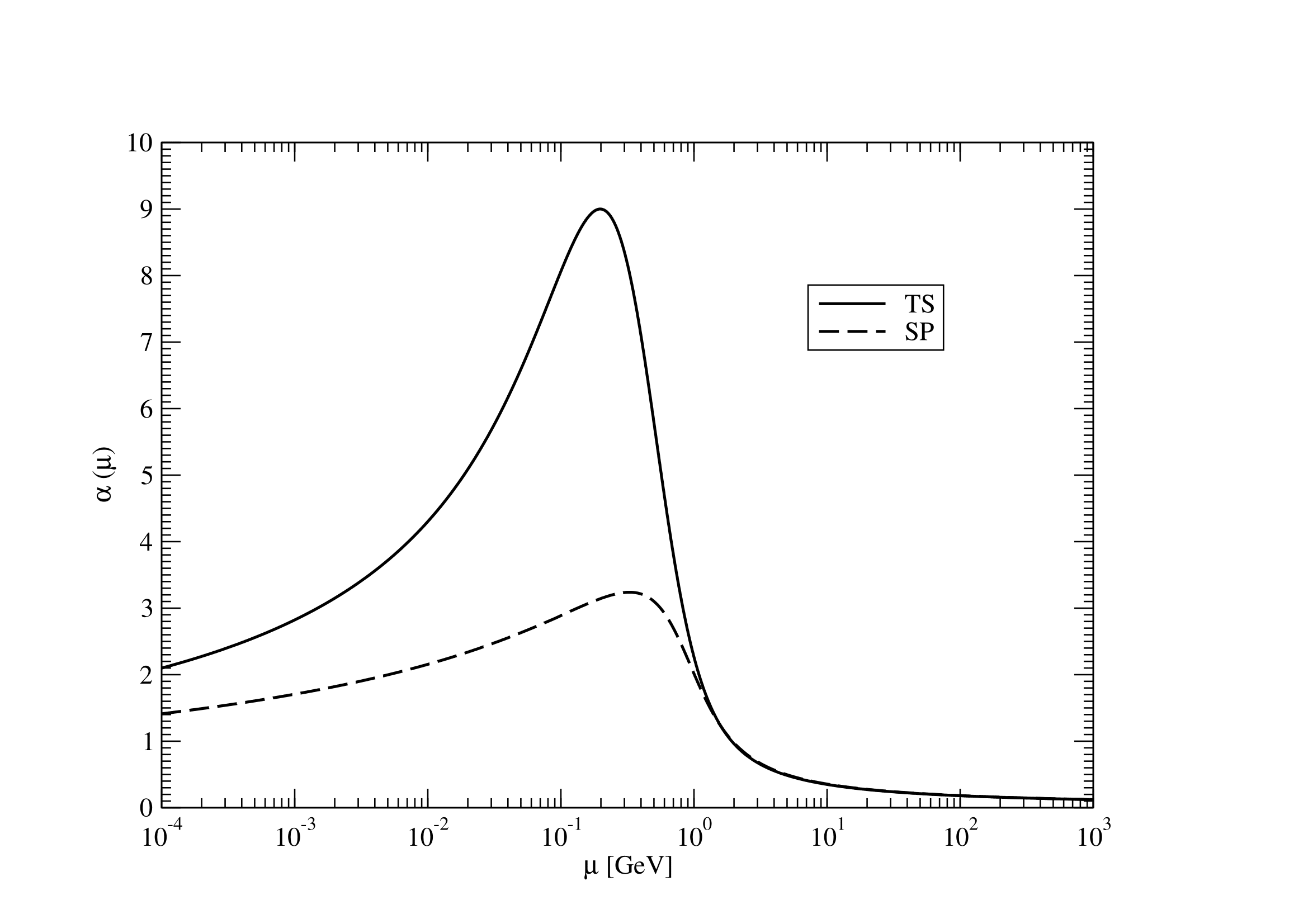
Figure 1: The renormalized strong fine structure constant $\alpha(\mu^{2})=g^{2}(\mu^{2})/4\pi$ as a function of the renormalization scale $\mu$ for the two renormalization schemes which define the coupling constant from the ghost-gluon vertex in the Taylor limit (TS) or at the symmetry point (SP). In both cases, the two-point functions are normalized according to conditions (7)–(9).

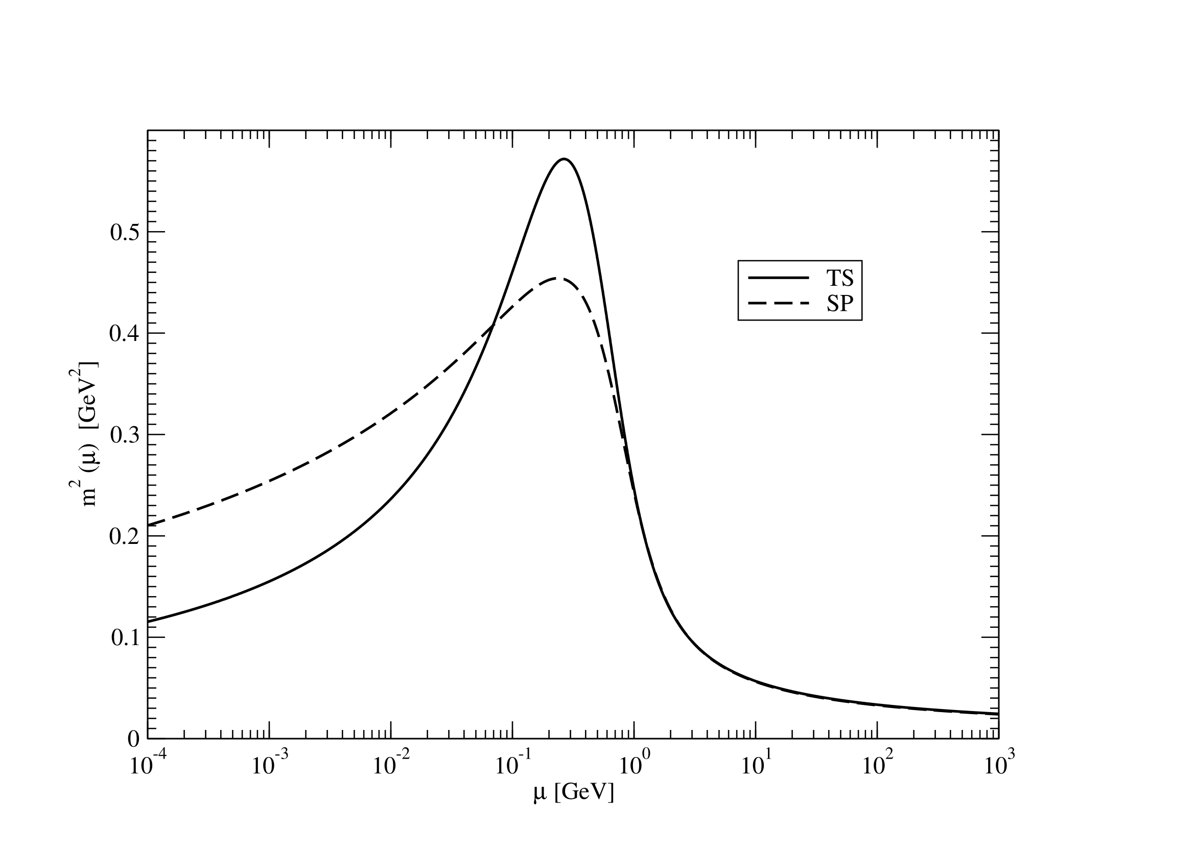
Figure 2: The square of the mass parameter as a function of the renormalization scale $\mu$ for the same renormalization schemes as in Fig. 1.

The behavior of the running mass parameter $m^{2}(\mu^{2})$ is quite similar to the coupling constant, with a logarithmic fall-off towards large $\mu^{2}$, which is consistent with the recovery of the usual, not extended, BRST symmetry in this limit. Rather unexpectedly, the mass parameter also vanishes in the IR limit $\mu^{2}\to 0$. The behavior of $m^{2}(\mu^{2})$ in both limits is governed by the corresponding limits of the beta function $\beta_{m^{2}}$, Eqs. (31) and (33). As remarked before, despite the vanishing of the mass parameter in the IR limit, both the transverse and longitudinal parts of the proper gluonic two-point function tend towards a finite value in this limit, see also below.

Even though the qualitative behavior is the same in both renormalization schemes, in a quantitative sense the renormalization scheme dependence is rather strong. There is a considerable quantitative difference in the maximum values attained by $\alpha(\mu^{2})$ and $m^{2}(\mu^{2})$, particularly in the case of $\alpha(\mu^{2})$, and also in the fall-off of $m^{2}(\mu^{2})$ towards smaller values of $\mu^{2}$. In Figs. 1 and 2, we have integrated the renormalization group equations for $g(\mu^{2})$ and $m^{2}(\mu^{2})$ in SU(2) Yang-Mills theory in the Tissier-Wschebor scheme with the initial values $g(\mu_{0}^{2})=2{.}92$ and $m(\mu_{0}^{2})=0{.}31$ GeV at $\mu_{0}=3$ GeV that we also use later for the fits to the lattice data in this renormalization scheme. In the symmetry point scheme, we use the same value $0{.}31$ GeV for $m(\mu_{0}^{2})$, but determine the value of $g(\mu_{0}^{2})$ at $\mu_{0}=3$ GeV from a perturbative one-loop evaluation of the ghost-gluon vertex at the symmetry point, with the same bare coupling constant as in the Tissier-Wschebor scheme, compare Eqs. (27) and (51). Note that taking the same value for $g(\mu_{0}^{2})$ as in the Tissier-Wschebor scheme would lead to slightly different results for $g(\mu^{2})$ and $m^{2}(\mu^{2})$. For the comparison to the lattice data below we have used the initial values that lead to the best fit to the data for each individual renormalization scheme. In particular, this procedure leads to other values for $g(\mu_{0}^{2})$ and $m(\mu_{0}^{2})$ in the symmetry point scheme than the ones used in Figs. 1 and 2, and the difference between the fits to the gluon and ghost propagators in the two renormalization schemes is much less than one would expect from the comparison of the schemes in Figs. 1 and 2 (see below).

In all derivative schemes (including the simple scheme with $\zeta=1$ and the scale-dependent scheme), the dependence of $\alpha$ and $m^{2}$ on the renormalization scale is qualitatively the same as in Figs. 1 and 2, with the exception of the critical $\zeta=1/3$ scheme. In Figs. 3 and 4, we show the plots of $\alpha(\mu^{2})$ and $m^{2}(\mu^{2})$ in the critical derivative scheme, with the initial values $g=2{.}53$ and $m=0{.}315$ GeV at $\mu=3$ GeV. While the UV behavior is the same as in all the other cases, in the IR limit $\mu^{2}\to 0$ both $\alpha$ and $m^{2}$ tend towards finite (non-zero) values. The actual limiting values are found to depend on the initial values $g(\mu_{0}^{2})$ and $m^{2}(\mu_{0}^{2})$ for the integration of the differential equations. In this sense we find a line of fixed points of the system in the IR limit rather than a single fixed point in this particular renormalization scheme.

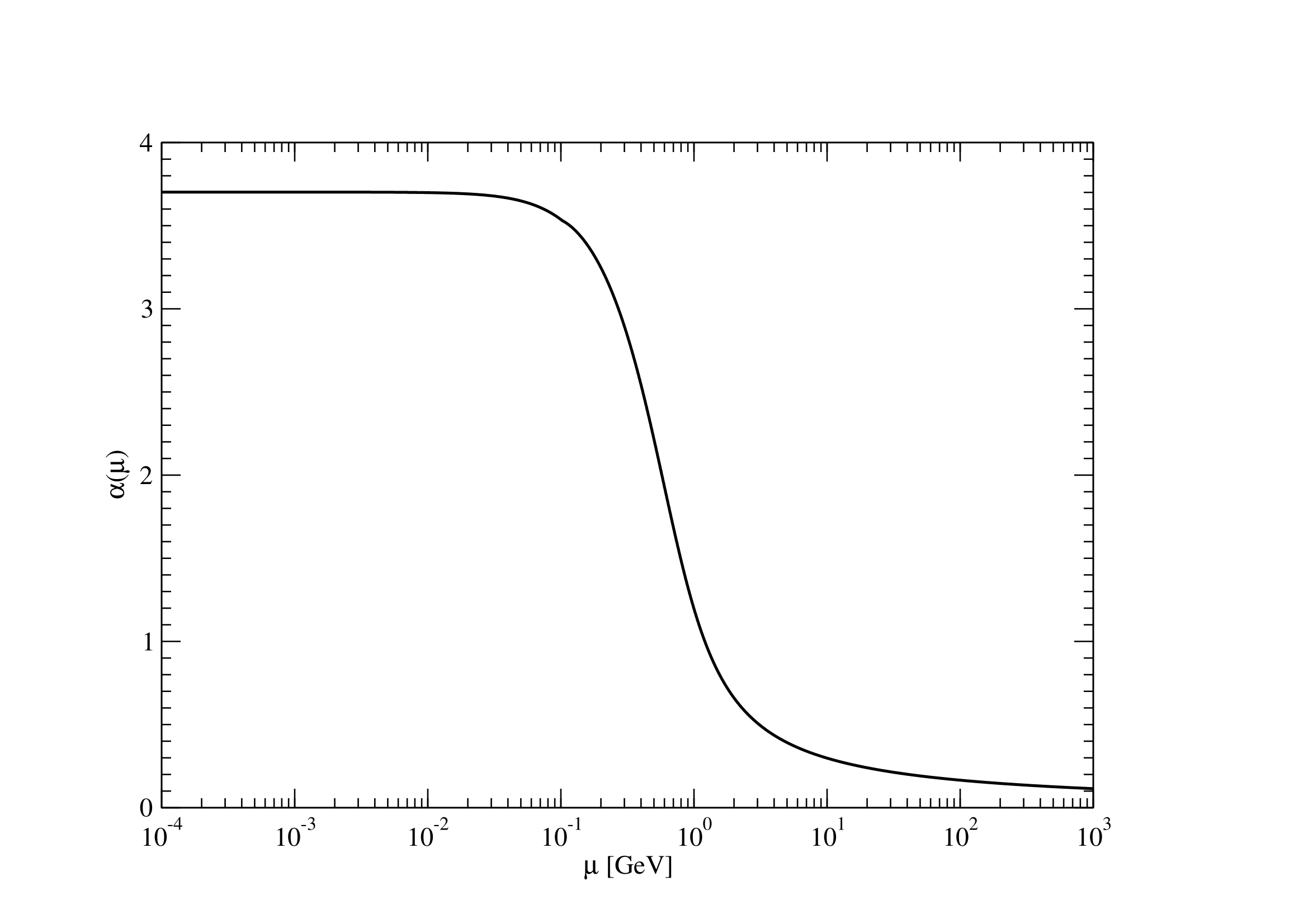
Figure 3: The strong fine structure constant $\alpha$ as a function of the renormalization scale $\mu$ in the critical derivative scheme ($\zeta=1/3$).

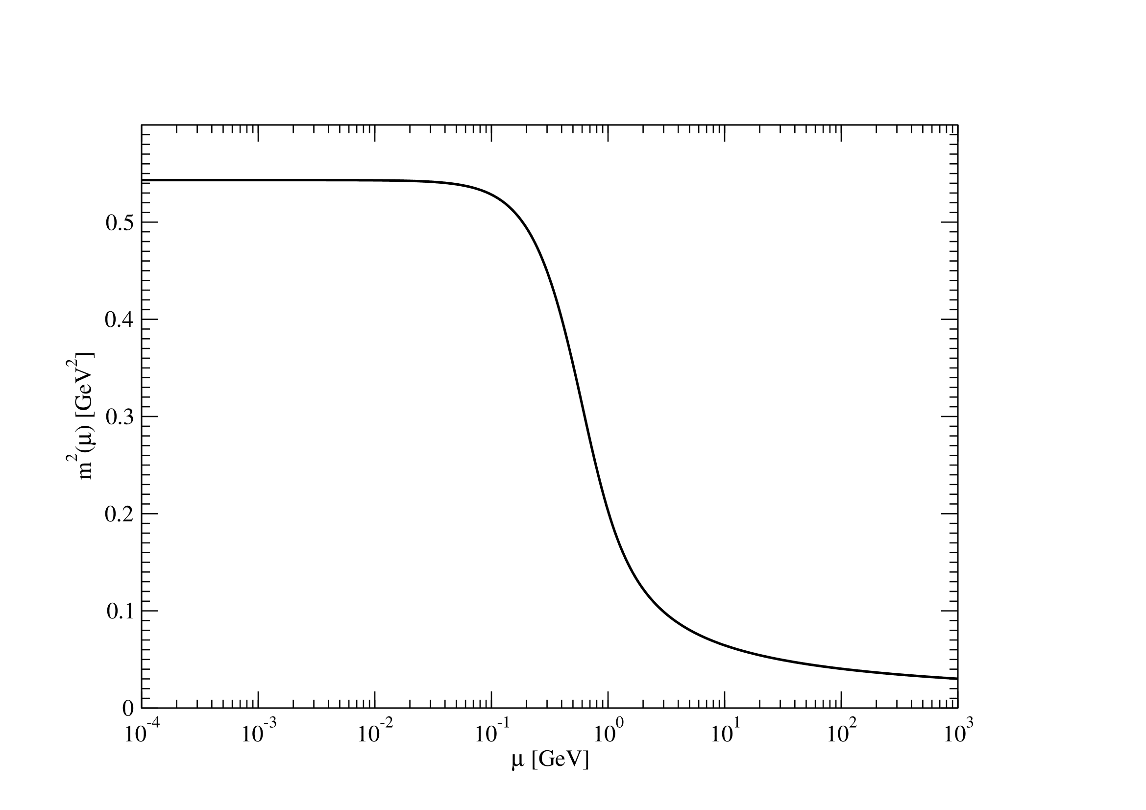
Figure 4: The square of the mass parameter as a function of the renormalization scale $\mu$ in the critical derivative scheme.

We will now present the comparison of our results to the lattice data for the gluon and ghost propagators in SU(2) Yang-Mills theory in the Landau gauge. We shall use the data of Cucchieri and Mendes in Refs. CM08a and CM08b for the comparison. The gauge is fixed on the lattice by minimizing the lattice discretization of the functional

$$\int d^{4}x\,A_{\mu}^{a}(x)A_{\mu}^{a}(x)$$ (75)

along the gauge orbits, which is equivalent to imposing the Landau (Lorenz) gauge condition and restricting the gauge fields to the Gribov region at the same time [if one accepts any local minimum of the functional (75); determining the global minimum of (75) instead would correspond to the restriction of the gauge fields to the fundamental modular region, see also our brief comment footn3 ].

To compare our results with the lattice data, we will determine the initial values $g(\mu_{0}^{2})$ and $m^{2}(\mu_{0}^{2})$ for each renormalization scheme (we shall be using $\mu_{0}=3$ GeV throughout) in such a way that the integration of the Callan-Symanzik equations leads to gluon and ghost propagators that reproduce the results of the lattice simulations for these propagators as closely as possible. We have determined the optimal initial values “by hand”, by varying $g(\mu_{0}^{2})$ and $m^{2}(\mu_{0}^{2})$ in small steps and comparing the plots of the propagators obtained by integrating the Callan-Symanzik equations to the corresponding plots of the lattice data.

The procedure is not as straightforward as it may sound. One of the difficulties is that the lattice propagators are not normalized and hence, for the comparison to the results of the integration of the renormalization group equations, may still be multiplied with arbitrary overall constants (in this sense, there are four parameters to be adjusted). Another difficulty is the comparatively lower precision of the lattice data in the UV regime, cf. the plots of the dressing functions below, where the data begin to oscillate for momenta above approximately $0{.}7$ GeV (for the ghost dressing function), and the results at a given momentum $p=(p^{2})^{1/2}$ depend on the angles the momentum forms with the lattice axes (breaking of continuous rotational invariance on the lattice; the different values are still almost compatible within the statistical errors). For the representation of the lattice data in the figures we identify $p^{2}$ with the improved lattice momentum squared Ma00 .

After experimenting with different possible strategies for quite some time, we have settled on the following procedure for the fits: for any given renormalization scheme, we have determined $g(\mu_{0}^{2})$ and $m^{2}(\mu_{0}^{2})$ (and the multiplicative factor for the normalization of the ghost propagator) in such a way that the best possible fits to the ghost propagator $G_{c}(p^{2})=(\Gamma_{c\bar{c}}(p^{2}))^{-1}$ [see Eq. (6)] and the ghost dressing function $F_{c}(p^{2})=p^{2}\,G_{c}(p^{2})$ are obtained, guided by the eye and making sure that the renormalization group improved results fall inside the statistical error bars of the data for all momenta below $3{.}7$ GeV (for some direction of the momentum with respect to the lattice axes, for the values of $p$ where the breaking of rotational invariance is visible in the lattice data). The latter condition turned out to be impossible to fulfill in the symmetry point scheme, see below. In any case, this procedure fixes $g(\mu_{0}^{2})$ and $m^{2}(\mu_{0}^{2})$ to a fair precision. We remark that a similar strategy, but adjusting our results to the gluon propagator and the gluon dressing function as determined on the lattice rather than using the ghost propagator and the ghost dressing function, or employing the ghost and gluon dressing functions instead, would leave more freedom in the determination of the initial values.

Having thus fixed $g(\mu_{0}^{2})$ and $m^{2}(\mu_{0}^{2})$ for a given renormalization scheme by a fit to the ghost propagator and the ghost dressing function, we use these same initial values to calculate the renormalization group improved gluon propagator $G_{A}(p^{2})=(\Gamma_{AA}^{\perp}(p^{2}))^{-1}$ [see Eq. (6)] and the gluon dressing function $F_{A}(p^{2})=p^{2}\,G_{A}(p^{2})$ (which is the dressing function relative to a massless tree-level propagator). A comparison to the lattice data for the latter functions, after adjusting the respective overall multiplicative factor, gives an indication of how well the renormalization group improvement reproduces the lattice data, for the renormalization scheme considered. We shall show the comparisons for both the gluon propagator and the gluon dressing function in the figures below, since the plots of the propagator give a clearer picture of the quality of the fits in the extreme IR regime, while the plots of the dressing function emphasize the intermediate and large momentum regimes.

Our results are presented in Figs. 5–18 for the different renormalization schemes. In particular, Figs. 5–7 show the best fits for Tissier-Wschebor’s original renormalization scheme, while Figs. 8–10 correspond to the renormalization scheme with the same normalization conditions (7)–(9) for the two-point functions but the renormalized coupling constant defined from the ghost-gluon vertex at the symmetry point as in Eq. (51), rather than in the Taylor limit. While the fit to the ghost dressing function (and also to the ghost propagator) is perfect for momenta up to $3{.}7$ GeV in the Tissier-Wschebor scheme, there are no initial values $g(\mu_{0}^{2})$ and $m^{2}(\mu_{0}^{2})$ for which the renormalization group improved ghost dressing function in the symmetry point scheme would stay within the error bars of the lattice data for momenta below $3{.}7$ GeV. The latter fact demonstrates that it is by no means obvious that a perfect fit to the ghost propagator and the ghost dressing function can be achieved (in this momentum range) by tuning the two initial values and the overall multiplicative constant. The fit to the gluon propagator and the gluon dressing function is also poorer in the symmetry point scheme than in the Tissier-Wschebor (Taylor) scheme. We conclude that the original Tissier-Wschebor scheme leads to better results for the gluon and ghost propagators than the symmetry point scheme.

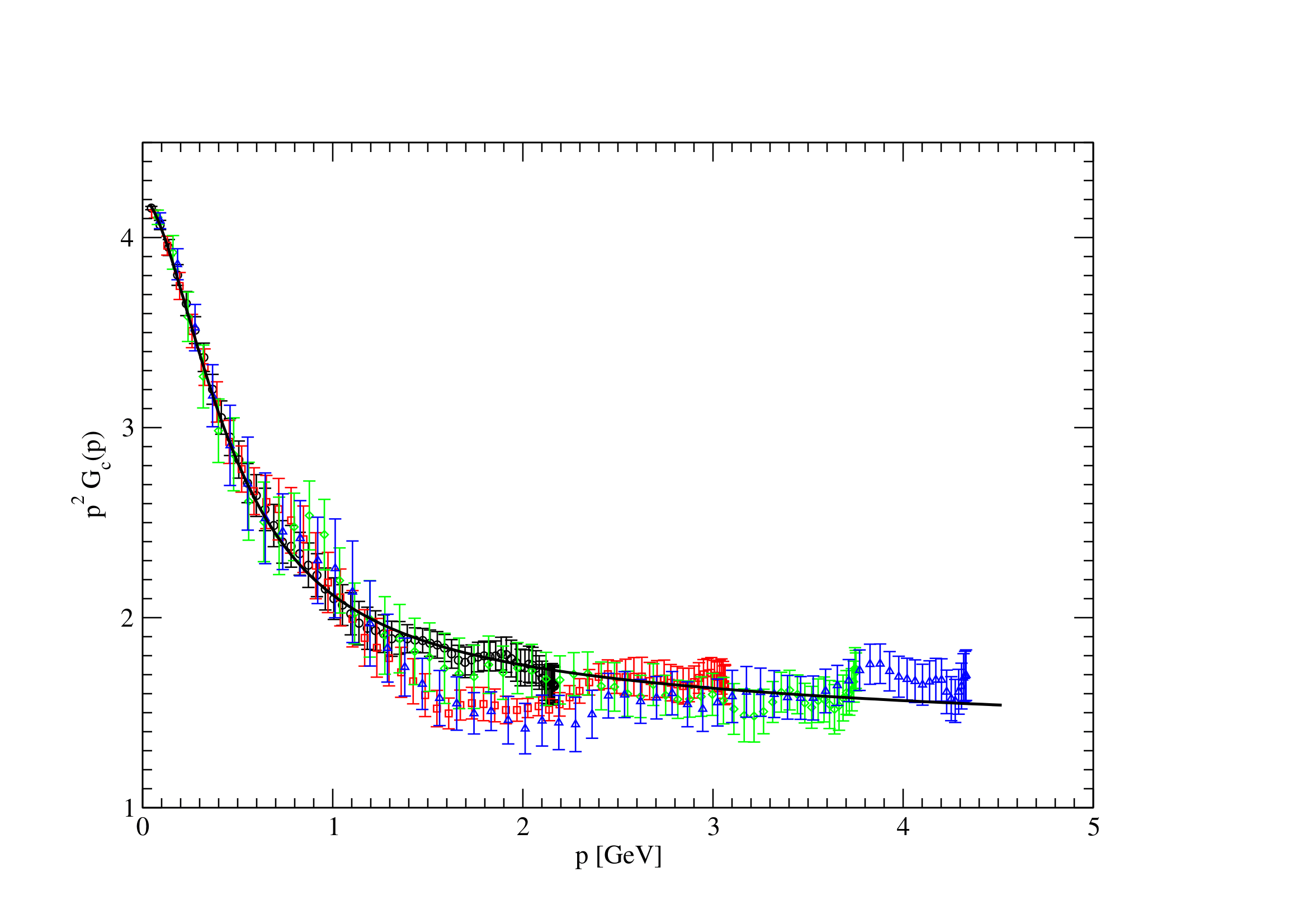
Figure 5: The ghost dressing function $F_{c}(p^{2})=p^{2}\,G_{c}(p^{2})=p^{2}/\Gamma_{c\bar{c}}(p^{2})$ as a function of the momentum $p=(p^{2})^{1/2}$ in the original Tissier-Wschebor scheme defined by the normalization conditions (7)–(9) and the renormalized coupling constant determined from the Taylor limit of the ghost-gluon vertex. The initial conditions for the integration of the renormalization group equations have been chosen in such a way that they produce the best possible fit to the lattice data of Ref. CM08b , which are also represented in the figure. Different colors of the data points (and error bars) in the online version correspond to different directions on the lattice.

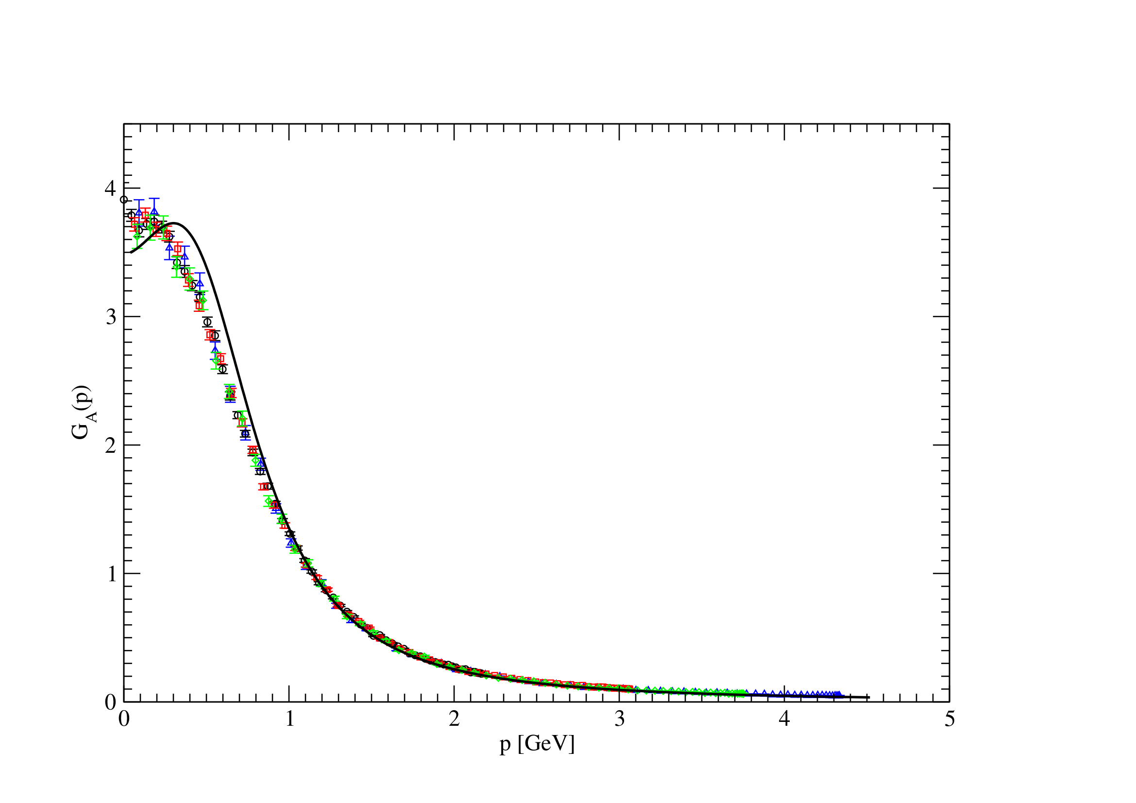
Figure 6: The gluon propagator $G_{A}(p^{2})=1/\Gamma_{AA}^{\perp}(p^{2})$ as a function of momentum in the original Tissier-Wschebor scheme with the same initial conditions for the integration of the renormalization group equations as in Fig. 5, compared to the lattice data of Ref. CM08a .

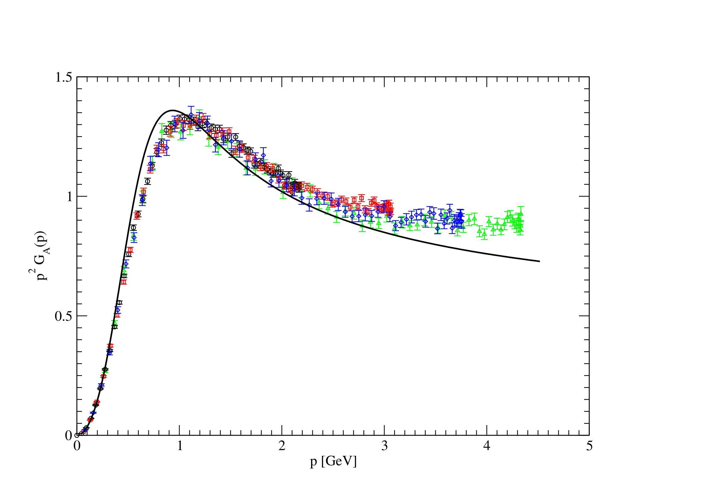
Figure 7: The gluon dressing function $F_{A}(p^{2})=p^{2}\,G_{A}(p^{2})=p^{2}/\Gamma_{AA}^{\perp}(p^{2})$ as a function of momentum in the original Tissier-Wschebor scheme with the same initial conditions as in Fig. 5, compared to the lattice data of Ref. CM08a .

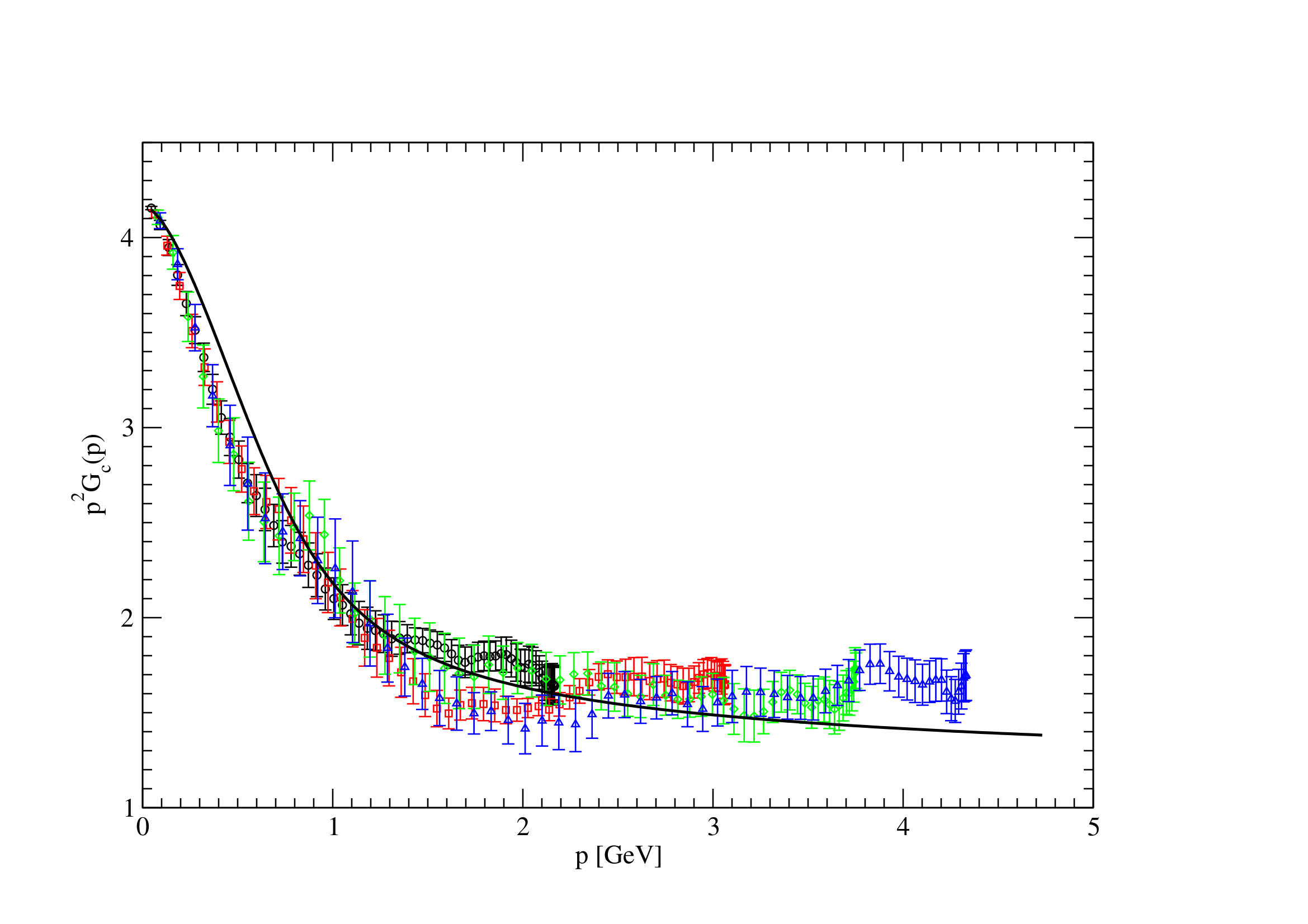
Figure 8: The ghost dressing function $F_{c}(p^{2})=p^{2}\,G_{c}(p^{2})$ as a function of momentum in the renormalization scheme defined through the conditions (7)–(9), but with the renormalized coupling constant determined from the ghost-gluon vertex at the symmetry point. The initial conditions for the integration of the renormalization group equations have been adjusted to produce the best possible fit to the lattice data of Ref. CM08b , which are also represented in the figure.

Figure 9: The gluon propagator $G_{A}(p^{2})$ as a function of momentum in the symmetry point scheme [with normalization conditions (7)–(9)] with the same initial conditions for the integration of the renormalization group equations as in Fig. 8, compared to the lattice data from Ref. CM08a .

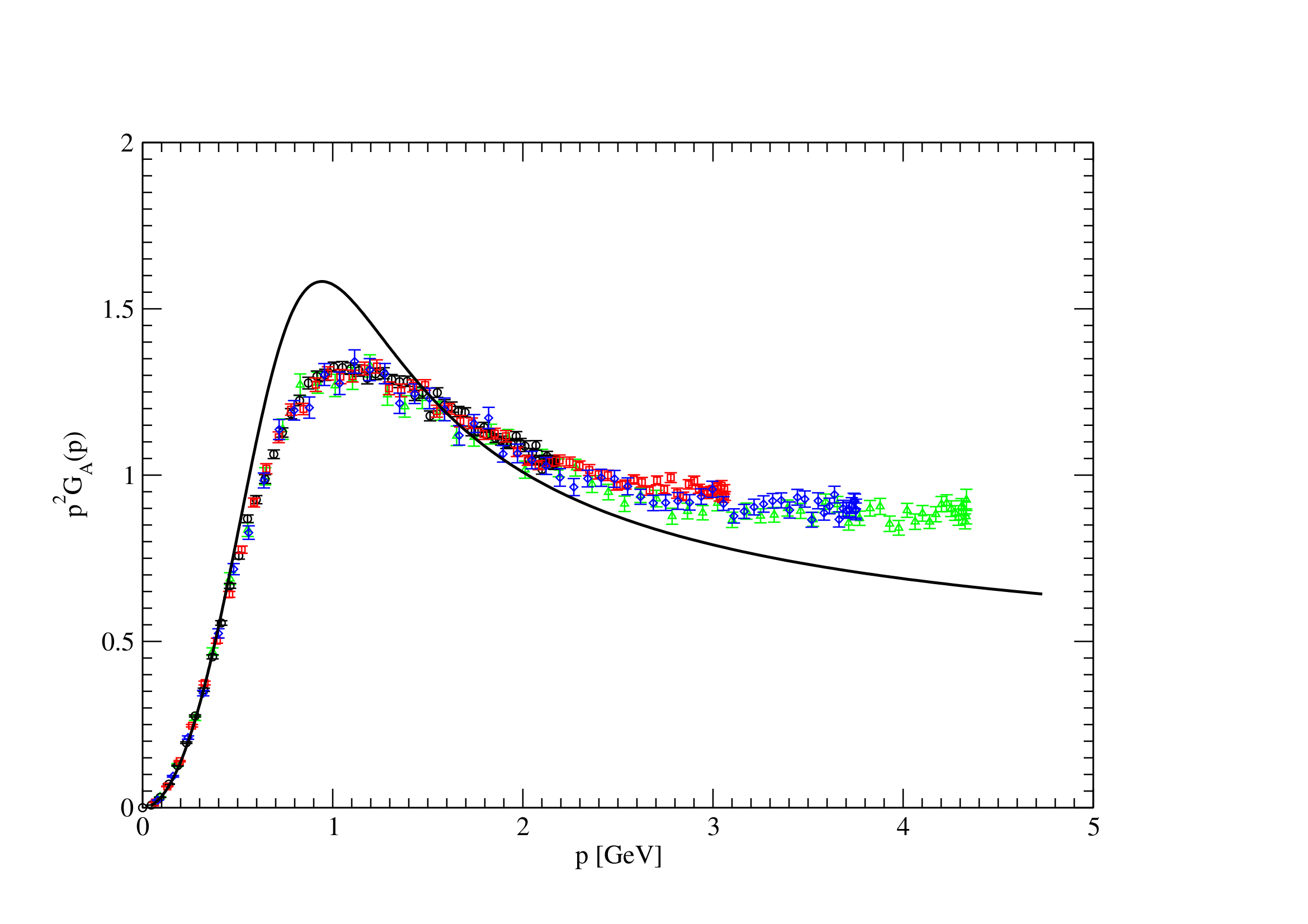
Figure 10: The gluon dressing function $F_{A}(p^{2})=p^{2}\,G_{A}(p^{2})$ as a function of momentum in the symmetry point scheme with the same initial conditions as in Fig. 8, compared to the lattice data of Ref. CM08a .

Note that our fits to the lattice data differ somewhat from the ones obtained by Peláez, Tissier and Wschebor in Ref. TW13 , in particular for the ghost dressing function, even though the differential equations we have used are exactly the same. The reason for this difference appears to be that Peláez, Tissier and Wschebor have fitted the renormalization group improved results for the ghost dressing function to the lattice data for momenta in the directions $(0,0,1,1)$ and $(1,1,1,1)$ on the lattice (red and blue data points in the online version), while we have found better overall fits by adjusting our curves to the data for momentum directions $(0,0,0,1)$ and $(0,1,1,1)$, in the momentum regime where the breaking of rotational invariance on the lattice is visible.

We present the results for all other renormalization schemes, with the corresponding normalization conditions described in Subsection II.2, in Figs. 11–18. All these plots are for the case where the renormalized coupling constant is defined from an evaluation of the ghost-gluon vertex in the Taylor limit, Eq. (27), with the exception of the scale-dependent derivative scheme where we have also considered the scale-dependent definition (56) of the coupling constant. Just as in the case of the normalization conditions (7)–(9) before, the definition of the coupling constant from the ghost-gluon vertex at the symmetry point leads to less satisfactory fits to the lattice data for the ghost and gluon propagators (and dressing functions) than the definition of the coupling constant that uses the Taylor limit of the same vertex, with the same normalization conditions for the two-point functions. In the paragraph that contains Eq. (56), we had already presented an intuitive argument in favor of the Taylor limit for the description of the IR regime.

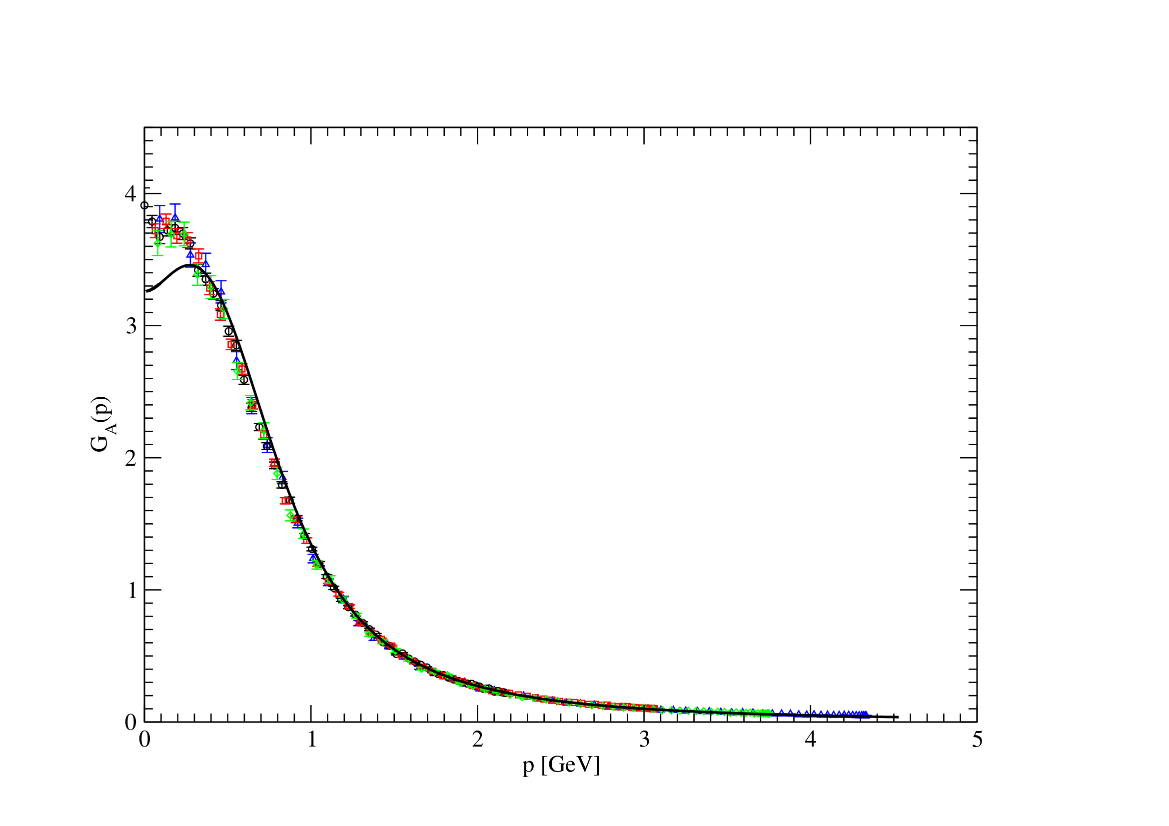
Figure 11: The gluon propagator $G_{A}(p^{2})$ as a function of momentum in the simple derivative scheme ($\zeta=1$), where the renormalized coupling constant is defined from the ghost-gluon vertex in the Taylor limit. The initial conditions for the integration of the renormalization group equations are chosen in such a way that they produce the best possible fit to the ghost propagator and the ghost dressing function obtained in the lattice simulations of Ref. CM08b . The lattice data of Ref. CM08a for the gluon propagator are also shown in the figure for comparison.

Figure 12: The gluon dressing function $F_{A}(p^{2})=p^{2}\,G_{A}(p^{2})$ as a function of momentum in the simple ($\zeta=1$) derivative scheme with the same initial conditions as in Fig. 11, compared to the lattice data of Ref. CM08a .

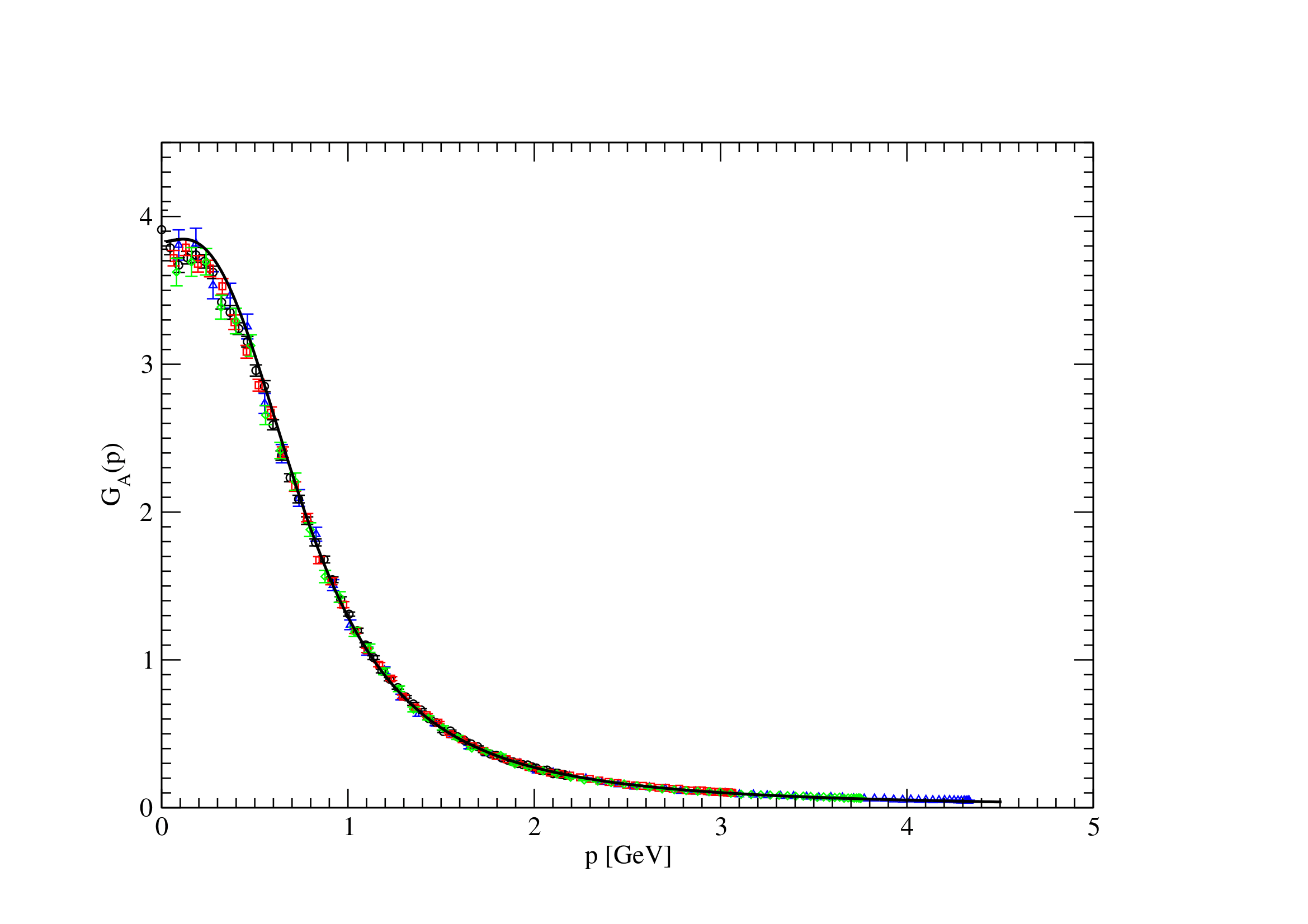
Figure 13: The gluon propagator $G_{A}(p^{2})$ as a function of momentum in the critical derivative scheme ($\zeta=1/3$), where the renormalized coupling constant is defined from the ghost-gluon vertex in the Taylor limit. The initial conditions for the integration of the renormalization group equations are chosen in such a way that they produce the best possible fit to the ghost propagator and the ghost dressing function obtained in the lattice simulations of Ref. CM08b . The lattice data of Ref. CM08a for the gluon propagator are also shown in the figure for comparison.

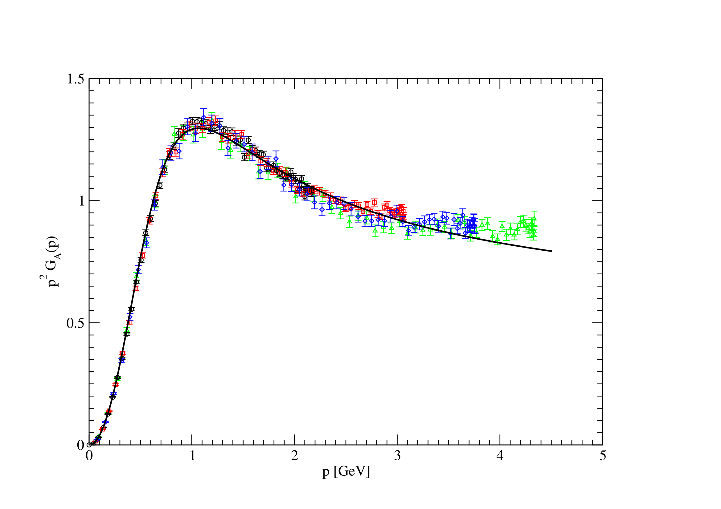
Figure 14: The gluon dressing function $F_{A}(p^{2})=p^{2}\,G_{A}(p^{2})$ as a function of momentum in the critical derivative scheme with the same initial conditions as in Fig. 13, compared to the lattice data of Ref. CM08a .

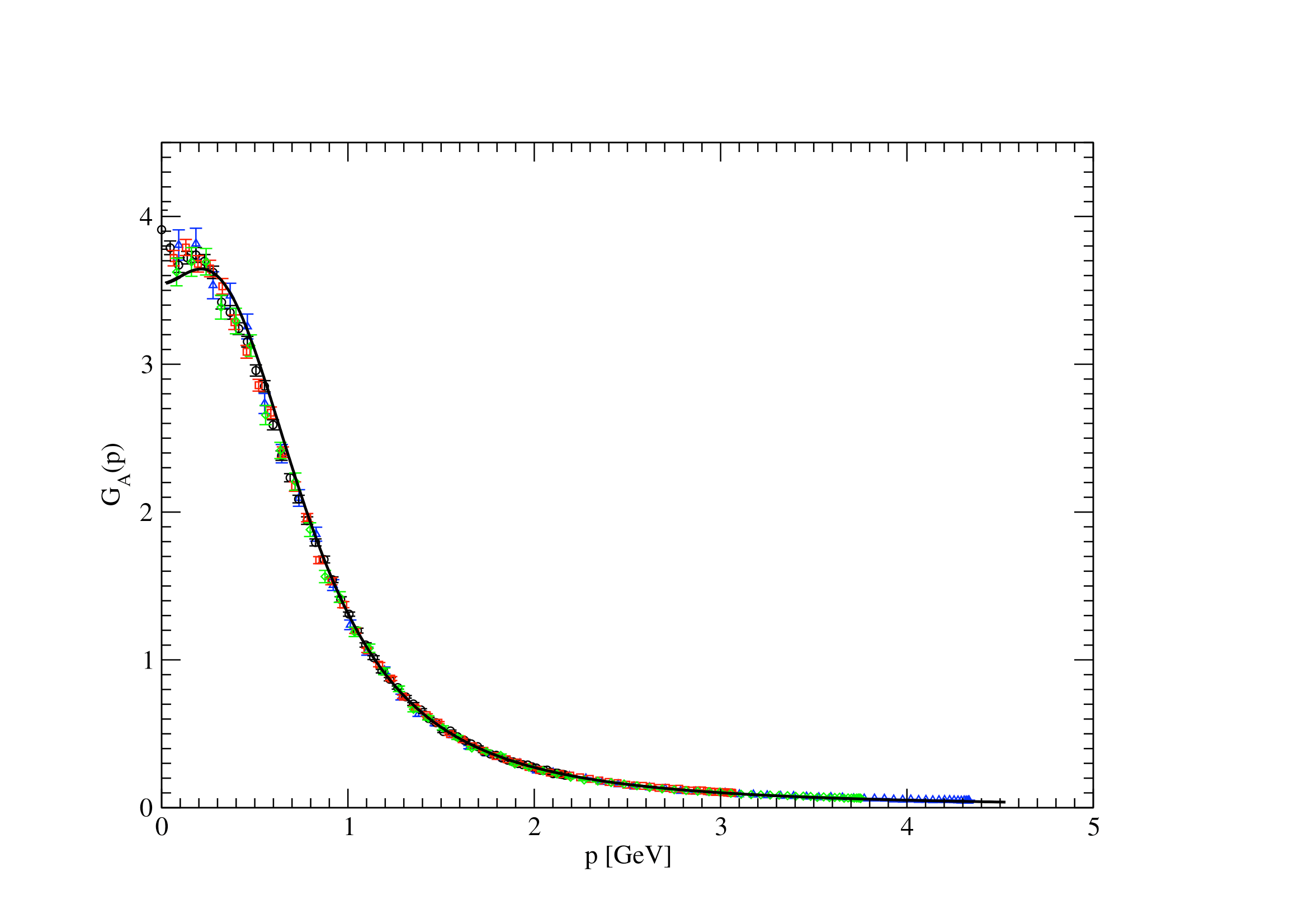
Figure 15: The gluon propagator $G_{A}(p^{2})$ as a function of momentum in the scale-dependent derivative scheme [with $\zeta$ from Eq. (49)], where the renormalized coupling constant is defined from the ghost-gluon vertex in the Taylor limit. The initial conditions for the integration of the renormalization group equations are chosen in such a way that they produce the best possible fit to the ghost propagator and the ghost dressing function obtained in the lattice simulations of Ref. CM08b . The lattice data of Ref. CM08a for the gluon propagator are also shown in the figure for comparison.

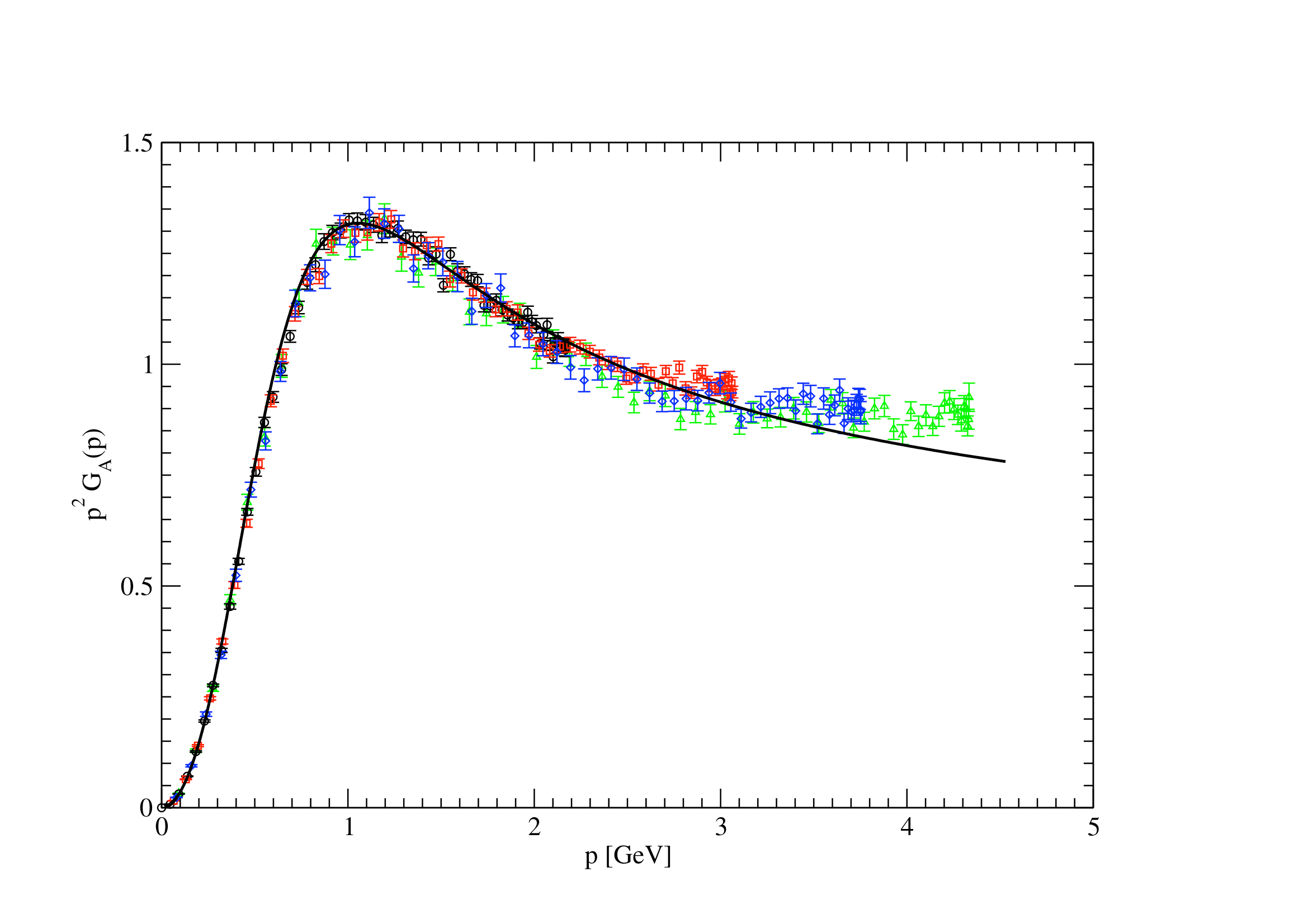
Figure 16: The gluon dressing function $F_{A}(p^{2})=p^{2}\,G_{A}(p^{2})$ as a function of momentum in the scale-dependent derivative scheme with the coupling constant defined from the Taylor limit of the ghost-gluon vertex and using the same initial conditions as in Fig. 15, compared to the lattice data of Ref. CM08a .

Figure 17: The gluon propagator $G_{A}(p^{2})$ as a function of momentum in the scale-dependent derivative scheme with the scale-dependent definition (56) of the renormalized coupling constant. The initial conditions for the integration of the renormalization group equations are chosen in such a way that they produce the best possible fit to the ghost propagator and the ghost dressing function obtained in the lattice simulations of Ref. CM08b . The lattice data of Ref. CM08a for the gluon propagator are also shown in the figure for comparison.

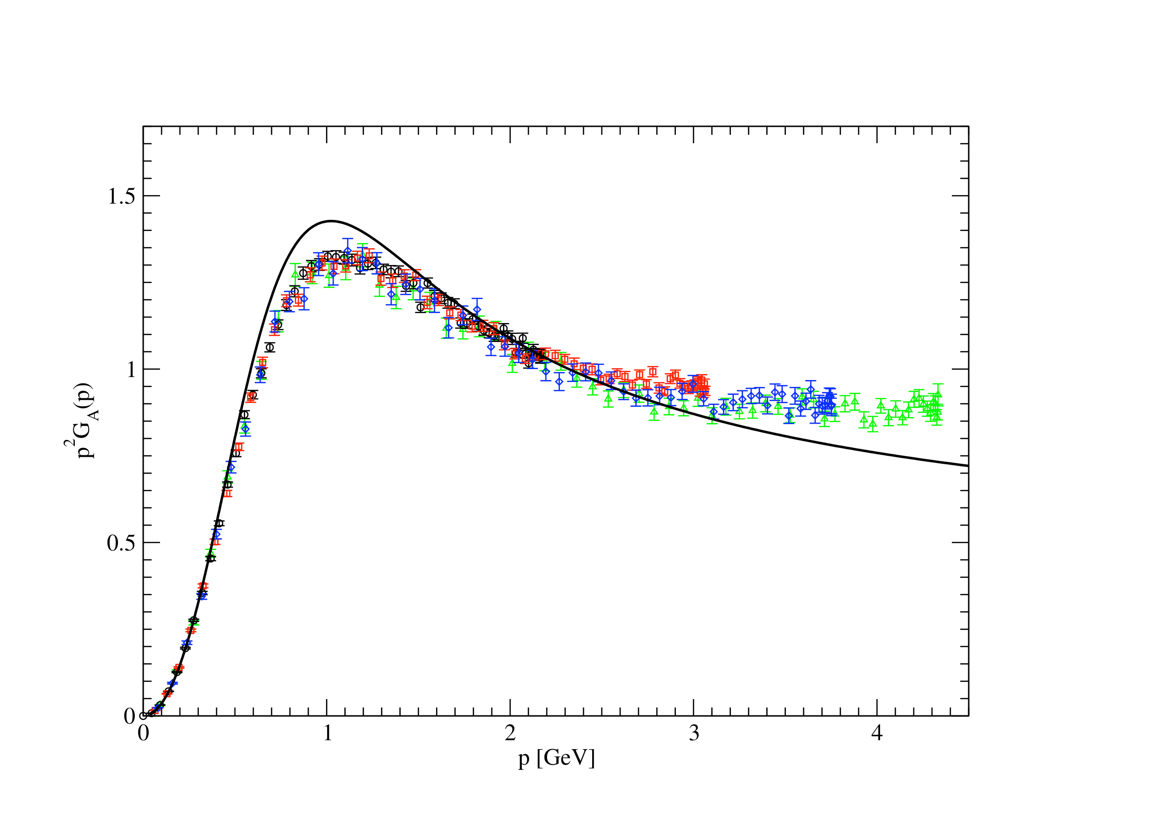
Figure 18: The gluon dressing function $F_{A}(p^{2})=p^{2}\,G_{A}(p^{2})$ as a function of momentum in the scale-dependent derivative scheme with the scale-dependent definition of the renormalized coupling constant and using the same initial conditions as in Fig. 17, compared to the lattice data of Ref. CM08a .

We do not show the fits to the ghost dressing functions in Figs. 11–18 since they are very similar to Fig. 5 for the Tissier-Wschebor scheme in all cases (that use the Taylor scheme for the coupling constant), i.e., they are perfect fits for momenta below $3{.}7$ GeV, and the same is true for the fits to the ghost propagator function. In general, our results compare fairly well to the lattice simulations, in particular when one considers that we have calculated the flow functions only to one-loop order. There is inevitably an element of subjectivity left in our fitting procedure, but from the figures we have produced it appears that, among all the renormalization schemes that we have considered, the best fits to the lattice data can be achieved in the critical ($\zeta=1/3$) and the scale-dependent derivative schemes (with the renormalized coupling constant defined from the ghost-gluon vertex in the Taylor limit). In particular, these derivative schemes reproduce the gluon and ghost propagators obtained in the lattice simulations more closely than Tissier-Wschebor’s original renormalization scheme.

In all renormalization schemes we have found a decrease of the gluon propagator $G_{A}(p^{2})$ towards smaller momenta in the extreme IR regime. This decrease is not (clearly) seen in the lattice data, although at least a slight decrease cannot be excluded from the present data, either. We shall analytically confirm in the following subsection, through an expansion for small momenta, that the decrease is present in all renormalization schemes described in the previous section, in particular for all values $\zeta\geq 1/3$ in the derivative schemes, and it can thus be considered a general feature of the gluon propagator in the renormalization group improved perturbative approach to Yang-Mills theory. In principle, the effect could be overturned by higher-loop contributions to the flow functions. However, this seems unlikely given that the decrease is already visible in the plain perturbative one-loop expression (15) for $\Gamma^{\perp}_{AA}(p^{2})$, where the term proportional to $(p^{2}\ln(p^{2}/m^{2}))$ dominates the $p^{2}$-dependence in the limit $p^{2}\to 0$.

The decrease of the gluon propagator function towards small momenta implies a non-monotonous momentum dependence of the propagator that is clearly incompatible with the existence of a spectral representation with a non-negative spectral function $\rho(M^{2})$,

$$G_{A}(p^{2})=\int_{0}^{\infty}\frac{dM^{2}}{2\pi}\,\frac{\rho(M^{2})}{p^{2}+M^{2}}\,,$$ (76)

as recognized before in Refs. CFM16 and RSTW17 . In other words, the non-monotony of the gluon propagator is sufficient for the violation of positivity.

From a comparison of the extreme IR behavior of the numerical solutions in the derivative schemes for different values of the parameter $\zeta$, one concludes that the decrease of the gluon propagator towards smaller momenta gets more pronounced for larger values of $\zeta$ (compare Figs. 11 and 13 for $\zeta=1$ and $\zeta=1/3$, respectively; this tendency can be seen to extend to larger values of $\zeta$). This $\zeta$-dependence of the IR decrease is at least one of the reasons why, among the scale-independent derivative schemes, the scheme with the smallest possible (critical) value $\zeta=1/3$ gives the best fit to the lattice data.

Even in the critical and the scale-dependent derivative schemes, the renormalization group improved curves for the gluon dressing function in Figs. 14 and 16 seem to systematically deviate from the lattice data for momenta above (roughly) $3{.}5$ GeV. The same deviation of the gluon dressing function from the lattice data in the UV regime is seen in all the other renormalization schemes as well, typically already at slightly lower momentum scales. Our interpretation is that in this case it is the lattice data that do not reproduce the correct UV behavior with sufficient precision. In fact, the value of the lattice spacing used in the numerical calculations of Ref. CM08a is $a=1{.}066$ $\mbox{GeV}^{-1}$ in physical units, so that momenta around $3{.}5$ GeV are already of the order of the lattice cutoff $(\pi/a)$ and the corresponding results cannot be compared to calculations in the continuum (remember that the values that we cite for the momenta correspond to improved lattice momenta Ma00 ).

We can, however, compare the UV behavior of our renormalization group improved results to the lattice simulations on finer (but smaller) lattices in Ref. BCL04 , where the physical scale was fixed via the string tension in exactly the same way as in Ref. CM08a . In Ref. BCL04 , the results of lattice calculations of the gluon and ghost dressing functions in the UV regime were compared to the usual (renormalization group improved) perturbative two-loop propagators. It was found that the perturbative propagators with a value of $1{.}2(1)$ GeV for $\Lambda_{\text{QCD}}$, together with very small coefficients of the renormalization scheme dependent two-loop terms (as in the $\overline{\text{MS}}$ scheme), correctly reproduced the lattice results for the dressing functions in the UV. Due to the strong renormalization scheme dependence of $\Lambda_{\text{QCD}}$, we cannot relate the latter result for $\Lambda_{\text{QCD}}$ [via Eq. (80)] directly to the values we have used for $g(\mu_{0})$ at $\mu_{0}=3$ GeV in our fits, but we can compare the perturbative two-loop dressing functions to our numerical results for these dressing functions in the UV. We obtain a value for $\Lambda_{\text{QCD}}$ of around $1{.}0$ GeV for the fit of the perturbative two-loop propagators to the numerical curves obtained from the renormalization group improvement in the scale-dependent derivative scheme, and a value of about $0{.}95$ GeV for the critical derivative scheme, where we have set the coefficients of the renormalization scheme dependent two-loop terms to zero. These values are quite remarkably close to and, within the error bars, consistent with $\Lambda_{\text{QCD}}=1{.}2$ GeV found from the comparison of the perturbative two-loop propagators with the lattice data of Ref. BCL04 . In contrast, if one tries to fit the perturbative two-loop results to the lattice data of Refs. CM08a ; CM08b in the UV, one finds a value of approximately $0{.}56$ GeV for $\Lambda_{\text{QCD}}$.

The last issue we shall discuss in this subsection is the violation of the Slavnov-Taylor identity (60) in all derivative schemes, including the simple ($\zeta=1$) scheme. As we have previously explained in detail, Eq. (60) is a consequence of the massive extension (2) of the BRST symmetry and predicts the combination $(\Gamma_{c\bar{c}}(p^{2})\Gamma_{AA}^{\parallel}(p^{2})/p^{2})$ to be $p^{2}$-independent to all orders of perturbation theory, even if the renormalization scheme should not properly preserve the extended BRST symmetry. We have already mentioned in the previous subsection that the renormalization group improvement in such a renormalization scheme (with the flow functions determined to a given finite loop order) could lead to a $p^{2}$-dependence of the combination $(\Gamma_{c\bar{c}}(p^{2})\Gamma_{AA}^{\parallel}(p^{2})/p^{2})$, thus contradicting Eq. (60).

In Fig. 19 we have plotted this combination, normalized by dividing through the value of $m^{2}$ at the renormalization scale $\mu=3$ GeV, against $p=(p^{2})^{1/2}$ for the simple ($\zeta=1$) derivative scheme, the critical ($\zeta=1/3$) and the scale-dependent derivative schemes, using our numerical results for the proper two-point functions in each of these renormalization schemes. One clearly sees a nontrivial $p^{2}$-dependence in all these schemes. We shall confirm this finding, furthermore, in the next subsection with the help of an analytical calculation. To compare with, in Tissier-Wschebor’s original renormalization scheme we find the same normalized combination, both numerically and analytically, to give a $p^{2}$-independent constant, which is also represented in Fig. 19. Incidentally, at the renormalization scale $p=\mu=3$ GeV, the normalized combination $(\Gamma_{c\bar{c}}(p^{2})\Gamma_{AA}^{\parallel}(p^{2})/p^{2}m^{2}(\mu^{2}))$ reduces to $\Gamma_{c\bar{c}}(\mu^{2})/\mu^{2}$ as a consequence of the normalization condition (8) or (42). The different value of the normalized combination at this scale in the original Tissier-Wschebor scheme as opposed to the derivative schemes is due to the different normalization conditions (9) and (37) for the ghost two-point function.

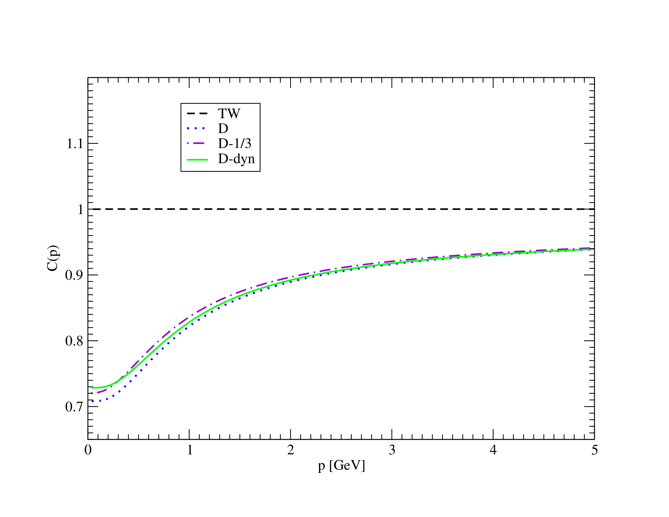
Figure 19: The normalized combination $C(p^{2})=\Gamma_{c\bar{c}}(p^{2})\Gamma_{AA}^{\parallel}(p^{2})/p^{2}m^{2}(\mu^{2})$ as a function of momentum for the renormalization group improved proper two-point functions in the Tissier-Wschebor scheme (TW), the simple derivative scheme with $\zeta=1$ (D), the critical ($\zeta=1/3$) derivative scheme (D-1/3) and the scale-dependent derivative scheme (D-dyn).

One may then argue that the derivative schemes do not constitute proper renormalizations of the theory, inasmuch as they do not respect (in the absence of anomalies) all the symmetries of the “classical” action. As already discussed in the previous section, this is not our point of view here because we do not consider the massive extension of the BRST symmetry to be a fundamental symmetry of the theory, i.e., of a formulation of Yang-Mills theory in the Landau gauge that takes care of the existence of gauge copies in the standard Faddeev-Popov quantization by restricting the integral over the gauge fields to the Gribov region. Rather, we look at the extended BRST symmetry as an “accidental” symmetry of the simplest renormalizable effective theory that gives an accurate description of the crossover from the UV to the IR fixed point of the full theory, at least as far as the momentum dependence of the propagators is concerned, which is the Curci-Ferrari model (1).

III.3 Analytical results

It is reassuring to back up the more interesting findings of the numerical integration of the Callan-Symanzik equations with analytical calculations, for instance to confirm that certain properties hold for all values of the parameter $\zeta$ in the derivative schemes. Furthermore, some of the analytical expressions, although approximate, are of interest by themselves.

We will consider the description of the UV regime first. In the limit of large values of the renormalization scale, $\mu^{2}\gg m^{2}(\mu^{2})$, the one-loop expressions for the flow functions, to leading order in an expansion in powers of $(m^{2}/\mu^{2})$, are the same in all (successful) renormalization schemes considered in the previous section, namely

$$\gamma_{A}=-\frac{13}{6}\frac{Ng^{2}}{(4\pi)^{2}}\,,\quad\gamma_{c}=-\frac{3}{4}\frac{Ng^{2}}{(4\pi)^{2}}$$ (77)

and

$$\beta_{g}=-\frac{11}{6}\frac{Ng^{2}}{(4\pi)^{2}}\,g\,.$$ (78)

These are, of course, the very well-known perturbative expressions in the theory without a gluon mass term. The beta function of the mass,

$$\beta_{m^{2}}=-\frac{35}{12}\frac{Ng^{2}}{(4\pi)^{2}}\,m^{2}\,,$$ (79)

is also the same in all renormalization schemes to leading order in $(m^{2}/\mu^{2})$.

The integration of the differential equation for the renormalized coupling constant to this order leads to the well-known result

$$\frac{Ng^{2}(\mu^{2})}{(4\pi)^{2}}=\left(\frac{11}{3}\,\ln\frac{\mu^{2}}{\Lambda_{\text{UV}}^{2}}\right)^{-1}\,,$$ (80)

where the scale $\Lambda_{\text{UV}}$ is defined through the same relation (80) in terms of the renormalized coupling constant $g(\mu_{0}^{2})$ at some reference scale $\mu_{0}$. The scale $\Lambda_{\text{UV}}$ is the same as the characteristic scale $\Lambda_{\text{QCD}}$ of perturbative Yang-Mills theory (or, generally, of perturbative QCD), but here we prefer the notation $\Lambda_{\text{UV}}$ to distinguish it from an analogous (different) characteristic scale $\Lambda_{\text{IR}}$ that will be introduced below for the description of the infrared regime of the theory.

With the formula (80) for the running coupling constant, one can integrate the differential equation for the renormalized mass parameter, with the “universal” result

$$m^{2}(\mu^{2})=m^{2}(\mu_{0}^{2})\left(\frac{\ln\,(\mu_{0}^{2}/\Lambda_{\text{UV}}^{2})}{\ln\,(\mu^{2}/\Lambda_{\text{UV}}^{2})}\right)^{35/44}$$ (81)

to leading order in $(m^{2}(\mu_{0}^{2})/\mu_{0}^{2})$ and $(m^{2}(\mu^{2})/\mu^{2})$. Equation (66), upon substituting Eq. (81) for $m^{2}(\mu^{2})$, and Eq. (80) for $g^{2}(\mu^{2})$ in the formula (77) for $\gamma_{A}(\mu^{2})$, then leads to the equally universal result for the longitudinal part of the proper gluonic two-point function

$$\Gamma^{\parallel}_{AA}(p^{2},\mu^{2})=m^{2}(\mu^{2})\left(\frac{\ln\,(\mu^{2}/\Lambda_{\text{UV}}^{2})}{\ln\,(p^{2}/\Lambda_{\text{UV}}^{2})}\right)^{9/44}\,,$$ (82)

where we have put $\mu$ equal to the reference scale $\mu_{0}$ [alternatively, we may use Eq. (81) to write $m^{2}(\mu_{0}^{2})$ in terms of $m^{2}(\mu^{2})$]. Thus both the mass parameter and the longitudinal part of the gluonic two-point function tend logarithmically to zero in the UV limit $p^{2}\to\infty$ ($\mu^{2}\to\infty$ in the case of the mass parameter), in particular, the proper two-point function becomes transverse in this limit. Note that the transverse part of the gluonic two-point function increases with $p^{2}$ in the UV and dominates over the longitudinal part by a factor of $p^{2}/m^{2}(\mu^{2})$ [and a power of $\ln(p^{2}/\Lambda_{\text{UV}}^{2})$, see below].

As for the ghost two-point function, using Eq. (80) for $g^{2}(\mu^{2})$ in the formula (77) for $\gamma_{c}(\mu^{2})$ gives

$$\exp\left(-\int_{\mu^{2}}^{p^{2}}\frac{d\mu^{\prime\,2}}{\mu^{\prime\,2}}\,\gamma_{c}(\mu^{\prime\,2})\right)=\left(\frac{\ln\,(p^{2}/\Lambda_{\text{UV}}^{2})}{\ln\,(\mu^{2}/\Lambda_{\text{UV}}^{2})}\right)^{9/44}$$ (83)

in all renormalization schemes. Then Eq. (64) immediately yields

$$\Gamma_{c\bar{c}}(p^{2},\mu^{2})=p^{2}\left(\frac{\ln\,(p^{2}/\Lambda_{\text{UV}}^{2})}{\ln\,(\mu^{2}/\Lambda_{\text{UV}}^{2})}\right)^{9/44}$$ (84)

in Tissier-Wschebor’s original scheme. For all the other (derivative) schemes, we have from Eq. (71) that

$$\Gamma_{c\bar{c}}(p^{2},\mu^{2})=\int_{0}^{p^{2}}dp^{\prime\,2}\left(\frac{\ln\,(p^{\prime\,2}/\Lambda_{\text{UV}}^{2})}{\ln\,(\mu^{2}/\Lambda_{\text{UV}}^{2})}\right)^{9/44}\,.$$ (85)

Note that Eq. (83) is expected to be valid only in the UV regime, but the contribution to the integral over $p^{\prime\,2}$ from this regime is proportional to $p^{2}$ [times some power of $\ln(p^{2}/\Lambda_{\text{UV}}^{2})$, see below] and thus dominates the integral, the contributions from the other momentum regimes being suppressed by a relative factor of $1/p^{2}$.

The integral in Eq. (85) can be expressed in closed form in terms of a confluent hypergeometric or Kummer function of $\ln(p^{2}/\Lambda_{\text{UV}}^{2})$. However, a much more intuitive representation for our purposes is obtained by writing the integral in the form of a power series in $(\ln(p^{2}/\Lambda_{\text{UV}}^{2}))^{-1}$,

$$\int_{0}^{p^{2}}dp^{\prime\,2}\left(\frac{\ln\,(p^{\prime\,2}/\Lambda_{\text{UV}}^{2})}{\ln\,(\mu^{2}/\Lambda_{\text{UV}}^{2})}\right)^{9/44}$$

$$=p^{2}\left(\frac{\ln\,(p^{2}/\Lambda_{\text{UV}}^{2})}{\ln\,(\mu^{2}/\Lambda_{\text{UV}}^{2})}\right)^{9/44}\left[1+\frac{A_{1}}{\ln\,(p^{2}/\Lambda_{\text{UV}}^{2})}+\frac{A_{2}}{\big{(}\ln\,(p^{2}/\Lambda_{\text{UV}}^{2})\big{)}^{2}}+\ldots\right]\,.$$ (86)

A recursion formula for the coefficients $A_{i}$, $i=1,2,\ldots$, can easily be derived by differentiating both sides of this equation with respect to $\ln(p^{2}/\Lambda_{\text{UV}}^{2})$. The result coincides with the use of the known asymptotic expansion of the Kummer function [for large values of $\ln(p^{2}/\Lambda_{\text{UV}}^{2})$]. To first order in $(\ln(p^{2}/\Lambda_{\text{UV}}^{2}))^{-1}$, one obtains

$$\Gamma_{c\bar{c}}(p^{2},\mu^{2})=p^{2}\left(\frac{\ln\,(p^{2}/\Lambda_{\text{UV}}^{2})}{\ln\,(\mu^{2}/\Lambda_{\text{UV}}^{2})}\right)^{9/44}\left[1-\frac{9/44}{\ln\,(p^{2}/\Lambda_{\text{UV}}^{2})}+\mathcal{O}\left(\big{(}\ln\,(p^{2}/\Lambda_{\text{UV}}^{2})\big{)}^{-2}\right)\right]$$ (87)

in all derivative schemes, including the simple ($\zeta=1$) scheme, the critical ($\zeta=1/3$) and the scale-dependent derivative schemes.

Looking back at the derivation of the results (84) and (87) which are obtained from the leading-order expressions for the flow functions in an expansion in powers of $(m^{2}/\mu^{2})$, one realizes that only the Eqs. (77) and (80) and the formal integrals (64) and (71) of the Callan-Symanzik equations are involved, hence the difference between the results (84) in the Tissier-Wschebor scheme and (87) in the derivative schemes (in particular, in the simple derivative scheme with $\zeta=1$) is entirely due to the difference between the normalization conditions (9) and (37) and, in particular, is independent of the presence or not of a gluon mass term. We have also carefully checked that including the contributions of the order of $(m^{2}/\mu^{2})$ in the flow functions generates contributions to $\Gamma_{c\bar{c}}(p^{2},\mu^{2})$ that are suppressed in the UV limit by relative factors $(m^{2}/p^{2})$ and $(m^{2}/\mu^{2})$, and thus are negligible in comparison with the terms that arise from the renormalization scheme dependence (even in a theory without a gluon mass term), i.e., these contributions are negligible compared to the difference between Eqs. (84) and (87).

The results (82), (84) and (87) also give a quantitative expression for the UV limit of the combination

$$C(p^{2})=\frac{\Gamma_{AA}^{\parallel}(p^{2},\mu^{2})\,\Gamma_{c\bar{c}}(p^{2},\mu^{2})}{p^{2}\,m^{2}(\mu^{2})}$$ (88)

that is related to the Slavnov-Taylor identity (60) [the massive extension of the BRST symmetry implies that $C(p^{2})$ should be $p^{2}$-independent] and has been plotted for the different renormalization schemes in Fig. 19. From Eqs. (82) and (84) we find $C(p^{2})=1$ in the Tissier-Wschebor scheme, which is numerically confirmed in Fig. 19. On the other hand, Eqs. (82) and (87) imply that

$$C(p^{2})=1-\frac{9/44}{\ln\,(p^{2}/\Lambda_{\text{UV}}^{2})}+\mathcal{O}\left(\big{(}\ln\,(p^{2}/\Lambda_{\text{UV}}^{2})\big{)}^{-2}\right)$$ (89)

in all derivative schemes, thus violating the Slavnov-Taylor identity. The violation of the identity is also numerically confirmed in Fig. 19. For a quantitative comparison, one may express the term proportional to $(\ln(p^{2}/\Lambda_{\text{UV}}^{2}))^{-1}$ on the right-hand side of Eq. (89) in terms of the initial condition $g(\mu^{2})$ for the solution of the Callan-Symanzik equations. With

$$\ln\frac{p^{2}}{\Lambda_{\text{UV}}^{2}}=\ln\frac{p^{2}}{\mu^{2}}+\ln\frac{\mu^{2}}{\Lambda_{\text{UV}}^{2}}=\ln\frac{p^{2}}{\mu^{2}}+\left(\frac{11}{3}\,\frac{Ng^{2}(\mu^{2})}{(4\pi)^{2}}\right)^{-1}$$ (90)

from Eq. (80) one has, to the present order,

$$C(p^{2})=1-\frac{3}{4}\,\frac{Ng^{2}(\mu^{2})}{(4\pi)^{2}}\left(1+\frac{11}{3}\,\frac{Ng^{2}(\mu^{2})}{(4\pi)^{2}}\,\ln\frac{p^{2}}{\mu^{2}}\right)^{-1}\,.$$ (91)

Comparing this formula with the numerical curves shows that Eq. (89) does correctly describe the qualitative behavior observed in the UV, however, in a quantitative sense the analytical formula matches the numerical curves only asymptotically for very large momenta [which has nothing to do with the expansion in inverse powers of logarithms: the exact evaluation of the integral (85) leads to the same result]. We can also explicitly see the effect of the renormalization group improvement in the expression (91): from an expansion in powers of $g^{2}(\mu^{2})$ it is clear that, to one-loop order, $C(p^{2})$ is a $p^{2}$-independent constant different from one, as expected, while the $p^{2}$-dependence generated by the renormalization group improvement sets in already at two-loop order.

For the Tissier-Wschebor scheme, it is easy to show that $C(p^{2})=1$ holds to any perturbative order in the renormalization group improved theory: Eqs. (64) and (66) in this renormalization scheme imply that

$$p^{2}\frac{\partial}{\partial p^{2}}\left(\frac{\Gamma_{AA}^{\parallel}(p^{2},\mu^{2})\,\Gamma_{c\bar{c}}(p^{2},\mu^{2})}{p^{2}}\right)$$

$$=p^{2}\frac{\partial}{\partial p^{2}}\left[m^{2}(p^{2})\,\exp\left(-\int_{\mu^{2}}^{p^{2}}\frac{d\mu^{\prime\,2}}{\mu^{\prime\,2}}\big{[}\gamma_{A}(\mu^{\prime\,2})+\gamma_{c}(\mu^{\prime\,2})\big{]}\right)\right]$$

$$=\left(p^{2}\frac{d}{dp^{2}}\,m^{2}(p^{2})-m^{2}(p^{2})\big{[}\gamma_{A}(p^{2})+\gamma_{c}(p^{2})\big{]}\right)\exp\left(-\int_{\mu^{2}}^{p^{2}}\frac{d\mu^{\prime\,2}}{\mu^{\prime\,2}}\big{[}\gamma_{A}(\mu^{\prime\,2})+\gamma_{c}(\mu^{\prime\,2})\big{]}\right)$$

$$=0$$ (92)

to all orders. The last equality is a consequence of

$$Z_{A}(\mu^{2})Z_{c}(\mu^{2})Z_{m^{2}}(\mu^{2})=1$$ (93)

for all $\mu^{2}$ [cf. Eq. (11)], since it follows from the latter relation that

$$\mu^{2}\frac{d}{d\mu^{2}}\,m^{2}(\mu^{2}) =\mu^{2}\frac{d}{d\mu^{2}}Z_{m^{2}}^{-1}(\mu^{2})\,m_{B}^{2}$$

$$=-m^{2}(\mu^{2})\,\mu^{2}\frac{d}{d\mu^{2}}\ln Z_{m^{2}}(\mu^{2})$$

$$=m^{2}(\mu^{2})\,\mu^{2}\frac{d}{d\mu^{2}}\big{[}\ln Z_{A}(\mu^{2})+\ln Z_{c}(\mu^{2})\big{]}$$

$$=m^{2}(\mu^{2})\big{[}\gamma_{A}(\mu^{2})+\gamma_{c}(\mu^{2})\big{]}\,,$$ (94)

i.e., Eq. (26) is valid to all perturbative orders. For $p^{2}=\mu^{2}$, we have

$$\frac{\Gamma_{AA}^{\parallel}(\mu^{2},\mu^{2})\,\Gamma_{c\bar{c}}(\mu^{2},\mu^{2})}{\mu^{2}}=m^{2}(\mu^{2})$$ (95)

from the normalization conditions (8) and (9), and the $p^{2}$-independence of $(\Gamma_{AA}^{\parallel}(p^{2},\mu^{2})\,\Gamma_{c\bar{c}}(p^{2},\mu^{2})/p^{2})$ then implies $C(p^{2})=1$ to all perturbative orders.

We will also have a look at the UV behavior of the transverse part of the proper gluonic two-point function or, equivalently, at the UV behavior of the gluon propagator. To leading order in the UV limit, we have from Eqs. (77) and (80) that

$$\exp\left(-\int_{\mu^{2}}^{p^{2}}\frac{d\mu^{\prime\,2}}{\mu^{\prime\,2}}\,\gamma_{A}(\mu^{\prime\,2})\right)=\left(\frac{\ln\,(p^{2}/\Lambda_{\text{UV}}^{2})}{\ln\,(\mu^{2}/\Lambda_{\text{UV}}^{2})}\right)^{13/22}\,.$$ (96)

Then Eq. (63) implies

$$\Gamma^{\perp}_{AA}(p^{2},\mu^{2})=p^{2}\left(\frac{\ln\,(p^{2}/\Lambda_{\text{UV}}^{2})}{\ln\,(\mu^{2}/\Lambda_{\text{UV}}^{2})}\right)^{13/22}$$ (97)

in the Tissier-Wschebor scheme. In Eq. (97), we have systematically suppressed contributions of the relative order $(m^{2}(\mu^{2})/p^{2})$ and $(m^{2}(\mu^{2})/\mu^{2})$ [times some power of $\ln(p^{2}/\Lambda^{2}_{\text{UV}})$ and $\ln(\mu^{2}/\Lambda^{2}_{\text{UV}})$], in particular the contribution from $m^{2}(p^{2})$ in Eq. (63) (see also below). To the same order, we find in all derivative schemes that

$$\Gamma^{\perp}_{AA}(p^{2},\mu^{2})=p^{2}\left(\frac{\ln\,(p^{2}/\Lambda_{\text{UV}}^{2})}{\ln\,(\mu^{2}/\Lambda_{\text{UV}}^{2})}\right)^{13/22}\left[1-\frac{13/22}{\ln\,(p^{2}/\Lambda_{\text{UV}}^{2})}+\mathcal{O}\left(\big{(}\ln\,(p^{2}/\Lambda_{\text{UV}}^{2})\big{)}^{-2}\right)\right]$$ (98)

by performing the $p^{\prime\,2}$-integrals in Eqs. (70) or (73), respectively, and using an expansion analogous to Eq. (86). The reason for the independence of the result with respect to the derivative scheme employed for the renormalization [cf., e.g., Eq. (70)] is the relative suppression of $\Gamma^{\parallel}_{AA}(p^{2},\mu^{2})$ by a factor of $(m^{2}(\mu^{2})/p^{2})$, see Eq. (82), and also the suppression of all contributions from the low and intermediate momentum regimes, like $\Gamma^{\parallel}_{AA}(0,\mu^{2})$, by a relative factor of $1/p^{2}$, cf. the argument after Eq. (85).

The derivation of the results (97) and (98) only involves Eqs. (77) and (80) and the integrals (63) and (70) or (73) of the Callan-Symanzik equations, where all terms involving $m^{2}(p^{2})$ or $\Gamma^{\parallel}_{AA}(p^{\prime\,2},\mu^{2})$ can be neglected to this order. The difference between Eqs. (97) and (98) then merely reflects the difference between the normalization conditions (29) and (43) [or (36)], where the longitudinal part $\Gamma^{\parallel}_{AA}(p^{2},\mu^{2})$ appearing in these conditions is again irrelevant in the UV limit. In particular, the presence or not of a gluonic mass term is irrelevant in the UV limit; its contribution is strongly suppressed relative to the renormalization scheme dependence which equally appears in the usual perturbative formulation of Yang-Mills theory without a gluon mass term.

For a quantitative evaluation of the corrections due to the presence of a gluon mass term in our present formulation, we have calculated the gluon propagator in the UV limit to next-to-leading order in an expansion in powers of $(m^{2}(\mu^{2})/p^{2})$ and $(m^{2}(\mu^{2})/\mu^{2})$ for the case of Tissier-Wschebor’s original scheme, where the corrections of the order of inverse powers of $\ln(p^{2}/\Lambda^{2}_{\text{UV}})$ that appear in Eq. (98) are absent. For a calculation to this order, one needs the next-to-leading order expressions for the anomalous dimensions,

$$\gamma_{A} =-\frac{13}{6}\frac{Ng^{2}}{(4\pi)^{2}}+\frac{3}{4}\frac{Ng^{2}}{(4\pi)^{2}}\,\frac{m^{2}}{\mu^{2}}\left(\ln\frac{\mu^{2}}{m^{2}}+\frac{65}{6}\right)\,,$$

$$\gamma_{c} =-\frac{3}{4}\frac{Ng^{2}}{(4\pi)^{2}}+\frac{3}{4}\frac{Ng^{2}}{(4\pi)^{2}}\,\frac{m^{2}}{\mu^{2}}\left(\ln\frac{\mu^{2}}{m^{2}}-\frac{1}{2}\right)\,,$$ (99)

which are obtained from the explicit expressions (19)–(21) upon implementing the normalization conditions (9) and (29).

The beta function for the coupling constant to next-to-leading order is then determined from the relation (28). Even though in principle the beta functions of the coupling constant and the mass parameter couple the differential equations (65) for $g(\mu^{2})$ and $m^{2}(\mu^{2})$, the equation for the coupling constant can be integrated independently to next-to-leading order by replacing $m^{2}(\mu^{2})$ with the leading-order expression (81),

$$m^{2}(\mu^{2})=m^{2}(\mu_{0}^{2})\left(\frac{\ln\,(\mu_{0}^{2}/\Lambda_{\text{UV}}^{2})}{\ln\,(\mu^{2}/\Lambda_{\text{UV}}^{2})}\right)^{35/44}$$ (100)

(with an arbitrary UV reference scale $\mu_{0}$), given that $m^{2}(\mu^{2})$ appears only in the next-to-leading order term in the expression for $\beta_{g}(\mu^{2})$. The result for $g(\mu^{2})$ including terms of the order of $(m^{2}(\mu_{0}^{2})/\mu^{2})$ and $(m^{2}(\mu_{0}^{2})/\mu_{0}^{2})$ is

$$\frac{Ng^{2}(\mu^{2})}{(4\pi)^{2}}=\left(\frac{11}{3}\,\ln\frac{\mu^{2}}{\Lambda_{\text{UV}}^{2}}\right)^{-1}$$

$${}\times\left[1-\frac{27}{44}\frac{m^{2}(\mu_{0}^{2})}{\mu^{2}}\left(\frac{\ln\,(\mu_{0}^{2}/\Lambda_{\text{UV}}^{2})}{\ln\,(\mu^{2}/\Lambda_{\text{UV}}^{2})}\right)^{35/44}+\frac{27}{44}\frac{m^{2}(\mu_{0}^{2})}{\mu_{0}^{2}}\,\frac{\ln\,(\mu_{0}^{2}/\Lambda_{\text{UV}}^{2})}{\ln\,(\mu^{2}/\Lambda_{\text{UV}}^{2})}\right]\,.$$ (101)

In the course of the calculation, an integral of the type (85) is encountered, which we have again expanded in a series in powers of $(\ln(\mu^{2}/\Lambda_{\text{UV}}^{2}))^{-1}$. Incidentally, we still define $\Lambda_{\text{UV}}$ through the relation (80) at some reference scale $\mu_{0}$ [although now there are corrections of the order $(m^{2}(\mu_{0}^{2})/\mu^{2})$ and $(m^{2}(\mu_{0}^{2})/\mu_{0}^{2})$ to this relation for $\mu\neq\mu_{0}$].

The result (101) is now inserted in (the leading-order term in) the expression (99) for $\gamma_{A}(\mu^{2})$ and then, together with the formula (100) for $m^{2}(\mu^{2})$, used in Eq. (63) to calculate $\Gamma^{\perp}_{AA}(p^{2},\mu^{2})$. The result is

$$\Gamma_{AA}^{\perp}(p^{2},\mu^{2}) =p^{2}\left(\frac{\ln\,(p^{2}/\Lambda_{\text{UV}}^{2})}{\ln\,(\mu^{2}/\Lambda_{\text{UV}}^{2})}\right)^{13/22}\Bigg{[}1+\frac{153}{968}\frac{m^{2}(\mu^{2})}{\mu^{2}}-\frac{351}{968}\frac{m^{2}(\mu^{2})}{\mu^{2}}\,\frac{\ln\,(\mu^{2}/\Lambda_{\text{UV}}^{2})}{\ln\,(p^{2}/\Lambda_{\text{UV}}^{2})}$$

$$\hskip 128.0374pt{}+\frac{53}{44}\frac{m^{2}(\mu^{2})}{p^{2}}\left(\frac{\ln\,(\mu^{2}/\Lambda_{\text{UV}}^{2})}{\ln\,(p^{2}/\Lambda_{\text{UV}}^{2})}\right)^{35/44}\Bigg{]}$$ (102)

to next-to-leading order in $(m^{2}(\mu^{2})/p^{2})$ and $(m^{2}(\mu^{2})/\mu^{2})$, and to leading order in an expansion in powers of $(\ln(p^{2}/\Lambda_{\text{UV}}^{2}))^{-1}$ and $(\ln(\mu^{2}/\Lambda_{\text{UV}}^{2}))^{-1}$. We have again employed the latter expansion to evaluate the integral involved in Eq. (63). In order to simplify the result (102), we have identified the scale $\mu$ with the reference scale $\mu_{0}$.

We have also compared the expression (102) to our numerical result for the gluon dressing function $p^{2}/\Gamma_{AA}^{\perp}(p^{2},\mu^{2})$ in the Tissier-Wschebor scheme. For the comparison, we have used that

$$\frac{\ln\,(p^{2}/\Lambda_{\text{UV}}^{2})}{\ln\,(\mu^{2}/\Lambda_{\text{UV}}^{2})}=1+\frac{11}{3}\frac{Ng^{2}(\mu^{2})}{(4\pi)^{2}}\,\ln\frac{p^{2}}{\mu^{2}}\,,$$ (103)

see Eq. (90), which is valid at the reference scale $\mu$ where Eq. (80) holds. Equation (102) provides an excellent fit to the numerical curve down to momenta of about $2{.}6$ GeV. This fit is clearly better than the one provided by the leading-order expression (97). We emphasize again that the renormalization scheme dependence leads to much larger corrections to Eq. (97) than the next-to-leading order terms in Eq. (102), see Eq. (98). We have also extended the analytical calculation in the Tissier-Wschebor scheme to the next-to-leading order in $(\ln(p^{2}/\Lambda_{\text{UV}}^{2}))^{-1}$ and $(\ln(\mu^{2}/\Lambda_{\text{UV}}^{2}))^{-1}$ [at next-to-leading order in $(m^{2}(\mu^{2})/p^{2})$ and $(m^{2}(\mu^{2})/\mu^{2})$], which results in an even slightly better fit to our numerical result for the gluon dressing function in this scheme.

As the final topic in the discussion of the UV behavior of the renormalization group improved propagators, we show the inconsistency of the renormalization scheme defined by Eqs. (35)–(37) in the sense that the longitudinal part of the proper gluonic two-point function does not tend to zero in the limit of large momenta, but actually grows without bound. In particular, one does not recover the usual (not extended) BRST symmetry in this limit.

In this renormalization scheme, the anomalous dimensions $\gamma_{A}$ and $\gamma_{c}$ are the same as in all derivative schemes since they are obtained from the normalization conditions (36) and (37). Hence, to leading order in the UV limit, Eqs. (77) and also Eq. (78) for the beta function of the coupling constant hold, while we have already obtained

$$\beta_{m^{2}}=-\frac{13}{6}\frac{Ng^{2}}{(4\pi)^{2}}\,\mu^{2}$$ (104)

to leading order in Eq. (41) in the previous section. From the integration of the differential equations for $g(\mu^{2})$ and $m^{2}(\mu^{2})$ one obtains Eq. (80) for the running coupling constant and

$$m^{2}(\mu^{2})=m^{2}(\mu_{0}^{2})+\frac{13}{22}\,\frac{\mu_{0}^{2}}{\ln\,(\mu_{0}^{2}/\Lambda_{\text{UV}}^{2})}-\frac{13}{22}\,\frac{\mu^{2}}{\ln\,(\mu^{2}/\Lambda_{\text{UV}}^{2})}$$ (105)

for the mass parameter (with an arbitrary UV reference scale $\mu_{0}$). For the integration of the differential equation for $m^{2}(\mu^{2})$, we have used an expansion in inverse powers of $(\ln(\mu^{2}/\Lambda_{\text{UV}}^{2}))$ and $(\ln(\mu_{0}^{2}/\Lambda_{\text{UV}}^{2}))$ just as in Eq. (86), while the exact integral is given in this case by an exponential integral function. The first corrections to Eq. (105) are thus suppressed by relative factors of $(\ln(\mu^{2}/\Lambda_{\text{UV}}^{2}))^{-1}$ or $(\ln(\mu_{0}^{2}/\Lambda_{\text{UV}}^{2}))^{-1}$.

We shall still have to improve on the approximations of the flow functions by incorporating the first corrections in an expansion in powers of $(m^{2}/\mu^{2})$. From Eq. (105) it is clear that these corrections are only suppressed by one power of $(\ln(\mu^{2}/\Lambda_{\text{UV}}^{2}))^{-1}$ or $(\ln(\mu_{0}^{2}/\Lambda_{\text{UV}}^{2}))^{-1}$ [all terms in Eq. (105) are formally considered to be of the same order in the expansion in powers of inverse logarithms]. The expansions of the flow functions to this order are

$$\gamma_{A} =-\frac{13}{6}\frac{Ng^{2}}{(4\pi)^{2}}\left(1-\frac{9}{26}\frac{m^{2}}{\mu^{2}}\right)\,,$$

$$\gamma_{c} =-\frac{3}{4}\frac{Ng^{2}}{(4\pi)^{2}}\left(1-\frac{m^{2}}{\mu^{2}}\right)\,,$$

$$\beta_{m^{2}} =-\frac{13}{6}\frac{Ng^{2}}{(4\pi)^{2}}\,\mu^{2}\left(1+\frac{m^{2}}{\mu^{2}}\right)\,.$$ (106)

We will first use these expressions to improve on the leading-order results for $g(\mu^{2})$ and $m^{2}(\mu^{2})$. To this end, we will iteratively solve the corresponding system of differential equations.

In each iteration, we first solve the differential equation for $g(\mu^{2})$ and then the one for $m^{2}(\mu^{2})$, using the solution of the former equation in the latter. To leading order we obtain, of course, Eqs. (80) and (105). We insert the leading-order result (105) for $m^{2}(\mu^{2})$ in the next-to-leading order flow functions (106) [using relation (28) for the beta function $\beta_{g}$] to start the second iteration and retain all contributions up to next-to-leading order in the integration. The results are

$$\frac{Ng^{2}(\mu^{2})}{(4\pi)^{2}}=\left(\frac{11}{3}\,\ln\frac{\mu^{2}}{\Lambda_{\text{UV}}^{2}}\right)^{-1}\left[1-\frac{351}{968}\,\frac{\displaystyle\ln\left(\frac{\ln\,(\mu^{2}/\Lambda_{\text{UV}}^{2})}{\ln\,(\mu_{0}^{2}/\Lambda_{\text{UV}}^{2})}\right)}{\displaystyle\ln\frac{\mu^{2}}{\Lambda_{\text{UV}}^{2}}}\right]$$ (107)

and

$$m^{2}(\mu^{2}) =m^{2}(\mu_{0}^{2})\left[1-\frac{13}{22}\,\ln\left(\frac{\ln\,(\mu^{2}/\Lambda_{\text{UV}}^{2})}{\ln\,(\mu_{0}^{2}/\Lambda_{\text{UV}}^{2})}\right)\right]$$

$$\phantom{=}{}+\frac{13}{22}\,\frac{\mu_{0}^{2}}{\ln\,(\mu_{0}^{2}/\Lambda_{\text{UV}}^{2})}\left[1-\frac{13}{22}\,\ln\left(\frac{\ln\,(\mu^{2}/\Lambda_{\text{UV}}^{2})}{\ln\,(\mu_{0}^{2}/\Lambda_{\text{UV}}^{2})}\right)+\frac{9/22}{\ln\,(\mu_{0}^{2}/\Lambda_{\text{UV}}^{2})}\right]$$

$$\phantom{=}{}-\frac{13}{22}\,\frac{\mu^{2}}{\ln\,(\mu^{2}/\Lambda_{\text{UV}}^{2})}\left[1-\frac{351}{968}\,\frac{\displaystyle\ln\left(\frac{\ln\,(\mu^{2}/\Lambda_{\text{UV}}^{2})}{\ln\,(\mu_{0}^{2}/\Lambda_{\text{UV}}^{2})}\right)}{\displaystyle\ln\frac{\mu^{2}}{\Lambda_{\text{UV}}^{2}}}+\frac{9/22}{\ln\,(\mu^{2}/\Lambda_{\text{UV}}^{2})}\right]\,.$$ (108)

Unexpectedly, the iteration has not only produced terms to next-to-leading order, but also new contributions to leading order in the expansion in powers of inverse logarithms, in the result for $m^{2}(\mu^{2})$. If one keeps iterating the equations to the same next-to-leading order in the expansion, the expression for $g(\mu^{2})$ in Eq. (107) remains unchanged, but new leading-order terms are generated in each iteration for $m^{2}(\mu^{2})$. After an infinite number of iterations, the complete next-to-leading order results are Eq. (107) for $g(\mu^{2})$, and

$$m^{2}(\mu^{2}) =m^{2}(\mu_{0}^{2})\left(\frac{\ln\,(\mu_{0}^{2}/\Lambda_{\text{UV}}^{2})}{\ln\,(\mu^{2}/\Lambda_{\text{UV}}^{2})}\right)^{13/22}$$

$$\phantom{=}{}+\frac{13}{22}\,\frac{\mu_{0}^{2}}{\ln\,(\mu_{0}^{2}/\Lambda_{\text{UV}}^{2})}\left[\left(\frac{\ln\,(\mu_{0}^{2}/\Lambda_{\text{UV}}^{2})}{\ln\,(\mu^{2}/\Lambda_{\text{UV}}^{2})}\right)^{13/22}+\frac{9/22}{\ln\,(\mu_{0}^{2}/\Lambda_{\text{UV}}^{2})}\right]$$

$$\phantom{=}{}-\frac{13}{22}\,\frac{\mu^{2}}{\ln\,(\mu^{2}/\Lambda_{\text{UV}}^{2})}\left[1-\frac{351}{968}\,\frac{\displaystyle\ln\left(\frac{\ln\,(\mu^{2}/\Lambda_{\text{UV}}^{2})}{\ln\,(\mu_{0}^{2}/\Lambda_{\text{UV}}^{2})}\right)}{\displaystyle\ln\frac{\mu^{2}}{\Lambda_{\text{UV}}^{2}}}+\frac{9/22}{\ln\,(\mu^{2}/\Lambda_{\text{UV}}^{2})}\right]\,.$$ (109)

Reassuringly, the exact solution of the same equation for $m^{2}(\mu^{2})$, with the beta function $\beta_{m^{2}}$ from Eq. (106) and taking Eq. (107) for $g(\mu^{2})$, leads to the same result for the leading-order terms as in Eq. (109). Compared to Eq. (109), the exact solution generates additional next-to-leading order terms, which is not surprising, nor does it signal any inconsistency of the iterative procedure, as we shall see.

We have carried through the iterative procedure to the next-to-next-to-leading order (the corresponding calculations are extremely tedious). Again, we find that an infinite number of iterations is necessary to stabilize the result to this order, and the final expression for $m^{2}(\mu^{2})$ is found to contain new next-to-leading order terms as compared to Eq. (109), however, the leading-order terms are the same as in Eq. (109). In the following considerations, we will only use the (complete) leading-order results, Eq. (80) for $g(\mu^{2})$ and

$$m^{2}(\mu^{2})=\left(m^{2}(\mu_{0}^{2})+\frac{13}{22}\,\frac{\mu_{0}^{2}}{\ln\,(\mu_{0}^{2}/\Lambda_{\text{UV}}^{2})}\right)\left(\frac{\ln\,(\mu_{0}^{2}/\Lambda_{\text{UV}}^{2})}{\ln\,(\mu^{2}/\Lambda_{\text{UV}}^{2})}\right)^{13/22}-\frac{13}{22}\,\frac{\mu^{2}}{\ln\,(\mu^{2}/\Lambda_{\text{UV}}^{2})}\,.$$ (110)

The most important qualitative feature of the latter result is that, for sufficiently large momentum scales $\mu$, $m^{2}(\mu^{2})$ becomes negative and its absolute value increases with $\mu$, while $m^{2}(\mu^{2})/\mu^{2}$ tends logarithmically to zero. This behavior should be compared with the “consistent” leading-order result (81) in all other renormalization schemes.

Let us now determine the UV behavior of $\Gamma_{AA}^{\parallel}(p^{2},\mu^{2})$ in this scheme. As a consequence of the normalization condition (35), we have

$$\Gamma^{\perp}_{AA}(p^{2},\mu^{2})=\big{(}m^{2}(p^{2})+p^{2}\big{)}\exp\left(-\int_{\mu^{2}}^{p^{2}}\frac{d\mu^{\prime\,2}}{\mu^{\prime\,2}}\,\gamma_{A}(\mu^{\prime\,2})\right)\,,$$ (111)

the same as in Tissier-Wschebor’s scheme. Then

$$p^{2}\frac{\partial}{\partial p^{2}}\,\Gamma^{\perp}_{AA}(p^{2},\mu^{2})=\big{[}\beta_{m^{2}}(p^{2})+p^{2}-\big{(}m^{2}(p^{2})+p^{2}\big{)}\gamma_{A}(p^{2})\big{]}\exp\left(-\int_{\mu^{2}}^{p^{2}}\frac{d\mu^{\prime\,2}}{\mu^{\prime\,2}}\,\gamma_{A}(\mu^{\prime\,2})\right)\,.$$ (112)

On the other hand, the normalization condition (36) implies the relation (68) (with $\zeta=1$), so that

$$p^{2}\frac{\partial}{\partial p^{2}}\,\Gamma^{\parallel}_{AA}(p^{2},\mu^{2}) =p^{2}\frac{\partial}{\partial p^{2}}\,\Gamma^{\perp}_{AA}(p^{2},\mu^{2})-p^{2}\frac{\partial}{\partial p^{2}}\left(\Gamma^{\perp}_{AA}(p^{2},\mu^{2})-\Gamma^{\parallel}_{AA}(p^{2},\mu^{2})\right)$$

$$=\big{[}\beta_{m^{2}}(p^{2})-\big{(}m^{2}(p^{2})+p^{2}\big{)}\gamma_{A}(p^{2})\big{]}\exp\left(-\int_{\mu^{2}}^{p^{2}}\frac{d\mu^{\prime\,2}}{\mu^{\prime\,2}}\,\gamma_{A}(\mu^{\prime\,2})\right)$$

$$=\left[-\frac{13}{6}\frac{Ng^{2}(p^{2})}{(4\pi)^{2}}\,p^{2}\left(1+\frac{m^{2}(p^{2})}{p^{2}}\right)+\frac{13}{6}\frac{Ng^{2}(p^{2})}{(4\pi)^{2}}\,p^{2}\left(1+\frac{17}{26}\frac{m^{2}(p^{2})}{p^{2}}\right)\right]$$

$$\phantom{=\bigg{[}}{}\times\exp\left(-\int_{\mu^{2}}^{p^{2}}\frac{d\mu^{\prime\,2}}{\mu^{\prime\,2}}\,\gamma_{A}(\mu^{\prime\,2})\right)$$

$$=-\frac{3}{4}\frac{Ng^{2}(p^{2})}{(4\pi)^{2}}\,m^{2}(p^{2})\,\exp\left(-\int_{\mu^{2}}^{p^{2}}\frac{d\mu^{\prime\,2}}{\mu^{\prime\,2}}\,\gamma_{A}(\mu^{\prime\,2})\right)\,,$$ (113)

where we have expanded the term in square brackets in powers of $(m^{2}(p^{2})/p^{2})$ using Eq. (106), and retained only the dominant term after the cancellation of the leading-order terms in this expansion.

Finally, we substitute the leading-order expressions for $g(\mu^{2})$ and $\gamma_{A}(\mu^{2})$ and Eq. (110) for $m^{2}(\mu^{2})$ in Eq. (113) and integrate over $p^{2}$ to obtain

$$\Gamma^{\parallel}_{AA}(p^{2},\mu^{2}) =\Gamma^{\parallel}_{AA}(\mu^{2},\mu^{2})-\frac{9}{44}\left(m^{2}(\mu^{2})+\frac{13}{22}\,\frac{\mu^{2}}{\ln\,(\mu^{2}/\Lambda_{\text{UV}}^{2})}\right)\ln\left(\frac{\ln\,(p^{2}/\Lambda_{\text{UV}}^{2})}{\ln\,(\mu^{2}/\Lambda_{\text{UV}}^{2})}\right)$$

$$\phantom{=}{}+\frac{117}{968}\,\frac{p^{2}}{\big{(}\ln\,(p^{2}/\Lambda_{\text{UV}}^{2})\big{)}^{2}}\left(\frac{\ln\,(p^{2}/\Lambda_{\text{UV}}^{2})}{\ln\,(\mu^{2}/\Lambda_{\text{UV}}^{2})}\right)^{13/22}-\frac{117}{968}\,\frac{\mu^{2}}{\big{(}\ln\,(\mu^{2}/\Lambda_{\text{UV}}^{2})\big{)}^{2}}\,,$$ (114)

where we have identified the scale $\mu$ with the reference scale $\mu_{0}$ for simplicity. Note that our leading-order calculation has produced a leading-order term [first line in Eq. (114)] and a next-to-leading order term (second line), in terms of the powers of $(\ln(p^{2}/\Lambda_{\text{UV}}^{2}))^{-1}$ and $(\ln(\mu^{2}/\Lambda_{\text{UV}}^{2}))^{-1}$. We have also carried through a complete next-to-leading order calculation, including the next-to-leading order term in Eq. (113) (in the expansion in square brackets) and using the (complete) next-to-leading order expressions for $g(\mu^{2})$ and $m^{2}(\mu^{2})$, which we have obtained before from an infinite number of iterations of the corresponding system of differential equations at next-to-next-to-leading order. As a result, many additional next-to-leading order terms are generated for $\Gamma^{\parallel}_{AA}(p^{2},\mu^{2})$, however, their respective $p^{2}$-dependences are much weaker than the one of the next-to-leading order term in Eq. (114), in fact, they are at most as strong as the one of the leading-order term in Eq. (114).

We conclude that the longitudinal part of the proper gluonic two-point function grows with increasing momentum, for sufficiently large values of $p$. It is positive (as it should be), contrary to $m^{2}(p^{2})$ itself, but the usual, not extended, BRST symmetry is not restored in the UV limit. It can be deduced from Eq. (111) that the longitudinal part is suppressed with respect to the transverse part by only a factor of $(\ln(p^{2}/\Lambda_{\text{UV}}^{2}))^{-2}$ in the large-$p$ limit.

For the rest of this subsection, we shall analyze the IR limit of the two-point functions with very similar techniques. We will show some of the details of the calculations for the case of the (non-critical and scale-independent) derivative schemes, and at the end comment on the corresponding results for the other schemes.

Let us begin with the ghost propagator. The calculation is particularly simple in this case since we need the flow functions, as we shall see, only to leading order in the IR expansion in powers of $(\mu^{2}/m^{2})$ (remember that we have $\mu^{2}\ll m^{2}$ in the IR regime even though the mass parameter tends to zero with the renormalization scale because it does so only logarithmically; see below for the precise formula). Explicitly, from Eqs. (15)–(17) and the normalization conditions (37), (42) and (43),

$$\gamma_{A} =\frac{3\zeta-1}{12}\,\frac{Ng^{2}}{(4\pi)^{2}}\,,$$

$$\gamma_{c} =-\frac{1}{2}\frac{Ng^{2}}{(4\pi)^{2}}\,\frac{\mu^{2}}{m^{2}}\left(\ln\frac{m^{2}}{\mu^{2}}+\frac{1}{3}\right)\,,$$

$$\beta_{m^{2}} =\frac{3\zeta-1}{12}\,\frac{Ng^{2}}{(4\pi)^{2}}\,m^{2}\,.$$ (115)

The anomalous dimension $\gamma_{c}$ is already of first order in $(\mu^{2}/m^{2})$, which is precisely what makes the calculation of the ghost propagator simple. It also implies that the beta function of the coupling constant is simply

$$\beta_{g}=\frac{g}{2}\,\gamma_{A}=\frac{3\zeta-1}{24}\,\frac{Ng^{2}}{(4\pi)^{2}}\,g$$ (116)

to leading order in $(\mu^{2}/m^{2})$. The integration of the corresponding differential equation for the coupling constant yields

$$\frac{Ng^{2}(\mu^{2})}{(4\pi)^{2}}=\left(\frac{3\zeta-1}{12}\,\ln\frac{\Lambda_{\text{IR}}^{2}}{\mu^{2}}\right)^{-1}\,,$$ (117)

with a characteristic scale $\Lambda_{\text{IR}}$ for the IR regime. Its relation to the UV scale $\Lambda_{\text{UV}}=\Lambda_{\text{QCD}}$ can only be established by integrating the renormalization group equations from the UV to the IR. Equation (117) is supposed to be valid only for renormalization scales $\mu^{2}\ll\Lambda_{\text{IR}}^{2}$, and the value of $\Lambda_{\text{IR}}$ is fixed through the same relation (117) in terms of the value of the coupling constant at one such scale $\mu=\mu_{0}$. Of course we assume that $\zeta>1/3$ (so that the beta function is positive in the IR).

When we use the leading-order result for the coupling constant in the beta function for the mass, we can integrate the corresponding differential equation and obtain

$$m^{2}(\mu^{2})=m^{2}(\mu_{0}^{2})\,\frac{\ln\,(\Lambda_{\text{IR}}^{2}/\mu_{0}^{2})}{\ln\,(\Lambda_{\text{IR}}^{2}/\mu^{2})}\,,$$ (118)

in terms of the value of $m^{2}$ at an arbitrary IR reference scale $\mu_{0}$. As anticipated, the mass parameter vanishes logarithmically in the limit $\mu\to 0$.

We use the leading-order formulas for both the coupling constant and the mass parameter in the expression (115) for $\gamma_{c}$ to calculate

$$\exp\left(-\int_{\mu^{2}}^{p^{\prime 2}}\frac{d\mu^{\prime\,2}}{\mu^{\prime\,2}}\,\gamma_{c}(\mu^{\prime\,2})\right)$$ (119)

to leading order. The $\mu^{\prime\,2}$-integral over $\gamma_{c}$ can be evaluated exactly to the present order in terms of the exponential integral function, but as before in the discussion of the UV regime we find it more intuitive to write the result in an expansion in powers of $(\ln(\Lambda_{\text{IR}}^{2}/p^{\prime 2}))^{-1}$ and $(\ln(\Lambda_{\text{IR}}^{2}/\mu^{2}))^{-1}$. For simplicity, we will identify the scale $\mu$ appearing as the lower limit of the integral with the reference scale $\mu_{0}$ in Eq. (118).

Since $\gamma_{c}$ and thus the integral are already of first order in $(\mu^{\prime\,2}/m^{2})$, the exponential in Eq. (119) can be approximated simply by

$$1-\int_{\mu^{2}}^{p^{\prime 2}}\frac{d\mu^{\prime\,2}}{\mu^{\prime\,2}}\,\gamma_{c}(\mu^{\prime\,2})$$ (120)

to the present order. Then the $p^{\prime 2}$-integration in Eq. (71) can be performed, where we again use an expansion in powers of $(\ln(\Lambda_{\text{IR}}^{2}/p^{2}))^{-1}$ instead of the exponential integral function. The final result for the proper ghost two-point function is

$$\Gamma_{c\bar{c}}(p^{2},\mu^{2}) =p^{2}\Bigg{\{}1+\frac{3}{3\zeta-1}\,\frac{p^{2}}{m^{2}(\mu^{2})\,\ln\,(\Lambda_{\text{IR}}^{2}/\mu^{2})}\bigg{[}\ln\frac{m^{2}(\mu^{2})}{p^{2}}-\ln\bigg{(}\frac{\ln\,(\Lambda_{\text{IR}}^{2}/p^{2})}{\ln\,(\Lambda_{\text{IR}}^{2}/\mu^{2})}\bigg{)}$$

$$\hskip 199.16928pt{}+\frac{11}{6}-\frac{3/2}{\ln\,(\Lambda_{\text{IR}}^{2}/p^{2})}\bigg{]}$$

$$\phantom{=p^{2}\;}{}-\frac{6}{3\zeta-1}\,\frac{\mu^{2}}{m^{2}(\mu^{2})\,\ln\,(\Lambda_{\text{IR}}^{2}/\mu^{2})}\left[\ln\frac{m^{2}(\mu^{2})}{\mu^{2}}+\frac{4}{3}-\frac{1}{\ln\,(\Lambda_{\text{IR}}^{2}/\mu^{2})}\right]\Bigg{\}}\,.$$ (121)

The corrections to this expression are suppressed by at least one power of $(\ln(\Lambda_{\text{IR}}^{2}/p^{2}))^{-1}$ or $(\ln(\Lambda_{\text{IR}}^{2}/\mu^{2}))^{-1}$. Note the sign of the quantum correction in the limit $p^{2}\to 0$, which implies that the ghost dressing function decreases with increasing $p^{2}$ in this limit, in agreement with the numerical findings.

For a detailed comparison to the numerical solution, we express the characteristic scale $\Lambda_{\text{IR}}$ via Eq. (117) through the value of the coupling constant at the reference scale (now) $\mu$. By use of the $\zeta$-dependent analogue of Eq. (90) for the infrared scale $\Lambda_{\text{IR}}$,

$$\left(\ln\frac{\Lambda_{\text{IR}}^{2}}{p^{2}}\right)^{-1}=\frac{3\zeta-1}{12}\,\frac{Ng^{2}(\mu^{2})}{(4\pi)^{2}}\left(1+\frac{3\zeta-1}{12}\,\frac{Ng^{2}(\mu^{2})}{(4\pi)^{2}}\ln\frac{\mu^{2}}{p^{2}}\right)^{-1}\,,$$ (122)

Eq. (121) can be written in the form

$$\Gamma_{c\bar{c}}(p^{2},\mu^{2}) =p^{2}\Bigg{\{}1+\frac{1}{4}\,\frac{Ng^{2}(\mu^{2})}{(4\pi)^{2}}\,\frac{p^{2}}{m^{2}(\mu^{2})}\bigg{[}\ln\frac{m^{2}(\mu^{2})}{p^{2}}-\ln\left(1+\frac{3\zeta-1}{12}\,\frac{Ng^{2}(\mu^{2})}{(4\pi)^{2}}\ln\frac{\mu^{2}}{p^{2}}\right)$$

$$\hskip 56.9055pt{}+\frac{11}{6}-\frac{3}{2}\,\frac{3\zeta-1}{12}\,\frac{Ng^{2}(\mu^{2})}{(4\pi)^{2}}\left(1+\frac{3\zeta-1}{12}\,\frac{Ng^{2}(\mu^{2})}{(4\pi)^{2}}\ln\frac{\mu^{2}}{p^{2}}\right)^{-1}\bigg{]}$$

$$\phantom{p^{2}\Bigg{\{}1+}{}-\frac{1}{2}\,\frac{Ng^{2}(\mu^{2})}{(4\pi)^{2}}\,\frac{\mu^{2}}{m^{2}(\mu^{2})}\bigg{[}\ln\frac{m^{2}(\mu^{2})}{\mu^{2}}+\frac{4}{3}-\frac{3\zeta-1}{12}\,\frac{Ng^{2}(\mu^{2})}{(4\pi)^{2}}\bigg{]}\Bigg{\}}\,.$$ (123)

This equation provides an excellent fit to the corresponding numerical curves, but only for momenta up to approximately $0{.}05$ GeV (and a decent fit for $p$ up to roughly $0{.}1$ GeV), for different values of the parameter $\zeta$.

We now come to the IR behavior of the proper gluonic two-point function. We begin with its longitudinal part which we will have to determine to next-to-leading order in powers of $(p^{2}/m^{2})$ and $(\mu^{2}/m^{2})$. To this end, we need the flow functions to this order,

$$\gamma_{A} =\frac{Ng^{2}}{(4\pi)^{2}}\left[\frac{3\zeta-1}{12}-\frac{45\zeta+389}{360}\,\frac{\mu^{2}}{m^{2}}\right]\,,$$

$$\beta_{g} =\frac{Ng^{2}}{(4\pi)^{2}}\,g\left[\frac{3\zeta-1}{24}-\frac{1}{2}\frac{\mu^{2}}{m^{2}}\left(\ln\frac{m^{2}}{\mu^{2}}+\frac{45\zeta+509}{360}\right)\right]\,,$$

$$\beta_{m^{2}} =\frac{Ng^{2}}{(4\pi)^{2}}\,m^{2}\left[\frac{3\zeta-1}{12}-\frac{1}{4}\frac{\mu^{2}}{m^{2}}\left(\ln\frac{m^{2}}{\mu^{2}}+\frac{45\zeta+464}{90}\right)\right]\,,$$ (124)

where we have used the expression (115) for $\gamma_{c}$. After inserting the leading-order expression (118) for the mass parameter in the formula for $\beta_{g}$, the differential equation for the coupling constant can be integrated. The result to next-to-leading order, but restricted to the leading order in powers of $(\ln(\Lambda_{\text{IR}}^{2}/\mu^{2}))^{-1}$ and $(\ln(\Lambda_{\text{IR}}^{2}/\mu_{0}^{2}))^{-1}$, is

$$\frac{Ng^{2}(\mu^{2})}{(4\pi)^{2}} =\frac{12}{3\zeta-1}\,\frac{1}{\ln\,(\Lambda_{\text{IR}}^{2}/\mu^{2})}\Bigg{\{}1-\frac{12}{3\zeta-1}\,\frac{\mu^{2}}{m^{2}(\mu_{0}^{2})\,\ln\,(\Lambda_{\text{IR}}^{2}/\mu_{0}^{2})}\bigg{[}\ln\frac{m^{2}(\mu_{0}^{2})}{\mu^{2}}$$

$$\hskip 179.25244pt{}-\ln\bigg{(}\frac{\ln\,(\Lambda_{\text{IR}}^{2}/\mu^{2})}{\ln\,(\Lambda_{\text{IR}}^{2}/\mu_{0}^{2})}\bigg{)}+\frac{45\zeta+1129}{360}\bigg{]}$$

$$\hskip 79.6678pt{}+\frac{12}{3\zeta-1}\,\frac{\mu_{0}^{2}}{m^{2}(\mu_{0}^{2})\,\ln\,(\Lambda_{\text{IR}}^{2}/\mu^{2})}\left[\ln\frac{m^{2}(\mu_{0}^{2})}{\mu_{0}^{2}}+\frac{45\zeta+1129}{360}\right]\Bigg{\}}\,.$$ (125)

At the reference scale $\mu_{0}$, the characteristic scale $\Lambda_{\text{IR}}$ is related to the coupling constant via Eq. (117). For the results to be presented below, it is actually necessary to explicitly determine all terms up to the next-to-leading order in powers of $(\ln(\Lambda_{\text{IR}}^{2}/\mu^{2}))^{-1}$ and $(\ln(\Lambda_{\text{IR}}^{2}/\mu_{0}^{2}))^{-1}$ [at next-to-leading order in $(\mu^{2}/m^{2})$ and $(\mu_{0}^{2}/m^{2})$]. These terms are not displayed in Eq. (125).

In the formula for $\beta_{m^{2}}$, the complete next-to-leading order expression is inserted for $g(\mu)$, and $m^{2}(\mu^{2})$ inside the square bracket is replaced with Eq. (118). The differential equation for the mass parameter can then be integrated to next-to-leading order. The result is lengthy and will not be shown here. In a similar fashion, the next-to-leading order formula for $g(\mu)$ and the leading-order expression for $m^{2}(\mu^{2})$ are substituted in the formula for $\gamma_{A}$ in Eq. (124), and the integral

$$\int_{\mu^{2}}^{p^{2}}\frac{d\mu^{\prime\,2}}{\mu^{\prime\,2}}\,\gamma_{A}(\mu^{\prime\,2})$$ (126)

is determined to next-to-leading order. Here we will only present the leading-order result for the exponential,

$$\exp\left(-\int_{\mu^{2}}^{p^{2}}\frac{d\mu^{\prime\,2}}{\mu^{\prime\,2}}\,\gamma_{A}(\mu^{\prime\,2})\right)=\frac{\ln\,(\Lambda_{\text{IR}}^{2}/p^{2})}{\ln\,(\Lambda_{\text{IR}}^{2}/\mu^{2})}\,,$$ (127)

which is valid in all derivative schemes with $\zeta>1/3$, including the scale-dependent scheme, and also in Tissier-Wschebor’s original IR safe renormalization scheme. It is an important result because, together with Eqs. (66) and (118), it shows that $\Gamma_{AA}^{\parallel}(p^{2},\mu^{2})$ tends towards a nonzero constant in the limit $p^{2}\to 0$, despite the vanishing of $m^{2}(p^{2})$ in this limit. Locality implies that the same should be true for $\Gamma_{AA}^{\perp}(p^{2},\mu^{2})$, which is indeed the case as can be confirmed from Eq. (63) for the Tissier-Wschebor scheme and Eq. (70) for the derivative schemes.

To next-to-leading order, the result for the integral (126) to this order, together with the next-to-leading order formula for the mass parameter, leads via Eq. (66) to the following relatively compact expression for the longitudinal part of the proper gluonic two-point function to next-to-leading order in the derivative schemes:

$$\Gamma_{AA}^{\parallel}(p^{2},\mu^{2}) =m^{2}(\mu^{2})-\frac{3}{3\zeta-1}\,\frac{p^{2}}{\ln\,(\Lambda_{\text{IR}}^{2}/\mu^{2})}\left[\ln\frac{m^{2}(\mu^{2})}{p^{2}}-\ln\left(\frac{\ln\,(\Lambda_{\text{IR}}^{2}/p^{2})}{\ln\,(\Lambda_{\text{IR}}^{2}/\mu^{2})}\right)\right.$$

$$\hskip 165.02606pt\left.{}+\frac{11}{6}-\frac{1}{\ln\,(\Lambda_{\text{IR}}^{2}/p^{2})}\right]$$

$$\phantom{=\;}{}+\frac{3}{3\zeta-1}\,\frac{\mu^{2}}{\ln\,(\Lambda_{\text{IR}}^{2}/\mu^{2})}\left[\ln\frac{m^{2}(\mu^{2})}{\mu^{2}}+\frac{11}{6}-\frac{1}{\ln\,(\Lambda_{\text{IR}}^{2}/\mu^{2})}\right]\,,$$ (128)

with corrections suppressed by relative factors of $(\ln(\Lambda_{\text{IR}}^{2}/p^{2}))^{-1}$ or $(\ln(\Lambda_{\text{IR}}^{2}/\mu^{2}))^{-1}$. The scale $\mu$ has been identified with the reference scale $\mu_{0}$ for simplicity. For future reference, we will also write Eq. (128) in terms of the coupling constant $g(\mu)$ instead of the scale $\Lambda_{\text{IR}}$. The result is

$$\Gamma_{AA}^{\parallel}(p^{2},\mu^{2}) =m^{2}(\mu^{2})-\frac{1}{4}\,\frac{Ng^{2}(\mu^{2})}{(4\pi)^{2}}\,p^{2}\bigg{[}\ln\frac{m^{2}(\mu^{2})}{p^{2}}-\ln\left(1+\frac{3\zeta-1}{12}\,\frac{Ng^{2}(\mu^{2})}{(4\pi)^{2}}\ln\frac{\mu^{2}}{p^{2}}\right)$$

$$\hskip 85.35826pt{}+\frac{11}{6}-\frac{3\zeta-1}{12}\,\frac{Ng^{2}(\mu^{2})}{(4\pi)^{2}}\left(1+\frac{3\zeta-1}{12}\,\frac{Ng^{2}(\mu^{2})}{(4\pi)^{2}}\ln\frac{\mu^{2}}{p^{2}}\right)^{-1}\bigg{]}$$

$$\phantom{p^{2}\Bigg{\{}1+}{}+\frac{1}{4}\,\frac{Ng^{2}(\mu^{2})}{(4\pi)^{2}}\,\mu^{2}\bigg{[}\ln\frac{m^{2}(\mu^{2})}{\mu^{2}}+\frac{11}{6}-\frac{3\zeta-1}{12}\,\frac{Ng^{2}(\mu^{2})}{(4\pi)^{2}}\bigg{]}\,.$$ (129)

We shall postpone the discussion of the Slavnov-Taylor identity and turn to the determination of the transverse part of the gluonic two-point function in the IR limit first. It is given by Eq. (70), for which we use the result (128) for the longitudinal part and

$$\int_{0}^{p^{2}}dp^{\prime\,2}\,\exp\left(-\int_{\mu^{2}}^{p^{\prime 2}}\frac{d\mu^{\prime\,2}}{\mu^{\prime\,2}}\,\gamma_{A}(\mu^{\prime\,2})\right)=p^{2}+\frac{p^{2}}{\ln\,(\Lambda_{\text{IR}}^{2}/\mu^{2})}\left(\ln\frac{m^{2}(\mu^{2})}{p^{2}}-\ln\frac{m^{2}(\mu^{2})}{\mu^{2}}+1\right)\,,$$ (130)

which is only needed to leading order in the expansion in powers of $(p^{2}/m^{2})$. Then we get for the transverse part

$$\Gamma_{AA}^{\perp}(p^{2},\mu^{2}) =m^{2}(\mu^{2})+p^{2}+\frac{3}{3\zeta-1}\,\frac{\mu^{2}}{\ln\,(\Lambda_{\text{IR}}^{2}/\mu^{2})}\left[\ln\frac{m^{2}(\mu^{2})}{\mu^{2}}+\frac{11}{6}-\frac{1}{\ln\,(\Lambda_{\text{IR}}^{2}/\mu^{2})}\right]$$

$$\phantom{=m^{2}}{}-\frac{1}{3\zeta-1}\,\frac{p^{2}}{\ln\,(\Lambda_{\text{IR}}^{2}/\mu^{2})}\left[\ln\frac{m^{2}(\mu^{2})}{p^{2}}+(3\zeta-1)\ln\frac{m^{2}(\mu^{2})}{\mu^{2}}\right.$$

$$\hskip 113.81102pt\left.{}-3\zeta\ln\left(\frac{\ln\,(\Lambda_{\text{IR}}^{2}/p^{2})}{\ln\,(\Lambda_{\text{IR}}^{2}/\mu^{2})}\right)+\frac{5\zeta+2}{2}-\frac{3\zeta}{\ln\,(\Lambda_{\text{IR}}^{2}/p^{2})}\right]\,.$$ (131)

Again, corrections to this formula are suppressed by relative factors of $(\ln(\Lambda_{\text{IR}}^{2}/p^{2}))^{-1}$ or $(\ln(\Lambda_{\text{IR}}^{2}/\mu^{2}))^{-1}$, and the scale $\mu$ has been put equal to the reference scale $\mu_{0}$.

The most important feature of Eq. (131) is the decrease of $\Gamma_{AA}^{\perp}(p^{2},\mu^{2})$ with increasing $p$ for the smallest momenta, for any value $\zeta>1/3$. This corresponds to the increase of the gluon propagator function in the extreme IR regime, or its decrease as the momentum approaches zero, which was observed in the numerical solutions of the Callan-Symanizk equations in the previous subsection and related to the violation of positivity. It is now clear that this behavior persists for all values of $\zeta$ (greater than $1/3$, such that there is no Landau pole; the same behavior is found analytically in the critical and scale-dependent derivative schemes and also in the original Tissier-Wschebor scheme, see below). Note that the term that dominates the momentum behavior of the gluon propagator in the extreme IR is contained in the next-to-leading order term in the expansion (128) of the longitudinal part of the proper gluonic two-point function, while the corresponding contribution from Eq. (130) has the opposite sign.

For comparison to the numerical solutions, we will express the characteristic scale $\Lambda_{\text{IR}}$ through the value of the coupling constant at the reference scale $\mu$. Then Eq. (131) takes the form

$$\Gamma_{AA}^{\perp}(p^{2},\mu^{2}) =m^{2}(\mu^{2})+p^{2}+\frac{1}{4}\frac{Ng^{2}(\mu^{2})}{(4\pi)^{2}}\,\mu^{2}\left[\ln\frac{m^{2}(\mu^{2})}{\mu^{2}}+\frac{11}{6}-\frac{3\zeta-1}{12}\,\frac{Ng^{2}(\mu^{2})}{(4\pi)^{2}}\right]$$

$$\phantom{=m^{2}}{}-\frac{1}{12}\frac{Ng^{2}(\mu^{2})}{(4\pi)^{2}}\,p^{2}\left[\ln\frac{m^{2}(\mu^{2})}{p^{2}}+(3\zeta-1)\ln\frac{m^{2}(\mu^{2})}{\mu^{2}}\right.$$

$$\hskip 102.43008pt{}-3\zeta\ln\left(1+\frac{3\zeta-1}{12}\,\frac{Ng^{2}(\mu^{2})}{(4\pi)^{2}}\ln\frac{\mu^{2}}{p^{2}}\right)+\frac{5\zeta+2}{2}$$

$$\phantom{=-\frac{1}{12}\frac{Ng^{2}(\mu^{2})}{(4\pi)^{2}}}\left.{}-3\zeta\,\frac{3\zeta-1}{12}\,\frac{Ng^{2}(\mu^{2})}{(4\pi)^{2}}\left(1+\frac{3\zeta-1}{12}\,\frac{Ng^{2}(\mu^{2})}{(4\pi)^{2}}\ln\frac{\mu^{2}}{p^{2}}\right)^{-1}\right]\,.$$ (132)

Similarly to the case of the proper ghost two-point function before, Eq. (131) provides an excellent approximation to the numerical solutions, but only for very small momenta up to approximately $p=0{.}05$ GeV. Incidentally, as already mentioned, the expansion in powers of $(\ln(\Lambda_{\text{IR}}^{2}/p^{2}))^{-1}$ and $(\ln(\Lambda_{\text{IR}}^{2}/\mu^{2}))^{-1}$ in Eq. (131) can be avoided and the complete next-to-leading order contribution in the expansion in powers of $(p^{2}/m^{2})$ and $(\mu^{2}/m^{2})$ be expressed in terms of the exponential integral function (the corresponding calculation is, actually, not more complicated), but the result is essentially the same as far as the comparison to the numerical solutions is concerned.

We have remarked in the previous subsection that the decrease of the gluon propagator function as the momentum tends to zero is more pronounced for larger values of $\zeta$. This tendency is clearly seen in the numerical solutions, but it is not visible in Eqs. (131) or (132). As it turns out, the extreme IR behavior of the gluon propagator as parameterized by the latter of these equations depends very sensibly on the value of the coupling constant at the IR reference scale $\mu$, and this value is obtained through the numerical integration of the renormalization group equations from the UV to the IR regime and our fitting procedure, for every fixed value of the parameter $\zeta$. It is hence impossible to determine the $\zeta$-dependence of $g(\mu)$ analytically. In addition, the higher-order terms in the expansion in powers of $(p^{2}/m^{2})$ are expected to be important for the description of the decrease of the gluon propagator towards small momenta, given that the decrease of the numerical solutions extends to momenta far beyond $0{.}05$ GeV.

Turning now to the discussion of the Slavnov-Taylor identity (60), from Eq. (121) together with Eq. (128) one may determine the next-to-leading order expression in the IR regime for the quantity $C(p^{2})$ defined in Eq. (88). The result is

$$C(p^{2}) =\frac{\Gamma_{AA}^{\parallel}(p^{2},\mu^{2})\,\Gamma_{c\bar{c}}(p^{2},\mu^{2})}{p^{2}\,m^{2}(\mu^{2})}$$

$$=1-\frac{3}{3\zeta-1}\,\frac{\mu^{2}}{m^{2}(\mu^{2})\,\ln\,(\Lambda_{\text{IR}}^{2}/\mu^{2})}\left[\ln\frac{m^{2}(\mu^{2})}{\mu^{2}}+\frac{5}{6}-\frac{1}{\ln\,(\Lambda_{\text{IR}}^{2}/\mu^{2})}\right]$$

$$\phantom{=1-}{}-\frac{3/2}{3\zeta-1}\,\frac{p^{2}}{m^{2}(\mu^{2})\,\ln\,(\Lambda_{\text{IR}}^{2}/\mu^{2})}\,\frac{1}{\ln\,(\Lambda_{\text{IR}}^{2}/p^{2})}\,.$$ (133)

As far as the $p^{2}$-dependence is concerned, in the next-to-leading order term in powers of $(p^{2}/m^{2})$, both the contributions of the order $(p^{2}/m^{2})(\ln(\Lambda_{\text{IR}}^{2}/p^{2}))^{1}$ [note that $\ln(m^{2}/p^{2})=\ln(\Lambda_{\text{IR}}^{2}/p^{2})-\ln(\Lambda_{\text{IR}}^{2}/m^{2})$] and $(p^{2}/m^{2})(\ln(\Lambda_{\text{IR}}^{2}/p^{2}))^{0}$ have cancelled, and the dominant contribution [in the expansion in powers of $(\ln(\Lambda_{\text{IR}}^{2}/p^{2}))^{-1}$] is of the order of $(p^{2}/m^{2})(\ln(\Lambda_{\text{IR}}^{2}/p^{2}))^{-1}$. Hence the Slavnov-Taylor identity (60) is violated in the IR, but only relatively weakly.

Equation (133) predicts that the combination $C(p^{2})$ decreases with increasing momentum $p$ in the extreme IR (for any $\zeta>1/3$), a behavior that is not visible in the numerical curve for $\zeta=1$ in Fig. 19. A very precise numerical evaluation in the extreme IR regime reveals that the curve actually does very slightly decrease for momenta close to zero. Formula (133) provides an accurate description, but only for momenta up to, approximately, $p=0{.}01$ GeV. For only slightly larger momenta, higher-order terms in the expansion in powers of $(p^{2}/m^{2})$ dominate and lead to a strong deviation from the prediction (133). A more precise next-to-leading order evaluation of $C(p^{2})$ that avoids the expansion in powers of $(\ln(\Lambda_{\text{IR}}^{2}/p^{2}))^{-1}$ [and $(\ln(\Lambda_{\text{IR}}^{2}/\mu^{2}))^{-1}$] gives an even (slightly) better fit to the numerical curve, but does not appreciably extend the range of momenta where the analytical prediction coincides with the numerical solution. Of course, the reason for the very limited validity of formula (133) is the weak momentum dependence it predicts, so that higher-order corrections already dominate for comparatively small momenta.

We shall now briefly comment on the other renormalization schemes, starting with Tissier-Wschebor’s original IR safe scheme. The flow functions in this scheme coincide with the ones of the simple derivative scheme with $\zeta=1$ to leading order in the expansion in powers of $(\mu^{2}/m^{2})$, but differ from the latter to next-to-leading order. In particular, the dominant contribution to $\gamma_{c}$ which is already of the order of $(\mu^{2}/m^{2})^{1}$, is different from the one in Eq. (115). As a consequence, the result for the coupling constant, for example, while being similar to Eq. (125) with $\zeta=1$, differs from it in the values of the coefficients in the next-to-leading order contributions. Nevertheless, the complete next-to-leading order result for the longitudinal part of the proper gluonic two-point function is identical to Eq. (128) with $\zeta=1$. On the other hand, the result for the ghost two-point function differs from Eq. (121) (for $\zeta=1$) in just such a way that the normalized combination $C(p^{2})$ [see Eq. (133)] is equal to one. The latter equality holds to all orders in the Tissier-Wschebor scheme, as we have shown before. The transverse part of the proper gluonic two-point function is, again, surprisingly similar to its counterpart (131) for $\zeta=1$, only the constant $(5\zeta+2)/2$ in the next-to-leading order contributions (in square brackets) is replaced by $11/2$.

As for the scale-dependent derivative scheme, the expressions for the flow functions in this scheme differ substantially from the ones of the $\zeta=1$ derivative scheme to next-to-leading order, and the same is true for the coupling constant and the mass parameter. Nevertheless, the final complete next-to-leading order results for the longitudinal and the transverse part of the proper gluonic two-point function and for the ghost two-point function are identical to the corresponding results in the $\zeta=1$ derivative scheme, to which the scale-dependent scheme reduces in the limit $\mu\to 0$.

In the critical derivative scheme, the flow functions are given by Eq. (124), substituting $\zeta=1/3$. Since this substitution eliminates the leading-order contributions in these flow functions, in the critical scheme one has

$$g(\mu^{2})=g(\mu_{0}^{2})\quad\text{and}\quad m^{2}(\mu^{2})=m^{2}(\mu_{0}^{2})$$ (134)

to leading order, which makes the iterative solution of the Callan-Symanzik equations much simpler in this scheme. In particular, the choice $\mu_{0}^{2}=0$ for the reference scale is possible here.

Proceeding in the same (iterative) way as for all the other schemes, the integration of the differential equation for the coupling constant with $\beta_{g}$ from Eq. (124) gives, with the help of the leading-order approximation $m^{2}(\mu^{2})=m^{2}(\mu_{0}^{2})$,

$$\frac{Ng^{2}(\mu^{2})}{(4\pi)^{2}} =\frac{Ng^{2}(\mu_{0}^{2})}{(4\pi)^{2}}\Bigg{\{}1-\frac{Ng^{2}(\mu_{0}^{2})}{(4\pi)^{2}}\,\frac{\mu^{2}}{m^{2}(\mu_{0}^{2})}\left[\ln\frac{m^{2}(\mu_{0}^{2})}{\mu^{2}}+\frac{221}{90}\right]$$

$$\phantom{\frac{Ng^{2}(\mu_{0}^{2})}{(4\pi)^{2}}\Bigg{\{}1-}{}+\frac{Ng^{2}(\mu_{0}^{2})}{(4\pi)^{2}}\,\frac{\mu_{0}^{2}}{m^{2}(\mu_{0}^{2})}\left[\ln\frac{m^{2}(\mu_{0}^{2})}{\mu_{0}^{2}}+\frac{221}{90}\right]\Bigg{\}}\,.$$ (135)

This is the complete result to next-to-leading order in $(\mu^{2}/m^{2})$ and $(\mu_{0}^{2}/m^{2})$, no expansion in inverse powers of logarithms is necessary here. Equation (135) is certainly very different in appearance from Eq. (125) in the general derivative scheme, basically because there is no characteristic infrared scale $\Lambda_{\text{IR}}$ in the critical derivative scheme, in particular, it is unclear how to define the limit $\zeta\to 1/3$ in the form (125).

However, the result (125) can be rewritten by eliminating the scale $\Lambda_{\text{IR}}$ in favor of the value $g(\mu_{0})$ of the coupling constant at the reference scale, which leads to the next-to-leading order expression

$$\frac{Ng^{2}(\mu^{2})}{(4\pi)^{2}}=\frac{Ng^{2}(\mu_{0}^{2})}{(4\pi)^{2}}\left(1+\frac{3\zeta-1}{12}\,\frac{Ng^{2}(\mu_{0}^{2})}{(4\pi)^{2}}\ln\frac{\mu_{0}^{2}}{\mu^{2}}\right)^{-1}$$

$${}\times\Bigg{\{}1-\frac{Ng^{2}(\mu_{0}^{2})}{(4\pi)^{2}}\,\frac{\mu^{2}}{m^{2}(\mu_{0}^{2})}\left[\ln\frac{m^{2}(\mu_{0}^{2})}{\mu^{2}}-\ln\left(1+\frac{3\zeta-1}{12}\,\frac{Ng^{2}(\mu_{0}^{2})}{(4\pi)^{2}}\ln\frac{\mu_{0}^{2}}{\mu^{2}}\right)+\frac{45\zeta+1229}{360}\right]$$

$$\phantom{{}\times\Bigg{\{}}{}+\frac{Ng^{2}(\mu_{0}^{2})}{(4\pi)^{2}}\,\frac{\mu_{0}^{2}}{m^{2}(\mu_{0}^{2})}\left(1+\frac{3\zeta-1}{12}\,\frac{Ng^{2}(\mu_{0}^{2})}{(4\pi)^{2}}\ln\frac{\mu_{0}^{2}}{\mu^{2}}\right)^{-1}\left[\ln\frac{m^{2}(\mu_{0}^{2})}{\mu_{0}^{2}}+\frac{45\zeta+1229}{360}\right]\Bigg{\}}$$ (136)

for the running coupling constant in the general derivative scheme. In this form, the limit $\zeta\to 1/3$ can be taken and leads to Eq. (135) with the exception of the constant $(45\zeta+1229)/360$, the limit of which differs by one from $221/90$. Note that the complete result for the running coupling constant in the general derivative schemes to next-to-leading order in $(\mu^{2}/m^{2})$ and $(\mu_{0}^{2}/m^{2})$ contains a series in powers of $(\ln(\Lambda_{\text{IR}}^{2}/\mu^{2}))^{-1}$ and $(\ln(\Lambda_{\text{IR}}^{2}/\mu_{0}^{2}))^{-1}$, and we have only written down the leading term of this series in Eq. (125). However, as a consequence of Eqs. (117) and (122) (replacing $\mu^{2}$ with $\mu_{0}^{2}$ and $p^{2}$ with $\mu^{2}$ there), all the other terms of the series vanish in the limit $\zeta\to 1/3$.

The results for the proper ghost two-point function and the longitudinal and the transverse part of the proper gluonic two-point function in the critical derivative scheme are precisely the limits $\zeta\to 1/3$ of Eqs. (123), (129) and (132) above. As a consequence, the same is true for Eq. (133) when rewritten in terms of $g(\mu)$. In view of Eq. (122), the $p^{2}$-dependent term in Eq. (133) vanishes in the critical derivative scheme, and the same goes for all higher terms in the expansion in powers of $(\ln(\Lambda_{\text{IR}}^{2}/p^{2}))^{-1}$. In particular, the Slavnov-Taylor identity (60) is not violated in the critical scheme to next-to-leading order in $(\mu^{2}/m^{2})$ and $(p^{2}/m^{2})$. However, beyond the extreme IR limit [to the present order in $(\mu^{2}/m^{2})$ and $(p^{2}/m^{2})$] the identity is obviously not fulfilled, as is evident from Eq. (89) and the numerical results represented in Fig. 19.

IV Conclusions

In this paper, we have considered a variety of renormalization schemes for four-dimensional massive Yang-Mills theory in the Landau gauge, comparing the resulting one-loop renormalization group improved ghost and gluon propagators to the data produced by gauge fixed lattice calculations. Our aim was to identify a formulation of the theory in the continuum (including the renormalization scheme) that would, after the necessary renormalization group improvement, give the best fit to the completely nonperturbative results in the minimal Landau gauge on the lattice. In particular, we have explored how much of the effect of restricting the functional integral to the first Gribov region could be captured by merely adding a gluon mass term to the standard Faddeev-Popov action.

The main result is that surprisingly accurate (almost perfect) fits to the ghost and gluon propagators and their dressing functions as measured on the lattice can be achieved in certain renormalization schemes after adjusting the two parameters of the theory, the values of the coupling constant and the mass parameter at an arbitrary fixed scale. We are aware of the fact that, physically speaking, the two parameters are related; however, by construction their relation cannot be determined in our effective approach. We stress that the only input we use to generate our results for the propagators are the perturbative one-loop corrections to the propagators and, for some of the renormalization schemes, to the ghost-gluon vertex (for the calculation of the flow functions in the renormalization group equations) and, of course, the definition of the respective renormalization scheme and the two parameters as initial conditions for the integration of the differential equations.

All the renormalization schemes we have considered are defined through normalization conditions for the propagators and the ghost-gluon vertex. In addition to the original Tissier-Wschebor scheme TW011 , which we have reformulated in a more standard fashion, we have introduced a family of derivative schemes (where the normalization conditions are imposed on the derivatives of the proper two-point functions with respect to momentum) which are parameterized by the value of $\zeta$, a constant restricted to the range $\zeta\geq 1/3$ to ensure the IR safety of the schemes. The “critical” value $\zeta=1/3$ corresponds to a particularly interesting case, the only case among the schemes we have considered where the running coupling constant does not tend to zero in the extreme IR limit. Finally, we have also looked at a scheme where the parameter $\zeta$ varies with the renormalization scale. In all renormalization schemes, we have found that the gluon propagator functions, as well as the ghost dressing functions, tend to finite values at zero momentum (and thus correspond to the decoupling solutions of the Dyson-Schwinger equations).

It is the two derivative schemes with the critical value $\zeta=1/3$ and with a scale-dependent $\zeta$-parameter that give the best fits to the lattice data CM08a ; CM08b for the propagators and their dressing functions (see Figs. 5 and 13–16) when, at the same time, the coupling constant is defined from the ghost-gluon vertex in the Taylor limit where the momentum of the incoming ghost is set to zero (this limit has the additional virtue of being particularly simple, because the loop corrections to the vertex vanish in this limit). One could, furthermore, consider different forms of the scale dependence of the $\zeta$-parameter to try to obtain an even better fit to the lattice propagators, but here we have restricted our attention to one very simple form of the scale dependence which appeared particularly natural to us.

On the more theoretical side, we have analyzed the necessary ingredients for a renormalization scheme to be IR safe (the coupling constant does not run into a Landau pole) and UV consistent (the nilpotent BRST symmetry is restored in the UV limit). We have found it necessary to involve the longitudinal part $\Gamma_{AA}^{\parallel}(p^{2})$ of the proper gluonic two-point function in the normalization conditions both to obtain a positive beta function for the coupling constant in the IR limit and to recover the nilpotent BRST symmetry in the UV limit [with respect to the latter, see the discussion that includes Eqs. (39)–(42) and the tedious iterative solution of the renormalization group equations for this case in Subsection III.3]. Given that, in the Landau gauge, all connected n-point functions as well as the transverse parts of all proper n-point functions are determined in terms of only the transverse part of the proper gluonic two-point function and the transverse parts of the proper vertices, it is quite surprising that the longitudinal part $\Gamma_{AA}^{\parallel}(p^{2})$ should play such an important role in the renormalization group improvement. Note, however, that the appearance of a longitudinal part in the term in the “classical” action (1) that is quadratic in the gluon field becomes inevitable as soon as one introduces a mass parameter in the transverse part of this term, in order to satisfy the requirement of locality which is one of the backbones of the renormalization program.

There are several properties that hold in all consistent renormalization schemes: in the UV limit, the mass parameter goes to zero like

$$m^{2}(\mu^{2})\propto\big{(}\ln(\mu^{2}/\Lambda_{\text{QCD}}^{2})\big{)}^{-35/44}$$ (137)

and the longitudinal part of the proper gluonic two-point function behaves like

$$\Gamma_{AA}^{\parallel}(p^{2},\mu^{2})=m^{2}(\mu^{2})\left(\frac{\ln(\mu^{2}/\Lambda_{\text{QCD}}^{2})}{\ln(p^{2}/\Lambda_{\text{QCD}}^{2})}\right)^{9/44}$$ (138)

(note that we have used the notation $\Lambda_{\text{UV}}$ for $\Lambda_{\text{QCD}}$ in Subsection III.3, to distinguish it from an analogous scale for the IR regime of the theory). The dominant UV behavior of the transverse part, on the other hand, is the same as for the usual Faddeev-Popov action and slightly varies with the renormalization scheme, while the presence of a gluon mass term is a subdominant effect compared to the renormalization scheme dependence. As for the IR behavior, we have found that the gluon propagator function increases with momentum in the extreme IR region in all renormalization schemes (the increase being more pronounced for larger values of $\zeta$ in the derivative schemes), whereas this increase is not clearly visible in the lattice data. The non-monotonous momentum dependence of the gluon propagator resulting from the increase already implies the violation of positivity.

Another interesting result of the present analysis is the fact that the renormalization schemes that lead to the best agreement with the lattice data, belong to a class of schemes for which the Slavnov-Taylor identity connecting the longitudinal part of the proper gluonic two-point function with the ghost two-point function, which was a key element in identifying an IR safe scheme in the first place TW011 , gets violated by the renormalization group improvement. This fact confirms our understanding that the extended BRST symmetry involving the gluon mass parameter (and lacking the nilpotency property), from which this Slavnov-Taylor identity is derived, is not a fundamental symmetry of quantized Yang-Mills theory. The Faddeev-Popov action with the massive extension has to be considered as an effective theory that is capable of producing accurate quantitative results for the gluon and ghost propagators.

The general approach to quantum Yang-Mills theory that we have been following here may be described as follows: generalize the Faddeev-Popov action to an action that violates the common (nilpotent) BRST symmetry — at present, we have only added a gluon mass term which, as a properly relevant parameter in the sense of the renormalization group, is naturally expected to have the greatest impact —, calculate the perturbative loop corrections to the order desired, derive the corresponding flow functions and use the Callan-Symanzik equations for renormalization group improvement. Make sure, if necessary via fine-tuning, that the coupling constant does not run into a Landau pole (IR safety) and that BRST symmetry in the usual sense is recovered in the UV limit, so that the well-known (renormalization group improved) perturbative UV behavior is reproduced.

The present approach has important advantages over other nonperturbative continuum approaches like Dyson-Schwinger equations or the functional renormalization group: it is comparatively simple and straightforward (although the evaluation of the radiative corrections at higher loop orders can be technically demanding), it is completely systematical once a renormalization scheme is chosen, and all predictions, in particular all n-point functions, are entirely determined by just fixing the two parameters of the theory — at least in our present version (note that the calculation of the vertex functions does not introduce any additional parameters in this approach). This should be compared to the enormous effort required to arrive at a self-consistent determination of the Yang-Mills propagators and (some of the) vertex functions from first principles in the functional formalisms, which was achieved in Ref. CFM16 for the functional renormalization group and (very recently) in Ref. Hub20 for the Dyson-Schwinger equations (and the equations of motion for higher n-particle irreducible effective actions). We remark that the solutions of the decoupling type that are usually refered to as “parameter-free” in the functional approaches, actually do depend on two parameters (where one of the parameters just fixes the physical scale).

The fact that the input to the flow functions in the Callan-Symanzik equations is perturbative comes with additional benefits: at least in the IR and UV limits, the behavior of the renormalization group improved propagators or, in general, of the n-point functions, can be determined analytically; furthermore, it is possible to use dimensional regularization which is, actually, technically the simplest choice. For the renormalization of the Dyson-Schwinger equations and the formulation of the functional renormalization group, on the other hand, one will typically have to introduce a (UV or IR) momentum cutoff that by itself necessarily breaks manifest (nilpotent) BRST invariance. As a consequence, a gluon mass counterterm has to be introduced in order to restore the usual BRST invariance in the UV regime. It can be numerically very subtle to determine the counterterm to such precision that it does not alter the correct IR behavior, a difficulty known as the problem of quadratic divergencies in the case of the Dyson-Schwinger equations. It has only very recently (apparently) been solved Hub20 .

Appendix A Transversality of the gluon propagator

We show here how, even in the presence of a gluon mass term that breaks the usual nilpotent BRST symmetry, the gluon propagator remains transverse in the Landau gauge. This is easily demonstrated using the Dyson-Schwinger equation for the auxiliary field.

Adding a term to the action (1) with sources coupled to the fields and their nonlinear nilpotent transformations,

$$S_{\text{sources}}=\int d^{D}x\left[J^{a}_{\mu}A^{a}_{\mu}+\bar{\eta}^{a}c^{a}+\bar{c}^{a}\eta^{a}+R^{a}B^{a}+K^{a}_{\mu}(sA_{\mu})^{a}+L^{a}(sc)^{a}\right]\,,$$ (139)

the generating functional $Z$ is defined as the functional integral

$$Z[J_{\mu},\eta,\bar{\eta},R,K_{\mu},L]=e^{G[J_{\mu},\eta,\bar{\eta},R,K_{\mu},L]}=\int\mathcal{D}[A_{\mu},c,\bar{c},B]\,e^{-S+S_{\text{sources}}}\,.$$ (140)

The vanishing of the functional integral of a functional derivative gives, for the auxiliary field,

$$0=\int D[A_{\mu},c,\bar{c},B]\frac{\delta}{\delta B^{a}(x)}\,e^{-S+S_{\text{sources}}}=\int D[A_{\mu},c,\bar{c},B]\left(-i\partial_{\mu}A^{a}_{\mu}+R^{a}\right)e^{-S+S_{\text{sources}}}\,.$$ (141)

This relation translates into

$$-i\partial_{\mu}\frac{\delta G}{\delta J^{a}_{\mu}(x)}+R^{a}(x)=-i\partial_{\mu}A^{a}_{\mu}(x)+\frac{\delta\Gamma}{\delta B^{a}(x)}=0\,,$$ (142)

where we have introduced the effective action $\Gamma$,

$$\Gamma[A_{\mu},c,\bar{c},B,K_{\mu},L]=-G[J_{\mu},\eta,\bar{\eta},R,K_{\mu},L]+\int d^{D}x\left(J_{\mu}^{a}A_{\mu}^{a}+\bar{\eta}^{a}c^{a}+\bar{c}^{a}\eta^{a}+R^{a}B^{a}\right)\,,$$ (143)

the Legendre transform of the logarithm of the generating functional with respect to the classical fields, which are defined as the vacuum expectation values of the corresponding quantum fields.

By taking another derivative of the left-hand side of Eq. (142) with respect to $J$, the transversality of the connected gluon propagator is immediately obtained. Incidentally, by differentiating the same equation written in terms of the effective action, it is also proved that the proper two-point functions involving the auxiliary field do not receive any quantum corrections, i.e., following the notation (4) (although here it would not be necessary to put the external sources equal to zero),

$$\Gamma_{BB}(p)=0\,,\qquad\Gamma_{A_{\mu}B}(p)=p_{\mu}\,.$$ (144)

We can also extract information about the transverse and longitudinal parts of the proper gluonic two-point function (its longitudinal part, unlike the longitudinal part of the propagator, does not vanish in the presence of a mass term) by looking at the identity

$$\begin{pmatrix}{\displaystyle\Gamma_{A_{\mu}A_{\nu}}(p)}&{\displaystyle\Gamma_{A_{\mu}B}(p)}\\ {\displaystyle\Gamma_{BA_{\nu}}(p)}&{\displaystyle\Gamma_{BB}(p)}\end{pmatrix}\cdot\begin{pmatrix}{\displaystyle G_{J_{\nu}J_{\rho}}(p)}&{\displaystyle G_{J_{\nu}R}(p)}\\ {\displaystyle G_{RJ_{\rho}}(p)}&{\displaystyle G_{RR}(p)}\end{pmatrix}=\begin{pmatrix}{\displaystyle\delta_{\mu\rho}}&{\displaystyle 0}\\ {\displaystyle 0}&{\displaystyle 1}\end{pmatrix}\,,$$ (145)

which gives a nontrivial matrix relation due to the nonvanishing mixed terms involving both gauge and auxiliary fields. With the notations $\Gamma_{A_{\mu}A_{\nu}}(p)=\Gamma^{\perp}_{AA}(p)(\delta_{\mu\nu}-p_{\mu}p_{\nu}/p^{2})+\Gamma^{\parallel}_{AA}(p)\,p_{\mu}p_{\nu}/p^{2}$ and $G_{J_{\mu}J_{\nu}}(p)=G_{JJ}(p)(\delta_{\mu\nu}-p_{\mu}p_{\nu}/p^{2})$, the identity implies

$$\Gamma^{\perp}_{AA}(p)=\big{(}G_{JJ}(p)\big{)}^{-1}\,,\qquad\Gamma^{\parallel}_{AA}(p)=p^{2}G_{RR}(p)\,.$$ (146)

Appendix B Slavnov-Taylor identity

Exploiting the invariance of the action and of the integration measure under the BRST variation (2), it is easy to derive the Slavnov-Taylor identity for the effective action,

$$\int d^{D}x\left[\frac{\delta\Gamma}{\delta A^{a}_{\mu}(x)}\frac{\delta\Gamma}{\delta K^{a}_{\mu}(x)}+\frac{\delta\Gamma}{\delta c^{a}(x)}\frac{\delta\Gamma}{\delta L^{a}(x)}-iB^{a}(x)\frac{\delta\Gamma}{\delta\bar{c^{a}}(x)}+im^{2}c^{a}(x)\frac{\delta\Gamma}{\delta B^{a}(x)}\right]=0\,.$$ (147)

We will also make use of the antighost equation (the Dyson-Schwinger equation for the antighost field)

$$\partial_{\mu}\frac{\delta G}{\delta K^{a}(x)}+\eta^{a}(x)=-\partial_{\mu}\frac{\delta\Gamma}{\delta K^{a}(x)}+\frac{\delta\Gamma}{\bar{c}^{a}(x)}=0\,,$$ (148)

which in momentum space reads

$$ip_{\mu}\frac{\delta\Gamma}{\delta K^{a}(p)}+\frac{\delta\Gamma}{\delta\bar{c}^{a}(p)}=0\,.$$ (149)

Taking another derivative with respect to $c^{b}(-q)$ we obtain

$$\Gamma_{c\bar{c}}(p)=-ip_{\mu}\Gamma_{cK_{\mu}}(p)\,,$$ (150)

which, by Lorentz covariance, implies that $\Gamma_{cK_{\mu}}(p)=i\Gamma_{c\bar{c}}(p)p_{\mu}/p^{2}$.

Differentiating Eq. (147) with respect to $A^{b}_{\nu}(y)$ and $c^{c}(z)$ and switching to momentum space, we get (at vanishing sources), considering ghost number conservation at the quantum level,

$$\Gamma_{A_{\mu}A_{\nu}}(p)\Gamma_{cK_{\mu}}(p)=im^{2}\Gamma_{A_{\nu}B}(p)\,.$$ (151)

Using Eqs. (144) and (150) in (151), it follows that

$$p_{\mu}\Gamma_{A_{\mu}A_{\nu}}(p)\Gamma_{c\bar{c}}(p)=m^{2}p^{2}p_{\nu}\,.$$ (152)

Finally, decomposing the proper gluonic two-point function in its transverse and longitudinal parts, Eq. (3) is obtained.

Appendix C Two-point functions to one-loop order

Below we give explicit expressions for the Feynman diagrams that contribute to one-loop order to the ghost and gluon self-energies, in $D=4-\epsilon$ Euclidean space-time dimensions, with the corresponding IR and UV limits.

The one-loop ghost self-energy is

$$\begin{split}\Sigma^{B}(p)&=\vbox{\hbox{\includegraphics[height=43.05542pt]{ghost_self-eps-converted-to}}}=\frac{3}{4}\,p^{2}\frac{Ng^{2}}{(4\pi)^{2}}\left(\overline{\frac{2}{\epsilon}}-\ln\frac{m^{2}}{\kappa^{2}}\right)+\frac{1}{4}\,p^{2}\frac{Ng^{2}}{(4\pi)^{2}}\Big{[}s^{-1}+5+s\ln s\\ &\phantom{=}{}-s^{-2}(1+s)^{3}\ln(1+s)\Big{]}\,,\end{split}$$ (153)

where $s=p^{2}/m^{2}$, and $\overline{(2/\epsilon)}$ was defined in Eq. (18). In the IR limit ($s\ll 1$), the first terms of the diagram’s expansion in powers of $s$ are

$$\Sigma^{B}(p)/p^{2}=\frac{3}{4}\,\frac{Ng^{2}}{(4\pi)^{2}}\left(\overline{\frac{2}{\epsilon}}-\ln\frac{m^{2}}{\kappa^{2}}+\frac{5}{6}\right)+\frac{1}{4}\,s\,\frac{Ng^{2}}{(4\pi)^{2}}\left(\ln s-\frac{11}{6}\right)+\mathcal{O}(s^{2})\,,$$ (154)

while the UV limit ($s\gg 1$) is given by

$$\Sigma^{B}(p)/p^{2}=\frac{3}{4}\,\frac{Ng^{2}}{(4\pi)^{2}}\left(\overline{\frac{2}{\epsilon}}-\ln\frac{p^{2}}{\kappa^{2}}+\frac{4}{3}\right)-\frac{3}{4}\,\frac{1}{s}\frac{Ng^{2}}{(4\pi)^{2}}\left(\ln s+\frac{1}{2}\right)+\mathcal{O}(1/s^{2})\,.$$ (155)

The three diagrams contributing to the gluon self-energy are written in the simpler decomposition $(\delta_{\mu\nu}-p_{\mu}p_{\nu}/p^{2})[\Pi^{\perp}(p^{2})-\Pi^{\parallel}(p^{2})]+\delta_{\mu\nu}\Pi^{\parallel}(p^{2})$. The only gluonic two-point diagram with a nontrivial expansion for $p^{2}\ll m^{2}$ and $p^{2}\gg m^{2}$ is the one with the gluon loop.

$$\begin{split}\Pi^{B\,gh}_{\mu\nu}(p)&=\vbox{\hbox{\includegraphics[height=60.27759pt]{gluon_self_ghloop-eps-converted-to}}}=-\left(\delta_{\mu\nu}-\frac{p_{\mu}p_{\nu}}{p^{2}}\right)\frac{1}{6}\,p^{2}\frac{Ng^{2}}{(4\pi)^{2}}\left(\overline{\frac{2}{\epsilon}}-\ln\frac{m^{2}}{\kappa^{2}}-\ln s+\frac{5}{3}\right)\\ &\phantom{=}{}+\delta_{\mu\nu}\frac{1}{4}\,p^{2}\frac{Ng^{2}}{(4\pi)^{2}}\left(\overline{\frac{2}{\epsilon}}-\ln\frac{m^{2}}{\kappa^{2}}-\ln s+2\right)\,,\hskip 433.62pt\end{split}$$ (156)

$$\Pi^{B\,tad}_{\mu\nu}(p)=\vbox{\hbox{\includegraphics[height=51.6665pt]{gluon_self_tad-eps-converted-to}}}=\delta_{\mu\nu}\,\frac{9}{4}\,m^{2}\frac{Ng^{2}}{(4\pi)^{2}}\left(\overline{\frac{2}{\epsilon}}-\ln\frac{m^{2}}{\kappa^{2}}+\frac{1}{6}\right)\,,\hskip 433.62pt$$ (157)

$$\begin{split}\Pi^{B\,gl}_{\mu\nu}(p)&=\vbox{\hbox{\includegraphics[height=60.27759pt]{gluon_self_glloop-eps-converted-to}}}=\left(\delta_{\mu\nu}-\frac{p_{\mu}p_{\nu}}{p^{2}}\right)p^{2}\frac{Ng^{2}}{(4\pi)^{2}}\left\{\frac{7}{3}\left(\overline{\frac{2}{\epsilon}}-\ln\frac{m^{2}}{\kappa^{2}}\right)\right.\\ &\phantom{=}{}+\frac{1}{72s^{2}}\bigg{[}2(12-144s+131s^{2})-6s^{-1}(1+s)^{3}(4-10s+s^{2})\ln(1+s)\\ &\phantom{=}{}\left.+3s^{4}\ln s-3\sqrt{s}(4+s)^{3/2}(s^{2}-20s+12)\ln\left(\frac{\sqrt{4+s}-\sqrt{s}}{\sqrt{4+s}+\sqrt{s}}\right)\bigg{]}\right\}\\ &\phantom{=}{}-\delta_{\mu\nu}\,p^{2}\frac{Ng^{2}}{(4\pi)^{2}}\bigg{\{}\frac{1}{4}\left(\overline{\frac{2}{\epsilon}}-\ln\frac{m^{2}}{\kappa^{2}}\right)(12s^{-1}+1)+\frac{1}{8s^{2}}\Big{[}2+13s+4s^{2}\\ &\phantom{=}{}-2s^{-1}(1+s)^{3}\ln(1+s)\Big{]}\bigg{\}}\,.\hskip 433.62pt\end{split}$$ (158)

The last diagram has the following expansion in the deep IR ($s\ll 1$):

$$\begin{split}\Pi^{B\,gl}_{\mu\nu}(p)/p^{2}&=\left(\delta_{\mu\nu}-\frac{p_{\mu}p_{\nu}}{p^{2}}\right)\frac{Ng^{2}}{(4\pi)^{2}}\left[\frac{7}{3}\left(\overline{\frac{2}{\epsilon}}-\ln\frac{m^{2}}{\kappa^{2}}\right)-\frac{11}{36}-\frac{217}{360}s+\mathcal{O}(s^{2})\right]\\ &\phantom{=}{}-\delta_{\mu\nu}\frac{Ng^{2}}{(4\pi)^{2}}\left[\frac{1}{4}\left(\overline{\frac{2}{\epsilon}}-\ln\frac{m^{2}}{\kappa^{2}}\right)(12s^{-1}+1)+\frac{1}{24}\left(24s^{-1}+1-\frac{3}{2}s\right)+\mathcal{O}(s^{2})\right]\,,\end{split}$$ (159)

and in the UV ($s\gg 1$)

$$\begin{split}\Pi^{B\,gl}_{\mu\nu}(p)/p^{2}&=\left(\delta_{\mu\nu}-\frac{p_{\mu}p_{\nu}}{p^{2}}\right)\frac{Ng^{2}}{(4\pi)^{2}}\left[\frac{7}{3}\left(\overline{\frac{2}{\epsilon}}-\ln\frac{p^{2}}{\kappa^{2}}\right)+\frac{107}{36}-\frac{1}{8s}(6\ln s+71)+\mathcal{O}(1/s^{2})\right]\\ &\phantom{=}{}-\delta_{\mu\nu}\frac{Ng^{2}}{(4\pi)^{2}}\left[\frac{1}{4}\left(\overline{\frac{2}{\epsilon}}-\ln\frac{p^{2}}{\kappa^{2}}\right)(12s^{-1}+1)+\frac{1}{2}+\frac{1}{8s}\left(18\ln s+11\right)+\mathcal{O}(1/s^{2})\right]\,.\end{split}$$ (160)

In any renormalization scheme, the dominant contribution in the deep IR to the anomalous dimension $\gamma_{A}$, and hence also to the beta functions $\beta_{m^{2}}$ and $\beta_{g}$, comes from the ghost loop diagram (156), a phenomenon that is known as ghost dominance. The intuitive reason is that diagrams with internal massless (ghost) propagators dominate over diagrams with internal massive (gluon) propagators in the IR. However, note that there is a UV divergent $p^{2}$-dependent contribution to the longitudinal part in Eq. (156) that would spoil the renormalizability of the theory if it was not cancelled by an identical contribution from the gluon loop diagram (158).

Appendix D Three-point integrals

In this appendix, we present explicit expressions for the two diagrams contributing to the one-loop correction of the ghost-gluon vertex, in $D=4$ dimensions (the diagrams are UV convergent in Landau gauge). The diagrams, evaluated at the symmetry point $k^{2}=p^{2}=(p-k)^{2}=\mu^{2}$ in order to define the renormalized coupling constant in alternative renormalization schemes, have been calculated using the ordinary tensor reduction to scalar integrals with two and three propagators. The three-point scalar integrals have been left in symbolic notation in the following expressions, and are given below in terms of one-dimensional integrals whose form is suitable for both numerical evaluation and analytical expansion in the IR and UV limits. Following the notation in Ref. Dav00 , we denote as $\tilde{J_{n}}(t)=\mu^{2}J_{n}(1,1,1)$ the three-point scalar integral at the symmetry point footn4 , where the subscript denotes the number of massive propagators, and $t=\mu^{2}/m^{2}$. Since we are interested in the transverse parts of the corrections, these are to be thought as contracted with the transverse projector corresponding to the external gluon momentum.

The first one-loop contribution to the ghost-gluon vertex function is

$$\begin{split}\vbox{\hbox{\includegraphics[height=77.49976pt]{ghost_gluon1-eps-converted-to}}}&=ip_{\mu}\frac{Ng^{3}f^{abc}}{24(4\pi)^{2}t^{2}}\Big{[}3t+t(2-t^{2})\ln t-(1+t)(5-t^{2})\ln(1+t)\\ &\phantom{=}{}-t^{3}\tilde{J_{0}}+(2+t)(1+t^{2})\tilde{J_{1}}(t)\Big{]}\,,\hskip 433.62pt\end{split}$$ (161)

which in the IR ($t\ll 1$) behaves like

$$ip_{\mu}\frac{Ng^{3}f^{abc}}{288(4\pi)^{2}}\Big{[}t(-30\ln t+31-12\tilde{J_{0}})+\mathcal{O}(t^{2})\Big{]}\,,$$ (162)

and in the UV ($t\gg 1$)

$$ip_{\mu}\frac{Ng^{3}f^{abc}}{96(4\pi)^{2}}\left[8\tilde{J_{0}}+\frac{1}{t}(-18\ln t+3+4\tilde{J_{0}})+\mathcal{O}(1/t^{2})\right]\,.$$ (163)

The second one-loop contribution is

$$\begin{split}&\vbox{\hbox{\includegraphics[height=77.49976pt]{ghost_gluon2-eps-converted-to}}}=ip_{\mu}\frac{Ng^{3}f^{abc}}{48(4\pi)^{2}t^{2}}\bigg{[}2t(2+9t)-t^{2}(4+18t-3t^{2})\ln t\\ &{}-6(1+t)^{2}(2-t+t^{2})\ln(1+t)-\sqrt{t(4+t)}(8-4t+18t^{2}+3t^{3})\ln\left(\frac{\sqrt{4+t}-\sqrt{t}}{\sqrt{4+t}+\sqrt{t}}\right)\\ &{}+2t^{4}\tilde{J_{0}}-4t(1+t)(1+4t+t^{2})\tilde{J_{1}}(t)-2(1+t)^{2}(4-8t-t^{2})\tilde{J_{2}}(t)\bigg{]}\,,\hskip 433.62pt\end{split}$$ (164)

whose limit in the IR is

$$ip_{\mu}\frac{Ng^{3}f^{abc}}{72(4\pi)^{2}}\Big{[}51t+t^{2}(-31+3\tilde{J_{0}})+\mathcal{O}(t^{3})\Big{]}\,,$$ (165)

and in the UV

$$ip_{\mu}\frac{Ng^{3}f^{abc}}{24(4\pi)^{2}}\,\left[18+3\tilde{J_{0}}-\frac{2}{t}(6+9\ln t+\tilde{J_{0}})+\mathcal{O}(1/t^{2})\right]\,.$$ (166)

The three-point scalar integrals $\tilde{J}_{n}(t)$ in $D=4$ dimensions have been evaluated by the use of Feynman parameters $x_{1},x_{2},x_{3}$, releasing two of them from the constraint $\delta(x_{1}+x_{2}+x_{3}-1)$ according to the Cheng-Wu theorem CW87 :

$$\int_{0}^{1}\!\!\!dx_{1}\!\!\int_{0}^{1}\!\!\!dx_{2}\!\!\int_{0}^{1}\!\!\!dx_{3}\,\delta(x_{1}+x_{2}+x_{3}-1)F(x_{i})=\int_{0}^{\infty}\!\!\!dx_{1}\!\!\int_{0}^{\infty}\!\!\!dx_{2}\!\!\int_{0}^{1}\!\!\!dx_{3}\,\delta(x_{3}-1)F(x_{i})\,,$$ (167)

where

$$F(x_{i})=2\int d^{4}l\,\frac{1}{\left[\sum_{i=1}^{3}x_{i}\big{(}(l-q_{i})^{2}+\chi_{i}m^{2}\big{)}\right]^{3}}$$ (168)

with $q_{1}=0$, $q_{2}=p$, $q_{3}=k$ and $\chi_{i}=0$ or $1$ depending on whether the corresponding propagator is massless or massive. The Cheng-Wu theorem is a general result, extendable to an arbitrary number of propagators, which states that, within the Feynman parameterization, only a (non-empty) subset of the Feynman parameters needs to be included in the sum constrained by the delta function, while the rest of them remain unconstrained and are integrated up to infinity.

For our purposes (albeit not in its most general form), the Cheng-Wu theorem is easily demonstrated by starting from the Schwinger parameterization of a product of arbitrary powers of (scalar) propagators $1/A_{i}$,

$$\prod_{i=1}^{n}\frac{1}{A_{i}^{b_{i}}}=\left(\prod_{i=1}^{n}\frac{1}{\Gamma(b_{i})}\right)\int_{0}^{\infty}\!\!\!d\alpha_{1}\cdots\!\int_{0}^{\infty}\!\!\!d\alpha_{n}\,\alpha_{1}^{b_{1}-1}\cdots\alpha_{n}^{b_{n}-1}e^{-\sum_{i=1}^{n}\alpha_{i}A_{i}}\,.$$ (169)

Now the integral over the rescaling factor $\lambda$ is introduced in the usual way, but the sum over the Schwinger parameters constrained by the delta function may be restricted to any non-empty subset of them, e.g.,

$$\prod_{i=1}^{n}\frac{1}{A_{i}^{b_{i}}}=\left(\prod_{i=1}^{n}\frac{1}{\Gamma(b_{i})}\right)\int_{0}^{\infty}\!\!\!d\lambda\!\int_{0}^{\infty}\!\!\!d\alpha_{1}\cdots\!\int_{0}^{\infty}\!\!\!d\alpha_{n}\,\delta\big{(}{\textstyle\lambda-\sum_{i=k}^{n}\alpha_{i}}\big{)}\left(\prod_{i=1}^{n}\alpha_{i}^{b_{i}-1}\right)e^{-\sum_{i=1}^{n}\alpha_{i}A_{i}}$$ (170)

with $1\leq k\leq n$, where we have arbitrarily included the last $(n-k+1)$ Schwinger parameters in the sum constrained by the delta function, while we clearly could have chosen any $(n-k+1)$ among them. Then, rescaling all Schwinger parameters as $\alpha_{i}=\lambda x_{i}$ and integrating over $\lambda$, one obtains

$$\prod_{i=1}^{n}\frac{1}{A_{i}^{b_{i}}}=\frac{\Gamma(\sum_{i=1}^{n}b_{i})}{\prod_{i=1}^{n}\Gamma(b_{i})}\int_{0}^{\infty}\!\!\!dx_{1}\cdots\!\int_{0}^{\infty}\!\!\!dx_{k-1}\!\int_{0}^{1}\!\!\!dx_{k}\cdots\!\int_{0}^{1}\!\!\!dx_{n}\,\delta\big{(}{\textstyle 1-\sum_{i=k}^{n}x_{i}}\big{)}\,\frac{\prod_{i=1}^{n}x_{i}^{b_{i}-1}}{\left[\sum_{i=1}^{n}x_{i}A_{i}\right]^{\sum_{i=1}^{n}b_{i}}}$$ (171)

for any $k$, $1\leq k\leq n$. In particular, for $k=1$ one recovers the usual Feynman parameterization.

The three-point scalar integrals can therefore be written as unconstrained integrals over two Feynman parameters, one of which may be analytically evaluated and the remaining one rescaled to the compact domain $[0,1]$, leading to the following form which is best suited to both numerical and analytical calculations:

$$\begin{split}&\tilde{J_{0}}=\left.\mu^{2}\int d^{4}l\,\frac{1}{l^{2}(l-p)^{2}(l-k)^{2}}\right|_{s.p.}=-2\int_{0}^{1}\frac{dx}{1-x+x^{2}}\ln(x)\,,\\ &\tilde{J_{1}}(t)=\left.\mu^{2}\int d^{4}l\,\frac{1}{(l^{2}+m^{2})(l-p)^{2}(l-k)^{2}}\right|_{s.p.}=\int_{0}^{1}\frac{dx}{1-x+x^{2}}\,\ln\left(\frac{t+x}{x(1+tx)}\right)\,,\\ &\tilde{J_{2}}(t)=\left.\mu^{2}\int d^{4}l\,\frac{1}{(l^{2}+m^{2})\big{(}(l-p)^{2}+m^{2}\big{)}(l-k)^{2}}\right|_{s.p.}=\int_{0}^{1}\frac{dx}{1-x+x^{2}}\,\ln\left(\frac{1+t}{1+tx-tx^{2}}\right)\,.\end{split}$$ (172)

References

- (1) V. N. Gribov, Nucl. Phys. B 139, 1 (1978).
- (2) D. Zwanziger, Nucl. Phys. B 209, 336 (1982).
- (3) M. A. Semenov-Tyan-Shanskii and V. A. Franke, Zapiski Nauchnykh Seminarov Leningradskogo Otdeleniya Matematicheskogo Instituta im. V. A. Steklov AN SSSR 120, 159 (1982); English translation: J. Math. Sci. 34, 1999 (1986).
- (4) It is well known today that the first Gribov region still contains gauge copies and that one should, in principle, restrict the integration over the gauge fields to the fundamental modular region defined as the set of the absolute minima of the functional for every gauge orbit SF86 ; DZ91 , but here we do not wish to enter the discussion about the possible effect that the restriction to the fundamental modular region, as opposed to the Gribov region, might have on the n-point functions Maa13 ; Maa17 .
- (5) G. Dell’Antonio and D. Zwanziger, Commun. Math. Phys. 138, 291 (1991).
- (6) A. Maas, Phys. Rept. 524, 203 (2013).
- (7) A. Maas, Ann. Phys. 387, 29 (2017).
- (8) D. Dudal, J. A. Gracey, S. P. Sorella, N. Vandersickel, and H. Verschelde, Phys. Rev. D 78, 065047 (2008).
- (9) D. Zwanziger, Nucl. Phys. B 323, 513 (1989).
- (10) D. Zwanziger, Nucl. Phys. B 399, 477 (1993).
- (11) A. C. Aguilar and A. A. Natale, JHEP 0408, 057 (2004).
- (12) Ph. Boucaud, Th. Brüntjen, J. P. Leroy, A. Le Yaouanc, A. Y. Lokhov, J. Micheli, O. Pène, and J. Rodríguez-Quintero, JHEP 0606, 001 (2006).
- (13) M. Frasca, Phys. Lett. B 670, 73 (2008).
- (14) L. von Smekal, A. Hauck, and R. Alkofer, Phys. Rev. Lett. 79, 3591 (1997).
- (15) L. von Smekal, A. Hauck, and R. Alkofer, Annals Phys. 267, 1 (1998).
- (16) C. S. Fischer and R. Alkofer, Phys. Lett. B 536, 177 (2002).
- (17) D. Zwanziger, Phys. Rev. D 65, 094039 (2002).
- (18) C. Lerche and L. von Smekal, Phys. Rev. D 65, 125006 (2002).
- (19) J. M. Pawlowski, D. F. Litim, S. Nedelko, and L. von Smekal, Phys. Rev. Lett. 93, 152002 (2004).
- (20) I. L. Bogolubsky, E.-M. Ilgenfritz, M. Müller-Preussker, and A. Sternbeck, Proc. Sci., LATTICE 2007, 290 (2007).
- (21) A. Cucchieri and T. Mendes, Proc. Sci., LATTICE 2007, 290 (2007).
- (22) A. Sternbeck, L. von Smekal, D. B. Leinweber, and A. G. Williams, Proc. Sci., LATTICE 2007, 340 (2007).
- (23) A. C. Aguilar and J. Papavassiliou, JHEP 0612, 012 (2006).
- (24) Ph. Boucaud, J. P. Leroy, A. Le Yaouanc, J. Micheli, O. Pène, and J. Rodríguez-Quintero, JHEP 0806, 012 (2008).
- (25) M. Q. Huber, R. Alkofer, C. S. Fisher, and K. Schwenzer, Phys. Lett. B 659, 434-440 (2008).
- (26) C. S. Fischer, A. Maas, and J. M. Pawlowski, Ann. Phys. 324, 2408 (2009).
- (27) R. Alkofer, M. Q. Huber, and K. Schwenzer, Phys. Rev. D 81, 105010 (2010).
- (28) D. Ibáñez and J. Papavassiliou, Phys. Rev. D 87, 034008 (2013).
- (29) A. C. Aguilar, D. Ibáñez, and J. Papavassiliou, Phys. Rev. D 87, 114020 (2013).
- (30) M. Q. Huber and L. von Smekal, JHEP 04, 149 (2013).
- (31) A. L. Blum, M. Q. Huber, M. Mitter, and L. von Smekal, Phys. Rev. D 89, 061703 (2014).
- (32) G. Eichmann, R. Williams, R. Alkofer, and M. Vujinovic, Phys. Rev. D 89, 105014 (2014).
- (33) A. K. Cyrol, M. Q. Huber, and L. von Smekal, Eur. Phys. J. C 75, 102 (2015).
- (34) A. C. Aguilar, D. Binosi, C. T. Figueiredo, and J. Papavassiliou, Phys. Rev. D 94, 045002 (2016).
- (35) A. K. Cyrol, L. Fister, M. Mitter, J. M. Pawlowski, and N. Strodthoff, Phys. Rev. D 94, 054005 (2016).
- (36) M. Huber, Phys. Rev. D 101, 114009 (2020).
- (37) M. Tissier and N. Wschebor, Phys. Rev. D 82, 101701 (2010).
- (38) G. Curci, R. Ferrari, Nuovo Cim. A 32, 151 (1976).
- (39) A. Weber, Phys. Rev. D 85, 125005 (2012).
- (40) M. Le Bellac, Quantum and Statistical Field Theory, Oxford University Press 1991.
- (41) U. Reinosa, J. Serreau, M. Tissier, and N. Wschebor, Phys. Rev. D 96, 014005 (2017).
- (42) M. Tissier, N. Wschebor, Phys. Rev. D 84, 045018 (2011).
- (43) M. Peláez, M. Tissier, and N. Wschebor, Phys. Rev. D 88, 125003 (2013).
- (44) M. Pelaez, M. Tissier, and N. Wschebor, Phys. Rev. D 90, 065031 (2014).
- (45) M. Pelaez, M. Tissier, and N. Wschebor, Phys. Rev. D 92, 045012 (2015).
- (46) H. Georgi and H. D. Politzer, Phys. Rev. D 14, 1829 (1976).
- (47) C. G. Callan, Jr., Phys. Rev. D 2, 1541 (1970).
- (48) K. Symanzik, Comm. Math. Phys. 18 227 (1970).
- (49) J. Serreau and M. Tissier, Phys. Lett. B 712 , 97 (2012).
- (50) C. Noûs, U. Reinosa, J. Serreau, R. Carmo Terin, and M. Tissier, arXiv:2004.12413 [hep-th].
- (51) T. Kugo and I. Ojima, Prog. Theor. Phys. Suppl. 66, 1 (1979).
- (52) I. Ojima, Z. Phys. C 13, 173 (1982).
- (53) J. de Boer, K. Skenderis, P. van Nieuwenhuizen, and A. Waldron, Phys. Lett. B 367, 175 (1996).
- (54) M.A.L. Capri et al., Phys. Rev. D 92, 045039 (2015).
- (55) A. Weber, P. Dall’Olio, and F. Astorga, Int. J. Mod. Phys. E 25, 1642002 (2016).
- (56) J.C. Taylor, Nucl. Phys. B 33, 436 (1971).
- (57) The corrections are strictly of the order of in the UV limit, i.e., there are no corrections of the order of in the present case. Note that the normalization condition (35), on the other hand, would lead to corrections of the order of in this limit.
- (58) H. Cheng, T.T. Wu, Expanding Protons: Scattering at High Energies (MIT Press, Cambridge, Massachusetts, 1987).
- (59) A. Cucchieri and T. Mendes, Phys. Rev. Lett. 100, 241601 (2008).
- (60) A. Cucchieri and T. Mendes, Phys. Rev. D 78, 094503 (2008).
- (61) J. P. Ma, Mod. Phys. Lett. A 15, 229 (2000).
- (62) J. C. R. Bloch, A. Cucchieri, K. Langfeld, and T. Mendes, Nucl. Phys. B 687, 76 (2004).
- (63) A. I. Davydychev, P. Osland, and L. Saks, Phys. Rev. D 63, 014022 (2001).
- (64) With the difference that here we consider Euclidean space-time, so that a Wick rotation is implied compared to Ref. Dav00 .