Team-Optimal Solution of Finite Number of Mean-Field Coupled LQG Subsystems

Abstract

A decentralized control system with linear dynamics, quadratic cost, and Gaussian disturbances is considered. The system consists of a finite number of subsystems whose dynamics and per-step cost function are coupled through their mean-field (empirical average). The system has mean-field sharing information structure, i.e., each controller observes the state of its local subsystem (either perfectly or with noise) and the mean-field. It is shown that the optimal control law is unique, linear, and identical across all subsystems. Moreover, the optimal gains are computed by solving two decoupled Riccati equations in the full observation model and by solving an additional filter Riccati equation in the noisy observation model. These Riccati equations do not depend on the number of subsystems. It is also shown that the optimal decentralized performance is the same as the optimal centralized performance. An example, motivated by smart grids, is presented to illustrate the result.

Proceedings of IEEE Conference on Decision and Control, 2015.

I Introduction

I-A Motivation and literature overview

Team theory investigates multi-agent decision problems in which all agents share a common objective. Such problems arise in various applications including cyber-physical systems, networked control systems, surveillance and sensor networks, communication networks, smart grids, robotics, and organizational economics.

Not much is known regarding the optimal control of general team problems. Most of the results in the literature are for specific information structures such as delayed state sharing [1], delaying observation sharing [2], periodic sharing [3], belief sharing [4], mean-field sharing [5] and partial-history sharing [6]. We refer the reader to [7] for an overview.

There are two main challenges in solving team problems:

1. Team problems are conceptually difficult due to the decentralized nature of the information available to the controllers. In particular, controllers need to cooperate and coordinate to minimize a common cost but they have different information about the state of the environment. Due to this discrepancy of information, dynamic programming, which is one of the main solution techniques for the optimal design of stochastic systems, does not work directly for team problems.

2. Team problems are computationally difficult. Even when a dynamic programming decomposition is obtained, the solution complexity increases exponentially or double exponentially with the number of controllers. So, it is difficult to use the dynamic programming solution for systems with large number of controllers.

Similar challenges exist in dynamic games; however, they have been successfully resolved for a class of models known as mean-field games [8, 9, 10, 11, 12, 13, 14]. The salient feature of these models is that the agents/players/controllers are coupled in their dynamics and per-step cost functions only through the mean-field (i.e., the empirical average or the empirical distribution). If the number of players are large, then an approximately optimal solution for these models can be obtained by solving the infinite population limit. The infinite population limit is easier to solve than the finite population model because, when the population is asymptotically large, the action of a single controller does not affect the mean-field. Therefore, the optimal solution can be obtained by solving two coupled equations: a backward dynamic programming equation that determines the best-response of a controller given the trajectory of the mean-field; and a forward Fokker-Planck equation that determines the evolution of the mean-field given the strategies of the individual controllers. A consistent solution of these equations determine Nash equilibrium strategies. A desirable feature of the solution is that the resultant control laws and the complexity of the solution do not depend on the number of controllers.

Motivated by these results, we investigate team-optimal (rather than Nash equilibrium) solution of mean-field models. In this paper, we focus on linear-quadratic models. In particular, the system consists of a finite number of subsystems; the dynamics of the subsystems are coupled through the mean-field of the states. The per-step cost is also coupled through the mean-field. We assume that the controllers have mean-field sharing information structure introduced in [5]; that is, each controller observes it’s local state (either completely or with noise) and the mean-field of the states of all subsystems. In some applications such as communication networks, the sharing of the mean-field happens naturally. In other applications, such as robotic teams, it is possible to share the mean-field using distributed consensus algorithms.

The main difference between our setup and mean-field games is the following: (i) We assume a finite number of controllers and obtain team-optimal control strategies. In mean-field games, one assumes asymptotically large number of controllers and obtains Nash equilibrium strategies. (ii) We assume that each controller observes the mean-field. In mean-field games, this assumption is not made. However, when the number of controllers goes to infinity, both the information structures are equivalent because the mean-field becomes a deterministic process.

I-B Contributions and salient features of the results

The linear quadratic mean-field model is a decentralized system with non-classical information structure. Our main result is to show that linear control strategies are optimal. The model is neither partially nested nor quadratic invariant. In contrast, almost all positive results for linear quadratic systems with non-classical information structures are for models that are either partially nested or quadratic invariant.

We also show that the optimal control laws at each subsystem are identical. In general, identical control laws are not optimal for systems with exchangeable subsystems (see [5] for one an example). So, a natural question is the following: Given a decentralized system with exchangeable subsystems, under what conditions are optimal control laws identical across subsystems. This question warrants further investigation.

Our solution, and the solution complexity, do not depend on the number of subsystems. Irrespective of the number of subsystems, the optimal control law is given by the solution of two (backward) Riccati equations in the full observation model, and an additional filter Riccati equation in the noisy observation model. The parameters of these Riccati equations do not depend on the number of subsystems. Thus, the optimal control laws can be computed without any knowledge of the number of subsystems.

Since the optimal control laws do not depend on the number of subsystems, our results remain valid in the infinite population limit. In the infinite population limit, the mean-field becomes a deterministic process that can be pre-computed at all controllers. Thus, mean-field sharing is equivalent to the completely decentralized information structure (where each controller only observes its local state) considered in [8, 9]. Thus, our results may be viewed as an alternative derivation of the infinite population mean-field games solution.

As an intermediate step of the proof, we show that the decentralized control laws—and, hence, the decentralized performance—are same as centralized (i.e., when all control actions are chosen by a single controller that observes all the information available to all the decentralized controllers). A natural follow up question that warrants further investigation is the following: In general decentralized control problems, when is decentralized performance the same as the centralized performance? Or more generally, when is the performance under one information structure the same as the performance under a finer information structure?

From an implementation point of view, the above feature has an interesting consequence. If we have the freedom to design the information structure, then in the linear-quadratic mean-field systems there is no advantage of sharing anything beyond the mean-field. Since, it is easy to share the mean-field using distributed consensus algorithms, it is relatively easy to implement the optimal centralized solution in a distributed manner.

Furthermore, as we already argued, in the infinite population limit, mean-field sharing is equivalent to the completely decentralized setup (i.e., each controller only observes its own local state). Since, there is no advantage of sharing any information beyond the mean-field—which is already computable at each controller—the optimal completely decentralized solution is also the optimal centralized solution. An immediate corollary is that the control laws obtained using the approach of mean-field games are also the optimal centralized solution.

II Problem formulation and the main results

II-A Notation

Uppercase letters denote random variables/vectors and lowercase letters denote their realization. $\mathds{P}(\cdot)$ denotes the probability of an event and $\mathds{E}[\cdot]$ denotes the expectation of a random variable. $\mathds{R}$ denotes the set of real numbers.

For a sequence of (column) vectors $X$, $Y$, $Z$, …, the notation $\operatorname{vec}(X,Y,Z,\dots)$ denotes the vector $[X^{\intercal},Y^{\intercal},Z^{\intercal}]^{\intercal}$. The vector $\operatorname{vec}(X_{1},\dots,X_{t})$ is also denoted by $X_{1:t}$.

Superscripts index subsystems and subscripts index time. Thus, $X^{i}_{t}$ denotes a variable at subsystem $i$ at time $t$. Bold letters denote collection of variables at all subsystems. For example, $\mathbf{X}$ denotes $(X^{1},\dots,X^{n})$. $\langle\mathbf{X}\rangle$ denotes the mean-field of $\mathbf{X}$, i.e, $\langle\mathbf{X}\rangle=\frac{1}{n}\sum_{i=1}^{n}X^{i}$.

II-B Model and problem formulation

Consider a decentralized control system with $n$ homogeneous subsystems that operate for a finite horizon $T$. A controller is co-located with each subsystem. Let $X^{i}_{t}\in\mathbb{R}^{d_{x}}$ denote the state of subsystem $i$ and $U^{i}_{t}\in\mathbb{R}^{d_{u}}$ denote the control action taken by controller $i$, $i\in\{1,\ldots,n\}$, at time $t$. Let $Z_{t}=\langle\mathbf{X}_{t}\rangle$ denote the mean-field of the states at time $t$.

II-B1 System dynamics

The initial states $\{X^{i}_{1}\}_{i=1}^{n}$ are independent Gaussian random variables with zero mean and covariance $\Sigma_{X}$. They evolve in time as follows:

$$X^{i}_{t+1}=A_{t}X^{i}_{t}+B_{t}U^{i}_{t}+D_{t}Z_{t}+W^{i}_{t},\quad i\in\{1,\ldots,n\},$$ (1)

where $A_{t}$, $B_{t}$, and $D_{t}$ are matrices of appropriate dimensions and $\{W^{i}_{t}\}_{t=1}^{T}$ is an i.i.d. noise process where $W^{i}_{t}$ is Gaussian with zero mean and covariance $\Sigma_{W}$. We assume that the primitive random variables $\{X^{i}_{1},W^{i}_{1},\dots W^{i}_{T}\}_{i=1}^{n}$ are independent.

Thus, the dynamics of the subsystems is coupled to the others through the mean-field.

II-B2 Per-step cost

At time $t$, the system incurs a cost that depends on the local state of the subsystems and the mean-field as follows:

$$c_{t}(\mathbf{X}_{t},\mathbf{U}_{t},Z_{t})=\frac{1}{n}\sum_{i=1}^{n}\Big{[}\mathinner{X^{i}_{t}}^{\intercal}Q_{t}{X^{i}_{t}}+\mathinner{U^{i}_{t}}^{\intercal}R_{t}{U^{i}_{t}}\Big{]}+\mathinner{Z_{t}}^{\intercal}P_{t}{Z_{t}}$$ (2)

where $Q_{t}$, $P_{t}$, $S_{t}$, and $R_{t}$ are matrices of appropriate dimension; $Q_{t}$ and $P_{t}$ are symmetric and non-negative definite and $R_{t}$ is symmetric and positive definite.

Remark 1

The results derived in this paper also apply to a more general per-step cost of the form

$$\frac{1}{n}\sum_{i=1}^{n}\Big{[}\mathinner{X^{i}_{t}}^{\intercal}Q_{t}{X^{i}_{t}}+{X^{i}}^{\intercal}S_{t}Z_{t}+\mathinner{U^{i}_{t}}^{\intercal}R_{t}{U^{i}_{t}}\Big{]}+\mathinner{Z_{t}}^{\intercal}P_{t}{Z_{t}}$$

because it can be rewritten in the form (2). _□

II-B3 Observation model and information structure

We consider two observation models that differ in the observation of the local state $X^{i}_{t}$ at controller $i$. In the first model, called full observation model, controller $i$ perfectly observes the local state $X^{i}_{t}$; in the second model, called noisy observation model, controller $i$ observes a noisy version $Y^{i}_{t}\in\mathbb{R}^{d_{y}}$ of the local state $X^{i}_{t}$ that is given by

$$Y^{i}_{t}=C_{t}^{x}X^{i}_{t}+C_{t}^{z}Z_{t}+V^{i}_{t},\quad i\in\{1,\ldots,n\},$$ (3)

where the observation noise $\{V^{i}_{t}\}_{t=1}^{T}$ is i.i.d. Gaussian process with zero mean and covariance $\Sigma_{V}$. In addition, we assume that the noise processes are independent across subsystems and also independent of $\{X^{i}_{1},W^{i}_{1},\dots W^{i}_{T}\}_{i=1}^{n}$.

In both models, in addition to the local measurement of the state of its subsystem, each controller perfectly observes the mean-field $Z_{t}$. Following [5], we call this model mean-field sharing information structure. Controllers perfectly recall all the data they observe. Thus, in the full observation model, controller $i$ chooses control action according to

$$U^{i}_{t}=g^{i}_{t}(X^{i}_{1:t},U^{i}_{1:t-1},Z_{1:t}),$$ (4)

while in the noisy observation model, controller $i$ chooses control action according to

$$U^{i}_{t}=g^{i}_{t}(Y^{i}_{1:t},U^{i}_{1:t-1},Z_{1:t}).$$ (5)

The function $g^{i}_{t}$ is called the control law of controller $i$. The collection $\mathbf{g}^{i}=(g^{i}_{1},g^{i}_{2},\ldots,g^{i}_{T})$ is called the control strategy of controller $i$. The collection $\mathbf{g}=(\mathbf{g}^{1},\ldots,\mathbf{g}^{n})$ of control strategies of all controllers is called the control strategy of the system.

II-B4 The optimization problem

We are interested in the following optimization problem.

Problem 1

In the model described above, find a joint strategy $\mathbf{g}=(\mathbf{g}^{1},\ldots,\mathbf{g}^{n})$ that minimizes the following cost:

$$J(\mathbf{g})=\mathds{E}^{\mathbf{g}}\bigg{[}\sum_{t=1}^{T}c_{t}(\mathbf{X}_{t},\mathbf{U}_{t},Z_{t})\bigg{]},$$ (6)

where the expectation is with respect to the measure induced on all system variables by the choice of the strategy $\mathbf{g}$.

II-C The main results

II-C1 Full observation model

For the full observation model, our main result is the following:

Theorem 1

The optimal control strategy of Problem 1 is unique and given by

$${U^{i}_{t}}=K^{x}_{t}X^{i}_{t}+(K^{z}_{t}-K^{x}_{t})Z_{t},\quad i\in\{1,\ldots,n\}.$$ (7)

The optimal gains are given as follows. For the terminal time-step $K^{x}_{T}=K^{z}_{T}=0_{d_{u}\times d_{x}}$ and for $t\leq T-1$,

$$K^{x}_{t}=-\left(B_{t}^{\intercal}M^{x}_{t+1}B_{t}+R_{t}\right)^{-1}B_{t}^{\intercal}M^{x}_{t+1}A_{t},$$ (8)

and

$$K^{z}_{t}=-\left(B_{t}^{\intercal}M^{z}_{t+1}B_{t}+R_{t}\right)^{-1}B_{t}^{\intercal}M^{z}_{t+1}\bar{A}_{t}$$ (9)

where $\bar{A}_{t}\coloneqq A_{t}+D_{t}$ and $\{M^{x}_{t}\}_{t=1}^{T}$ and $\{M^{z}_{t}\}_{t=1}^{T}$ are solutions of the following two decoupled Riccati equations:

$$M^{x}_{T}=Q_{T},\quad M^{z}_{t}=Q_{T}+P_{T},$$

and for $t=T-1,\ldots,1$,

$$M^{x}_{t} =-A_{t}^{\intercal}M^{x}_{t+1}B_{t}\left(B_{t}^{\intercal}M^{x}_{t+1}B_{t}+R_{t}\right)^{-1}B_{t}^{\intercal}M^{x}_{t+1}A_{t}$$

$$\quad+A_{t}^{\intercal}M^{x}_{t+1}A_{t}+Q_{t},$$ (10)

and

$$M^{z}_{t} =-{\bar{A}_{t}}^{\intercal}M^{z}_{t+1}B_{t}\left(B_{t}^{\intercal}M^{z}_{t+1}B_{t}+R_{t}\right)^{-1}B_{t}^{\intercal}M^{z}_{t+1}\bar{A}_{t}$$

$$\quad+\bar{A}_{t}^{\intercal}M^{z}_{t+1}\bar{A}_{t}+Q_{t}+P_{t}.$$ (11)

_□

The above result may also be derived under the weaker assumption that the initial state $\mathbf{X}_{1}=(X^{1}_{1},\dots,X^{n}_{1})$ as well as the noise $\mathbf{W}_{t}=(W^{1}_{t},\dots,W^{n}_{t})$ are correlated across the subsystems.

II-C2 Noisy observation model

For the noisy observation model, our main result is the following:

Theorem 2

For the noisy observation model, the optimal control strategy for Problem 1 is unique and is given by

$$U^{i}_{t}=K^{x}_{t}\hat{X}^{i}_{t}+(K^{z}_{t}-K^{x}_{t})Z_{t},\quad i\in\{1,\ldots,n\},$$ (12)

where optimal gains $K^{x}_{t}$ and $K^{z}_{t}$ are the same as in Theorem 1 and $\hat{X}^{i}_{t}=\mathds{E}[X^{i}_{t}\mid Y^{i}_{1:t},Z_{1:t},U^{i}_{1:t-1}]$ which is generated by the following Kalman filtering equations: $\hat{X}^{i}_{1}=0$ and for $t>1$,

$$\hat{X}^{i}_{t+1}=A_{t}\hat{X}^{i}_{t}+B_{t}U^{i}_{t}+K_{t}^{F}(Y^{i}_{t}-C^{x}_{t}\hat{X}^{i}_{t}-C_{t}^{z}Z_{t})$$ (13)

where the Kalman filter gains are given by

$$K^{F}_{t}=A_{t}S_{t}{C^{x}_{t}}^{\intercal}(C^{x}_{t}S_{t}{C^{x}_{t}}^{\intercal}+\Sigma_{V})^{-1},$$ (14)

and the state estimation error covariances satisfy the (filter) Riccati equation: $S_{1}=\Sigma_{X}$ and for $t>1$,

$$S_{t+1} =-A_{t}S_{t}{C^{x}_{t}}^{\intercal}(C^{x}_{t}S_{t}{C^{x}_{t}}^{\intercal}+\Sigma_{V})^{-1}C^{x}_{t}S_{t}A_{t}^{\intercal}$$

$$\quad+A_{t}S_{t}A_{t}^{\intercal}+\Sigma_{W}.$$ (15)

_□

III Proof of the main results

The main idea of the proof is as follows. We construct an auxiliary system whose state, control actions, and per-step cost are equivalent to $\mathbf{X}_{t}$, $\mathbf{U}_{t}$, and $c_{t}(\cdot)$, respectively (modulo a change of variables to be described later). However, this auxiliary system is centrally controlled by a single control that has access to all the information available to the $n$ decentralized controllers in the original system. We show that the optimal centralized solution of this auxiliary system can be implemented in the original decentralized system, and is therefore also optimal for the decentralized system.

III-A The auxiliary system

Define $\bar{X}^{i}_{t}=X^{i}_{t}-Z_{t}$ and $\bar{U}^{i}_{t}=U^{i}_{t}-U^{z}_{t}$, where $U^{z}_{t}=\langle\mathbf{U}_{t}\rangle$. The auxiliary system is a centralized system with state $\tilde{X}_{t}=\operatorname{vec}(\bar{X}^{1}_{t},\dots,\bar{X}^{n}_{t},Z_{t})$ and actions $\tilde{U}_{t}=\operatorname{vec}(\bar{U}^{1}_{t},\dots,\bar{U}^{n}_{t},U^{z}_{t})$. Note that $\tilde{X}_{t}$ is equivalent to $\mathbf{X}_{t}$ and $\tilde{U}_{t}$ is equivalent to $\mathbf{U}_{t}$.

The dynamics are the same as the model in Sec. II-B. In particular,

$$\bar{X}^{i}_{t+1}=A_{t}\bar{X}^{i}_{t}+B_{t}\bar{U}^{i}_{t}+W^{i}_{t}-\langle\mathbf{W}_{t}\rangle$$ (16)

and

$$Z_{t+1}=(A_{t}+D_{t})Z_{t}+B_{t}U^{z}_{t}+\langle\mathbf{W}_{t}\rangle$$ (17)

The per-step cost of the auxiliary model is given by $c_{t}(\mathbf{X}_{t},\mathbf{U}_{t},Z_{t})$ defined in (2).

As in Sec. II-B, we consider two observation models for the auxiliary system: full observation and noisy observation. In both cases, there is a single centralized controller that chooses $\tilde{U}_{t}$ based on the observations.

In the full observation model, the centralized controller observes $\tilde{X}_{t}$ and chooses $\tilde{U}_{t}$ according to

$$\tilde{U}_{t}=\bar{g}_{t}(\tilde{X}_{1:t},\tilde{U}_{1:t-1}).$$

In the noisy observation model, the centralized controller observes $\mathbf{Y}_{t}=\operatorname{vec}(Y^{1}_{t},\dots,Y^{N}_{t})$ where $Y^{i}_{t}$ is given by (3) and chooses $\tilde{U}_{t}$ according to

$$\tilde{U}_{t}=\bar{g}_{t}(\mathbf{Y}_{1:t},\tilde{U}_{1:t-1},Z_{1:t}).$$

In both models, we are interested in the following optimization problem:

Problem 2

In the model described above, find a strategy $\bar{\mathbf{g}}=(\bar{g}_{1},\dots,\bar{g}_{T})$ that minimizes the following cost:

$$\bar{J}(\bar{\mathbf{g}})=\mathds{E}^{\bar{\mathbf{g}}}\Big{[}\sum_{t=1}^{T}c_{t}(\mathbf{X}_{t},\mathbf{U}_{t},Z_{t})\Big{]},$$ (18)

where the expectation is with respect to the measure induced on all system variables by the choice of strategy $\bar{\mathbf{g}}$.

Let $J^{*}$ and $\bar{J}^{*}$ denote the optimal cost for Problem 1 and Problem 2 respectively. Since the per-step cost is the same in both cases, but Problem 2 is centralized, we have that $J^{*}\geq\bar{J}^{*}.$ We identify the optimal control laws for the auxiliary system and show that these laws can be implemented in, and therefore are optimal for, the original decentralized system.

A critical step in the proof is to rewrite the cost $c_{t}(\mathbf{X}_{t},\mathbf{U}_{t},Z_{t})$ in terms of $\tilde{X}_{t}$ and $\tilde{U}_{t}$. For that matter, we need the following key result.

Lemma 1

For any $\mathbf{x}=\operatorname{vec}(x^{1},\dots,x^{n})$ and $z=\langle\mathbf{x}\rangle$, let $\bar{x}^{i}=x^{i}-z$, $i\in\{1,\dots,n\}$. Then, for any matrix $Q$ of appropriate dimension,

$$\frac{1}{n}\sum_{i=1}^{n}\mathinner{x^{i}}^{\intercal}Q{x^{i}}=\frac{1}{n}\sum_{i=1}^{n}\mathinner{\bar{x}^{i}}^{\intercal}Q{\bar{x}^{i}}+\mathinner{z}^{\intercal}Q{z}$$ (19)

_□

Proof

The result follows from elementary algebra and the observation that $\sum_{i=1}^{n}\bar{x}^{i}=0$. _■

An immediate consequence of Lemma 1 is the following:

Corollary 1

For any time $t$, $c_{t}(\mathbf{X}_{t},\mathbf{U}_{t},Z_{t})=\bar{c}_{t}(\tilde{X}_{t},\tilde{U}_{t})$, where

$$\bar{c}_{t}(\tilde{X}_{t},\tilde{U}_{t})=\frac{1}{n}\sum_{i=1}^{n}\Big{[}\mathinner{\bar{X}^{i}_{t}}^{\intercal}Q_{t}{\bar{X}^{i}_{t}}+\mathinner{\bar{U}^{i}_{t}}^{\intercal}R_{t}{\bar{U}^{i}_{t}}\Big{]}\\ +\mathinner{Z_{t}}^{\intercal}(Q_{t}+P_{t}){Z_{t}}+\mathinner{U^{z}_{t}}^{\intercal}R_{t}{U^{z}_{t}}.$$ (20)

_□

Note that the auxiliary model has linear dynamics and in Corollary 1 we have shown that the cost is quadratic in the state and the control actions. Thus, the optimal control actions are linear in the state and the corresponding optimal gains can be obtained by solving an appropriate Riccati equation. However, the state $\tilde{X}_{t}$ of the auxiliary system belongs to $\mathds{R}^{(n+1)d_{x}}$, thus, a naive attempt to obtain an optimal solution will involve solving for $(n+1)d_{x}\times(n+1)d_{x}$ dimensional Riccati equations. We present an alternative approach in the next section that involves solving two $d_{x}\times d_{x}$ dimensional Riccati equations (independent of $n$).

III-B Full observation model

The auxiliary system is a stochastic linear quadratic system. From the certainty equivalence principle [15], we know that the optimal control law is unique and identical to the control law in the corresponding deterministic problem, whose dynamics are given by

$$\bar{X}^{i}_{t+1} =A_{t}\bar{X}^{i}_{t}+B_{t}\bar{U}^{i}_{t},\qquad i\in\{1,\ldots,n\},$$ (21)

$$Z_{t+1} =(A_{t}+D_{t})Z_{t}+B_{t}U^{z}_{t}.$$ (22)

and the per-step cost is $\bar{c}(\tilde{X}_{t},\tilde{U}_{t})$ given by (20).

Note that this system consists on $(n+1)$ components: $n$ components with state $\bar{X}^{i}_{t}$ and control $\bar{U}^{i}_{t}$, $i\in\{1,\dots,n\}$, and one component with state $Z_{t}$ and control $U^{z}_{t}$. These components have decoupled dynamics and decoupled cost; and $n$ of these are identical. Thus, the optimal control law of each component may be identified separately. Therefore, we have the following:

Theorem 3

The optimal control strategy of auxiliary model is unique and given by

$$\bar{U}^{i}_{t}=K^{x}_{t}\bar{X}^{i}_{t},\quad U^{z}_{t}=K^{z}_{t}Z_{t},\quad i\in\{1,\ldots,N\},$$ (23)

where the gains $K^{x}_{t}$ and $K^{z}_{t}$ are given as in Theorem 1. _□

To complete the proof of Theorem 1, note that

$$U^{i}_{t}=\bar{U}^{i}_{t}+U^{z}_{t}=K^{x}(X^{i}_{t}-Z_{t})+K^{z}Z_{t}.$$

Thus, the control laws specified in Theorem 1 are the optimal centralized control laws, and, a fortrori, the optimal decentralized control laws.

III-C Noisy observation model

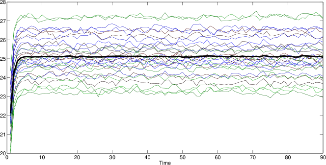
Figure 1: An example of mean-field control of space heaters. The light lines show the temperature of individual heaters and the thick line depicts the mean-field of the trajectories. Note that the individual trajectories adjust around their initial values so that the mean-field tracks the reference trajectory $z_{ref}=25$. The tracking is not perfect because of the friction between tracking the initial states locally and tracking the mean-field globally.

Define

$$\mathring{X}^{i}_{t} =\mathds{E}[\bar{X}^{i}_{t}\mid\mathbf{Y}_{1:t},\tilde{U}_{1:t-1},Z_{1:t}],$$

$$\breve{X}^{i}_{t} =\mathds{E}[X^{i}_{t}\mid\mathbf{Y}_{1:t},\tilde{U}_{1:t-1},Z_{1:t}].$$

Since $X^{i}_{t}=\bar{X}^{i}_{t}+Z_{t}$, we have that $\breve{X}^{i}_{t}=\mathring{X}^{i}_{t}+Z_{t}$.

From the Separation Theorem for linear quadratic Gaussian systems [15], we know that the optimal (centralized) control law for the auxiliary system is given by

$$\bar{U}^{i}_{t}=K^{x}_{t}\mathring{X}^{i}_{t},\quad U^{z}_{t}=K^{z}_{t}Z_{t},\quad i\in\{1,\ldots,N\}.$$

Or equivalently,

$$U^{i}_{t}=K^{x}_{t}\breve{X}^{i}_{t}+(K^{z}_{t}-K^{x}_{t})Z_{t},\quad i\in\{1,\ldots,n\}.$$

Thus, to prove Theorem 2, we need to show that $\breve{X}^{i}_{t}=\hat{X}^{i}_{t}$ (where $\hat{X}^{i}_{t}$ is defined in Theorem 2). This is proved below.

Lemma 2

In the auxiliary system with noisy observation, $\breve{X}^{i}_{t}=\hat{X}^{i}_{t}$. _□

Proof

Recall that $X^{i}_{t}$ evolves according to (1) and $Y^{i}_{t}$ is given by (3). Therefore, for any $i,j\in\{1,\dots,n\}$ such that $i\neq j$, $(X^{i}_{1:t},Y^{i}_{1:t})$ is conditionally independent of $(X^{j}_{1:t},Y^{j}_{1:t})$. Consequently,

$$\breve{X}^{i}_{t} =\mathds{E}[X^{i}_{t}\mid\mathbf{Y}_{1:t},\tilde{U}_{1:t-1},Z_{1:t}]$$

$$=\mathds{E}[X^{i}_{t}\mid Y^{i}_{1:t},\tilde{U}_{1:t-1},Z_{1:t}]$$

$$=\mathds{E}[X^{i}_{t}\mid Y^{i}_{1:t},\mathbf{U}_{1:t-1},Z_{1:t}]$$

$$\stackrel{{\scriptstyle(a)}}{{=}}\mathds{E}[X^{i}_{t}\mid Y^{i}_{1:t},U^{i}_{1:t-1},Z_{1:t}]$$

$$=\hat{X}^{i}_{t},$$

where $(a)$ follows because $X^{i}_{t}$ depends on $\mathbf{U}_{1:t-1}$ only through $U^{i}_{1:t-1}$.

_■

IV Numerical Example

We simulate an example of inspired by the collective target tracking mean-field model of [16]. We consider a population of space heaters. The state $X^{i}_{t}$ denotes the room temperature at heater $i$ at time $t$. We assume that the inital mean temperature is $z_{1}$ degrees, with individual temperatures distributed according to Gaussian distribution with unit variance around $z_{1}$ degrees. We assume that the temperature dynamics are linearized around the operating point and are given by

$$X^{i}_{t+1}=a(X^{i}_{t}-x_{0})+bU^{i}_{t}+W^{i}_{t}$$

where $x_{0}$ is the ambient temperature, $W^{i}_{t}$ is the randomness due to the environment and $U^{i}_{t}$ is the control action of a local controller.

It is desired that the mean temperature increases to 21 degrees (denoted by $z_{ref}$) in $T$ time steps (we assume $T=90$ minutes). The per-step cost function is

$$\frac{1}{n}\sum_{i=1}^{n}\Big{[}q(X^{i}_{t}-X^{i}_{1})^{2}+r{U^{i}_{t}}^{2}\Big{]}+p(Z_{t}-z_{ref})^{2}$$

The rationale of this cost function is as follows. It is assumed that the inital temperature is the comfort level of user $i$; so we penalize local deviations from the initial temperature. The second term corresponds to the local control energy. The last term is the penalty for the mean-field deviating from the reference mean-field. The objective is to minimize the expected total cost over a finite horizon.

The above model is a tracking problem. The results of Theorem 1 extend to tracking problems in a natural manner. We solve the Riccati equations for the following values of the parameters:

$$n =30, a =0.8, b =1,$$

$$q =0.5, p =1, r =1,$$

$$x_{0} =22, z_{1} =22, z_{ref} =25,$$

$$T =90, W^{i}_{t} \sim\mathcal{N}(0,1), X^{i}_{1} \sim\mathcal{N}(22,2).$$

The resultant trajectories are shown in Fig. 1.

V Conclusion

We consider team-optimal control of finite number of mean-field coupled LQG subsystems with mean-field sharing information structure. The optimal control law is unique, identical for all controllers, and linear in the current state and the current mean-field; the optimal gains are obtained by solving two decoupled Riccati equations for the full observation case and an additional filter Riccati equation for the noisy observation case. These Riccati equations do not depend on the number of subsystems.

To prove the main results, we consider an auxiliary centralized system whose dynamics and cost are equivalent to the original decentralized system. It is shown that the optimal centralized control law are implementable with mean-field sharing. Thus, the optimal decentralized control laws are identical to the optimal centralized control laws.

Although we only presented the results for the finite horizon optimal regulation problem, the results extend to infinte horizon and to optimal tracking problems in a natural manner. Moreover, it is possible to extend the results to non-homogeneous population consisting of multiple types.

References

- [1] M. Aicardi, F. Davoli, and R. Minciardi, “Decentralized optimal control of Markov chains with a common past information set,” IEEE Trans. Autom. Control, vol. 32, no. 11, pp. 1028–1031, 1987.
- [2] A. Nayyar, A. Mahajan, and D. Teneketzis, “Optimal control strategies in delayed sharing information structures,” IEEE Trans. Autom. Control, vol. 56, no. 7, pp. 1606–1620, Jul. 2011.
- [3] J. M. Ooi, S. M. Verbout, J. T. Ludwig, and G. W. Wornell, “A separation theorem for periodic sharing information patterns in decentralized control,” IEEE Trans. Autom. Control, vol. 42, no. 11, pp. 1546–1550, Nov. 1997.
- [4] S. Yüksel, “Stochastic nestedness and the belief sharing information pattern,” IEEE Trans. Autom. Control, pp. 2773–2786, Dec. 2009.
- [5] J. Arabneydi and A. Mahajan, “Team optimal control of coupled subsystems with mean field sharing,” in Proc. 53rd IEEE Conf. Decision and Control, Los Angeles, CA, Dec. 2014, pp. 1669–1674.
- [6] A. Nayyar, A. Mahajan, and D. Teneketzis, “Decentralized stochastic control with partial history sharing: A common information approach,” IEEE Trans. Autom. Control, vol. 58, no. 7, pp. 1644–1658, Jul. 2013.
- [7] A. Mahajan, N. Martins, M. Rotkowitz, and S. Yüksel, “Information structures in optimal decentralized control,” in Proc. 51st IEEE Conf. Decision and Control, Maui, Hawaii, Dec. 2012, pp. 1291 – 1306.
- [8] M. Huang, P. Caines, and R. Malhame, “Large population cost-coupled LQG problems with non-uniform agents: individual mass behavior and decentralized epsilon-nash equilibrium,” IEEE Trans. Autom. Control, vol. 52, no. 9, pp. 1560–1571, Sep. 2007.
- [9] ——, “An invariance principle in large population stochastic dynamic games,” Journal of Systems Science and Complexity, vol. 20, pp. 162–172, 2007.
- [10] P. Lions and J. Larsy, “Mean-field games,” Japanese Journal of Mathematics, vol. 2, no. 1, pp. 229–260, Mar. 2007.
- [11] T. Li and J.-F. Zhang, “Asymptotically optimal decentralized control for large population stochastic multiagent systems,” IEEE Trans. Autom. Control, vol. 53, no. 7, pp. 1643–1660, 2008.
- [12] O. Guéant, J.-M. Lasry, and P.-L. Lions, Paris-Princeton Lecture on Mathematical Finance. Springer, 2011, ch. Mean-field games and applications, pp. 205–266.
- [13] M. Huang, P. E. Caines, and R. P. Malhamé, “Social optima in mean field LQG control: centralized and decentralized strategies,” IEEE Trans. Autom. Control, vol. 57, no. 7, pp. 1736–1751, 2012.
- [14] R. Elliott, X. Li, and Y.-H. Ni, “Discrete time mean-field stochastic linear-quadratic optimal control problems,” Automatica, vol. 49, no. 11, pp. 3222–3233, 2013.
- [15] P. E. Caines, Linear stochastic systems. John Wiley & Sons, Inc., 1987.
- [16] A. Kizilkale and R. Malhame, “Mean field based control of power system dispersed energy storage devices for peak load relief,” in IEEE Conference on Decision and Control (CDC), Dec. 2013, pp. 4971–4976.