Reinforcement Learning in Decentralized Stochastic Control Systems with Partial History Sharing

Abstract

In this paper, we are interested in systems with multiple agents that wish to collaborate in order to accomplish a common task while a) agents have different information (decentralized information) and b) agents do not know the model of the system completely i.e., they may know the model partially or may not know it at all. The agents must learn the optimal strategies by interacting with their environment i.e., by decentralized Reinforcement Learning (RL). The presence of multiple agents with different information makes decentralized reinforcement learning conceptually more difficult than centralized reinforcement learning. In this paper, we develop a decentralized reinforcement learning algorithm that learns $\epsilon$-team-optimal solution for partial history sharing information structure, which encompasses a large class of decentralized control systems including delayed sharing, control sharing, mean field sharing, etc. Our approach consists of two main steps. In the first step, we convert the decentralized control system to an equivalent centralized POMDP (Partially Observable Markov Decision Process) using an existing approach called common information approach. However, the resultant POMDP requires the complete knowledge of system model. To circumvent this requirement, in the second step, we introduce a new concept called “Incrementally Expanding Representation” using which we construct a finite-state RL algorithm whose approximation error converges to zero exponentially fast. We illustrate the proposed approach and verify it numerically by obtaining a decentralized Q-learning algorithm for two-user Multi Access Broadcast Channel (MABC) which is a benchmark example for decentralized control systems.

Proceedings of American Control Conference, 2015.

1 INTRODUCTION

1.1 Motivation

Decentralized decision making is relevant in a wide range of applications ranging from networked control systems, robotics, transportation networks, communication networks, sensor networks, and economics. There is a rich history of research on optimal stochastic control of decentralized system. We refer the reader to [1] for a detailed review.

Most of the literature assumes that the system model is completely known to all decision makers; however, in practice, such knowledge may only be available partially or may not be available. Hence, it is crucial for decision makers to be able to learn the optimal solutions. In the literature, learning in centralized stochastic control is well studied and there exist many approaches such as model-predictive control, adaptive control, and reinforcement learning. This is in contrast to the learning in decentralized stochastic control; it is not immediately clear on how centralized learning approaches would work for decentralized systems. In this paper, we propose a novel Reinforcement Learning (RL) algorithm for a class of decentralized stochastic control systems that guarantees team-optimal solution.

Existing approaches for multi-agent learning may be categorized as follows: exact methods and heuristics. The exact methods rely on the assumption that the information structure is such that all agents can consistently update the Q-function. These include approaches that rely on social convention and rules to restrict the decisions made by the agents [10]; approaches that use communication to convey the decisions to all agents [11]; and approaches that assume that the Q-function decomposes into a sum of terms, each of which is independently updated by an agent [12]. Heuristic approaches include joint action learners heuristic [13], where each agent learns the empirical model of the system in order to estimate the control action of other agents; frequency maximum Q-value heuristic [14], where agents keep track of the frequency with which each action leads to a “good” outcome; heuristic Q-learning [15], which assigns a rate of punishment for each agent; and distributed Q-learning [16], which uses predator-prey models to assign heuristic sub-goals to individual agents. To the best of our knowledge, there is no RL approach that guarantees team-optimal solution. In this paper, we present such an approach.

We describe the system model and problem formulation in Sections 1.3 and 1.4, respectively. We state the main challenges in Section 1.5 and our main contributions in Section 1.6. In Section 2, we present a brief preliminary on Partial History Sharing (PHS) information structure. We describe our approach in two basic steps in Section 3. In Section 4, we mention a few points on the implementation. Based on the proposed approach, we develop a RL algorithm for a benchmark example with numerical results in Section 5.

1.2 Notation

We use upper-case letters to denote random variables (e.g. $X$) and lower-case letters to denote their realizations (e.g. $x$). We use the short-hand notation $X_{a:b}$ for the vector $(X_{a},X_{a+1},\ldots,X_{b})$ and bold letters to denote vectors e.g. $\mathbf{Y}=(Y^{1},\ldots,Y^{n})$. $\mathbb{P}(\cdot)$ is the probability of an event, $\mathbb{E}[\cdot]$ is the expectation of a random variable, and $|\cdot|$ is the absolute value of a real number. $\mathbb{N}$ refers to the set of natural numbers and $\mathbb{Z}^{+}=\mathbb{N}\cup\{0\}$.

1.3 System Model

Let $X_{t}\in\mathcal{X}$ denote the state of a dynamical system controlled by $n$ agents. At time $t$, agent $i$ observes $Y^{i}_{t}\in\mathcal{Y}^{i}$ and chooses $U^{i}_{t}\in\mathcal{U}^{i}$. For ease of notation, we denote the joint actions and the joint observations by $\mathbf{U}_{t}=(U^{1}_{t},\ldots,U^{n}_{t})\in\mathcal{U}$ and $\mathbf{Y}_{t}=(Y^{1}_{t},\ldots,Y^{n}_{t})\in\mathcal{Y}$, respectively. The dynamics of the system are given by

$$X_{t+1}=f(X_{t},\mathbf{U}_{t},W^{s}_{t}),\vspace{-.2cm}$$ (1)

and the observations are given by

$$\mathbf{Y}_{t}=h(X_{t},\mathbf{U}_{t-1},W^{o}_{t}),\vspace{-.2cm}$$ (2)

where $\{W^{s}_{t}\}_{t=1}^{\infty}$ is an i.i.d. process with probability distribution function $P_{W^{s}}$, $\{W^{o}_{t}\}_{t=1}^{\infty}$ is an i.i.d. process with probability distribution function $P_{W^{o}}$, and $X_{1}$ is the initial state with probability distribution function $P_{X}$. The primitive random variables $\{X_{1},\{W^{s}_{t}\}_{t=1}^{\infty},\{W^{o}_{t}\}_{t=1}^{\infty}\}$ are mutually independent and defined on a common probability space.

For ease of exposition, we assume all system variables are finite valued. Let $I^{i}_{t}\subseteq\{\mathbf{Y}_{1:t},\mathbf{U}_{1:t-1}\}$ be information available at agent $i$ at time $t$. The collection $(\{I^{i}_{t}\}_{t=1}^{\infty},i=1,\ldots,n)$ is called the information structure. In this paper, we restrict attention to an information structure called partial history sharing [2], which will be defined later.

At time $t$, agent $i$ chooses action $U^{i}_{t}$ according to control law $g^{i}_{t}$ as follows

$$U^{i}_{t}=g^{i}_{t}(I^{i}_{t}).\vspace{-.1cm}$$ (3)

We denote $\bm{g}^{i}=(g^{i}_{1},g^{i}_{2},\ldots)$ as strategy of agent $i$ and $\bm{g}=(\bm{g}^{1},\ldots,\bm{g}^{n})$ as joint strategy of all the agents. The performance of strategy $\mathbf{g}$ is measured by the following infinite-horizon discounted cost

$$J(\bm{g})=\mathbb{E}^{\bm{g}}\left[\sum_{t=1}^{\infty}\beta^{t-1}\ell(X_{t},\mathbf{U}_{t})\right],$$ (4)

where $\beta\in(0,1)$ is the discount factor, $\ell$ is the per-step cost function, and the expectation is with respect to a joint probability distribution on $(X_{1:\infty},\mathbf{U}_{1:\infty})$ induced by the joint probability distribution on the primitive random variables and the choice of strategy $\bm{g}$.

A strategy $\bm{g}^{\ast}$ is optimal if for any other strategy $\bm{g}$, $J(\bm{g}^{\ast})\leq J(\bm{g}).$ For $\epsilon>0$, strategy $\bm{g}^{\ast}$ is $\epsilon$-optimal, if for any other strategy $\bm{g}$, $J(\bm{g}^{\ast})\leq J(\bm{g})+\epsilon.$

1.4 Problem Formulation

We will consider three different setups that differ in the assumptions about the knowledge of the model. For all the setups, we will assume that the action and the observation spaces as well as the information structure, the discount factor $\beta$, and an upper-bound on the per-step cost are common knowledge between all agents. The setups differ in the assumptions about state space $\mathcal{X}$, system dynamics and observations ($f,h$), probability distributions ($P_{X},P_{W^{s}},P_{W^{o}}$), and cost structure $\ell$. These include two setups, 1) complete-knowledge of the model, and 2) incomplete-knowledge of the model which includes two sub-cases: 2a) partial-knowledge of the model and 2b) no-knowledge of the model.

In general, the complete-knowledge of the model is required to find an optimal strategy $\bm{g}^{\ast}$. However, in practice, there are many applications where such information is not completely available or is not available at all. In such applications, the agents must learn the optimal strategy by interacting with their environment. This is known as reinforcement learning (RL). If the agents have partial knowledge of the model, the setup is called model-based RL. If the agents have no knowledge of the model, setup is called model-free RL.

Define $L:=\max_{x,\mathbf{u}}|\ell(x,\mathbf{u})|$. We are interested in the following problem.

Problem 1.

Given the information structure, action spaces $\{\mathcal{U}^{i}\}_{i=1}^{n}$, observation spaces $\{\mathcal{Y}^{i}\}_{i=1}^{n}$, discount factor $\beta$, the upper-bound $L$ on per-step cost, and any $\epsilon>0$, develop a (model-based or model-free) reinforcement learning algorithm using which the agents learn an $\epsilon$-optimal strategy $\bm{g}^{\ast}$.

1.5 Main Difficulties

Given the complete knowledge of system model, finding team-optimal solution in decentralized control systems is conceptually challenging due to the decentralized nature of information available to the agents. The agents need to cooperate with each other to fulfill a common objective while they have different perspectives about themselves, other agents, and the environment. This discrepancy in perspectives makes establishing cooperation among agents difficult; we refer reader to [21] for details. Thus, finding team-optimal solution is even more challenging when agents have only partial knowledge or no knowledge of system model. Hence, it is difficult to consistently learn strategies in such settings.

1.6 Contributions

Below, we mention our main contributions in this paper.

1) We propose a novel approach to perform reinforcement learning in a large class of decentralized stochastic control systems with partial history sharing (PHS) information structure that guarantees $\epsilon$-team-optimal solution. In particular, our approach combines the common information approach of [2] with any RL algorithm of Partially Observable Markov Decision Processes (POMDP). The approach works in two steps. In the first step, the common information approach is used to convert the decentralized control problem to an equivalent centralized POMDP and in the second step, a RL algorithm is used to provide a learning scheme to identify an $\epsilon$-optimal strategy in the resultant POMDP. Note that any RL algorithm of POMDPs may be used in the second step; however, we develop a new methodology for the second step as explained below.

2) We propose a novel methodology to perform reinforcement learning in centralized POMDPs as an intermediate step of the two-step approach described above. (This methodology by itself may be of interest due to the fact that developing RL algorithm in POMDPs is difficult). The methodology consists of three parts: 1) converting the POMDP to a countable-state MDP $\Delta$ by defining a new concept that we call Incrementally Expanding Representation (IER), 2) approximating $\Delta$ with a sequence of finite-state MDPs $\{\Delta_{N}\}_{N=1}^{\infty}$, and 3) using a RL algorithm to learn an optimal strategy of MDP $\Delta_{N}$. We show that the performance of the RL strategy converges to the optimal performance exponentially as $N\rightarrow\infty$. We use this methodology in the second step of the two-step approach.

3) Using the proposed two-step approach, we develop a RL algorithm for two-user Multi Access Broadcast Channel (MABC) which is used as a benchmark for decentralized control systems. Numerical simulations validate that the RL algorithm converges to an optimal strategy.

2 Preliminaries on Partial History Sharing

Herein, we present a simplified version of partial history sharing information structure, originally presented in [2].

Definition 1 ([2], Partial History Sharing (PHS)).

Consider a decentralized control system with $n$ agents. Let $I^{i}_{t}$ denote the information available to agent $i$ at time $t$. Assume $I^{i}_{t}\subseteq I^{i}_{t+1}$. Then, split the information at each agent into two parts: common information $C_{t}=\bigcap_{i=1}^{n}I^{i}_{t}$ i.e. the information shared between all agents and local information $M^{i}_{t}=I^{i}_{t}\backslash C_{t}$ that is the local information of agent $i$. Define $Z_{t}:=C_{t+1}\backslash C_{t}$ as common observation, then $C_{t+1}=Z_{1:t}$. An information structure is called partial history sharing when the following conditions are satisfied:

1. The update of local information

   $$M^{i}_{t+1}\subseteq\{M^{i}_{t},U^{i}_{t},Y^{i}_{t+1}\}\backslash Z_{t},\quad i\in\{1,\ldots,n\}.$$

2. For every agent $i$, the size of the local information $M^{i}_{t}$ and the size of the common observation $Z_{t}$ are uniformly bounded in time $t$.

These conditions are fairly mild and are satisfied by a large class of models. Examples include delayed sharing [17], periodic sharing [18], mean-field sharing [19], etc. Even for models that do not satisfy the above conditions directly, it is often possible to identify sufficient statistics that satisfy the above conditions, e.g., control sharing [20].

Remark 1.

Note that the conditions (a) and (b) are valid even if there is no common information between agents i.e., $C_{t}=\emptyset$. Hence, the decentralized control systems with pure decentralized information (i.e. no information commonly shared) falls into PHS information structure.

3 Approach

In this part, we derive a RL algorithm for systems with PHS information structure. Our approach consists of two steps. In the first step, we consider the setup of the complete-knowledge of the model and use the common information approach of [2] to convert the decentralized control problem to an equivalent centralized POMDP. In the second step, we consider the setup of incomplete-knowledge of the model and develop a finite-state RL algorithm based on the POMDP obtained in the first step.

3.1 Step 1: An Equivalent Centralized POMDP

In this section, we present common information approach of [2] and its main results for the setup of complete-knowledge of the model described in Section 1.3.

Let $\mathcal{M}^{i}$ and $\mathcal{Z}$ denote the spaces of realizations of local information of agent $i$ and common observation, respectively. Consider a virtual coordinator that observes the common information $C_{t}$ shared between all agents and chooses $(\Gamma^{1}_{t},\ldots,\Gamma^{n}_{t})$, where $\Gamma^{i}_{t}:\mathcal{M}^{i}\mapsto\mathcal{U}^{i}$ is the mapping from the local information of agent $i$ to action of agent $i$ at time $t$, according to

$$\Gamma^{i}_{t}=\psi^{i}_{t}(C_{t}),\quad i\in\{1,\ldots,n\}.\vspace{-.1cm}$$ (5)

We call $\bm{\psi}_{t}:=\{\psi^{1}_{t},\ldots,\psi^{n}_{t}\}$ the coordination law and $\bm{\Gamma}_{t}=(\Gamma^{1}_{t},\ldots,\Gamma^{n}_{t})$ the prescription. The agents use this prescription to choose their actions as follows:

$$U^{i}_{t}=\Gamma^{i}_{t}(M^{i}_{t}),\quad i\in\{1,\ldots,n\}.\vspace{-.1cm}$$ (6)

We denote the space of mappings $\Gamma^{i}_{t}$ by $\mathcal{G}^{i}$ and the space of prescriptions $\mathbf{\Gamma}_{t}$ by $\mathcal{G}=\prod_{i=1}^{n}\mathcal{G}^{i}$. In the sequel, for ease of notation, we will use the following compact form for the coordinator’s law,

$$\bm{\Gamma}_{t}=\bm{\psi}_{t}(C_{t}).\vspace{-.1cm}$$ (7)

We call $\bm{\psi}=\{\bm{\psi}_{1},\bm{\psi}_{2},\ldots\}$ as the coordination strategy. In the coordinated system, dynamics and cost function are as same as those in the original problem in Section 1.3. In particular, the infintie-horizon discounted cost in the coordinated system is as follows:

$$J(\bm{\psi})=\mathbb{E}^{\bm{\psi}}\left[\sum_{t=1}^{\infty}\beta^{t-1}\ell(\mathbf{X}_{t},\bm{\Gamma}^{1}_{t}(M^{1}_{t}),\ldots,\Gamma^{n}_{t}(M^{n}_{t}))\right].$$ (8)

Lemma 1 ([2], Proposition 3).

The original system described in Section 1.3 with PHS information structure is equivalent to the coordinated system.

We denote $\bm{M}_{t}=(M^{1}_{t},\ldots,M^{n}_{t})$ as the joint local information. According to [2], $\Pi_{t}=\mathbb{P}(X_{t},\mathbf{M}_{t}|Z_{1:t-1},\bm{\Gamma}_{1:t-1})$ is an information state for the coordinated system. It is shown in [2] that:

1. There exists a function $\phi$ such that

   $$\Pi_{t+1}=\phi(\Pi_{t},\bm{\Gamma}_{t},Z_{t}).\vspace{-.1cm}$$ (9)

2. The observation $Z_{t}$ only depends on $(\Pi_{t},\Gamma_{t})$ i.e.

   $$\mathbb{P}(Z_{t}|\Pi_{1:t},\bm{\Gamma}_{1:t})=\mathbb{P}(Z_{t}|\Pi_{t},\bm{\Gamma}_{t}).\vspace{-.1cm}$$ (10)

3. There exists a function $\hat{\ell}$ such that

   $$\hat{\ell}(\pi_{t},\bm{\gamma}_{t})=\mathbb{E}[\ell(X_{t},\mathbf{U}_{t}|Z_{1:t-1}=z_{1:t-1},\bm{\Gamma}_{1:t}=\bm{\gamma}_{1:t})].\vspace{-.1cm}$$ (11)

Assume that the initial state $\pi_{1}$ is fixed. Let $\mathcal{R}$ denote the reachable set of above centralized POMDP that contains all the realizations of $\pi_{t}$ generated by $\pi_{t+1}=\phi(\pi_{t},\bm{\gamma},z),\forall\bm{\gamma}\in\mathcal{G},\forall z\in\mathcal{Z},\forall t\in\mathbb{N}$, with initial information state $\pi_{1}$. Note that since all the variables are finite valued, then $\mathcal{G}$ (set of all prescriptions $\bm{\gamma}$) and $\mathcal{Z}$ (set of all observations of the coordinator) are finite sets. Hence, $\mathcal{R}$ is at most a countable set.

Theorem 1 ([2], Theorem 5).

Let $\bm{\psi}^{\ast}(\pi)$ be any argmin of the right-hand side of following dynamic program. For $\pi\in\mathcal{R}$,

$$V(\pi)=\min_{\bm{\gamma}}(\hat{\ell}(\pi,\bm{\gamma})+\beta\mathbb{E}[V(\phi(\pi,\bm{\gamma},Z_{t}))|\Pi_{t}=\pi,\bm{\Gamma}_{t}=\bm{\gamma}]),\vspace{-.1cm}$$

where $\bm{\gamma}=(\gamma^{1},\ldots,\gamma^{n})$ and the minimization is over all functions $\gamma^{i}\in\mathcal{G}^{i},i\in\{1,\ldots,n\}$. Then, the joint stationary strategy $\bm{g}^{\ast}=(\bm{g}^{1,\ast},\ldots,\bm{g}^{n,\ast})$ is optimal such that

$$g^{i,\ast}(\pi,m^{i}):=\bm{\psi}^{i,\ast}(\pi)(m^{i}),\quad\pi\in\mathcal{R},m^{i}\in\mathcal{M}^{i},\forall i.$$

In the next step, we develop a finite-state RL algorithm based on the obtained POMDP for the setup of incomplete-knowledge of the model.

3.2 Step 2: Finite-State RL Algorithm For POMDP

In the previous step, we identified a centralized POMDP that is equivalent to the decentralized control system with PHS information structure. However, the obtained POMDP requires the complete knowledge of the model. To circumvent this requirement, we introduce a new concept that we call Incrementally Expanding Representation (IER). The main feature of IER is to remove the dependency of the POMDP from the complete knowledge of the model. Based on a proper IER, in this step, we develop a finite-state RL algorithm. This step consists of three parts. In part (1), we convert the POMDP to a countable-state MDP $\Delta$ without loss of optimality. In part (2), we construct a sequence of finite-state MDPs $\{\Delta_{N}\}_{N=1}^{\infty}$ of MDP $\Delta$. In part (3), we use a generic RL algorithm to learn an optimal strategy of $\Delta_{N}$.

Definition 2 (Incrementally Expanding Representation).

Let $\{\mathcal{S}_{k}\}_{k=1}^{\infty}$ be a sequence of finite sets such that $\mathcal{S}_{1}\subsetneq\mathcal{S}_{2}\subsetneq\ldots\subsetneq\mathcal{S}_{k}\subsetneq\ldots$, and $\mathcal{S}_{1}$ is a singleton, say $\mathcal{S}_{1}=\{s^{\ast}\}$. Let $\mathcal{S}=\lim_{k\rightarrow\infty}\mathcal{S}_{k}$ be the countable union of above finite sets, $B:\mathcal{S}\rightarrow\mathcal{R}$ be a surjective function that maps $\mathcal{S}$ to the reachable set $\mathcal{R}$, and $\tilde{f}:\mathcal{S}\times\mathcal{G}\times\mathcal{Z}\rightarrow\mathcal{S}$. The tuple $\langle\{\mathcal{S}_{k}\}_{k=1}^{\infty},B,\tilde{f}\rangle$ is called an Incrementally Expanding Representation (IER), if it satisfies the following properties:

(P1) Incremental Expansion: For any $\bm{\gamma}\in\mathcal{G},z\in\mathcal{Z},$ and $s\in\mathcal{S}_{k}$, we have that

$$\tilde{f}(s,\bm{\gamma},z)\in\mathcal{S}_{k+1}.\vspace{-.1cm}$$ (12)

(P2) Consistency: For any $(\bm{\gamma}_{1:t-1},z_{1:t-1})$, let $\pi_{t}$ and $s_{t}$ be the states obtained by recursive application of (9) and (12) starting from $\pi_{1}$ and $``s^{\ast}$, respectively. Then,

$$\pi_{t}=B(s_{t}).\vspace{-.1cm}$$ (13)

In general, every decentralized control system with PHS information structure has at least one IER. In the following example, we present a generic IER that is valid for every system with PHS information structure.

Example 1: Let $S_{1}=\{\emptyset\}$, $S_{2}=\{\emptyset\}\cup\{\mathcal{G}\times\mathcal{Z}\}$, and $S_{k+1}=S_{k}\cup\{\mathcal{G}\times\mathcal{Z}\}^{k},k\in\mathbb{N}$. Let $S=\lim_{k\rightarrow\infty}S_{k}$ and $B:\mathcal{S}\rightarrow\mathcal{R}$ such that

$$B(\emptyset)=\pi_{1},B(s_{k+1})=\phi(\phi(....,\bm{\gamma}_{k-1},z_{k-1}),\bm{\gamma}_{k},z_{k})=\pi_{k+1},\vspace{-.1cm}$$

where $s_{k+1}=((\bm{\gamma}_{1},z_{1}),\ldots,(\bm{\gamma}_{k},z_{k}))\in\mathcal{S}_{k+1}$. Define $\tilde{f}$ as follows:

$$\tilde{f}(s,\bm{\gamma},z)=s\circ\bm{\gamma}\circ z,$$

where $\circ$ denotes concatenation. By construction, tuple $\langle\{\mathcal{S}_{k}\}_{k=1}^{\infty},B,\tilde{f}\rangle$ satisfies (P1) and (P2), and hence is an IER.

3.21 Countable-state MDP $\Delta$

Let the tuple $\langle\{\mathcal{S}_{k}\}_{k=1}^{\infty},B,\tilde{f}\rangle$ be an IER of the POMDP obtained in the first step. Then, define MDP $\Delta$ with countable state space $\mathcal{S}$, finite action space $\mathcal{G}$, and dynamics $\tilde{f}$ such that:

(F1) The initial state is singleton $s^{\ast}$. The state $S_{t}\in\mathcal{S}_{k}$, $k\leq t$, evolves as follows: for $\bm{\Gamma}_{t}\in\mathcal{G},Z_{t}\in\mathcal{Z},$

$$S_{t+1}=\tilde{f}(S_{t},\bm{\Gamma}_{t},Z_{t}),\quad S_{t+1}\in\mathcal{S}_{k+1}$$ (14)

where observation $Z_{t}$ only depends on $(S_{t},\bm{\Gamma}_{t})$ (that is a consequence of (10) and consistency property in (13)). At time $t$, there is a cost depending on the current state $S_{t}\in\mathcal{S}$ and action $\bm{\Gamma}_{t}\in\mathcal{G}$ given by

$$\tilde{\ell}(S_{t},\bm{\Gamma}_{t}):=\hat{\ell}(B(S_{t}),\bm{\Gamma}_{t})=\hat{\ell}(\Pi_{t},\bm{\Gamma}_{t}).\vspace{-.1cm}$$ (15)

(F2) State space $\mathcal{S}$, action space $\mathcal{G}$, and dynamics $\tilde{f}$ do not depend on the unknowns.

The performance of a stationary strategy $\tilde{\bm{\psi}}:\mathcal{S}\mapsto\mathcal{G}$ is quantified by

$$\tilde{J}(\tilde{\bm{\psi}})=\mathbb{E}^{\tilde{\bm{\psi}}}\left[\sum_{t=1}^{\infty}\beta^{t-1}\tilde{\ell}(S_{t},\bm{\Gamma}_{t})\right].$$ (16)

There may exist more than one IER that satisfy above features. For instance, the IER of Example 1 always satisfies (F1) and (F2) (that is model-free). This IER can also be used in the model-based cases; however, in the model-based cases, due to having partial knowledge of the model, one may be able to find a simpler IER. See Section 5 for an example.

Lemma 2.

Let $\tilde{\bm{\psi}^{\ast}}$ be an optimal strategy for MDP $\Delta$. Construct a strategy $\bm{\psi}^{\ast}$ for the coordinated system as follows:

$$\tilde{\bm{\psi}^{\ast}}(s)=:\bm{\psi}^{\ast}(B(s)),\quad\forall s\in\mathcal{S}.$$ (17)

Then, $\tilde{J}(\tilde{\bm{\psi}^{\ast}})=J(\bm{\psi}^{\ast})$ and $\bm{\psi}^{\ast}$ is an optimal strategy for the coordinated system, and therefore can be used to generate an optimal strategy for the decentralized control system.

Proof is omitted due to lack of space.

3.22 Finite-state incrementally expanding MDP $\Delta_{N}$

In this part, we construct a series of finite-state MDPs $\{\Delta_{N}\}_{N=1}^{\infty}$, that approximate the countable-state MDP $\Delta$ as follows. Let $\Delta_{N}$ be a finite-state MDP with state space $\mathcal{S}_{N}$ and action space $\mathcal{G}$. The transition probability of $\Delta_{N}$ is constructed as follows. Pick any arbitrary set $D^{\ast}\in S_{N}$. Remap every transition in $\Delta$ that takes the state $s\in\mathcal{S}_{N}$ to $s^{\prime}\in\mathcal{S}_{N+1}\backslash\mathcal{S}_{N}$ to a transition from $s\in\mathcal{S}_{N}$ to any (not necessarily unique) state in $D^{\ast}$. In addition, the per-step cost function of $\Delta_{N}$ is simply a restriction of $\tilde{\ell}$ to $\mathcal{S}_{N}\times\mathcal{G}$.

We assume that there exists an action or a sequence of actions that if taken, the system transmits to a known state $d^{\ast}$ in $D^{\ast}$. For example, suppose there is a reset action in the system. After executing the reset action, the state of the system is reset and transmitted to a known state $d^{\ast}\in D^{\ast}$. Let $\tau_{N}\in\mathbb{N}$ be the longest amount of time during which $S_{t}$, $t\leq\tau_{N}$, stays in $\mathcal{S}_{N}$ under dynamics $\tilde{f}$, optimal strategy $\tilde{\bm{\psi}^{\ast}}$, and any arbitrary sample path of $z_{1:\tau_{N}-1}$, i.e.,

$$S_{t}=\tilde{f}(S_{t-1},\tilde{\bm{\psi}^{\ast}}(S_{t-1}),Z_{t-1})\in\mathcal{S}_{N},\quad\forall t\leq\tau_{N}.$$ (18)

Let $\tilde{\bm{\psi}_{N}^{\ast}}$ and $\tilde{J}_{N}(\tilde{\bm{\psi}_{N}^{\ast}})$ be an optimal stationary strategy of $\Delta_{N}$ and the optimal cost (performance) of $\Delta_{N}$, respectively.

Theorem 2.

The difference in performance between $\Delta$ and $\Delta_{N}$ is bounded as follows:

$$|\tilde{J}(\tilde{\bm{\psi}^{\ast}})-\tilde{J}_{N}(\tilde{\bm{\psi}_{N}^{\ast}})|\leq\frac{2\beta^{\tau_{N}}}{1-\beta}L.$$ (19)

Proof is omitted due to lack of space.

The upper-bound provided in Theorem 2 requires knowledge on $(\tilde{f}$, $\tilde{\bm{\psi}^{\ast}}$,$\mathcal{Z})$. However, according to (14), $\tau_{N}$ is always equal or greater than $N$ i.e. $N\leq\tau_{N}$. Hence, one can obtain a more conservative error-bound (larger upper-bound) than the error-bound (upper-bound) in Theorem 2 that does not require any knowledge on $(\tilde{f}$, $\tilde{\bm{\psi}^{\ast}}$,$\mathcal{Z})$ as follows.

Corollary 1.

The difference in performance between $\Delta$ and $\Delta_{N}$ is bounded as follows:

$$|\tilde{J}(\tilde{\bm{\psi}^{\ast}})-\tilde{J}_{N}(\tilde{\bm{\psi}_{N}^{\ast}})|\leq\frac{2\beta^{N}}{1-\beta}L.\vspace{-.0cm}$$ (20)

3.23 Finite-state RL algorithm

Let $\mathcal{T}$ be a generic (model-based or model-free) RL algorithm designed for finite-state MDPs with infinite horizon discounted cost. By a generic RL algorithm, we mean any algorithm which fits to the following framework. At each iteration $k\in\mathbb{N}$, $\mathcal{T}$ knows the state of system, selects one action, and observes an instantaneous cost and the next state. The strategy learned (generated) by $\mathcal{T}$ converges to an optimal strategy as $k\rightarrow\infty$.

Let $\mathcal{T}$ operate on MDP $\Delta_{N}$ such that, at iteration $k$, it knows the state of the system $s_{k}\in\mathcal{S}_{N}$, selects one action $\bm{\gamma}_{k}\in\mathcal{G}$, and observes an instantaneous cost $\ell_{k}$ (which is a realization of the incurred cost $\ell(X_{k},\mathbf{U}_{k})$ at the original decentralized system). According to (11) and (15), we have

$$\mathbb{E}[\ell(X_{k},\mathbf{U}_{k})|S_{1:k},\bm{\Gamma}_{1:k}]=\tilde{\ell}(S_{k},\bm{\Gamma}_{k}),\quad S_{k}\in\mathcal{S}_{N}.\vspace{-.1cm}$$ (21)

Hence, the instantaneous cost $\ell_{k}$ may be interpreted as a realization of the per-step cost of $\Delta_{N}$. Given dynamics $\tilde{f}$, $\mathcal{T}$ observes $z_{k}\in\mathcal{Z}$ and computes the next state $s_{k+1}=\tilde{f}(s_{k},\bm{\gamma}_{k},z_{k}).$ If $s_{k+1}\in\mathcal{S}_{N+1}\backslash\mathcal{S}_{N}$, then an action (or a sequence of actions) that transmits the state of system to a known state in $S_{N}$ i.e. $s_{k+1}=d^{\ast}\in D^{\ast}$ will be taken; otherwise, the system will continue from $s_{k+1}\in\mathcal{S}_{N}$.

Let $\tilde{\bm{\psi}}_{N}^{k}:\mathcal{S}_{N}\rightarrow\mathcal{G}$ be the learned strategy associated with RL algorithm $\mathcal{T}$ operating on MDP $\Delta_{N}$ at iteration $k$. Then, $\mathcal{T}$ updates its strategy $\tilde{\bm{\psi}}^{k+1}_{N}$ based on the observed cost $\ell_{k}$ and the transmitted next state $s_{k+1}$ by executing action $\bm{\gamma}_{k}$ at state $s_{k}$. We assume $\mathcal{T}$ converges to an optimal strategy $\tilde{\bm{\psi}^{\ast}_{N}}$ as $k\rightarrow\infty$ such that

$$\lim_{k\rightarrow\infty}|\tilde{J}_{N}(\tilde{\bm{\psi}}_{N}^{k})-\tilde{J}_{N}(\tilde{\bm{\psi}_{N}^{\ast}})|=0.\vspace{-.1cm}$$ (22)

Now, we need to convert (translate) the strategies in $\Delta_{N}$ to strategies in the original decentralized control problem described in Section 1.3, where the actual learning happens. Hence, we define a strategy $\bm{g}_{N}^{k}:=(g_{N}^{k,i},\ldots,g_{N}^{k,n})$, at iteration $k$, as follows:

$$g^{k,i}_{N}(s,m^{i}):=\tilde{\bm{\psi}}_{N}^{k,i}(s)(m^{i}),\forall s\in\mathcal{S}_{N},\forall m^{i}\in\mathcal{M}^{i},\forall i,$$ (23)

where $\tilde{\bm{\psi}}_{N}^{k,i}$ denotes the $i$th term of $\tilde{\bm{\psi}}_{N}^{k}$.

Algorithm 1     Finite-State RL Algorithm

1:Given $\epsilon>0$, choose a sufficiently large $N\in\mathbb{N}$ such that $\frac{2\beta^{N}}{1-\beta}L\leq\epsilon$. Then, construct state space $\mathcal{S}_{N}$, action space $\mathcal{G}$, and dynamics $\tilde{f}$. Initialize $s_{1}=s^{\ast}$.

2:At iteration $k\in\mathbb{N}$, RL algorithm $\mathcal{T}$ picks $\bm{\gamma}_{k}=(\gamma^{1}_{k},\ldots,\gamma^{n}_{k})\in\mathcal{G}$ at state $s_{k}\in\mathcal{S}_{N}$. Then, agent $i\in\{1,\ldots,n\}$ takes action $u^{i}_{k}$ according to the chosen prescription $\gamma^{i}_{k}$ and local information $m^{i}_{k}\in\mathcal{M}^{i}$ as follows:

$$u^{i}_{k}=\gamma^{i}_{k}(m_{k}^{i}),\quad\forall i.\vspace{-.1cm}$$

3:Based on the taken actions, the system incurs a cost $\ell_{k}$, evolves, and generates new information i.e. $(\{m^{i}_{k+1}\}_{i=1}^{n},z_{k})$. Every agent $i$ observes $z_{k}$ because it is common observation. Based on $z_{k}$, all agents consistently compute the next state

$$s_{k+1}=\tilde{f}(s_{k},\bm{\gamma}_{k},z_{k}).\vspace{-.1cm}$$

If $s_{k+1}\notin\mathcal{S}_{N}$, then agents take an action (or a sequence of actions) that transmits the state of system to a state $s_{k+1}=d^{\ast}\in\mathcal{S}_{N}$; otherwise, the system proceeds from $s_{k+1}\in\mathcal{S}_{N}$. Note that during the reset process, the algorithm is paused till the system lands in a state in $S_{N}$.

4:$\mathcal{T}$ updates its strategy from $\tilde{\bm{\psi}}_{N}^{k}$ to $\tilde{\bm{\psi}}_{N}^{k+1}$ based on performing action $\bm{\gamma}_{k}$ at state $s_{k}$ and transmission to next state $s_{k+1}$ with instantaneous cost $\ell_{k}$.

5:$k\leftarrow k+1$, and go to step 2 until termination.

6:

Theorem 3.

Let $J^{\ast}$ be the optimal performance of the original decentralized control system given in (4). Then, the approximation error associated with using the learned strategy is bounded as follows:

$$\lim_{k\rightarrow\infty}|J^{\ast}-J(\bm{g}^{k}_{N})|=|\tilde{J}(\tilde{\bm{\psi}^{\ast}})-\tilde{J}_{N}(\tilde{\bm{\psi}_{N}^{\ast}})|\leq\epsilon_{N},$$ (24)

where $\epsilon_{N}=\frac{2\beta^{\tau_{N}}}{1-\beta}L\leq\frac{2\beta^{N}}{1-\beta}L$. Note that the error goes to zero exponentially in $N$.

The proof follows from Theorem (1), Lemma 2, Theorem 2, and Corollary 1.

Remark 2.

In general, a finite-state RL algorithm similar to Algorithm 1 can be derived for centralized POMDPs since we do not impose any restriction on the POMDP in step 2. The only required assumption is the existence of an action (or a sequence of actions) that prevents the system to transmit to information states that are generated after a sufficiently long time. The existence of such a reset strategy (“reset button”) or an approximate reset strategy (“homing strategy”) is a standard assumption in the literature. See [22, 23] and references therein.

4 Decentralized Implementation

All agents are provided with state space $S_{N}$, action space $\mathcal{G}$, and dynamics $\tilde{f}$ as described in Section 3.21. Note that to obtain above knowledge, every agent must only know the information structure of system, action spaces $\{\mathcal{U}^{i}\}_{i=1}^{n}$, observation spaces $\{\mathcal{Y}^{i}\}_{i=1}^{n}$, discount factor $\beta$, upper-bound $L$ on per-step cost, and $\epsilon>0$. In addition, agents may have partial knowledge of the model of system or may not.

Agents observe the instantaneous cost of the system. They have access to a common shared random number generator for the purpose of exploring the system consistently. Given state space $\mathcal{S}_{N}$, action space $\mathcal{G}$, and dynamics $\tilde{f}$, Algorithm 1 can be executed in a distributed manner because every agent can independently run Algorithm 1; agreeing upon a deterministic rule to break ties while using argmin ensures that all agents compute the same optimal strategy. Note that no more information needs to be shared; hence, no communication is required. According to Remark 1, Algorithm 1 also works for the pure decentralized control systems, when there is no information commonly shared between agents.

Suppose that the generic RL algorithm $\mathcal{T}$ in Section 3.23 is Q-learning. Then, in off-line learning, every agent is allowed to have different step sizes (independently from the step sizes of other agents). However, in on-line learning, since we also need to consistently exploit the system, the step sizes should be chosen consistently, e.g., based on the number of visit to pair of state and prescription, i.e., $(s,\bm{\gamma})$.

5 Example: MABC

In this section, we provide an example to illustrate our approach. In this example, we consider the setup of partial knowledge of the model.

5.1 Problem Formulation

Consider a two-user multiaccess broadcast system. At time $t$, $W^{i}_{t}\in\{0,1\}$ packets arrive at each user according to independent Bernoulli processes with $\mathop{\mathds{P}\kern 0.0pt}(W^{i}_{t}=1)=p^{i}\in(0,1)$, $i=1,2$. Each user may store only $X^{i}_{t}\in\{0,1\}$ packets in a buffer. If a packet arrives when the user-buffer is full, the packet is dropped. Both users may transmit $U^{i}_{t}\in\{0,1\}$ packets over a shared broadcast medium. A user can transmit only if it has a packet, thus $U^{i}_{t}\leq X^{i}_{t}$. If only one user transmits at a time, the transmission is successful and the transmitted packet is removed from the queue. If both users transmit simultaneously, packets “collide” and remain in the queue. Thus, the state update for users 1 and 2 is:

$$X^{i}_{t+1}=\min(X^{i}_{t}-U^{i}_{t}+U^{1}_{t}U^{2}_{t}+W^{i}_{t},1),\quad i=1,2\vspace{-.2cm}$$ (25)

Due to the broadcast nature of the communication channel, each user observes the transmission decision of the other user i.e. information at each user at time $t$ is  $(X^{i}_{t},\mathbf{U}_{1:t-1}),~{}i\in\{1,2\}$. Each user chooses a transmission decision as

$$U^{i}_{t}=g^{i}_{t}(X^{i}_{t},\mathbf{U}_{1:t-1}),\quad i=1,2,$$ (26)

where only actions $U^{i}_{t}\leq X^{i}_{t}$ are feasible. Similar to Section 1.3, we denote the control strategy by $\bm{g}=(\bm{g}^{1},\bm{g}^{2})$. The per unit cost $\ell(u^{1}_{t},u^{2}_{t})$ is defined to reflect the quality of transmission at time $t$ as follows:

$$\ell(\mathbf{x}_{t},\mathbf{u}_{t})=\begin{dcases}0&u^{1}_{t}=0,u^{2}_{t}=0\\ \ell^{1}\leq 0&u^{1}_{t}=1,u^{2}_{t}=0\\ \ell^{2}\leq 0&u^{1}_{t}=0,u^{2}_{t}=1\\ \ell^{3}&u^{1}_{t}=1,u^{2}_{t}=1\\ \end{dcases}\vspace{-.2cm}$$ (27)

where $|\ell^{j}|\leq L,j=1,2,3$. The performance of strategy $\bm{g}$ is measured by

$$J(\bm{g})=\mathbb{E}^{\bm{g}}\Big{[}\sum_{t=1}^{\infty}\beta^{t-1}\ell(\mathbf{X}_{t},\mathbf{U}_{t})\Big{]}.\vspace{-.2cm}$$ (28)

where $\beta\in(0,1)$. The case of symmetric arrivals ($p^{1}=p^{2})$ was considered in [4, 5]. In recent years, the above model has been used as a benchmark for decentralized stochastic control problems [7, 8, 9]. We are interested in the following problem.

Problem 2.

Given any $\epsilon>0$, without knowing the arrival probabilities $p^{1}$ and $p^{2}$, and cost functions $\ell^{1},\ell^{2},\ell^{3}$, develop a decentralized Q-learning algorithm for both users such that users consistently learn an $\epsilon$-optimal strategy $\bm{g}^{\ast}$.

5.2 Decentralized Q-learning Algorithm

In this section, we follow the proposed two-step approach to develop a finite-state RL algorithm.

5.21 An Equivalent Centralized POMDP

In this step, we follow [6] and obtain the equivalent centralized POMDP for the completely known model as described in Section 3.1.

The common information shared between users is $C_{t}=\mathbf{U}_{1:t-1}$. Define  $Z_{t}=C_{t+1}\backslash C_{t}=\mathbf{U}_{t}$. At time $t$, the coordinator observes  $C_{t}=Z_{1:t-1}$ and prescribes $\gamma^{i}_{t}\colon X^{i}_{t}\mapsto U^{i}_{t}$ that tell each agent how to use their local information to generate the control action. For this specific model, the prescription $\gamma^{i}$ is completely specified by $A^{i}_{t}\coloneqq\gamma^{i}_{t}(1)$ (since $\gamma^{i}_{t}(0)$ is always $0$). Hence,

$$U^{i}_{t}=\gamma^{i}_{t}(X^{i}_{t})=A^{i}_{t}\cdot X^{i}_{t}\vspace{-.1cm}$$ (29)

Therefore, we may equivalently assume that the coordinator generates actions $\mathbf{A}_{t}=(A^{1}_{t},A^{2}_{t})$. The agents are passive and generate actions $(U^{1}_{t},U^{2}_{t})$ according to (29). Hence, at time $t$, the coordinator prescribes action $\mathbf{A}_{t}\in\{0,1\}^{2}$ and observes $Z_{t}=\mathbf{U}_{t}\in\{0,1\}^{2}$.

Following [6], define $\bm{\Pi}_{t}=(\Pi^{1}_{t},\Pi^{2}_{t})$, $\Pi^{i}_{t}=\mathds{P}(X^{i}_{t}=1\mid\mathbf{U}_{1:t-1},\mathbf{A}_{1:t-1})$, as information state for the coordinated system with initial state $\bm{\Pi}_{1}=(p^{1},p^{2})$. It is shown in [6]: 1) The information state $\bm{\Pi}_{t}$ evolves according to

$$\bm{\Pi}_{t+1}=\phi(\bm{\Pi}_{t},\mathbf{A}_{t},\mathbf{U}_{t})$$ (30)

where

$$\phi(\bm{\Pi}_{t},\mathbf{A}_{t},\mathbf{U}_{t})=\begin{cases}(T_{1}\Pi^{1}_{t},T_{2}\Pi^{2}_{t})&\mathbf{A}_{t}=(0,0)\\ (p^{1},T_{2}\Pi^{2}_{t})&\mathbf{A}_{t}=(1,0)\\ (T_{1}\Pi^{1}_{t},p^{2})&\mathbf{A}_{t}=(0,1)\\ (1,1)&\mathbf{A}_{t}=(1,1),\mathbf{U}_{t}=(1,1)\\ (p^{1},p^{2})&\mathbf{A}_{t}=(1,1),\mathbf{U}_{t}\neq(1,1)\end{cases}$$ (31)

where $(p^{1},p^{2})$ are arrival rates and operator $T_{i}$ is given by $T_{i}q=(1-p^{i})(1-q),\quad i=1,2.$

2) The expected cost function is as follows:

$$\hat{\ell}(\bm{\Pi}_{t},\mathbf{A}_{t})=\begin{cases}0,&\mathbf{A}_{t}=(0,0)\\ \ell^{1}\Pi^{1}_{t},&\textbf{A}_{t}=(1,0)\\ \ell^{2}\Pi^{2}_{t},&\textbf{A}_{t}=(0,1)\\ \ell^{1}\Pi^{1}_{t}+\ell^{2}\Pi^{2}_{t}+(\ell^{3}-\ell^{1}-\ell^{2})\Pi^{1}_{t}\Pi^{2}_{t}&\textbf{A}_{t}=(1,1)\\ \end{cases}$$ (32)

The action $(0,0)$ that corresponds to not transmitting is dominated by the actions $(1,0)$ or $(0,1)$. Therefore, with no loss of optimality, action $(0,0)$ is removed. In the sequel, we denote $\mathcal{A}:=\{(0,1),(1,0),(1,1)\}$ as the action space of the coordinator.

We denote $\mathcal{R}$ as the reachable set of above centralized POMDP that contains all the realizations of $\bm{\pi}_{t}$ generated by $\bm{\pi}_{t+1}=\phi(\bm{\pi}_{t},\bm{a},\bm{u}),\forall\bm{a}\in\mathcal{A},\forall\mathbf{u}\in\{0,1\}^{2},\forall t\in\mathbb{N}$, with initial information state $\bm{\pi}_{1}=(p^{1},p^{2})$. Thus, the reachable set $\mathcal{R}$ is given by

$$\mathscr{R}\coloneqq\{(1,1),(1,p^{1}),(p^{2},1),(p^{1},p^{2})\}\\ \cup\{(p^{1},T^{n}_{2}p^{2}):n\in\mathds{N}\}\cup\{(T^{n}_{1}p^{1},p^{2}):n\in\mathds{N}\},$$ (33)

where $T^{n}_{i}q=T_{i}(T^{n-1}_{i}q).$ According to Theorem 1, we have

Theorem 4.

Let $\bm{\psi}^{\ast}(\bm{\pi})$ be any argmin of the right-hand side of the following dynamic program. For $\bm{\pi}\in\mathcal{R}$,

$$V(\bm{\pi})=\min_{\bm{a}}(\hat{\ell}(\bm{\pi},\bm{a})+\beta\mathbb{E}[V(\phi(\bm{\pi},\bm{a},\mathbf{U}_{t}))|\bm{\Pi}_{t}=\bm{\pi},\bm{A}_{t}=\bm{a}])$$

where $\bm{a}\in\mathcal{A}$. The stationary strategy $\bm{g}^{\ast}=(g^{1,\ast},g^{2,\ast})$ is optimal such that

$$g^{i,\ast}(\bm{\pi},x)=\bm{\psi}^{i,\ast}(\bm{\pi})\cdot x,\quad\forall\bm{\pi}\in\mathcal{R},x\in\{0,1\},i=1,2$$

where $\bm{\psi}^{i,\ast}$ denotes $i$th term of $\bm{\psi}^{\ast}$.

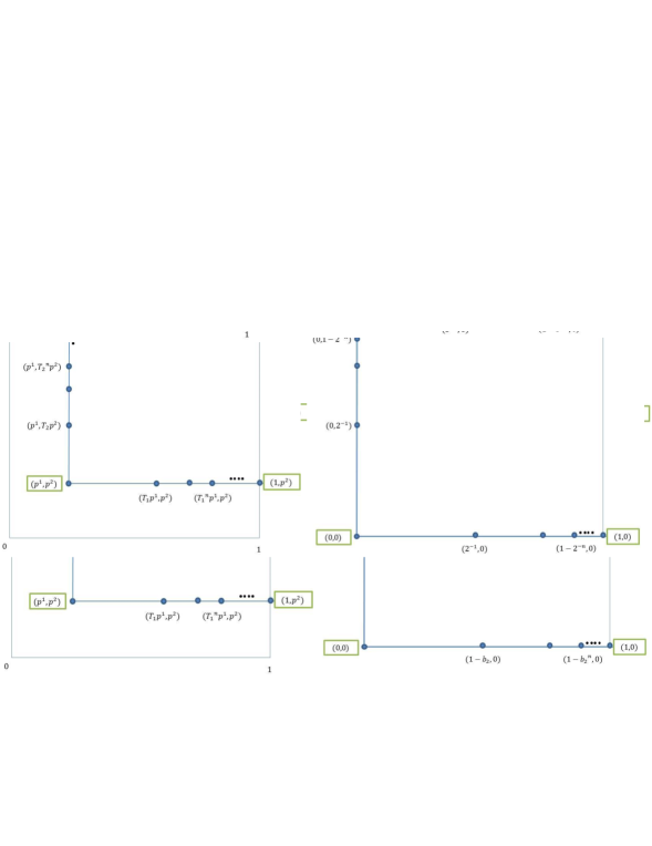
Figure 1: It shows the reachable set $\mathcal{R}$ and the countable state space $\mathcal{S}$.

5.22 Q-learning algorithm for the POMDP

Let $b_{1},b_{2}$ be any arbitrary number in $(0,1)$ and $B:\mathcal{R}\mapsto{\mathbb{Z}^{+}}^{2}$ be a bijective function that maps each state of $\mathscr{R}$ to a point in ${\mathbb{Z}^{+}}^{2}$ as follows:

$$\left(0,1-b_{1}^{n}\right)=B(p^{1},T_{2}^{n}p^{2}),\left(1-b_{2}^{n},0\right)=B(T_{1}^{n}p^{1},p^{2}),n\in\mathds{N}$$

$$\left(0,1\right)=B(p^{1},1),(1,0)=B(1,p^{2}),\left(1,1\right)=B(1,1),(0,0)=B(p^{1},p^{2})$$

where $\lim_{n\rightarrow\infty}B(p^{1},T_{2}^{n}p^{2})=B(p^{1},1)$ and $\lim_{n\rightarrow\infty}B(T_{1}^{n}p^{1},p^{2})=B(1,p^{2})$. Define a countable-state MDP $\Delta$ with state space $\mathcal{S}$, action space $\mathcal{A}$, dynamics $\tilde{f}$, and cost function $\tilde{\ell}$ as follows:

(F1) Let $\mathcal{S}=\{S_{k}\}_{k=1}^{\infty}$ be the state space, where $S_{1}=\{(0,0)\}$ and $S_{k}=\{(0,0),(0,1),(1,0),(1,1),(0,1-b_{1}^{i}),(1-b_{2}^{i},0)\}_{i=1}^{k-1}$, $k\geq 2$. The action space is $\mathcal{A}=\{(0,1),(1,0),(1,1)\}$. The initial state $S_{1}=(0,0)$. The state $S_{t}\in\mathcal{S}_{k}$, $k\leq t$, evolves as follows: for $\mathbf{A}_{t}\in\mathcal{A},\mathbf{U}_{t}\in\{0,1\}^{2}$,

$$S_{t+1}=\tilde{f}(S_{t},\mathbf{A}_{t},\mathbf{U}_{t}),\quad S_{t+1}\in\mathcal{S}_{k+1}.$$ (34)

For ease of exposition of dynamics $\tilde{f}$, we denote every state $S_{t}\in\mathcal{S}_{k}$ in a format of $(1-b_{2}^{k_{2}},1-b_{1}^{k_{1}})$, where $k_{1},k_{2}$ take value in the set of $\{0,1,\ldots,\infty\}$. Thus,

$$\tilde{f}(S_{t},\mathbf{A}_{t},\mathbf{U}_{t})=\begin{cases}(0,1-b_{1}^{(k_{1}+1)})&\mathbf{A}_{t}=(1,0)\\ (1-b_{2}^{(k_{2}+1)},0)&\mathbf{A}_{t}=(0,1)\\ (1,1)&\mathbf{A}_{t}=(1,1),\mathbf{U}_{t}=(1,1)\\ (0,0)&\mathbf{A}_{t}=(1,1),\mathbf{U}_{t}\neq(1,1)\end{cases}$$

At time $t$, there is a cost given by

$$\tilde{\ell}(S_{t},\mathbf{A}_{t})=\hat{\ell}(B^{-1}(S_{t}),\mathbf{A}_{t}).$$ (35)

It is trivial to see that the tuple $\langle\{\mathcal{S}_{k}\}_{k=1}^{\infty},B^{-1},\tilde{f}\rangle$ is an IER because of the fact that

$$\phi(\cdot,\mathbf{a},\mathbf{u})=B^{-1}\left(\tilde{f}\left(B(\cdot),\mathbf{a},\mathbf{u})\right)\right),\quad\forall\mathbf{a}\in\mathcal{A},\mathbf{u}\in\{0,1\}^{2}.$$

(F2) State space $\mathcal{S}$, action space $\mathcal{A}$, and dynamics $\tilde{f}$ do not depend on the unknowns i.e. $(p^{1},p^{2},\ell^{1},\ell^{2},\ell^{3})$.

The performance of a stationary strategy $\tilde{\bm{\psi}}:\mathcal{S}\mapsto\mathcal{A}$ is quantified by (16). According to Lemma 2, we can restrict attention in solving MDP $\Delta$ instead of the POMDP without loss of optimality. Let $\Delta_{N}$ be a finite-state MDP with state space $\mathcal{S}_{N}$ and action space $\mathcal{A}$. The initial state $S_{1}=(0,0)$. At time $t$, state $S_{t}\in\mathcal{S}_{N}$ evolves as follows: for any $\mathbf{A}_{t}\in\mathcal{A},\mathbf{U}_{t}\in\{0,1\}^{2}$,

$$S_{t+1}=\begin{dcases}\tilde{f}(S_{t},\mathbf{A}_{t},\mathbf{U}_{t})&\tilde{f}(S_{t},\mathbf{A}_{t},\mathbf{U}_{t})\in\mathcal{S}_{N}\\ (1-b_{2},0)&\tilde{f}(S_{t},\mathbf{A}_{t},\mathbf{U}_{t})\in\mathcal{S}_{N+1}\backslash\mathcal{S}_{N}\end{dcases}$$ (36)

In (36), whenever state $s_{t}$ steps out of $S_{N}$, the users take a sequence of actions as follows: At first, user 1 transmits and user 2 does not transmit, then user 2 transmits and user 1 does not transmit. This sequence of actions takes the system to state $(1-b_{2},0)\in S_{N},N\geq 2$. Now, we use standard Q-learning algorithm as the generic RL algorithm $\mathcal{T}$ to learn the optimal strategy of $\Delta_{N}$.

Algorithm 2    Decentralized Q-learning Algorithm

1:Given $\epsilon>0$, choose a sufficiently large $N\in\mathbb{N}$ such that $\frac{2\beta^{N}}{1-\beta}L\leq\epsilon$. Then, construct state space $\mathcal{S}_{N}$, action space $\mathcal{A}$, and dynamics $\tilde{f}$. Let $s_{1}=(0,0)$. Initialize Q-functions with zero and step-sizes $\alpha$ with one i.e $Q(s,\mathbf{a})=0,\alpha(s,\mathbf{a})=1,\forall s\in\mathcal{S}_{N},\forall\mathbf{a}\in\mathcal{A}$.

2:At iteration $k\in\mathbb{N}$, users uniformly pick a random action $\ \mathbf{a}_{k}\in\mathcal{A}$ at state $s_{k}\in\mathcal{S}_{N}$ by means of a common shared random number generator. Then, user $i\in\{1,2\}$ takes action $u^{i}_{k}$ according to the chosen $a^{i}_{k}$ and local information $x^{i}_{k}\in\{0,1\}$ as follows:

$$u^{i}_{k}=a^{i}_{k}\cdot x_{k}^{i}.\quad i=1,2.\vspace{-.1cm}$$

3:Based on the taken actions, the system incurs a cost $\ell_{k}$ and generates $(x^{1}_{k+1},x^{2}_{k+1},\mathbf{u}_{k}=(u^{1}_{k},u^{2}_{k}))$. Since $\mathbf{u}_{k}$ is observable to both users, they consistently compute the next state

$$s_{k+1}=\tilde{f}(s_{k},\mathbf{a}_{k},\mathbf{u}_{k}).\vspace{-.1cm}$$

If $s_{k+1}\notin\mathcal{S}_{N}$, user 1 transmits first and then, user 2 transmits, and the state of system will be transmitted to $s_{k+1}=(1-b_{2},0)$; otherwise, the system proceeds from $s_{k+1}\in\mathcal{S}_{N}$.

4:Users update the corresponding Q-function associated with the pair $(s_{k},\mathbf{a}_{k})$ as follows:

$$Q(s_{k},\mathbf{a}_{k})\leftarrow(1-\alpha(s_{k},\mathbf{a}_{k}))Q(s_{k},\mathbf{a}_{k})+\alpha(s_{k},\mathbf{a}_{k})\left(\ell_{k}+\beta\min_{v\in\mathcal{A}}Q(s_{k+1},v)\right)\vspace{-.1cm}$$

Also, the corresponding step-size are updated:

$$\frac{1}{\alpha(s_{k},\mathbf{a}_{k})}\leftarrow\frac{1}{\alpha(s_{k},\mathbf{a}_{k})}+1.$$

5:$k\leftarrow k+1$, and go to step 2 until termination.

6:

According to [3, Theorem 3], Q-functions in Algorithm 2 will converge to a $Q^{\ast}$ with probability one. Let $Q^{\ast}$ be the resultant limit. Then, the optimal strategy $\tilde{\bm{\psi}_{N}^{\ast}}$ is as follows:

$$\tilde{\bm{\psi}_{N}^{\ast}}=\operatornamewithlimits{argmin}_{\mathbf{a}\in\mathcal{A}}(Q^{\ast}(\cdot,\mathbf{a})).$$ (37)

The strategy $\bm{g}^{\ast}_{N}$ is $\epsilon_{N}$-optimal where

$$g^{i,\ast}_{N}(s)(x):=\tilde{\bm{\psi}_{N}^{i,\ast}}(s)\cdot x,\quad\forall s\in\mathcal{S}_{N},x\in\{0,1\},i=1,2$$

where $\tilde{\bm{\psi}_{N}^{i,\ast}}$ denotes $i$th term of $\tilde{\bm{\psi}_{N}^{\ast}}$.

5.23 Numerical Results

In this section, we provide a numerical simulation that shows the strategy learned by decentralized Q-learning Algorithm 2 converges to an optimal strategy when the arrival probabilities are $(p^{1},p^{2})=(0.3,0.6)$ and the cost functions are $\ell^{1}=\ell^{2}=-1,\ell^{3}=0$.

Suppose users have no packets at the beginning. Users wait one time step to receive packets (i.e. user 1 receives a packet with $p^{1}=0.3$ probability and user 2 receives a packet with $p^{2}=0.6$ probability). At $t=1$, action $(0,1)$ is optimal i.e. the user $2$ transmits and user $1$ does not transmit. At $t\geq 2$, state $s_{t}$ enters a recurrent class under the optimal strategy, and stays there forever. The recurrent class includes four states: $(0,1-b_{1}^{1})$, $(1-b_{2}^{1},0)$, $(1-b_{2}^{2},0)$, and $(1-b_{2}^{3},0)$. One immediate result is that for any $N\geq 4$, state $S_{t}$ will never step out of $\mathcal{S}_{N}$ under the optimal strategy which implies $\tau_{N}=\infty$ and hence $\epsilon_{N}$ in Theorem 3 is zero (i.e. optimal strategy). For $t\geq 2$, the optimal strategy is a sequence of the following actions $(0,1),(0,1),(1,0),(0,1)$. Thus, it means that user 2 should transmit $3$ times more than user 1 to minimize the number of collisions (maximize the number of successful transmission). Figure 2 displays a few snapshots of state $s_{t}$ governed by the strategy under the learning procedure where the learned strategy will eventually take state $s_{t}$ to the optimal recurrent class.

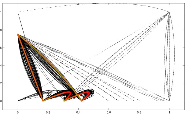
Figure 2: This figure displays the learning procedure of optimal strategy in a few snapshots. It is seen that the state of the system is eventually trapped in the optimal recurrent class. The learning procedure is plotted in black and the optimal recurrent class is plotted in red. In this simulation, we use the following numerical values: $b_{1}=0.25,b_{2}=0.83,N=20,\beta=0.99,p^{1}=0.3,p^{2}=0.6,\ell^{1}=\ell^{2}=-1,\ell^{3}=0.$

6 Conclusion

In this paper, we proposed a novel approach to develop a finite-state RL algorithm, for a large class of decentralized control systems with partial history sharing information structure, that guarantees $\epsilon-$team-optimal solution. We presented our approach in two steps. In the first step, we used the common information approach to obtain an equivalent centralized POMDP of the decentralized control problem. However, the resultant POMDP can not be used directly because it requires the complete knowledge of the model while the agents only know the model incompletely. Thus, in the second step, we introduced a new methodology to develop a RL algorithm for the obtained centralized POMDP. In particular, to remove the dependency of the complete knowledge, we introduced Incrementally Expanding Representation (IER) and based on that, we constructed a finite-state RL algorithm. In addition, we illustrated our approach by developing a decentralized Q-learning algorithm for two-user Multi Access Broadcast Channel (MABC), a benchmark example for decentralized control systems. The numerical simulations verify that the learned strategy converges to an optimal strategy.

References

• [1] S. Yuksel and T. Basar, Stochastic Networked Control Systems, 2013.
• [2] A. Nayyar, A. Mahajan, and D. Teneketzis, Decentralized Stochastic Control with Partial History Sharing: A Common Information Approach, IEEE Trans. on Automatic Control, vol. 58, no. 7, Jul., 2013.
• [3] J. N. Tsitsiklis, Synchronous Stochastic Approximation and Q-Learning, Machine Learning, vol. 16, pp. 185-202, 1994.
• [4] M. G. Hluchyj and R. G. Gallager, Multiacces of a slotted channel by finitely many users, Proc. of Nat. Tel. Con., pp. 421-427, 1981.
• [5] J. M. Ooi and G. W. Wornell, “Decentralized control of a mutliple access broadcast channel: performance bounds,” Proc. of the 35th Conference on Decision and Control, pp. 293-298, 1996.
• [6] A. Mahajan, Optimal transmission policies for two-user multiple access broadcast using dynamic team theory, IEEE 48th Annual Allerton Conf. on, pp. 806–813, Sept., 2010.
• [7] A. Mahajan, A. Nayyar, and D. Teneketzis, “Identifying tractable decentralized control problems on the basis of information structure,” Proc. 46th Annual Allerton Conf., pp. 1440-1449, 2008.
• [8] S. Seuken and S. Zilberstein, “Memory-bounded dynamic programming for DEC-POMDPs,” in Proceedings of the 20th international joint conference on Artificial intelligence, pp. 2009-2015, USA, 2007.
• [9] J. S. Dibangoye, A.-I. Mouaddib, and B. Chaib-draa, Incremental pruning heuristic for solving DEC-POMDPs,” Proc. of Workshop on Multiagent Sequential Decision Making in Uncertain Domains , 2008.
• [10] M. T. J. Spaan, N. Vlassis, and F. C. A. Groen, High level coordination of agents based on multiagent Markov decision processes with roles, in Workshop on Coop. Rob., IEEE/RSJ Int., pp. 66-73, 2002.
• [11] N. Vlassis, A concise introduction to multiagent systems and distributed AI,Univ. of Amsterdam, The Netherlands, Tech. Rep., 2003.
• [12] J. R. Kok, M. T. J. Spaan, and N. Vlassis, Non-communicative multirobot coordination in dynamic environment, Robotics and Autonomous Systems, Vol. 50, No. 2-3, pp. 99-114, 2005.
• [13] C. Claus and C. Boutilier, The dynamics of reinforcement learning in cooperative multiagent systems, 10th Conf. on Inn. Appl. of AI , pp. 746-752, 1998.
• [14] S. Kapetanakis and D. Kudenko, Reinforcement learning of coordination in cooperative multi-agent systems, 14th conf. on Inn. Appl. of AI , pp. 326-331, 2002.
• [15] L. Matignon, G. J. Laurent, and N. Le Fort-Piat, Hysteretic Q-Learning : an algorithm for Decentralized Reinforcement Learning in Cooperative Multiagent Teams,
• [16] J. huang, B. Yang, and D. Y. Liu, A distributed Q-learning Algorithm for Multi-Agent Team coordination, IEEE 40th Int. conf. on Mach. Ler. and Cyb., Vol. 1, pp. 108-113, Aug., 2005.
• [17] A. Nayyar, A. Mahajan, and D. Teneketzis, Optimal control strategies in delayed sharing information structures, IEEE Tran. on Automatic Control, vol. 56, no. 7, pp. 1606-1620, Jul., 2011.
• [18] J. M Ooi, Sh. M. Verbout, J. T. Ludwig, and G. W. Wornell, A separation theorem for periodic sharing information patterns in decentralized control, IEEE transactions on Automatic Control, vol. 42, no. 11, pp. 1546–1550, 1997.
• [19] J. Arabneydi and A. Mahajan, Team optimal control of coupled subsystems with mean-field sharing, IEEE, Conference on decision and Control, Dec., 2014.
• [20] A. Mahajan, Optimal Decentralized Control of Coupled agents with Control Sharing, IEEE Transaction on Automatic Control, vol. 58, no. 9, Sept., 2013.
• [21] R. Murphey and P. Pardalos, Cooperative control and optimization, Springer Science & Business Media, vol. 66, 2002.
• [22] K. Pivazyan and Y. Shoham, Polynomial-time reinforcement learning of near-optimal policies, AAAI/IAAI, pp 205–210, 2002.
• [23] E. Even-Dar, Algorithms for Reinforcement Learning, Ph.D. thesis, TAV university, 2005.