Neural Prototype Trees for Interpretable Fine-grained Image Recognition

Abstract

Prototype-based methods use interpretable representations to address the black-box nature of deep learning models, in contrast to post-hoc explanation methods that only approximate such models. We propose the Neural Prototype Tree (ProtoTree), an intrinsically interpretable deep learning method for fine-grained image recognition. ProtoTree combines prototype learning with decision trees, and thus results in a globally interpretable model by design. Additionally, ProtoTree can locally explain a single prediction by outlining a decision path through the tree. Each node in our binary tree contains a trainable prototypical part. The presence or absence of this learned prototype in an image determines the routing through a node. Decision making is therefore similar to human reasoning: Does the bird have a red throat? And an elongated beak? Then it’s a hummingbird! We tune the accuracy-interpretability trade-off using ensemble methods, pruning and binarizing. We apply pruning without sacrificing accuracy, resulting in a small tree with only 8 learned prototypes along a path to classify a bird from 200 species. An ensemble of 5 ProtoTrees achieves competitive accuracy on the CUB-200- 2011 and Stanford Cars data sets. Code is available at github.com/M-Nauta/ProtoTree.

1 Introduction

There is an ongoing scientific dispute between simple, interpretable models and complex black boxes, such as Deep Neural Networks (DNNs). DNNs have achieved superior performance, especially in computer vision, but their complex architectures and high-dimensional feature spaces has led to an increasing demand for transparency, interpretability and explainability [1], particularly in domains with high-stakes decisions [43]. In contrast, decision trees are easy to understand and interpret [14, 19], because they transparently arrange decision rules in a hierarchical structure. Their predictive performance is however far from competitive for computer vision tasks. We address this so-called ‘accuracy-interpretability trade-off’ [1, 35] by combining the expressiveness of deep learning with the interpretability of decision trees.

We present the Neural Prototype Tree, ProtoTree in short, an intrinsically interpretable method for fine-grained image recognition. A ProtoTree has the representational power of a neural network, and contains a built-in binary decision tree structure, as shown in Fig. 1 (left). Each internal node in the tree contains a trainable prototype. Our prototypes are prototypical parts learned with backpropagation, as introduced in the Prototypical Part Network (ProtoPNet) [9] where a prototype is a trainable tensor that can be visualized as a patch of a training sample. The extent to which this prototype is present in an input image determines the routing of the image through the corresponding node. Leaves of the ProtoTree learn class distributions. The paths from root to leaves represent the learned classification rules. The reasoning of our model is thus similar to the “Guess Who?” game where a player asks a series of binary questions related to visual properties to find out which of the 24 displayed images the other player had in mind.

To this end, a ProtoTree consists of a Convolutional Neural Network (CNN) followed by a binary tree structure and can be trained end-to-end with a standard cross-entropy loss function. We only require class labels and do not need any other annotations. To make the tree differentiable and back-propagation compatible, we utilize a soft decision tree, meaning that a sample is routed through both children, each with a certain weight. We present a novel routing procedure based on the similarity between the latent image embedding and a prototype. We show that a trained soft ProtoTree can be converted to a hard, and therefore more interpretable, ProtoTree without loss of accuracy.

A ProtoTree approximates the accuracy of non-interpretable classifiers, while being interpretable-by-design and offering truthful global and local explanations. This way it provides a novel take on interpretable machine learning. In contrast to post-hoc explanations, which approximate a trained model or its output [37, 31], a ProtoTree is inherently interpretable since it directly incorporates interpretability in the structure of the predictive model [37]. A ProtoTree therefore faithfully shows its entire classification behaviour, independent of its input, providing a global explanation (Fig. 1). As a consequence, our compact tree enables a human to convey, or even print out, the whole model. In contrast to local explanations, which explain a single prediction and can be unstable and contradicting [3, 27], global explanations enable simulatability [35]. Additionally, our ProtoTree can produce local explanations by showing the routing of a specific input image through the tree (Fig. 1, right). Hence, ProtoTree allows retraceable decisions in a human-comprehensible number of steps. In case of a misclassification, the responsible node can be easily identified by tracking down the series of decisions, which eases error analysis.

Scientific Contributions

• An intrinsically interpretable neural prototype tree architecture for fine-grained image recognition.

• Outperforming ProtoPNet [9] while having roughly only 10% of the number of prototypes, included in a built-in hierarchical structure.

• An ensemble of 5 interpretable ProtoTrees achieves competitive performance on CUB-200-2011 [50] (CUB) and Stanford Cars [30].

2 Related Work

Within computer vision, various explainability strategies exist for different notions of interpretability. A machine learning model can be explained for a single prediction, part-based methods [56, 61], saliency maps [6, 13, 60] or representer points [53]. Others explain the internals of a model, with activation maximization [39, 41] to visualize neurons, deconvolution or upconvolution [12, 54] to explain layers, generating image exemplars [18] to explain the latent space, or concept activation vectors [26] to explain model sensitivity. While such post-hoc methods give an intuition about the black-box model, intrinsic interpretable models such as classical decision trees, are fully simulatable since they faithfully show the decision making process. Similarly, by utilizing interpretable features as splitting criteria, a ProtoTree’s decision making process can be understood in its entirety, as well as for a single prediction. ProtoTree combines prototypical feature representations (Sec. 2.1) with soft-decision tree learning (Sec. 2.2).

2.1 Interpretability with Prototypes

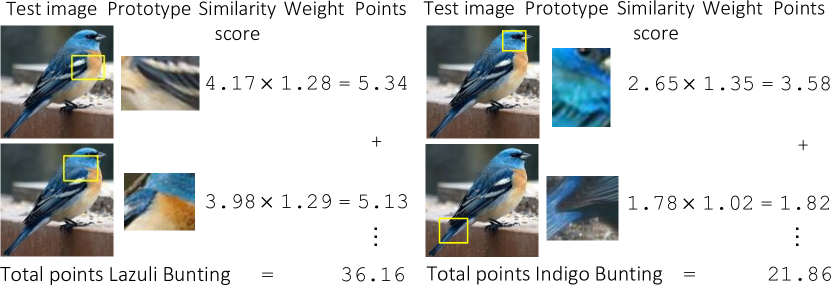
Figure 2: Excerpt from classification process of ProtoPNet [9]. ProtoPNet learns 10 prototypes per class, resulting in 2000 prototypes for CUB, therefore making 2000 local decisions for one test image.

Prototypes are visual explanations that can be incorporated in a model for intrinsic interpretability. ProtoAttend [5] and DMR [4] use full images. In contrast, we go for prototypical parts to break up the decision making process in small steps. Our choice is supported by BagNet [8] which found that “even complex perceptual tasks like ImageNet can be solved just based on small image features and without any notion of spatial relationships”. Related is the Classification-By-Components network [44] that learns positive, negative and indefinite visual components motivated by the recognition-by-components theory [7] describing how humans recognize objects by segmenting it into multiple components.

We build upon the Prototypical Part Network (ProtoPNet) [9], an intrinsically interpretable deep network architecture for case-based reasoning. Since their prototypes have smaller spatial dimensions than the image itself, they represent prototypical parts and are therefore suited for fine-grained image classification. ProtoPNet learns a pre-determined number of prototypical parts (prototypes) per class. To classify an image, the similarity between a prototype and a patch in the image is calculated by measuring the distance in latent space. The resulting similarity scores are weighted by values learned by a fully-connected layer. The explanation of ProtoPNet shows the reasoning process for a single image, by visualizing all prototypes together with their weighted similarity score. Summing the weighted similarity scores per class gives a final score for the image belonging to each class, as shown in Fig. 2. We improve upon ProtoPNet by showing an easy-to-interpret global explanation by means of a decision tree. Such a hierarchical, logical model aids interpretability [14, 43], since a tree has various conceptual advantages compared to a linear bag-of-prototypes: a tree enforces a sequence of steps and it supports negative associations (absence of prototype), thereby reducing the number of prototypes and better mimicking human reasoning. The hierarchical structure therefore enhances interpretability and could also lead to more insights w.r.t. clusters in the data. Instead of multiplying similarity scores with weights, our local explanation shows the routing of a sample through the tree. Furthermore, we do not have class-specific prototypes, do not need to learn weights for similarity scores and we use a simple cross-entropy loss function.

2.2 Neural Soft Decision Trees

(a) DNDF [33]

(b) SDT [15]

(c) SDT [22]

(d) Ours

Figure 3: Visualized root node from soft decision trees. Applied to resp. CIFAR10, MNIST, FashionMNIST and CUB. Republished with permission from the authors (a-c).

Soft Decision Trees (SDTs) have shown to be more accurate than traditional hard decision trees [23, 24, 46]. Only recently deep neural networks are integrated in binary SDTs. The Deep Neural Decision Forest (DNDF) [29] is an ensemble of neural SDTs: a neural network learns a latent representation of the input, and each node learns a routing function. Adaptive Neural Trees [47] (ANTs) are a generalization of DNDF. Each node can transform and route its input with a small neural network. In contrast to most SDTs that require a fixed tree structure, including ours, ANTs greedily learn a binary tree topology. Such greedy algorithms however could lead to suboptimal trees [40], and are only applied to simple classification problems such as MNIST. Furthermore, the above methods lose the main attractive property of decision trees: interpretability. DNDFs can be locally interpreted by visualizing a path of saliency maps [33], as shown in Fig. 3(a). Frosst & Hinton [15] train a perceptron for each node, and visualize the learned weights (Fig. 3(b)). The limited representational power of perceptrons however leads to suboptimal classification results. The approach in [22] makes SDTs deterministic at test time and linear split parameters can be visualized and enhanced with a spatial regularization term (Fig. 3(c)). In contrast to these interpretable methods, we apply our method to natural images for fine-grained image recognition and our visualizations are sharp and full-color, therefore improving interpretability (Fig. 3(d)). Instead of image recognition, Neural-Backed Decision Trees for Segmentation [52] use visual decision rules with saliency maps for segmentation.

Other tree approaches for image classification acpply post-hoc explanation techniques, by showing example images per node [2, 55], visualizing typical CNN filters of each node that can be manually labelled [55], showing class activation maps [25] or manual inspection of leaf labels and the meaning of internal nodes [51]. We extend prior work by including prototypes in a tree structure, thereby obtaining a globally explainable, intrinsically interpretable model with only one decision per node. Additionally, similar to ProtoPNet [9], a ProtoTree does not require manual labelling and is therefore self-explanatory. Our work differs from hierarchical image classification (, a gibbon is an animal and a primate) such as [20], since we do not require hierarchical labels or a predefined taxonomy.

3 Neural Prototype Tree

A Neural Prototype Tree (ProtoTree) hierarchically routes an image through a binary tree for interpretable image recognition. We now formalise the definition of a ProtoTree for supervised learning. Consider a classification problem with training set $\bm{\mathcal{T}}$ containing $N$ labelled images $\{(\bm{x}^{(1)},y^{(1)}),...,(\bm{x}^{(N)},y^{(N)})\}\in\mathcal{X}\times\mathcal{Y}$. Given an input image $\bm{x}$, a ProtoTree predicts the class probability distribution over $K$ classes, denoted as $\hat{\bm{y}}$. We use $\bm{y}$ to denote the one-hot encoded ground-truth label $y$ such that we can train a ProtoTree by minimizing the cross-entropy loss between $\bm{y}$ and $\hat{\bm{y}}$. A ProtoTree can also be trained with soft labels from a trained model for knowledge distillation, similar to [15].

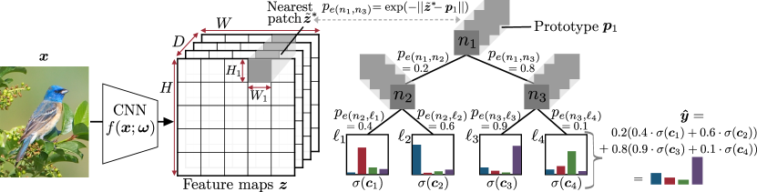
Figure 4: Decision making process of a ProtoTree to predict class probability distribution $\bm{\hat{y}}$ of input image $\bm{x}$. During training, prototypes $\bm{p}_{n}\in\bm{P}$, leaves’ class distributions $\bm{c}$ and CNN parameters $\omega$ are learned. Probabilities $p_{e}$ (shown with example values) depend on the similarity between a patch in the latent input image and a prototype.

A ProtoTree $T$ is a combination of a convolutional neural network (CNN) $f$ with a soft neural binary decision tree structure. As shown in Fig. 4, an input image is first forwarded through $f$. The resulting convolutional output $\bm{z}=f(\bm{x};\bm{\omega})$ consists of $D$ two-dimensional ($H\times W$) feature maps, where $\bm{\omega}$ denotes the trainable parameters of $f$. Secondly, the latent representation $\bm{z}\in\mathbb{R}^{H\times W\times D}$ serves as input for a binary tree. This tree consists of a set of internal nodes $\mathcal{N}$, a set of leaf nodes $\mathcal{L}$, and a set of edges $\mathcal{E}$. Each internal node $n\in\mathcal{N}$ has exactly two child nodes: $n.\mathit{left}$ connected by edge $e(n,n.\mathit{left})\in\mathcal{E}$ and $n.\mathit{right}$ connected by $e(n,n.\mathit{right})\in\mathcal{E}$. Each internal node $n\in\mathcal{N}$ corresponds to a trainable prototype $\bm{p}_{n}\in\bm{P}$. We follow the prototype definition of ProtoPNet [9] where each prototype is a trainable tensor of shape $H_{1}\times W_{1}\times D$ (with $H_{1}\leq H$, $W_{1}\leq W$, and in our implementation $H_{1}=W_{1}=1$) such that the prototype’s depth corresponds to the depth of the convolutional output $\bm{z}$.

We use a form of generalized convolution without bias [17], where each prototype $\bm{p}_{n}\in\bm{P}$ acts as a kernel by ‘sliding’ over $\bm{z}$ of shape $H\times W\times D$ and computes the Euclidean distance between $\bm{p}_{n}$ and its current receptive field $\tilde{\bm{z}}$ (called a patch). We apply a minimum pooling operation to select the patch in $\bm{z}$ of shape $H_{1}\times W_{1}\times D$ that is closest to prototype $\bm{p}_{n}$:

$$\tilde{\bm{z}}^{*}=\mathop{\mathrm{argmin}}_{\tilde{\bm{z}}\in\mathit{patches}(\bm{z})}||\tilde{\bm{z}}-\bm{p}_{n}||.$$ (1)

The distance between the nearest latent patch $\tilde{\bm{z}}^{*}$ and prototype $\bm{p}_{n}$ determines to what extent the prototype is present anywhere in the input image, which influences the routing of $\bm{z}$ through corresponding node $n$. In contrast to traditional decision trees, where an internal node routes sample $\bm{z}$ either right or left, our node $n\in\mathcal{N}$ is soft and routes $\bm{z}$ to both children, each with a fuzzy weight within $[0,1]$, giving it a probabilistic interpretation [15, 23, 29, 47]. Following this probabilistic terminology, we define the similarity between $\tilde{\bm{z}}^{*}$ and $\bm{p}_{n}$, and therefore the probability of routing sample $\bm{z}$ through the right edge as

$$p_{e(n,n.\mathit{right})}(\bm{z})=\exp(-||\tilde{\bm{z}}^{*}-\bm{p}_{n}||),$$ (2)

such that $p_{e(n,n.\mathit{left})}=1-p_{e(n,n.\mathit{right})}$. Thus, the similarity between prototype $\bm{p}_{n}$ and the nearest patch in the convolutional output, $\tilde{\bm{z}}^{*}$, determines to what extent $\bm{z}$ is routed to the right child of node $n$. Because of the soft routing, $\bm{z}$ is traversed through all edges and ends up in each leaf node $\ell\in\mathcal{L}$ with a certain probability. Path $\mathcal{P}_{\ell}$ denotes the sequence of edges from the root node to leaf $\ell$. The probability of sample $\bm{z}$ arriving in leaf $\ell$, denoted as $\bm{\pi}_{\ell}$, is the product of probabilities of the edges in path $\mathcal{P}_{\ell}$:

$$\bm{\pi}_{\ell}(\bm{z})=\prod_{e\in\mathcal{P}_{\ell}}p_{e}(\bm{z}).$$ (3)

Each leaf node $\ell\in\mathcal{L}$ carries a trainable parameter $\bm{c}_{\ell}$, denoting the distribution in that leaf over the $K$ classes that needs to be learned. The softmax function $\sigma(\bm{c}_{\ell})$ normalizes $\bm{c}_{\ell}$ to get the class probability distribution of leaf $\ell$. To obtain the final predicted class probability distribution $\bm{\hat{y}}$ for input image $\bm{x}$, latent representation $\bm{z}=f(\bm{x}|\bm{\omega})$ is traversed through all edges in $T$ such that all leaves contribute to the final prediction $\bm{\hat{y}}$. An example prediction is shown on the right of Fig. 4. The contribution of leaf $\ell$ is weighted by path probability $\bm{\pi}_{\ell}$, such that:

$$\bm{\hat{y}}(\bm{x})=\sum_{\ell\in\mathcal{L}}\sigma(\bm{c}_{\ell})\cdot\bm{\pi}_{\ell}(f(\bm{x};\bm{\omega})).$$ (4)

4 Training a ProtoTree

Training a ProtoTree requires to learn the parameters $\bm{\omega}$ of CNN $f$ for informative feature maps, the nodes’ prototypes $\bm{P}$ for routing and the leaves’ class distribution logits $\bm{c}$ for prediction. The number of prototypes to be learned, $|\bm{P}|$, depends on the tree size. A binary tree structure is initialized by defining a maximum height $h$, which creates $2^{h}$ leaves and $2^{h}-1$ prototypes. Thus, the computational complexity of learning $\bm{P}$ is growing exponentially with $h$.

We require a pre-trained CNN $f$ (on ImageNet or training it on a specific prediction task first). During training, prototypes in $\bm{P}$ are trainable tensors. Parameters $\bm{\omega}$ and $\bm{P}$ are simultaneously learned with back-propagation by minimizing the cross-entropy loss between the predicted class probability distribution $\bm{\hat{y}}$ and ground-truth $\bm{y}$. The learned prototypes should be near a latent patch of a training image such that they can be visualized as an image patch to represent a prototypical part (cf. Sec. 5).

Learning leaves’ distributions. In a classical decision tree, a leaf label is learned from the samples ending up in that leaf. Since we use a soft tree, learning the leaves’ distributions is a global learning problem. Although it is possible to learn $\bm{c}$ with back-propagation together with $\bm{\omega}$ and $\bm{P}$, we found that this gives inferior classification results. We hypothesize that including $\bm{c}$ in the loss term leads to an overly complex optimization problem. Kontschieder et al. [29] noted that solely optimizing leaf parameters is a convex optimization problem and proposed a derivative-free strategy. Translating their approach to our methodology gives the following update scheme for $\bm{c}_{\ell}$ for all $\ell\in\mathcal{L}$:

$$\bm{c}_{\ell}^{(t+1)}=\sum_{\bm{x},\bm{y}\in\bm{\mathcal{T}}}(\sigma(\bm{c}_{\ell}^{(t)})\odot\bm{y}\odot\bm{\pi}_{\ell})\oslash\bm{\hat{y}},$$ (5)

where $t$ indexes a training epoch, $\odot$ denotes element-wise multiplication and $\oslash$ is element-wise division. The result is a vector of size $K$ representing the class distribution in leaf $\ell$. This learning scheme is however computationally expensive: at each epoch, first $\bm{c}_{\ell}^{(t+1)}$ is computed to update the leaves, and then all other parameters are trained by looping through the data again, meaning that $\bm{\hat{y}}$ is computed twice. We propose to do this more efficiently and intertwine mini-batch gradient descent optimization for $\omega$ and $\bm{P}$ with a derivative-free update to learn $\bm{c}$, as shown in Alg. 1. Our algorithm has the advantage that each mini-batch update of $\omega$ and $\bm{P}$ is taken into account for updating $\bm{c}^{(t+1)}$, which aids convergence. Moreover, computing $\bm{\hat{y}}$ only once for each batch roughly halves the training time.

Input: Training set $\bm{\mathcal{T}}$, max height $h$, $nEpochs$

1 initialize ProtoTree $T$ with height $h$ and $\bm{\omega}$, $\bm{P}$, $\bm{c}^{(1)}$;

2 for $t\in\{1,...,nEpochs\}$ do

3       randomly split $\bm{\mathcal{T}}$ into $B$ mini-batches;

4       for $(\bm{x}_{b},\bm{y}_{b})\in\{\bm{\mathcal{T}}_{1},...,\bm{\mathcal{T}}_{b},...,\bm{\mathcal{T}}_{B}\}$ do

5             $\bm{\hat{y}}_{b}=T(\bm{x}_{b})$;

6             compute loss $(\bm{\hat{y}}_{b},\bm{y}_{b})$;

7             update $\omega$ and $\bm{P}$ with gradient descent;

8             for $\ell\in\mathcal{L}$ do

9                   $\bm{c}_{\ell}^{(t+1)}$ -= $\frac{1}{B}\cdot\bm{c}_{\ell}^{(t)}$;

10                   $\bm{c}_{\ell}^{(t+1)}$ += Eq. 5 for $\bm{x}_{b},\bm{y}_{b}$;

11                  

12prune $T$ (optional);

13 replace each prototype $\bm{p}_{n}\in\bm{P}$ with its nearest latent patch $\tilde{\bm{z}}^{*}_{n}$ and visualize;

Algorithm 1 Training a ProtoTree

5 Interpretability and Visualization

To foster global model interpretability, we prune ineffective prototypes, visualize the learned latent prototypes, and convert soft to hard decisions.

5.1 Pruning

Interpretability can be quantified by explanation size [11, 45]. In a ProtoTree $T$, explanation size is related to the number of prototypes. To reduce explanation size, we analyse the learned class probability distributions in the leaves and remove leaves with nearly uniform distributions, little discriminative power. Specifically, we define a threshold $\tau$ and prune all leaves where $\max(\sigma(\bm{c}_{\ell}))\leq\tau$, with $\tau$ being slightly greater than $1/K$ where $K$ is the number of classes. If all leaves in a full subtree $T^{\prime}\subset T$ are pruned, $T^{\prime}$ (and its prototypes) can be removed. As visualized in Fig. 5, ProtoTree $T$ can be reorganized by additionally removing the now superfluous parent of the root of $T^{\prime}$.

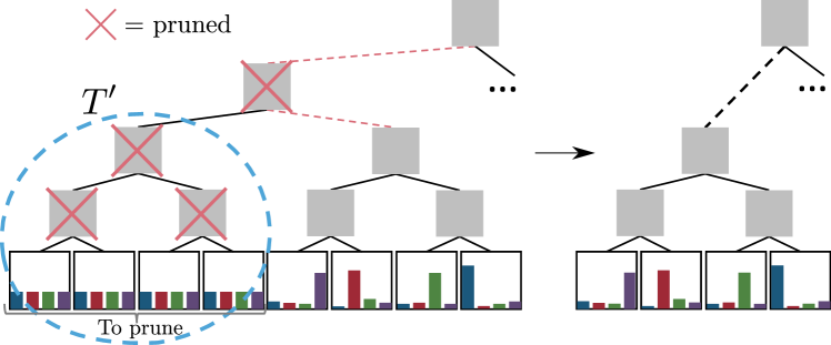
Figure 5: Pruning removes a subtree $T^{\prime}$, and its parent, in which all leaves have an (nearly) uniform distribution.

5.2 Prototype Visualization

Learned latent prototypes need to be mapped to pixel space to enable interpretability. Similar to ProtoPNet [9], we replace each prototype $\bm{p}_{n}\in\bm{P}$ with its nearest latent patch present in the training data, $\tilde{\bm{z}}^{*}_{n}$. Thus,

$$\bm{p}_{n}\leftarrow\tilde{\bm{z}}^{*}_{n},\quad\tilde{\bm{z}}^{*}_{n}=\mathop{\mathrm{argmin}}_{\bm{z}\in\{f(\bm{x}),\forall\bm{x}\in\bm{\mathcal{T}}\}}||\tilde{\bm{z}}^{*}-\bm{p}_{n}||$$ (6)

such that prototype $\bm{p}_{n}$ is equal to latent representation $\tilde{\bm{z}}^{*}_{n}$. Where ProtoPNet replaces its prototypes during training every $10^{th}$ epoch, prototype replacement after training is sufficient for a ProtoTree, since our routing mechanism implicitly optimizes prototypes to represent a certain patch. This reduces computational complexity and simplifies the training process.

We denote by $\bm{x}^{*}_{n}$ the training image corresponding to nearest patch $\tilde{\bm{z}}^{*}_{n}$. Prototype $\bm{p}_{n}$ can now be visualized as a patch of $\bm{x}^{*}_{n}$. We forward $\bm{x}^{*}_{n}$ through $f$ to create a 2-dimensional similarity map that includes the similarity score between $\bm{p}_{n}$ and all patches in $\bm{z}=f(\bm{x}^{*}_{n})$

$$S_{n}^{(i,j)}=\exp(-||\tilde{\bm{z}}^{(i,j)}-\bm{p}_{n}||),$$ (7)

where $(i,j)$ indicates the location of patch $\tilde{\bm{z}}$ in $\mathit{patches}(\bm{z})$. Similarity map $S_{n}$ is upsampled with bicubic interpolation to the input shape of $\bm{x}^{*}_{n}$, after which $\bm{p}_{n}$ is visualized as a rectangular patch of $\bm{x}^{*}_{n}$, at the same location of nearest latent patch $\tilde{\bm{z}}^{*}_{n}$ (see Fig. 6). Thus, instead of merely showing the nearest training patch in the tree, we use the corresponding latent patch $\tilde{\bm{z}}^{*}_{n}$ for routing, making the visualized ProtoTree a faithful model explanation.

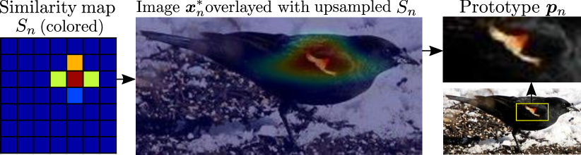
Figure 6: Visualizing a prototype by selecting the most similar patch from the upsampled similarity map.

5.3 Deterministic reasoning

In a soft decision tree, all nodes contribute to a prediction. In contrast, in a hard, deterministic tree, only the nodes along a path account for the final prediction, making hard decision trees easier to interpret than soft trees [2]. Whereas a ProtoTree is soft during training, we propose two possible strategies to convert a ProtoTree to a hard tree at test time:

1. select the path to the leaf with the highest path probability: $\mathop{\mathrm{argmax}}_{\ell\in\mathcal{L}}(\bm{\pi}_{\ell})$

2. greedily traverse the tree, go right at internal node $n$ if $p_{e(n,n.\mathit{right})}>0.5$ and left otherwise.

Sec. 6.2 evaluates to what extent these deterministic strategies influence accuracy compared to soft reasoning.

6 Experiments

We evaluate the accuracy-interpretability trade-off of a ProtoTree, and compare our ProtoTrees with ProtoPNet [9] and state-of-the-art models in terms of accuracy and interpretability. We evaluate on CUB-200-2011 [50] with 200 bird species (CUB) and Stanford Cars [30] with 196 car types (CARS), since both were used by ProtoPNet [9].

6.1 Experimental Setup

We implemented ProtoTree in PyTorch. Our CNN $f$ contains the convolutional layers of ResNet50 [21], pretrained on ImageNet [10] for CARS. For CUB, ResNet50 is pretrained on iNaturalist2017 [49], containing plants and animals and therefore a suitable source domain [32], using the backbone of [59]. Backbone $f$ is frozen for 30 epochs after which $f$ is optimized jointly with the prototypes with Adam [28]. For a fair comparison with ProtoPNet [9], we resize all images to $224\times 224$ such that the resulting feature maps are $7\times 7$. The CNN architecture is extended with a $1\times 1$ convolutional layer to reduce the dimensionality of latent output $\bm{z}$ to $D$, the prototype depth. Based on cross-validation from $\{128,256,512\}$, we used $D$=256 for CUB and $D$=128 for CARS. Similar to ProtoPNet, $H_{1}$=$W_{1}$=$1$ to provide well-sized patches, such that a prototype is of size $1\times 1\times 256$ for CUB. We use ReLU as activation function, except for the last layer which has a Sigmoid function to act as a form of normalization. We initialize the prototypes by sampling from $\mathcal{N}(0.5,0.1)$. The initial leaf distributions $\sigma(\bm{c}_{\ell}^{(1)})$ are uniformly distributed by initializing $\bm{c}_{\ell}^{(1)}$ with zeros for all $\ell\in\mathcal{L}$. See Suppl. for all details.

6.2 Accuracy and Interpretability

Data set	Method           Inter-                       pret.		Top-1 Accuracy	#Proto types
CUB ($224\times 224$)	Triplet Model [34]	-	87.5	n.a.
	TranSlider [58]	-	$85.8$	n.a.
	TASN [57]	o	$87.0$	n.a.
	ProtoPNet [9]	+	$79.2$	$2000$
	ProtoTree $h$=9 (ours)	++	$82.2$$\pm 0.7$	$\bm{202}$
	ProtoPNet ens. (3) [9]	+	$84.8$	$6000$
	ProtoTree ens. (3)	+	$86.6$	$605$
	ProtoTree ens. (5)	+	$\bm{87.2}$	$1008$
CARS ($224\times 224$)	RAU [36]	-	93.8	n.a.
	Triplet Model [34]	-	$93.6$	n.a.
	TASN [57]	o	$93.8$	n.a.
	ProtoPNet [9]	+	$86.1$	$1960$
	ProtoTree $h$=11 (ours)	++	$86.6$$\pm 0.2$	$\bm{195}$
	ProtoPNet ens. (3) [9]	+	$91.4$	$5880$
	ProtoTree ens. (3)	+	$90.3$	$586$
	ProtoTree ens. (5)	+	$\bm{91.5}$	$977$

Table 1: Mean accuracy and standard deviation of our ProtoTree (5 runs) and ensemble with 3 or 5 ProtoTrees compared with self-reported accuracy of uninterpretable state-of-the-art (-), attention-based models (o) and interpretable ProtoPNet (+, with ResNet34-backbone).

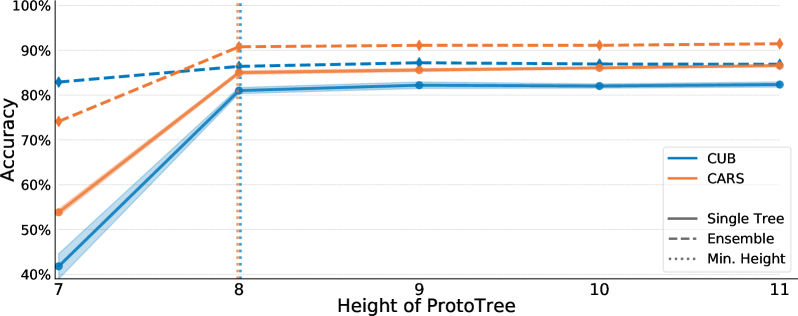
Figure 7: Top-1 accuracy of a ProtoTree (across 5 runs), and an ensemble with those 5 ProtoTrees. A vertical dotted line shows the minimal height such that #leaves $\geq$ #classes.

Table 3 compares the accuracy of ProtoTrees with state-of-the-art methods. Our ProtoTree outperforms ProtoPNet for both datasets. We also evaluated the accuracy of ProtoTree ensembles by averaging the predictions of 3 or 5 individual ProtoTrees, all trained on the same dataset. An ensemble of ProtoTrees outperforms a ProtoPNet ensemble, and approximates the accuracy of uninterpretable or attention-based methods, while providing intrinsically interpretable global and faithful local explanations.

Dataset	$K$	$h$	Initial Acc	Acc pruned	Acc pruned+repl.	# Prototypes	% Pruned	Distance $\tilde{\bm{z}}^{*}_{n}$
CUB	200	9	$82.206\pm 0.723$	$82.192\pm 0.723$	$82.199\pm 0.726$	$201.6\pm 1.9$	60.5	$0.0020\pm 0.0068$
CARS	196	11	$86.584\pm 0.250$	$86.576\pm 0.245$	$86.576\pm 0.245$	$195.4\pm 0.5$	90.5	$0.0005\pm 0.0016$

Table 2: Impact of pruning and prototype replacement: 1) before pruning and replacement, 2) after pruning, 3) after pruning and replacement, 4) number of prototypes after pruning, 5) fraction of prototypes that is pruned and 6) Euclidean distance from each latent prototype to its nearest latent training patch (after pruning). Showing mean and std dev across 5 runs.

Tree Height. A ProtoTree with fewer prototypes is smaller and hence easier to interpret, but represents a less complex model and might have less predictive power. Fig. 7 shows the accuracy of ProtoTrees with increasing height. It confirms that it is sensible to set the initial height $h$ such that the number of leaves is at least as large as the number of classes $K$. For CUB, accuracy increases up to a certain height ($h=9$) after which accuracy plateaus. An increasing height has a higher impact on the accuracy for CARS, probably because of its lower inter-class part similarity for which a more imbalanced tree, with fewer shared prototypes, is more suitable. Ensembling substantially increases prediction accuracy, although at the cost of explanation size.

Pruning. Since our training algorithm optimizes the leaf distributions to minimize the error between $\bm{\hat{y}}$ and one-hot encoded $\bm{y}$, most leaves learn either one class label, or an almost uniform distribution, as shown in Fig. 8 (top left) for CUB with $h$=8. Other datasets and tree heights show a similar pattern (Suppl.). We set pruning threshold $\tau=0.01$, such that we are left with leaves that can be interpreted (nearly) deterministically. Table 2 shows that the prediction accuracy of a ProtoTree barely changes when the tree is pruned and visualized. The negligible difference after prototype replacement (visualization) is supported by the fact that the distance from each prototype to its nearest patch is close to zero, indicating that ProtoTree already implicitly optimizes prototypes to be near a latent image patch. This confirms that replacing prototypes after training suffices, instead of during training as in ProtoPNet [9]. Furthermore, pruning drastically reduces the size of the tree (up to $>90\%$), preserving roughly 1 prototype per class. In contrast, ProtoPNet [9] uses 10 prototypes per class (cf. Tab. 3), resulting in 2000 prototypes in total for CUB. Thus, a ProtoTree is almost 90% smaller and therefore easier to interpret. Even with an ensemble of ProtoTrees, which increases global explanation size, the number of prototypes is still substantially smaller than ProtoPNet (cf. Table 3).

Deterministic reasoning.

Strategy	Accuracy	Fidelity	Path length
Soft	$82.20\pm 0.01$	n.a.	n.a.
Max $\bm{\pi}_{\ell}$	$82.19\pm 0.01$	$0.999\pm 0.001$	$8.3\pm 1.1$ $(9,3)$
Greedy	$82.07\pm 0.01$	$0.987\pm 0.002$	$8.3\pm 1.1$ $(9,3)$

Table 3: Soft vs. deterministic classification strategies at test time. Fidelity is agreement with soft strategy. Min and max path lengths in brackets. ProtoTree on CUB ($h$=9, pruned and replaced), averaged over 5 runs (mean, stdev).

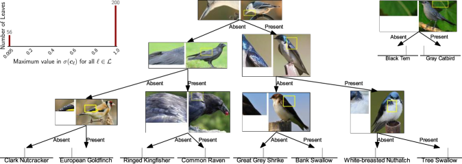
Figure 8: Subtree of an automatically visualized ProtoTree trained on CUB, $h$=8 (middle). Each internal node contains a prototype (left) and the training image from which it is extracted (right). A ProtoTree faithfully shows its reasoning and clusters similar classes (birds with a white chest). Top left: maximum values of all leaf distributions. Top right: ProtoTree reveals biases learned by the model: classifying a Gray Catbird based on the presence of a leaf. Best viewed in color.

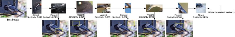
Figure 9: Local explanation that shows the greedy path when classifying a White-breasted Nuthatch. Prototypes found in the test image are: a dark-colored tail, a contrastive eye, sky background (learned bias), a white chest and a blue-grey wing.

As discussed in Sec. 5.3, a ProtoTree can make deterministic predictions at test time to improve human understanding of the decision making process. Table 3 shows that selecting the leaf with the highest path probability leads to nearly the same prediction accuracy as soft routing, since the fidelity (fraction of test images for which the soft and hard strategy make the same classification [19]) is practically 1. The greedy strategy performs slightly worse but its fidelity is still close to 1. Results are similar for other datasets and tree heights (Suppl.). Our experiments therefore show that a ProtoTree can be safely converted to a deterministic tree, such that a prediction can be explained by presenting one path in the tree. Compared to ProtoPNet [9], where a user is required to analyse 2000 prototypes to understand a single prediction for CUB, our deterministic ProtoTree ($h$=9) reduces the number of decisions to follow to 9 prototypes at maximum. When using a more accurate ensemble of 5 deterministic ProtoTrees, a maximum of only 45 prototypes needs to be analysed, resulting in much smaller local explanations than ProtoPNet.

Visualizations and Discussion. Figure 8 shows a snippet of a ProtoTree trained on CUB (more in Suppl.), and Figure 9 shows a local explanation containing the full path along the tree with a greedy classification strategy. From analysing various ProtoTrees, we conclude that prototypes are in general perceptually relevant, and successfully cluster similar-looking classes. Similar to ProtoPNet [9], some prototypes seem to focus on background. This is not necessarily an error in our visualization but shows that a ProtoTree can reveal learned biases. For example, Fig. 8 (top right) shows a green leaf to distinguish between a Gray Catbird and a Black Tern, because the latter is in the training data usually surrounded by sky or water. Further research could investigate to what extent undesired prototypes can be ‘fixed’ with a human-in-the-loop that replaces them with a manually selected patch, in order to create a model that is completely “right for the right reasons” [42]. Furthermore, we found that human’s perceptual similarity could differ from similarity assigned by the model, since it is not always clear why the model considered an image highly similar to a prototype. The visualized prototypes could therefore be further explained by indicating whether color or shape was most important, as presented by [38], or by showing a cluster of patches. Especially prototypes close to the root of the tree are sometimes not as clear and semantically meaningful as prototypes closer to leaves. This is probably due to the binary tree structure that requires a patch from a training image to split the data into two subsets. A natural progression of this work would therefore be to investigate non-binary trees, with multiple prototypes per node.

7 Conclusion

We presented the Neural Prototype Tree (ProtoTree) for intrinsically interpretable fine-grained image recognition. Whereas the Prototypical Part Network (ProtoPNet) [9] presents a user a large number of prototypes, our novel architecture with end-to-end training procedure improves interpretability by arranging the prototypes in a hierarchical tree structure. This breaks up the reasoning process in small steps which simplifies model comprehension and error analysis, and reduces the number of prototypes by a factor of 10. Most learned prototypes are semantically relevant, which results in a fully simulatable model. Additionally, we outperform ProtoPNet [9] on the CUB-200-2011 and Stanford Cars data sets. An ensemble of 5 ProtoTrees approximates the accuracy of non-interpretable state-of-the art models, while still having fewer prototypes than ProtoPNet [9]. Thus, ProtoTree achieves competitive performance while maintaining intrinsic interpretability. As a result, our work questions the existence of an accuracy-interpretability trade-off and stimulates novel usage of powerful neural networks as backbone for interpretable, predictive models. In future work, we would like to investigate the potential of ProtoTree for other types of problems that contain prototypical features, such as specific wave patterns in sensor data.

References

- [1] Amina Adadi and Mohammed Berrada. Peeking inside the black-box: A survey on explainable artificial intelligence (xai). IEEE Access, 6:52138–52160, 2018.
- [2] Stephan Alaniz and Zeynep Akata. Explainable observer-classifier for explainable binary decisions. arXiv preprint arXiv:1902.01780, 2019.
- [3] David Alvarez-Melis and Tommi S Jaakkola. On the robustness of interpretability methods. arXiv preprint arXiv:1806.08049, 2018.
- [4] Plamen Angelov and Eduardo Soares. Towards deep machine reasoning: a prototype-based deep neural network with decision tree inference. In 2020 IEEE International Conference on Systems, Man, and Cybernetics (SMC), pages 2092–2099. IEEE, 2020.
- [5] Sercan O Arik and Tomas Pfister. Protoattend: Attention-based prototypical learning. arXiv preprint arXiv:1902.06292, 2019.
- [6] Sebastian Bach, Alexander Binder, Grégoire Montavon, Frederick Klauschen, Klaus-Robert Müller, and Wojciech Samek. On pixel-wise explanations for non-linear classifier decisions by layer-wise relevance propagation. PLOS ONE, 10(7):1–46, 07 2015.
- [7] Irving Biederman. Recognition-by-components: a theory of human image understanding. Psychological review, 94(2):115, 1987.
- [8] Wieland Brendel and Matthias Bethge. Approximating cnns with bag-of-local-features models works surprisingly well on imagenet. In 7th International Conference on Learning Representations, ICLR 2019, New Orleans, LA, USA, May 6-9, 2019. OpenReview.net, 2019.
- [9] Chaofan Chen, Oscar Li, Daniel Tao, Alina Barnett, Cynthia Rudin, and Jonathan K Su. This looks like that: Deep learning for interpretable image recognition. In H. Wallach, H. Larochelle, A. Beygelzimer, F. d'Alché-Buc, E. Fox, and R. Garnett, editors, Advances in Neural Information Processing Systems 32, pages 8930–8941. Curran Associates, Inc., 2019.
- [10] Jia Deng, Wei Dong, Richard Socher, Li-Jia Li, Kai Li, and Li Fei-Fei. Imagenet: A large-scale hierarchical image database. In 2009 IEEE conference on computer vision and pattern recognition, pages 248–255. Ieee, 2009.
- [11] Finale Doshi-Velez and Been Kim. Towards a rigorous science of interpretable machine learning. arXiv preprint arXiv:1702.08608, 2017.
- [12] Alexey Dosovitskiy and Thomas Brox. Inverting visual representations with convolutional networks. In Proceedings of the IEEE Conference on Computer Vision and Pattern Recognition (CVPR), June 2016.
- [13] Ruth C. Fong and Andrea Vedaldi. Interpretable explanations of black boxes by meaningful perturbation. In Proceedings of the IEEE International Conference on Computer Vision (ICCV), Oct 2017.
- [14] Alex A. Freitas. Comprehensible classification models: A position paper. SIGKDD Explor. Newsl., 15(1):1–10, Mar. 2014.
- [15] Nicholas Frosst and Geoffrey Hinton. Distilling a neural network into a soft decision tree. arXiv preprint arXiv:1711.09784, 2017.
- [16] Weifeng Ge, Xiangru Lin, and Yizhou Yu. Weakly supervised complementary parts models for fine-grained image classification from the bottom up. In Proceedings of the IEEE/CVF Conference on Computer Vision and Pattern Recognition (CVPR), June 2019.
- [17] Kamaledin Ghiasi-Shirazi. Generalizing the convolution operator in convolutional neural networks. Neural Processing Letters, 50(3):2627–2646, 2019.
- [18] Riccardo Guidotti, Anna Monreale, Stan Matwin, and Dino Pedreschi. Black box explanation by learning image exemplars in the latent feature space. In Ulf Brefeld, Elisa Fromont, Andreas Hotho, Arno Knobbe, Marloes Maathuis, and Céline Robardet, editors, Machine Learning and Knowledge Discovery in Databases, pages 189–205, Cham, 2020. Springer International Publishing.
- [19] Riccardo Guidotti, Anna Monreale, Salvatore Ruggieri, Franco Turini, Fosca Giannotti, and Dino Pedreschi. A survey of methods for explaining black box models. ACM computing surveys (CSUR), 51(5):1–42, 2018.
- [20] Peter Hase, Chaofan Chen, Oscar Li, and Cynthia Rudin. Interpretable image recognition with hierarchical prototypes. In Proceedings of the AAAI Conference on Human Computation and Crowdsourcing, volume 7, pages 32–40, 2019.
- [21] Kaiming He, Xiangyu Zhang, Shaoqing Ren, and Jian Sun. Deep residual learning for image recognition. In Proceedings of the IEEE conference on computer vision and pattern recognition, pages 770–778, 2016.
- [22] Thomas M Hehn, Julian FP Kooij, and Fred A Hamprecht. End-to-end learning of decision trees and forests. International Journal of Computer Vision, pages 1–15, 2019.
- [23] Ozan Irsoy, Olcay Taner Yıldız, and Ethem Alpaydın. Soft decision trees. In Proceedings of the 21st International Conference on Pattern Recognition (ICPR2012), pages 1819–1822. IEEE, 2012.
- [24] Ozan Irsoy, Olcay Taner Yildiz, and Ethem Alpaydin. Budding trees. In 2014 22nd International Conference on Pattern Recognition, pages 3582–3587. IEEE, 2014.
- [25] Ruyi Ji, Longyin Wen, Libo Zhang, Dawei Du, Yanjun Wu, Chen Zhao, Xianglong Liu, and Feiyue Huang. Attention convolutional binary neural tree for fine-grained visual categorization. In Proceedings of the IEEE/CVF Conference on Computer Vision and Pattern Recognition, pages 10468–10477, 2020.
- [26] Been Kim, Martin Wattenberg, Justin Gilmer, Carrie Cai, James Wexler, Fernanda Viegas, and Rory sayres. Interpretability beyond feature attribution: Quantitative testing with concept activation vectors (TCAV). volume 80 of Proceedings of Machine Learning Research, pages 2668–2677, Stockholmsmässan, Stockholm Sweden, 10–15 Jul 2018. PMLR.
- [27] Pieter-Jan Kindermans, Sara Hooker, Julius Adebayo, Maximilian Alber, Kristof T. Schütt, Sven Dähne, Dumitru Erhan, and Been Kim. The (Un)reliability of Saliency Methods, pages 267–280. Springer International Publishing, Cham, 2019.
- [28] Diederik P Kingma and Jimmy Ba. Adam: A method for stochastic optimization. arXiv preprint arXiv:1412.6980, 2014.
- [29] Peter Kontschieder, Madalina Fiterau, Antonio Criminisi, and Samuel Rota Bulo. Deep neural decision forests. In The IEEE International Conference on Computer Vision (ICCV), December 2015.
- [30] Jonathan Krause, Michael Stark, Jia Deng, and Li Fei-Fei. 3d object representations for fine-grained categorization. In 4th International IEEE Workshop on 3D Representation and Recognition (3dRR-13), Sydney, Australia, 2013.
- [31] Thibault Laugel, Marie-Jeanne Lesot, Christophe Marsala, Xavier Renard, and Marcin Detyniecki. The dangers of post-hoc interpretability: Unjustified counterfactual explanations. arXiv preprint arXiv:1907.09294, 2019.
- [32] Hao Li, Pratik Chaudhari, Hao Yang, Michael Lam, Avinash Ravichandran, Rahul Bhotika, and Stefano Soatto. Rethinking the hyperparameters for fine-tuning. arXiv preprint arXiv:2002.11770, 2020.
- [33] Shichao Li and Kwang-Ting Cheng. Visualizing the decision-making process in deep neural decision forest. In CVPR Workshops, pages 114–117, 2019.
- [34] J. Liang, J. Guo, Y. Guo, and S. Lao. Adaptive triplet model for fine-grained visual categorization. IEEE Access, 6:76776–76786, 2018.
- [35] Zachary C. Lipton. The mythos of model interpretability. Queue, 16(3):30:31–30:57, June 2018.
- [36] X. Ma and A. Boukerche. An ai-based visual attention model for vehicle make and model recognition. In 2020 IEEE Symposium on Computers and Communications (ISCC), pages 1–6, 2020.
- [37] Grégoire Montavon, Wojciech Samek, and Klaus-Robert Müller. Methods for interpreting and understanding deep neural networks. Digital Signal Processing, 73:1–15, 2018.
- [38] Meike Nauta, Annemarie Jutte, Jesper Provoost, and Christin Seifert. This looks like that, because … explaining prototypes for interpretable image recognition, 2020.
- [39] Anh Nguyen, Alexey Dosovitskiy, Jason Yosinski, Thomas Brox, and Jeff Clune. Synthesizing the preferred inputs for neurons in neural networks via deep generator networks. In D. D. Lee, M. Sugiyama, U. V. Luxburg, I. Guyon, and R. Garnett, editors, Advances in Neural Information Processing Systems 29, pages 3387–3395. Curran Associates, Inc., 2016.
- [40] Mohammad Norouzi, Maxwell Collins, Matthew A Johnson, David J Fleet, and Pushmeet Kohli. Efficient non-greedy optimization of decision trees. In Advances in neural information processing systems, pages 1729–1737, 2015.
- [41] Chris Olah, Alexander Mordvintsev, and Ludwig Schubert. Feature visualization. Distill, 2017. https://distill.pub/2017/feature-visualization.
- [42] Andrew Slavin Ross, Michael C Hughes, and Finale Doshi-Velez. Right for the right reasons: Training differentiable models by constraining their explanations. arXiv preprint arXiv:1703.03717, 2017.
- [43] Cynthia Rudin. Stop explaining black box machine learning models for high stakes decisions and use interpretable models instead. Nature Machine Intelligence, 1(5):206–215, 2019.
- [44] Sascha Saralajew, Lars Holdijk, Maike Rees, Ebubekir Asan, and Thomas Villmann. Classification-by-components: Probabilistic modeling of reasoning over a set of components. In H. Wallach, H. Larochelle, A. Beygelzimer, F. d'Alché-Buc, E. Fox, and R. Garnett, editors, Advances in Neural Information Processing Systems 32, pages 2792–2803. Curran Associates, Inc., 2019.
- [45] Wilson Silva, Kelwin Fernandes, Maria J. Cardoso, and Jaime S. Cardoso. Towards complementary explanations using deep neural networks. In Danail Stoyanov, Zeike Taylor, Seyed Mostafa Kia, Ipek Oguz, Mauricio Reyes, Anne Martel, Lena Maier-Hein, Andre F. Marquand, Edouard Duchesnay, Tommy Löfstedt, Bennett Landman, M. Jorge Cardoso, Carlos A. Silva, Sergio Pereira, and Raphael Meier, editors, Understanding and Interpreting Machine Learning in Medical Image Computing Applications, pages 133–140, Cham, 2018. Springer International Publishing.
- [46] Alberto Suárez and James F Lutsko. Globally optimal fuzzy decision trees for classification and regression. IEEE Transactions on Pattern Analysis and Machine Intelligence, 21(12):1297–1311, 1999.
- [47] Ryutaro Tanno, Kai Arulkumaran, Daniel Alexander, Antonio Criminisi, and Aditya Nori. Adaptive neural trees. volume 97 of Proceedings of Machine Learning Research, pages 6166–6175, Long Beach, California, USA, 09–15 Jun 2019. PMLR.
- [48] Hugo Touvron, Andrea Vedaldi, Matthijs Douze, and Herve Jegou. Fixing the train-test resolution discrepancy. In H. Wallach, H. Larochelle, A. Beygelzimer, F. d'Alché-Buc, E. Fox, and R. Garnett, editors, Advances in Neural Information Processing Systems 32, pages 8252–8262. Curran Associates, Inc., 2019.
- [49] Grant Van Horn, Oisin Mac Aodha, Yang Song, Yin Cui, Chen Sun, Alex Shepard, Hartwig Adam, Pietro Perona, and Serge Belongie. The inaturalist species classification and detection dataset. In The IEEE Conference on Computer Vision and Pattern Recognition (CVPR), June 2018.
- [50] C. Wah, S. Branson, P. Welinder, P. Perona, and S. Belongie. The Caltech-UCSD Birds-200-2011 Dataset. Technical Report CNS-TR-2011-001, California Institute of Technology, 2011.
- [51] Alvin Wan, Lisa Dunlap, Daniel Ho, Jihan Yin, Scott Lee, Henry Jin, Suzanne Petryk, Sarah Adel Bargal, and Joseph E Gonzalez. Nbdt: Neural-backed decision trees. arXiv preprint arXiv:2004.00221, 2020.
- [52] Alvin Wan, Daniel Ho, Younjin Song, Henk Tillman, Sarah Adel Bargal, and Joseph E Gonzalez. Segnbdt: Visual decision rules for segmentation. arXiv preprint arXiv:2006.06868, 2020.
- [53] Chih-Kuan Yeh, Joon Kim, Ian En-Hsu Yen, and Pradeep K Ravikumar. Representer point selection for explaining deep neural networks. In S. Bengio, H. Wallach, H. Larochelle, K. Grauman, N. Cesa-Bianchi, and R. Garnett, editors, Advances in Neural Information Processing Systems 31, pages 9291–9301. Curran Associates, Inc., 2018.
- [54] Matthew D. Zeiler and Rob Fergus. Visualizing and understanding convolutional networks. In David Fleet, Tomas Pajdla, Bernt Schiele, and Tinne Tuytelaars, editors, Computer Vision – ECCV 2014, pages 818–833, Cham, 2014. Springer International Publishing.
- [55] Quanshi Zhang, Yu Yang, Haotian Ma, and Ying Nian Wu. Interpreting cnns via decision trees. In Proceedings of the IEEE Conference on Computer Vision and Pattern Recognition, pages 6261–6270, 2019.
- [56] Heliang Zheng, Jianlong Fu, Tao Mei, and Jiebo Luo. Learning multi-attention convolutional neural network for fine-grained image recognition. In Proceedings of the IEEE International Conference on Computer Vision (ICCV), Oct 2017.
- [57] Heliang Zheng, Jianlong Fu, Zheng-Jun Zha, and Jiebo Luo. Looking for the devil in the details: Learning trilinear attention sampling network for fine-grained image recognition. In Proceedings of the IEEE/CVF Conference on Computer Vision and Pattern Recognition (CVPR), June 2019.
- [58] Kuo Zhong, Ying Wei, Chun Yuan, Haoli Bai, and Junzhou Huang. Translider: Transfer ensemble learning from exploitation to exploration. In Proceedings of the 26th ACM SIGKDD International Conference on Knowledge Discovery & Data Mining, KDD ’20, page 368–378, New York, NY, USA, 2020. Association for Computing Machinery.
- [59] Boyan Zhou, Quan Cui, Xiu-Shen Wei, and Zhao-Min Chen. Bbn: Bilateral-branch network with cumulative learning for long-tailed visual recognition. In Proceedings of the IEEE/CVF Conference on Computer Vision and Pattern Recognition, pages 9719–9728, 2020.
- [60] Bolei Zhou, Aditya Khosla, Agata Lapedriza, Aude Oliva, and Antonio Torralba. Learning deep features for discriminative localization. In Proceedings of the IEEE Conference on Computer Vision and Pattern Recognition (CVPR), June 2016.
- [61] Bolei Zhou, Yiyou Sun, David Bau, and Antonio Torralba. Interpretable basis decomposition for visual explanation. In Proceedings of the European Conference on Computer Vision (ECCV), September 2018.