Stochastic Adversarial Gradient Embedding for Active Domain Adaptation

Abstract

Unsupervised Domain Adaptation (UDA) aims to bridge the gap between a source domain, where labelled data are available, and a target domain only represented with unlabelled data. If domain invariant representations have dramatically improved the adaptability of models, to guarantee their good transferability remains a challenging problem. This paper addresses this problem by using active learning to annotate a small budget of target data. Although this setup, called Active Domain Adaptation (ADA), deviates from UDA’s standard setup, a wide range of practical applications are faced with this situation. To this purpose, we introduce Stochastic Adversarial Gradient Embedding (SAGE), a framework that makes a triple contribution to ADA. First, we select for annotation target samples that are likely to improve the representations’ transferability by measuring the variation, before and after annotation, of the transferability loss gradient. Second, we increase sampling diversity by promoting different gradient directions. Third, we introduce a novel training procedure for actively incorporating target samples when learning invariant representations. SAGE is based on solid theoretical ground and validated on various UDA benchmarks against several baselines. Our empirical investigation demonstrates that SAGE takes the best of uncertainty vs diversity samplings and improves representations transferability substantially.

Introduction

When provided with a large amount of labelled data, deep neural networks have dramatically improved the state-of-the-art for both vision (Krizhevsky, Sutskever, and Hinton 2012) and language tasks (Vaswani et al. 2017). However, deploying machine learning models for real-world applications requires to generalize on data which may slightly differ with the training data (Amodei et al. 2016; Marcus 2020). Quite surprisingly, deep models do not meet this requirement and often show a weak ability to generalize out of the training distribution (Beery, Van Horn, and Perona 2018; Geva, Goldberg, and Berant 2019; Arjovsky et al. 2019).

Deep nets can learn data transferable representations to new tasks or new domains if some labelled data from the new distribution are available (Oquab et al. 2014; Yosinski et al. 2014). Acquiring a sufficient amount of labeled data is laborious, and large scale annotation is often cost-prohibitive. Unlabelled data are much more convenient to obtain. This observation has motivated the field of Unsupervised Domain Adaptation (Pan and Yang 2009; Quionero-Candela et al. 2009) for bridging the gap between a labelled source domain and an unlabelled target domain.

Learning domain Invariant Representations has led to significant progress towards learning domain transferable representations with deep neural networks (Ganin and Lempitsky 2015; Long et al. 2015, 2018). By fooling a discriminator trained to separate the source from the target domain, the feature extractor removes domain-specific information in representations (Ganin and Lempitsky 2015). Therefore, a classifier trained from those representations with source labelled data is expected to perform reasonably well in the target domain (Ben-David et al. 2007, 2010).

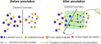
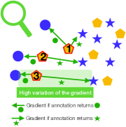
Figure 1: Illustration of the effect of annotation of a target sample selected by SAGE (best viewed in colors). Binary classification problem ($\bullet$ vs $\star$) where source samples are blue and target samples are orange. Before annotation, the class-level alignment is not satisfactory leading to a potential negative transfer (poorly aligned target samples tagged as 1, 2 and 3). We estimate which sample should be annotated as a priority by measuring the variation, before and after annotation, of the gradient of the representations’ transferability. We observe the highest variation is obtained for target sample 3, which is sent to an oracle. The oracle annotation returns class $\star$, validating the suspicion of negative transfer. This leads to an update of the decision boundary which pushes 1, 2 and 3 into class $\star$, resulting of a better class-level alignment of representations.

However, those methods perform significantly worse than their fully supervised counterparts. Practical applications often offer the possibility of annotating a fixed budget of target data; a paradigm referred to as Active Learning (AL). Despite its great practical interest, there are, to our knowledge, only a few previous works which address the problem of Active Domain Adaptation (ADA) (Chattopadhyay et al. 2013; Rai et al. 2010; Saha et al. 2011; Su et al. 2020). In particular, the work of Su et al., proposed recently, is the first that brings active learning to domain adversarial learning.

Our insight is to reserve the annotation budget for the data that will have the most impact on the representations’ transferability. Promoting class-level domain invariance (Long et al. 2018; Bouvier et al. 2020) makes it possible to assess this impact precisely. Indeed, class-level invariance consists of using predicted target labels for soft-class conditioning in the domain adversarial loss. Involving an oracle, which provides the ground-truth, enables to change the contribution of a target sample from soft to hard-class conditioning. Therefore, we measure the impact of annotation by estimating the variation of the domain adversarial loss gradient (see Fig. 1). Thus, in this paper,

• We present Stochastic Adversarial Gradient Embedding (SAGE), an embedding of target samples suited for active learning of domain invariant representations. This embedding is obtained by measuring the variation, before and after annotation, of the domain adversarial loss gradient. SAGE has the following properties:

  1. It takes into account the uncertainty on a target sample label by considering the gradient as a stochastic vector. Since annotation removes uncertainty, it allows us to estimate its expected variation due to the annotation.

  2. The higher the gradient variation norm, the more significant is the impact of annotation on the transferability of representations.

• We follow (Ash et al. 2019) for increasing sampling diversity by promoting target samples for which SAGE span on diverse directions using the k-means++ initialization (Arthur and Vassilvitskii 2006).

• We develop a novel training procedure to incorporate active target samples when learning domain invariant representations. It is split into two steps. The first step, called inductive step, aims to update the classifier smoothly to reflect the annotation. A second step, called the transfer step, leverages the classifier update for learning new class-level invariance.

• We conduct an empirical analysis on well-adopted benchmarks of UDA. It demonstrates that our approach improves the state-of-the-art significantly in Active Adversarial Domain Adaptation (Su et al. 2020) on these datasets. All other things being equal, SAGE performs similarly or better than entropy-based uncertainty sampling or random sampling, making it a credible research direction for the design of new active DA algorithms.

The rest of the paper is organized as follows. First, we provide a brief overview of Domain Adversarial Learning for UDA. Importantly, we expose a soft-class conditioning adversarial loss, which reflects the transferability error of domain invariant representations (Bouvier et al. 2020). Second, we motivate the use of Active Learning for enhancing their transferability. Third, we present the details of Stochastic Adversarial Gradient Embedding. Finally, we conduct an empirical investigation on several benchmarks.

Background

Notations.

Let us consider three random variables; $X$ the input data, $Z$ the representations and $Y$ the labels, defined on spaces $\mathcal{X}$, $\mathcal{Z}\subset\mathbb{R}^{d}$ where $d$ is the dimension of the representation, and $\mathcal{Y}$, respectively. We note realizations with lower cases, $x$, $z$ and $y$, respectively. Those random variables may be sampled from two and different distributions: the source distribution $p_{S}(X,Z,Y)$ i.e., data where the model is trained and the target distribution $p_{T}(X,Z,Y)$ i.e., data where the model is evaluated. Labels are one-hot encoded i.e., $y\in[0,1]^{c}$ with $\sum_{i}y_{i}=1$ where $c$ is the number of classes. We use the index notation $S$ and $T$ to differentiate source and target quantities. We define the hypothesis class $\mathcal{H}$ as a subset of functions from $\mathcal{X}$ to $\mathcal{Y}$ which is the composition of a representation class $\Phi$ (mappings from $\mathcal{X}$ to $\mathcal{Z}$) and a classifier class $\mathcal{F}$ (mappings from $\mathcal{Z}$ to $\mathcal{Y}$) i.e., $h:=f\varphi:=f\circ\varphi\in\mathcal{H}$ where $f\in\mathcal{F}$ and $\varphi\in\Phi$. For $D\in\{S,T\}$ and an hypothesis $h\in\mathcal{H}$, we introduce the risk in domain $D$, $\varepsilon_{D}(h):=\mathbb{E}_{D}[\ell(h(X),Y)]$ where $\ell$ is the $L^{2}$ loss $\ell(y,y^{\prime})=||y-y^{\prime}||^{2}$ and $h(x)_{i}$ is the probability of $x$ to belong to class $i$. We note the source domain data $(x_{i}^{S},y_{i}^{S})_{1\leq i\leq n_{S}}$ and the target domain data $(x_{i}^{T})_{1\leq i\leq n_{T}}$.

Domain Adversarial Learning.

The seminal works from (Ganin and Lempitsky 2015; Ganin et al. 2016; Long et al. 2015), and their theoretical ground (Ben-David et al. 2007, 2010), have led to a wide variety of methods based on domain invariant representations (Long et al. 2016, 2017, 2018; Liu et al. 2019; Chen et al. 2019a; Combes et al. 2020). A representation $\varphi$ and a classifier $f$ are learned by achieving a trade-off between source classification error and domain invariance of representations by fooling a discriminator trained to separate the source from the target domain:

$$\mathcal{L}(\varphi,f):=\mathcal{L}_{\mathrm{c}}(\varphi,f)-\lambda\cdot\inf_{d\in\mathcal{D}}\mathcal{L}_{\mathrm{inv}}(\varphi,d)$$ (1)

where $\mathcal{L}_{\mathrm{c}}(\varphi,f):=\mathbb{E}_{x,y\sim p_{S}}[-y\cdot\log(f\varphi(x))]$ is the cross-entropy loss in the source domain, $\mathcal{L}_{\mathrm{inv}}(\varphi,d):=\mathbb{E}_{x\sim p_{S}}[\log(1-d(\varphi(x)))]+\mathbb{E}_{x\sim p_{T}}[\log(d(\varphi(x))]$ is the adersarial loss and $\mathcal{D}$ is the set of discriminators i.e. mapping from $\mathcal{Z}$ to $[0,1]$. In practice, $\inf_{d\in\mathcal{D}}$ is approximated using a Gradient Reversal Layer (Ganin and Lempitsky 2015).

Transferability loss for class-level invariance.

Promoting class-level domain invariance improves transferability of representations (Long et al. 2018). Recently, Bouvier et al. introduce the transferability loss, noted $\mathcal{L}_{\mathrm{tsf}}$, which performs class-conditioning in the adversarial loss by computing a scalar product between labels $y$ and a class-level discriminator $\mathsf{d}$ defined as a mapping from $\mathcal{Z}$ to $[0,1]^{c}$. Since labels are not available in the target domain at train time, predicted labels $\hat{y}:=f\varphi(x)$ are used. This approach is referred to as soft-class conditioning:

$$\mathcal{L}(\varphi,f):=\mathcal{L}_{\mathrm{c}}(\varphi,f)-\lambda\cdot\inf_{\mathsf{d}\in\mathsf{D}}\mathcal{L}_{\mathrm{tsf}}(\varphi,\hat{y},\mathsf{d})$$ (2)

where $\mathcal{L}_{\mathrm{tsf}}(\varphi,\hat{y},\mathsf{d}):=\mathbb{E}_{(y,x)\sim p_{S}}[y\cdot\log(1-\mathsf{d}(\varphi(x)))]+\mathbb{E}_{(\hat{y},x)\sim p_{T}}[\hat{y}\cdot\log(\mathsf{d}(\varphi(x))]$ is the transferability loss and $\mathsf{D}$ is the the set of class-level discriminators i.e. mappings from $\mathcal{Z}$ to $[0,1]^{c}$. In this work, we explore the role of active annotation of a small subset of the target domain in order to improve the transferability of representations.

Theoretical Analysis

Naive active classifier.

We consider $\mathcal{A}\subset\mathcal{X}$ a measurable subset of $\mathcal{X}$ with probability $b:=p_{T}(X\in\mathcal{A})$. The subset $\mathcal{A}$ is given to an oracle which provides the ground-truth: $y\sim\mathrm{Oracle}(x)$ where $x\in\mathcal{A}$. In concrete terms, $b$ reflects our annotation budget. Given a hypothesis $h\in\mathcal{H}$, we introduce a naive classifier $h_{\mathcal{A}}$ that returns the predicted label $h(x)$ if $x$ is not annotated and the Oracle annotation if $x$ is in the subset $\mathcal{A}$. Thus,

$$h_{\mathcal{A}}(x)=\mathrm{Oracle}(x)\mbox{ if }x\in\mathcal{A},h(x)\mbox{ otherwise.}$$ (3)

To measure the quality of the active set $\mathcal{A}$, we introduce the notion of purity. In particular, we are interested in the amount of information coming from the Oracle. The purity is thus defined as $\pi:=p_{T}\left(h(X)\neq\mathrm{Oracle}(X)\right|X\in\mathcal{A})$ and reflects our capacity to identify misclassified target samples. With this notion, we observe the naive classifier improves the target error:

$$\varepsilon_{T}\left(h_{\mathcal{A}}\right)\leq\varepsilon_{T}(h)-b\pi$$ (4)

The higher the budget of annotation $b$ and the higher the purity $\pi$, the lower the target error of the naive classifier.

The naive classifier as a Transferability Inductive Bias.

We now show how the target error of the naive classifier $\varepsilon_{T}\left(h_{\mathcal{A}}\right)$ is related to the source error of a classifier trained on source labelled data $\varepsilon_{S}(h)$, the annotation budget $b$, the purity of the annotated subset $\pi$, and the transferability of representations $\tau$. We build on the work of Bouvier et al. by interpreting the naive classifier as an inductive bias. More precisely, the naive classifier’s target error is bounded as follows (see supplemental material for the proof):

$$\varepsilon_{T}(h_{\mathcal{A}})\leq\left(\frac{1}{b\pi}-1\right)(\varepsilon_{S}(h)+8\tau+\eta)$$ (5)

where $\tau:=\sup_{\mathsf{f}\in\mathsf{F}}\{\mathbb{E}_{x\sim p_{T}}\left[h_{\mathcal{A}}(x)\cdot\mathsf{f}(\varphi(x))\right]-\mathbb{E}_{x,y\sim p_{S}}[y\cdot\mathsf{f}(\varphi(x))]\}$ is the transferability error, $\mathsf{F}$ is the set of continuous functions from $\mathcal{Z}$ to $[-1,1]^{C}$ and $\eta:=\inf_{\mathsf{f}\in\mathsf{F}}\varepsilon_{T}(\mathsf{f}\varphi)$. It is important to note that the transferability loss $\mathcal{L}_{\mathrm{tsf}}(\varphi,\hat{y}_{\mathcal{A}},\mathrm{d})$ is a domain adversarial proxy of the transferability error $\tau$ where $\hat{y}_{\mathcal{A}}=h_{\mathcal{A}}(x)$ (Bouvier et al. 2020). Interestingly, target labels are only involved in $\pi$ and $\eta$ where the latter is an incompressible error that we assume to be small. The target error of the active classifier is a decreasing function of both the purity and the annotation budget and an increasing function of the transferability error.

Proposed Method

We first expose our motivations to embed target samples using the gradient of the transferability loss. Indeed, this quantity allows to assess the impact of annotation on representations transferability. Second, we define the Stochastic Adversarial Gradient Embedding (SAGE), an embedding where the norm quantifies this impact efficiently. Third, we increase the diversity of sampling in this space, as described in (Ash et al. 2019). Finally, we detail the procedure for the active learning of domain invariant representations.

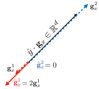
(a) Positive orth. projection

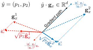
(b) SAGE

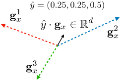
(c) Poor local minimum

Figure 2: (a) The positive orthogonal projection cancels the gradient when the annotation agrees with the prediction. It doubles its norm when the annotation disagrees with the prediction. (b) Visualisation of $\mathrm{SAGE}(x)=(\sqrt{p_{1}}\tilde{\mathbf{g}}_{x}^{1},\sqrt{p_{2}}\tilde{\mathbf{g}}_{x}^{2})$. Here $\tilde{\mathbf{g}}_{x}^{2}\perp\mathbf{g}_{x}^{2}$ since $\hat{y}\cdot\mathbf{g}_{x}$ and $\mathbf{g}_{x}^{2}$ have a similar direction while $|\tilde{\mathbf{g}}_{x}^{1}\cdot\mathbf{g}_{x}|\geq|\mathbf{g}_{x}^{1}\cdot\mathbf{g}_{x}|$ since $\mathbf{g}_{x}^{1}$ as a component in the opposite direction of $\hat{y}\cdot\mathbf{g}_{x}$. (c) Illustration of a case where the transferability loss is close to a local minimum ($\hat{y}\cdot\mathbf{g}_{x}\approx 0$), but the stochastic gradients ($\mathbf{g}_{x}^{y}$ for $y\in\{1,2,3\}$) have a high norm. Here, the annotation chooses one of the gradients resulting in a strong update of the model.

Motivations

As shown in the theoretical section, the budget $b$, the purity $\pi$ and the transferability of representations $\tau$ are levers to improve the naive classifier target error. The budget $b$ must be considered as a cost constraint and not as a parameter to be optimized. The purity of $\pi$ is not tractable since it involves labels in the target domain. Therefore, we focus our efforts on understanding the role of active annotation in improving transferability error $\tau$. Given a target sample $x\sim p_{T}(X)$ with representation $z:=\varphi(x)\in\mathbb{R}^{d}$, we expose the effect of annotating the sample $x$ on the gradient descent update of Eq. 2. To conduct the analysis, we introduce the adversarial gradient $\mathbf{g}_{x}$ of sample $x$ as the gradient of the discriminator loss with respect to the representation $z$:

$$\mathbf{g}_{x}:=-\frac{\partial\log(\mathsf{d}(z))}{\partial z}\in\mathbb{R}^{c\times d},~{}~{}\mbox{where }\mathsf{d}(z)\in[0,1]^{c}$$ (6)

Following the expression of the transferability loss $\mathcal{L}_{\mathrm{tsf}}$, the contribution of a sample $x$ to the gradient update (Eq. 2), before and after its annotation, is:

$$\underbrace{\left\{\theta\leftarrow\theta-\alpha\frac{\partial z}{\partial\theta}\cdot\left(\hat{y}\cdot\mathbf{g}_{x}\right)\right\}}_{\mbox{{Before annotation}}}\underset{}{\longrightarrow}\underbrace{\left\{\theta\leftarrow\theta-\alpha\frac{\partial z}{\partial\theta}\cdot\left(y\cdot\mathbf{g}_{x}\right)\right\}}_{\underset{y\sim\mathrm{Oracle}(x)}{\mbox{{After annotation}}}}$$

where $\partial z/\partial\theta$ is the jacobian of the representations with respect to the deep network parameters $\theta$ i.e., $z:=\varphi_{\theta}(x)$, $\hat{y}:=g\varphi_{\theta}(x)$ is the current label estimation and $\alpha$ is some scaling parameter. Before the annotation, the gradient vector can be written as a weighted sum of $\mathbf{g}_{x}$ i.e., $\hat{y}\cdot\mathbf{g}_{x}\in\mathbb{R}^{d}$, reflecting the class probability of $x$. Annotating the sample $x$ has the effect of setting, once and for all, a direction in $\mathbb{R}^{c}$ of the gradient ($y\cdot\mathbf{g}_{x}$). Based on this observation, we can measure the annotation procedure’s ability to learn more transferable representation by its tendency to change the path of the gradient descent i.e., how $y\cdot\mathbf{g}_{x}$ may differ with $\hat{y}\cdot\mathbf{g}_{x}$.

Positive orthogonal projection

The adversarial gradient $\mathbf{g}_{x}:=\partial\log(\mathsf{d}(z))/\partial z\in\mathbb{R}^{c\times d}$ embodies the uncertainty on the true labels in the first dimension $\mathbb{R}^{c}$. In the rest of the paper, we now consider $\mathbf{g}_{x}$ as a stochastic vector of $\mathbb{R}^{d}$ with realizations lying in a discrete support $\mathcal{G}_{x}:=\{\mathbf{g}_{x}^{1},...,\mathbf{g}_{x}^{c}\}$ where $\mathbf{g}_{x}^{i}=(\partial\log(\mathsf{d}(z))/\partial z)_{i}$. When provided the label through an oracle i.e., $y\sim\mathrm{Oracle}(x)$, we obtain $\mathbf{g}_{x}^{y}\in\mathcal{G}_{x}$, a realization of $\mathbf{g}_{x}$. Before annotation, the direction of the gradient is the mean of $\mathbf{g}_{x}$ where $\mathcal{G}_{x}$ is provided with a probability measure given by the classifier $h(x)$ i.e., $p(\tilde{\mathbf{g}}_{x}=\tilde{\mathbf{g}}_{x}^{i})=h(x)_{i}$:

$$\mathbb{E}_{h}[\mathbf{g}_{x}]:=\mathbb{E}_{y\sim h(x)}\left[\mathbf{g}_{x}^{y}\right]\in\mathbb{R}^{d}$$ (7)

Therefore, the tendency to modify the direction of the gradient is reflected by a high discrepancy between $\mathbb{E}_{h}[\mathbf{g}_{x}]$ and $\mathbf{g}_{x}^{y}$ for $y\sim\mathrm{Oracle}(x)$. To quantify this discrepancy, we consider variations in both direction and magnitude:

• Direction: A simple way to learn a new model by gradient descent is to find samples which modify the gradient’s direction drastically.

• Magnitude: The higher the norm of the gradient, the stronger the update of the model.

To find a good trade-off between direction and magnitude, we remove the mean direction of the gradient $\mathbb{E}_{h}[\mathbf{g}_{x}]$ to $\mathbf{g}_{x}$ by computing a positive orthogonal projection:

$$\tilde{\mathbf{g}}_{x}:=\mathbf{g}_{x}-\lambda\mathbb{E}_{h}[\mathbf{g}_{x}]$$ (8)

where $\lambda:=|\mathbf{g}_{x}\cdot\mathbb{E}_{h}[\mathbf{g}_{x}]|/||\mathbb{E}_{h}[\mathbf{g}_{x}]||^{2}$. Note that we use $|\mathbf{g}_{x}\cdot\mathbb{E}_{h}[\mathbf{g}_{x}]|$, rather than $\mathbf{g}_{x}\cdot\mathbb{E}_{h}[\mathbf{g}_{x}]$ for the standard orthogonal projection, hence its name of positive orthogonal projection.

On the one hand, if the annotation provides a gradient with the same direction as the expected gradient i.e., the annotation reinforces the prediction, $\tilde{\mathbf{g}}_{x}$ is null. On the other hand, if the annotation provides a gradient with an opposite direction to the expected gradient i.e., the annotation contradicts the prediction, the norm of $\tilde{\mathbf{g}}_{x}$ increases. Therefore, target samples $x$ for which we expect the highest impact on the transferability, are those with the highest norm of $\tilde{\mathbf{g}}_{x}$. An illustration is provided in Fig. 2(a). Since $\tilde{\mathbf{g}}_{x}$ is random, we need additional tools to define a norm operator properly on it, leading to our core contribution.

Stochastic Adversarial Gradient Embedding

A simple way to define the norm of $\tilde{\mathbf{g}}_{x}$ would be to consider $||\tilde{\mathbf{g}}_{x}||_{h}:=(\mathbb{E}_{y\sim h(x)}\left[||\tilde{\mathbf{g}}_{x}^{y}||^{2}\right])^{1/2}$ i.e., the expected norm of $\tilde{\mathbf{g}}_{x}$. This leads to a ”distance” defined as follows $(\mathbb{E}_{y_{1}\sim h(x_{1}),y_{2}\sim h(x_{2})}\left[||\mathbf{g}_{x_{1}}^{y_{1}}-\mathbf{g}_{x_{2}}^{y_{2}}||^{2}\right])^{1/2}$. However, it is straightforward to observe such a ”distance” between $\tilde{\mathbf{g}}_{x}$ and itself is not null if $h(x)$ is not a one-hot vector; not making it, in fact, a proper distance.

To address this issue, we suggest to embed, through a mapping named Stochastic Adversarial Gradient Embedding ($\mathrm{SAGE}$), the coupling $(h,\tilde{\mathbf{g}})$ in a vectorial space by considering the following tensorial product:

$$\mathrm{SAGE}(x):=(\sqrt{h(x)_{1}}\tilde{\mathbf{g}}_{x}^{1},...,\sqrt{h(x)_{c}}\tilde{\mathbf{g}}_{x}^{c})\in\mathbb{R}^{c\times d}$$ (9)

Importantly, the choice of using $\sqrt{h}$ is motivated by the observation that $||\mathrm{SAGE}(x)||=||\tilde{\mathbf{g}}_{x}||_{h}$ leading to a proper distance between $x_{1}$ and $x_{2}$:

$$\Delta_{h}(x_{1},x_{2}):=||\mathrm{SAGE}(x_{1})-\mathrm{SAGE}(x_{2})||$$ (10)

Crucially, both the norm and the distance computed on SAGE do not involve the target labels, making it relevant in the UDA setting where target labels are unknown. An illustration of SAGE is provided in Fig. 2(b).

Increasing Diversity of SAGE

As aforementioned, the higher the norm of $||\mathrm{SAGE}(x)||$, the greater the expected impact of annotating sample $x$ on the transferability of representations. A naive strategy of annotation would be simply to rank target samples by their SAGE norm ($||\mathrm{SAGE}(x)||$). However, this strategy ignores the crucial problem of diversity when running active annotation (Settles 2009). Embedding target samples offers the opportunity to increase sampling diversity by selecting samples with high expected norms and various directions (Ash et al. 2019). The k-means++ initialization is known to select diverse and high norm vectors. Roughly speaking, the algorithm starts by selecting the vectors $v$ with the highest norm and the second, $v^{\prime}$, such that $v^{\prime}-v$ has the highest norm, and so on. The procedure is detailed in Algorithm 1.

Algorithm 1 diverse_SAGE$((x_{i}^{T})_{1\leq i\leq n_{T}},f,\varphi,\mathsf{d},b)$

Input: Target samples $(x_{i}^{T})_{1\leq i\leq n_{T}}$, classifier $f$, representation $\varphi$, discriminator $\mathsf{d}$, budget $b$:

1:  $\mathcal{A}\leftarrow\mathtt{[}\arg\max_{1\leq i\leq n_{T}}||\tilde{\mathbf{g}}_{x_{i}^{T}}||_{h}\mathtt{]}$

2:  while $\mathtt{len}(\mathcal{A})<b$ do

3:     $\mathcal{A}\mathtt{.append}\left(\displaystyle{\arg\max_{1\leq i\leq n_{t}}\min_{a\in\mathcal{A}}\Delta_{f\varphi}(x_{i}^{T},x_{a}^{T})}\right)$

4:  end while

5:  Return $\mathcal{A}$

Training procedure

The training procedure is described in Algorithm 2. First, we train the model by UDA (Bouvier et al. 2020). Second, for a given number of iterations, we select by SAGE $b$ samples to send to the Oracle. Then, we perform two steps: an inductive step and a transfer step. The former updates the current classifier, for learning an active classifier, by incorporating the knowledge provided by annotated samples. The latter updates the representations for achieving class-level invariance where the predictions of the active classifier are used in the target domain. This procedure is repeated for the $r$ annotation rounds. In the following, we note $h_{a}\in\mathcal{H}$ an active classifier i.e., a classifier that takes into account annotations provided by the Oracle (e.g., the naive classifier).

Transfer step.

Based on our theoretical analysis, the representations transferability is improved when $h_{a}$ is introduced into the transferability loss:

$$\mathcal{L}_{\mathrm{tsf}}(\varphi,h_{a},\mathsf{d}):= ~{}\mathbb{E}_{(y,x)\sim p_{S}}[y\cdot\log(1-\mathsf{d}(\varphi(x)))]$$

$$~{}+\mathbb{E}_{x\sim p_{T}}[h_{a}(x)\cdot\log(\mathsf{d}(\varphi(x))]$$ (11)

The active classifier is involved in the target domain to compute the transferability loss. Therefore, we introduce the Transfer step which consists in the following stochastic gradient descent update:

$$\mbox{{transfer}}(f,\varphi,h_{a}):= (f,g)-\alpha\nabla_{(f,g)}\{\mathcal{L}_{\mathrm{c}}(\varphi,f)$$

$$-\lambda\cdot\inf_{\mathsf{d}\in\mathsf{D}}\mathcal{L}_{\mathrm{tsf}}(\varphi,h_{a},\mathsf{d})\}$$ (12)

where $\inf_{\mathsf{d}\in\mathsf{D}}$ is in practice a gradient reversal layer (Ganin and Lempitsky 2015), $\alpha$ is scaling parameter, $\lambda$ varies smoothly from $0$ to $1$ during training as described in (Long et al. 2018) and losses are computed on batches of samples.

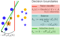
Figure 3: Illustration of the decision boundary update when varying the inductive design of the active classifier. Sample 2 is sent to an Oracle providing annotation $\star$ when the current classifier $h$ predicts $\bullet$. Based on this annotation, one can assume strongly that 1 is a $\star$. Here, the naive classifier predicts $\bullet$ for 1. Both 1 and 2 are close to the balance classifier’s decision boundary due to a $\bullet$ source sample 3 resulting in an uncertain predictions, thus a poor class-conditioning in the transferability loss. Our inductive step allows to obtain confident predictions for both 1 and 2. The active classifier misclassifies 3 enforcing the model to learn a better-suited representation for 3, improving the representation alignment.

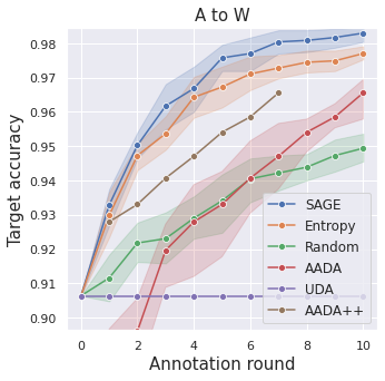
(a) A$\to$W

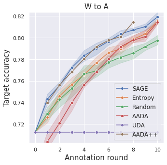
(b) W$\to$A

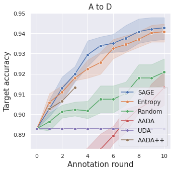
(c) A$\to$D

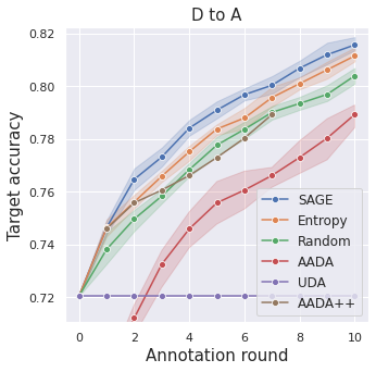
(d) D$\to$A

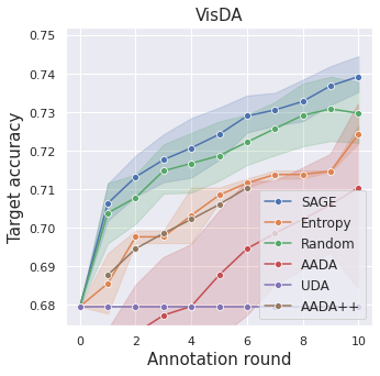
(e) VisDA($b=10$)

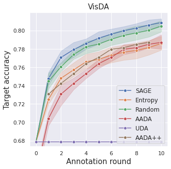
(f) VisDA($b=100$)

Figure 4: SAGE outperforms the baselines for the six tasks. Annotation of target samples improves the transferability of domain invariant representations drastically. If uncertainty-based selection (Entropy) performs better than diversity-based selection (Random) for the Office31 dataset, the opposite is observed for the VisDA dataset. For both datasets, SAGE performs better than both uncertainty and diversity-based selections, demonstrating its capacity to take the best of the two worlds.

Algorithm 2 Training procedure

Input: Target samples $(x_{i}^{T})_{1\leq i\leq n_{T}}$, annotation budget $b$, annotation rounds $r$, iterations $n_{\mathrm{it}}$:

1:  $f,\varphi\leftarrow$ UDA pretraining, $\mathcal{A}\leftarrow\mathtt{[}~{}\mathtt{]}$.

2:  for $r$ rounds of annotations do

3:     $\mathcal{A}\mathtt{.append(}\mbox{{diverse\_SAGE}}((x_{i}^{T})_{1\leq i\leq n_{T}},f,\varphi,\mathsf{d},b)\mathtt{)}$ # Annotate target samples selected by diverse SAGE.

4:     for  $n_{\mathrm{it}}$ iterations do

5:        $h_{a}\leftarrow\mbox{{inductive}}(f\varphi,\mathcal{A})$ # Inductive step: annotations are incorporated in the active classifier.

6:        $(f,\varphi)\leftarrow\mbox{{transfer}}(f,\varphi,h_{a})$ # Transfer step: representation and classifier update for aligning with the feedback of the active classifier.

7:     end for

8:  end for

Inductive step.

We now focus our attention on the design of the active classifier $h_{a}$, referred to as the Inductive step, as described in (Bouvier et al. 2020). Our theoretical analysis from Eq. 5 holds for the naive classifier (it outputs the oracle annotation if the target sample is annotated and the current prediction otherwise). However, given two samples $x_{1}$ and $x_{2}$ close in the representation space i.e., $z_{1}\approx z_{2}$, such that $x_{1}$ is annotated, $y_{1}\sim\mathrm{Oracle}(x_{1})$, one can assume that the probability of observing $y_{1}=\mathrm{Oracle}(y_{2})$ is high. However, the design of the naive classifier does not reflect this inductive bias since $h_{\mathcal{A}}(x_{2})=h(x_{2})$ (see Fig. 3). Therefore, we suggest to train an active classifier based on the annotation provided by the Oracle to spread the information in the representation space neighborhood of $x_{1}$. We propose to use a simple loss that incorporates both the error in the source domain and the error in target annotated samples as follows:

$$h_{a}:=\arg\min_{h\in\mathcal{H}}\gamma\mathcal{L}_{\mathrm{c}}(h)+(1-\gamma){\mathcal{L}}_{\mathcal{A}}(h)$$ (13)

where ${\mathcal{L}}_{\mathcal{A}}(h)=\mathbb{E}_{x\in\mathcal{A}}[-\mathrm{Oracle}(x)\cdot\log(h(x))]$ and $\gamma\in(0,1)$ is a trade-off parameter. On the one hand, when the annotated samples have high importance to learn $h_{a}$ i.e., $\gamma$ tends to 0, we are exposed to a high risk of high variance of such classifier since $|\mathcal{A}|\ll n_{S}$. On the other hand, when the source samples have a high importance to learn $h_{a}$ i.e., $\gamma$ tends to 1, knowledge provided by the annotation is poorly learned by the active classifier. Therefore, calibrating properly $\gamma$ is a challenging problem. We overcome this issue by smoothly updating the classifier $h$ as follows:

$$\mbox{{inductive}}(h,\mathcal{A}):=h-\alpha\nabla_{h}{\mathcal{L}}_{\mathcal{A}}(h)$$ (14)

The design of inductive aims not to forget knowledge acquired in the source domain while integrating the knowledge provided by the annotation of the target samples.

Experiments

Datasets.

We evaluate our approach on Office-31 (Saenko et al. 2010) and VisDA-2017 (Peng et al. 2017). Office-31 contains 4,652 images classified in 31 categories across three domains: Amazon (A), Webcam (W), and DSLR (D). We explore tasks $\textbf{A}\to\textbf{W}$, $\textbf{W}\to\textbf{A}$, $\textbf{A}\to\textbf{D}$ and $\textbf{D}\to\textbf{A}$. We do not report results for tasks $\textbf{D}\to\textbf{W}$ and $\textbf{W}\to\textbf{D}$ since these tasks have already nearly perfect results in UDA (Long et al. 2018). For VisDA, we explore Synthetic: 3D models with different lightning conditions and different angles; Real: real-world images. We explore the Synthetic $\rightarrow$ Real task. The standard protocol in UDA uses the same target samples during train and test phases. In the context of active learning, this induces an undesirable effect where sample annotation mechanically increases the accuracy; at train time, the model has access to input and label of annotated samples which are also present at test time. We suggest instead to split the target domain into a train target domain (samples used for adaptation and pool of data used for annotation) and test target domain (samples used for evaluating the model) with a ratio of $1/2$. Therefore, samples from the test target domain have never been seen at train time.

Setup.

For classification, we use the same hyperparameters than (Long et al. 2018) and adopt ResNet-50 (He et al. 2016) as a base network pre-trained on ImageNet dataset (Deng et al. 2009). Our code is based on official implementations of Bouvier et al. derived from (Long et al. 2018). For all experiments, we have fixed $r=10$ rounds of annotations. For Office31, we have fixed a budget of $b=2\%$ of annotation of the train target domain i.e., $20\%$ of the train target domain is annotated at the end of the 10 rounds. For VisDA, we have explored two budgets: $b=10$ or $100$ samples. We report average results obtained with 6 random experiments. We perform 10k iterations of SGD for the UDA pre-training while, between each annotation round, we perform 5k iterations of SGD. One experiment lasts about $\sim$12 hours on a single NVIDIA V100 GPU with 32GB memory. The full implementation is provided in the supplemental material.

Baselines.

AADA (Su et al. 2020) is the closest algorithm to SAGE and the most interesting to compare. AADA learns domain invariant representations by fooling a domain discriminator $d$ trained to output 1 for source data and 0 for target data (Ganin and Lempitsky 2015) and scores target samples $x$; $s(x):=H(\hat{y})w(z)$ where $H(\hat{y})$ is the entropy of predictions $\hat{y}$ and $w(z)=(1-d(z))/d(z)$. $H(\hat{y})$ brings information about uncertainty while $w(z)$ brings diversity to the score. We have reproduced the implementation of AADA. SAGE starts active learning with a serious advantage to AADA as the pre-training procedures differ significantly. In order to get a fairer comparison with SAGE, we have therefore chosen to report a modified version of AADA that we call AADA++. AADA++ is free of charge as long as the performance is below the UDA baseline (Bouvier et al. 2020) (UDA). In our view, this should essentially eliminate AADA’s structural disadvantage. In practical terms, we translate AADA to the left of the graph $\mathrm{(Annotation~{}round,Target~{}accuracy)}$ until accuracy at request 0 is higher than UDA, explaining why annotation rounds of AADA++ do not reach 10. We also report Entropy (uncertainty-based sampling which selects samples with the highest entropy) and Random (diversity-based sampling which selects samples randomly). For both Entropy and Random baselines, the training procedure of Algorithm 2 is followed, except for line 3 where SAGE is replaced by entropy sampling (Wang and Shang 2014) or random sampling.

Results.

We report the results of experiments in Fig. 4. Approximately 110 days of GPU time are necessary for reproducing the results. First, active annotation brings substantial improvements to UDA for both datasets. This validates the effort and the focus that should be put on active domain adaptation in our opinion. For the six tasks, SAGE outperforms the baselines (AADA in particular) with a comfortable margin. More precisely, the saturation regime for AADA for A$\to$W, D$\to$A and VisDA tasks is significantly below than the saturation regime of SAGE. Even when provided with free annotation rounds, AADA++ is less accurate than SAGE, except for task W$\to$A, demonstrating the significant improvement made by SAGE. In addition, we observe that AADA is unstable when only few data are annotated (VisDA($b=10$)), while SAGE remains robust in this regime. Finally, uncertainty-based sampling (Entropy) performed better than diverse-based sampling (Random) for the Office31 dataset, while the contrary is observed for the VisDA dataset. Interestingly, SAGE performs better than both Entropy and Random, showing that SAGE takes the best of both worlds (uncertainty vs diversity).

Ablation study.

We conduct an ablation study to compare the inductive step described in Eq. 14 with a step based on Eq. 13 (Balance with $\gamma=0.5$) or based on Eq. 3 (Naive). We report results for tasks A$\to$W, W$\to$A and both tasks of VisDA($b=100$). We observe that both Balance and Inductive improve significantly performances compared to the Naive classifier, demonstrating the importance of the inductive step. For both tasks A$\to$W and W$\to$A, Inductive is slightly better than Balance, confirming our belief that smooth updating the classifier (as described in Eq. 14) improves performances. Interestingly, Inductive performed better than Balance when few data are annotated (e.g., VisDA with $b=10$, VisDA with $b=100$ for rounds lower than 3), while the contrary was observed when more data is annotated. This findings tend to show that Inductive is more adapted in the low annotation regime. All things considered, the difference between Balance and Inductive remains small compared to the improvement provided by SAGE compared to AADA. Nevertheless, the inductive step remains an important step in SAGE and deserves a deeper understanding. More ablation is provided in the Appendix.

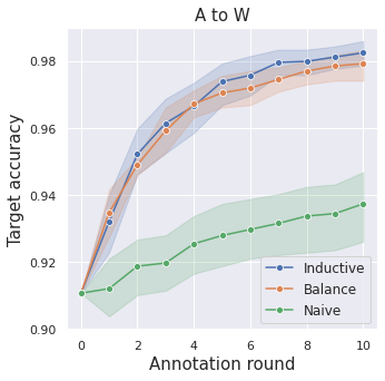
(a) A$\to$W

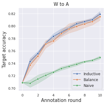
(b) W$\to$A

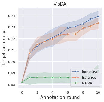
(c) VisDA($b=10$)

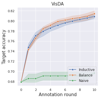
(d) VisDA($b=100$)

Figure 5: Both Inductive and Balance improve the active learning compared with the Naive classifier. Inductive seems to provide better guarantees compared with the Balance classifier when only few data are annotated. This remark opens the way to interesting future work in ADA.

We demonstrate the effectiveness of k-means++ (Arthur and Vassilvitskii 2006) in SAGE. Additionally to report SAGE (SAGE with k-means++), we also reports results of Active Domain Adaptation when target samples are selected with respect to their SAGE norm ($||\mathrm{SAGE}||$), thus not taking in account directions of gradients. Results are presented in Fig. 6 for tasks A$\to$W, W$\to$A and both tasks of VisDA($b=10$ and $100$).

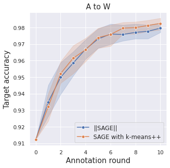
(a) A$\to$W

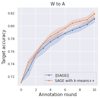
(b) W$\to$A

(c) VisDA($b=10$)

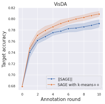
(d) VisDA($b=100$)

Figure 6: For the four tasks selected for the ablation study, the k-means++ initialization brings substantial improvments especially for tasks W$\to$A and VisDA for $b=10$ and $100$.

Related works

Transferability of Invariant Representations.

Recent works warn that domain invariance may deteriorate transferability of invariant representations (Johansson, Sontag, and Ranganath 2019; Zhao et al. 2019). Prior works enhance their transferability with multi-linear conditioning of representations with predictions (Long et al. 2018), by introducing weights (Cao et al. 2018; Bouvier et al. 2019; You et al. 2019; Zhang et al. 2018; Combes et al. 2020), by penalizing high singular value of representations batch (Chen et al. 2019b), by hallucinating consistent target samples for bridging the domain gap (Liu et al. 2019) or by enforcing target consistency through augmentations which conserve the semantic of the input (Ouali et al. 2020).

Active Learning.

There is an extensive literature on Active Learning (Settles 2009) that can be divided into two schools; uncertainty and diversity. The first aims to annotate samples for which the model has uncertain prediction e.g., samples are selected according to their entropy (Wang and Shang 2014) or prediction margin (Roth and Small 2006), with some theoretical guarantees (Hanneke et al. 2014; Balcan, Beygelzimer, and Langford 2009). The second focuses on annotating a representative sample of the data distribution e.g., the Core-Set approach (Sener and Savarese 2017) selects samples that geometrically cover the distribution. Several approaches also propose a trade-off between uncertainty and diversity, e.g., (Hsu and Lin 2015) that is formulated as a bandit problem. Recently, Ash et al. introduced BADGE, a gradient embedding, which, like SAGE, takes the best of uncertainty and diversity. Our work is inspired by BADGE and adapts the core ideas in the context of learning domain invariant representations.

Active Domain Adaptation.

Despite its great practical interest, only a few previous works address the problem of Active Domain Adaptation. (Chattopadhyay et al. 2013) annotates target samples by importance sampling while ALDA (Rai et al. 2010; Saha et al. 2011) annotates samples with high discrepancy with source samples based on the prediction of a domain discriminator. However, those strategies do not fit modern adaptation with deep nets. To our knowledge, AADA (Su et al. 2020) is the only prior work that learns actively domain invariant representations and achieves the state-of-the-art for Active Domain Adaptation. Thus, AADA is the most relevant work to compare with SAGE.

Conclusion

We have introduced SAGE, an efficient method for active adversarial domain adaptation. SAGE is an embedding suitable for identifying target samples that are likely to improve representations’ transferability when annotated. It relies on three core components; a stochastic embedding of the gradient of the transferability loss, a k-means++ initialization which guarantees that each annotation round annotates a diverse set of target samples, and a two-step learning procedure that incorporates efficiently active target samples when learning invariant representations. Through various experiments, we have demonstrated the effectiveness of SAGE for improving the transferability of representations and its capacity to take the best of uncertainty and diversity sampling.

Appendix A Proof of the theoretical analysis

The naive classifier’s target error is bounded as follows:

$$\varepsilon_{T}(h_{\mathcal{A}})\leq\left(\frac{1}{b\pi}-1\right)(\varepsilon_{S}(h)+8\tau+\eta)$$ (15)

where $\tau:=\sup_{\mathsf{f}\in\mathsf{F}}\{\mathbb{E}_{x\sim p_{T}}\left[h_{\mathcal{A}}(x)\cdot\mathsf{f}(\varphi(x))\right]-\mathbb{E}_{x,y\sim p_{S}}[y\cdot\mathsf{f}(\varphi(x))]\}$ is the transferability error, $\mathsf{F}$ is the set of continuous functions from $\mathcal{Z}$ to $[-1,1]^{C}$ and $\eta:=\inf_{\mathsf{f}\in\mathsf{F}}\varepsilon_{T}(\mathsf{f}\varphi)$.

Proof.

First, we observe that :

$$\varepsilon_{T}(h_{\mathcal{A}})\leq\beta\varepsilon_{T}(h)$$ (16)

with $\beta=1-\frac{b\pi}{\varepsilon_{T}(h)}$. Then;

$$\rho:=\frac{\beta}{1-\beta}=\frac{\varepsilon_{T}(h)}{b\pi}-1\leq\frac{1}{b\pi}-1$$ (17)

We apply Bound 4 from (Bouvier et al. 2020) where the inductive classifier is the active classifer $h_{\mathcal{A}}$. Then we bound the invariance error using the transferability error (Proposition 3, item 1 from (Bouvier et al. 2020)) to obtain $6\tau+2\tau=8\tau$, leading to the announced result. ∎

References

- Amodei et al. (2016) Amodei, D.; Olah, C.; Steinhardt, J.; Christiano, P.; Schulman, J.; and Mané, D. 2016. Concrete problems in AI safety. arXiv preprint arXiv:1606.06565 .
- Arjovsky et al. (2019) Arjovsky, M.; Bottou, L.; Gulrajani, I.; and Lopez-Paz, D. 2019. Invariant Risk Minimization. arXiv preprint arXiv:1907.02893 .
- Arthur and Vassilvitskii (2006) Arthur, D.; and Vassilvitskii, S. 2006. k-means++: The advantages of careful seeding. Technical report, Stanford.
- Ash et al. (2019) Ash, J. T.; Zhang, C.; Krishnamurthy, A.; Langford, J.; and Agarwal, A. 2019. Deep batch active learning by diverse, uncertain gradient lower bounds. arXiv preprint arXiv:1906.03671 .
- Balcan, Beygelzimer, and Langford (2009) Balcan, M.-F.; Beygelzimer, A.; and Langford, J. 2009. Agnostic active learning. Journal of Computer and System Sciences 75(1): 78–89.
- Beery, Van Horn, and Perona (2018) Beery, S.; Van Horn, G.; and Perona, P. 2018. Recognition in terra incognita. In Proceedings of the European Conference on Computer Vision (ECCV), 456–473.
- Ben-David et al. (2010) Ben-David, S.; Blitzer, J.; Crammer, K.; Kulesza, A.; Pereira, F.; and Vaughan, J. W. 2010. A theory of learning from different domains. Machine learning 79(1-2): 151–175.
- Ben-David et al. (2007) Ben-David, S.; Blitzer, J.; Crammer, K.; and Pereira, F. 2007. Analysis of representations for domain adaptation. In Advances in neural information processing systems, 137–144.
- Bouvier et al. (2020) Bouvier, V.; Very, P.; Chastagnol, C.; Tami, M.; and Hudelot, C. 2020. Robust Domain Adaptation: Representations, Weights and Inductive Bias. arXiv preprint arXiv:2006.13629 .
- Bouvier et al. (2019) Bouvier, V.; Very, P.; Hudelot, C.; and Chastagnol, C. 2019. Hidden Covariate Shift: A Minimal Assumption For Domain Adaptation. arXiv preprint arXiv:1907.12299 .
- Buitinck et al. (2013) Buitinck, L.; Louppe, G.; Blondel, M.; Pedregosa, F.; Mueller, A.; Grisel, O.; Niculae, V.; Prettenhofer, P.; Gramfort, A.; Grobler, J.; Layton, R.; VanderPlas, J.; Joly, A.; Holt, B.; and Varoquaux, G. 2013. API design for machine learning software: experiences from the scikit-learn project. In ECML PKDD Workshop: Languages for Data Mining and Machine Learning, 108–122.
- Cao et al. (2018) Cao, Z.; Ma, L.; Long, M.; and Wang, J. 2018. Partial adversarial domain adaptation. In Proceedings of the European Conference on Computer Vision (ECCV), 135–150.
- Chattopadhyay et al. (2013) Chattopadhyay, R.; Fan, W.; Davidson, I.; Panchanathan, S.; and Ye, J. 2013. Joint transfer and batch-mode active learning. In International Conference on Machine Learning, 253–261.
- Chen et al. (2019a) Chen, C.; Xie, W.; Huang, W.; Rong, Y.; Ding, X.; Huang, Y.; Xu, T.; and Huang, J. 2019a. Progressive feature alignment for unsupervised domain adaptation. In Proceedings of the IEEE Conference on Computer Vision and Pattern Recognition, 627–636.
- Chen et al. (2019b) Chen, X.; Wang, S.; Long, M.; and Wang, J. 2019b. Transferability vs. discriminability: Batch spectral penalization for adversarial domain adaptation. In International Conference on Machine Learning, 1081–1090.
- Combes et al. (2020) Combes, R. T. d.; Zhao, H.; Wang, Y.-X.; and Gordon, G. 2020. Domain Adaptation with Conditional Distribution Matching and Generalized Label Shift. arXiv preprint arXiv:2003.04475 .
- Deng et al. (2009) Deng, J.; Dong, W.; Socher, R.; Li, L.-J.; Li, K.; and Fei-Fei, L. 2009. Imagenet: A large-scale hierarchical image database. In 2009 IEEE conference on computer vision and pattern recognition, 248–255. Ieee.
- Ganin and Lempitsky (2015) Ganin, Y.; and Lempitsky, V. 2015. Unsupervised Domain Adaptation by Backpropagation. In International Conference on Machine Learning, 1180–1189.
- Ganin et al. (2016) Ganin, Y.; Ustinova, E.; Ajakan, H.; Germain, P.; Larochelle, H.; Laviolette, F.; Marchand, M.; and Lempitsky, V. 2016. Domain-adversarial training of neural networks. The Journal of Machine Learning Research 17(1): 2096–2030.
- Geva, Goldberg, and Berant (2019) Geva, M.; Goldberg, Y.; and Berant, J. 2019. Are We Modeling the Task or the Annotator? An Investigation of Annotator Bias in Natural Language Understanding Datasets. arXiv preprint arXiv:1908.07898 .
- Hanneke et al. (2014) Hanneke, S.; et al. 2014. Theory of disagreement-based active learning. Foundations and Trends® in Machine Learning 7(2-3): 131–309.
- He et al. (2016) He, K.; Zhang, X.; Ren, S.; and Sun, J. 2016. Deep residual learning for image recognition. In Proceedings of the IEEE conference on computer vision and pattern recognition, 770–778.
- Hsu and Lin (2015) Hsu, W.-N.; and Lin, H.-T. 2015. Active learning by learning. In Twenty-Ninth AAAI conference on artificial intelligence. Citeseer.
- Hunter (2007) Hunter, J. D. 2007. Matplotlib: A 2D graphics environment. Computing in Science & Engineering 9(3): 90–95. doi:10.1109/MCSE.2007.55.
- Johansson, Sontag, and Ranganath (2019) Johansson, F.; Sontag, D.; and Ranganath, R. 2019. Support and Invertibility in Domain-Invariant Representations. In The 22nd International Conference on Artificial Intelligence and Statistics, 527–536.
- Krizhevsky, Sutskever, and Hinton (2012) Krizhevsky, A.; Sutskever, I.; and Hinton, G. E. 2012. Imagenet classification with deep convolutional neural networks. In Advances in neural information processing systems, 1097–1105.
- Liu et al. (2019) Liu, H.; Long, M.; Wang, J.; and Jordan, M. 2019. Transferable Adversarial Training: A General Approach to Adapting Deep Classifiers. In International Conference on Machine Learning, 4013–4022.
- Long et al. (2015) Long, M.; Cao, Y.; Wang, J.; and Jordan, M. I. 2015. Learning transferable features with deep adaptation networks. In Proceedings of the 32nd International Conference on International Conference on Machine Learning-Volume 37, 97–105. JMLR. org.
- Long et al. (2018) Long, M.; Cao, Z.; Wang, J.; and Jordan, M. I. 2018. Conditional adversarial domain adaptation. In Advances in Neural Information Processing Systems, 1640–1650.
- Long et al. (2016) Long, M.; Zhu, H.; Wang, J.; and Jordan, M. I. 2016. Unsupervised domain adaptation with residual transfer networks. In Advances in Neural Information Processing Systems, 136–144.
- Long et al. (2017) Long, M.; Zhu, H.; Wang, J.; and Jordan, M. I. 2017. Deep transfer learning with joint adaptation networks. In Proceedings of the 34th International Conference on Machine Learning-Volume 70, 2208–2217. JMLR. org.
- Marcus (2020) Marcus, G. 2020. The Next Decade in AI: Four Steps Towards Robust Artificial Intelligence. arXiv preprint arXiv:2002.06177 .
- Oquab et al. (2014) Oquab, M.; Bottou, L.; Laptev, I.; and Sivic, J. 2014. Learning and transferring mid-level image representations using convolutional neural networks. In Proceedings of the IEEE conference on computer vision and pattern recognition, 1717–1724.
- Ouali et al. (2020) Ouali, Y.; Bouvier, V.; Tami, M.; and Hudelot, C. 2020. Target Consistency for Domain Adaptation: when Robustness meets Transferability. arXiv preprint arXiv:2006.14263 .
- Pan and Yang (2009) Pan, S. J.; and Yang, Q. 2009. A survey on transfer learning. IEEE Transactions on knowledge and data engineering 22(10): 1345–1359.
- Paszke et al. (2019) Paszke, A.; Gross, S.; Massa, F.; Lerer, A.; Bradbury, J.; Chanan, G.; Killeen, T.; Lin, Z.; Gimelshein, N.; Antiga, L.; et al. 2019. PyTorch: An imperative style, high-performance deep learning library. In Advances in Neural Information Processing Systems, 8024–8035.
- Peng et al. (2017) Peng, X.; Usman, B.; Kaushik, N.; Hoffman, J.; Wang, D.; and Saenko, K. 2017. Visda: The visual domain adaptation challenge. arXiv preprint arXiv:1710.06924 .
- Quionero-Candela et al. (2009) Quionero-Candela, J.; Sugiyama, M.; Schwaighofer, A.; and Lawrence, N. D. 2009. Dataset shift in machine learning. The MIT Press.
- Rai et al. (2010) Rai, P.; Saha, A.; Daumé III, H.; and Venkatasubramanian, S. 2010. Domain adaptation meets active learning. In Proceedings of the NAACL HLT 2010 Workshop on Active Learning for Natural Language Processing, 27–32. Association for Computational Linguistics.
- Roth and Small (2006) Roth, D.; and Small, K. 2006. Margin-based active learning for structured output spaces. In European Conference on Machine Learning, 413–424. Springer.
- Saenko et al. (2010) Saenko, K.; Kulis, B.; Fritz, M.; and Darrell, T. 2010. Adapting visual category models to new domains. In European conference on computer vision, 213–226. Springer.
- Saha et al. (2011) Saha, A.; Rai, P.; Daumé, H.; Venkatasubramanian, S.; and DuVall, S. L. 2011. Active supervised domain adaptation. In Joint European Conference on Machine Learning and Knowledge Discovery in Databases, 97–112. Springer.
- Sener and Savarese (2017) Sener, O.; and Savarese, S. 2017. Active learning for convolutional neural networks: A core-set approach. arXiv preprint arXiv:1708.00489 .
- Settles (2009) Settles, B. 2009. Active learning literature survey. Technical report, University of Wisconsin-Madison Department of Computer Sciences.
- Su et al. (2020) Su, J.-C.; Tsai, Y.-H.; Sohn, K.; Liu, B.; Maji, S.; and Chandraker, M. 2020. Active adversarial domain adaptation. In The IEEE Winter Conference on Applications of Computer Vision, 739–748.
- Vaswani et al. (2017) Vaswani, A.; Shazeer, N.; Parmar, N.; Uszkoreit, J.; Jones, L.; Gomez, A. N.; Kaiser, Ł.; and Polosukhin, I. 2017. Attention is all you need. In Advances in neural information processing systems, 5998–6008.
- Walt, Colbert, and Varoquaux (2011) Walt, S. v. d.; Colbert, S. C.; and Varoquaux, G. 2011. The NumPy array: a structure for efficient numerical computation. Computing in science & engineering 13(2): 22–30.
- Wang and Shang (2014) Wang, D.; and Shang, Y. 2014. A new active labeling method for deep learning. In 2014 International joint conference on neural networks (IJCNN), 112–119. IEEE.
- Yosinski et al. (2014) Yosinski, J.; Clune, J.; Bengio, Y.; and Lipson, H. 2014. How transferable are features in deep neural networks? In Advances in neural information processing systems, 3320–3328.
- You et al. (2019) You, K.; Long, M.; Cao, Z.; Wang, J.; and Jordan, M. I. 2019. Universal domain adaptation. In Proceedings of the IEEE Conference on Computer Vision and Pattern Recognition, 2720–2729.
- Zhang et al. (2018) Zhang, J.; Ding, Z.; Li, W.; and Ogunbona, P. 2018. Importance weighted adversarial nets for partial domain adaptation. In Proceedings of the IEEE Conference on Computer Vision and Pattern Recognition, 8156–8164.
- Zhao et al. (2019) Zhao, H.; Des Combes, R. T.; Zhang, K.; and Gordon, G. 2019. On Learning Invariant Representations for Domain Adaptation. In International Conference on Machine Learning, 7523–7532.