Spectral Variability of Radio Sources at Low Frequencies

Abstract

Spectral variability of radio sources encodes information about the conditions of intervening media, source structure, and emission processes. With new low-frequency radio interferometers observing over wide fractional bandwidths, studies of spectral variability for a large population of extragalactic radio sources are now possible. Using two epochs of observations from the GaLactic and Extragalactic All-sky Murchison Widefield Array (GLEAM) survey that were taken one year apart, we search for spectral variability across 100–230 MHz for 21,558 sources. We present methodologies for detecting variability in the spectrum between epochs and for classifying the type of variability: either as a change in spectral shape or as a uniform change in flux density across the bandwidth. We identify 323 sources with significant spectral variability over a year-long timescale. Of the 323 variable sources, we classify 51 of these as showing a significant change in spectral shape. Variability is more prevalent in peaked-spectrum sources, analogous to gigahertz-peaked spectrum and compact steep-spectrum sources, compared to typical radio galaxies. We discuss the viability of several potential explanations of the observed spectral variability, such as interstellar scintillation and jet evolution. Our results suggest that the radio sky in the megahertz regime is more dynamic than previously suggested.

1 Introduction

Radio source variability is a powerful resource for studying extragalactic source structure and the physics of the environmental interaction of a radio galaxy. The two main categories of variability, intrinsic and extrinsic, provide information about the source itself or the intervening media along the line of sight, respectively. For example, radio variability can inform us about adiabatic expansion from changes in optical depth with time (Tingay et al., 2015) or changes in accretion state and jet evolution (Tetarenko et al., 2019). Extrinsic variability induced by scintillation provides information about the electron density variations between the source and observer. It can also give detailed information on the instrnsic structure of the source, particularly on the smallest angular scales (e.g. Macquart & de Bruyn, 2007). The majority of previous studies of spectral variability have been conducted at gigahertz frequencies, which have shown to be dominated by the contributions from the core and jets (Hardcastle & Looney, 2008), and thus detections of variability in the gigahertz regime have been common (e.g. Quirrenbach et al., 1989; Quirrenbach et al., 1992; Fan, J. H. et al., 2007; Bower et al., 2011).

Intrinsic variability of synchrotron radiation allows an observer to place a strict upper limit on the brightness temperature of the emission (e.g. Miller-Jones et al., 2008). Brightness temperatures for all sources emitting synchrotron radiation are subject to the strict upper limit of $10^{12}$ K due to the Compton scattering limit (Kellermann & Pauliny-Toth, 1969). Sources with temperatures which exceed this limit indicate that their emission is coherent, as in the case of pulsars, or beamed towards the observer, as in the case of blazars.

The magnitude of the brightness modulation and timescales of extrinsic variability are dependent on which intervening medium is causing the scintillation (Hancock et al., 2019) and the source size (Narayan, 1992). Depending on the frequency of the radiation, interstellar scintillation (ISS) typically varies source brightness on timescales of months to years (Coles et al., 1987), and is a result of the intervening electron density in the interstellar medium (ISM). ISS has two subcategories, refractive and diffractive, which produce slow (months–years) and short (days–weeks) timescale variability, respectively (Rickett, 1986). Interplanetary scintillation (IPS) occurs when radio waves are distorted as they travel through the Solar wind (Clarke, 1964; Hewish & Burnell, 1970). Typically IPS has timescales of seconds or shorter, and sources with a larger angular size can vary due to IPS compared to ISS.

Previous studies of variability and transients at low frequencies ($<1$ GHz) have searched a wide range of timescales and types of radio sources since the first discovery of variability due to refractive interstellar scintillation (RISS; Hunstead, 1972; Rickett, 1986; Fanti et al., 1990; Riley, 1993; Hancock et al., 2019). However, such searches have only identified a small population. Chhetri et al. (2018) searched for variability in a sample of compact 37 extragalactic radio sources and identified only one source as showing significant variability; J013243-165444, a known blazar with a peaked radio spectrum.

A comparison of TIFR GMRT 150 MHz Sky Survey Alternative Data Release 1 (TGSS-ADR1; Intema, H. T. et al., 2017) and the GaLactic and Extragalactic All-Sky Murchison Widefield Array (GLEAM; Wayth et al., 2015; Hurley-Walker et al., 2017b) surveys at $\sim 150$ MHz to search for transients between the two surveys yielded only one candidate that had no detectable spectral curvature (Murphy et al., 2016). Stewart et al. (2015) conducted a search for transients at 60 MHz using the Low-Frequency Array (LOFAR; van Haarlem et al., 2013) and also found only one candidate, showing that bright transient radio sources at low frequencies are fairly uncommon. The Murchison Widefield Array Transients Survey (MWATS; Bell et al., 2019) surveyed $\sim$1,000 sources for almost three years at a cadence of $\approx$3 months. MWATS found 15 variable sources with significant flux-density modulation at 154 MHz, seven of which were identified as having a curved spectrum by Callingham et al. (2017), and detected no transients.

Previously, it has been suggested that surveys of variability at low frequencies ($\leq\,500$ MHz) have found few variable extragalactic sources because emission at megahertz frequencies is expected to be dominated by the emission from the lobes of the radio galaxies (Bell et al., 2019). Such radio lobes are $\sim$10–1000 kpc in size (Hardcastle & Looney, 2008), and thus are often too large for ISS to be significant, which requires angular sizes $\lesssim 5$ milliarcseconds. However, the radio sources that have previously been identified as low-frequency variables are more likely to also have a peaked spectrum (Bell et al., 2019; Chhetri et al., 2018). It still remains unclear whether peaked-spectrum sources dominate the low-frequency variable population due to intrinsic effects, such as source evolution, or due to their potentially small spatial structures causing them to be more susceptible to scintillation.

Peaked spectrum sources (PSS), analogous to gigahertz-peaked spectrum (GPS), high-frequency peaked (HFP) and compact steep-spectrum (CSS) sources (O’Dea, 1998; Kunert-Bajraszewska et al., 2010; O’Dea & Saikia, 2020), are a unique subset of AGN that can display far more compact double-lobe morphology than typical radio-loud AGN (Phillips & Mutel, 1982; Tzioumis et al., 2010). GPS and HFP radio sources are categorised by their notable peak at gigahertz frequencies, and CSS radio sources are expected have a peak at a lower radio frequency ($<200$ MHz) and display a compact double structure. A subclass of PSS were identified by Callingham et al. (2017) that display the same identifiable peak but in the megahertz regime that are believed to be the same class of object as GPS and HFP sources (Callingham et al., 2015; Coppejans et al., 2015; Coppejans et al., 2016).

Previous studies of the variability of PSS at gigahertz frequencies have yielded several sources that show flux density variability across their radio spectra while maintaining their PSS classification (i.e., retain a clear peak in their radio spectra at each epoch). However, it has also been observed that some sources can lose their PSS classification over time (Torniainen et al., 2005). Several sources displayed a temporary peaked spectrum which over time smoothed to a flat spectrum. Such sources with a temporary peaked spectrum at gigahertz frequencies are believed to be blazars (Tinti et al., 2005), where the features in the small core-jet structure are likely also scintillating at gigahertz frequencies. In contrast, one known peaked-spectrum source, PKS B1718-649, which has a double-lobe morphology on parsec scales, has been observed to show variability both above and below the spectral peak at gigahertz frequencies over an approximately two-year period (Tingay et al., 2015). The spectral variability of the spectral energy distribution (SED) of PKS B1718–649 was best modelled by variations in the optical depth and adiabatic expansion of the source.

Despite the plethora of radio frequency variability research, the majority of previous studies have been limited to identifying variability at a single frequency (Stewart et al., 2015; Murphy et al., 2016; Chhetri et al., 2018; Bell et al., 2019), small sample size (Tingay et al., 2015), or spectral variability at gigahertz-frequencies formed from non-contemporaneous data (Torniainen et al., 2005). Such shortcomings have limited our understanding about the cause of the identified variability since, for example, scintillation is a broadband effect producing unique variability across the entire radio spectrum. Likewise, intrinsic variability produces frequency-dependent effects depending on the emission or absorption mechanism. Distinguishing between intrinsic or extrinsic processes as the cause of variability requires simultaneous multi-frequency spectral coverage, but this has been hard to achieve.

Large population studies with significant spectral and temporal coverage have only recently become available with the development of radio telescopes like the Murchison Widefield Array (MWA; Tingay et al., 2013) and LOFAR (van Haarlem et al., 2013). The MWA has a large field of view ($\sim 600$ $\mathrm{deg}^{2}$) and operates over a wide frequency range ($\sim$80-300 MHz) with an instantaneous bandwidth of 30.72 MHz. As we move into the Square Kilometre Array (SKA) era, low-frequency surveys with wide spectral coverage of large populations will become more readily available, permitting us to discern the origins of radio variability. Consequently, it is imperative that we derive appropriate methodologies and robust statistical techniques in order to produce insightful results from these future surveys.

This paper presents the first large population survey of low-frequency spectral variability using two epochs of the GLEAM survey. In Section 2 we outline the sample selection process and data used in this analysis. Section 3 describes the methodology for detecting and classifying spectral variability. We present the catalogue of variable candidates in Section 4, in particular the sources with persistent PSS in Section 4.0.1 and variable spectral shape in Section 4.0.2. The potential mechanisms for the observed variability of each class are discussed in Section 5. We adopt the standard $\Lambda$-cold dark matter cosmological model, with $\Omega_{\rm M}=0.28$, $\Omega_{\Lambda}=0.72$, and the Hubble constant $H_{0}=70$ km s^-1 Mpc^-1 (Hinshaw et al., 2013).

2 Data

2.1 GLEAM Year 1 and Year 2

In the first year of GLEAM observations (‘Year 1’: Aug 2013 – Jun 2014), the entire sky south of Dec $+$30 deg was surveyed at 72–231 MHz using meridian drift scan observations at different declination stripes, taken at night in week-long runs spaced about three months apart. Due to the observing strategy, 8–10 hour scans taken at night, there is little crossover in surveyed sky area in the observations separated by three months, making a variability search on a three month timescale feasible only for small areas of sky. Quasi-simultaneous spectral coverage was ensured by cycling through a sequence of two minute scans in five frequency bands; the frequency bands covered 72–103, 103–134, 139–170, 170–200, 200–231 MHz. Hurley-Walker et al. (2017b) published the GLEAM Extragalactic Catalogue, which excludes Galactic latitudes, —$b$—$<$—10^∘—, and a few areas around bright sources, based on these observations. The catalogue provides 20 almost independent flux density measurements across 72–231 MHz and covers 24,000 deg² of sky, making it the widest fractional bandwidth radio survey to date.

An additional epoch (‘Year 2’, Aug to Dec 2014) was conducted with minimal changes to the observing strategy. In Year 2 the observations of year one were repeated twice with hour angles of $\pm 1\,$hour. This second epoch of GLEAM provides a unique opportunity to search for low-frequency variability in the flux density over a large fractional bandwidth over a one year timescale (hereafter referred to as Year 1 and Year 2 observations).

We independently processed a subset of the Year 1 and Year 2 data from the highest four frequency bands over an $\sim 8000$ deg² region of sky centred on the South Galactic Pole and covering $300^{\circ}\leq\mathrm{RA}\leq 100^{\circ}$ and $0^{\circ}\leq\mathrm{Dec.}\leq-60^{\circ}$. In this region of sky, the Year 1 data were taken almost entirely over the period Aug–Nov 2013 and the Year 2 data were taken over the period Aug–Dec 2014. We used an improved pipeline and beam model for the MWA, and used the published GLEAM catalogue as a sky model for calibration.

The lowest MWA sub-band (72–103 MHz) was not used as the presence of the bright sources Fornax A and Pictor A in the sidelobes of the primary beam prevented maps with sufficient quality being produced for the Year 2 data. A more detailed explanation of this enhanced processing is provided by Franzen (2020). We use these two epochs of data, each composed of sixteen 7.68 MHz mosaics spanning 103–231 MHz and a wide-band mosaic covering 200–231 MHz, to search for variability.

2.2 Source Extraction

We used Aegean, a source finding algorithm (Hancock et al., 2012, 2018), to create the catalogue of sources for each epoch. Firstly, Aegean was run blindly (i.e. without prior positional constraints) over the most sensitive and highest resolution mosaic, the 200–231 MHz mosaic for the Year 2 data. The background and noise mosaics were generated using the Background and Noise Estimation tool (BANE). The resulting catalogue was used to provide the positions for a priorized fit measurement in each of the other mosaics. Aegean also used the point spread function (PSF) maps as well as the background and noise images for source characterisation.

Aegean measures the peak flux density of a source by a Gaussian fit to its brightness distribution, with the reported total flux density representing the integrated flux density under the fit. We used the priorized fitting mode of Aegean, which took the known position and size of the source and only fit for the flux density. Since we are only investigating high signal-to-noise sources, small variations induced by the fitting algorithm have a negligible impact on the spectra of the sources and were accurately captured in our flux density uncertainties. For thoroughness, we checked for any significant changes in source shapes or the PSF between epochs and found no such changes. Consequently, by assuming a consistent shape and position and by using the priorized mode to fit the flux, we reduced the possibility of induced artificial variability due to differences in the source finder fitting.

An accurate estimate of the uncertainty for individual flux density measurements for each source at each frequency is necessary to evaluate the reliability of any observed variability. For sources detected above 100 $\sigma$ in the 200–231 MHz Year 1 mosaic and 200–231 MHz Year 2 mosaic, we examined the distribution of the flux density ratios of the Year 1 to Year 2 integrated flux densities. Note that since the variability is rare, the width of the distribution is dominated by systematic and random noise. We used this distribution to confirm that the flux density scales are consistent. The measured FWHM of this distribution was used to determine the random flux density uncertainty at each frequency. The percentage uncertainty for each of the 16 frequency bands was found to be $\sim 0.5$–$1\%$, consistent with the internal uncertainties reported by Hurley-Walker et al. (2017b).

Near the edges of the mosaic there is correlated noise in some bands. As a result, we increased the error for sources within roughly five degrees of the edge of the mosaics by $\sim 3$%. Likewise, in several regions, poor calibration due to bright sources in the sidelobe of the MWA or bright nearby sources could result in correlated variability. The sources we account for are Pictor A (both for nearby sources and when Pictor A is in the sidelobe), Fornax A, Cassiopeia A in the sidelobe and the Crab nebula in the sidelobe. We increased the error in these regions to $\sim 2$–$5\%$ to account for this. The percentage increase for the error was calculated to ensure there was no structure in the VIP according to RA or Dec. Firstly, regions with a higher density of sources with large values for the VIP were identified. The error was increased in these regions until there was no discernible structure in the VIP across the entire mosaic. The central coordinates of these regions are presented in Table 1. Furthermore, any sources with $18^{\circ}\leq\mathrm{RA}\leq 36^{\circ}$ and $-35^{\circ}\leq\mathrm{Dec}\leq-20^{\circ}$ or $54^{\circ}\leq\mathrm{RA}\leq 95^{\circ}$ and $-35^{\circ}\leq\mathrm{Dec}\leq-22^{\circ}$ were excluded entirely as the quality of the mosaics was lower in these sky regions due to issues with calibration or bright sources in the primary beam in the Year 2 data.

Source Name	Coordinates, $\mathrm{RA}$, $\mathrm{Dec}$ (deg)
Pictor A	$80$, $-46$
Pictor A sidelobe	$62$, $-15$
Fornax A	$51$, $-37$
Cassiopeia A sidelobe	$350$, $-25$
Crab Nebula sidelobe	$31$, $-42$

Table 1: Bright sources where correlated variability was noticed. We assign higher error when calculating the VIP and MOSS to reduce the measured variability making it in line with other regions.

The final catalogue used for this project contains 93,928 sources (selected from the Year 2 200–231 MHz mosaic). Each source has 16 individual flux density measurements across 103–231 MHz, and a wide-band (200–231 MHz) flux density for both Year 1 and Year 2. Noise levels were measured from the local root-mean-squared (rms) of the initial mosaics. For the 200–231 MHz wide-band mosaics, the mean and standard deviation of the rms noise was found to be $7\pm 5$ mJy beam^-1.

2.3 Sample Selection

Several quality cuts were applied to the catalogue to select reliable sources. These cuts are based on those outlined by Callingham et al. (2017). In summary, the quality cuts ensure that unresolved GLEAM sources are bright enough to form high signal-to-noise spectra to reliably search for spectral variability. The selection criteria, applied to both years, are presented in Table 2. Sources that met the first five criteria in Table 2 (in both years) are classified as the “master sample”, which is composed of a total of 21,558 sources.

2.4 Description of Additional Radio Data

We use the Sydney University Molonglo Sky Survey (SUMSS; Mauch et al., 2003) and the NRAO VLA Sky Survey (NVSS; Condon et al., 1998), as part of our spectral modelling to estimate the spectral index for the high frequency section of the SED (180 MHz – 843 MHz/1.4 GHz). We considered the possibility that the higher resolution of SUMSS and NVSS would mean some of our MWA sources are resolved into multiple components. After visually inspecting the NVSS and SUMSS counterparts to our PSS candidates, no source was found to be heavily resolved. We also note that the SUMSS and NVSS data is only used in the PSS classification, not in the variability analysis.

The Australia Telescope 20 GHz (AT20G) Survey was used to test if there was the presence of compact features and the detections of core components (Murphy et al., 2010), see Section 4.1 for more details. All other radio surveys used in this paper were not explicitly used in any analysis, but are included in the SEDs for completeness. The additional radio surveys are the Very Large Array Low-frequency Sky Survey Redux (VLSSr; Lane et al., 2014), TIFR GMRT 150 MHz Sky Survey Alternative Data Release 1 (TGSS-ADR1; Intema, H. T. et al., 2017), and the Molonglo Reference Catalogue (MRC: Large et al., 1981; Large et al., 1991). All catalogues were cross-matched using Topcat’s (Taylor, 2005) nearest neighbour routine with a 2 arcmin radius. A 2 arcmin radius was chosen as it is comparable to the resolution of GLEAM.

2.4.1 SUMSS

SUMSS is a continuum survey at 843 GHz with observations taken between 1997 and 2003 (Mauch et al., 2003). SUMSS was conducted by the Molonglo Observatory Synthesis Telescope (MOST; Mills, 1981; Robertson, 1991) covering the southern sky up to a declination of $-30^{\circ}$, excluding Galactic latitudes below $10^{\circ}$. The published catalogue has a total of 211,063 sources and the resolution of the survey varied with declination $\delta$ as $45^{\prime\prime}\,\times\,45^{\prime\prime}\,\mathrm{cosec}|\delta|$. SUMSS is 100% complete above $\approx 8$ mJy south of a declination of $-50^{\circ}$, and above $\approx 18$ mJy for sources with a declination between $-50^{\circ}$ and $-30^{\circ}$.

2.4.2 NVSS

NVSS is a continuum survey at 1.4 GHz with observations taken between 1993 and 1996 (Condon et al., 1998). NVSS was conducted by the Very Large Array (VLA) covering the northern sky down to a declination of $-40^{\circ}$ with a resolution of $\approx 45$ arcseconds. The published catalogue has a total of 1,810,672 sources, and is 100% complete above 4 mJy.

2.4.3 AT20G

AT20G is a blind search for radio sources at 20 GHz with observations taken between 2004 and 2008 (Murphy et al., 2010). AT20G was conducted by the Australia Telescope Compact Array (ATCA) covering the southern sky up to a declination of $0^{\circ}$ with a resolution of $\approx 10$ arcseconds. The published catalogue has a total of 5,890 sources, and is 91% complete above 100 mJy in regions south of declination $-15^{\circ}$.

	Step	Criteria	Number of Sources
0	Total Sources in Field		93,928
1	Unresolved in wide-band mosaic	$\frac{ab}{a_{\mathrm{psf}}b_{\mathrm{psf}}}\leq 1.1$	77,916
2	Bright in wide-band mosaic	$S_{\mathrm{200-231MHz}}\geq 160\,\mathrm{mJy}$	24,089
3	High signal-to-noise (S/N)	eight or more flux density measurements with S/N $\geq 3$	24,624
4	NVSS and/or SUMSS counterparts	Cross-match within 2 arcmin counterpart	24,619
5	Cut bad RA and Dec regions	Source outside regions with $18^{\circ}\leq\mathrm{RA}\leq 36^{\circ}$ and $-35^{\circ}\leq\mathrm{Dec}\leq-20^{\circ}$ or $54^{\circ}\leq\mathrm{RA}\leq 95^{\circ}$ and $-35^{\circ}\leq\mathrm{Dec}\leq-22^{\circ}$	21,558
	Total Master Population	Sources that passed steps 0–5	21,558
6	Variable	VIP $\geq 58.3$	340
7	Manual Check	Pass manual inspection	323
8	Uniform Spectral Change	MOSS $<36.7$	272
9	Changing Spectral Shape	MOSS $\geq 36.7$	51

Table 2: Quality cuts (from Section 2.3) applied to the catalogue of sources to derive the master population and the criteria for variability classification. Any source that did not pass criteria 1–5 in each year of data was discarded. $a$, $b$, $a_{\mathrm{psf}}$ and $b_{\mathrm{psf}}$ are the semi-major and semi minor axes of the source and the point spread function, respectively. $S_{\mathrm{200-231MHz}}$ is the measured flux density in the wide band mosaic covering 200–231 MHz. NVSS is the NRAO VLA Sky Survey (Condon et al., 1998) and SUMSS is the Sydney University Molonglo Sky Survey (Mauch et al., 2003). These quality cuts are identical to those implemented by Callingham et al. (2017). Sources which pass steps 1–5, in both years, are classified as the “master population”. Variable sources are selected as described in Section 3. The VIP is a measure of variability and is calculated according to Equation 1. The MOSS parameter is presented in Equation 2 and measures the change in spectral shape.

3 Variability Analysis

In this section, we present methods to determine if a source is variable and if it changes spectral shape. The classification steps are presented in Table 2.

3.1 Variability Index Parameter

In order to identify true source variability, instead of instrumental noise, we define the variability index parameter (VIP). The VIP is adopted from the $\chi^{2}$ statistic,

$$\mathrm{VIP}=\sum^{n}_{i=1}\frac{\big{(}S_{\mathrm{yr1}}(i)-S_{\mathrm{yr2}}(i)\big{)}^{2}}{\sigma_{i}^{2}},$$ (1)

where $S_{\mathrm{yr1}}(i)$ and $S_{\mathrm{yr2}}(i)$ are the flux densities in Year 1 and Year 2, respectively, in a given sub-band, $i$. $\sigma_{i}$ is the combined uncertainty of each flux density added in quadrature. The VIP is calculated entirely from the raw flux density measurements to avoid biasing variability estimates induced when fitting spectral models to the data.

The VIP was calculated for each source in the master sample, including the 422 sources previously identified as a PSS by Callingham et al. (2017).

We plotted a $\chi^{2}$ probability density function (pdf) with 15 degrees of freedom using scipy.stats.chi2 (Virtanen et al., 2019). The pdf and histogram are presented in Figure 1. We observe that the shape of the VIP distribution for the master population is what we would expect for an intrinsically non-variable population, with the variation largely produced by noise in the flux density measurements. Such an interpretation is supported by the fact the vast majority of sources in the master population have a VIP within $0$–$16$, suggesting any change from Year 1 to Year 2 is entirely within 68 per cent confidence limit for all 16 flux density measurements. Furthermore, the agreement with a theoretical $\chi^{2}$ distribution with 15 dof is consistent with a largely non-variable population.

We chose to prioritise the reliability of the selected variable sources over completeness of the sample as we are investigating an unexplored parameter space for variability. Therefore, we have implemented a conservative cut to the VIP of $\geq 58.3$ (equivalent to a confidence level of true variability of 99.99994%, i.e. 5$\sigma$). All sources with a VIP$\geq$58.3 also had a visual inspection of the SEDs to ensure the variability was reliable. 17 sources with a VIP$\geq$58.3 were flagged as non-variable; their apparent variability is likely due to calibration errors or bright nearby sources, and is characterised by large, non-physical steps in the SED.

We also compare the master population distribution of VIP with that of the PSS population (in Figure 1). Unlike the master population, the PSS population is not well defined by a $\chi^{2}$ distribution. There is an excess of sources identified as a PSS with VIP $\geq 16$. This result suggests that variability is a more prominent feature of the PSS population compared to the general radio source population. To ensure this bulk property of the PSS population is not due to this population having a larger signal-to-noise ratio (S/N), we demonstrate how the VIP of the master population and PSS sources varies as a function of S/N in Figure 2. The PSS population relative to the master population does not have completeness issues at S/N$\geq 50$, as shown in the top panel of Figure 2 as the PSS S/N population closely matches that of the master population. However, we find the distribution of the VIP of the PSS population much wider than the master population (for sources with S/N$\geq 50$), with a larger tail towards a higher VIP, as shown in the histogram in the right panel of Figure 2.

We take this as evidence that the PSS source population is more variable, on average, than the general radio source population.

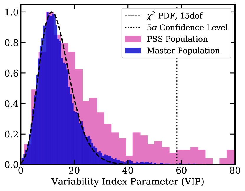
Figure 1: Histogram of the VIP as a measure of spectral variability for both the master population (blue) and the PSS population (pink) normalised to a maximum of one. The master population was modelled with a $\chi^{2}$ probability density function with 15 degrees of freedom and is consistent with a population which is mostly non-varying. Using this distribution a 99.99994% confidence level, corresponding to a VIP of 58.3, was used to determine whether a source was variable. The PSS population is not well defined by a $\chi^{2}$ distribution, implying it is likely a more intrinsically variable population.

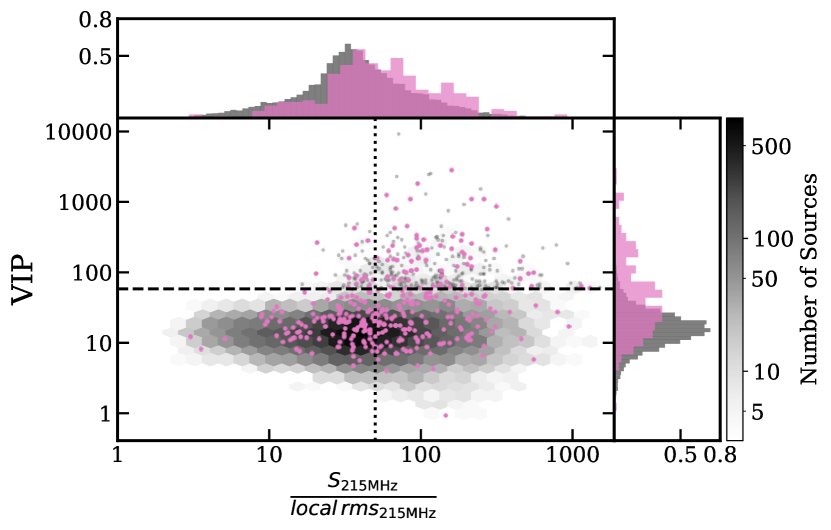
Figure 2: Distribution of the VIP as a function of the signal-to-noise ratio (S/N) in the 200–231 MHz wide band mosaic. The grey hexagons represent the density of the master population (as indicated by the colour-bar). Pink dots are sources identified as persistent PSS and grey points are all other variable sources. The dashed horizontal line is the 99.99994% VIP confidence level of 58.3 (equivalent to 5$\sigma$): sources with a VIP$\geq$58.3 are classified as variable. The distribution of the S/N for the master population and PSS population is shown in the grey and pink histograms in the top panel. The dotted vertical line denotes a S/N cut of 50 where the PSS population is complete, relative to the master population. The grey and pink histograms in the right panel represent the VIP distributions for the master population and PSS population respectively for sources with a S/N above 50. The PSS VIP histogram shows a significantly different distribution to that of the master population with a peak at higher VIP, a wider distribution, and longer tail towards higher VIP.

3.2 Measure of Spectral Shape

The large fractional bandwidth of this study enables us to detect changes in spectral shape between epochs. We classified the variable population into two classes of spectral variability:

1. Uniform change: all 16 flux density measurements increase or decrease by the same absolute amount (within uncertainty);

2. Changing shape: the shape of the spectrum has changed between epochs.

To distinguish between these two categories, we define the measure of spectral shape (MOSS) parameter. The MOSS parameter uses the flux density measurements directly to detect changes in spectral shape in order to reduce uncertainties that accompany fitting spectral models. The MOSS parameter is also a variation of the $\chi^{2}$ statistic, namely:

$$\mathrm{MOSS}=\sum^{n}_{i=1}\frac{(\widetilde{\mathrm{diff}}-\mathrm{diff}(i))^{2}}{\sigma_{i}^{2}}$$ (2)

where $\widetilde{\mathrm{diff}}$ is the median of the differences between the flux density over all frequencies, $\mathrm{diff}(i)$ is the difference of the flux densities between the two epochs at frequency $i$, and $\sigma_{i}$ is the combined uncertainty of each flux density added in quadrature. Unlike the VIP, the MOSS parameter measures how many flux density points are greater than $1\sigma$ away from the median difference value. A larger MOSS value suggests a larger spread of the difference in measurements from the median value between the two epochs and hence a change in spectral shape.

The distribution of the MOSS parameter for the non-variable population is most consistent with a $\chi^{2}$ probability density function with 12 dof, as shown in Figure 3. Hurley-Walker et al. (2017a) noted that the errors within the 30 MHz bands of GLEAM are correlated. Since we are measuring correlated change away from a central point, this has a stronger effect on the MOSS parameter than the VIP. We hypothesise that this is the cause of the reduced number of degrees of freedom of the optimal PDF distribution, given we expect 14 dof. Using the distribution of the non-variable population a value of $36.7$ and above for the MOSS parameter was chosen to select sources that are 99.99994% likely to be truly changing shape (equivalent to a 5$\sigma$ confidence level). We define the uniform change population as variable sources with no significant change in spectral shape according to the MOSS parameter (with a MOSS parameter below $36.7$). Likewise we define the changing spectral shape population as variable sources with a significant change in spectral shape according to the MOSS parameter (with a MOSS parameter $\geq 36.7$).

The spectra of two examples sources that are classified as changing spectral shape according to the MOSS parameter are presented in Figure 4.

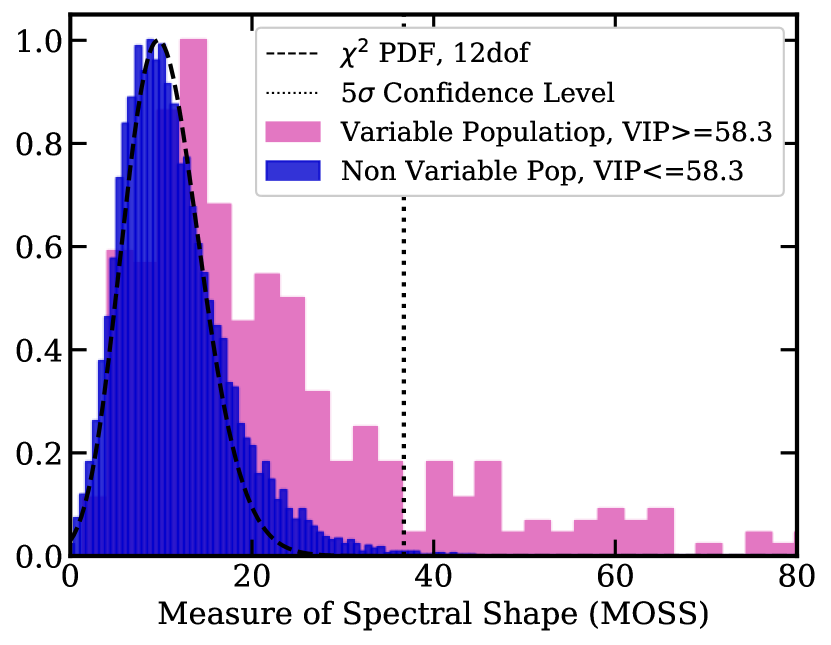
Figure 3: Histogram of the MOSS parameter, a measure of the variability of spectral shape, for the non-variable master population (blue) and the 323 variable sources (sources with a VIP$\geq 58.3$) (pink) both normalised to have the max number of sources in a bin as 1. This distribution was fit with a $\chi^{2}$ probability density function and is consistent with the majority of variable sources not displaying changing spectral shape. Using this distribution, a 99.99994% confidence level, corresponding to a MOSS parameter $>36.7$, was used to determine a significant change in spectral shape between Year 1 and Year 2.

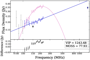
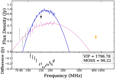
Figure 4: Examples of radio spectra of two variable sources showing a significant change in spectral shape between Years 1 and 2. One was found to be have a peaked spectrum in Year 1 and then flattened in Year 2 (GLEAM J225641–201140, left panel) and the other (GLEAM J032237–482010, right panel) showed the reverse. The points represent the following data: GLEAM low frequency (72–100 MHz) (grey circles), Year 1 (pink circles), Year 2 (blue circles), TGSS (black square), SUMSS (yellow pentagon), and NVSS (navy diamond). The difference of the flux densities in Year 1 and 2 are plotted below. Models plotted for each year are determined by the PSS classification only. A source classified with a peak within the observed MWA band, which also satisfied the PSS criteria presented by Callingham et al. (2017), was modelled by a quadratic according to Equation 4. Remaining sources were modelled by a power-law according to Equation 3, see Section 3.3 for details.

We note that the MOSS parameter could potentially miss truly changing spectral shape sources if the difference between the two epochs are symmetric around the mean frequency. For example, GLEAM J234312–480659 (Figure 5) shows a “tick” shape in its difference spectra. Therefore, it is classified as uniform change rather than changing shape. Furthermore, it is harder to detect a change in spectral shape for sources with lower S/N. After careful testing to balance a reliable changing shape population with completeness, sources with a MOSS $>36.7$ are classified as changing spectral shape, corresponding to a confidence level of 5$\sigma$.

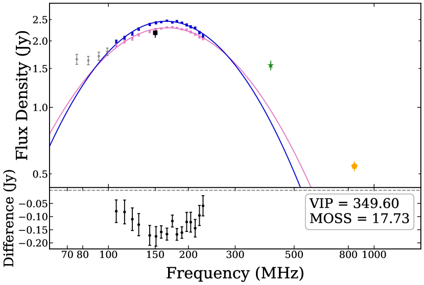
Figure 5: Example of a source for which there is insignificant change in spectral shape according to the MOSS parameter 5$\sigma$ confidence level cut despite the sharper peak in the spectra for Year 2. The data points represent the following data: GLEAM low frequency (72–100 MHz) (grey circles), Year 1 (pink circles), Year 2 (blue circles), TIFR GMRT 150 MHz Sky Survey Alternative Data Release 1 (TGSS) (black square), MRC (green star), and SUMSS (yellow pentagon). Residuals are calculated by differencing the flux density measurements of the two epochs of observations. The models for each year are determined by the classification of the source; We identify a peak within the observed bandwidth that is well modelled by a quadratic according to Equation 4 for both years.

3.3 Spectral Modelling

Following the spectral modelling outlined by Callingham et al. (2017), the flux density measurements for each source for both years were fit with two different models using the non-linear least squares python scipy module, curve_fit (Virtanen et al., 2019):

1. Power-law: A model that fits the flux density distribution of sources whose emission is primarily non-thermal:

   $$S_{\nu}=a\nu^{\alpha},$$ (3)

   where $S_{\nu}$ is the flux density at frequency $\nu$ and $a$ is the amplitude of the spectrum. This model was fit to two datasets: (1) the 16-band MWA data (100–231 MHz) to measure the spectral index for the low frequency section of the SED, $\alpha_{\mathrm{low}}$, and; (2) two MWA flux density measurements (189 and 212 MHz) and the flux density of the SUMSS and/or NVSS counterpart to measure the spectral index for the high frequency section of the SED, $\alpha_{\mathrm{high}}$.

2. Quadratic: A non-physical model to detect any spectral curvature within the MWA band. This is only fit to the 16-band MWA data (100–231 MHz):

   $$S_{\nu}=a\nu^{\alpha}\exp^{q\left(\ln\nu\right)^{2}},$$ (4)

where $q$ represents the spectral curvature and the other parameters are as defined in Equation 3.

It is worth noting, when classifying PSS using observations at different frequencies taken at different times, it is possible to over-estimate or under-estimate the spectral indices due to variation in fluxes (e.g. due to scintillation or Doppler boosting at higher frequencies, i.e. the peak may seem more pronounced when combining different epochs of observation). Consequently, the best way to detect and classify PSS is with simultaneous megahertz and gigahertz-frequency spectral coverage of the SED with monitoring of a least a year to determine if the source maintains its PSS classification. In common with all other searches in the literature so far, our PSS classifications rely on measurements taken over different epochs (i.e. SUMSS/NVSS), implying there will be false positives in the population.

4 Results

Firstly, we compare the distributions of $\alpha_{\mathrm{low}}$, $\alpha_{\mathrm{high}}$ and $q$ with those presented by Callingham et al. (2017). In both the Year 1 and 2 data, the majority of sources lie close to a $\alpha_{\mathrm{high}}=\alpha_{\mathrm{low}}$ line, consistent with no change of spectral index across the full frequency. The median and standard deviation for $\alpha_{\mathrm{low}}$ and $\alpha_{\mathrm{high}}$ are $-0.82\pm 0.28$ and $-0.76\pm 0.24$ in Year 1, and $-0.81\pm 0.28$ and $-0.76\pm 0.22$ in Year 2.

The curvature parameter distributions for Year 1 and Year 2 are both consistent with those found by Callingham et al. (2017) with the median curvature, $q$, and standard deviation for Year 1 and Year 2 found to be $-0.12\pm 0.50$ and $-0.12\pm 0.41$ respectively. We compared distributions for $\alpha_{\mathrm{low}}$, $\alpha_{\mathrm{high}}$ and $q$ with those presented by Callingham et al. (2017) and find no significant differences.

From the 21,558 sources of the master population, we have identified 323 sources that have VIP$\geq 58.3$ and classified them as variable. The majority of sources in this variable population show no significant change in spectral shape between the two MWA epochs, with 272 sources ($\sim$84 per cent) showing a uniform spectral change across the observed bandwidth. The other 51 sources ($\sim$16 per cent) are classified as changing spectral shape, since their spectral shapes change significantly from Year 1 to Year 2 as their MOSS parameter was $\geq 36.7$.

Of the variable population, 91 sources ($\sim 28\%$) were identified as PSS by Callingham et al. (2017). We also classified sources in the master population as PSS according to the same criteria outlined by Callingham et al. (2017), and find 123 sources identified as PSS in either year in the variable population ($\sim$38 per cent). We find 83 PSS in the variable population maintain a PSS classification in both years (67 per cent of sources identified as PSS in either year).

One variable source, GLEAM J043715–471506, shows extreme variability (with a VIP of 9,124); see Figure 1 in Appendix B for the SED. GLEAM J043715–471506 is a known pulsar, PSR J0437–47. Other known pulsars in the field are not included in the master population as they fail to meet the brightness cut, see step 2 in Table 2.

We identify six sources – GLEAM J001942–303118, GLEAM J010626–271803, GLEAM J033112–430208, GLEAM J033412–400823, GLEAM J041636–185102, GLEAM J215155-302751 – which were classified as potential restarted galaxies by Callingham et al. (2017) due to their “upturned” SEDs, each with a VIP$\geq 64$. We conclude that these sources were misclassified and are likely not restarted galaxies but variable quasars with flat spectra. Of the 25 sources identified as “upturned” SEDs by Callingham et al. (2017), 19 sources (76 per cent) are not identified as variable.

Mid infra-red colour selection techniques using Wide-field Infrared Survey Explorer (WISE, Wright et al., 2010) are widely used to distinguish between AGN and star-forming galaxies (e.g., Lacy et al., 2004; Stern et al., 2005; Wu et al., 2012; Assef et al., 2013). We compare our variable population with the WISE infra-red colours and find all variable sources are consistent with AGN/quasar classifications, as expected based on the flux density limit of our sample. Furthermore, we searched for any trend in VIP or MOSS with Galactic latitude and find none.

4.0.1 Variable Persistent PSS Population

Of the persistent PSS in the variable population, 11 sources ($\sim$13%) are classified as showing a change in spectral shape between epochs according to the MOSS parameter, while still maintaining a PSS classification. For example, some persistent PSS may have a positive spectral index, $\alpha_{\mathrm{low}}$, in each year but the steepness changes significantly according to the MOSS parameter. The other 72 sources are classified as showing a uniform change across the MWA bandwidth.

There are four sources that are classified as variable persistent PSS but are not classified as PSS by Callingham et al. (2017). The inconsistency in classification is likely due to the lack of the lowest band in this study, which prevented a robust fit in the optically thick region of the SED, making their peaked-spectrum classification less certain. These four sources are GLEAM J020903–495243, GLEAM J041913–142024, GLEAM J042140–152734 and GLEAM J234625–073042.

4.0.2 Changing Spectral Shape

We detect 51 variable sources that have a MOSS parameter $>36.7$, and are thus classified as showing a significant change in their spectral shape between epochs. Of these changing spectral shape sources, 18 (20 per cent) were selected as PSS by Callingham et al. (2017). The significant change in spectral shape suggests even if these sources maintain PSS classification in Year 1 and 2, it is possible this is only temporary and they will lose their peaked-spectrum classification over time.

A change in spectral shape may allow more accurate identification of the astrophysics of sources. For instance, GLEAM J033023–074052 was classified peaked-spectrum by Callingham et al. (2017) but is classified as changing spectral shape between epochs. VLBI observations of GLEAM J033023–074052 found it was unresolved on milliarcssecond-scales, and constrained its projected linear size to be $<45$ pc (Keim et al., 2019). After reexamination of the optical spectral for GLEAM J033023–074052, we find the MgII line was a misidentified Lyman-$\alpha$ line (Wolf et al., 2018; Onken et al., 2019), thus the redshift is likely 2.85 rather than 0.67 as previously reported by the 6df Galaxy Survey (Jones et al., 2009) and used by Keim et al. (2019). Using the updated redshift, we recalculated the upper limit for the projected linear size of J033023–074052, and the limit increases to $<50$ pc.

The compact linear size and changing spectral shape over a year-long period is consistent with the jets from the AGN being oriented towards the observer (i.e. a blazar), as opposed to a small double source that would be expected for a young AGN. The radio SED for GLEAM J033023–074052 is shown in Figure 6.

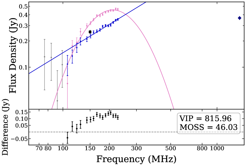
Figure 6: GLEAM J033023–074052, classified as changing spectral shape in this paper according to the MOSS. This source has also been found to be unresolved with VLBI with an upper limit on the projected linear size of 50 pc (from the new redshift presented here and the angular size reported in Keim et al., 2019). The points represent the following data: GLEAM low frequency (72–100 MHz) (grey circles), Year 1 (pink circles), Year 2 (blue circles), TGSS (black square), and NVSS (navy diamond). In Year 1 the spectrum is classified with a peak within the observed band and was modelled by a quadratic according to Equation 4, and the Year 2 spectrum was modelled by a power-law according to Equation 3.

4.1 AT20G Counterparts

Murphy et al. (2010) present a blind search for radio sources using the Australia Telescope Compact Array (ATCA) at 20 GHz. At 20 GHz, the brightness of radio galaxies is more likely to be core-dominated. We cross-matched our master population with the AT20G survey to identify sources that are dominated by their core flux density and/or are more likely to be blazars. Of the 1020 sources in our master population that have a counterpart in AT20G, 116 sources are classified as variable (11 per cent).

This result contrasts with just $\sim$1.6% of the total master population being variable and therefore supports the idea that core-dominated radio sources are more likely to be variable. Furthermore, of the variable sources with AT20G counterparts, we identify 24 sources (21 per cent) as changing spectral shape, larger than the 16 per cent of the total variable population showing significant change in spectral shape.

We note one source in particular, GLEAM J032237–482010, has a significant change in spectral shape (MOSS$\approx$90) yet has no AT20G counterpart. GLEAM J032237–482010 does have a flux density of $\sim 0.5$ Jy at 840 MHz according to SUMSS. If GLEAM J032237–482010 is a quasar with a flat spectrum around 0.5 Jy or a blazar with a temporary peak in the SED, the core should be bright enough for an AT20G detection. The non-detection of AT20G suggests this source is not core dominated, contradictory to what the variability suggests. The SED for GLEAM J032237–482010 is presented in Figure 4.

4.2 Known blazars in the variable population

Massaro et al. (2015) combined optical spectra and absorption lines with the radio spectra to identify blazars, which they present in the Roma-BZCAT catalogue. We cross-match our master population with Roma-BZCAT and find 295 sources with a BZCAT counterpart. Of these sources, 64 are classified as variable by the VIP (22 per cent), 18 of which (28 per cent) are classified as changing spectral shape according to the MOSS parameter. This is a larger proportion of sources classified as changing spectral shape compared to the total variable population of which the changing spectral shape sources make up 16 per cent.

4.3 Comparison to literature 150 MHz variability studies

4.3.1 MWA Transients Survey

The MWA Transients Survey (Bell et al., 2019, MWATS;) was a blind search for variable sources at 150 MHz over 3–4 years. We compare our variable population with the sources identified by the single frequency variability identified by MWATS and find no overlap. Of the 15 variable sources identified by MWATS, seven were in our field and no source had a VIP$\geq$23.

By considering the light curves presented by Bell et al. (2019) for the seven sources in our field, it appears MWATS is more sensitive to changes in flux density over 3–4 years, while this work considers only two epochs one year apart. The different parameter spaces each survey explores suggest different astrophysical explanations are driving the observed variability. MWATS predominantly attributes their observed variability to RISS. We explore the viability of RISS as the cause for the observed variability of this survey in Section 5.1.

4.3.2 Interplanetary Scintillation with the MWA

We performed a cross-match of the master population with the catalogue of sources displaying IPS from Chhetri et al. (2018) and found 1,873 sources in our field, only 40 of which had a VIP$\geq 58.3$. Of the variable sources presented in the IPS catalogue, only four are reported as non-scintillating while 28 are reported as highly scintillating with a normalised scintillation index above 0.9. We note, Chhetri et al. (2018) report 12 per cent of their total population were strongly scintillating due to IPS while 90 per cent of the variable sources in the field are at least moderately scintillating.

Chhetri et al. (2018) identify 37 compact sources according to IPS and search for variability at 150 MHz within this sample. The one source identified as variable, GLEAM J013243–165444, is also in our master population. We also classify GLEAM J013243–165444 as variable source with significant change in spectral shape with a VIP of $\sim 122$ and a MOSS parameter of $\sim 85$. Despite its blazar identification and variability in both surveys, GLEAM J013243–165444 maintains a peaked spectrum in both years of GLEAM observations with a peak at $\sim$150 MHz. There are several sources within the changing spectral shape population that temporarily display a peaked-spectrum classification. Such temporary spectral peaks have also been identified by Torniainen et al. (2005). It is thus possible that the PSS classification of GLEAM J013243–165444 is also temporary. The SED for GLEAM J013243–165444 is presented in Figure 1 in Appendix B.

4.4 GMRT Search for Transients

The VIP is calculated using only two epochs but takes advantage of the 16 individual flux density measurements. Hajela et al. (2019) present a statistical method which compares two epochs on over four different timescales (4 hours, 1 day, 1 month and 4 years) but only uses one flux density measurement for each epoch. We apply the methodology presented by Hajela et al. (2019) to our master population to probe variability over one year at a single frequency, and compare this to the VIP. Such a comparison helps us put our methodology of identifying variability in the context of the literature.

We calculate their variability statistic, $V_{s}$, at 150 MHz:

$$V_{s}=\frac{\left(S_{1}-S_{2}\right)}{\sqrt{\sigma_{1}^{2}+\sigma_{2}^{2}}},$$ (5)

and the modulation index, $m$:

$$m=2\times\frac{S_{1}-S_{2}}{S_{1}+S_{2}},$$ (6)

where $S_{1}$ and $S_{2}$ are the flux densities in the first and second epoch, respectively. $\sigma_{1}$ and $\sigma_{2}$ are the uncertainties on the measurements. Hajela et al. (2019) state a source is truly variable if the $V_{s}$ is more than four times the standard deviation of $V_{s}$ and $|m|>0.26$. Using this classification of variability on our MWA master sample at the 150 MHz, we find 13 sources which would be what Hajela et al. (2019) define as truly variable. Of these 13 sources, 12 are selected by the VIP as showing significant variability as shown in Figure 7, all of which have a VIP$\geq$85. Additionally, of these 13 sources, only two are classified as having a change in shape, and 11 are classified as having a uniform change across the band. The VIP takes full advantage of the multiple flux density measurements and is thus more robust to single frequency random fluctuations. The $V_{s}$ and $m$ presented by Hajela et al. (2019) has a high reliability, but a low completeness, missing a large fraction of variable sources at low frequencies, shown by black dots in Figure 7.

Separately, we cross-match our variable population with that presented by Hajela et al. (2019) and find only one common source. GLEAM J012528–000557 (referred to as J012528+000505 in Hajela et al., 2019), is found to be variable in this work and by Hajela et al. (2019). This source is a known blazar (Section 4.2) and thus variability at these frequencies on timescales of years is not unexpected.

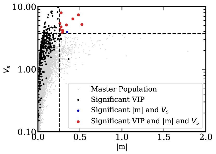
Figure 7: The distribution of the variability statistics defined by Hajela et al. (2019) for our master sample; the y-axis shows $V_{s}$ (Equation 5), as a function of the modulus of the modulation index, $m$ at 150 MHz (Equation 6). The different populations are listed in the legend. Many sources that are variable according to the VIP are missed by the $V_{s}$ and $m$. Using single-frequency variability statistics seems to cause low completeness.

5 Discussion

As we have classified the observed variability according to the type of variability observed, and compared it to other low-frequency variability studies, we now discuss the potential physical mechanisms that could drive each variability classification.

5.1 Extrinsic Variability

Scintillation can cause radio sources to vary in brightness over several different timescales depending on the scattering regime. The mosaics used in this study are composed of multiple 2 minute snapshots, and IPS and ionosphere scintillation timescales are short enough that the variations will be smoothed over in the mosaics. Likewise the high Galactic latitude of our survey area places the transition frequency from weak scattering to the strong scattering at $\gtrsim 1$ GHz. Therefore, variability identified in our survey is probing the strong scattering regime (Walker, 1998).

Refractive interstellar scintillation (RISS) in the strong regime can cause variability at megahertz frequencies on year-long timescales. In comparison, diffractive interstellar scintillation (DISS) occurs on shorter timescales (seconds to minutes) and with a larger amplitude of modulation (Narayan, 1992). Furthermore, DISS requires much smaller limits on source size than RISS, so more strongly influences light from extremely compact sources such as pulsars and fast radio bursts, and is a narrow band effect (with the fractional decorrelation bandwidth $\ll 1$ Narayan, 1992). We thus attribute the observed variability of the known pulsar GLEAM J043715–471506 (PSR J0437-47) to DISS, further supported by the irregularity of the SED suggesting significant frequency dependence on the modulation within the MWA bandwidth. We focus on RISS in the following sections when considering scintillation as the cause for the observed variability.

Extended sources can still scintillate if they have point-like components embedded within the extended structure, such as hotspots in the lobe of a radio galaxy. However, for sources with an angular size far larger than the scintillation angle, and with no such compact features, the combined modulation of the smaller regions averages to a negligible total modulation. Thus, if we assume the source is point-like and find the spectral variability consistent with scintillation, it is also consistent with a point-like structure embedded within an extended source. However, for an extended structure, the point-like region is a fraction $f$ of the total flux density. The point-like region will still scintillate while the extended structure will not. Consequently, for extended sources, we measure the modulation index reduced by a factor $1-f$, (Hancock et al., 2019). Hence, the compact region needs to dominate the emission from the lobes of a radio galaxy for scintillation to produce the observed variability. Furthermore, if the scintillating component is larger than the Fresnel angle, the scintillation timescale increases (Narayan, 1992).

We also consider the possibility that extreme scattering events (ESEs) could cause some of the observed variability (e.g. Bannister et al., 2016). While the features of some of the observed variability are consistent with an ESE, current confirmed detections of ESEs suggest they are rare events. Lazio et al. (2001) only report finding 15 events in a survey of almost 150 sources monitored roughly once every two days for up to 15 years). We thus discount ESEs as a likely explanation for the variability observed, but suggest a third epoch of observations on our sample is required to test the validity of this assertion.

We outline below the feasibility of RISS as the mechanism behind the observed variability for each class of variable source we observe. We note, however, that we have made several necessary assumptions regarding scintillation that may not be valid for all of the sources. For example, it possible the transition frequency for weak scattering by refractive scintillation may be much lower than expected. Consequently, this survey may be probing a transition space where many assumptions are no longer viable. However, given this study is at low (megahertz) frequencies and probing timescales of around a year, it is reasonable to assume we are well within the strong scattering regime since the transition frequency is $\gtrsim 1$ GHz.

5.1.1 Non-PSS Uniform Change Population

While scintillation strength is dependent on wavelength, RISS is a broadband effect at megahertz frequencies (with the fractional decorrelation bandwidth $\sim 1$; Narayan, 1992). Thus, we expect any variability due to RISS to be approximately uniform across the $\sim$100–230 MHz bandwidth of this study (Narayan, 1992; Hancock et al., 2019).

Variable sources that are classified as having a uniform spectral change may have bright embedded compact features that can scintillate within their extended radio lobes, including but not limited to knots, jets, and hot spots. For such sources where the compact scintillating feature is embedded, the timescales are longer and the amount of modulation decreases as the observed scintillation is a combined average of individual regions scintillating. Sources with spectra which change uniformly can be interpreted as being compact (or their brightness being dominated by compact components) and undergoing RISS. Using estimates of the RISS of compact sources based on distribution of H$\alpha$ within the Galaxy (Hancock et al., 2019) we confirm the observed variability of sources showing a uniform change can be explained by scintillation. Scintillation on year long timescales at megahertz frequencies requires a compact component or hot spot of size $\lesssim$5 milliarcseconds, assuming a (Galactic) scattering screen at $D=10$ kpc and Kolmogorov turbulence (Narayan, 1992; Walker, 1998). The preponderance of our detected variable sources having a AT20G counterpart implies that many of our sources likely have small, compact features in their morphology.

To provide confirmation of the possibility of RISS as the cause of the observed variability, we propose a long-term monitoring of these sources at centimetre wavelengths (where interstellar scintillation is negligible for sources with an angular size greater than tens of microarcseconds). Likewise, VLBI observations to obtain high resolution morphologies of these sources could search for a compact features small enough to scintillate. VLBI is performed at $\sim$gigahertz frequencies where different features may contribute more to the integrated flux density than at megahertz frequencies. Assumptions of how the morphology changes with respect to frequency would be necessary in order to estimate the morphology at megahertz frequencies. Alternatively, IPS at megahertz frequencies could be a way to confirm the presence of a compact component without the need for VLBI.

The morphology of the sources at different frequencies also significantly impacts the modulation due to scintillation. Megahertz frequencies are more dominated by older, likely large structures, such as radio lobes. These structures have a much larger angular size than the core or jets of an AGN. A knot or hot-spot in the lobe may not contribute as much to the overall flux density at megahertz frequencies as it does at gigahertz frequencies. Thus at low frequencies only a fraction of the flux density may be compact enough to scintillate while at higher frequencies a larger proportion (if not all) may scintillate. Long-term, multi-epoch monitoring of the entire SED paired with high resolution maps of the morphology (ideally at several frequencies) would be needed to confirm RISS as the mechanism behind the observed variability in this study. We have begun such a monitoring campaign combining roughly simultaneous observations (within a week) with the MWA and the ATCA with multiple epochs over a year long timescale.

5.1.2 Persistent PSS Uniform Change Population

As PSS are a subset of AGN, all possible explanations of variability for the non-PSS uniform change population, outlined in Section 5.1.1, are applicable to the persistent PSS uniform change population. However, we note that hot spots do not appear to be a dominant feature of PSS at gigahertz-frequencies (Keim et al., 2019). Sources larger than the source size limit of $\sim$5 mas can scintillate but have a reduced modulation index, and increased timescale of variability. If all the observed variability for the persistent PSS uniform change population is due to scintillation, at least 6% of PSS may be dominated by core-jet structures, or have a compact component in their morphology. If confirmed, the variability due to scintillation can help provide milliarcsecond resolution of structures of persistent PSS at redshifts $\gtrsim 0.5$ without the requirement of high resolution imaging using VLBI.

In order to confirm scintillation as the mechanism behind the detected variability of persistent PSS, similar follow-up campaigns for the non-PSS uniform change sources are recommended. SED coverage would need to be simultaneous (within a few days) to ensure accurate estimation of the spectral peak and spectral indices.

5.1.3 Changing Spectral Shape Population

As mentioned previously, both a point-like source and an extended source with an embedded compact feature can scintillate. In this section, we calculate the feasibility of RISS as the driving mechanism behind the observed variability for sources with a changing spectral shape.

According to Walker (1998) the modulation scales with $\left(\frac{\nu}{\nu_{0}}\right)^{\frac{17}{30}}$, where $\nu$ is the observed frequency and the transition frequency is denoted by $\nu_{0}$. We note $\nu_{0}\gtrsim 1$ GHz, thus placing this survey well into the strong regime and RISS is a broadband effect at the frequencies probed by our survey (Narayan, 1992; Walker, 1998). At megahertz frequencies and high galactic latitudes, the expected modulation is fairly constant across the 100-230 MHz band. Furthermore, if the source is scintillating, while scintillation strength does scale with frequency, the difference in the observed effect across 130 MHz bandwidth is negligible according to the decoherence bandwidth for RISS ($\delta\nu_{\mathrm{dc}}\approx 1$). Therefore, scintillation cannot be the sole explanation for those sources that show significant changes in their spectral shape.

5.2 Intrinsic Variability

The observed variability is consistent with several mechanisms of intrinsic evolutions or changes. Causes of intrinsic variability include evolution of knots in core/jet structures and changes in the immediate environment surrounding radio lobes. The megahertz frequencies of this study are probing the large scale structure and are dominated by the lobes of AGN. Hardcastle & Looney (2008) report the cores of typical AGN being four orders of magnitude fainter than the lobes at low frequencies, although it is unknown whether this holds true for compact AGN. We find it unlikely the lobes for any AGN are $\leq$1 ly ($\sim 0.3$ pc) across, which would be necessary for light travel time to explain variability on year-long timescales. We largely focus on more plausible solutions relating to interactions within the jet/lobes and nearby surrounding absorbing media:

1. Internal shocks, where shells of plasma within lobes interact and can cause a re-energisation of the electrons;

2. Knots in the jet that are being ejected from the central core and travelling to the lobes;

3. Changes in optical depth due to a fast-moving clumpy cloud of surrounding media;

4. Core or jet structures being oriented towards the observer, i.e. the possibility of all sources being blazars

As with extrinsic variability discussed in Section 5.1, we will outline the feasibility of intrinsic variability per variable class: non-PSS uniform change sources, persistent PSS, and variable spectral shape sources.

5.2.1 Non-PSS Uniform Change Population

As AGN with no detectable peak in their spectra are often significantly larger than PSS, there are some intrinsic mechanisms we can eliminate as explanations for the observed variability. For example, we can rule out variability due to the evolution of a knot travelling from the core to the lobes on a year long timescale as this is unfeasible on these timescales.

However, if the core or jet were to vary (due to changes in accretion rate, for example) we could expect to see significant changes on much shorter timescales. At low frequencies we would normally expect the lobe emission to dominate, so such variation would require either:

1. The feature varying is not travelling across the entire source: this would reduce travel time to the lobes;

2. The component of the total flux density determined by the core is greater than expected: this could result in short timescale variability from the core itself, which may be detected at low frequencies.

In the first scenario, the timescale of variability can be reduced by introducing interaction of the plasma within the jets/lobes. This interaction creates shells of energised plasma which merge and increase the lobe brightness on much shorter timescales than energy travelling from the core (Jamil et al., 2010)

Similarly in the second scenario, if the flux density is dominated by the core, we could detect the variability we observe via standard core or jet fuelling. This would suggest that for a small fraction of radio galaxies (and in particular PSS), current estimates of the relative brightness of the core to the lobes, ranging from $10^{-1}$–$10^{-4}$ (Hardcastle & Looney, 2008), is massively underestimated at low frequencies.

Furthermore, it is worth noting that 38 of the non-PSS uniform change sources are known blazars (of a total 175 non-PSS uniform change sources in the field). It is thus not unreasonable to see variability on short timescales from the core or jet which is oriented towards the observer providing an additional beaming effect (Madau et al., 1987). Any slight change of the source may be Doppler Boosted and variability on year long timescales due to the flaring or changing state of a blazar could explain the observed spectral variability of these sources. However, blazars are generally compact enough to scintillate, thus disentangling whether the observed variability is due to the intrinsic variable nature of the blazar or from scintillation in the interstellar medium is challenging. Comprehensive monitoring with high time resolution of both low frequency (radio) with high frequency (X-ray and/or Gamma) follow up is required, or VLBI observations tracing the evolution of the jet.

5.2.2 Persistent PSS Uniform Change Population

Given PSS are a sub-population of typical AGN, all mechanisms explained in Section 5.2.1 are also plausible for the PSS population. But there are potentially unique intrinsic mechanisms due to the typically more compact morphologies of PSS and their interactions with the warm ISM (Bicknell et al., 2018a).

Firstly, a subset of PSSs may have a core-jet prominence more typically associated with AGN that have a flat spectrum, even at megahertz frequencies. As such, this core variability may arise from changes in accretion rate or flaring state. If we assume an impulsive change at the core to be the cause of the variability, we would expect a uniform decrease across the entire SED of the source if the material is adiabatically expanding. In this case, the cause of the overall persistent peak in the SED remains the same. As outlined in Section 5.2.1, current estimates of the core prominence place core flux density at $10^{-1}$–$10^{-4}$ times fainter than the lobes at low frequencies ($\sim$150 MHz) for typical AGN. However, measurements of the core dominance for PSS have yet to be reliably measured at megahertz-frequencies. Furthermore, for the PSS that have a compact double morphology, the core is hardly ever even detected (Orienti, 2016). Thus, the identified variable PSS in this study may have an inherently different core prominence. If a multi-epoch follow up with simultaneous observations of the broad band SED ($\sim 70$ MHz–$\geq 10$ GHz) showed a flare typical of a changing state in the core and/or jet, we could surmise a larger component of the flux density measured at megahertz frequencies is due to the core. Intrinsic variability due to the core may signify persistent PSS have a vastly different core prominence than their non-peaked counterparts. Only LOFAR will have the resolution in the coming decades to potentially resolve some of these sources at megahertz-frequencies.

Secondly, similar temporary peaks in radio spectra have been observed in X-ray binary systems where ejecta from the jet has been observed (Fender et al., 2009; Tetarenko et al., 2019). Radio monitoring for Cygnus X-1 detected a lag of the radio flare from higher radio frequency to lower radio frequency (11 GHz down to 2 GHz Tetarenko et al., 2019). Furthermore, Tetarenko et al. (2019) report a decreased amplitude of modulation and increased width of the timescale of the flare at lower frequencies ($\sim 2$–3 GHz). Tetarenko et al. (2019) suggest this delay is due to the different frequencies probing further along the jet away from the core, with higher frequency observations probing younger, faster-evolving material. While black hole X-ray binary systems are orders of magnitude more compact than AGN, varying on the timescales of weeks, a similar mechanism could explain the observed variability of the persistent PSS but on year long timescales, given the typically compact ($\leq$20 kpc) morphology of PSS. Observing the light curves at multiple radio frequencies over year long timescales for the persistent PSS may show a delay in the flare from higher frequencies to lower as the ejection from the jet travels further from the core. Furthermore, given it is not unreasonable to expect ejecta from the jets being detected on these timescales for PSS, it is also justifiable to explain the observed variability with interacting shells (Jamil et al., 2010), which theoretically occur on shorter timescales.

Thirdly, one potential cause of the variability below the spectral turnover could be due to changes in the free-free optical depth along the line of sight (e.g. Tingay et al., 2015). The free-free absorption (FFA) model has been considered as the cause of absorption in the optically thick region for at least some PSS (Peck et al., 1999; Kameno et al., 2000; Tremblay et al., 2008; Marr et al., 2014; Callingham et al., 2015; Tingay et al., 2015). Attributing the variability to changes in optical depth would be evidence to support the FFA model for these sources. Recent simulations have also proposed GPS and CSS are the result of relativistic jet feedback and interactions with the surrounding warm ISM (Bicknell et al., 2018b). Several observations of absorption features linked with dust surrounding AGN have also found a strong connection with PSS (Grasha et al., 2019; Glowacki et al., 2019; Jarvis et al., 2019). However, as several studies have noted (O’Dea, 1998; Callingham et al., 2017; Bicknell et al., 2018a), distinguishing between synchrotron self absorption (SSA) and FFA for the PSS population as a whole has thus far yielded inconclusive results as both SSA and FFA spectral models are consistent with current observations for most PSSs. Testing for prominent HI gas via would help identify galaxies that likely have a lot of intervening media between us and the radio lobes (Callingham et al., 2015).

We note it is entirely possible that the majority of the persistent PSS population may be entirely composed of flaring blazars that are observed at both epochs with a peaked spectrum. While only 25 per cent of the persistent PSS population were known blazars, as selected based on X-ray, optical and gigahertz-frequency characteristics, it is possible other members of the persistent PSS population happen to have a jet orientation relative to our line-of-sight that ensures it is not X-ray- or optically-bright relative to its radio luminosity. Blazars are also known to display a peaked spectrum over a prolonged period, even at gigahertz-frequencies (Chhetri et al., 2018). For example, we find known blazar GLEAM J013243–165444 to be classified as a PSS in both years of observation. We thus suggest long-term observations of the light curves of the persistent PSS population at either gigahertz frequencies or, if the sources are bright enough, follow up with $\gamma$- or X–ray telescopes, like the extended ROentgen Survey with an Imaging Telescope Array (eROSITA; Predehl et al., 2016). Furthermore, follow up with multi-frequency VLBI would be critical to determine if these sources are core-jet or double-lobed objects.

5.2.3 Changing Spectral Shape Population

For intrinsic variability of a source emitting synchrotron radiation, the brightness temperature ($T_{b}$) has an upper limit of $10^{12}$ K, as determined by the inverse-Compton losses. We reproduce the calculation used by Bell et al. (2019) to estimate if changes in the flux density are within expectations for intrinsic variability using the following equation:

$$\Delta S\leq\frac{2k_{B}\nu^{2}\tau^{2}T_{b}b^{3}}{D^{2}},$$ (7)

where $\Delta S$ is the change in flux density, $\tau$ is the timescale (here 1 yr), $T_{b}$ is the brightness temperature (set as the upper limit, $10^{12}$ K), $b^{3}$ is a beaming factor for emission directed towards the observer (we assumed an upper limit of 10, a typical value for blazars (Lahteenmaki & Valtaoja, 1999)), and $D$ is the distance to the source (set as 10 Gpc, equivalent to roughly $z=1$). Using Equation 7 we find that sources can not exceed 0.68 Jy for $\Delta S$ at 150 MHz when no beaming factor is used. By introducing the beaming factor for incoherent emission, all the observed variability for these sources can be explained via intrinsic mechanisms. We thus suggest that sources where we observe a variable spectral shape between epochs as beamed AGN. 24 of the 51 (47 per cent) changing spectral shape sources have AT20G counterparts (Murphy et al., 2010), suggesting core-dominance. Additionally, 18 sources (35 per cent) are known blazars already from BZCAT (Massaro et al., 2015).

However, it is worth noting that if these sources are indeed heavily beamed, their morphology will likely be compact enough that they may also scintillate. Therefore, it is possible the observed variability is a combination of both intrinsic blazar flares and scintillation. Finally, we note that we assumed a timescale of one year due to the rough timescale of this work in searching for variability but it is likely these sources have variability that will occur on longer timescale than observed. Increasing the timescale of variability increases the $\Delta S$ limit, according to Equation 7, for these sources to be intrinsically variable. Thus, further long-term monitoring over several years with wide spectral coverage is necessary to estimate the true timescale more accurately as well as determine the role of scintillation.

If confirmed, spectral shape variability at low frequencies ($<1$ GHz) has the ability to detect and classify blazars on relatively short timescales, even if they are too faint to observe at higher frequencies.

5.3 Summary of plausible causes of the observed variability

Considering causes for intrinsic or extrinsic variability, we determined the most likely causes for the observed spectral variability for the different classes of sources. For non-PSS and PSS sources that show a uniform change in their SED between epochs, scintillation can easily explain the observed low-frequency variability. If confirmed, observing the variability due to scintillation could be paired with observations of pulsars to increase the resolution of maps of the electron column density to test models that aim to predict scintillation, such as RISS19. In contrast, the sources in which we observe a changing spectral shape between epochs are more likely explained as a blazar with changing flaring states. While scintillation may be a component of the observed variability it is unlikely the sole mechanism to explain the spectral shape variability due to the wide bandwidth of RISS. We therefore present the changing spectral shape variable population as blazar candidates requiring a follow-up campaign for confirmation, for example a search for X-ray counterparts with eROSITA (Predehl et al., 2016).

6 Conclusions and Outlook

We have conducted a study of low-frequency spectral variability and devised a methodology for detecting, measuring, and classifying spectral variability using the variability index parameter (VIP) and the measure of spectral shape (MOSS) parameter. This study uses two epochs of the GLEAM survey, producing a data set that contains over 21,000 sources. Therefore, our study represents the largest survey of low-frequency spectral variability, particularly of spectra formed from contemporaneous flux density measurements over a large fractional bandwidth.

We present 323 sources that show significant spectral variability according to the VIP, 51 of which display a significant change in shape of their spectra according to the MOSS parameter. We find that the variable sources are more likely to have a peaked spectrum, consistent with results from the MWATS and IPS surveys with the MWA. We compare the variable population with the WISE infrared survey to determine the classification of galaxy and find no variable sources to be classified as star forming. Furthermore, we conclude many of the variable sources are consistent with quasar and blazar classifications. We also compare the variable population with BZCAT to find known blazars. There is a larger proportion of variable sources that are known blazars (22 per cent) compared to the master population ($\sim$1 per cent), with many of the remaining variable population possessing characteristics similar to the identified blazars. Likewise, we find a larger proportion of variable sources with AT20G counterparts (11 per cent) when compared to the master population (1 per cent). One source in particular, GLEAM J 032237–482010, shows a significant change in spectral shape, suggesting it is a core-dominated source or a blazar, yet has no AT20G counterpart.

We discuss several sources that have particular interesting features. For reported restarted radio galaxy candidates, we find that six are variable and conclude they are misclassified quasars with a flat spectra. We compare our variable sources with several notable single frequency variability surveys conducted around 150 MHz and only find two sources which are classified as variable in each, both of which are known blazars: GLEAM J012528–000557 and GLEAM J013243-165444. We also find one known pulsar, PSR J0437–47, to show significant variability and conclude this is likely due to diffractive interstellar scintillation.

We argue that the observed variability of the persistent PSS and uniform change sources are entirely consistent with refractive interstellar scintillation. The sources which show a changing spectral shape according to the MOSS parameter cannot be explained by ISS and we thus present this population as blazar candidates requiring further confirmation.

While we suggest likely causes for each category of spectral variability, it is worth noting this is based on only two epochs of observation. Long term monitoring and specific follow up campaigns are recommended to test the presented hypotheses. Furthermore, in all cases having more epochs of observation with greater spectral coverage from megahertz to gigahertz frequencies would increase the reliability of detected variability. Thus a lower level of significance cut off for the VIP could be used to detect variability. More epochs of observation on a range of timescales could allow for the timescale of variability to be accurately estimated, this can refine viable variability mechanisms.

6.1 SKA Era Implications

In the SKA era, as we gain the capability to perform large scale variability surveys with large spectral and temporal coverage, understanding how prevalent variability is at low frequencies is crucial. This paper outlines a methodology to begin dissecting this variability by detecting and classifying the low-frequency spectral variability with rigorous and reproducible statistical methods. MWATS place an upper limit prediction on the expected number of variable source at low frequencies ($\sim$150 MHz) of 6,000 sources for a given sample of 350,000 sources. Following this trend, we would expect fewer than 400 variable sources in this study. Our results are consistent with this expectation numerically, however, the nature of spectral variability detected suggests our current understanding of low-frequency variability is not yet complete. These results highlight the insufficient understanding of the emission mechanisms at low frequencies, and AGN evolutionary scenarios. As many PSS are used for calibrators of high-frequency (gigahertz) radio telescopes, understanding the short-timescale ($\sim$years) evolution and variability of their SEDs is critical. Despite this variability being observed at low frequencies, it is important to see how this variability relates to the gigahertz regime. Furthermore, SKA_LOW will be able to detect fainter PSS. An understanding of the current known PSS population is critical if we are to investigate the fainter population. We encourage careful monitoring of the presented sources in this paper in order to understand how they may change within the span of future surveys and studies.

7 Data Availability

The data underlying this article are available in the article and in its online supplementary materia

Appendix A Supplementary Online Catalogue Description

Column numbers, names, units and description for the supplementary online catalogue. Source names follow International Astronomical Union naming conventions for co-ordinate-based naming. Background and RMS measurements were performed by BANE; the fitted spectral index parameters were derived as described in Section 3.3; other measurements were made using Aegean or measurements from additional surveys, as mentioned in Section 2.4. Aegean incorporates a constrained fitting algorithm. The columns with the subscript “wide” are derived from the 200–230 MHz wide-band image. Subsequently, the subscript indicates the central frequency of the measurement, in MHz. These sub-band measurements are made using the priorised fitting mode of Aegean, where the position and shape of the source are determined from the year 2 wide-band image, and only the flux density is fitted.

Number	Name	Unit	Description
1	GLEAM Name	hh:mm:ss+dd:mm:ss	Name of the source in the GLEAM extragalactic catalogue
2	RA_hms	hh:mm:ss	Right ascension
3	Dec_dms	dd:mm:ss	Declination
4	RA	∘	Right ascension
5	err_ra	∘	Error on RA
6	Dec	∘	Declination
7	err_dec	∘	Error on Dec
8	int_flux_wide_yr1	Jy	Integrated flux density in year 1 wideband image
9	err_int_flux_wide_yr1	Jy	Error on integrated flux density in year 1 wideband image
10	local_rms_wide_yr1	Jy beam-1	Local RMS in year 1 wideband image
11	a_wide_yr1	$\arcsec$	Major axis of source in year 1 wideband image
12	b_wide_yr1	$\arcsec$	Minor axis of source in year 1 wideband image
13	psf_a_wide_yr1	∘	Major axis of PSF at location of source in year 1 wideband image
14	psf_b_wide_yr1	∘	Minor axis of PSF at location of source in year 1 wideband image
15	int_flux_wide_yr2	Jy	Integrated flux density in year 2 wideband image
16	err_int_flux_wide_yr2	Jy	Error on integrated flux density in year 2 wideband image
17	local_rms_wide_yr2	Jy beam-1	Local RMS in year 2 wideband image
18	a_wide_yr2	$\arcsec$	Major axis of source in year 2 wideband image
19	b_wide_yr2	$\arcsec$	Minor axis of source in year 2 wideband image
20	psf_a_wide_yr2	∘	Major axis of PSF at location of source in year 2 wideband image
21	psf_b_wide_yr2	∘	Minor axis of PSF at location of source in year 2 wideband image
22	local_rms_107_yr1	Jy beam-1	Year 1 local RMS at 107 MHz
23	S_107_yr1	Jy	Year 1 integrated flux density at 107 MHz
24	S_107_err_yr1	Jy	Year 1 fitting error on integrated flux density at 107 MHz
25	local_rms_115_yr1	Jy beam-1	Year 1 local RMS at 115 MHz
26	S_115_yr1	Jy	Year 1 integrated flux density at 115 MHz
27	S_115_err_yr1	Jy	Year 1 fitting error on integrated flux density at 115 MHz
28	local_rms_122_yr1	Jy beam-1	Year 1 local RMS at 122 MHz
29	S_122_yr1	Jy	Year 1 integrated flux density at 122 MHz
30	S_122_err_yr1	Jy	Year 1 fitting error on integrated flux density at 122 MHz
31	local_rms_130_yr1	Jy beam-1	Year 1 local RMS at 130 MHz
32	S_130_yr1	Jy	Year 1 integrated flux density at 130 MHz
33	S_130_err_yr1	Jy	Year 1 fitting error on integrated flux density at 130 MHz
34	local_rms_143_yr1	Jy beam-1	Year 1 local RMS at 143 MHz
35	S_143_yr1	Jy	Year 1 integrated flux density at 143 MHz
36	S_143_err_yr1	Jy	Year 1 fitting error on integrated flux density at 143 MHz
37	local_rms_151_yr1	Jy beam-1	Year 1 local RMS at 151 MHz
38	S_151_yr1	Jy	Year 1 integrated flux density at 151 MHz
39	S_151_err_yr1	Jy	Year 1 fitting error on integrated flux density at 151 MHz
40	local_rms_158_yr1	Jy beam-1	Year 1 local RMS at 158 MHz
41	S_158_yr1	Jy	Year 1 integrated flux density at 158 MHz
42	S_158_err_yr1	Jy	Year 1 fitting error on integrated flux density at 158 MHz
43	local_rms_166_yr1	Jy beam-1	Year 1 local RMS at 166 MHz
44	S_166_yr1	Jy	Year 1 integrated flux density at 166 MHz
45	S_166_err_yr1	Jy	Year 1 fitting error on integrated flux density at 166 MHz
46	local_rms_174_yr1	Jy beam-1	Year 1 local RMS at 174 MHz
47	S_174_yr1	Jy	Year 1 integrated flux density at 174 MHz
48	S_174_err_yr1	Jy	Year 1 fitting error on integrated flux density at 174 MHz
49	local_rms_181_yr1	Jy beam-1	Year 1 local RMS at 181 MHz
50	S_181_yr1	Jy	Year 1 integrated flux density at 181 MHz
51	S_181_err_yr1	Jy	Year 1 fitting error on integrated flux density at 181 MHz
52	local_rms_189_yr1	Jy beam-1	Year 1 local RMS at 189 MHz
53	S_189_yr1	Jy	Year 1 integrated flux density at 189 MHz
54	S_189_err_yr1	Jy	Year 1 fitting error on integrated flux density at 189 MHz
55	local_rms_197_yr1	Jy beam-1	Year 1 local RMS at 197 MHz
56	S_197_yr1	Jy	Year 1 integrated flux density at 197 MHz
57	S_197_err_yr1	Jy	Year 1 fitting error on integrated flux density at 197 MHz
58	local_rms_204_yr1	Jy beam-1	Year 1 local RMS at 204 MHz
59	S_204_yr1	Jy	Year 1 integrated flux density at 204 MHz
60	S_204_err_yr1	Jy	Year 1 fitting error on integrated flux density at 204 MHz
61	local_rms_212_yr1	Jy beam-1	Year 1 local RMS at 212 MHz
62	S_212_yr1	Jy	Year 1 integrated flux density at 212 MHz
63	S_212_err_yr1	Jy	Year 1 fitting error on integrated flux density at 212 MHz
64	local_rms_220_yr1	Jy beam-1	Year 1 local RMS at 220 MHz
65	S_220_yr1	Jy	Year 1 integrated flux density at 220 MHz
66	S_220_err_yr1	Jy	Year 1 fitting error on integrated flux density at 220 MHz
67	local_rms_227_yr1	Jy beam-1	Year 1 local RMS at 227 MHz
68	S_227_yr1	Jy	Year 1 integrated flux density at 227 MHz
69	S_227_err_yr1	Jy	Year 1 fitting error on integrated flux density at 227 MHz
70	local_rms_107_yr2	Jy beam-1	Year 2 local RMS at 107 MHz
71	S_107_yr2	Jy	Year 2 integrated flux density at 107 MHz
72	S_107_err_yr2	Jy	Year 2 fitting error on integrated flux density at 107 MHz
73	local_rms_115_yr2	Jy beam-1	Year 2 local RMS at 115 MHz
74	S_115_yr2	Jy	Year 2 integrated flux density at 115 MHz
75	S_115_err_yr2	Jy	Year 2 fitting error on integrated flux density at 115 MHz
76	local_rms_122_yr2	Jy beam-1	Year 2 local RMS at 122 MHz
77	S_122_yr2	Jy	Year 2 integrated flux density at 122 MHz
78	S_122_err_yr2	Jy	Year 2 fitting error on integrated flux density at 122 MHz
79	local_rms_130_yr2	Jy beam-1	Year 2 local RMS at 130 MHz
80	S_130_yr2	Jy	Year 2 integrated flux density at 130 MHz
81	S_130_err_yr2	Jy	Year 2 fitting error on integrated flux density at 130 MHz
82	local_rms_143_yr2	Jy beam-1	Year 2 local RMS at 143 MHz
83	S_143_yr2	Jy	Year 2 integrated flux density at 143 MHz
84	S_143_err_yr2	Jy	Year 2 fitting error on integrated flux density at 143 MHz
85	local_rms_151_yr2	Jy beam-1	Year 2 local RMS at 151 MHz
86	S_151_yr2	Jy	Year 2 integrated flux density at 151 MHz
87	S_151_err_yr2	Jy	Year 2 fitting error on integrated flux density at 151 MHz
88	local_rms_158_yr2	Jy beam-1	Year 2 local RMS at 158 MHz
89	S_158_yr2	Jy	Year 2 integrated flux density at 158 MHz
90	S_158_err_yr2	Jy	Year 2 fitting error on integrated flux density at 158 MHz
91	local_rms_166_yr2	Jy beam-1	Year 2 local RMS at 166 MHz
92	S_166_yr2	Jy	Year 2 integrated flux density at 166 MHz
93	S_166_err_yr2	Jy	Year 2 fitting error on integrated flux density at 166 MHz
94	local_rms_174_yr2	Jy beam-1	Year 2 local RMS at 174 MHz
95	S_174_yr2	Jy	Year 2 integrated flux density at 174 MHz
96	S_174_err_yr2	Jy	Year 2 fitting error on integrated flux density at 174 MHz
97	local_rms_181_yr2	Jy beam-1	Year 2 local RMS at 181 MHz
98	S_181_yr2	Jy	Year 2 integrated flux density at 181 MHz
99	S_181_err_yr2	Jy	Year 2 fitting error on integrated flux density at 181 MHz
100	local_rms_189_yr2	Jy beam-1	Year 2 local RMS at 189 MHz
101	S_189_yr2	Jy	Year 2 integrated flux density at 189 MHz
102	S_189_err_yr2	Jy	Year 2 fitting error on integrated flux density at 189 MHz
103	local_rms_197_yr2	Jy beam-1	Year 2 local RMS at 197 MHz
104	S_197_yr2	Jy	Year 2 integrated flux density at 197 MHz
105	S_197_err_yr2	Jy	Year 2 fitting error on integrated flux density at 197 MHz
106	local_rms_204_yr2	Jy beam-1	Year 2 local RMS at 204 MHz
107	S_204_yr2	Jy	Year 2 integrated flux density at 204 MHz
108	S_204_err_yr2	Jy	Year 2 fitting error on integrated flux density at 204 MHz
109	local_rms_212_yr2	Jy beam-1	Year 2 local RMS at 212 MHz
110	S_212_yr2	Jy	Year 2 integrated flux density at 212 MHz
111	S_212_err_yr2	Jy	Year 2 fitting error on integrated flux density at 212 MHz
112	local_rms_220_yr2	Jy beam-1	Year 2 local RMS at 220 MHz
113	S_220_yr2	Jy	Year 2 integrated flux density at 220 MHz
114	S_220_err_yr2	Jy	Year 2 fitting error on integrated flux density at 220 MHz
115	local_rms_227_yr2	Jy beam-1	Year 2 local RMS at 227 MHz
116	S_227_yr2	Jy	Year 2 integrated flux density at 227 MHz
117	S_227_err_yr2	Jy	Year 2 fitting error on integrated flux density at 227 MHz
118	S_076	Jy	GLEAM integrated flux density at 76 MHz
119	S_076_err	Jy	GLEAM fitting error on integrated flux density at 76 MHz
120	S_084	Jy	GLEAM integrated flux density at 84 MHz
121	S_084_err	Jy	GLEAM fitting error on integrated flux density at 84 MHz
122	S_092	Jy	GLEAM integrated flux density at 92 MHz
123	S_092_err	Jy	GLEAM fitting error on integrated flux density at 92 MHz
124	S_099	Jy	GLEAM integrated flux density at 99 MHz
125	S_099_err	Jy	GLEAM fitting error on integrated flux density at 99 MHz
126	S_tgss	Jy	TGSS flux density
127	S_tgss_err	Jy	TGSS flux density error
128	S_mrc	Jy	MRC flux density
129	S_sumss	Jy	SUMSS flux density
130	S_nvss	Jy	NVSS flux density
131	S_vlssr	Jy	VLSSr flux density
132	alpha_low_yr1	–	Low-frequency spectral index derived from fitting a power law to year 1 data between 100 and 231 MHz
133	alpha_low_error_yr1	–	Uncertainty in the year 1 low-frequency spectral index
134	alpha_high_yr1	–	High-frequency spectral index derived from fitting a power law to SUMSS and/or NVSS flux density point(s) and to year 1 data at 135 and 212 MHz
135	alpha_high_error_yr1	–	Uncertainty in the year 1 high-frequency spectral index
136	quad_curve_yr1	–	Curvature parameter for year 1
137	quad_curve_error_yr1	–	Uncertainty in the year 1 curvature parameter
138	redchisq_low_yr1	–	Reduced chi squared statistic for year 1 low-frequency power law SED fit
139	redchisq_high_yr1	–	Reduced chi squared statistic for year 1 high-frequency power law SED fit
140	redchisq_quad_yr1	–	Reduced chi squared statistic for year 1 quadratic SED fit
141	alpha_low_yr2	–	Low-frequency spectral index derived from fitting a power law to year 2 data between 100 and 231 MHz
142	alpha_low_error_yr2	–	Uncertainty in the year 2 low-frequency spectral index
143	alpha_high_yr2	–	High-frequency spectral index derived from fitting a power law to SUMSS and/or NVSS flux density point(s) and to year 2 data at 152 and 212 MHz
144	alpha_high_error_yr2	–	Uncertainty in the year 2 high-frequency spectral index
145	quad_curve_yr2	–	Curvature parameter for year 2
146	quad_curve_error_yr2	–	Uncertainty in the year 2 curvature parameter
147	redchisq_low_yr2	–	Reduced chi squared statistic for year 2 low-frequency power law SED fit
148	redchisq_high_yr2	–	Reduced chi squared statistic for year 2 high-frequency power law SED fit
149	redchisq_quad_yr2	–	Reduced chi squared statistic for year 2 quadratic SED fit
150	VIP	–	Variability index parameter
151	MOSS	–	Measure of spectral shape parameter
152	variable_flag	–	Identification as part of the variable population
153	peaked_spectrum_source_flag	–	Previously identified as PSS by Callingham et al. (2017)
154	persistent_pss flag	–	Persistent PSS
155	MOSS Class	–	Variability class according to the MOSS parameter
156	pss_class_yr1	–	PSS classification in year 1
157	pss_class_yr2	–	PSS classification in year 2
158	RAJ2000_NVSS	–	RA of source in NVSS
159	DEJ2000_NVSS	–	Dec of source in NVSS
160	RA_WISE	–	RA of source in WISE
161	Dec_WISE	–	Dec of source in WISE
162	w1mpro	mag	WISE W1 counterpart magnitude
163	w2mpro	mag	WISE W2 counterpart magnitude
164	w3mpro	mag	WISE W3 counterpart magnitude
165	w4mpro	mag	WISE W4 counterpart magnitude
166	Class	–	Spectral class according to bzcat
167	$z$	–	Reported redshift from bzcat

Appendix B Spectral Energy Distributions (SEDs)

SEDs for all sources classified as variable according to the VIP presented in order of Right Ascension. Models were included to assist with visual interpretation. However, models plotted for each year are dictated by their PSS classification only. A source classified with a peak within the observed MWA band, which also satisfied the PSS criteria presented by Callingham et al. (2017), was modelled by a quadratic according to Equation 4. Remaining sources were modelled by a power-law according to Equation 3.

$\begin{array}[]{cccccc}\includegraphics[scale={0.15}]{Plots/SEDs/All_VIP_Plots/GLEAM_J000353-382707.pdf}&\includegraphics[scale={0.15}]{Plots/SEDs/All_VIP_Plots/GLEAM_J000402-101507.pdf}&\includegraphics[scale={0.15}]{Plots/SEDs/All_VIP_Plots/GLEAM_J000404-114858.pdf}\\ \includegraphics[scale={0.15}]{Plots/SEDs/All_VIP_Plots/GLEAM_J000533-252819.pdf}&\includegraphics[scale={0.15}]{Plots/SEDs/All_VIP_Plots/GLEAM_J000619-424524.pdf}&\includegraphics[scale={0.15}]{Plots/SEDs/All_VIP_Plots/GLEAM_J001052-415316.pdf}\\ \includegraphics[scale={0.15}]{Plots/SEDs/All_VIP_Plots/GLEAM_J001502-181238.pdf}&\includegraphics[scale={0.15}]{Plots/SEDs/All_VIP_Plots/GLEAM_J001513-472706.pdf}&\includegraphics[scale={0.15}]{Plots/SEDs/All_VIP_Plots/GLEAM_J001525-361620.pdf}\\ \includegraphics[scale={0.15}]{Plots/SEDs/All_VIP_Plots/GLEAM_J001942-303118.pdf}&\includegraphics[scale={0.15}]{Plots/SEDs/All_VIP_Plots/GLEAM_J002223-070230.pdf}&\includegraphics[scale={0.15}]{Plots/SEDs/All_VIP_Plots/GLEAM_J002251-435218.pdf}\\ \includegraphics[scale={0.15}]{Plots/SEDs/All_VIP_Plots/GLEAM_J002257-464809.pdf}&\includegraphics[scale={0.15}]{Plots/SEDs/All_VIP_Plots/GLEAM_J002523-222744.pdf}&\includegraphics[scale={0.15}]{Plots/SEDs/All_VIP_Plots/GLEAM_J002552-144111.pdf}\\ \includegraphics[scale={0.15}]{Plots/SEDs/All_VIP_Plots/GLEAM_J003119-165202.pdf}&\includegraphics[scale={0.15}]{Plots/SEDs/All_VIP_Plots/GLEAM_J003152-311437.pdf}&\includegraphics[scale={0.15}]{Plots/SEDs/All_VIP_Plots/GLEAM_J003244-144112.pdf}\\ \end{array}$

Figure 8: SEDs for all sources classified as variable according to the VIP. For each source the points represent the following data: GLEAM low frequency (72–100 MHz) (grey circles), Year 1 (pink circles), Year 2 (blue circles), VLSSr (red cross), TGSS (black square), MRC (green star), SUMSS (yellow pentagon), and NVSS (navy diamond). The models for each year are determined by their classification; a source classified with a peak within the observed band was modelled by a quadratic according to Equation 4, remaining sources were modelled by a power-law according to Equation 3.

$\begin{array}[]{cccccc}\includegraphics[scale={0.15}]{Plots/SEDs/All_VIP_Plots/GLEAM_J003246-293107.pdf}&\includegraphics[scale={0.15}]{Plots/SEDs/All_VIP_Plots/GLEAM_J003454-230328.pdf}&\includegraphics[scale={0.15}]{Plots/SEDs/All_VIP_Plots/GLEAM_J003616-430939.pdf}\\ \includegraphics[scale={0.15}]{Plots/SEDs/All_VIP_Plots/GLEAM_J004209-441404.pdf}&\includegraphics[scale={0.15}]{Plots/SEDs/All_VIP_Plots/GLEAM_J004342-033142.pdf}&\includegraphics[scale={0.15}]{Plots/SEDs/All_VIP_Plots/GLEAM_J004451-492745.pdf}\\ \includegraphics[scale={0.15}]{Plots/SEDs/All_VIP_Plots/GLEAM_J004644-052157.pdf}&\includegraphics[scale={0.15}]{Plots/SEDs/All_VIP_Plots/GLEAM_J004839-294718.pdf}&\includegraphics[scale={0.15}]{Plots/SEDs/All_VIP_Plots/GLEAM_J005021-045218.pdf}\\ \includegraphics[scale={0.15}]{Plots/SEDs/All_VIP_Plots/GLEAM_J005052-442841.pdf}&\includegraphics[scale={0.15}]{Plots/SEDs/All_VIP_Plots/GLEAM_J005315-070232.pdf}&\includegraphics[scale={0.15}]{Plots/SEDs/All_VIP_Plots/GLEAM_J005351-491402.pdf}\\ \includegraphics[scale={0.15}]{Plots/SEDs/All_VIP_Plots/GLEAM_J005409-475208.pdf}&\includegraphics[scale={0.15}]{Plots/SEDs/All_VIP_Plots/GLEAM_J005446-090207.pdf}&\includegraphics[scale={0.15}]{Plots/SEDs/All_VIP_Plots/GLEAM_J005459-302204.pdf}\\ \includegraphics[scale={0.15}]{Plots/SEDs/All_VIP_Plots/GLEAM_J005511-121754.pdf}&\includegraphics[scale={0.15}]{Plots/SEDs/All_VIP_Plots/GLEAM_J005754-493154.pdf}&\includegraphics[scale={0.15}]{Plots/SEDs/All_VIP_Plots/GLEAM_J010316-322550.pdf}\\ \end{array}$

Figure 1: (continued) SEDs for all sources classified as variable according to the VIP. For each source the points represent the following data: GLEAM low frequency (72–100 MHz) (grey circles), Year 1 (pink circles), Year 2 (blue circles), VLSSr (red cross), TGSS (black square), MRC (green star), SUMSS (yellow pentagon), and NVSS (navy diamond). The models for each year are determined by their classification; a source classified with a peak within the observed band was modelled by a quadratic according to Equation 4, remaining sources were modelled by a power-law according to Equation 3.

$\begin{array}[]{cccccc}\includegraphics[scale={0.15}]{Plots/SEDs/All_VIP_Plots/GLEAM_J010626-271803.pdf}&\includegraphics[scale={0.15}]{Plots/SEDs/All_VIP_Plots/GLEAM_J010656-094638.pdf}&\includegraphics[scale={0.15}]{Plots/SEDs/All_VIP_Plots/GLEAM_J010834-103346.pdf}\\ \includegraphics[scale={0.15}]{Plots/SEDs/All_VIP_Plots/GLEAM_J010957-331336.pdf}&\includegraphics[scale={0.15}]{Plots/SEDs/All_VIP_Plots/GLEAM_J011006-365103.pdf}&\includegraphics[scale={0.15}]{Plots/SEDs/All_VIP_Plots/GLEAM_J011242-080404.pdf}\\ \includegraphics[scale={0.15}]{Plots/SEDs/All_VIP_Plots/GLEAM_J011727-042505.pdf}&\includegraphics[scale={0.15}]{Plots/SEDs/All_VIP_Plots/GLEAM_J011738-150750.pdf}&\includegraphics[scale={0.15}]{Plots/SEDs/All_VIP_Plots/GLEAM_J012020-172758.pdf}\\ \includegraphics[scale={0.15}]{Plots/SEDs/All_VIP_Plots/GLEAM_J012106-495200.pdf}&\includegraphics[scale={0.15}]{Plots/SEDs/All_VIP_Plots/GLEAM_J012318-423825.pdf}&\includegraphics[scale={0.15}]{Plots/SEDs/All_VIP_Plots/GLEAM_J012340-104900.pdf}\\ \includegraphics[scale={0.15}]{Plots/SEDs/All_VIP_Plots/GLEAM_J012446-172741.pdf}&\includegraphics[scale={0.15}]{Plots/SEDs/All_VIP_Plots/GLEAM_J012513-371848.pdf}&\includegraphics[scale={0.15}]{Plots/SEDs/All_VIP_Plots/GLEAM_J012528-000557.pdf}\\ \includegraphics[scale={0.15}]{Plots/SEDs/All_VIP_Plots/GLEAM_J012632-355351.pdf}&\includegraphics[scale={0.15}]{Plots/SEDs/All_VIP_Plots/GLEAM_J012724-361818.pdf}&\includegraphics[scale={0.15}]{Plots/SEDs/All_VIP_Plots/GLEAM_J012730-140254.pdf}\\ \end{array}$

Figure 1: (continued) SEDs for all sources classified as variable according to the VIP. For each source the points represent the following data: GLEAM low frequency (72–100 MHz) (grey circles), Year 1 (pink circles), Year 2 (blue circles), VLSSr (red cross), TGSS (black square), MRC (green star), SUMSS (yellow pentagon), and NVSS (navy diamond). The models for each year are determined by their classification; a source classified with a peak within the observed band was modelled by a quadratic according to Equation 4, remaining sources were modelled by a power-law according to Equation 3.

$\begin{array}[]{cccccc}\includegraphics[scale={0.15}]{Plots/SEDs/All_VIP_Plots/GLEAM_J013018-115636.pdf}&\includegraphics[scale={0.15}]{Plots/SEDs/All_VIP_Plots/GLEAM_J013136-070354.pdf}&\includegraphics[scale={0.15}]{Plots/SEDs/All_VIP_Plots/GLEAM_J013241-080404.pdf}\\ \includegraphics[scale={0.15}]{Plots/SEDs/All_VIP_Plots/GLEAM_J013243-165444.pdf}&\includegraphics[scale={0.15}]{Plots/SEDs/All_VIP_Plots/GLEAM_J013352-061223.pdf}&\includegraphics[scale={0.15}]{Plots/SEDs/All_VIP_Plots/GLEAM_J013635-080604.pdf}\\ \includegraphics[scale={0.15}]{Plots/SEDs/All_VIP_Plots/GLEAM_J013852-054006.pdf}&\includegraphics[scale={0.15}]{Plots/SEDs/All_VIP_Plots/GLEAM_J013919-124741.pdf}&\includegraphics[scale={0.15}]{Plots/SEDs/All_VIP_Plots/GLEAM_J014308-362254.pdf}\\ \includegraphics[scale={0.15}]{Plots/SEDs/All_VIP_Plots/GLEAM_J014520-350555.pdf}&\includegraphics[scale={0.15}]{Plots/SEDs/All_VIP_Plots/GLEAM_J014813-442543.pdf}&\includegraphics[scale={0.15}]{Plots/SEDs/All_VIP_Plots/GLEAM_J014852-494708.pdf}\\ \includegraphics[scale={0.15}]{Plots/SEDs/All_VIP_Plots/GLEAM_J015106-454740.pdf}&\includegraphics[scale={0.15}]{Plots/SEDs/All_VIP_Plots/GLEAM_J015208-192323.pdf}&\includegraphics[scale={0.15}]{Plots/SEDs/All_VIP_Plots/GLEAM_J015524-131801.pdf}\\ \includegraphics[scale={0.15}]{Plots/SEDs/All_VIP_Plots/GLEAM_J015730-183338.pdf}&\includegraphics[scale={0.15}]{Plots/SEDs/All_VIP_Plots/GLEAM_J015743-182458.pdf}&\includegraphics[scale={0.15}]{Plots/SEDs/All_VIP_Plots/GLEAM_J015925-360431.pdf}\\ \end{array}$

Figure 1: (continued) SEDs for all sources classified as variable according to the VIP. For each source the points represent the following data: GLEAM low frequency (72–100 MHz) (grey circles), Year 1 (pink circles), Year 2 (blue circles), VLSSr (red cross), TGSS (black square), MRC (green star), SUMSS (yellow pentagon), and NVSS (navy diamond). The models for each year are determined by their classification; a source classified with a peak within the observed band was modelled by a quadratic according to Equation 4, remaining sources were modelled by a power-law according to Equation 3.

$\begin{array}[]{cccccc}\includegraphics[scale={0.15}]{Plots/SEDs/All_VIP_Plots/GLEAM_J015926-140028.pdf}&\includegraphics[scale={0.15}]{Plots/SEDs/All_VIP_Plots/GLEAM_J020001-470729.pdf}&\includegraphics[scale={0.15}]{Plots/SEDs/All_VIP_Plots/GLEAM_J020012-401058.pdf}\\ \includegraphics[scale={0.15}]{Plots/SEDs/All_VIP_Plots/GLEAM_J020157-113234.pdf}&\includegraphics[scale={0.15}]{Plots/SEDs/All_VIP_Plots/GLEAM_J020226-153300.pdf}&\includegraphics[scale={0.15}]{Plots/SEDs/All_VIP_Plots/GLEAM_J020457-170115.pdf}\\ \includegraphics[scale={0.15}]{Plots/SEDs/All_VIP_Plots/GLEAM_J020503-145821.pdf}&\includegraphics[scale={0.15}]{Plots/SEDs/All_VIP_Plots/GLEAM_J020507-110922.pdf}&\includegraphics[scale={0.15}]{Plots/SEDs/All_VIP_Plots/GLEAM_J020528-394612.pdf}\\ \includegraphics[scale={0.15}]{Plots/SEDs/All_VIP_Plots/GLEAM_J020710-165508.pdf}&\includegraphics[scale={0.15}]{Plots/SEDs/All_VIP_Plots/GLEAM_J020715-385701.pdf}&\includegraphics[scale={0.15}]{Plots/SEDs/All_VIP_Plots/GLEAM_J020903-495243.pdf}\\ \includegraphics[scale={0.15}]{Plots/SEDs/All_VIP_Plots/GLEAM_J021022-144457.pdf}&\includegraphics[scale={0.15}]{Plots/SEDs/All_VIP_Plots/GLEAM_J021225-134839.pdf}&\includegraphics[scale={0.15}]{Plots/SEDs/All_VIP_Plots/GLEAM_J021250-150254.pdf}\\ \includegraphics[scale={0.15}]{Plots/SEDs/All_VIP_Plots/GLEAM_J021511-034304.pdf}&\includegraphics[scale={0.15}]{Plots/SEDs/All_VIP_Plots/GLEAM_J021853-352734.pdf}&\includegraphics[scale={0.15}]{Plots/SEDs/All_VIP_Plots/GLEAM_J022045-450511.pdf}\\ \end{array}$

Figure 1: (continued) SEDs for all sources classified as variable according to the VIP. For each source the points represent the following data: GLEAM low frequency (72–100 MHz) (grey circles), Year 1 (pink circles), Year 2 (blue circles), VLSSr (red cross), TGSS (black square), MRC (green star), SUMSS (yellow pentagon), and NVSS (navy diamond). The models for each year are determined by their classification; a source classified with a peak within the observed band was modelled by a quadratic according to Equation 4, remaining sources were modelled by a power-law according to Equation 3.

$\begin{array}[]{cccccc}\includegraphics[scale={0.15}]{Plots/SEDs/All_VIP_Plots/GLEAM_J022106-093147.pdf}&\includegraphics[scale={0.15}]{Plots/SEDs/All_VIP_Plots/GLEAM_J022114-182754.pdf}&\includegraphics[scale={0.15}]{Plots/SEDs/All_VIP_Plots/GLEAM_J022200-161516.pdf}\\ \includegraphics[scale={0.15}]{Plots/SEDs/All_VIP_Plots/GLEAM_J022210-085113.pdf}&\includegraphics[scale={0.15}]{Plots/SEDs/All_VIP_Plots/GLEAM_J022317-355546.pdf}&\includegraphics[scale={0.15}]{Plots/SEDs/All_VIP_Plots/GLEAM_J022354-141109.pdf}\\ \includegraphics[scale={0.15}]{Plots/SEDs/All_VIP_Plots/GLEAM_J022529-242113.pdf}&\includegraphics[scale={0.15}]{Plots/SEDs/All_VIP_Plots/GLEAM_J022624-304130.pdf}&\includegraphics[scale={0.15}]{Plots/SEDs/All_VIP_Plots/GLEAM_J022632-051327.pdf}\\ \includegraphics[scale={0.15}]{Plots/SEDs/All_VIP_Plots/GLEAM_J022709-431801.pdf}&\includegraphics[scale={0.15}]{Plots/SEDs/All_VIP_Plots/GLEAM_J022742-391307.pdf}&\includegraphics[scale={0.15}]{Plots/SEDs/All_VIP_Plots/GLEAM_J022744-062106.pdf}\\ \includegraphics[scale={0.15}]{Plots/SEDs/All_VIP_Plots/GLEAM_J023017-075038.pdf}&\includegraphics[scale={0.15}]{Plots/SEDs/All_VIP_Plots/GLEAM_J023049-430115.pdf}&\includegraphics[scale={0.15}]{Plots/SEDs/All_VIP_Plots/GLEAM_J023055-090956.pdf}\\ \includegraphics[scale={0.15}]{Plots/SEDs/All_VIP_Plots/GLEAM_J023132-372831.pdf}&\includegraphics[scale={0.15}]{Plots/SEDs/All_VIP_Plots/GLEAM_J023725-333448.pdf}&\includegraphics[scale={0.15}]{Plots/SEDs/All_VIP_Plots/GLEAM_J023925-134840.pdf}\\ \end{array}$

Figure 1: (continued) SEDs for all sources classified as variable according to the VIP. For each source the points represent the following data: GLEAM low frequency (72–100 MHz) (grey circles), Year 1 (pink circles), Year 2 (blue circles), VLSSr (red cross), TGSS (black square), MRC (green star), SUMSS (yellow pentagon), and NVSS (navy diamond). The models for each year are determined by their classification; a source classified with a peak within the observed band was modelled by a quadratic according to Equation 4, remaining sources were modelled by a power-law according to Equation 3.

$\begin{array}[]{cccccc}\includegraphics[scale={0.15}]{Plots/SEDs/All_VIP_Plots/GLEAM_J024035-253348.pdf}&\includegraphics[scale={0.15}]{Plots/SEDs/All_VIP_Plots/GLEAM_J024225-303905.pdf}&\includegraphics[scale={0.15}]{Plots/SEDs/All_VIP_Plots/GLEAM_J024403-110107.pdf}\\ \includegraphics[scale={0.15}]{Plots/SEDs/All_VIP_Plots/GLEAM_J024426-192231.pdf}&\includegraphics[scale={0.15}]{Plots/SEDs/All_VIP_Plots/GLEAM_J024430-254612.pdf}&\includegraphics[scale={0.15}]{Plots/SEDs/All_VIP_Plots/GLEAM_J024456-182244.pdf}\\ \includegraphics[scale={0.15}]{Plots/SEDs/All_VIP_Plots/GLEAM_J024554-445938.pdf}&\includegraphics[scale={0.15}]{Plots/SEDs/All_VIP_Plots/GLEAM_J024559-465114.pdf}&\includegraphics[scale={0.15}]{Plots/SEDs/All_VIP_Plots/GLEAM_J024632-430411.pdf}\\ \includegraphics[scale={0.15}]{Plots/SEDs/All_VIP_Plots/GLEAM_J024838-321336.pdf}&\includegraphics[scale={0.15}]{Plots/SEDs/All_VIP_Plots/GLEAM_J025035-262743.pdf}&\includegraphics[scale={0.15}]{Plots/SEDs/All_VIP_Plots/GLEAM_J025149-192529.pdf}\\ \includegraphics[scale={0.15}]{Plots/SEDs/All_VIP_Plots/GLEAM_J025247-221920.pdf}&\includegraphics[scale={0.15}]{Plots/SEDs/All_VIP_Plots/GLEAM_J025359-325439.pdf}&\includegraphics[scale={0.15}]{Plots/SEDs/All_VIP_Plots/GLEAM_J025511-351354.pdf}\\ \includegraphics[scale={0.15}]{Plots/SEDs/All_VIP_Plots/GLEAM_J025642-331512.pdf}&\includegraphics[scale={0.15}]{Plots/SEDs/All_VIP_Plots/GLEAM_J025724-123353.pdf}&\includegraphics[scale={0.15}]{Plots/SEDs/All_VIP_Plots/GLEAM_J025816-253000.pdf}\\ \end{array}$

Figure 1: (continued) SEDs for all sources classified as variable according to the VIP. For each source the points represent the following data: GLEAM low frequency (72–100 MHz) (grey circles), Year 1 (pink circles), Year 2 (blue circles), VLSSr (red cross), TGSS (black square), MRC (green star), SUMSS (yellow pentagon), and NVSS (navy diamond). The models for each year are determined by their classification; a source classified with a peak within the observed band was modelled by a quadratic according to Equation 4, remaining sources were modelled by a power-law according to Equation 3.

$\begin{array}[]{cccccc}\includegraphics[scale={0.15}]{Plots/SEDs/All_VIP_Plots/GLEAM_J030019-144929.pdf}&\includegraphics[scale={0.15}]{Plots/SEDs/All_VIP_Plots/GLEAM_J030438-174701.pdf}&\includegraphics[scale={0.15}]{Plots/SEDs/All_VIP_Plots/GLEAM_J030456-355643.pdf}\\ \includegraphics[scale={0.15}]{Plots/SEDs/All_VIP_Plots/GLEAM_J031050-405000.pdf}&\includegraphics[scale={0.15}]{Plots/SEDs/All_VIP_Plots/GLEAM_J031347-161457.pdf}&\includegraphics[scale={0.15}]{Plots/SEDs/All_VIP_Plots/GLEAM_J031438-155745.pdf}\\ \includegraphics[scale={0.15}]{Plots/SEDs/All_VIP_Plots/GLEAM_J031505-172909.pdf}&\includegraphics[scale={0.15}]{Plots/SEDs/All_VIP_Plots/GLEAM_J031733-280317.pdf}&\includegraphics[scale={0.15}]{Plots/SEDs/All_VIP_Plots/GLEAM_J031743-201409.pdf}\\ \includegraphics[scale={0.15}]{Plots/SEDs/All_VIP_Plots/GLEAM_J031905-161343.pdf}&\includegraphics[scale={0.15}]{Plots/SEDs/All_VIP_Plots/GLEAM_J032022-312458.pdf}&\includegraphics[scale={0.15}]{Plots/SEDs/All_VIP_Plots/GLEAM_J032128-294043.pdf}\\ \includegraphics[scale={0.15}]{Plots/SEDs/All_VIP_Plots/GLEAM_J032149-102228.pdf}&\includegraphics[scale={0.15}]{Plots/SEDs/All_VIP_Plots/GLEAM_J032213-462646.pdf}&\includegraphics[scale={0.15}]{Plots/SEDs/All_VIP_Plots/GLEAM_J032237-482010.pdf}\\ \includegraphics[scale={0.15}]{Plots/SEDs/All_VIP_Plots/GLEAM_J032553-180156.pdf}&\includegraphics[scale={0.15}]{Plots/SEDs/All_VIP_Plots/GLEAM_J032734-145113.pdf}&\includegraphics[scale={0.15}]{Plots/SEDs/All_VIP_Plots/GLEAM_J032800-220205.pdf}\\ \end{array}$

Figure 1: (continued) SEDs for all sources classified as variable according to the VIP. For each source the points represent the following data: GLEAM low frequency (72–100 MHz) (grey circles), Year 1 (pink circles), Year 2 (blue circles), VLSSr (red cross), TGSS (black square), MRC (green star), SUMSS (yellow pentagon), and NVSS (navy diamond). The models for each year are determined by their classification; a source classified with a peak within the observed band was modelled by a quadratic according to Equation 4, remaining sources were modelled by a power-law according to Equation 3.

$\begin{array}[]{cccccc}\includegraphics[scale={0.15}]{Plots/SEDs/All_VIP_Plots/GLEAM_J032829-101801.pdf}&\includegraphics[scale={0.15}]{Plots/SEDs/All_VIP_Plots/GLEAM_J032836-202138.pdf}&\includegraphics[scale={0.15}]{Plots/SEDs/All_VIP_Plots/GLEAM_J032836-284146.pdf}\\ \includegraphics[scale={0.15}]{Plots/SEDs/All_VIP_Plots/GLEAM_J033017-293814.pdf}&\includegraphics[scale={0.15}]{Plots/SEDs/All_VIP_Plots/GLEAM_J033023-074052.pdf}&\includegraphics[scale={0.15}]{Plots/SEDs/All_VIP_Plots/GLEAM_J033102-235454.pdf}\\ \includegraphics[scale={0.15}]{Plots/SEDs/All_VIP_Plots/GLEAM_J033112-430208.pdf}&\includegraphics[scale={0.15}]{Plots/SEDs/All_VIP_Plots/GLEAM_J033138-490922.pdf}&\includegraphics[scale={0.15}]{Plots/SEDs/All_VIP_Plots/GLEAM_J033147-332908.pdf}\\ \includegraphics[scale={0.15}]{Plots/SEDs/All_VIP_Plots/GLEAM_J033412-400823.pdf}&\includegraphics[scale={0.15}]{Plots/SEDs/All_VIP_Plots/GLEAM_J033415-372549.pdf}&\includegraphics[scale={0.15}]{Plots/SEDs/All_VIP_Plots/GLEAM_J033548-150206.pdf}\\ \includegraphics[scale={0.15}]{Plots/SEDs/All_VIP_Plots/GLEAM_J033552-332050.pdf}&\includegraphics[scale={0.15}]{Plots/SEDs/All_VIP_Plots/GLEAM_J033553-272740.pdf}&\includegraphics[scale={0.15}]{Plots/SEDs/All_VIP_Plots/GLEAM_J033642-135616.pdf}\\ \includegraphics[scale={0.15}]{Plots/SEDs/All_VIP_Plots/GLEAM_J033818-114906.pdf}&\includegraphics[scale={0.15}]{Plots/SEDs/All_VIP_Plots/GLEAM_J033852-154433.pdf}&\includegraphics[scale={0.15}]{Plots/SEDs/All_VIP_Plots/GLEAM_J033930-014632.pdf}\\ \end{array}$

Figure 1: (continued) SEDs for all sources classified as variable according to the VIP. For each source the points represent the following data: GLEAM low frequency (72–100 MHz) (grey circles), Year 1 (pink circles), Year 2 (blue circles), VLSSr (red cross), TGSS (black square), MRC (green star), SUMSS (yellow pentagon), and NVSS (navy diamond). The models for each year are determined by their classification; a source classified with a peak within the observed band was modelled by a quadratic according to Equation 4, remaining sources were modelled by a power-law according to Equation 3.

$\begin{array}[]{cccccc}\includegraphics[scale={0.15}]{Plots/SEDs/All_VIP_Plots/GLEAM_J034003-215200.pdf}&\includegraphics[scale={0.15}]{Plots/SEDs/All_VIP_Plots/GLEAM_J034035-211933.pdf}&\includegraphics[scale={0.15}]{Plots/SEDs/All_VIP_Plots/GLEAM_J034154-141657.pdf}\\ \includegraphics[scale={0.15}]{Plots/SEDs/All_VIP_Plots/GLEAM_J034240-082610.pdf}&\includegraphics[scale={0.15}]{Plots/SEDs/All_VIP_Plots/GLEAM_J034629-441432.pdf}&\includegraphics[scale={0.15}]{Plots/SEDs/All_VIP_Plots/GLEAM_J034713-203510.pdf}\\ \includegraphics[scale={0.15}]{Plots/SEDs/All_VIP_Plots/GLEAM_J035051-471346.pdf}&\includegraphics[scale={0.15}]{Plots/SEDs/All_VIP_Plots/GLEAM_J035236-083423.pdf}&\includegraphics[scale={0.15}]{Plots/SEDs/All_VIP_Plots/GLEAM_J035333-135329.pdf}\\ \includegraphics[scale={0.15}]{Plots/SEDs/All_VIP_Plots/GLEAM_J035420-175520.pdf}&\includegraphics[scale={0.15}]{Plots/SEDs/All_VIP_Plots/GLEAM_J040659-382625.pdf}&\includegraphics[scale={0.15}]{Plots/SEDs/All_VIP_Plots/GLEAM_J040934-212604.pdf}\\ \includegraphics[scale={0.15}]{Plots/SEDs/All_VIP_Plots/GLEAM_J041122-351255.pdf}&\includegraphics[scale={0.15}]{Plots/SEDs/All_VIP_Plots/GLEAM_J041250-460450.pdf}&\includegraphics[scale={0.15}]{Plots/SEDs/All_VIP_Plots/GLEAM_J041636-185102.pdf}\\ \includegraphics[scale={0.15}]{Plots/SEDs/All_VIP_Plots/GLEAM_J041746-395746.pdf}&\includegraphics[scale={0.15}]{Plots/SEDs/All_VIP_Plots/GLEAM_J041747-112600.pdf}&\includegraphics[scale={0.15}]{Plots/SEDs/All_VIP_Plots/GLEAM_J041750-212340.pdf}\\ \end{array}$

Figure 1: (continued) SEDs for all sources classified as variable according to the VIP. For each source the points represent the following data: GLEAM low frequency (72–100 MHz) (grey circles), Year 1 (pink circles), Year 2 (blue circles), VLSSr (red cross), TGSS (black square), MRC (green star), SUMSS (yellow pentagon), and NVSS (navy diamond). The models for each year are determined by their classification; a source classified with a peak within the observed band was modelled by a quadratic according to Equation 4, remaining sources were modelled by a power-law according to Equation 3.

$\begin{array}[]{cccccc}\includegraphics[scale={0.15}]{Plots/SEDs/All_VIP_Plots/GLEAM_J041818-064409.pdf}&\includegraphics[scale={0.15}]{Plots/SEDs/All_VIP_Plots/GLEAM_J041913-142024.pdf}&\includegraphics[scale={0.15}]{Plots/SEDs/All_VIP_Plots/GLEAM_J042140-152734.pdf}\\ \includegraphics[scale={0.15}]{Plots/SEDs/All_VIP_Plots/GLEAM_J042349-193026.pdf}&\includegraphics[scale={0.15}]{Plots/SEDs/All_VIP_Plots/GLEAM_J042535-164714.pdf}&\includegraphics[scale={0.15}]{Plots/SEDs/All_VIP_Plots/GLEAM_J042633-120009.pdf}\\ \includegraphics[scale={0.15}]{Plots/SEDs/All_VIP_Plots/GLEAM_J042653-521524.pdf}&\includegraphics[scale={0.15}]{Plots/SEDs/All_VIP_Plots/GLEAM_J042840-375616.pdf}&\includegraphics[scale={0.15}]{Plots/SEDs/All_VIP_Plots/GLEAM_J043105-375700.pdf}\\ \includegraphics[scale={0.15}]{Plots/SEDs/All_VIP_Plots/GLEAM_J043403-435547.pdf}&\includegraphics[scale={0.15}]{Plots/SEDs/All_VIP_Plots/GLEAM_J043412-092319.pdf}&\includegraphics[scale={0.15}]{Plots/SEDs/All_VIP_Plots/GLEAM_J043435-210544.pdf}\\ \includegraphics[scale={0.15}]{Plots/SEDs/All_VIP_Plots/GLEAM_J043520-354127.pdf}&\includegraphics[scale={0.15}]{Plots/SEDs/All_VIP_Plots/GLEAM_J043545-120602.pdf}&\includegraphics[scale={0.15}]{Plots/SEDs/All_VIP_Plots/GLEAM_J043713-162348.pdf}\\ \includegraphics[scale={0.15}]{Plots/SEDs/All_VIP_Plots/GLEAM_J043715-471506.pdf}&\includegraphics[scale={0.15}]{Plots/SEDs/All_VIP_Plots/GLEAM_J043831-431332.pdf}&\includegraphics[scale={0.15}]{Plots/SEDs/All_VIP_Plots/GLEAM_J043838-084822.pdf}\\ \end{array}$

Figure 1: (continued) SEDs for all sources classified as variable according to the VIP. For each source the points represent the following data: GLEAM low frequency (72–100 MHz) (grey circles), Year 1 (pink circles), Year 2 (blue circles), VLSSr (red cross), TGSS (black square), MRC (green star), SUMSS (yellow pentagon), and NVSS (navy diamond). The models for each year are determined by their classification; a source classified with a peak within the observed band was modelled by a quadratic according to Equation 4, remaining sources were modelled by a power-law according to Equation 3.

$\begin{array}[]{cccccc}\includegraphics[scale={0.15}]{Plots/SEDs/All_VIP_Plots/GLEAM_J043850-201225.pdf}&\includegraphics[scale={0.15}]{Plots/SEDs/All_VIP_Plots/GLEAM_J044007-215129.pdf}&\includegraphics[scale={0.15}]{Plots/SEDs/All_VIP_Plots/GLEAM_J044033-422918.pdf}\\ \includegraphics[scale={0.15}]{Plots/SEDs/All_VIP_Plots/GLEAM_J044753-165736.pdf}&\includegraphics[scale={0.15}]{Plots/SEDs/All_VIP_Plots/GLEAM_J044922-175341.pdf}&\includegraphics[scale={0.15}]{Plots/SEDs/All_VIP_Plots/GLEAM_J045220-081144.pdf}\\ \includegraphics[scale={0.15}]{Plots/SEDs/All_VIP_Plots/GLEAM_J045228-151940.pdf}&\includegraphics[scale={0.15}]{Plots/SEDs/All_VIP_Plots/GLEAM_J045550-461556.pdf}&\includegraphics[scale={0.15}]{Plots/SEDs/All_VIP_Plots/GLEAM_J204841-252700.pdf}\\ \includegraphics[scale={0.15}]{Plots/SEDs/All_VIP_Plots/GLEAM_J205021-081046.pdf}&\includegraphics[scale={0.15}]{Plots/SEDs/All_VIP_Plots/GLEAM_J205112-312518.pdf}&\includegraphics[scale={0.15}]{Plots/SEDs/All_VIP_Plots/GLEAM_J205211-280136.pdf}\\ \includegraphics[scale={0.15}]{Plots/SEDs/All_VIP_Plots/GLEAM_J205217-364032.pdf}&\includegraphics[scale={0.15}]{Plots/SEDs/All_VIP_Plots/GLEAM_J205315-481833.pdf}&\includegraphics[scale={0.15}]{Plots/SEDs/All_VIP_Plots/GLEAM_J205448-173845.pdf}\\ \includegraphics[scale={0.15}]{Plots/SEDs/All_VIP_Plots/GLEAM_J205524-145307.pdf}&\includegraphics[scale={0.15}]{Plots/SEDs/All_VIP_Plots/GLEAM_J205825-490515.pdf}&\includegraphics[scale={0.15}]{Plots/SEDs/All_VIP_Plots/GLEAM_J210201-393358.pdf}\\ \end{array}$

Figure 1: (continued) SEDs for all sources classified as variable according to the VIP. For each source the points represent the following data: GLEAM low frequency (72–100 MHz) (grey circles), Year 1 (pink circles), Year 2 (blue circles), VLSSr (red cross), TGSS (black square), MRC (green star), SUMSS (yellow pentagon), and NVSS (navy diamond). The models for each year are determined by their classification; a source classified with a peak within the observed band was modelled by a quadratic according to Equation 4, remaining sources were modelled by a power-law according to Equation 3.

$\begin{array}[]{cccccc}\includegraphics[scale={0.15}]{Plots/SEDs/All_VIP_Plots/GLEAM_J210700-112036.pdf}&\includegraphics[scale={0.15}]{Plots/SEDs/All_VIP_Plots/GLEAM_J210829-210135.pdf}&\includegraphics[scale={0.15}]{Plots/SEDs/All_VIP_Plots/GLEAM_J210932-411019.pdf}\\ \includegraphics[scale={0.15}]{Plots/SEDs/All_VIP_Plots/GLEAM_J211118-394220.pdf}&\includegraphics[scale={0.15}]{Plots/SEDs/All_VIP_Plots/GLEAM_J211311-393931.pdf}&\includegraphics[scale={0.15}]{Plots/SEDs/All_VIP_Plots/GLEAM_J211939-110616.pdf}\\ \includegraphics[scale={0.15}]{Plots/SEDs/All_VIP_Plots/GLEAM_J212805-232944.pdf}&\includegraphics[scale={0.15}]{Plots/SEDs/All_VIP_Plots/GLEAM_J212830-245814.pdf}&\includegraphics[scale={0.15}]{Plots/SEDs/All_VIP_Plots/GLEAM_J212921-182125.pdf}\\ \includegraphics[scale={0.15}]{Plots/SEDs/All_VIP_Plots/GLEAM_J213024-434819.pdf}&\includegraphics[scale={0.15}]{Plots/SEDs/All_VIP_Plots/GLEAM_J213239-335315.pdf}&\includegraphics[scale={0.15}]{Plots/SEDs/All_VIP_Plots/GLEAM_J213750-204234.pdf}\\ \includegraphics[scale={0.15}]{Plots/SEDs/All_VIP_Plots/GLEAM_J214404-413748.pdf}&\includegraphics[scale={0.15}]{Plots/SEDs/All_VIP_Plots/GLEAM_J214443-225345.pdf}&\includegraphics[scale={0.15}]{Plots/SEDs/All_VIP_Plots/GLEAM_J214451-331250.pdf}\\ \includegraphics[scale={0.15}]{Plots/SEDs/All_VIP_Plots/GLEAM_J214623-152542.pdf}&\includegraphics[scale={0.15}]{Plots/SEDs/All_VIP_Plots/GLEAM_J214836-172339.pdf}&\includegraphics[scale={0.15}]{Plots/SEDs/All_VIP_Plots/GLEAM_J215155-302751.pdf}\\ \end{array}$

Figure 1: (continued) SEDs for all sources classified as variable according to the VIP. For each source the points represent the following data: GLEAM low frequency (72–100 MHz) (grey circles), Year 1 (pink circles), Year 2 (blue circles), VLSSr (red cross), TGSS (black square), MRC (green star), SUMSS (yellow pentagon), and NVSS (navy diamond). The models for each year are determined by their classification; a source classified with a peak within the observed band was modelled by a quadratic according to Equation 4, remaining sources were modelled by a power-law according to Equation 3.

$\begin{array}[]{cccccc}\includegraphics[scale={0.15}]{Plots/SEDs/All_VIP_Plots/GLEAM_J215203-282828.pdf}&\includegraphics[scale={0.15}]{Plots/SEDs/All_VIP_Plots/GLEAM_J215331-344533.pdf}&\includegraphics[scale={0.15}]{Plots/SEDs/All_VIP_Plots/GLEAM_J215436-410853.pdf}\\ \includegraphics[scale={0.15}]{Plots/SEDs/All_VIP_Plots/GLEAM_J215550-113943.pdf}&\includegraphics[scale={0.15}]{Plots/SEDs/All_VIP_Plots/GLEAM_J215722-322024.pdf}&\includegraphics[scale={0.15}]{Plots/SEDs/All_VIP_Plots/GLEAM_J215729-180701.pdf}\\ \includegraphics[scale={0.15}]{Plots/SEDs/All_VIP_Plots/GLEAM_J215806-150110.pdf}&\includegraphics[scale={0.15}]{Plots/SEDs/All_VIP_Plots/GLEAM_J215934-431236.pdf}&\includegraphics[scale={0.15}]{Plots/SEDs/All_VIP_Plots/GLEAM_J220314-485747.pdf}\\ \includegraphics[scale={0.15}]{Plots/SEDs/All_VIP_Plots/GLEAM_J220329-312332.pdf}&\includegraphics[scale={0.15}]{Plots/SEDs/All_VIP_Plots/GLEAM_J220610-183535.pdf}&\includegraphics[scale={0.15}]{Plots/SEDs/All_VIP_Plots/GLEAM_J220741-454110.pdf}\\ \includegraphics[scale={0.15}]{Plots/SEDs/All_VIP_Plots/GLEAM_J221324-302037.pdf}&\includegraphics[scale={0.15}]{Plots/SEDs/All_VIP_Plots/GLEAM_J221355-423818.pdf}&\includegraphics[scale={0.15}]{Plots/SEDs/All_VIP_Plots/GLEAM_J221655-452144.pdf}\\ \includegraphics[scale={0.15}]{Plots/SEDs/All_VIP_Plots/GLEAM_J221742-115946.pdf}&\includegraphics[scale={0.15}]{Plots/SEDs/All_VIP_Plots/GLEAM_J221852-033532.pdf}&\includegraphics[scale={0.15}]{Plots/SEDs/All_VIP_Plots/GLEAM_J222118-185820.pdf}\\ \end{array}$

Figure 1: (continued) SEDs for all sources classified as variable according to the VIP. For each source the points represent the following data: GLEAM low frequency (72–100 MHz) (grey circles), Year 1 (pink circles), Year 2 (blue circles), VLSSr (red cross), TGSS (black square), MRC (green star), SUMSS (yellow pentagon), and NVSS (navy diamond). The models for each year are determined by their classification; a source classified with a peak within the observed band was modelled by a quadratic according to Equation 4, remaining sources were modelled by a power-law according to Equation 3.

$\begin{array}[]{cccccc}\includegraphics[scale={0.15}]{Plots/SEDs/All_VIP_Plots/GLEAM_J222332-310114.pdf}&\includegraphics[scale={0.15}]{Plots/SEDs/All_VIP_Plots/GLEAM_J222547-045657.pdf}&\includegraphics[scale={0.15}]{Plots/SEDs/All_VIP_Plots/GLEAM_J222650-072321.pdf}\\ \includegraphics[scale={0.15}]{Plots/SEDs/All_VIP_Plots/GLEAM_J222743-270503.pdf}&\includegraphics[scale={0.15}]{Plots/SEDs/All_VIP_Plots/GLEAM_J222940-083252.pdf}&\includegraphics[scale={0.15}]{Plots/SEDs/All_VIP_Plots/GLEAM_J222946-382358.pdf}\\ \includegraphics[scale={0.15}]{Plots/SEDs/All_VIP_Plots/GLEAM_J223015-132543.pdf}&\includegraphics[scale={0.15}]{Plots/SEDs/All_VIP_Plots/GLEAM_J223056-441628.pdf}&\includegraphics[scale={0.15}]{Plots/SEDs/All_VIP_Plots/GLEAM_J223222-165858.pdf}\\ \includegraphics[scale={0.15}]{Plots/SEDs/All_VIP_Plots/GLEAM_J223353-171207.pdf}&\includegraphics[scale={0.15}]{Plots/SEDs/All_VIP_Plots/GLEAM_J223512-205808.pdf}&\includegraphics[scale={0.15}]{Plots/SEDs/All_VIP_Plots/GLEAM_J223513-483552.pdf}\\ \includegraphics[scale={0.15}]{Plots/SEDs/All_VIP_Plots/GLEAM_J223634-143319.pdf}&\includegraphics[scale={0.15}]{Plots/SEDs/All_VIP_Plots/GLEAM_J223933-451414.pdf}&\includegraphics[scale={0.15}]{Plots/SEDs/All_VIP_Plots/GLEAM_J224049-334114.pdf}\\ \includegraphics[scale={0.15}]{Plots/SEDs/All_VIP_Plots/GLEAM_J224111-244237.pdf}&\includegraphics[scale={0.15}]{Plots/SEDs/All_VIP_Plots/GLEAM_J224145-365322.pdf}&\includegraphics[scale={0.15}]{Plots/SEDs/All_VIP_Plots/GLEAM_J224150-101521.pdf}\\ \end{array}$

Figure 1: (continued) SEDs for all sources classified as variable according to the VIP. For each source the points represent the following data: GLEAM low frequency (72–100 MHz) (grey circles), Year 1 (pink circles), Year 2 (blue circles), VLSSr (red cross), TGSS (black square), MRC (green star), SUMSS (yellow pentagon), and NVSS (navy diamond). The models for each year are determined by their classification; a source classified with a peak within the observed band was modelled by a quadratic according to Equation 4, remaining sources were modelled by a power-law according to Equation 3.

$\begin{array}[]{cccccc}\includegraphics[scale={0.15}]{Plots/SEDs/All_VIP_Plots/GLEAM_J224322-213912.pdf}&\includegraphics[scale={0.15}]{Plots/SEDs/All_VIP_Plots/GLEAM_J224408-202719.pdf}&\includegraphics[scale={0.15}]{Plots/SEDs/All_VIP_Plots/GLEAM_J224500-343025.pdf}\\ \includegraphics[scale={0.15}]{Plots/SEDs/All_VIP_Plots/GLEAM_J224502-245801.pdf}&\includegraphics[scale={0.15}]{Plots/SEDs/All_VIP_Plots/GLEAM_J224618-120650.pdf}&\includegraphics[scale={0.15}]{Plots/SEDs/All_VIP_Plots/GLEAM_J224800-054113.pdf}\\ \includegraphics[scale={0.15}]{Plots/SEDs/All_VIP_Plots/GLEAM_J225044-280634.pdf}&\includegraphics[scale={0.15}]{Plots/SEDs/All_VIP_Plots/GLEAM_J225110-223935.pdf}&\includegraphics[scale={0.15}]{Plots/SEDs/All_VIP_Plots/GLEAM_J225131-184807.pdf}\\ \includegraphics[scale={0.15}]{Plots/SEDs/All_VIP_Plots/GLEAM_J225322-123148.pdf}&\includegraphics[scale={0.15}]{Plots/SEDs/All_VIP_Plots/GLEAM_J225431-214736.pdf}&\includegraphics[scale={0.15}]{Plots/SEDs/All_VIP_Plots/GLEAM_J225504-084400.pdf}\\ \includegraphics[scale={0.15}]{Plots/SEDs/All_VIP_Plots/GLEAM_J225600-273553.pdf}&\includegraphics[scale={0.15}]{Plots/SEDs/All_VIP_Plots/GLEAM_J225641-201140.pdf}&\includegraphics[scale={0.15}]{Plots/SEDs/All_VIP_Plots/GLEAM_J225646-124951.pdf}\\ \includegraphics[scale={0.15}]{Plots/SEDs/All_VIP_Plots/GLEAM_J225753-180517.pdf}&\includegraphics[scale={0.15}]{Plots/SEDs/All_VIP_Plots/GLEAM_J225805-275818.pdf}&\includegraphics[scale={0.15}]{Plots/SEDs/All_VIP_Plots/GLEAM_J230011-102141.pdf}\\ \end{array}$

Figure 1: (continued) SEDs for all sources classified as variable according to the VIP. For each source the points represent the following data: GLEAM low frequency (72–100 MHz) (grey circles), Year 1 (pink circles), Year 2 (blue circles), VLSSr (red cross), TGSS (black square), MRC (green star), SUMSS (yellow pentagon), and NVSS (navy diamond). The models for each year are determined by their classification; a source classified with a peak within the observed band was modelled by a quadratic according to Equation 4, remaining sources were modelled by a power-law according to Equation 3.

$\begin{array}[]{cccccc}\includegraphics[scale={0.15}]{Plots/SEDs/All_VIP_Plots/GLEAM_J230025-434012.pdf}&\includegraphics[scale={0.15}]{Plots/SEDs/All_VIP_Plots/GLEAM_J230106-345621.pdf}&\includegraphics[scale={0.15}]{Plots/SEDs/All_VIP_Plots/GLEAM_J230136-245106.pdf}\\ \includegraphics[scale={0.15}]{Plots/SEDs/All_VIP_Plots/GLEAM_J230240-453355.pdf}&\includegraphics[scale={0.15}]{Plots/SEDs/All_VIP_Plots/GLEAM_J231255-412655.pdf}&\includegraphics[scale={0.15}]{Plots/SEDs/All_VIP_Plots/GLEAM_J231315-312503.pdf}\\ \includegraphics[scale={0.15}]{Plots/SEDs/All_VIP_Plots/GLEAM_J231448-313837.pdf}&\includegraphics[scale={0.15}]{Plots/SEDs/All_VIP_Plots/GLEAM_J231647-404118.pdf}&\includegraphics[scale={0.15}]{Plots/SEDs/All_VIP_Plots/GLEAM_J231721-305651.pdf}\\ \includegraphics[scale={0.15}]{Plots/SEDs/All_VIP_Plots/GLEAM_J231809-403206.pdf}&\includegraphics[scale={0.15}]{Plots/SEDs/All_VIP_Plots/GLEAM_J232327-305754.pdf}&\includegraphics[scale={0.15}]{Plots/SEDs/All_VIP_Plots/GLEAM_J232332-031708.pdf}\\ \includegraphics[scale={0.15}]{Plots/SEDs/All_VIP_Plots/GLEAM_J232407-371422.pdf}&\includegraphics[scale={0.15}]{Plots/SEDs/All_VIP_Plots/GLEAM_J232747-273529.pdf}&\includegraphics[scale={0.15}]{Plots/SEDs/All_VIP_Plots/GLEAM_J232748-144755.pdf}\\ \includegraphics[scale={0.15}]{Plots/SEDs/All_VIP_Plots/GLEAM_J232910-164723.pdf}&\includegraphics[scale={0.15}]{Plots/SEDs/All_VIP_Plots/GLEAM_J232917-473014.pdf}&\includegraphics[scale={0.15}]{Plots/SEDs/All_VIP_Plots/GLEAM_J232932-105417.pdf}\\ \end{array}$

Figure 1: (continued) SEDs for all sources classified as variable according to the VIP. For each source the points represent the following data: GLEAM low frequency (72–100 MHz) (grey circles), Year 1 (pink circles), Year 2 (blue circles), VLSSr (red cross), TGSS (black square), MRC (green star), SUMSS (yellow pentagon), and NVSS (navy diamond). The models for each year are determined by their classification; a source classified with a peak within the observed band was modelled by a quadratic according to Equation 4, remaining sources were modelled by a power-law according to Equation 3.

$\begin{array}[]{cccccc}\includegraphics[scale={0.15}]{Plots/SEDs/All_VIP_Plots/GLEAM_J233035-372435.pdf}&\includegraphics[scale={0.15}]{Plots/SEDs/All_VIP_Plots/GLEAM_J233037-453953.pdf}&\includegraphics[scale={0.15}]{Plots/SEDs/All_VIP_Plots/GLEAM_J233138-155656.pdf}\\ \includegraphics[scale={0.15}]{Plots/SEDs/All_VIP_Plots/GLEAM_J233343-305753.pdf}&\includegraphics[scale={0.15}]{Plots/SEDs/All_VIP_Plots/GLEAM_J233609-451120.pdf}&\includegraphics[scale={0.15}]{Plots/SEDs/All_VIP_Plots/GLEAM_J233634-411517.pdf}\\ \includegraphics[scale={0.15}]{Plots/SEDs/All_VIP_Plots/GLEAM_J233911-455343.pdf}&\includegraphics[scale={0.15}]{Plots/SEDs/All_VIP_Plots/GLEAM_J233946-060403.pdf}&\includegraphics[scale={0.15}]{Plots/SEDs/All_VIP_Plots/GLEAM_J233954-331011.pdf}\\ \includegraphics[scale={0.15}]{Plots/SEDs/All_VIP_Plots/GLEAM_J234312-480659.pdf}&\includegraphics[scale={0.15}]{Plots/SEDs/All_VIP_Plots/GLEAM_J234625-073042.pdf}&\includegraphics[scale={0.15}]{Plots/SEDs/All_VIP_Plots/GLEAM_J235033-381047.pdf}\\ \includegraphics[scale={0.15}]{Plots/SEDs/All_VIP_Plots/GLEAM_J235037-114510.pdf}&\includegraphics[scale={0.15}]{Plots/SEDs/All_VIP_Plots/GLEAM_J235104-453802.pdf}&\includegraphics[scale={0.15}]{Plots/SEDs/All_VIP_Plots/GLEAM_J235411-410618.pdf}\\ \includegraphics[scale={0.15}]{Plots/SEDs/All_VIP_Plots/GLEAM_J235701-213815.pdf}&\includegraphics[scale={0.15}]{Plots/SEDs/All_VIP_Plots/GLEAM_J235811-102011.pdf}&\end{array}$

Figure 1: (continued) SEDs for all sources classified as variable according to the VIP. For each source the points represent the following data: GLEAM low frequency (72–100 MHz) (grey circles), Year 1 (pink circles), Year 2 (blue circles), VLSSr (red cross), TGSS (black square), MRC (green star), SUMSS (yellow pentagon), and NVSS (navy diamond). The models for each year are determined by their classification; a source classified with a peak within the observed band was modelled by a quadratic according to Equation 4, remaining sources were modelled by a power-law according to Equation 3.

References

- Assef et al. (2013) Assef R. J., et al., 2013, ApJ, 772, 26
- Astropy Collaboration et al. (2013) Astropy Collaboration et al., 2013, A&A, 558, A33
- Bannister et al. (2016) Bannister K. W., Stevens J., Tuntsov A. V., Walker M. A., Johnston S., Reynolds C., Bignall H., 2016, Science, 351, 354
- Bell et al. (2019) Bell M. E., et al., 2019, MNRAS, 482, 2484
- Bicknell et al. (2018a) Bicknell G. V., Mukherjee D., Wagner A. Y., Sutherland R. S., Nesvadba N. P. H., 2018a, Monthly Notices of the Royal Astronomical Society, 475, 3493
- Bicknell et al. (2018b) Bicknell G. V., Mukherjee D., Wagner A. Y., Sutherland R. S., Nesvadba N. P. H., 2018b, Monthly Notices of the Royal Astronomical Society, 475, 3493
- Bower et al. (2011) Bower G. C., Whysong D., Blair S., Croft S., Keating G., Law C., Williams P. K. G., Wright M. C. H., 2011, The Astrophysical Journal, 739, 76
- Callingham et al. (2015) Callingham J. R., et al., 2015, ApJ, 809, 168
- Callingham et al. (2017) Callingham J. R., et al., 2017, The Astrophysical Journal, 836, 174
- Chhetri et al. (2018) Chhetri R., Morgan J., Ekers R. D., Macquart J. P., Sadler E. M., Giroletti M., Callingham J. R., Tingay S. J., 2018, MNRAS, 474, 4937
- Clarke (1964) Clarke M., 1964, PhD thesis, Cambridge University
- Coles et al. (1987) Coles W. A., Frehlich R. G., Rickett B. J., Codona J. L., 1987, ApJ, 315, 666
- Condon et al. (1998) Condon J. J., Cotton W. D., Greisen E. W., Yin Q. F., Perley R. A., Taylor G. B., Broderick J. J., 1998, AJ, 115, 1693
- Coppejans et al. (2015) Coppejans R., Cseh D., Williams W. L., van Velzen S., Falcke H., 2015, MNRAS, 450, 1477
- Coppejans et al. (2016) Coppejans R., et al., 2016, MNRAS, 459, 2455
- Fan, J. H. et al. (2007) Fan, J. H. et al., 2007, A&A, 462, 547
- Fanti et al. (1990) Fanti R., Fanti C., Schilizzi R. T., Spencer R. E., Nan Rendong Parma P., van Breugel W. J. M., Venturi T., 1990, A&A, 231, 333
- Fender et al. (2009) Fender R. P., Homan J., Belloni T. M., 2009, MNRAS, 396, 1370
- Franzen (2020) Franzen T. e., 2020, Publ. Astron. Soc. Australia, Submitted
- Glowacki et al. (2019) Glowacki M., et al., 2019, Monthly Notices of the Royal Astronomical Society, 489, 4926
- Grasha et al. (2019) Grasha K., Darling J., Bolatto A., Leroy A. K., Stocke J. T., 2019, The Astrophysical Journal Supplement Series, 245, 3
- Hajela et al. (2019) Hajela A., Mooley K. P., Intema H. T., Frail D. A., 2019, Monthly Notices of the Royal Astronomical Society, 490, 4898
- Hancock et al. (2012) Hancock P. J., Murphy T., Gaensler B. M., Hopkins A., Curran J. R., 2012, MNRAS, 422, 1812
- Hancock et al. (2018) Hancock P. J., Trott C. M., Hurley-Walker N., 2018, Publ. Astron. Soc. Australia, 35, e011
- Hancock et al. (2019) Hancock P., Charlton E., Maquart J., Hurley-Walker N., 2019, arXiv preprint arXiv:1907.08395
- Hardcastle & Looney (2008) Hardcastle M. J., Looney L. W., 2008, Monthly Notices of the Royal Astronomical Society, 388, 176
- Hewish & Burnell (1970) Hewish A., Burnell S. J., 1970, Monthly Notices of the Royal Astronomical Society, 150, 141
- Hinshaw et al. (2013) Hinshaw G., et al., 2013, ApJS, 208, 19
- Hunstead (1972) Hunstead R. W., 1972, Astrophys. Lett., 12, 193
- Hunter (2007) Hunter J. D., 2007, Computing in Science & Engineering, 9, 90
- Hurley-Walker et al. (2017a) Hurley-Walker N., Seymour N., Staveley-Smith L., Johnston-Hollitt M., Kapinska A., McKinley B., 2017a, GaLactic and Extragalactic All-Sky MWA-eXtended (GLEAM-X) survey: Pilot observations, MWA Proposal id.2017A-1
- Hurley-Walker et al. (2017b) Hurley-Walker N., et al., 2017b, MNRAS, 464, 1146
- Intema, H. T. et al. (2017) Intema, H. T. Jagannathan, P. Mooley, K. P. Frail, D. A. 2017, A&A, 598, A78
- Jamil et al. (2010) Jamil O., Fender R. P., Kaiser C. R., 2010, Monthly Notices of the Royal Astronomical Society, 401, 394–404
- Jarvis et al. (2019) Jarvis M. E., et al., 2019, Monthly Notices of the Royal Astronomical Society, 485, 2710
- Jones et al. (2009) Jones D. H., et al., 2009, MNRAS, 399, 683
- Kameno et al. (2000) Kameno S., Horiuchi S., Shen Z.-Q., Inoue M., Kobayashi H., Hirabayashi H., Murata Y., 2000, Publications of the Astronomical Society of Japan, 52, 209
- Keim et al. (2019) Keim M. A., Callingham J. R., Röttgering H. J. A., 2019, A&A, 628, A56
- Kellermann & Pauliny-Toth (1969) Kellermann K. I., Pauliny-Toth I. I. K., 1969, ApJ, 155, L71
- Kunert-Bajraszewska et al. (2010) Kunert-Bajraszewska M., Gawroński M. P., Labiano A., Siemiginowska A., 2010, MNRAS, 408, 2261
- Lacy et al. (2004) Lacy M., et al., 2004, The Astrophysical Journal Supplement Series, 154, 166
- Lahteenmaki & Valtaoja (1999) Lahteenmaki A., Valtaoja E., 1999, The Astrophysical Journal, 521, 493
- Lane et al. (2014) Lane W. M., Cotton W. D., van Velzen S., Clarke T. E., Kassim N. E., Helmboldt J. F., Lazio T. J. W., Cohen A. S., 2014, MNRAS, 440, 327
- Large et al. (1981) Large M. I., Mills B. Y., Little A. G., Crawford D. F., Sutton J. M., 1981, MNRAS, 194, 693
- Large et al. (1991) Large M. I., Cram L. E., Burgess A. M., 1991, The Observatory, 111, 72
- Lazio et al. (2001) Lazio T. J. W., Waltman E. B., Ghigo F. D., Fiedler R. L., Foster R. S., Johnston K. J., 2001, The Astrophysical Journal Supplement Series, 136, 265
- Macquart & de Bruyn (2007) Macquart J. P., de Bruyn A. G., 2007, MNRAS, 380, L20
- Madau et al. (1987) Madau P., Ghisellini G., Persic M., 1987, Monthly Notices of the Royal Astronomical Society, 224, 257
- Marr et al. (2014) Marr J. M., Perry T. M., Read J., Taylor G. B., Morris A. O., 2014, ApJ, 780, 178
- Massaro et al. (2015) Massaro E., Maselli A., Leto C., Marchegiani P., Perri M., Giommi P., Piranomonte S., 2015, Astrophysics and Space Science, 357, 75
- Mauch et al. (2003) Mauch T., Murphy T., Buttery H. J., Curran J., Hunstead R. W., Piestrzynski B., Robertson J. G., Sadler E. M., 2003, MNRAS, 342, 1117
- Miller-Jones et al. (2008) Miller-Jones J. C. A., Gallo E., Rupen M. P., Mioduszewski A. J., Brisken W., Fender R. P., Jonker P. G., Maccarone T. J., 2008, Monthly Notices of the Royal Astronomical Society, 388, 1751
- Mills (1981) Mills B. Y., 1981, Proceedings of the Astronomical Society of Australia, 4, 156
- Murphy et al. (2010) Murphy T., et al., 2010, MNRAS, 402, 2403
- Murphy et al. (2016) Murphy T., et al., 2016, Monthly Notices of the Royal Astronomical Society, 466, 1944
- Narayan (1992) Narayan R., 1992, Philosophical Transactions of the Royal Society of London Series A, 341, 151
- O’Dea (1998) O’Dea C. P., 1998, PASP, 110, 493
- O’Dea & Saikia (2020) O’Dea C. P., Saikia D. J., 2020, arXiv e-prints, p. arXiv:2009.02750
- Onken et al. (2019) Onken C. A., et al., 2019, Publ. Astron. Soc. Australia, 36, e033
- Orienti (2016) Orienti M., 2016, Astronomische Nachrichten, 337, 9
- Peck et al. (1999) Peck A. B., Taylor G. B., Conway J. E., 1999, The Astrophysical Journal, 521, 103
- Pérez & Granger (2007) Pérez F., Granger B. E., 2007, Computing in Science and Engineering, 9, 21
- Phillips & Mutel (1982) Phillips R. B., Mutel R. L., 1982, A&A, 106, 21
- Predehl et al. (2016) Predehl P., et al., 2016, in Space Telescopes and Instrumentation 2016: Ultraviolet to Gamma Ray. p. 99051K, doi:10.1117/12.2235092
- Price-Whelan et al. (2018) Price-Whelan A. M., et al., 2018, AJ, 156, 123
- Quirrenbach et al. (1989) Quirrenbach A., Witzel A., Krichbaum T., Hummel C. A., Alberdi A., 1989, Nature, 337, 442
- Quirrenbach et al. (1992) Quirrenbach A., et al., 1992, A&A, 258, 279
- Rickett (1986) Rickett B. J., 1986, ApJ, 307, 564
- Riley (1993) Riley J. M., 1993, Monthly Notices of the Royal Astronomical Society, 260, 893
- Robertson (1991) Robertson J. G., 1991, Australian Journal of Physics, 44, 729
- Stern et al. (2005) Stern D., et al., 2005, ApJ, 631, 163
- Stewart et al. (2015) Stewart A. J., et al., 2015, Monthly Notices of the Royal Astronomical Society, 456, 2321
- Taylor (2005) Taylor M. B., 2005, TOPCAT & STIL: Starlink Table/VOTable Processing Software. p. 29
- Tetarenko et al. (2019) Tetarenko A. J., Casella P., Miller-Jones J. C. A., Sivakoff G. R., Tetarenko B. E., Maccarone T. J., Gandhi P., Eikenberry S., 2019, Monthly Notices of the Royal Astronomical Society, 484, 2987
- Tingay et al. (2013) Tingay S. J., et al., 2013, Publications of the Astronomical Society of Australia, 30, e007
- Tingay et al. (2015) Tingay S. J., et al., 2015, The Astronomical Journal, 149, 74
- Tinti et al. (2005) Tinti S., Dallacasa D., de Zotti G., Celotti A., Stanghellini C., 2005, A&A, 432, 31
- Torniainen et al. (2005) Torniainen I., Tornikoski M., Teräsranta H., Aller M. F., Aller H. D., 2005, A&A, 435, 839
- Tremblay et al. (2008) Tremblay S. E., Taylor G. B., Helmboldt J. F., Fassnacht C. D., Pearson T. J., 2008, The Astrophysical Journal, 684, 153
- Tzioumis et al. (2010) Tzioumis A. K., et al., 2010, The Astronomical Journal, 140, 1506
- Virtanen et al. (2019) Virtanen P., et al., 2019, arXiv e-prints, p. arXiv:1907.10121
- Virtanen et al. (2020) Virtanen P., et al., 2020, Nature Methods, 17, 261
- Walker (1998) Walker M. A., 1998, MNRAS, 294, 307
- Wayth et al. (2015) Wayth R., et al., 2015, Publications of the Astronomical Society of Australia, 32
- Wes McKinney (2010) Wes McKinney 2010, in Stéfan van der Walt Jarrod Millman eds, Proceedings of the 9th Python in Science Conference. pp 56 – 61, doi:10.25080/Majora-92bf1922-00a
- Wolf et al. (2018) Wolf C., et al., 2018, Publ. Astron. Soc. Australia, 35, e010
- Wright et al. (2010) Wright E. L., et al., 2010, AJ, 140, 1868
- Wu et al. (2012) Wu X.-B., Hao G., Jia Z., Zhang Y., Peng N., 2012, AJ, 144, 49
- pandas development team (2020) pandas development team T., 2020, pandas-dev/pandas: Pandas, doi:10.5281/zenodo.3509134, https://doi.org/10.5281/zenodo.3509134
- van Haarlem et al. (2013) van Haarlem M. P., et al., 2013, A&A, 556, A2
- van der Walt et al. (2011) van der Walt S., Colbert S. C., Varoquaux G., 2011, Computing in Science Engineering, 13, 22