Gluon parton densities in soft-wall AdS/QCD

Abstract

We study the gluon parton densities [parton distribution functions (PDFs), transverse momentum distributions (TMDs), generalized parton distributions (GPDs)] and form factors in soft-wall AdS/QCD. We show that the power behavior of gluon parton distributions and form factors at large values of the light-cone variable and large values of square momentum is consistent with quark counting rules. We also show that the transverse momentum distributions derived in our approach obey the model-independent Mulders-Rodrigues inequalities without referring to specific model parameters. All gluon parton distributions are defined in terms of the unpolarized and polarized gluon PDFs and profile functions. The latter are related to gluon PDFs via differential equations.

I Introduction

The soft-wall AdS/QCD model Karch:2006pv -Andreev:2006vy , based on breaking of conformal symmetry due a quadratic dilaton field, has achieved important progress in the description and understanding of hadron structure (mass spectrum, parton distributions, form factors, thermal properties, etc.) Brodsky:2014yha . One of the main advantages of the soft-wall AdS/QCD is the analytical implementation of quark counting rules Brodsky:1973kr , in the description of hadronic form factors at large $Q^{2}$ (power scaling) Brodsky:2014yha -Lyubovitskij:2020gjz . Together with form factors, parton distributions of quarks and gluons in hadrons play important role in the QCD description of hadron structure and spin physics (see, e.g., Refs. Lin:2017snn ; Lin:2020rut ; Angeles-Martinez:2015sea ; Diehl:2013xca ; Boer:2011fh for reviews). Based on QCD factorization, one can separate effects of strong interactions at small and long distances, characterizing respectively perturbative and nonperturbative dynamics of quarks and gluons. In particular, the nonperturbative part is parametrized by parton distribution functions, which are universal functions for each hadron and independent of the specific process. Since these universal parton distributions cannot be directly calculated in QCD, they are either extracted from data (world data analysis) or calculated using lattice QCD, or in QCD motivated approaches (light-front QCD, AdS/QCD, quark and potential models, etc.), which have been applied to extract or predict the PDFs, TMDs, and GPDs (for a recent overview see, e.g., Ref. Lin:2020rut ).

As happens with form factors, the partonic distributions obey model-independent scaling rules at large $x$. The starting point for these rules was the derivation of the Drell-Yan-West (DYW) relation Drell:1969km between the large-$Q^{2}$ behavior of nucleon electromagnetic form factors and the large-$x$ behavior of the structure functions (see also Ref. Bloom:1970xb for the extension to inelastic scattering) and quark counting rules Brodsky:1973kr . Based on the results of Refs. Drell:1969km ; Bloom:1970xb ; Brodsky:1973kr the behavior of the quark PDF in nucleon $q_{v}(x)\sim(1-x)^{p}$ at $x\to 1$ was related with the scaling of the proton Dirac form factor $F_{1}^{p}(Q^{2})\sim 1/(Q^{2})^{(p+1)/2}$ at large $Q^{2}$, where the parameter $p$ is related to the number of constituents in the proton (or twist $\tau$) as $p=2\tau-3$ Drell:1969km ; Blankenbecler:1974tm . The model-independent predictions of perturbative QCD (pQCD) for the GPDs of pion ${\cal H}_{q}^{\pi}(x,Q^{2})$ and nucleon ${\cal H}_{q}^{N}(x,Q^{2})$, ${\cal E}_{q}^{N}(x,Q^{2})$, are given in Ref. Yuan:2003fs , at large $x$ and finite $Q^{2}$, as:

$${\cal H}_{q}^{\pi}(x,Q^{2})\sim(1-x)^{2}\,,\quad{\cal H}_{q}^{N}(x,Q^{2})\sim(1-x)^{3}\,,\quad{\cal E}_{q}^{N}(x,Q^{2})\sim(1-x)^{5}\,.$$ (1)

The prediction of pQCD for the pion PDF $q_{\pi}(x)\sim(1-x)^{2}$ at large $x$, which follows from the prediction for GPDs Yuan:2003fs ), was supported by the updated analysis Aicher:2010cb of the E615 data Conway:1989fs on the cross section of the Drell-Yan (DY) process $\pi^{-}N\to\mu^{+}+\mu^{-}X$, including next-to-leading logarithmic threshold resummation effects: $q_{\pi}(x)\sim(1-x)^{2.03}$ at the initial scale $\mu_{0}=0.63$ GeV Aicher:2010cb .

In the case of gluons the large and small $x$ behavior of parton densities was studied in Brodsky:1989db ; Brodsky:1994kg . In particular, the QCD constraints on unpolarized $G(x)$ and polarized $\Delta G(x)$ gluon PDFs in nucleons have been derived in Brodsky:1989db :

$$G(x) = \frac{N}{x}\,\biggl{[}5(1-x)^{4}-4(1-x)^{5}+(1-x)^{6}\biggr{]}=\frac{N}{x}\,(1-x)^{4}\,\biggl{[}2+2x+x^{2}\biggr{]}\,,$$

$$\Delta G(x) = \frac{N}{x}\,\biggl{[}5(1-x)^{4}-4(1-x)^{5}-(1-x)^{6}\biggr{]}=N\,(1-x)^{4}\,\biggl{[}6-x\biggr{]}\,,$$ (2)

where $N$ is the normalization constant.

On the other hand, the densities $G(x)$ and $\Delta G(x)$ can be written as combinations of the helicity-aligned $G^{+}(x)=G_{g\uparrow/N\uparrow}(x)$ and helicity-antialigned $G^{-}(x)=G_{g\downarrow/N\uparrow}(x)$ gluon distributions

$$G(x)=G^{+}(x)+G^{-}(x)\,,\quad\Delta G(x)=G^{+}(x)-G^{-}(x)\,,$$ (3)

where

$$G^{+}(x) = \frac{N}{x}\,(1-x)^{4}\,\biggl{[}1+4x\biggr{]}\,,$$

$$G^{-}(x) = \frac{N}{x}\,(1-x)^{6}\,.$$ (4)

Thus, at large $x$ the power scaling of gluon PDFs and their ratios read Brodsky:1989db

$$G^{+}(x)\sim(1-x)^{4}\,,\quad G^{-}(x)\sim(1-x)^{6}\,,\quad\frac{G^{-}(x)}{G^{+}(x)}\sim(1-x)^{2}\,,$$ (5)

which is consistent with QCD constraints Bjorken:1969mm ; Gribov:1972ri , dictated matching the signs of the quark and gluon helicities and the even power scaling of gluon PDFs.

At small $x$ the gluon asymmetry ratio $\Delta G/G$ behaves as

$$\frac{\Delta G(x)}{G(x)}\to N_{q}x\,,$$ (6)

where $N_{q}$ is the number of valence quarks in a specific hadron (e.g., $N_{q}=3$ in case of nucleon). The scaling rule (6) is consistent with Reggeon exchange arguments Brodsky:1988ip .

The moments of the gluon PDFs, the momentum fraction $\langle x_{g}\rangle$ and the helicity $\Delta G$ carried by intrinsic gluons in nucleon, obtained in Ref. Brodsky:1988ip , are

$$\langle x_{g}\rangle=\int\limits_{0}^{1}dxxG(x)=\frac{10}{21}N\,,\quad\Delta G=\int\limits_{0}^{1}dx\Delta G(x)=\frac{7}{6}N\,.$$ (7)

The ratio of these two moments $\Delta G/\langle x_{g}\rangle=\frac{49}{20}$ is independent of the $N$.

In Ref. Brodsky:1994kg a slightly different small $x$ constraint on the ratio $\Delta G/G$, due to color coherence of gluon couplings, has been implemented, leading to the following form of gluon PDFs

$$G(x) = \frac{N}{x}\,(1-x)^{4}\biggl{[}1+(1-x)^{2}\biggr{]}\,,$$

$$\Delta G(x) = \frac{N}{x}\,(1-x)^{4}\biggl{[}1-(1-x)^{2}\biggr{]}\,.$$ (8)

One can see that the two sets of gluon PDFs, presented in Eqs. (I) and (I), differ by the presence of an extra linear term $+4x$ in the set of Ref. Brodsky:1989db . As a consequence, the two models considered in Refs. Brodsky:1989db ; Brodsky:1994kg produce different results for the moments of gluon PDFs. In particular, the model considered in Ref. Brodsky:1994kg gives:

$$1=\langle x_{g}\rangle=\frac{12}{35}N\,,\quad\Delta G=\int\limits_{0}^{1}dx\Delta G(x)=\frac{11}{30}N\,,\quad\frac{\Delta G}{\langle x_{g}\rangle}=\frac{77}{72}\,.$$ (9)

As we know, the PDFs are related to the transverse momentum dependent (TMD) parton distributions, upon integration of the latter over the struck parton transverse momentum ${\bf k}_{\perp}$. TMDs provide a three-dimensional picture of hadrons and their knowledge is important for the description of QCD processes, using TMD factorization at small values of the transverse momentum of particles produced in hadronic collisions. At present the TMDs are under intensive study both experimentally and theoretically (for recent progress see, e.g., Refs. Lin:2020rut ; Angeles-Martinez:2015sea ). Leading twist quark TMDs have been proposed in a series of papers in Refs. Ralston:1979ys ; Brodsky:2002cx . Gluon TMDs have been introduced in Ref. Mulders:2000sh and later considered in Ref. Meissner:2007rx -Kaur:2020pvc .

The calculation of partonic densities in hadrons, using soft-wall AdS/QCD, can be done indirectly using an integral representation for the hadronic form factors or normalization conditions for the hadronic wave functions Vega:2009zb -Lyubovitskij:2020otz . One should stress that the study of parton densities in the soft-wall approach is closely related to other important problems such as the construction of hadronic effective wave functions Brodsky:2014yha ; Brodsky:2007hb ; Vega:2009zb ; Branz:2010ub ; Brodsky:2011xx ; Lyubovitskij:2020otz ; Gutsche:2014zua ; deTeramond:2018ecg ; Lyubovitskij:2013ski ; Gutsche:2013zia ; Gutsche:2014yea ; Gutsche:2016gcd ; Brodsky:2020ajy ; Vega:2020ctz . First results in soft-wall AdS/QCD on parton densities – quark GPDs – have been obtained in Ref. Vega:2009zb . The idea for the extraction of GPDs in Ref. Vega:2009zb was based on the use of the integral representation of the hadronic form factor with twist $\tau$ Brodsky:2007hb ; Vega:2010ns ; Gutsche:2011vb . It can also be written in closed form in terms of the beta function $B(\alpha,\beta)$

$$F_{\tau}(Q^{2})=\int\limits_{0}^{1}dy\,(\tau-1)\,(1-y)^{\tau-2}\,y^{a}=(\tau-1)\,B(\tau-1,a+1)$$ (10)

Upon identification of the $y$ variable with the light-cone momentum fraction $x$, this gives an expression for both the PDFs $q_{\tau}(x)$ and the GPDs ${\cal H}_{\tau}(x,Q^{2})$ Brodsky:2007hb ; Vega:2010ns ; Gutsche:2013zia :

$$q_{\tau}(x)=(\tau-1)\,(1-x)^{\tau-2}\,,\quad{\cal H}_{\tau}(x,Q^{2})=q_{\tau}(x)\,x^{a}\,.$$ (11)

Nevertheless, this $x$ dependence of the PDFs and GPDs contradicts model-independent results: the DY inclusive counting rules for $q_{\tau}(x)$ at $x\to 1$ Drell:1969km ; Blankenbecler:1974tm ; Yuan:2003fs and the prediction of pQCD for GPDs — pion ${\cal H}_{q}^{\pi}(x,Q^{2})$ and nucleon ${\cal H}_{q}^{N}(x,Q^{2})$, ${\cal E}_{q}^{N}(x,Q^{2})$ at large $x$ and finite $Q^{2}$ Yuan:2003fs .

To solve the problem of large-$x$ scaling of parton densities in soft-wall AdS/QCD, it was found in Ref. Lyubovitskij:2013ski that the interpretation of the variable $y$ in the integral representation (32) as light-cone variable is not truly correct and that one should propose a generalized $x$ dependent light-cone variable $y(x)$. With this assumption the power behavior of hadronic PDFs and GPDs at large $x$ can be made consistent with the model-independent results of Refs. Drell:1969km ; Blankenbecler:1974tm ; Yuan:2003fs , provided that an appropriate choice of the $x$ dependence of the function $y(x)$ is imposed. In particular, the simplest choice for the function $y(x)$ was found to be:

$$y_{N}(x)=\exp\Big{[}-\log(1/x)(1-x)^{2/(N-1)}\Big{]}$$ (12)

leading to the correct large-$x$ scaling of PDFs and GPDs in mesons

$$q_{\tau}^{M}(x)\sim{\cal H}_{\tau}^{M}(x,Q^{2})\sim(1-x)^{2\tau-2}$$ (13)

at $N=2\tau-2$ and in baryons

$$q_{\tau}^{B}(x)\sim{\cal H}_{\tau}^{B}(x,Q^{2})\sim(1-x)^{2\tau-3}$$ (14)

at $N=2\tau-3$. The function $y_{\tau}(x)$ obeys the following boundary conditions $y_{\tau}(0)=0$ and $y_{\tau}(1)=1$. Extension of ideas proposed in Ref. Lyubovitskij:2013ski were further developed in Ref. Lyubovitskij:2020otz . In particular, it was explicitly demonstrated how to correctly define hadronic parton distributions (PDFs, TMDs, and GPDs) in the soft-wall AdS/QCD approach, in order for them to be consistent with quark counting rules and Drell-Yan-West duality. All parton distributions are defined in terms of profile functions universal for each specific hadron.

Recently a similar idea was considered in the framework of light-front holographic QCD (LFHQCD) deTeramond:2018ecg ; Brodsky:2020ajy ; Chang:2020kjj . In particular, a function [named as $w(x)$] was introduced in the integral representation of the form factor deTeramond:2018ecg ; Brodsky:2020ajy :

$$F_{\tau}(Q^{2})=\frac{1}{N_{\tau}}\,\int\limits_{0}^{1}dx\,w^{\prime}(x)\,[w(x)]^{Q^{2}/4\lambda-1/2}\,[1-w(x)]^{\tau-2}$$ (15)

In fact, both mathematical extensions considered in Refs. Lyubovitskij:2013ski and deTeramond:2018ecg ; Brodsky:2020ajy are equivalent. The only difference is that in Refs. deTeramond:2018ecg ; Brodsky:2020ajy an extra power $-1/2$ was included in the $[w(x)]^{Q^{2}/4\lambda-1/2}$, while in the soft-wall model of Brodsky:2007hb ; Vega:2010ns ; Gutsche:2011vb the factor is $[w(x)]^{Q^{2}/4\lambda}$. In other words, the soft-wall model Brodsky:2007hb ; Vega:2010ns ; Gutsche:2011vb and LFHQCD Brodsky:2007hb ; Vega:2010ns ; Gutsche:2011vb deal with slightly different analytical expressions for the hadronic form factors: $F_{\tau}(Q^{2})\sim B(\tau-1,1+Q^{2}/4\lambda)$ in the soft-wall AdS/QCD and $F_{\tau}(Q^{2})\sim B(\tau-1,1/2+Q^{2}/4\lambda)$ in LFHQCD.

The main objective of this paper is to extend the ideas proposed in Refs. Lyubovitskij:2013ski ; Lyubovitskij:2020otz , applying them to gluon parton densities. In particular, we will derive results for gluon parton distributions (PDFs, TMDs, and GPDs) in hadrons with arbitrary quark content and spin. The obtained power behavior of parton distributions at large values of light-cone variable $x$ are then also consistent with quark counting rules and DYW duality. All parton distributions are defined in terms of profile functions depending on the light-cone coordinate and are fixed from PDFs and electromagnetic form factors.

The paper is organized as follows. In Sec. II we present an overview of our approach and consider the derivation of PDFs, TMDs, and GPDs using quarks as an example. In Sec. III we consider the derivation of gluon parton densities (PDFs, TMDs, and GPDs). In Sec. IV we present numerical applications of our analytical results for gluon parton densities using different parametrizations for $G(x)$ and $\Delta G(x)$ PDFs. Finally, Sec. V contains our summary.

II Basic notions of soft-wall AdS/QCD approach

Here we briefly overview the soft-wall AdS/QCD approach (for more details see, e.g., Refs. Vega:2010ns ; Gutsche:2011vb ). The framework for studies of the dynamics of boson $\Phi_{M_{1}\cdots M_{J}}(x,z)$ and fermion $\Psi_{M_{1}\cdots M_{J-1/2}}(x,z)$ fields with spin $J$ (dual to mesons and baryons, respectively) in a five-dimensional AdS space, is specified by the metric

$$ds^{2}=g_{MN}dx^{M}dx^{N}=\eta_{ab}\,e^{2A(z)}\,dx^{a}dx^{b}=e^{2A(z)}\,(\eta_{\mu\nu}dx^{\mu}dx^{\nu}-dz^{2})\,,\hskip 28.45274pt\eta_{\mu\nu}={\rm diag}(1,-1,\ldots,-1)\,,$$ (16)

where $M$ and $N=0,1,\cdots,d$ are the space-time (base manifold) indices, $a=(\mu,z)$ and $b=(\nu,z)$ are the local Lorentz (tangent) indices, $g_{MN}$ and $\eta_{ab}$ are curved and flat metric tensors, which are related by the vielbein $\epsilon_{M}^{a}(z)=e^{A(z)}\,\delta_{M}^{a}$ as $g_{MN}=\epsilon_{M}^{a}\epsilon_{N}^{b}\eta_{ab}$. Here $z$ is the holographic coordinate, $R$ is the AdS radius, and $g=|{\rm det}g_{MN}|=e^{10A(z)}$. We restrict ourselves to a conformal-invariant metric with $A(z)=\log(R/z)$.

The boson action is written as:

$$S_{B} = \frac{(-)^{J}}{2}\int d^{d}xdz\sqrt{g}\,e^{-\varphi(z)}\biggl{[}g^{MN}g^{M_{1}N_{1}}\cdots g^{M_{J}N_{J}}\,\partial_{M}\Phi_{M_{1}\cdots M_{J}}(x,z)\,\partial_{N}\Phi_{N_{1}\cdots N_{J}}(x,z)$$ (17)

$$- (\mu_{J}^{2}+V_{J}(z))\,g^{M_{1}N_{1}}\cdots g^{M_{J}N_{J}}\Phi_{M_{1}\cdots M_{J}}(x,z)\,\Phi_{N_{1}\cdots N_{J}}(x,z)\biggr{]}$$

where the bosonic spin-$J$ field $\Phi_{M_{1}\cdots M_{J}}(x,z)$ is described by a symmetric, traceless tensor, satisfying the conditions

$$\partial^{M_{1}}\Phi_{M_{1}M_{2}\cdots M_{J}}=0\,,\quad\quad g^{M_{1}M_{2}}\Phi_{M_{1}M_{2}\cdots M_{J}}=0\,,$$ (18)

Here $V_{J}(z)=e^{-2A(z)}U_{J}(z)$, where $U_{J}(z)$ is the effective dilaton potential

$$U_{J}(z)=\frac{1}{2}\varphi^{\prime\prime}(z)\,+\,(d-1-2J)\,\varphi^{\prime}(z)A^{\prime}(z)$$ (19)

and

$$\mu_{J}^{2}R^{2}=(\Delta-J)(\Delta+J-4)$$ (20)

is the bulk mass. The quadratic dilaton field $\varphi(z)$ is specified as $\varphi(z)=\kappa^{2}z^{2}$, where $\kappa$ is the dimensional parameter. The dimension of the boson AdS fields $\Delta$ is identified with twist $\tau$ as $\Delta=\tau=N+L$, where $N$ is the number of partons and $L$ is the orbital angular momentum.

Restricting to the axial gauge $\Phi_{\cdots z\cdots}(x,z)=0$ and performing the Kaluza-Klein expansion

$$\Phi^{\mu_{1}\cdots\mu_{J}}(x,z)=\sum\limits_{n}\ \Phi^{\mu_{1}\cdots\mu_{J}}_{n}(x)\ \Phi_{n}(z)$$ (21)

one can derive the equation of motion (EOM) for the profile function $\phi_{n\tau}(z)=e^{3A(z)/2}\,\Phi_{n}(z)$:

$$\Big{[}-\frac{d^{2}}{dz^{2}}+\frac{4(\tau-2)^{2}-1}{4z^{2}}+U_{J}(z)\Big{]}\phi_{n\tau}(z)=M^{2}_{n\tau\!J}\phi_{n\tau}(z)$$ (22)

with analytical solutions for the bulk profile

$$\phi_{n\tau}(z) = \sqrt{\frac{2}{\Gamma(\tau-1)}}\,\kappa^{\tau-1}\,z^{\tau-3/2}\,e^{-\kappa^{2}z^{2}/2}\,L_{n}^{\tau-2}(\kappa^{2}z^{2})$$ (23)

and mass spectrum

$$M^{2}_{n\tau\!J}=4\kappa^{2}\Big{(}n+\frac{\tau+J}{2}-1\Big{)}\,.$$ (24)

Here $L_{n}^{m}(x)$ is the generalized Laguerre polynomial.

In the case of fermion fields $\Psi_{K_{1}\cdots K_{J-1/2}}(x,z)$ with spin $J$, the soft-wall AdS/QCD action reads Gutsche:2011vb :

$$S_{F} = \int d^{d}xdz\,\sqrt{g}\,e^{-\varphi(z)}\,g^{K_{1}N_{1}}\cdots g^{K_{J-1/2}N_{J-1/2}}\,\biggl{[}\frac{i}{2}\bar{\Psi}_{K_{1}\cdots K_{J-1/2}}(x,z)\epsilon_{a}^{M}\Gamma^{a}{\cal D}_{M}\Psi_{N_{1}\cdots N_{J-1/2}}(x,z)$$ (25)

$$- \frac{i}{2}({\cal D}_{M}\Psi_{K_{1}\cdots K_{J-1/2}}(x,z))^{\dagger}\Gamma^{0}\epsilon_{a}^{M}\Gamma^{a}\Psi_{N_{1}\cdots N_{J-1/2}}(x,z)-\bar{\Psi}_{K_{1}\cdots K_{J-1/2}}(x,z)\Big{(}\mu+V_{F}(z)\Big{)}\Psi_{N_{1}\cdots N_{J-1/2}}(x,z)\biggr{]}\,,$$

where $V_{F}(z)=\varphi(z)/R$ is the dilaton potential, ${\cal D}_{M}$ is the covariant derivative acting on the spin-tensor field $\Psi^{\pm}_{N_{1}\cdots N_{J-1/2}}$ as:

$${\cal D}_{M}\Psi_{N_{1}\cdots N_{J-1/2}}=\partial_{M}\Psi_{N_{1}\cdots N_{J-1/2}}-\frac{1}{8}\omega_{M}^{ab}[\Gamma_{a},\Gamma_{b}]\Psi_{N_{1}\cdots N_{J-1/2}}\,,$$ (26)

where $\omega_{M}^{ab}=A^{\prime}(z)\,(\delta^{a}_{z}\delta^{b}_{M}-\delta^{b}_{z}\delta^{a}_{M})$ is the spin connection term, and $\Gamma^{a}=(\gamma^{\mu},-i\gamma^{5})$ are the Dirac matrices.

After expanding the fermion field in left- and right-chirality components $\Psi^{L/R}=(1\mp\gamma^{5})/2\,\Psi$ and performing a KK expansion for the $\Psi^{L/R}(x,z)$ fields $\Psi^{L/R}(x,z)=\sum\limits_{n}\ \Psi^{L/R}_{n}(x)\ F_{n}^{L/R}(z)$, one can obtain decoupled Schrödinger EOMs for the fermion bulk profiles $f_{n}^{L/R}(z)=e^{2A(z)}\,F_{n}^{L/R}(z)$:

$$\biggl{[}-\partial_{z}^{2}+\kappa^{4}z^{2}+2\kappa^{2}\Big{(}m\mp\frac{1}{2}\Big{)}+\frac{m(m\pm 1)}{z^{2}}\biggr{]}f_{n\tau}^{L/R}(z)=M_{n\tau}^{2}\,f_{n\tau}^{L/R}(z)\,,$$ (27)

where $m=\tau-3/2=L+3/2$ and

$$f_{n\tau}^{L}(z) = \sqrt{\frac{2\Gamma(n+1)}{\Gamma(n+\tau)}}\ \kappa^{\tau}\ z^{\tau-1/2}\ e^{-\kappa^{2}z^{2}/2}\ L_{n}^{\tau-1}(\kappa^{2}z^{2})\,,$$

$$f_{n\tau}^{R}(z) = \sqrt{\frac{2\Gamma(n+1)}{\Gamma(n+\tau-1)}}\ \kappa^{\tau-1}\ z^{\tau-3/2}\ e^{-\kappa^{2}z^{2}/2}\ L_{n}^{\tau-2}(\kappa^{2}z^{2})$$ (28)

and

$$M_{n\tau}^{2}=4\kappa^{2}\Big{(}n+\tau-1\Big{)}=4\kappa^{2}\Big{(}n+L+2\Big{)}\,.$$ (29)

In order to study electromagnetic properties of hadrons we need to obtain the vector bulk-to-boundary propagator $V(q,z)$, dual to the $q^{2}$-dependent electromagnetic current:

$$\partial_{z}\biggl{(}\frac{e^{-\varphi(z)}}{z}\,\partial_{z}V(-q^{2},z)\biggr{)}+q^{2}\frac{e^{-\varphi(z)}}{z}\,V(-q^{2},z)=0\,.$$ (30)

The latter equation is solved analytically in terms of the gamma $\Gamma(n)$ and Tricomi $U(a,b,z)$ functions, with the result:

$$V(Q^{2},z)=\Gamma(1+a)\,U(a,0,\kappa^{2}z^{2})\,,$$ (31)

where $Q^{2}=-q^{2}$ and $a=Q^{2}/(4\kappa^{2})$. It is convenient to use the integral representation for $V(Q,z)$ Grigoryan:2007my

$$V(Q^{2},z)=\kappa^{2}z^{2}\int\limits_{0}^{1}\frac{dy}{(1-y)^{2}}\,y^{a}\,e^{-\kappa^{2}z^{2}\frac{y}{1-y}}\,.$$ (32)

The expression for the hadron form factors is given in the soft-wall AdS/QCD by

$$F_{n\tau}(Q^{2})=\int\limits_{0}^{\infty}dz\,\phi_{n\tau}^{2}(z)\,V(Q^{2},z)\,,$$ (33)

where the integrand contains the square of the holographic wave function in fifth dimension $z$ (dual to hadron wave function), multiplied with the vector bulk-to-boundary propagator $V(Q^{2},z)$.

Next we illustrate the derivation of PDFs in soft-wall AdS/QCD for hadrons with arbitrary partonic content (twist) Lyubovitskij:2020otz . In the following, for simplicity, we restrict our discussion to a consideration of ground states of hadrons with $n=0$. We start with the hadronic wave function normalization condition, which depends on the holographic variable $z$:

$$1=\int\limits_{0}^{1}dz\,\phi_{\tau}^{2}(z)$$ (34)

where $\phi_{\tau}(z)$ is the AdS bulk profile function (for simplicity we restrict here to the bosonic case; extension to the fermion case is straightforward Lyubovitskij:2020otz ). In the next step we use the integral representation for unity

$$1=-e^{\kappa^{2}z^{2}}\,\int\limits_{0}^{1}d\biggl{[}f_{\tau}(x)\,e^{-\kappa^{2}z^{2}/(1-x)^{2}}\biggr{]}=e^{\kappa^{2}z^{2}}\,\int\limits_{0}^{1}dx\,\biggl{[}\frac{2f_{\tau}(x)\,\kappa^{2}z^{2}}{(1-x)^{3}}\,-f^{\prime}_{\tau}(x)\biggr{]}\,e^{-\kappa^{2}z^{2}/(1-x)^{2}}$$ (35)

and insert it into Eq. (34). Here $x$ is the light-cone coordinate and $f_{\tau}(x)$ is the profile function with boundary condition $f_{\tau}(0)=1$, which is specific for a particular hadron and fixed from its PDF. The functions $f_{\tau}(x)$ and $y_{\tau}(x)$ [see Eq. (12)] are related by:

$$\Big{(}1-y_{\tau}(x)\Big{)}^{\tau-1}=f_{\tau}(x)\,(1-x)^{2(\tau-1)}$$ (36)

or

$$y_{\tau}(x)=1-\Big{[}f_{\tau}(x)\Big{]}^{\frac{1}{\tau-1}}\,(1-x)^{2}\,.$$ (37)

At $x=0$ the functions $y_{\tau}(x)$ and $f_{\tau}(x)$ obey the boundary conditions $y_{\tau}(0)=0$ and $f_{\tau}(0)=1$. At $x=1$ function $f_{\tau}$ is finite and its value depends on the specific choice of twist $\tau$ (see below), while $y_{\tau}(1)=1$ is independent on twist.

After integration over the variable $z$ one gets

$$1=\int\limits_{0}^{1}dx\,(1-x)^{2\tau-3}\,\biggl{[}2f_{\tau}(x)(\tau-1)-f^{\prime}_{\tau}(x)(1-x)\biggr{]}\,.$$ (38)

Here and in the following the superscript $(^{\prime})$ means derivative with respect to variable $x$. Using the general definition for the hadronic PDF $q_{\tau}(x)$, in the form of an integral representation (zero moment) over $x$ (here for simplicity we normalize the generic PDF to 1, but for specific hadrons the corresponding normalization is understood, e.g., 1 for valence PDF in pion, 2 and 1 for valence $u$ and $d$ quark PDF in the nucleon respectively, etc.):

$$1=\int\limits_{0}^{1}dx\,q_{\tau}(x)$$ (39)

we get:

$$q_{\tau}(x)=(1-x)^{2\tau-3}\,\biggl{[}2f_{\tau}(x)(\tau-1)-f^{\prime}_{\tau}(x)(1-x)\biggr{]}=\biggl{[}-f_{\tau}(x)(1-x)^{2\tau-2}\biggr{]}^{\prime}\,.$$ (40)

We require that the hadronic PDF $q_{\tau}(x)$ must have the correct scaling at large $x$ and this behavior is governed by the profile function $f_{\tau}(x)$. In particular, we derived Lyubovitskij:2020otz ) the following results for the PDFs of pions

$$q_{\pi}(x)=(1-x)^{2}\,\biggl{[}\frac{2f_{\pi}(x)}{1-x}-f^{\prime}_{\pi}(x)\biggr{]}=[-f_{\pi}(x)(1-x)^{2}]^{\prime}$$ (41)

and nucleons

$$u_{v}(x) = \biggl{[}-f_{u}(x)(1-x)^{4}\,\Big{(}1+2\eta_{u}+(1-x)^{2}(1-4\eta_{u})+2\eta_{u}(1-x)^{4}\Big{)}\biggr{]}^{\prime}\,,$$

$$d_{v}(x) = \biggl{[}-f_{d}(x)(1-x)^{4}\,\Big{(}\frac{1}{2}+2\eta_{d}+(1-x)^{2}\Big{(}\frac{1}{2}-4\eta_{d}\Big{)}+2\eta_{d}(1-x)^{4}\Big{)}\biggr{]}^{\prime}\,,$$

$${\cal E}_{v}^{q}(x) = k^{q}\,\Big{[}-f_{q}(x)\,(1-x)^{6}\Big{]}^{\prime}\,.$$ (42)

where $f_{\pi}(x)$, $f_{u}(x)$, and $f_{d}(x)$ are the profile functions, which define the distribution of quarks in the pion, and of $u$ and $d$ quarks in the nucleon, respectively. Here $\eta_{u}=2\eta_{p}+\eta_{n}$ and $\eta_{d}=2\eta_{n}+\eta_{p}$ are linear combinations of the nucleon couplings with the vector field, related to nucleon anomalous magnetic moments $k_{N}$ and fixed as Abidin:2009hr ; Vega:2010ns : $\eta_{N}=k_{N}\kappa/(2M_{N}\sqrt{2})$, where $M_{N}$ is the nucleon mass.

We have shown that the profile functions $f_{\pi}$, $f_{u}$, and $f_{d}$ can be fixed using results of extractions of PDFs using world data. In particular, using the pQCD prediction for the pion PDF Aicher:2010cb , at the initial scale $\mu_{0}=0.63$ GeV

$$q_{\pi}(x,\mu_{0})=N_{\pi}x^{\alpha-1}\,(1-x)^{\beta}\,(1+\gamma x^{\delta})\,,$$ (43)

where $N_{\pi}$ is the normalization constant, $\alpha=0.70$, $\beta=2.03$, $\gamma=13.8$, $\delta=2$ we found Lyubovitskij:2020otz

$$f_{\pi}(x)(1-x)^{2}=1-N_{\pi}\,x^{\alpha}\biggl{[}\frac{1}{\alpha}-\frac{2x}{\alpha+1}+\frac{x^{2}}{\alpha+2}+\gamma x^{\delta}\,\biggl{(}\frac{1}{\alpha+\delta}-\frac{2x}{\alpha+\delta+1}+\frac{x^{2}}{\alpha+\delta+2}\biggr{)}\biggr{]}\,.$$ (44)

In the case of nucleons we used the Martin-Stirling-Thornem-Watt (MSTW) 2008 LO global analysis of PDFs Martin:2009iq :

$$u_{v}(x,\mu_{0}) = A_{u}\,x^{\alpha_{u}-1}\,(1-x)^{\beta_{u}}\,(1+\epsilon_{u}\sqrt{x}+\gamma_{u}x)\,,$$

$$d_{v}(x,\mu_{0}) = A_{d}\,x^{\alpha_{d}-1}\,(1-x)^{\beta_{d}}\,(1+\epsilon_{d}\sqrt{x}+\gamma_{d}x)\,,$$ (45)

where $\mu_{0}=1$ GeV is the initial scale. The normalization constants $A_{q}$ and the constants $\alpha_{q}$, $\beta_{q}$, $\epsilon_{q}$, $\gamma_{q}$ were fixed as

$$A_{u}=1.4335\,,\quad A_{d}=5.0903\,,$$

$$\alpha_{u}=0.45232\,,\quad\alpha_{d}=0.71978\,,$$

$$\beta_{u}=3.0409\simeq 3\,,\quad\beta_{d}=5.1244\simeq 5\,,$$ (46)

$$\epsilon_{u}=-2.3737\,,\quad\epsilon_{d}=-4.3654\,,$$

$$\gamma_{u}=8.9924\,,\quad\gamma_{d}=7.4730\,.$$

Using the MSTW results Martin:2009iq we predict the $u$ and $d$ profile functions in the nucleon as Lyubovitskij:2020otz

$$f_{u}(x)\,(1-x)^{4} = 1-A_{u}x^{\alpha_{u}}\,\Big{[}B_{u}(x,0)+\epsilon_{u}\sqrt{x}B_{u}(x,1/2)+\gamma_{u}xB_{u}(x,1)\Big{]}\,,$$

$$f_{d}(x)\,(1-x)^{6} = 1-A_{d}x^{\alpha_{d}}\,\Big{[}B_{d}(x,0)+\epsilon_{d}\sqrt{x}D_{d}(x,1/2)+\gamma_{d}xB_{d}(x,1)\Big{]}\,,$$ (47)

where

$$B_{u}(x,n)=\sum\limits_{k=0}^{3}\,\frac{C_{3}^{k}\,(-x)^{k}}{\alpha_{u}+n+k}\,,\quad B_{d}(x,n)=\sum\limits_{k=0}^{5}\,\frac{C_{5}^{k}\,(-x)^{k}}{\alpha_{d}+n+k}\,.$$ (48)

Here $C_{m}^{k}=\frac{m!}{k!(m-k)!}$ are the binomial coefficients.

TMDs were derived using a normalization condition involving integration over light-cone $x$ and transverse momentum ${\bf k}_{\perp}$ coordinates:

$$1 = -e^{\kappa^{2}z^{2}}\,\int\limits_{0}^{1}d\biggl{[}f_{\tau}(x)e^{-\kappa^{2}z^{2}/(1-x)^{2}}\biggr{]}\,\int d^{2}{\bf k}_{\perp}\,\frac{D_{\tau}(x)}{\pi\kappa^{2}}\,e^{-{\bf k}_{\perp}^{2}D_{\tau}(x)/\kappa^{2}}$$ (49)

$$= \frac{e^{\kappa^{2}z^{2}}}{\pi\kappa^{2}}\,\int\limits_{0}^{1}dx\,\int d^{2}{\bf k}_{\perp}\,\biggl{[}\frac{2f_{\tau}(x)\,\kappa^{2}z^{2}}{(1-x)^{3}}\,-f^{\prime}_{\tau}(x)\biggr{]}\,D_{\tau}(x)\,e^{-\kappa^{2}z^{2}/(1-x)^{2}}\,e^{-{\bf k}_{\perp}^{2}D_{\tau}(x)/\kappa^{2}}\,,$$

where $D_{\tau}(x)$ is the longitudinal factor, which is related to the profile function $f_{\tau}(x)$ (or function $y_{\tau}(x)$ as

$$D_{\tau}(x)=\frac{\log[1/y_{\tau}(x)]}{(1-x)^{2}}=-\frac{\log\biggl{[}1-\Big{[}f_{\tau}(x)\Big{]}^{\frac{1}{\tau-1}}\,(1-x)^{2}\biggr{]}}{(1-x)^{2}}\,.$$ (50)

For large $x$ the function $D_{\tau}(x)$ behaves as

$$D_{\tau}(x)=\Big{[}f_{\tau}(x)\Big{]}^{\frac{1}{\tau-1}}\,,$$ (51)

Notice that the explicit form of the function $D_{\tau}(x)$ was obtained via matching the expression for the hadronic form factors in two approaches — soft-wall AdS/QCD and LF QCD.

As illustration we present the result for the unpolarized quark TMD in the nucleon (more details on our results on quark TMDs see in Lyubovitskij:2020otz ):

$$f_{1}^{q_{v}}(x,{\bf k}_{\perp}^{2}) = \biggl{[}q_{v}^{+}(x)+q_{v}^{-}(x)\,\frac{{\bf k}_{\perp}^{2}\,D_{q}(x)}{\kappa^{2}}\biggr{]}\,\frac{D_{q}(x)}{2\pi\kappa^{2}}\,e^{-{\bf k}_{\perp}^{2}D_{q}(x)/\kappa^{2}}$$ (52)

where $q_{v}^{\pm}(x)=q_{v}(x)\pm\delta q_{v}(x)$, $q_{v}(x)$ and $\delta q_{v}(x)$ are the helicity-independent and helicity-dependent valence quark parton distributions. One can see that in our approach TMDs and PDFs are related.

Finally, we present results for hadron GPDs ${\cal H}_{\tau}(y_{\tau}(x),Q^{2})$ and form factor $F_{\tau}(Q^{2})$ with arbitrary twist $\tau$ Gutsche:2013zia :

$${\cal H}_{\tau}(y_{\tau}(x),Q^{2})=(\tau-1)\,(1-y_{\tau}(x))^{\tau-2}\,\Big{[}y_{\tau}(x)\Big{]}^{a}\,,\quad a=\frac{Q^{2}}{4\kappa^{2}}\,.$$ (53)

and

$$F_{\tau}(Q^{2})=\int\limits_{0}^{1}dx{\cal H}_{\tau}(y_{\tau}(x),Q^{2})\,.$$ (54)

The GPD can be written in more convenient form in terms of the PDF:

$${\cal H}_{\tau}(x,Q^{2})=q_{\tau}(x)\,\Big{[}y_{\tau}(x)\Big{]}^{a}=q_{\tau}(x)\,\exp\Big{(}-a\log\Big{[}1/y_{\tau}(x)\Big{]}\Big{)}\,.$$ (55)

One can see that all parton distributions (PDFs, TMDs, GPDs) and form factors are related to each other.

III Gluon parton distribution in soft-wall AdS/QCD

In this section we extend our formalism for parton distributions from quarks to gluons. Such extension is straightforward. We just take into account that in case of gluons we should use specific values of twist and the available normalization conditions for gluon parton densities.

III.1 Gluon PDFs

We start with gluon PDFs. We will base our discussion on the QCD predictions for the gluon PDFs derived in Refs. Brodsky:1989db ; Brodsky:1994kg . The results of Refs. Brodsky:1989db and Brodsky:1994kg we will call, respectively, as QCDI and QCDII. As stressed in Refs. Brodsky:1989db ; Brodsky:1994kg , the gluon PDFs in nonexotic hadrons (e.g., pion, nucleon, etc.) must fall off at large $x$ by at least one power faster than the respective quark PDFs. It means that the helicity-nonflip gluon PDFs in pion and nucleon should fall off at large $x$ as $(1-x)^{3}$ and $(1-x)^{4}$, respectively. Hence, the EOM for the bulk wave function of the gluon content in a hadron with twist $\tau$ is deduced from the general formula (40) for the profile of parton density with arbitrary twist $f_{\tau}(x)$ by shifting the twist as $\tau\to\tau+1/2$:

$$\Big{[}-\frac{d^{2}}{dz^{2}}+\frac{4(\tau-3/2)^{2}-1}{4z^{2}}+U_{J}(z)\Big{]}\phi_{n\tau}(z)=M^{2}_{n\tau\!J}\phi_{n\tau}(z)$$ (56)

This EOM gives the following analytical solution for the gluon bulk profile

$$\phi_{n\tau}(z) = \sqrt{\frac{2}{\Gamma(\tau-1/2)}}\,\kappa^{\tau-1/2}\,z^{\tau-1}\,e^{-\kappa^{2}z^{2}/2}\,L_{n}^{\tau-3/2}(\kappa^{2}z^{2})$$ (57)

Using Eq. (57) we derive the differential equations for the gluon profile functions $f_{\tau}^{G}(x)$ and $f_{\tau}^{\Delta G}(x)$, characterizing the unpolarized and polarized gluon PDFs $G(x)$ and $\Delta G(x)$, respectively. Using the corresponding normalization unpolarized and polarized gluon PDFs, and QCD predictions for the moments of gluon PDFs (7) and (9) we derive the following differential equations for $f_{\tau}^{G}(x)$ and $f_{\tau}^{\Delta G}(x)$:

QCDI Brodsky:1989db

$$\biggl{[}-f_{\tau}^{G}(x)(1-x)^{2\tau-1}\biggr{]}^{\prime}=xG(x)=N_{1}(1-x)^{4}(2+2x+x^{2})\,,$$

$$\biggl{[}-f_{\tau}^{\Delta G}(x)(1-x)^{2\tau-1}\biggr{]}^{\prime}=\Delta G(x)=N_{1}(1-x)^{4}(6-x)\,,$$ (58)

where $N_{1}=\frac{21}{10}\,\langle x_{g}\rangle=\frac{6}{7}\,\Delta G$.

QCDII Brodsky:1994kg

$$\biggl{[}-f_{\tau}^{G}(x)(1-x)^{2\tau-1}\biggr{]}^{\prime}=xG(x)=N_{2}(1-x)^{4}(1+(1+x)^{2})\,,$$

$$\biggl{[}-f_{\tau}^{\Delta G}(x)(1-x)^{2\tau-1}\biggr{]}^{\prime}=\Delta G(x)=N_{2}(1-x)^{4}(2-x)\,.$$ (59)

where $N_{2}=\frac{35}{12}\,\langle x_{g}\rangle=\frac{30}{11}\,\Delta G$.

Taking $\tau=3$ as leading twist value of gluon PDF and integrating over $x$ with boundary conditions $f_{G}(0)=\langle x_{g}\rangle$ and $f_{\Delta G}(0)=\Delta G$ one gets:

QCDI Brodsky:1989db

$$f_{G}(x) = \langle x_{g}\rangle\,\biggl{[}1+\frac{4}{5}x+\frac{3}{10}x^{2}\biggr{]}\,,$$

$$f_{\Delta G}(x) = \Delta G\,\biggl{[}1-\frac{x}{7}\biggr{]}\,.$$ (60)

QCDII Brodsky:1994kg

$$f_{G}(x) = \langle x_{g}\rangle\,\biggl{[}1-\frac{5}{6}x+\frac{5}{12}x^{2}\biggr{]}\,,$$

$$f_{\Delta G}(x) = \Delta G\,\biggl{[}1-\frac{5}{11}x\biggr{]}\,.$$ (61)

Note that at large $x$ the profile functions approach a constant and degenerate for each QCD-based framework version:

QCDI Brodsky:1989db

$$f_{g}=f_{G}(1)=f_{\Delta G}(1)=\frac{21}{10}\,\langle x_{g}\rangle=N_{1}\,.$$ (62)

QCDII Brodsky:1994kg

$$f_{g}=f_{G}(1)=f_{\Delta G}(1)=\frac{7}{12}\,\langle x_{g}\rangle=\frac{N_{2}}{5}\,.$$ (63)

We derive also the profile function defining the gluon distribution in pions. Choosing $\tau=2$ we get the differential equation for the gluon PDF in a pion:

$$\biggl{[}-f_{\pi}^{G}(x)(1-x)^{3}\biggr{]}^{\prime}=xG_{\pi}(x)=N_{G_{\pi}}\,(1-x)^{3}$$ (64)

with boundary condition

$$f_{\pi}^{G}(0)=\int\limits_{0}^{1}dx\biggl{[}-f_{\pi}^{G}(x)(1-x)^{3}\biggr{]}^{\prime}=\int\limits_{0}^{1}dx\,x\,G_{\pi}(x)=\langle x_{g}^{\pi}\rangle\,.$$ (65)

As in the nucleon case, the value of the profile function $f_{\pi}^{G}(x)$ at $x=0$ is related to the first moment of the gluon PDF $G_{\pi}(x)$. On the other hand, $\langle x_{g}^{\pi}\rangle$ can be uniquely fixed from the energy-momentum sum rule Gluck:1991ey ; Novikov:2020snp :

$$\int\limits_{0}^{1}dx\,x\,\Big{[}2q_{\pi}(x)+S_{\pi}(x)+G_{\pi}(x)\Big{]}=2\langle x^{\pi}\rangle+\langle x^{\pi}_{s}\rangle+\langle x^{\pi}_{g}\rangle=1\,,$$ (66)

where $\langle x^{\pi}\rangle$, $\langle x^{\pi}_{s}\rangle$, and $\langle x^{\pi}_{g}\rangle$ are the first moments of pion PDFs (valence, total sea, and gluon contributions). Using the xFitter Developers Team Novikov:2020snp parametrization for the gluon PDF in the pion

$$xG_{\pi}(x)=\langle x^{\pi}_{g}\rangle\,(1+C_{g})\,(1-x)^{C_{g}}$$ (67)

where $C_{g}=3\pm 1$ at the initial scale squared $\mu_{0}^{2}=1.9$ GeV² is the parameter determining the large $x$ behavior of the PDF $G_{\pi}(x)$. Solving the differential equation (64) one gets:

$$f_{\pi}^{G}(x)=\langle x^{\pi}_{g}\rangle\,(1-x)^{C_{g}-2}$$ (68)

Note that the solution (68) obeys the boundary condition $f_{\pi}^{G}(0)=\langle x^{\pi}_{g}\rangle$.

III.2 Gluon TMDs

Now we are in a position to derive the soft-wall AdS/QCD prediction for the T-even gluon TMDs in a hadron. In the following we use light-cone kinematics, which is specified by two light-light vectors $n_{\pm}$ as Mulders:2000sh :

$$n_{+}^{\mu}=(1,0,{\bf 0}_{\perp})\,,\quad n_{-}^{\mu}=(0,1,{\bf 0}_{\perp})$$ (69)

obeying the conditions $n_{+}\,n_{-}=1$ and $n_{\pm}^{2}=0$. Any four momentum $p$ is expanded through $n_{\pm}$ as

$$p^{\mu}=p^{+}n_{+}^{\mu}+p^{-}n_{-}^{\mu}+p^{\mu}_{\perp}=(p^{+},p^{-},{\bf p}_{\perp})\,.$$ (70)

We work in the hadron rest frame, where the nucleon $P$ and parton $k$ momenta are specified as

$$P^{\mu} = \Big{(}P^{+},P^{-},{\bf 0}_{\perp}\Big{)}\,,\quad P^{-}=\frac{M^{2}}{2P^{+}}\,,$$

$$k^{\mu} = \Big{(}xP^{+},\frac{k^{2}+{\bf k}_{\perp}^{2}}{2xP^{+}},{\bf k}_{\perp}\Big{)}\,,$$ (71)

where $M$ is a hadron mass, $x=k^{+}/P^{+}$ is the longitudinal momentum fraction carried by the gluon. The spin vector of the hadron is expanded into one-dimensional longitudinal $S_{L}$ (helicity) and two-dimensional transverse ${\bf S}_{T}$ components in a manifestly covariant way as

$$S^{\mu}=S_{L}^{\mu}+S_{T}^{\mu}\,,$$ (72)

where

$$S_{L}^{\mu} = S_{L}\,\frac{Pn_{-}}{M}\,n_{+}^{\mu}-S_{L}\,\frac{Pn_{+}}{M}\,n_{-}^{\mu}=S_{L}\,\biggl{(}\frac{P^{+}}{M},-\frac{P^{-}}{M},{\bf 0}\biggr{)}\,,$$

$$S_{T}^{\mu} = \Big{(}0,0,{\bf S}_{T}\Big{)}$$ (73)

with $S_{L}^{2}+{\bf S}_{T}^{2}=1$. Note that in the infinite momentum frame $P^{+}\to\infty$ the $P^{-}$ component and components of all four-vectors proportional to $P^{-}$ vanish.

Next we specify the two symmetric $g^{\mu\nu}_{T}$ and $\eta^{\mu\nu}_{T}$ and antisymmetric $\epsilon^{\mu\nu}_{T}$ transverse tensors, using the $n_{\pm}^{\mu}$ vectors Mulders:2000sh :

$$g^{\mu\nu}_{T} = g^{\mu\nu}-n^{\mu}_{+}n^{\nu}_{-}-n^{\mu}_{-}n^{\nu}_{+}={\rm diag}(0,0,-1,-1)\,,$$

$$\eta^{\mu\nu}_{T} = g^{\mu\nu}_{T}+\frac{2{\bf k}_{\perp}^{\mu}{\bf k}_{\perp}^{\nu}}{{\bf k}_{\perp}^{2}}=\left(\begin{array}[]{cc}\mbox{\large 0}&\mbox{\large 0}\\[2.84526pt] \mbox{\large 0}&\begin{array}[]{cr}\cos 2\phi_{k}&\sin 2\phi_{k}\\ \sin 2\phi_{k}&-\cos 2\phi_{k}\\ \end{array}\end{array}\right)\,,$$ (78)

$$\epsilon^{\mu\nu}_{T} = \epsilon^{\alpha\beta\mu\nu}\,n_{+\alpha}\,n_{-\beta}=\epsilon^{n_{+}n_{-}\mu\nu}=\epsilon^{-+\mu\nu}=\left(\begin{array}[]{cc}\mbox{\large 0}&\ \ \ \mbox{\large 0}\\[2.84526pt] \mbox{\large 0}&\begin{array}[]{rc}0&1\\ -1&0\\ \end{array}\end{array}\right)\,,$$ (83)

where ${\bf k}_{\perp}^{\mu}=(0,0,{\bf k}_{\perp})=\sqrt{{\bf k}_{\perp}^{2}}\,(0,0,\cos\phi_{k},\sin\phi_{k})$ and $\phi_{k}$ is the azimuthal angle, defining an orientation of ${\bf k}_{\perp}$ in the transverse plane. These three tensors play a fundamental role in the classification of TMDs Mulders:2000sh and obey the following normalization and orthogonality conditions:

$$g^{\mu\nu}_{T}\ g_{\mu\nu,T}=\eta^{\mu\nu}_{T}\ \eta_{\mu\nu,T}=\epsilon^{\mu\nu}_{T}\ \epsilon_{\mu\nu,T}=2\,,$$

$$g^{\mu\nu}_{T}\,\eta_{\mu\nu,T}=g^{\mu\nu}_{T}\,\epsilon_{\mu\nu,T}=\eta^{\mu\nu}_{T}\,\epsilon_{\mu\nu,T}=0\,.$$ (84)

Gluon polarization vectors $\epsilon^{\mu}_{\lambda}$ read

$$\epsilon^{\mu}_{\pm}=(0,0,{\bm{\epsilon}}_{\pm})=\frac{1}{\sqrt{2}}\,(0,0,\mp 1,-i)\quad$$ (85)

in the case of circular polarization and

$$\epsilon^{\mu}_{x}=(0,0,{\bm{\epsilon}}_{x})=(0,0,1,0)\,,\quad\epsilon^{\mu}_{y}=(0,0,{\bm{\epsilon}}_{y})=(0,0,0,1)\,.$$ (86)

in the case of linear polarization. The two sets of polarization vectors are related as:

$$\epsilon^{\mu}_{\pm}=\mp\frac{1}{\sqrt{2}}\,\biggl{[}\epsilon^{\mu}_{x}\pm i\epsilon^{\mu}_{y}\biggr{]}\,.$$ (87)

In both cases the polarization vectors obey the completeness and orthonormality conditions:

$$-g^{\mu\nu}_{T}=\sum\limits_{\lambda}\,\epsilon^{\mu}_{\lambda}\,\epsilon^{\dagger\nu}_{\lambda}\,,\qquad\epsilon^{\dagger\mu}_{\lambda}\,\epsilon_{\mu\lambda^{\prime}}=-\delta_{\lambda\lambda^{\prime}}\,.$$ (88)

The antisymmetric tensor $\epsilon^{\mu\nu}_{T}$ is expressed in terms of polarization vectors for the case of linear and circular polarizations as

$$-i\epsilon^{\mu\nu}_{T}=-i\,\Big{[}\epsilon^{\mu}_{x}\,\epsilon^{\dagger\nu}_{y}-\epsilon^{\mu}_{y}\,\epsilon^{\dagger\nu}_{x}\Big{]}=\epsilon^{\mu}_{+}\,\epsilon^{\dagger\nu}_{+}-\epsilon^{\mu}_{-}\,\epsilon^{\dagger\nu}_{-}\,.$$ (89)

The unpolarized gluon TMD in the nucleon is defined in analogy with the corresponding quark TMD:

$$f_{1}^{g}(x,{\bf k}_{\perp}^{2}) = \biggl{[}G(x)+G^{-}(x)\,\alpha_{+}(x)\biggl{(}\frac{{\bf k}_{\perp}^{2}\,D_{g}^{2}(x)}{\kappa^{2}}-1\biggr{)}\biggr{]}\,\frac{D_{g}(x)}{\pi\kappa^{2}}\,e^{-{\bf k}_{\perp}^{2}D_{g}(x)/\kappa^{2}}\,,$$ (90)

where $G^{\pm}=(G\pm\Delta G)/2$ are the helicity-aligned and helicity-antialigned gluon PDFs, $D_{g}(x)>0$ is the profile function, and

$$\alpha_{\pm}(x)=\frac{1\pm(1-x)^{2}}{(1-x)^{2}}\,.$$ (91)

It is clear that the integration of the $f_{1}^{g}(x,{\bf k}_{\perp})$ over ${\bf k}_{\perp}$ gives the unpolarized gluon PDF:

$$f_{1}^{g}(x)=\int d^{2}{\bf k}_{\perp}\,f_{1}^{g}(x,{\bf k}_{\perp}^{2})=G(x)\,.$$ (92)

Notice that that Gaussian form of the ${\bf k}_{\perp}^{2}$ dependence of TMD in our approach [see, e.g., Eq. (90) is dictated by the Gaussian dependence of the light-front wave functions (LFWFs), defined below in Eq. (III.2). The reason is that the Gaussian ansatz for the LFWFs is dictated by the Gaussian $Q^{2}$-dependence of the form factors [see Eq.(III.3)], calculated using holographic wave functions of hadrons. Since all parton densities and form factors in our approach are related, we can guarantee that LFWFs produce the same functional behavior of form factors.

Following Refs. Brodsky:2000ii and Lu:2016vqu ; Kaur:2020pvc one can set up the light-front wave function (LFWF) for the nucleon as a composite system of a spin-1 gluon and spin-$\frac{1}{2}$ three-quark spectator. This is the so-called spectator model, which was applied also in Refs. Meissner:2007rx ; Bacchetta:2008af ; Bacchetta:2020vty for the derivation of quark and gluon TMDs. In our case we derive LFWF model without refering to additional parameters such as spectator mass (a similar model was considered by us for the nucleon as bound state of an active quark and a scalar diquark spectator Gutsche:2013zia ; Gutsche:2014yea ; Gutsche:2016gcd ; Lyubovitskij:2020otz . We introduce the notation of LFVW $\psi^{\lambda_{N}}_{\lambda_{g}\lambda_{X}}(x,{\bf k}_{\perp})$, describing the bound state of a gluon $(g)$ and a three-quark spectator $(X)$, where $\lambda_{N}$, $\lambda_{g}$, and $\lambda_{X}$ are the helicities of nucleon, gluon, and three-quark spectator, respectively. For a nucleon with up helicity $\lambda_{N}=+\frac{1}{2}$ (we use shorten notation $+$), four possible LFWFs are available, taking into account the different helicities $\lambda_{g}=\pm 1$ and $\lambda_{X}=\pm\frac{1}{2}$

$$\psi^{+}_{+1+\frac{1}{2}}(x,{\bf k}_{\perp}) = \frac{k^{1}-ik^{2}}{M_{N}}\,\varphi^{(2)}(x,{\bf k}_{\perp}^{2})\,,$$

$$\psi^{+}_{+1-\frac{1}{2}}(x,{\bf k}_{\perp}) = \varphi^{(1)}(x,{\bf k}_{\perp}^{2})\,,$$

$$\psi^{+}_{-1+\frac{1}{2}}(x,{\bf k}_{\perp}) = -\frac{k^{1}+ik^{2}}{M_{N}}\,(1-x)\,\varphi^{(2)}(x,{\bf k}_{\perp}^{2})\,,$$

$$\psi^{+}_{-1-\frac{1}{2}}(x,{\bf k}_{\perp}) = 0\,.$$ (93)

The LFWFs with down helicity $\lambda_{N}=-\frac{1}{2}$ (we use shorten notation $-$) are

$$\psi^{-}_{+1+\frac{1}{2}}(x,{\bf k}_{\perp}) = 0\,,$$

$$\psi^{-}_{+1-\frac{1}{2}}(x,{\bf k}_{\perp}) = -\Big{[}\psi^{+}_{-1+\frac{1}{2}}(x,{\bf k}_{\perp})\Big{]}^{*}=\frac{k^{1}-ik^{2}}{M_{N}}\,(1-x)\,\varphi^{(2)}(x,{\bf k}_{\perp})\,,$$

$$\psi^{-}_{-1+\frac{1}{2}}(x,{\bf k}_{\perp}) = +\Big{[}\psi^{+}_{+1-\frac{1}{2}}(x,{\bf k}_{\perp})\Big{]}^{*}=\varphi^{(1)}(x,{\bf k}_{\perp}^{2})\,,$$

$$\psi^{-}_{-1-\frac{1}{2}}(x,{\bf k}_{\perp}) = -\Big{[}\psi^{+}_{+1+\frac{1}{2}}(x,{\bf k}_{\perp})\Big{]}^{*}=-\frac{k^{1}+ik^{2}}{M_{N}}\,\varphi^{(2)}(x,{\bf k}_{\perp}^{2})\,.$$ (94)

where the functions $\varphi^{(1)}(x,{\bf k}_{\perp})$ and $\varphi^{(2)}(x,{\bf k}_{\perp})$ can be expressed through the gluon PDF functions $G^{\pm}(x)$ as

$$\varphi^{(1)}(x,{\bf k}_{\perp}^{2}) = \frac{4\pi}{\kappa}\,\sqrt{G^{+}(x)}\,\beta(x)\,\sqrt{D_{g}(x)}\,\exp\biggl{[}-\frac{{\bf k}_{\perp}^{2}}{2\kappa^{2}}\,D_{g}(x)\biggr{]}\,,$$

$$\frac{1}{M_{N}}\,\varphi^{(2)}(x,{\bf k}_{\perp}^{2}) = \frac{4\pi}{\kappa^{2}}\,\sqrt{G^{-}(x)}\,\frac{D_{g}(x)}{1-x}\,\exp\biggl{[}-\frac{{\bf k}_{\perp}^{2}}{2\kappa^{2}}\,D_{g}(x)\biggr{]}\,,$$ (95)

where

$$\beta(x)=\sqrt{1-\frac{G^{-}(x)}{G^{+}(x)(1-x)^{2}}}\,\,.$$ (96)

One can see that the $\varphi^{(2)}(x,{\bf k}_{\perp}^{2})$ function is expressed in terms of the $G^{-}(x)$ PDF, while the $\varphi^{(1)}(x,{\bf k}_{\perp}^{2})$ is expressed through the combination of functions $G^{+}(x)$ and $G^{-}(x)$. Using Eq. (III.2) we get useful formula:

$$\Big{[}\varphi^{(1)}(x,{\bf k}_{\perp}^{2})\Big{]}^{2}+\frac{{\bf k}_{\perp}^{2}}{M_{N}^{2}}\,\Big{[}\varphi^{(2)}(x,{\bf k}_{\perp}^{2})\Big{]}^{2}=\frac{16\pi^{2}}{\kappa^{2}}\,D_{g}(x)\,\biggl{[}G^{+}(x)+\frac{G^{-}(x)}{(1-x)^{2}}\,\biggl{(}\frac{{\bf k}_{\perp}^{2}}{\kappa^{2}}D_{g}(x)-1\biggr{)}\biggr{]}\exp\biggl{[}-\frac{{\bf k}_{\perp}^{2}}{\kappa^{2}}\,D_{g}(x)\biggr{]}\,.$$ (97)

Note that in Eq. (III.2) the LFWFs $\varphi^{(i)}(x,{\bf k}_{\perp}^{i})$ are defined in terms of a single profile function $D_{g}(x)$. A generalization to the case when the LFWFs $\varphi^{(i)}(x,{\bf k}_{\perp}^{i})$ are accompanied by two different functions $D_{g_{1}}(x)$ and $D_{g_{2}}(x)$, respectively, is straightforward. Generalized version is considered in Appendix A, where we present the corresponding list of the LFWFs and TMDs.

Note that from the positivity of the argument of the square root in the definition of the $\varphi^{(1)}(x,{\bf k}_{\perp}^{2})$ function, it follows that the gluon PDF $G^{+}(x)$ and $G^{-}(x)$ should satisfy the bound

$$\frac{G^{+}(x)(1-x)^{2}}{G^{-}(x)}\geq 1$$ (98)

i.e. $\beta(x)$ defined in Eq. (96) must be real. The positivity bound (98) is fulfilled in both versions of the QCD derivation of gluon PDFs Brodsky:1989db ; Brodsky:1994kg . In particular, QCDI Brodsky:1989db ; Brodsky:1994kg and QCDII Brodsky:1994kg give, respectively

$$\frac{G^{+}(x)(1-x)^{2}}{G^{-}(x)}=1+4x\geq 1$$ (99)

and

$$\frac{G^{+}(x)(1-x)^{2}}{G^{-}(x)}=1\,.$$ (100)

Note that our wave functions $\varphi^{(1)}(x,{\bf k}_{\perp}^{2})$ and $\varphi^{(2)}(x,{\bf k}_{\perp}^{2})$ are generalizations of the LFWF $\varphi(x,{\bf k}_{\perp}^{2})$ used in Refs. Brodsky:2000ii and Lu:2016vqu ; Kaur:2020pvc :

$$\varphi^{(1)}(x,{\bf k}_{\perp}^{2})\longrightarrow\varphi(x,{\bf k}_{\perp}^{2})\,\sqrt{2}\,\frac{M_{N}(1-x)-M_{X}}{1-x}\,,\qquad\varphi^{(2)}(x,{\bf k}_{\perp}^{2})\longrightarrow\varphi(x,{\bf k}_{\perp}^{2})\,\sqrt{2}\,\frac{M_{N}}{x(1-x)}\,,$$ (101)

where $M_{X}$ is the mass of the three-quark spectator. Also, the functions $\varphi^{(1)}(x,{\bf k}_{\perp}^{2})$ and $\varphi^{(2)}(x,{\bf k}_{\perp}^{2})$ can be considered as extensions of the quark-gluon coupling in the quark target model Meissner:2007rx and the form factor $g_{1}(k^{2})$, parametrizing the minimal nucleon-gluon coupling in the spectator model proposed in Ref. Bacchetta:2020vty

$$\varphi^{(1)}(x,{\bf k}_{\perp}^{2})\longrightarrow 2g\sqrt{\frac{2}{3x}}\,\frac{mx^{2}}{m^{2}x^{2}+{\bf k}_{\perp}^{2}}\,,$$

$$\varphi^{(2)}(x,{\bf k}_{\perp}^{2})\longrightarrow 2g\sqrt{\frac{2}{3x}}\,\frac{M_{N}}{m^{2}x^{2}+{\bf k}_{\perp}^{2}}\,.$$ (102)

and

$$\varphi^{(1)}(x,{\bf k}_{\perp}^{2})\longrightarrow\frac{g_{1}(k^{2})}{k^{2}}\,\sqrt{2x}\,\frac{M_{N}(1-x)-M_{X}}{1-x}\,,$$

$$\varphi^{(2)}(x,{\bf k}_{\perp}^{2})\longrightarrow\frac{g_{1}(k^{2})}{k^{2}}\,\sqrt{2x}\,\frac{M_{N}}{x(1-x)}\,.$$ (103)

It is clear that LFWF $\varphi(x,{\bf k}_{\perp}^{2})$ in Refs. Brodsky:2000ii ; Lu:2016vqu ; Kaur:2020pvc is related with form factor $g_{1}(k^{2})$ from Ref. Bacchetta:2020vty as

$$\varphi(x,{\bf k}_{\perp}^{2})=\frac{g_{1}(k^{2})}{k^{2}}\,\sqrt{x}\,.$$ (104)

In terms of LFWFs (III.2) the unpolarized gluon TMD in the nucleon reads (see also Refs. Lu:2016vqu ; Kaur:2020pvc )

$$f_{1}^{g}(x,{\bf k}_{\perp}^{2}) = -\frac{1}{16\pi^{3}}\,\frac{1}{2}\,g^{\mu\nu}_{T}\,\sum\limits_{\lambda_{N}\lambda_{g}\lambda_{g}^{\prime}\lambda_{X}}\,\epsilon^{\dagger\lambda_{g}^{\prime}}_{\mu}\,\epsilon^{\lambda_{g}}_{\nu}\,\,\psi^{*\lambda_{N}}_{\lambda_{g}^{\prime}\lambda_{X}}(x,{\bf k}_{\perp})\,\psi^{\lambda_{N}}_{\lambda_{g}\lambda_{X}}(x,{\bf k}_{\perp})$$ (105)

$$= \frac{1}{16\pi^{3}}\,\frac{1}{2}\,\sum\limits_{\lambda_{N}\lambda_{g}\lambda_{X}}\,|\psi^{\lambda_{N}}_{\lambda_{g}\lambda_{X}}(x,{\bf k}_{\perp})|^{2}$$

$$= \frac{1}{16\pi^{3}}\,\biggl{[}|\psi^{+}_{+1+\frac{1}{2}}(x,{\bf k}_{\perp})|^{2}+|\psi^{+}_{+1-\frac{1}{2}}(x,{\bf k}_{\perp})|^{2}+|\psi^{+}_{-1+\frac{1}{2}}(x,{\bf k}_{\perp})|^{2}\biggr{]}$$

$$= \frac{1}{16\pi^{3}}\,\biggl{[}\Big{(}\varphi^{(1)}(x,{\bf k}_{\perp}^{2})\Big{)}^{2}+\frac{{\bf k}_{\perp}^{2}}{M_{N}^{2}}\,\Big{[}1+(1-x)^{2}\Big{]}\,\Big{(}\varphi^{(2)}(x,{\bf k}_{\perp}^{2})\Big{)}^{2}\biggr{]}$$

$$= \frac{D_{g}(x)}{\pi\kappa^{2}}\,\biggl{[}G(x)+G^{-}(x)\,\alpha_{+}(x)\,\biggl{(}\frac{{\bf k}_{\perp}^{2}}{\kappa^{2}}\,D_{g}(x)-1\biggr{)}\biggr{]}\,\exp\biggl{[}-\frac{{\bf k}_{\perp}^{2}}{\kappa^{2}}\,D_{g}(x)\biggr{]}\,.$$

The LFWF describing the nucleon, with both transverse and longitudinal polarizations, is constructed as a superposition of two LFWFs with definite nucleon helicity $\lambda_{N}=+1/2$ and $\lambda_{N}=-1/2$ Diehl:2005jf :

$$\psi^{{\bf S},S^{z}}_{\lambda_{g}\lambda_{X}}(x,{\bf k}_{\perp}) = \cos\frac{\theta}{2}\,\psi^{+}_{\lambda_{g}\lambda_{X}}(x,{\bf k}_{\perp})+\sin\frac{\theta}{2}\,e^{i\phi}\,\psi^{-}_{\lambda_{g}\lambda_{X}}(x,{\bf k}_{\perp})\,.$$ (106)

Here the three-dimensional nucleon spin is expressed in terms of two spherical angles $\phi$ and $\theta$ as

$$\vec{S}=({\bf S},S^{z})\,,\quad{\bf S}=(\sin\theta\cos\phi,\sin\theta\sin\phi)\,,\quad S^{z}=\cos\theta\,.$$ (107)

The limiting cases are:

(1) Nucleon has only transverse polarization with ${\bf S}_{T}=(\cos\phi,\sin\phi)$ and $S_{L}=0$, i.e. $\psi^{{\bf S},S^{z}}_{\lambda_{g}\lambda_{X}}\to\psi^{{\bf S}_{T}}_{\lambda_{g}\lambda_{X}}$ at $\theta=90^{\circ}$;

(2) Nucleon has only longitudinal polarization with ${\bf S}_{T}=0$ and $S_{L}=\pm 1$, i.e. $\psi^{{\bf S},S^{z}}_{\lambda_{g}\lambda_{X}}\to\psi^{S_{L}}_{\lambda_{g}\lambda_{X}}\equiv\psi^{\lambda_{N}}_{\lambda_{g}\lambda_{X}}$ at $\theta=0^{\circ}$ or $180^{\circ}$.

The helicity TMD $g_{1L}^{g}(x,{\bf k}_{\perp}^{2})$, describing a distribution of a circularly polarized gluon in a longitudinally polarized nucleon, is defined by analogy with the quark case Bacchetta:2008af as

$$g_{1L}^{g}(x,{\bf k}_{\perp}^{2}) = -\frac{1}{16\pi^{3}}\,\frac{1}{S_{L}}i\epsilon^{\mu\nu}_{T}\,\sum\limits_{\lambda_{g}\lambda_{g}^{\prime}\lambda_{X}}\,\epsilon^{\dagger\lambda_{g}^{\prime}}_{\mu}\,\epsilon^{\lambda_{g}}_{\nu}\,\psi^{*S_{L}}_{\lambda_{g}^{\prime}\lambda_{X}}(x,{\bf k}_{\perp})\,\psi^{S_{L}}_{\lambda_{g}\lambda_{X}}(x,{\bf k}_{\perp})$$ (108)

$$= \frac{1}{16\pi^{3}}\,\frac{1}{S_{L}}\sum\limits_{\lambda_{X}}\biggl{[}|\psi^{S_{L}}_{+1\lambda_{X}}(x,{\bf k}_{\perp})|^{2}-|\psi^{S_{L}}_{-1\lambda_{X}}(x,{\bf k}_{\perp})|^{2}\biggr{]}$$

$$= \frac{1}{16\pi^{3}}\,\biggl{[}|\psi^{+}_{+1+\frac{1}{2}}(x,{\bf k}_{\perp})|^{2}+|\psi^{+}_{+1-\frac{1}{2}}(x,{\bf k}_{\perp})|^{2}-|\psi^{+}_{-1+\frac{1}{2}}(x,{\bf k}_{\perp})|^{2}\biggr{]}$$

$$= \frac{1}{16\pi^{3}}\,\biggl{[}(\varphi^{(1)}(x,{\bf k}_{\perp})\Big{)}^{2}+\frac{{\bf k}_{\perp}^{2}}{M_{N}^{2}}\,\Big{[}1-(1-x)^{2}\Big{]}\,\Big{(}\varphi^{(2)}(x,{\bf k}_{\perp})\Big{)}^{2}\biggr{]}$$

$$= \frac{D_{g}(x)}{\pi\kappa^{2}}\,\biggl{[}\Delta G(x)+G^{-}(x)\,\alpha_{-}(x)\,\biggl{(}\frac{{\bf k}_{\perp}^{2}}{\kappa^{2}}\,D_{g}(x)-1\biggr{)}\biggr{]}\,\exp\biggl{[}-\frac{{\bf k}_{\perp}^{2}}{\kappa^{2}}\,D_{g}(x)\biggr{]}\,.$$

The T worm-gear TMD $g_{1T}^{g}(x,{\bf k}_{\perp}^{2})$, describing the distribution of a circularly polarized gluon in a transversally polarized nucleon, is defined as

$$g_{1T}^{g}(x,{\bf k}_{\perp}^{2}) = -\frac{M_{N}}{{\bf S}_{T}\,{{\bf k}_{\perp}}}\,\frac{1}{16\pi^{3}}\,i\epsilon^{\mu\nu}_{T}\,\sum\limits_{\lambda_{g}\lambda_{g}^{\prime}\lambda_{X}}\,\epsilon^{\dagger\lambda_{g}^{\prime}}_{\mu}\,\epsilon^{\lambda_{g}}_{\nu}\,\psi^{*{\bf S}_{T}}_{\lambda_{g}^{\prime}\lambda_{X}}(x,{\bf k}_{\perp})\,\psi^{{\bf S}_{T}}_{\lambda_{g}\lambda_{X}}(x,{\bf k}_{\perp})$$ (109)

$$= \frac{M_{N}}{{\bf S}_{T}\,{{\bf k}_{\perp}}}\,\frac{1}{16\pi^{3}}\sum\limits_{\lambda_{X}}\biggl{[}|\psi^{{\bf S}_{T}}_{+1\lambda_{X}}(x,{\bf k}_{\perp})|^{2}-|\psi^{{\bf S}_{T}}_{-1\lambda_{X}}(x,{\bf k}_{\perp})|^{2}\biggr{]}$$

$$= \frac{M_{N}}{{\bf S}_{T}\,{{\bf k}_{\perp}}}\,\frac{1}{16\pi^{3}}\,{\bf S_{T}}\,{\bf M_{T}}(x,{\bf k}_{\perp})=\frac{1}{8\pi^{3}}\,\varphi^{(1)}(x,{\bf k}_{\perp}^{2})\,\varphi^{(2)}(x,{\bf k}_{\perp}^{2})\,(1-x)$$

$$= \frac{D_{g}^{3/2}(x)M_{N}}{\pi\kappa^{3}}\,\sqrt{G^{2}(x)-\Delta G^{2}(x)}\ \beta(x)\,\exp\biggl{[}-\frac{{\bf k}_{\perp}^{2}}{\kappa^{2}}\,D_{g}(x)\biggr{]}\,,$$

where ${\bf M_{T}}=({\bf M}^{x},{\bf M}^{y})$ and

$${\bf M}^{x}(x,{\bf k}_{\perp}) = \psi^{*+}_{+1-\frac{1}{2}}(x,{\bf k}_{\perp})\psi^{-}_{+1-\frac{1}{2}}(x,{\bf k}_{\perp})+{\rm H.c.}=\frac{2k^{1}}{M_{N}}\,\varphi^{(1)}(x,{\bf k}_{\perp}^{2})\,\varphi^{(2)}(x,{\bf k}_{\perp}^{2})\,(1-x)\,,$$

$${\bf M}^{y}(x,{\bf k}_{\perp}) = i\,\psi^{*+}_{+1-\frac{1}{2}}(x,{\bf k}_{\perp})\psi^{-}_{+1-\frac{1}{2}}(x,{\bf k}_{\perp})+{\rm H.c.}=\frac{2k^{2}}{M_{N}}\,\varphi^{(1)}(x,{\bf k}_{\perp}^{2})\,\varphi^{(2)}(x,{\bf k}_{\perp}^{2})\,(1-x)\,.$$ (110)

The Boer-Mulders TMD $h_{1\perp}^{g}(x,{\bf k}_{\perp})$, describing a linearly polarized gluon inside an unpolarized nucleon, are

$$h_{1}^{\perp g}(x,{\bf k}_{\perp}^{2}) = \frac{1}{16\pi^{3}}\,\frac{M_{N}^{2}}{{\bf k}_{\perp}^{2}}\,\eta^{\mu\nu}_{T}\,\sum\limits_{\lambda_{N}\lambda_{g}\neq\lambda_{g}^{\prime}\lambda_{X}}\,\epsilon^{\dagger\lambda_{g}^{\prime}}_{\mu}\,\epsilon^{\lambda_{g}}_{\nu}\,\psi^{*\lambda_{N}}_{\lambda_{g}^{\prime}\lambda_{X}}(x,{\bf k}_{\perp})\,\psi^{\lambda_{N}}_{\lambda_{g}\lambda_{X}}(x,{\bf k}_{\perp})$$ (111)

$$= -\frac{1}{16\pi^{3}}\,\frac{M_{N}^{2}}{{\bf k}_{\perp}^{4}}\,\sum\limits_{\lambda_{N}\lambda_{X}}\,\biggl{[}(k_{-})^{2}\,\psi^{*\lambda_{N}}_{+\lambda_{X}}(x,{\bf k}_{\perp})\,\psi^{\lambda_{N}}_{-\lambda_{X}}(x,{\bf k}_{\perp})+(k_{+})^{2}\,\psi^{*\lambda_{N}}_{-\lambda_{X}}(x,{\bf k}_{\perp})\,\psi^{\lambda_{N}}_{+\lambda_{X}}(x,{\bf k}_{\perp})\biggr{]}$$

$$= \frac{1}{4\pi^{3}}\Big{[}\varphi^{(2)}(x,{\bf k}_{\perp}^{2})\Big{]}^{2}\,(1-x)=\frac{2D_{g}^{2}(x)M_{N}^{2}}{\pi\kappa^{4}}\,\frac{G(x)-\Delta G(x)}{1-x}\ \,\exp\biggl{[}-\frac{{\bf k}_{\perp}^{2}}{\kappa^{2}}\,D_{g}(x)\biggr{]}\,,$$

where $k_{\pm}=k^{1}\pm ik^{2}$.

From decomposition of our gluon TDMs in terms of LFWFs one can see that they obey the sum rule:

$$\biggl{[}f_{1}^{g}(x,{\bf k}_{\perp}^{2})\biggr{]}^{2}=\biggl{[}g_{1L}^{g}(x,{\bf k}_{\perp}^{2})\biggr{]}^{2}\,+\,\biggl{[}\frac{|{\bf k}_{\perp}|}{M_{N}}\,g_{1T}^{g}(x,{\bf k}_{\perp}^{2})\biggr{]}^{2}\,+\,\biggl{[}\frac{{\bf k}_{\perp}^{2}}{2M_{N}^{2}}h_{1}^{g}(x,{\bf k}_{\perp}^{2})\biggr{]}^{2}\,.$$ (112)

This sum rule is very important because it establishes the relation between square of unpolarized TMD [left-hand side (lhs) of Eq. (112)] and the superposition of squares of 3 polarized TMDs [right-hand side (rhs) of Eq. (112)]. From this sum rule immediately follow the model-independent Mulders-Rodrigues inequalities (positivity bounds) Mulders:2000sh , without referring to a specific functional form of LFWFs $\varphi^{(i)}(x,{\bf k}_{\perp})$, i.e. independent on a choice of $\varphi^{(i)}(x,{\bf k}_{\perp})$:

$$\sqrt{\biggl{[}g_{1L}^{g}(x,{\bf k}_{\perp}^{2})\biggr{]}^{2}\,+\,\biggl{[}\frac{|{\bf k}_{\perp}|}{M_{N}}\,g_{1T}^{g}(x,{\bf k}_{\perp}^{2})\biggr{]}^{2}}\leq f_{1}^{g}(x,{\bf k}_{\perp}^{2})\,,$$

$$\sqrt{\biggl{[}g_{1L}^{g}(x,{\bf k}_{\perp}^{2})\biggr{]}^{2}\,+\,\biggl{[}\frac{{\bf k}_{\perp}^{2}}{2M_{N}^{2}}\,h_{1}^{\perp g}(x,{\bf k}_{\perp}^{2})\biggr{]}^{2}}\leq f_{1}^{g}(x,{\bf k}_{\perp}^{2})\,,$$ (113)

$$\sqrt{\biggl{[}\frac{|{\bf k}_{\perp}|}{M_{N}}\,g_{1T}^{g}(x,{\bf k}_{\perp}^{2})\biggr{]}^{2}\,+\,\biggl{[}\frac{{\bf k}_{\perp}^{2}}{2M_{N}^{2}}\,h_{1}^{\perp g}(x,{\bf k}_{\perp}^{2})\biggr{]}^{2}}\leq f_{1}^{g}(x,{\bf k}_{\perp}^{2})\,.$$

From above inequalities follow less stringent MR bounds involving unpolarized and one of the polarized TMDs Mulders:2000sh :

$$|g_{1L}^{g}(x,{\bf k}_{\perp}^{2})|\leq f_{1}^{g}(x,{\bf k}_{\perp}^{2})\,,$$ (114)

$$|g_{1T}^{g}(x,{\bf k}_{\perp}^{2})|\leq\frac{M_{N}}{|{\bf k}_{\perp}|}\,f_{1}^{g}(x,{\bf k}_{\perp}^{2})\,,$$ (115)

$$|h_{1}^{\perp g}(x,{\bf k}_{\perp}^{2})|\leq\frac{2M_{N}^{2}}{{\bf k}_{\perp}^{2}}\,f_{1}^{g}(x,{\bf k}_{\perp}^{2})\,.$$ (116)

In particular, for any choice of $\varphi^{(i)}(x,{\bf k}_{\perp}^{2})$ and for all values of $x$ and ${\bf k}_{\perp}$ variables the inequalities (114)-(116) follow respectively from

$$\Big{[}\varphi^{(2)}(x,{\bf k}_{\perp}^{2})\Big{]}^{2}\,\frac{{\bf k}_{\perp}^{2}}{M_{N}^{2}}\,(1-x)^{2}\geq 0\,,$$

$$\biggl{[}\varphi^{(1)}(x,{\bf k}_{\perp}^{2})-\frac{|{\bf k}_{\perp}|}{M_{N}}\,(1-x)\,\varphi^{(2)}(x,{\bf k}_{\perp}^{2})\biggr{]}^{2}+\frac{{\bf k}_{\perp}^{2}}{M_{N}^{2}}\,\biggl{[}\varphi^{(2)}(x,{\bf k}_{\perp}^{2})\biggr{]}^{2}\geq 0\,,$$

$$\Big{[}\varphi^{(1)}(x,{\bf k}_{\perp}^{2})\Big{]}^{2}+\frac{{\bf k}_{\perp}^{2}}{M_{N}^{2}}\,\Big{[}x\,\varphi^{(2)}(x,{\bf k}_{\perp}^{2})\Big{]}^{2}\geq 0\,.$$ (117)

Note that our approach is similar to three frameworks developed in Refs. Meissner:2007rx ; Bacchetta:2020vty ; Kaur:2020pvc as on the level LFWFs, as on the level of gluon TMDs. In particular, one can see that expressions for the gluon TMDs in terms of LFWFs are the same in four approaches (in our and in the ones proposed in Refs. Meissner:2007rx ; Bacchetta:2020vty ; Kaur:2020pvc ). One should stress that the sum rule derived by us in Eq. (112) also holds in Ref. Bacchetta:2020vty (if to restrict to the minimal coupling of gluon with three-quark spectator) and in Ref. Kaur:2020pvc . In case of Ref. Meissner:2007rx a slightly different sum rule occurs (the nucleon mass $M_{N}$ is replaced by the quark mass $m$):

$$\biggl{[}f_{1}^{g}(x,{\bf k}_{\perp}^{2})\biggr{]}^{2}=\biggl{[}g_{1L}^{g}(x,{\bf k}_{\perp}^{2})\biggr{]}^{2}\,+\,\biggl{[}\frac{|{\bf k}_{\perp}|}{m}\,g_{1T}^{g}(x,{\bf k}_{\perp}^{2})\biggr{]}^{2}\,+\,\biggl{[}\frac{{\bf k}_{\perp}^{2}}{2m^{2}}h_{1}^{g}(x,{\bf k}_{\perp}^{2})\biggr{]}^{2}\,.$$ (118)

Also it important to stress that our consideration of the quark and gluon TMDs is based on ideas of the quark-scalar diquark model and the gluon-three-quark spectator model proposed one of us in collaboration with Brodsky, Hwang, and Ma in Refs. Brodsky:2002cx ; Brodsky:2000ii and was successfully used, e.g., in Refs. Meissner:2007rx ; Gutsche:2016gcd ; Lu:2016vqu ; Kaur:2020pvc ; Lyubovitskij:2020otz . The similar approaches to the quark and gluon TMDs use based on quark target model Meissner:2007rx and spectator model Bacchetta:2020vty allow to get description of the TMDs in very good agreement with us. Note that agreement between our formalism using light-front picture and spectator model for the case of quark parton densities was proved in Ref. Bacchetta:2008af . For the case of gluon parton densities we make a conclusion about argeement in the present paper. The main difference is that we also guarantee the correct scaling of TMDs and other parton densities at at large $x$ (see detailed discussion in Sec.IIIc) in consistency with constraints imposed by QCD, while it is not the case in the calculations presented in Refs. Meissner:2007rx ; Bacchetta:2020vty ; Kaur:2020pvc . One should stress that an implementation of large $x$ behavior in frameworks used in Refs. Meissner:2007rx ; Bacchetta:2020vty ; Kaur:2020pvc can be done easily — by taking into account a specific $x$-dependence of the couplings/form factors. Such idea was proposed in Ref. Jakob:1997wg , where the spectator model was proposed. In particular, it was suggested that the multipole form factors of spectator diquark contain a free parameter $\alpha$, which indicates the power of form factors and can be clearly fixed to fulfill large $x$ counting rules.

The four T-even gluon TMDs, upon integration over $d^{2}{\bf k}_{\perp}$, are normalized as

$$f_{1}^{g}(x) = \int d^{2}{\bf k}_{\perp}\,f_{1}^{g}(x,{\bf k}_{\perp}^{2})=G(x)\,,$$

$$g_{1L}^{g}(x) = \int d^{2}{\bf k}_{\perp}\,g_{1L}^{g}(x,{\bf k}_{\perp}^{2})=\Delta G(x)\,,$$

$$g_{1T}^{g}(x) = \int d^{2}{\bf k}_{\perp}\,g_{1T}^{g}(x,{\bf k}_{\perp}^{2})=\frac{D_{g}^{1/2}(x)M_{N}}{\kappa}\,\sqrt{G^{2}(x)-\Delta G^{2}(x)}\ \beta(x)\,,$$

$$h_{1}^{\perp g}(x) = \int d^{2}{\bf k}_{\perp}\,h_{1}^{\perp g}(x,{\bf k}_{\perp}^{2})=\frac{2D_{g}(x)M_{N}^{2}}{\kappa^{2}}\,\frac{G(x)-\Delta G(x)}{1-x}\,.$$ (119)

One can see that they obey the condition

$$\frac{\Big{[}g_{1T}^{g}(x)\Big{]}^{2}}{\Big{[}f_{1}^{g}(x)+g_{1L}^{g}(x)\Big{]}\,h_{1}^{\perp g}(x)}=\frac{1-x}{2}\,\beta^{2}(x)\,.$$ (120)

For completeness we now discuss how to construct the T-even gluon correlators (unpolarized $\Gamma^{\mu\nu}_{U}$, longitudinally polarized $\Gamma^{\mu\nu}_{L}$, and transversally polarized $\Gamma^{\mu\nu}_{T}$) derived in Ref. Mulders:2000sh in terms of our LFWFs. First, we split the product of the gluon polarization vectors into a sum of antisymmetric $(AB)^{[\mu\nu]}=A^{\mu}B^{\nu}-A^{\nu}B^{\mu}$ and symmetric $(AB)^{\{\mu\nu\}}=A^{\mu}B^{\nu}+A^{\nu}B^{\mu}$ combinations under exchange of Lorenz indices $\mu$ and $\nu$:

$$\epsilon^{\dagger\mu}_{\lambda_{g}^{\prime}}\,\epsilon^{\nu}_{\lambda_{g}}=\frac{1}{2}\Big{(}\epsilon^{\dagger}_{\lambda_{g}^{\prime}}\,\epsilon_{\lambda_{g}}\Big{)}^{[\mu\nu]}+\frac{1}{2}\Big{(}\epsilon^{\dagger}_{\lambda_{g}^{\prime}}\,\epsilon_{\lambda_{g}}\Big{)}^{\{\mu\nu\}}\,.$$ (121)

In case of T-even gluon TMDs symmetric combinations of polarization vectors contribute to the unpolarized $f_{1}^{g}(x,{\bf k}_{\perp}^{2})$ and $h_{1}^{\perp g}(x,{\bf k}_{\perp}^{2})$ TMDs, while antisymmetric combinations to the polarized $g_{1L}^{g}$ and $g_{1T}^{g}$ TMDs.

The unpolarized tensor $\Gamma^{\mu\nu}_{U}$ is given by

$$\Gamma_{U}^{\mu\nu}(x,{\bf k}_{\perp}) = -g^{\mu\nu}_{T}\,f_{1}^{g}(x,{\bf k}_{\perp}^{2})+\frac{{\bf k}_{\perp}^{2}}{2M_{N}^{2}}\,\eta^{\mu\nu}_{T}\,h_{1}^{\perp g}(x,{\bf k}_{\perp}^{2})$$ (122)

$$= \frac{1}{16\pi^{3}}\,\frac{1}{2}\,\sum\limits_{\lambda_{N}\lambda_{g}\lambda_{g}^{\prime}\lambda_{X}}\,\Big{(}\epsilon^{\dagger}_{\lambda_{g}^{\prime}}\,\epsilon_{\lambda_{g}}\Big{)}^{\{\mu\nu\}}\,\psi^{*\lambda_{N}}_{\lambda_{g}^{\prime}\lambda_{X}}\,\psi^{\lambda_{N}}_{\lambda_{g}\lambda_{X}}\,.$$

Next we split the sum over $\lambda_{g}$ and $\lambda_{g}^{\prime}$ in two terms: $\lambda_{g}=\lambda_{g}^{\prime}$ (it produces the $f_{1}^{g}(x,{\bf k}_{\perp}^{2})$ TMD) and $\lambda_{g}\neq\lambda_{g}^{\prime}$ (it produces the $h_{1}^{\perp g}(x,{\bf k}_{\perp}^{2})$ TMD):

$$\Gamma_{U}^{\mu\nu}(x,{\bf k}_{\perp})=\Gamma_{U;f_{1}^{g}}^{\mu\nu}(x,{\bf k}_{\perp})+\Gamma_{U;h_{1}^{\perp g}}^{\mu\nu}(x,{\bf k}_{\perp})\,,$$ (123)

where

$$\Gamma_{U;f_{1}^{g}}^{\mu\nu}(x,{\bf k}_{\perp}) = -g^{\mu\nu}_{T}\,f_{1}^{g}(x,{\bf k}_{\perp}^{2})$$

$$= -\frac{1}{16\pi^{3}}\,\frac{1}{2}\,g^{\mu\nu}_{T}\,\sum\limits_{\lambda_{N}\lambda_{g}\lambda_{X}}\,|\psi^{\lambda_{N}}_{\lambda_{g}\lambda_{X}}(x,{\bf k}_{\perp})|^{2}\,,$$

$$\Gamma_{U;h_{1}^{\perp g}}^{\mu\nu}(x,{\bf k}_{\perp}) = \frac{{\bf k}_{\perp}^{2}}{2M_{N}^{2}}\,\eta^{\mu\nu}_{T}\,h_{1}^{\perp g}(x,{\bf k}_{\perp}^{2})$$ (124)

$$= \frac{1}{16\pi^{3}}\,\frac{1}{2}\,\sum\limits_{\lambda_{N}\lambda_{g}\neq\lambda_{g}^{\prime}\lambda_{X}}\,\Big{(}\epsilon^{\dagger}_{\lambda_{g}^{\prime}}\,\epsilon_{\lambda_{g}}\Big{)}^{\{\mu\nu\}}\,\psi^{*\lambda_{N}}_{\lambda_{g}^{\prime}\lambda_{X}}(x,{\bf k}_{\perp})\,\psi^{\lambda_{N}}_{\lambda_{g}\lambda_{X}}(x,{\bf k}_{\perp})\,.$$

From Eqs. (122)-(III.2) and using the normalization and orthogonality conditions for the tensors $g^{\mu\nu}_{T}$ and $\eta^{\mu\nu}_{T}$ the master formulas for the $f_{1}^{g}(x,{\bf k}_{\perp}^{2})$ (105) and $h_{1}^{\perp g}(x,{\bf k}_{\perp}^{2})$ (111) follow:

$$f_{1}^{g}(x,{\bf k}_{\perp}^{2}) = -\frac{1}{2}\,g_{\mu\nu;T}\,\Gamma_{U}^{\mu\nu}(x,{\bf k}_{\perp})=-\frac{1}{2}\,g_{\mu\nu;T}\,\Gamma_{U;f_{1}^{g}}^{\mu\nu}(x,{\bf k}_{\perp})\,,$$

$$h_{1}^{\perp g}(x,{\bf k}_{\perp}^{2}) = \frac{M_{N}^{2}}{{\bf k}_{\perp}^{2}}\,\eta_{\mu\nu;T}\,\Gamma_{U}^{\mu\nu}(x,{\bf k}_{\perp})=\frac{M_{N}^{2}}{{\bf k}_{\perp}^{2}}\,\eta_{\mu\nu;T}\,\Gamma_{U;h_{1}^{\perp g}}^{\mu\nu}(x,{\bf k}_{\perp})\,.$$ (125)

By analogy, we construct longitudinal $\Gamma^{\mu\nu}_{L}$ and transversal $\Gamma^{\mu\nu}_{T}$ polarized tensors. Corresponding gluon correlator tensors read:

$$\Gamma^{\mu\nu}_{L}(x,{\bf k}_{\perp}) = -i\epsilon^{\mu\nu}_{T}\,S_{L}\,g_{1L}^{g}(x,{\bf k}_{\perp}^{2})$$

$$= -\frac{1}{16\pi^{3}}\,\sum\limits_{\lambda_{g}\lambda_{g}^{\prime}\lambda_{X}}\,\Big{(}\epsilon^{\dagger}_{\lambda_{g}^{\prime}}\,\epsilon_{\lambda_{g}}\Big{)}^{[\mu\nu]}\,\psi^{*S_{L}}_{\lambda_{g}^{\prime}\lambda_{X}}(x,{\bf k}_{\perp})\,\psi^{S_{L}}_{\lambda_{g}\lambda_{X}}(x,{\bf k}_{\perp})\,,$$

$$\Gamma^{\mu\nu}_{T}(x,{\bf k}_{\perp}) = -i\epsilon^{\mu\nu}_{T}\,\frac{{\bf S}_{T}\,{{\bf k}_{\perp}}}{M_{N}}\,g_{1T}^{g}(x,{\bf k}_{\perp}^{2})$$ (126)

$$= -\frac{1}{16\pi^{3}}\,\sum\limits_{\lambda_{g}\lambda_{g}^{\prime}\lambda_{X}}\,\Big{(}\epsilon^{\dagger}_{\lambda_{g}^{\prime}}\,\epsilon_{\lambda_{g}}\Big{)}^{[\mu\nu]}\,\psi^{*{\bf S}_{T}}_{\lambda_{g}^{\prime}\lambda_{X}}(x,{\bf k}_{\perp})\,\psi^{{\bf S}_{T}}_{\lambda_{g}\lambda_{X}}(x,{\bf k}_{\perp})\,.$$

From Eq. (III.2) follow master formulas for the TMDs $g_{1L}^{g}(x,{\bf k}_{\perp}^{2})$ (108) and $g_{1T}^{g}(x,{\bf k}_{\perp}^{2})$ (109):

$$S_{L}\,g_{1L}^{g}(x,{\bf k}_{\perp}^{2})=\frac{i}{2}\epsilon_{\mu\nu;T}\,\Gamma_{L}^{\mu\nu}(x,{\bf k}_{\perp})\,,\qquad\frac{{\bf S}_{T}\,{{\bf k}_{\perp}}}{M_{N}}\,g_{1T}^{g}(x,{\bf k}_{\perp}^{2})=\frac{i}{2}\epsilon_{\mu\nu;T}\,\Gamma_{T}^{\mu\nu}(x,{\bf k}_{\perp})\,.$$ (127)

Now we present the results for the T-even gluon TMDs in transverse impact space ${\bf b}_{\perp}$, performing the Fourier transform of the TMDs with respect to the ${\bf k}_{\perp}$. For completeness we also display the decomposition for the gluon impact TMDs in terms of the impact LFWF functions $\tilde{\varphi}(x,{\bf b}_{\perp})$ and $\tilde{\varphi}(x,{\bf b}_{\perp})$

$$\tilde{\varphi}^{(1)}(x,{\bf b}_{\perp}^{2}) = \frac{1}{2\pi}\,\sqrt{G^{+}(x)}\ \beta(x)\,\exp\Big{[}-\frac{{\bf b}_{\perp}^{2}\kappa^{2}}{8D_{g}(x)}\Big{]}\,,$$

$$\tilde{\varphi}^{(2)}(x,{\bf b}_{\perp}^{2}) = \frac{1}{2\pi}\,\sqrt{G^{-}(x)}\ \frac{\sqrt{D_{g}(x)}}{1-x}\,\exp\Big{[}-\frac{{\bf b}_{\perp}^{2}\kappa^{2}}{8D_{g}(x)}\Big{]}\,.$$ (128)

The list of the T-even gluon TMDs in impact space reads:

Unpolarized gluon TMD in impact space $\tilde{f}_{1}^{g}(x,{\bf b}_{\perp}^{2})$

$$\tilde{f}_{1}^{g}(x,{\bf b}_{\perp}^{2}) = \int\frac{d^{2}{\bf k}_{\perp}}{(2\pi)^{2}}\,e^{i{\bf b}_{\perp}{\bf k}_{\perp}}\,f_{1}^{g}(x,{\bf k}_{\perp}^{2})$$ (129)

$$= \Big{[}\tilde{\varphi}^{(1)}(x,{\bf b}_{\perp}^{2})\Big{]}^{2}+\Big{[}\tilde{\varphi}^{(2)}(x,{\bf b}_{\perp}^{2})\Big{]}^{2}\,\frac{1+(1-x)^{2}}{D_{g}(x)}\,\biggl{[}1+\frac{{\bf b}_{\perp}^{2}\kappa^{2}}{4D_{g}(x)}\biggr{]}$$

$$= \frac{1}{4\pi^{2}}\,\biggl{[}G(x)+G^{-}(x)\,\alpha_{+}(x)\,\frac{{\bf b}_{\perp}^{2}\kappa^{2}}{4D_{g}(x)}\biggr{]}\,\exp\Big{[}-\frac{{\bf b}_{\perp}^{2}\kappa^{2}}{4D_{g}(x)}\Big{]}\,.$$

Helicity gluon TMD $\tilde{g}_{1L}^{g}(x,{\bf b}_{\perp}^{2})$

$$\tilde{g}_{1L}^{g}(x,{\bf b}_{\perp}^{2}) = \int\frac{d^{2}{\bf k}_{\perp}}{(2\pi)^{2}}\,e^{i{\bf b}_{\perp}{\bf k}_{\perp}}\,g_{1L}^{g}(x,{\bf k}_{\perp}^{2})$$ (130)

$$= \Big{[}\tilde{\varphi}^{(1)}(x,{\bf b}_{\perp}^{2})\Big{]}^{2}+\Big{[}\tilde{\varphi}^{(2)}(x,{\bf b}_{\perp}^{2})\Big{]}^{2}\,\frac{1-(1-x)^{2}}{D_{g}(x)}\,\biggl{[}1+\frac{{\bf b}_{\perp}^{2}\kappa^{2}}{4D_{g}(x)}\biggr{]}$$

$$= \frac{1}{4\pi^{2}}\,\biggl{[}\Delta G(x)+G^{-}(x)\,\alpha_{-}(x)\,\frac{{\bf b}_{\perp}^{2}\kappa^{2}}{4D_{g}(x)}\biggr{]}\,\exp\Big{[}-\frac{{\bf b}_{\perp}^{2}\kappa^{2}}{4D_{g}(x)}\Big{]}\,.$$

T worm-gear gluon TMD $\tilde{g}_{1T}^{g}(x,{\bf b}_{\perp}^{2})$

$$\tilde{g}_{1T}^{g}(x,{\bf b}_{\perp}^{2}) = \int\frac{d^{2}{\bf k}_{\perp}}{(2\pi)^{2}}\,e^{i{\bf b}_{\perp}{\bf k}_{\perp}}\,g_{1T}^{g}(x,{\bf k}_{\perp}^{2})$$ (131)

$$= \frac{2M_{N}}{\kappa}\,\tilde{\varphi}^{(1)}(x,{\bf b}_{\perp}^{2})\tilde{\varphi}^{(2)}(x,{\bf b}_{\perp}^{2})(1-x)$$

$$= \frac{1}{4\pi^{2}}\,g_{1T}^{g}(x)\,\exp\Big{[}-\frac{{\bf b}_{\perp}^{2}\kappa^{2}}{4D_{g}(x)}\Big{]}\,.$$

Boer-Mulders gluon TMD $\tilde{h}_{1}^{\perp g}(x,{\bf b}_{\perp}^{2})$

$$\tilde{h}_{1}^{\perp g}(x,{\bf b}_{\perp}^{2}) = \int\frac{d^{2}{\bf k}_{\perp}}{(2\pi)^{2}}\,e^{i{\bf b}_{\perp}{\bf k}_{\perp}}\,h_{1}^{\perp g}(x,{\bf k}_{\perp}^{2})$$ (132)

$$= \frac{4M_{N}^{2}}{\kappa^{2}}\,\Big{[}\tilde{\varphi}^{(2)}(x,{\bf b}_{\perp}^{2})\Big{]}^{2}\,(1-x)$$

$$= \frac{1}{4\pi^{2}}\,h_{1}^{\perp g}(x)\,\exp\Big{[}-\frac{{\bf b}_{\perp}^{2}\kappa^{2}}{4D_{g}(x)}\Big{]}$$

Gluon TMDs in momentum and impact space obey the following relations:

$${\rm TMD}^{g}(x)=\int d^{2}{\bf k}_{\perp}{\rm TMD}^{g}(x,{\bf k}_{\perp}^{2})=4\pi^{2}\,{\widetilde{\rm TMD}}^{g}(x,0)\,,$$ (133)

where ${\rm TMD}=f_{1},g_{1L},g_{1T},h_{1}^{\perp}$.

The gluon TMDs in the impact space obey the following sum rule:

$$\biggl{[}\tilde{f}_{1}^{g}(x,{\bf b}_{\perp}^{2})\biggr{]}^{2}=\biggl{[}\tilde{g}_{1L}^{g}(x,{\bf b}_{\perp}^{2})\biggr{]}^{2}+\biggl{[}S(x,{\bf b}_{\perp}^{2})\,\tilde{g}_{1T}^{g}(x,{\bf b}_{\perp}^{2})\biggr{]}^{2}+\biggl{[}\frac{S^{2}(x,{\bf b}_{\perp}^{2})}{2}\,\tilde{h}_{1}^{\perp g}(x,{\bf b}_{\perp}^{2})\biggr{]}^{2}\,,$$ (134)

where

$$S(x,{\bf b}_{\perp}^{2})=\frac{\kappa}{M_{N}\sqrt{D_{g}(x)}}\,\sqrt{1+\frac{{\bf b}_{\perp}^{2}\kappa^{2}}{4D_{g}(x)}}\,.$$ (135)

From this sum rule one can deduce the following inequalities:

$$\sqrt{\biggl{[}\tilde{g}_{1L}^{g}(x,{\bf b}_{\perp}^{2})\biggr{]}^{2}\,+\,\biggl{[}S(x,{\bf b}_{\perp}^{2})\,\tilde{g}_{1T}^{g}(x,{\bf b}_{\perp}^{2})\biggr{]}^{2}}\leq\tilde{f}_{1}^{g}(x,{\bf b}_{\perp}^{2})\,,$$ (136)

$$\sqrt{\biggl{[}\tilde{g}_{1L}^{g}(x,{\bf b}_{\perp}^{2})\biggr{]}^{2}\,+\,\biggl{[}\frac{S^{2}(x,{\bf b}_{\perp}^{2})}{2}\,\tilde{h}_{1}^{\perp g}(x,{\bf b}_{\perp}^{2})\biggr{]}^{2}}\leq\tilde{f}_{1}^{g}(x,{\bf b}_{\perp}^{2})\,,$$ (137)

$$\sqrt{\biggl{[}S(x,{\bf b}_{\perp}^{2})\,\tilde{g}_{1T}^{g}(x,{\bf b}_{\perp}^{2})\biggr{]}^{2}+\biggl{[}\frac{S^{2}(x,{\bf k}_{\perp}^{2})}{2}\,\tilde{h}_{1}^{\perp g}(x,{\bf b}_{\perp}^{2})\biggr{]}^{2}}\leq\tilde{f}_{1}^{g}(x,{\bf b}_{\perp}^{2})$$ (138)

and

$$\tilde{g}_{1L}^{g}(x,{\bf b}_{\perp}^{2})\leq\tilde{f}_{1}^{g}(x,{\bf b}_{\perp}^{2})\,,$$ (139)

$$\tilde{g}_{1T}^{g}(x,{\bf b}_{\perp}^{2})\leq\frac{M_{N}}{\kappa}\,\sqrt{\frac{D_{g}(x)}{1+\frac{{\bf b}_{\perp}^{2}\kappa^{2}}{4D_{g}(x)}}}\,\tilde{f}_{1}^{g}(x,{\bf b}_{\perp}^{2})\leq\frac{M_{N}}{\kappa}\,\sqrt{D_{g}(x)}\,\tilde{f}_{1}^{g}(x,{\bf b}_{\perp}^{2})\,,$$ (140)

$$\tilde{h}_{1}^{\perp g}(x,{\bf b}_{\perp}^{2})\leq\frac{2M_{N}^{2}}{\kappa^{2}}\,\frac{D_{g}(x)}{1+\frac{{\bf b}_{\perp}^{2}\kappa^{2}}{4D_{g}(x)}}\,\tilde{f}_{1}^{g}(x,{\bf b}_{\perp}^{2})\leq\frac{2M_{N}^{2}}{\kappa^{2}}\,D_{g}(x)\,\tilde{f}_{1}^{g}(x,{\bf b}_{\perp}^{2})\,.$$ (141)

One can see that the above inequalities involve model parameters $\kappa$ and $D_{g}(x)$. The nucleon mass and the parameter $\kappa$ are related in our approach, as $M_{N}=2\sqrt{2}\,\kappa$ Gutsche:2011vb ; Gutsche:2019jzh . The profile function $D_{g}(x)$ can be also related to the profile function $f_{g}(x)$, using the relations between form factors, GPDs, and TMDs (see discussion in Sec. III.3). The inequalities between impact gluon TMDs for generalized case are shown in Appendix A.

III.3 Gluon GPDs and form factors

In this section we derive the GPDs and form factors describing the distribution of gluons in hadrons. Using Eqs. (53)-(55) for specific twist (we shift $\tau\to\tau+1/2$ and put $\tau=3$) we get four gluon GPDs corresponding to the four PDFs/TMDs [see Eq. (III.2)]:

$${\cal H}_{G}(x,Q^{2}) = \ \ G(x)\ \exp\Big{[}-a\,D_{G}(x)\,(1-x)^{2}\Big{]}\,,$$

$${\cal H}_{\Delta G}(x,Q^{2}) = \Delta G(x)\ \exp\Big{[}-a\,D_{\Delta G}(x)\,(1-x)^{2}\Big{]}\,,$$

$${\cal H}_{g_{1T}^{g}}(x,Q^{2}) = g_{1T}(x)\ \exp\Big{[}-a\,D_{g_{1T}^{g}}(x)\,(1-x)^{2}\Big{]}\,,$$

$${\cal H}_{h_{1}^{\perp g}}(x,Q^{2}) = f_{1}^{\perp g}(x)\ \exp\Big{[}-a\,D_{h_{1}^{\perp g}}(x)\,(1-x)^{2}\Big{]}\,,$$ (142)

where $a=Q^{2}/(4\kappa^{2})$ and $D_{g}$ $(g=G,\Delta G,g_{1T}^{g},h_{1}^{\perp g})$ is the set of the profile functions relevant for specific GPD. The corresponding form factors are given by

$$F_{g}(Q^{2})=\int\limits_{0}^{1}dx\,{\cal H}_{g}(x,Q^{2})\,,\qquad g=G,\Delta G,g_{1T}^{g},f_{1}^{\perp g}\,.$$ (143)

$D_{g}(x)$ is related to the function $f_{g}(x)$ Lyubovitskij:2020otz

$$D_{g}(x)=-\frac{\log[1-[f_{g}(x)]^{2/5}(1-x)^{2}]}{(1-x)^{2}}\,.$$ (144)

On the other hand, the profile function $f_{g}(x)$ is fixed from gluon PDF by solving differential equation with respect to $x$ variable. Note, within symmetric version ($D_{g_{1}}=D_{g_{2}}=D_{g}$) and generalized version ($D_{g_{1}}\neq D_{g_{2}}$) of our approach the profile functions $D_{G}(x)$ and $D_{\Delta G}(x)$ degenerate $D_{G}(x)=D_{\Delta G}(x)=D_{g}(x)=D_{g_{1}}$ [see Eqs. (169) and (170) in Appendix A]. Such a scenario can be realized. In particular, as we showed in Eqs (62) and (63) in both QCD-based approaches the profile functions for unpolarized $G(x)$ and polarized $\Delta G(x)$ gluon PDFs degenerate at large $x$ and become constant: $D_{g}=[f_{g}]^{2/5}$, where $f_{g}=\frac{21}{10}\,\langle x_{g}\rangle$ (QCDI Brodsky:1989db ) and $f_{g}=\frac{7}{12}\,\langle x_{g}\rangle$ (QCDII Brodsky:1994kg ). Using the central value of the latest lattice result $\langle x_{g}\rangle=0.427$ Alexandrou:2020sml one gets: $D_{g_{1}}=D_{g}=0.957\simeq 1$ (QCDI Brodsky:1989db ) and $D_{g_{1}}=D_{g}=0.574\simeq 0.6$ (QCDII Brodsky:1994kg ). In case of the ${\cal H}_{g_{1T}^{g}}(x,Q^{2})$ and ${\cal H}_{h_{1}^{\perp g}}(x,Q^{2})$ GPDs the profile functions $D_{g_{1T}^{g}}(x)$ and $D_{h_{1}^{\perp g}}(x)$ degenerate with profile functions $D_{G}(x)=D_{\Delta G}(x)$ in the symmetric version of our approach and deviate from them in generalized version. In the latter case we get the following relations between two sets $D_{g_{1T}}(x)$, $D_{h_{1}^{\perp g}}(x)$ and $D_{g_{1}}$, $D_{g_{1}}$:

$$D_{g_{1T}^{g}}(x)=\frac{D_{g_{1}}(x)+D_{g_{2}}(x)}{2}\,,\qquad D_{f_{1}^{\perp g}}(x)=D_{g_{2}}(x)\,.$$ (145)

Finally, our profile functions $D_{G}(x)$, $D_{\Delta G}(x)$, $D_{g_{1T}^{g}}(x)$, $D_{f_{1}^{\perp g}}(x)$ obey the relations:

$$D_{g_{1}}(x)=D_{G}(x)=D_{\Delta G}(x)\,,$$

$$D_{g_{2}}(x)=D_{f_{1}^{\perp g}}(x)\,,$$

$$\frac{D_{g_{1}}(x)+D_{g_{2}}(x)}{2}=D_{g_{1T}^{g}}(x)\,,$$

$$2D_{g_{1T}^{g}}(x)=D_{G}(x)+D_{f_{1}^{\perp g}}(x)=D_{\Delta G}(x)+D_{f_{1}^{\perp g}}(x)\,.$$ (146)

The main conclusion from above discussion is that the profile functions in the T-even gluon TMDs/GPDs are related with each other and become constants at large $x$. It is supported by the corresponding parametrizations of ${\bf k}_{\perp}$ dependence of the gluon TMDs with constant scale parameters (see, e.g., Refs. Anselmino:2001js ; Schweitzer:2010tt ; Boer:2011kf ). On the other hand, we can also explain why the scale parameters are not the same for all gluon TMDs. In particular, in Ref. Boer:2011kf two different scales in the Gaussians parametrizing the ${\bf k}_{\perp}^{2}$ dependence of the $f_{1}^{g}(x,{\bf k}_{\perp}^{2})$ and $h_{1}^{\perp g}(x,{\bf k}_{\perp}^{2})$ TMDs have been considered:

$$f_{1}^{g}(x,{\bf k}_{\perp}^{2}) = \frac{G(x)}{\pi\langle{\bf k}_{\perp}^{2}\rangle}\,\exp\biggl{[}-\frac{{\bf k}_{\perp}^{2}}{\langle{\bf k}_{\perp}^{2}\rangle}\biggr{]}\,,$$

$$h_{1}^{\perp g}(x,{\bf k}_{\perp}^{2}) = \frac{M_{N}^{2}G(x)}{\pi\langle{\bf k}_{\perp}^{2}\rangle^{2}}\,\,\frac{2e(1-r)}{r}\,\exp\biggl{[}-\frac{{\bf k}_{\perp}^{2}}{r\langle{\bf k}_{\perp}^{2}\rangle}\biggr{]}\,,$$ (147)

where $\langle{\bf k}_{\perp}^{2}\rangle$ is the width, $r$ is a free parameter fixed as $2/3$. The above ansatz satisfies the model-independent Mulders-Rodrigues inequality (116) due to holding the inequality $e^{s-1}\geq s$ (consequence of the well-known Bernoulli inequality), where $s=\frac{{\bf k}_{\perp}^{2}}{\langle{\bf k}_{\perp}^{2}\rangle}\,\frac{1-r}{r}$. Also two TMDs in Eq. (III.3) contain two different scale parameters, parametrized by $\langle{\bf k}_{\perp}^{2}\rangle$ and $r$. As we showed our formalism supports existence of two different scales in the $f_{1}^{g}(x,{\bf k}_{\perp}^{2})$ and $h_{1}^{\perp g}(x,{\bf k}_{\perp}^{2})$ TMDs. Two scales considered in Ref. Boer:2011kf are related to our parameters $D_{g_{1}}$, $D_{g_{2}}$, and $\kappa$ as

$$\langle{\bf k}_{\perp}^{2}\rangle=\frac{\kappa^{2}}{D_{g_{1}}}\,,\qquad r=\frac{D_{g_{1}}}{D_{g_{2}}}\,.$$ (148)

Here we neglect by $x$ dependence of the $D_{g_{1}}$ and $D_{g_{2}}$ and by the second subleading term in our expression for the $f_{1}^{g}(x,{\bf k}_{\perp}^{2})$ (169) proportional to $G^{-}(x)$.

Now we are on the position to derive the large $x$ and large $Q^{2}$ behavior of the gluon quantities (LFWFs, PDFs, TMDs, GPDs, and form factors) based on two version QCD-based approaches to gluon PDFs: QCDI Brodsky:1989db and QCDII Brodsky:1994kg . In both approaches the gluon PDFs scale at large $x$ as

$$G(x)\sim\Delta G(x)\sim G^{+}(x)\sim(1-x)^{4}\,,\qquad G^{-}(x)\sim(1-x)^{6}\,.$$ (149)

The only difference is in large $x$ scaling of the $\beta(x)$ defined through $G^{+}(x)$ and $G^{-}(x)$ in Eq. (96):

$$\beta(x)\sim\left\{\begin{array}[]{cl}1,&\ \ \ {\rm QCDI}\\ {\cal O}(1-x),&\ \ \ {\rm QCDII}\\ \end{array}\right.$$ (152)

We start with large $x$ scaling of the LFWFs:

$$\varphi^{(1)}(x,{\bf k}_{\perp}^{2})\sim\tilde{\varphi}^{(1)}(x,{\bf b}_{\perp}^{2})\sim\sqrt{G^{+}(x)}\,\beta(x)\sim\left\{\begin{array}[]{cl}(1-x)^{2},&\ \ \ {\rm QCDI}\\ (1-x)^{3},&\ \ \ {\rm QCDII}\\ \end{array}\right.\,,$$

$$\varphi^{(2)}(x,{\bf k}_{\perp}^{2})\sim\tilde{\varphi}^{(2)}(x,{\bf b}_{\perp}^{2})\sim\frac{\sqrt{G^{-}(x)}}{1-x}\sim(1-x)^{2}\,.$$ (154)

Gluon PDFs, TMDs, and GPDs scale as

$$G(x)\sim f_{1}^{g}(x,{\bf k}_{\perp}^{2})\sim\tilde{f}_{1}^{g}(x,{\bf b}_{\perp}^{2})\sim{\cal H}_{G}(x,Q^{2})\sim(1-x)^{4}\,,$$

$$\Delta G(x)\sim g_{1L}^{g}(x,{\bf k}_{\perp}^{2})\sim\tilde{g}_{1L}^{g}(x,{\bf b}_{\perp}^{2})\sim{\cal H}_{\Delta G}(x,Q^{2})\sim(1-x)^{4}\,,$$

$$g_{1T}^{g}(x)\sim g_{1T}^{g}(x,{\bf k}_{\perp}^{2})\sim\tilde{g}_{1T}^{g}(x,{\bf b}_{\perp}^{2})\sim{\cal H}_{g_{1T}^{g}}(x,Q^{2})$$

$$\hskip 31.2982pt\sim\sqrt{G^{+}(x)G^{-}(x)}\,\beta(x)\sim(1-x)^{5}\,\beta(x)\sim\left\{\begin{array}[]{cl}(1-x)^{5},&\ \ \ {\rm QCDI}\\ (1-x)^{6},&\ \ \ {\rm QCDII}\\ \end{array}\right.\,,$$ (157)

$$h_{1}^{\perp g}(x)\sim h_{1}^{\perp g}(x,{\bf k}_{\perp}^{2})\sim\tilde{h}_{1}^{\perp g}(x,{\bf b}_{\perp}^{2})\sim{\cal H}_{f_{1}^{\perp g}}(x,Q^{2})\sim\frac{G^{-}(x)}{1-x}\sim(1-x)^{5}\,.$$ (158)

Finally the gluon form factors scale at large $Q^{2}$ as

$$F_{G}(Q^{2})\sim F_{\Delta G}(x)\sim\int\limits_{0}^{1}dx\,(1-x)^{4}\,\exp\Big{[}-Q^{2}(1-x)^{2}\Big{]}\sim\frac{1}{Q^{5}}\,,$$

$$F_{g_{1T}^{g}}(Q^{2})\sim\int\limits_{0}^{1}dx\,(1-x)^{5}\,\beta(x)\,\exp\Big{[}-Q^{2}(1-x)^{2}\Big{]}\sim\left\{\begin{array}[]{cl}\frac{1}{Q^{6}}\,,&\ \ \ {\rm QCDI}\\[5.69054pt] \frac{1}{Q^{7}}\,,&\ \ \ {\rm QCDII}\\ \end{array}\right.\,,$$ (161)

$$F_{f_{1}^{\perp g}}(Q^{2})\sim\int\limits_{0}^{1}dx\,(1-x)^{5}\,\exp\Big{[}-Q^{2}(1-x)^{2}\Big{]}\sim\frac{1}{Q^{6}}\,.$$ (162)

IV Numerical applications

In this section we present numerical applications of our analytical results for gluon parton densities. We concentrate on the T-even gluon TMDs, which were analyzed recently in similar approach in Ref. Bacchetta:2020vty . The main point is that we derive our analytical formulas for the gluon parton densities in terms of unpolarized $G(x)$ and polarized $\Delta G(x)$ gluon PDFs, which we take from present-day world data analysis. Recently, in Ref. Sufian:2020wcv such set was derived based on ideas of QCD approaches Brodsky:1989db and Brodsky:1994kg and using world data analysis performed by the NNPDF Collaboration in Refs. Ball:2017nwa ; Nocera:2014gqa . In particular, the authors of Ref. Sufian:2020wcv derived three parametrization based on the NNPDF global analysis. They are more or less are equivalent and we take the one (so-called “ansatz 3”), which is direct extension of QCD formalism developed in Refs. Brodsky:1989db ; Brodsky:1994kg and produce the factor $\beta\neq 0$ [see definition in Eq. (96)].

The ansatz 3 for the gluon PDFs of Ref. Sufian:2020wcv reads:

$$xG^{+}(x) = x^{\alpha}\,\Big{[}A(1-x)^{4+\beta}+B(1-x)^{5+\beta}\,\Big{(}1+\gamma\sqrt{x}+\delta x\Big{)}\,,$$

$$xG^{-}(x) = x^{\alpha}\,\Big{[}A(1-x)^{6+\beta^{\prime}}+B(1-x)^{7+\beta^{\prime}}\,\Big{(}1+\gamma^{\prime}\sqrt{x}+\delta^{\prime}x\Big{)}\,,$$ (163)

where $A$ and $B$ are the normalization parameters determined from the moments of the gluon PDFs $\langle x_{g}\rangle$ and $\Delta G$, the set of the parameters $(\alpha,\beta,\gamma,\delta)$ was fixed using the NNPDF global analysis as

$$\alpha=0.034\pm 0.064\,,\quad\beta=0.54\pm 1.30\,,\quad\gamma=-2.63\pm 0.60\,,\quad\delta=2.54\pm 1.01\,,$$

$$\beta^{\prime}=0.54\pm 1.30\,,\quad\gamma^{\prime}=-2.63\pm 0.60\,,\quad\delta^{\prime}=2.54\pm 1.01\,.$$ (164)

Note, that approach developed in Ref. Bacchetta:2020vty also used the NNPDF Collaboration input for the gluon PDFs. Therefore, it will be easy to compare the predictions of two approaches for gluon TMDs. Before we turn to discussion of the numerical results for the gluon TMDs we would like to present numerical results for the electromagnetic form factors of nucleons induced by the set of quark PDFs. All analytical formulas for quark densities were derived in our recent paper Lyubovitskij:2020otz in the same formalism (soft-wall AdS/QCD approach). In particular, using the GRV/GRSV world data analysis of the quark PDFs Gluck:1998xa ; Gluck:2000dy we calculate the electromagnetic form factors of nucleons induced by valence quark contributions. The results are given in Figs. 4-4. In particular, in Figs. 4 and 4 we present the results for the Dirac and Pauli form factors of $u$ and $d$ quarks multiplied with $Q^{4}$ in the Euclidean region up to 30 GeV². Data points for the quark decomposition of the nucleon form factors are taken from Refs. Diehl:2013xca ; Cates:2011pz . In Figs. 4-4 the shaded bands correspond to a variation of single model parameter $\kappa=383\pm 30$ MeV. In Figs. 4 and 4 we present the results for the Dirac and Pauli nucleon form factors multiplied with $Q^{4}$ and the ratio of the Pauli and Dirac proton form factors multiplied with $Q^{2}$ in the Euclidean region up to 30 GeV². Note that preliminary analysis of quark parton densities and quark/nucleon electromagnetic form factors was performed by us in Refs. Gutsche:2014yea ; Gutsche:2016gcd using GRV/GRSV Gluck:1998xa ; Gluck:2000dy and MSTW Martin:2009iq parametrizations for the quark PDFs as input for our analytical formulas. In particular, we did not find a sufficient preference of one or another parametrization for the quark PDFs.

Now we are in the position to discuss numerical results for the T-even gluon TMDs and compare them with results of similar approach developed in Ref. Bacchetta:2020vty . First of all, for completeness in Fig. 8 we plot the $xg_{1T}^{g}(x)$ and $xh_{1}^{\perp g}(x)$ gluon PDFs. Here and in the following the shaded band corresponds to the variation of the parameters defining the set of the gluon PDFs (IV) fixed from world data analysis by the NNPDF Collaboration in Refs. Ball:2017nwa ; Nocera:2014gqa . The results for the T-even gluon TMDs are presented in Figs. 8-12. In particular, in Figs. 8-12 we display the results when $x_{0}=0.001$ (left panels) and $x_{0}=0.1$ at ${\bf k}_{\perp}^{2}$ varied from 0 to 1 GeV². One should stress that all results (except prediction for $x_{0}g_{1T}^{g}(x_{0},{\bf k}_{\perp}^{2})$ at $x_{0}=0.001$) in very good agreement with results of Ref. Bacchetta:2020vty . One can suppose that the difference of two approaches for plot in Fig. 8(a) can be influenced by a use of an admixutre of minimal and nonminimal couplings of gluon with three-quark core in Ref. Bacchetta:2020vty . In our case the results for all four TMDs are cross-checked by Mulders-Rodrigues positivity bounds Mulders:2000sh and using the new sum rule (112) between four T-even gluon TMDs derived in this paper for the first time in literature. Also we note that we use the sign convention for the $g_{1T}(x,{\bf k}_{\perp}^{2})$ TMD as in Ref. Mulders:2000sh , while Ref. Bacchetta:2020vty uses opposite sign.

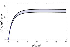
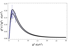
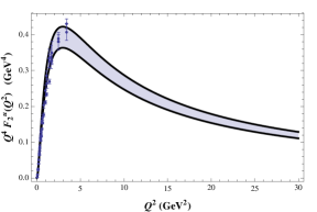
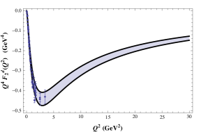
Figure 1: Dirac $u$ and $d$ quark form factors.

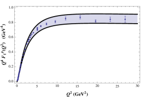
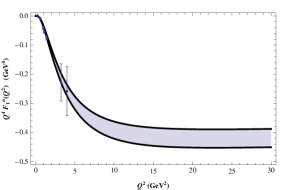
Figure 2: Pauli $u$ and $d$ quark form factors.

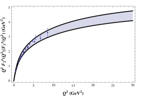
Figure 3: Proton and neutron Dirac form factors.

Figure 4: Ratio $Q^{2}F_{2}^{p}(Q^{2})/F_{1}^{p}(Q^{2})$ for proton.

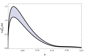
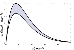
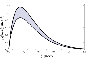
Figure 5: Gluon PDFs $xg_{1T}^{g}(x)$ and $xh_{1}^{\perp g}(x)$.

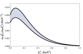
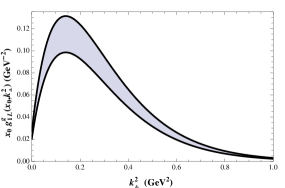
Figure 6: Gluon TMD $x_{0}f_{1}^{g}(x_{0},{\bf k}_{\perp}^{2})$ for $x_{0}=0.001$ (left panel) and for $x_{0}=0.1$ (right panel).

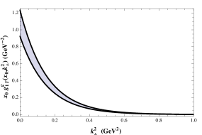
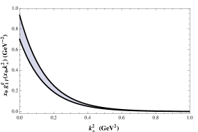
Figure 7: Gluon TMD $x_{0}g_{1L}^{g}(x_{0},{\bf k}_{\perp}^{2})$ for $x_{0}=0.001$ (left panel) and for $x_{0}=0.1$ (right panel).

Figure 8: Gluon TMD $x_{0}g_{1T}^{g}(x_{0},{\bf k}_{\perp}^{2})$ for $x_{0}=0.001$ (left panel) and for $x_{0}=0.1$ (right panel).

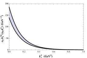
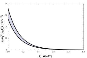
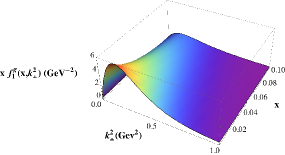
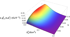
Figure 9: Gluon TMD $x_{0}h_{1}^{\perp g}(x_{0},{\bf k}_{\perp}^{2})$ for $x_{0}=0.001$ (left panel) and for $x_{0}=0.1$ (right panel).

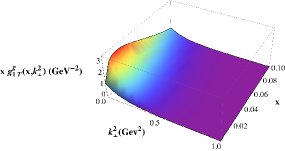
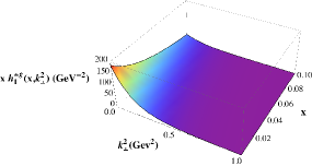
Figure 10: 3D plots of gluon TMDs $xf_{1}^{g}(x,{\bf k}_{\perp}^{2})$ (left panel) and $xg_{1L}^{g}(x,{\bf k}_{\perp}^{2})$ (right panel).

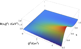
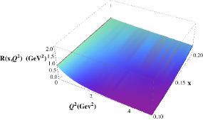
Figure 11: 3D plots of gluon TMDs $xg_{1T}^{g}(x,{\bf k}_{\perp}^{2})$ (left panel) and $xh_{1}^{\perp g}(x,{\bf k}_{\perp}^{2})$ (right panel).

Figure 12: 3D plots of the ratio $R(x,Q^{2})$ for gluon GPDs for $0.2\leq x\leq 1$ (left panel) and $0.1\leq x\leq 0.2$ (right panel).

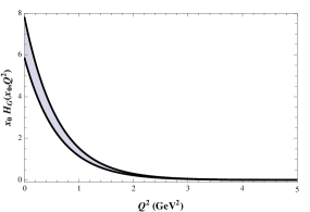
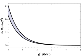
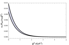
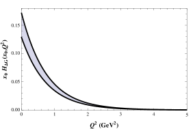
Figure 13: $Q^{2}$ dependence of the gluon GPD $x_{0}{\cal H}_{G}(x_{0},Q^{2})$ for $x_{0}=0.001$ (left panel) and for $x_{0}=0.1$ (right panel).

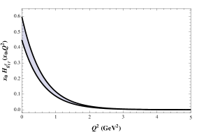
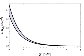
Figure 14: $Q^{2}$ dependence of the gluon GPD $x_{0}{\cal H}_{\Delta G}(x_{0},Q^{2})$ for $x_{0}=0.001$ (left panel) and for $x_{0}=0.1$ (right panel).

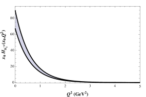
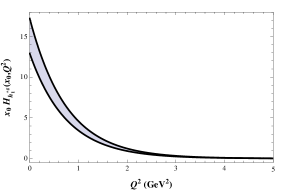
Figure 15: $Q^{2}$ dependence of the gluon GPD $x_{0}{\cal H}_{g_{1T}^{g}}(x_{0},Q^{2})$ for $x_{0}=0.001$ (left panel) and for $x_{0}=0.1$ (right panel).

Figure 16: $Q^{2}$ dependence of the gluon GPD $x_{0}{\cal H}_{f_{1}^{\perp g}}(x_{0},Q^{2})$ for $x_{0}=0.001$ (left panel) and for $x_{0}=0.1$ (right panel).

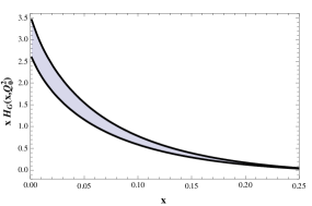
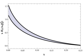
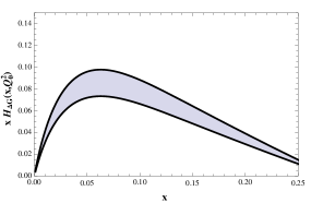
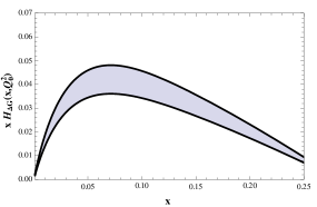
Figure 17: $x$ dependence of the gluon GPD $x{\cal H}_{G}(x,Q_{0}^{2})$ for $Q_{0}^{2}=0.5$ GeV² (left panel) and for $Q_{0}^{2}=1$ GeV² (right panel).

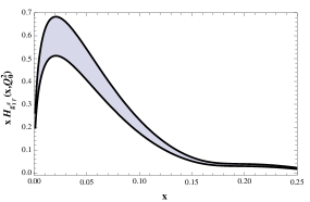
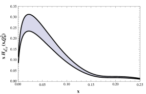
Figure 18: $x$ dependence of the gluon GPD $x{\cal H}_{\Delta G}(x,Q_{0}^{2})$ for $Q_{0}^{2}=0.5$ GeV² (left panel) and for $Q_{0}^{2}=1$ GeV² (right panel).

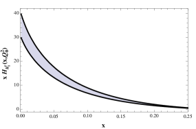
Figure 19: $x$ dependence of the gluon GPD $x{\cal H}_{g_{1T}^{g}}(x,Q_{0}^{2})$ for $Q_{0}^{2}=0.5$ GeV² (left panel) and for $Q_{0}^{2}=1$ GeV² (right panel).

Figure 20: $x$ dependence of the gluon GPD $x{\cal H}_{h_{1}^{\perp g}}(x,Q_{0}^{2})$ for $Q_{0}^{2}=0.5$ GeV² (left panel) and for $Q_{0}^{2}=1$ GeV² (right panel).

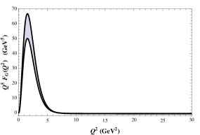
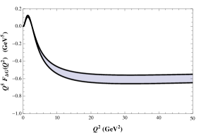
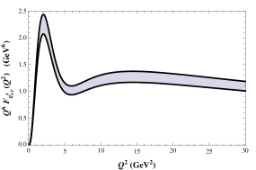
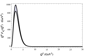
Figure 21: $Q^{2}$ dependence of the gluon form factors $Q^{5}F_{G}(Q^{2})$ (left panel) and $Q^{5}F_{\Delta G}(Q^{2})$ (right panel).

Figure 22: $Q^{2}$ dependence of the gluon form factors $Q^{6}F_{g_{1T}^{g}}(Q^{2})$ (left panel) and $Q^{6}F_{h_{1}^{\perp g}}(Q^{2})$ (right panel).

Next, it is interesting to compare the $Q^{2}$ dependence of our GPDs with the ones derived in Ref. Diehl:1998kh :

$${\cal H}_{G}(x,Q^{2}) = \ \ G(x)\ \exp\Big{[}-\frac{a_{g}^{2}}{2}\,\frac{1-x}{x}\,Q^{2}\Big{]}\,,$$

$${\cal H}_{\Delta G}(x,Q^{2}) = \Delta G(x)\ \exp\Big{[}-\frac{a_{g}^{2}}{2}\,\frac{1-x}{x}\,Q^{2}\Big{]}\,,$$ (165)

where $a_{g}=0.75$ GeV^-1 is the scale parameter. In both approaches the gluon GPDs are expressed in terms of gluon PDFs, therefore we just analyze the ratios of corresponding GPDs derived in Ref. Diehl:1998kh and by us:

$$R(x,Q^{2})=\frac{\exp\Big{[}-\frac{a_{g}^{2}}{2}\,\frac{1-x}{x}\,Q^{2}\Big{]}}{\exp\Big{[}-D_{g}(1-x)^{2}\frac{Q^{2}}{4\kappa^{2}}\Big{]}}\,,$$ (166)

where $D_{g}$ is the same parameter as used in the analysis of the gluon TMDs. One can see that exponential of the GPDs derived in our formalism has an extra fall off $(1-x)$, which is consistent with large scaling of the gluon form factors dictated by quark counting rules. In case of GPDs this extra fall off is not sufficient at large $x$, because the exponentials in both approaches becomes 1 at $x\to 1$ and the GPDs are determined by the corresponding PDF. In Figs. 12(a) and (b) we present a 3D plot of the ratio $R(x,Q^{2})$, as function of $x$ and $Q^{2}$. It is seen that two predictions for the gluon GPDs have very good agreement in the region $0.2\leq x\leq 1$, i.e. the ratio $R(x,Q^{2})\simeq 1$ and are differed at small $x\leq 0.2$. Note that the small $x$ behavior of the GPDs in our approach is consistent with small $x$ behavior of the PDFs and TMDs, which are in our approach are consistent with world data Ball:2017nwa ; Nocera:2014gqa and similar approaches Bacchetta:2020vty . On the other hand, as we stressed before, the similar approaches Meissner:2007rx ; Bacchetta:2008af ; Bacchetta:2020vty ; Kaur:2020pvc for quark and gluon TMDs and GPDs are consistent with us at small and intermediate $x$, while they have different large $x$ behavior inconsistent with counting rules. By the way, they can be easily improved by taking into account a specific $x$-dependence of the couplings/form factors. Such idea was proposed in Ref. Jakob:1997wg , where the spectator model was derived. In particular, it was suggested that the multipole form factors of spectator diquark contain a free parameter $\alpha$, which indicates the power of form factors and can be clearly fixed to fulfill large $x$ counting rules. Therefore, our approach has advantage that it is valid in whole region of $x$ and compatible respectively with approaches developed for specific regions of $x$.

In Figs. 16-20 we present our results for the GPDs. In particular, in Figs. 16-16 we display the $Q^{2}$ behavior of the gluon GPDs $x_{0}{\cal H}(x_{0},Q^{2})$ at fixed values of $x_{0}=0.001$ (left panel) and $x_{0}=0.1$ (right panel). In Figs. 20-20 we show the $x$ behavior of the gluon GPDs at fixed value of transversed momentum squared $Q_{0}^{2}=1$ GeV². As expected our curves for the gluon GPDs fall of with increasing $Q^{2}$ and vanish at $Q^{2}\simeq 2-3$ GeV². Finally, in Figs. 22 and 22 we show our predictions for the gluon form factors. In the plots we multiply each form factor with corresponding inverse power of $Q^{2}$ corresponding to the large $Q^{2}$ asymptotics. In particular, in Figs. 22(a), 22(b), 22(a), and 22(b) we present the results for $Q^{5}F_{G}(Q^{2})$, $Q^{5}F_{\Delta G}(Q^{2})$, $Q^{6}F_{g_{1T}^{g}}(Q^{2})$, and $Q^{6}F_{h_{1}^{\perp g}}(Q^{2})$, respectively. One can see that all form factors approach the corresponding large $Q^{2}$ asymptotics at $Q^{2}\sim 10$ GeV².

V Summary

In the present paper we have explicitly demonstrated how to correctly define gluon parton distributions (PDFs, TMDs, and GPDs) and form factors in the soft-wall AdS/QCD approach based on the use of quadratic dilaton. In the description of the partonic structure of hadrons our approach based on ideas of Refs. Brodsky:1989db ; Brodsky:1994kg ; Brodsky:2000ii ; Brodsky:2002cx ; Lyubovitskij:2020gjz and consistent with constraints imposed by QCD Drell:1969km ; Bloom:1970xb ; Brodsky:1973kr ; Blankenbecler:1974tm ; Yuan:2003fs ; Aicher:2010cb ; Mulders:2000sh . In particular, in the case of nucleons we derive the expressions for the T-even gluon TMDs in terms of LFWFs describing the gluon-three quark Fock component in the nucleon as bound state of struck gluon and three-quark core (spectator). Next using expressions of the PDFs in terms of LFWfs we can express all gluon parton densities in terms of the set of the gluon PDFs $G(x)$ and $\Delta G(x)$. We demonstrated that our formalism is consistent with model-independent derivation of the gluon correlators proposed in Ref. Mulders:2000sh and later considered in Ref. Meissner:2007rx ; Bacchetta:2020vty . We proved that our gluon TDMs obey the model-independent Mulders-Rodrigues inequalities Mulders:2000sh without referring to a choice of model parameters. As a new result we derived the sum rule involving four T-even TMDs (112), from which the Mulders-Rodrigues positivity bounds follow immediately. We checked that in similar approaches this sum rule is also fulfilled. E.g., in the spectator model considered in Ref. Bacchetta:2020vty the sum rule holds when the minimal coupling of gluon with three-quark spectator is used. In the quark target model discussed in Ref. Meissner:2007rx the sum rules is slightly different upon replacement of the nucleon mass by the constituent quark mass. For the first time, we derived results for the large $x$ behavior of the gluon TMDs, GPDs, and form factors. All gluon parton distributions are defined in terms of the unpolarized and polarized gluon PDFs. As numerical application we calculated the T-even gluon TMDs using as input the gluon PDFs extracted recently in Ref. Sufian:2020wcv based on ideas of QCD approaches Brodsky:1989db and Brodsky:1994kg and using world data analysis performed by the NNPDF Collaboration in Refs. Ball:2017nwa ; Nocera:2014gqa . We get very good of our results for the gluon TMDs with results of similar approach developed recently in Ref. Bacchetta:2020vty . To solidify our approach we calculated the electromagnetic form factors of nucleons induced by valence quark partonic densities and get perfect agreement with data Diehl:2013xca ; Cates:2011pz . Finally, we presented our predictions for the $x$ and $Q^{2}$ dependence of the gluon GPDs and $Q^{2}$ dependence of the gluon form factors.

In conclusion, we note that our approach for quark and gluon parton densities is very similar to the approaches developed in Refs. Jakob:1997wg ; Meissner:2007rx ; Bacchetta:2008af ; Bacchetta:2020vty ; Kaur:2020pvc . In case of quarks the consistency was shown in Ref. Bacchetta:2008af , while in case of gluons we discuss it in the present paper. E.g., it is supported by good agreement of description of the gluon TMDs in Ref. Bacchetta:2020vty and in our formalism. As advantage of our framework we mention that we are able to predict all parton densities using analytical formulas for the TMDs, GPDs, and form factors in terms of the set of PDFs, which are taken from world data analysis. Also we fulfill all constraints imposed by QCD including counting rules at large $x$. We should note that in similar approaches consistency with counting rules was not yet implemented. However, such possibility exists. In particular, in Ref. Jakob:1997wg , where the spectator model was proposed, it was suggested that the multipole form factors of spectator diquark contain a free parameter $\alpha$. This parameter indicates the power of form factors and can be clearly fixed to fulfill large $x$ counting rules.

Appendix A TMDs in the generalized version

Here we list the gluon TMDs in soft-wall AdS/QCD using generalized version for the LFWFs $\varphi^{(1)}$ and $\varphi^{(2)}$:

$$\varphi^{(1)}(x,{\bf k}_{\perp}^{2}) = \frac{4\pi}{\kappa}\,\sqrt{G^{+}(x)}\ \beta(x)\,\sqrt{D_{g_{1}}(x)}\,\exp\biggl{[}-\frac{{\bf k}_{\perp}^{2}}{2\kappa^{2}}\,D_{g_{1}}(x)\biggr{]}\,,$$ (167)

$$\frac{1}{M_{N}}\,\varphi^{(2)}(x,{\bf k}_{\perp}^{2}) = \frac{4\pi}{\kappa^{2}}\,\sqrt{G^{-}(x)}\,\frac{D_{g_{2}}(x)}{1-x}\,\exp\biggl{[}-\frac{{\bf k}_{\perp}^{2}}{2\kappa^{2}}\,D_{g_{2}}(x)\biggr{]}\,,$$ (168)

where $D_{g_{1}}(x)>0$ and $D_{g_{2}}(x)>0$ are the profile functions.

T-even gluon TMDs in the momentum ${\bf k}_{\perp}$ space:

$$f_{1}^{g}(x,{\bf k}_{\perp}^{2}) = \frac{1}{16\pi^{3}}\,\biggl{[}(\varphi^{(1)}(x,{\bf k}_{\perp})\Big{)}^{2}+\frac{{\bf k}_{\perp}^{2}}{M_{N}^{2}}\,\Big{(}1+(1-x)^{2}\Big{)}\,\Big{(}\varphi^{(2)}(x,{\bf k}_{\perp})\Big{)}^{2}\biggr{]}$$ (169)

$$= \biggl{[}G(x)+G^{-}(x)\,\alpha_{+}(x)\,\biggl{(}\frac{{\bf k}_{\perp}^{2}\,D_{g_{2}}^{2}(x)}{\kappa^{2}D_{g_{1}}(x)}-1\biggr{)}\,e^{-{\bf k}_{\perp}^{2}\Delta D_{g}(x)/\kappa^{2}}\biggr{]}\,\frac{D_{g_{1}}(x)}{\pi\kappa^{2}}\,\exp\biggl{[}-\frac{{\bf k}_{\perp}^{2}}{\kappa^{2}}D_{g_{1}}(x)\biggr{]}\,,$$

$$g_{1L}^{g}(x,{\bf k}_{\perp}) = \frac{1}{16\pi^{3}}\,\biggl{[}(\varphi^{(1)}(x,{\bf k}_{\perp})\Big{)}^{2}+\frac{{\bf k}_{\perp}^{2}}{M_{N}^{2}}\,\Big{(}1-(1-x)^{2}\Big{)}\,\Big{(}\varphi^{(2)}(x,{\bf k}_{\perp})\Big{)}^{2}\biggr{]}$$ (170)

$$= \biggl{[}\Delta G(x)+G^{-}(x)\,\alpha_{-}(x)\,\biggl{(}\frac{{\bf k}_{\perp}^{2}\,D_{g_{2}}^{2}(x)}{\kappa^{2}D_{g_{1}}(x)}-1\biggr{)}\,e^{-{\bf k}_{\perp}^{2}\Delta D_{g}(x)/\kappa^{2}}\biggr{]}\,\frac{D_{g_{1}}(x)}{\pi\kappa^{2}}\,\exp\biggl{[}-\frac{{\bf k}_{\perp}^{2}}{\kappa^{2}}D_{g_{1}}(x)\biggr{]}\,,$$

$$g_{1T}^{g}(x,{\bf k}_{\perp}^{2}) = \frac{1}{8\pi^{3}}\,\varphi^{(1)}(x,{\bf k}_{\perp})\,\varphi^{(2)}(x,{\bf k}_{\perp})\,(1-x)$$ (171)

$$= \sqrt{G^{2}(x)-\Delta G^{2}(x)}\,\beta(x)\,\frac{\sqrt{D_{g_{1}}(x)}\,D_{g_{2}}(x)M_{N}}{\pi\kappa^{3}}\,\,\exp\biggl{[}-\frac{{\bf k}_{\perp}^{2}}{2\kappa^{2}}\Big{(}D_{g_{1}}(x)+D_{g_{2}}(x)\Big{)}\biggr{]}$$

$$= g_{1T}^{g}(x)\ \frac{D_{g_{1}}(x)+D_{g_{2}}(x)}{2\pi\kappa^{2}}\,\exp\biggl{[}-\frac{{\bf k}_{\perp}^{2}}{2\kappa^{2}}\Big{(}D_{g_{1}}(x)+D_{g_{2}}(x)\Big{)}\biggr{]}\,,$$

$$h_{1}^{\perp g}(x,{\bf k}_{\perp}^{2}) = \frac{1}{4\pi^{3}}\,\Big{[}\varphi_{q}^{(2)}(x,{\bf k}_{\perp})\Big{]}^{2}\,(1-x)$$ (172)

$$= \frac{G(x)-\Delta G(x)}{1-x}\,\frac{2D^{2}_{g_{2}}(x)M_{N}^{2}}{\pi\kappa^{4}}\,\exp\biggl{[}-\frac{{\bf k}_{\perp}^{2}}{\kappa^{2}}\,D_{g_{2}}(x)\biggr{]}=h_{1}^{\perp g}(x)\ \frac{D_{g_{2}}(x)}{\pi\kappa^{2}}\,\exp\biggl{[}-\frac{{\bf k}_{\perp}^{2}}{\kappa^{2}}D_{g_{2}}(x)\biggr{]}\,,$$

where $\Delta D_{g}(x)=D_{g_{2}}(x)-D_{g_{1}}(x)$.

The gluon PDFs are written as:

$$f_{1}^{g}(x) = \int d^{2}{\bf k}_{\perp}\,f_{1}^{g}(x,{\bf k}_{\perp}^{2})=G(x)\,,$$

$$g_{1L}^{g}(x) = \int d^{2}{\bf k}_{\perp}\,g_{1L}^{g}(x,{\bf k}_{\perp}^{2})=\Delta G(x)\,,$$

$$g_{1T}^{g}(x) = \int d^{2}{\bf k}_{\perp}\,g_{1T}^{g}(x,{\bf k}_{\perp}^{2})=\frac{2\sqrt{D_{g_{1}}(x)}D_{g_{2}}(x)M_{N}}{\Big{[}D_{g_{1}}(x)+D_{g_{2}}(x)\Big{]}\kappa}\,\sqrt{G^{2}(x)-\Delta G^{2}(x)}\ \beta(x)\,,$$

$$h_{1}^{\perp g}(x) = \int d^{2}{\bf k}_{\perp}\,h_{1}^{\perp g}(x,{\bf k}_{\perp}^{2})=\frac{2D_{g_{2}}(x)M_{N}^{2}}{\kappa^{2}}\,\frac{G(x)-\Delta G(x)}{1-x}\,.$$ (173)

They obey the condition

$$\frac{\Big{[}g_{1T}^{g}(x)\Big{]}^{2}}{\Big{[}f_{1}^{g}(x)+g_{1L}^{g}(x)\Big{]}\,h_{1}^{\perp g}(x)}=\frac{2D_{g_{1}}(x)D_{g_{2}}(x)}{\Big{[}D_{g_{1}}(x)+D_{g_{2}}(x)\Big{]}^{2}}\,(1-x)\,\beta^{2}(x)\,.$$ (174)

The results for impact TMDs are expressed in terms of generalized impact LFWFs:

$$\tilde{\varphi}^{(1)}(x,{\bf b}_{\perp}^{2}) = \frac{1}{2\pi}\,\sqrt{G^{+}(x)}\ \beta(x)\,\exp\Big{[}-\frac{{\bf b}_{\perp}^{2}\kappa^{2}}{8D_{g_{1}}(x)}\Big{]}\,,$$ (175)

$$\tilde{\varphi}^{(2)}(x,{\bf b}_{\perp}^{2}) = \frac{1}{2\pi}\,\sqrt{G^{-}(x)}\,\frac{\sqrt{D_{g_{2}}(x)}}{1-x}\,\exp\Big{[}-\frac{{\bf b}_{\perp}^{2}\kappa^{2}}{8D_{g_{2}}(x)}\Big{]}\,.$$ (176)

In this case the expressions for the impact T-even gluon TMDs are given by:

$$\tilde{f}_{1}^{g}(x,{\bf b}_{\perp}^{2}) = \int\frac{d^{2}{\bf k}_{\perp}}{(2\pi)^{2}}\,e^{i{\bf b}_{\perp}{\bf k}_{\perp}}\,f_{1}^{g}(x,{\bf k}_{\perp}^{2})$$ (177)

$$= \Big{[}\tilde{\varphi}^{(1)}(x,{\bf b}_{\perp}^{2})\Big{]}^{2}+\Big{[}\tilde{\varphi}^{(2)}(x,{\bf b}_{\perp}^{2})\Big{]}^{2}\,\frac{1+(1-x)^{2}}{D_{g_{2}}(x)}\,\biggl{[}1+\frac{{\bf b}_{\perp}^{2}\kappa^{2}}{4D_{g_{2}}(x)}\biggr{]}$$

$$= \frac{1}{4\pi^{2}}\,\biggl{[}G(x)+G^{-}(x)\,\alpha_{+}(x)\,\gamma(x,{\bf b}_{\perp}^{2})\biggr{]}\,\exp\Big{[}-\frac{{\bf b}_{\perp}^{2}\kappa^{2}}{4D_{g_{1}}(x)}\Big{]}\,,$$

$$\tilde{g}_{1L}^{g}(x,{\bf b}_{\perp}^{2}) = \int\frac{d^{2}{\bf k}_{\perp}}{(2\pi)^{2}}\,e^{i{\bf b}_{\perp}{\bf k}_{\perp}}\,g_{1L}^{g}(x,{\bf k}_{\perp}^{2})$$ (178)

$$= \Big{[}\tilde{\varphi}^{(1)}(x,{\bf b}_{\perp}^{2})\Big{]}^{2}+\Big{[}\tilde{\varphi}^{(2)}(x,{\bf b}_{\perp}^{2})\Big{]}^{2}\,\frac{1-(1-x)^{2}}{D_{g_{2}}(x)}\,\biggl{[}1+\frac{{\bf b}_{\perp}^{2}\kappa^{2}}{4D_{g_{2}}(x)}\biggr{]}$$

$$= \frac{1}{4\pi^{2}}\,\biggl{[}\Delta G(x)+G^{-}(x)\,\alpha_{-}(x)\,\gamma(x,{\bf b}_{\perp}^{2})\biggr{]}\,\exp\Big{[}-\frac{{\bf b}_{\perp}^{2}\kappa^{2}}{4D_{g_{1}}(x)}\Big{]}\,,$$

$$\tilde{g}_{1T}^{g}(x,{\bf b}_{\perp}^{2}) = \int\frac{d^{2}{\bf k}_{\perp}}{(2\pi)^{2}}\,e^{i{\bf b}_{\perp}{\bf k}_{\perp}}\,g_{1T}^{g}(x,{\bf k}_{\perp}^{2})$$ (179)

$$= \frac{2M_{N}}{\kappa}\,\sigma(x,{\bf b}_{\perp}^{2})\,\tilde{\varphi}^{(1)}(x,{\bf b}_{\perp}^{2})\tilde{\varphi}^{(2)}(x,{\bf b}_{\perp}^{2})(1-x)$$

$$= \frac{1}{4\pi^{2}}\,g_{1T}^{g}(x)\,\exp\Big{[}-\frac{{\bf b}_{\perp}^{2}\kappa^{2}}{2(D_{g_{1}}(x)+D_{g_{2}}(x))}\Big{]}\,,$$

$$\tilde{h}_{1}^{\perp g}(x,{\bf b}_{\perp}^{2}) = \int\frac{d^{2}{\bf k}_{\perp}}{(2\pi)^{2}}\,e^{i{\bf b}_{\perp}{\bf k}_{\perp}}\,h_{1}^{\perp g}(x,{\bf k}_{\perp}^{2})$$ (180)

$$= \frac{4M_{N}^{2}}{\kappa^{2}}\,\Big{[}\tilde{\varphi}^{(2)}(x,{\bf b}_{\perp})\Big{]}^{2}\,(1-x)$$

$$= \frac{1}{4\pi^{2}}\,h_{1}^{\perp g}(x)\,\exp\Big{[}-\frac{{\bf b}_{\perp}^{2}\kappa^{2}}{4D_{g_{2}}(x)}\Big{]}\,,$$

where

$$\gamma(x,{\bf b}_{\perp}^{2}) = \biggl{[}1+\frac{{\bf b}_{\perp}^{2}\kappa^{2}}{4D_{g_{2}}(x)}\biggr{]}\,\exp\biggl{[}-\frac{{\bf b}_{\perp}^{2}\kappa}{4D_{g-}(x)}\biggr{]}\,,$$

$$\frac{1}{D_{g\pm}(x)} = \frac{1}{D_{g_{2}}(x)}\pm\frac{1}{D_{g_{1}}(x)}\,,$$

$$\sigma(x,{\bf b}_{\perp}^{2}) = \frac{2\sqrt{D_{g_{1}}(x)D_{g_{2}}(x)}}{D_{g_{1}}(x)+D_{g_{2}}(x)}\,\exp\biggl{[}-\frac{{\bf b}_{\perp}^{2}\kappa^{2}}{8}\,\frac{D_{g+}(x)}{D_{g-}^{2}(x)}\biggr{]}\,.$$ (181)

One should stress again that the Mulders-Rodrigues inequalities Mulders:2000sh in the momentum ${\bf k}_{\perp}$ space hold in our approach without referring to a choice of the LFWF functions and in both symmetric $D_{g_{1}}(x)=D_{g_{2}}=D_{g}(x)$ (III.2) and generalized $D_{g_{1}}(x)\neq D_{g_{2}}$ (167) case.

In impact ${\bf b}_{\perp}$ space one can also derive the inequalities between gluon TMDs, which involve profile functions $D_{g}$ functions and scale parameter $\kappa$. In symmetric case the inequalities were derived in Eqs. (139)-(141).

In the generalized case the gluon TMDs satisfy the following relations:

$$\tilde{g}_{1L}^{g}(x,{\bf b}_{\perp}^{2})\leq\tilde{f}_{1}^{g}(x,{\bf b}_{\perp}^{2})\,,$$ (182)

$$\tilde{g}_{1T}^{g}(x,{\bf b}_{\perp}^{2})\leq\frac{M_{N}}{\kappa}\,\sqrt{\frac{D_{g_{2}}(x)}{1+\frac{{\bf b}_{\perp}^{2}\kappa^{2}}{4D_{g_{2}}(x)}}}\,\tilde{f}_{1}^{g}(x,{\bf b}_{\perp}^{2})\leq\frac{M_{N}}{\kappa}\,\sqrt{D_{g_{2}}(x)}\,\tilde{f}_{1}^{g}(x,{\bf b}_{\perp}^{2})\,,$$ (183)

$$\tilde{h}_{1}^{\perp g}(x,{\bf b}_{\perp}^{2})\leq\frac{2M_{N}^{2}}{\kappa^{2}}\,\frac{D_{g_{2}}(x)}{1+\frac{{\bf b}_{\perp}^{2}\kappa^{2}}{4D_{g_{2}}(x)}}\,\tilde{f}_{1}^{g}(x,{\bf b}_{\perp}^{2})\leq\frac{2M_{N}^{2}}{\kappa^{2}}\,D_{g_{2}}(x)\,\tilde{f}_{1}^{g}(x,{\bf b}_{\perp}^{2})\,.$$ (184)

One can see that the first inequality (182) between $\tilde{g}_{1L}^{g}(x,{\bf b}_{\perp}^{2})$ and $\tilde{f}_{1}^{g}(x,{\bf b}_{\perp}^{2})$ is the same in both symmetric and generalized case and is similar to the one in momentum ${\bf k}_{\perp}$ space. The second (183) and third (184) inequalities involve the scale parameter $\kappa$ and profile function $D_{g_{2}}(x)$. In the limit $D_{g_{1}}(x)=D_{g_{2}}(x)=D_{g}(x)$ the inequalities (183) and (184) reduce to the inequalities (140) and (141) in the symmetric case.

The proof of the inequalities is straightforward. In particular, the inequality (182) follows from decomposition of $\tilde{f}_{1}^{g}(x,{\bf b}_{\perp}^{2})$ and $\tilde{g}_{1L}^{g}(x,{\bf b}_{\perp}^{2})$ in terms of the LFWFs $\tilde{\varphi}^{(i)}(x,{\bf b}_{\perp})$:

$$\tilde{f}_{1}^{g}(x,{\bf b}_{\perp}^{2})-\tilde{g}_{1L}^{g}(x,{\bf b}_{\perp}^{2})=2\Big{[}\tilde{\varphi}^{(2)}(x,{\bf b}_{\perp}^{2})\Big{]}^{2}\,\frac{(1-x)^{2}}{D_{g_{2}}(x)}\biggl{[}1+\frac{{\bf b}_{\perp}^{2}\kappa^{2}}{4D_{g_{2}}(x)}\biggr{]}\geq 0\,.$$ (185)

To derive the inequality (183) we start with inequality

$$\tilde{f}_{1}^{g}(x,{\bf b}_{\perp}^{2})-\frac{\kappa}{M_{N}\sigma(x,{\bf b}_{\perp}^{2})\sqrt{D_{g_{2}}(x)}}\,\sqrt{1+\frac{{\bf b}_{\perp}^{2}\kappa^{2}}{4D_{g_{2}}(x)}}\,\tilde{g}_{1T}^{g}(x,{\bf b}_{\perp}^{2})\geq 0\,,$$ (186)

which holds because it can be written in the form

$$\biggl{[}\tilde{\varphi}^{(1)}(x,{\bf b}_{\perp})-\tilde{\varphi}^{(2)}(x,{\bf b}_{\perp})\,\frac{1-x}{\sqrt{D_{g_{2}}(x)}}\,\sqrt{1+\frac{{\bf b}_{\perp}^{2}\kappa^{2}}{4D_{g_{2}}(x)}}\biggr{]}^{2}+\frac{1}{D_{g_{2}}(x)}\,\biggl{[}\tilde{\varphi}^{(2)}(x,{\bf b}_{\perp})\biggr{]}^{2}\,\biggl{[}1+\frac{{\bf b}_{\perp}^{2}\kappa^{2}}{4D_{g_{2}}(x)}\biggr{]}\geq 0\,.$$ (187)

Using inequalities (186),

$$\sigma(x,{\bf b}_{\perp}^{2})\leq\frac{2\sqrt{D_{g_{1}}(x)D_{g_{2}}(x)}}{D_{g_{1}}(x)+D_{g_{2}}(x)}\leq 1\,,\qquad\frac{1}{\sqrt{1+\frac{{\bf b}_{\perp}^{2}\kappa^{2}}{4D_{g_{2}}(x)}}}\leq 1$$ (188)

we arrive at Eq. (183).

To derive the inequality (184) we start with inequality

$$\tilde{f}_{1}^{g}(x,{\bf b}_{\perp}^{2})-\frac{\kappa^{2}}{2M_{N}^{2}D_{g_{2}}(x)}\,\biggl{[}1+\frac{{\bf b}_{\perp}^{2}\kappa^{2}}{4D_{g_{2}}(x)}\biggr{]}\,\tilde{h}_{1}^{\perp g}(x,{\bf b}_{\perp}^{2})\geq 0\,.$$ (189)

The latter inequality holds because it can be rewritten as

$$\biggl{[}\tilde{\varphi}^{(1)}(x,{\bf b}_{\perp})\biggr{]}^{2}+\biggl{[}\frac{x\,\tilde{\varphi}^{(2)}(x,{\bf b}_{\perp})}{\sqrt{D_{g_{2}}(x)}}\biggr{]}^{2}\,\biggl{[}1+\frac{{\bf b}_{\perp}^{2}\kappa^{2}}{4D_{g_{2}}(x)}\biggr{]}\geq 0\,.$$ (190)

Using inequalities (189) and

$$\frac{1}{1+\frac{{\bf b}_{\perp}^{2}\kappa^{2}}{4D_{g_{2}}(x)}}\leq 1$$ (191)

we arrive at Eq. (184).

References

• (1) A. Karch, E. Katz, D. T. Son, and M. A. Stephanov, Phys. Rev. D 74, 015005 (2006).
• (2) S. J. Brodsky and G. F. de Teramond, Phys. Rev. Lett.  96, 201601 (2006).
• (3) O. Andreev, Phys. Rev. D 73, 107901 (2006).
• (4) S. J. Brodsky, G. F. de Teramond, H. G. Dosch, and J. Erlich, Phys. Rep.  584, 1 (2015).
• (5) S. J. Brodsky and G. R. Farrar, Phys. Rev. Lett.  31, 1153 (1973); V. A. Matveev, R. M. Muradyan, and A. N. Tavkhelidze, Lett. Nuovo Cimento   5, 907 (1972) [Teor. Mat. Fiz.  15, 332 (1973)].
• (6) S. J. Brodsky and G. F. de Teramond, Phys. Rev. D 77, 056007 (2008).
• (7) Z. Abidin and C. E. Carlson, Phys. Rev. D 79, 115003 (2009).
• (8) A. Vega, I. Schmidt, T. Gutsche, and V. E. Lyubovitskij, Phys. Rev. D 83, 036001 (2011).
• (9) T. Branz, T. Gutsche, V. E. Lyubovitskij, I. Schmidt, and A. Vega, Phys. Rev. D 82, 074022 (2010).
• (10) S. J. Brodsky, F. G. Cao, and G. F. de Teramond, Phys. Rev. D 84, 075012 (2011).
• (11) T. Gutsche, V. E. Lyubovitskij, I. Schmidt, and A. Vega, Phys. Rev. D 85, 076003 (2012).
• (12) T. Gutsche, V. E. Lyubovitskij, and I. Schmidt, Nucl. Phys. B952, 114934 (2020); T. Gutsche, V. E. Lyubovitskij, I. Schmidt, and A. Vega, Phys. Rev. D 87, 016017 (2013).
• (13) T. Gutsche, V. E. Lyubovitskij, I. Schmidt, and A. Vega, Phys. Rev. D 86, 036007 (2012); 91, 114001 (2015).
• (14) T. Gutsche, V. E. Lyubovitskij, and I. Schmidt, Phys. Rev. D 94, 116006 (2016); 97, 054011 (2018); 101, 034026 (2020).
• (15) V. E. Lyubovitskij and I. Schmidt, Phys. Rev. D 102, 094008 (2020).
• (16) H. W. Lin et al., Prog. Part. Nucl. Phys.  100, 107 (2018).
• (17) M. Constantinou et al., arXiv:2006.08636 [hep-ph].
• (18) R. Angeles-Martinez et al., Acta Phys. Pol. B 46, 2501 (2015).
• (19) M. Diehl and P. Kroll, Eur. Phys. J. C 73, 2397 (2013).
• (20) D. Boer et al., arXiv:1108.1713 [nucl-th].
• (21) S. D. Drell and T. M. Yan, Phys. Rev. Lett.  24, 181 (1970).
• (22) E. D. Bloom and F. J. Gilman, Phys. Rev. Lett.  25, 1140 (1970).
• (23) R. Blankenbecler and S. J. Brodsky, Phys. Rev. D 10, 2973 (1974).
• (24) F. Yuan, Phys. Rev. D 69, 051501(R) (2004).
• (25) M. Aicher, A. Schafer, and W. Vogelsang, Phys. Rev. Lett.  105, 252003 (2010).
• (26) J. S. Conway, C. E. Adolphsen, J. P. Alexander, K. J. Anderson, J. G. Heinrich, J. E. Pilcher, A. Possoz, E. I. Rosenberg et al., Phys. Rev. D 39, 92 (1989).
• (27) S. J. Brodsky and I. A. Schmidt, Phys. Lett. B 234, 144 (1990).
• (28) S. J. Brodsky, M. Burkardt, and I. Schmidt, Nucl. Phys. B441, 197 (1995).
• (29) J. D. Bjorken, Phys. Rev. D 1, 1376 (1970).
• (30) V. N. Gribov and L. N. Lipatov, Yad. Fiz.  15, 781 (1972) [Sov. J. Nucl. Phys.  15, 438 (1972)]; Yad. Fiz.  15, 1218 (1972) [Sov. J. Nucl. Phys.  15, 675 (1972)].
• (31) S. J. Brodsky, J. R. Ellis, and M. Karliner, Phys. Lett. B 206, 309 (1988).
• (32) J. P. Ralston and D. E. Soper, Nucl. Phys. B152, 109 (1979); J. C. Collins and D. E. Soper, Nucl. Phys. B193, 381 (1981); B213, 545(E) (1983); D. W. Sivers, Phys. Rev. D 41, 83 (1990); R. D. Tangerman and P. J. Mulders, Phys. Rev. D 51, 3357 (1995); D. Boer and P. J. Mulders, Phys. Rev. D 57, 5780 (1998); J. C. Collins, Phys. Lett. B 536, 43 (2002).
• (33) S. J. Brodsky, D. S. Hwang, and I. Schmidt, Phys. Lett. B 530, 99 (2002).
• (34) P. J. Mulders and J. Rodrigues, Phys. Rev. D 63, 094021 (2001).
• (35) S. Meissner, A. Metz, and K. Goeke, Phys. Rev. D 76, 034002 (2007).
• (36) D. Boer, W. J. den Dunnen, C. Pisano, M. Schlegel, and W. Vogelsang, Phys. Rev. Lett.  108, 032002 (2012).
• (37) C. Lorcé and B. Pasquini, J. High Energy Phys. 09 (2013) 138.
• (38) Z. Lu and B. Q. Ma, Phys. Rev. D 94, 094022 (2016).
• (39) D. Boer, S. Cotogno, T. van Daal, P. J. Mulders, A. Signori, and Y. J. Zhou, J. High Energy Phys. 10 (2016) 013.
• (40) A. Bacchetta, F. G. Celiberto, M. Radici, and P. Taels, Eur. Phys. J. C 80, 733 (2020).
• (41) A. Bacchetta, D. Boer, C. Pisano, and P. Taels, Eur. Phys. J. C 80, 72 (2020).
• (42) C. Alexandrou, S. Bacchio, M. Constantinou, J. Finkenrath, K. Hadjiyiannakou, K. Jansen, G. Koutsou, H. Panagopoulos, and G. Spanoudes, Phys. Rev. D 101, 094513 (2020).
• (43) N. Kaur and H. Dahiya, DAE Symp. Nucl. Phys.  64, 641 (2020).
• (44) A. Vega, I. Schmidt, T. Branz, T. Gutsche, and V. E. Lyubovitskij, Phys. Rev. D 80, 055014 (2009).
• (45) V. E. Lyubovitskij, Invited talk at the Int. Conf. “Venturing off the lightcone - local versus global features (Light Cone 2013)” 20-24 May 2013, Skiathos, Greece; V. E. Lyubovitskij, T. Gutsche, I. Schmidt, and A. Vega, Few Body Syst.  55, 447 (2014).
• (46) G. F. de Teramond, T. Liu, R. S. Sufian, H. G. Dosch, S. J. Brodsky, and A. Deur (HLFHS Collaboration), Phys. Rev. Lett.  120, 182001 (2018).
• (47) S. J. Brodsky, G. F. de Teramond, and H. G. Dosch, arXiv:2004.07756 [hep-ph].
• (48) V. E. Lyubovitskij and I. Schmidt, Phys. Rev. D 102, 034011 (2020).
• (49) T. Gutsche, V. E. Lyubovitskij, I. Schmidt, and A. Vega, Phys. Rev. D 89, 054033 (2014), 92, 019902(E) (2015); A. Vega, I. Schmidt, T. Gutsche, and V. E. Lyubovitskij, arXiv:1306.1597 [hep-ph].
• (50) T. Gutsche, V. E. Lyubovitskij, I. Schmidt, and A. Vega, J. Phys. G 42, 095005 (2015).
• (51) T. Gutsche, V. E. Lyubovitskij, I. Schmidt, and A. Vega, Phys. Rev. D 91, 054028 (2015).
• (52) T. Gutsche, V. E. Lyubovitskij, and I. Schmidt, Eur. Phys. J. C 77, 86 (2017).
• (53) A. Vega and M. Angel Martin Contreras, Phys. Rev. D 102, 036017 (2020).
• (54) L. Chang, K. Raya, and X. Wang, Chin. Phys. C 44, 114105 (2020).
• (55) H. R. Grigoryan and A. V. Radyushkin, Phys. Rev. D 76, 095007 (2007).
• (56) A. D. Martin, W. J. Stirling, R. S. Thornem, and G. Watt, Eur. Phys. J. C 63, 189 (2009).
• (57) M. Gluck, E. Reya, and A. Vogt, Z. Phys. C 53, 651 (1992).
• (58) I. Novikov et al. (xFitter Developers Team), Phys. Rev. D 102, 014040 (2020).
• (59) S. J. Brodsky, D. S. Hwang, B. Q. Ma, and I. Schmidt, Nucl. Phys. B593, 311 (2001).
• (60) A. Bacchetta, F. Conti, and M. Radici, Phys. Rev. D 78, 074010 (2008).
• (61) M. Diehl and P. Hagler, Eur. Phys. J. C 44, 87 (2005).
• (62) M. Anselmino, D. Boer, U. D’Alesio, and F. Murgia, Phys. Rev. D 65, 114014 (2002).
• (63) P. Schweitzer, T. Teckentrup, and A. Metz, Phys. Rev. D 81, 094019 (2010).
• (64) M. Diehl, T. Feldmann, R. Jakob, and P. Kroll, Eur. Phys. J. C 8, 409 (1999); M. Diehl, Phys. Rep.  388, 41 (2003)
• (65) R. S. Sufian, T. Liu and A. Paul, Phys. Rev. D 103, 036007 (2021)
• (66) R. D. Ball et al. (NNPDF Collaboration), Eur. Phys. J. C 77, 663 (2017)
• (67) E. R. Nocera et al. (NNPDF Collaboration), Nucl. Phys. B887, 276 (2014).
• (68) M. Glück, E. Reya, and A. Vogt, Eur. Phys. J. C 5, 461 (1998).
• (69) M. Glück, E. Reya, M. Stratmann, and W. Vogelsang, Phys. Rev. D 63, 094005 (2001).
• (70) G. D. Cates, C. W. de Jager, S. Riordan, and B. Wojtsekhowski, Phys. Rev. Lett.  106, 252003 (2011).
• (71) R. Jakob, P. J. Mulders, and J. Rodrigues, Nucl. Phys. A626, 937 (1997).