Algebraic Approximations of a Polyhedron Correlation Function Stemming from its Chord Length Distribution

Abstract

An algebraic approximation, of order $K$, of a polyhedron correlation function (CF) can be obtained from $\gamma^{{}^{\prime\prime}}(r)$, its chord-length distribution (CLD), considering first, within the subinterval $[D_{i-1},\,D_{i}]$ of the full range of distances, a polynomial in the two variables $(r-D_{i-1})^{1/2}$ and $(D_{i}-r)^{1/2}$ such that its expansions around $r=D_{i-1}$ and $r=D_{i}$ simultaneously coincide with left and the right expansions of $\gamma^{{}^{\prime\prime}}(r)$ around $D_{i-1}$ and $D_{i}$ up to the terms $O\big{(}r-D_{i-1}\big{)}^{K/2}$ and $O\big{(}D_{i}-r\big{)}^{K/2}$, respectively. Then, for each $i$, one integrates twice the polynomial and determines the integration constants matching the resulting integrals at the common end points. The 3D Fourier transform of the resulting algebraic CF approximation correctly reproduces, at large $q$s, the asymptotic behaviour of the exact form factor up to the term $O(q^{-(K/2+4)})$. For illustration, the procedure is applied to the cube, the tetrahedron and the octahedron.

Synopsis We report a procedure for obtaining an algebraic approximation of the correlation function of a polyhedron starting from its known chord length distribution.

Keywords: small-angle scattering, polyhedra, chord-length distribution, correlation function, asymptotic behavior

To be published in Acta Cryst. A77,..,(2021),

https://doi.org/10.1107/S2053273320014229

1 - Introduction
Nowadays, the correlations functions (CF) [$\gamma(r)$] of the first three Platonic solids are explicitely known. In fact, Goodisman (1980) directly obtained the cube CF by evaluating the angular average of the overlapping volume while Ciccariello, starting from the general integral expression of the CF’s 2nd order derivative (Ciccariello et al., 1981), first worked out the explicit expressions of the CLDs of the tetrahedron (2005a) and the octahedron (2014a), and later succeeded in integrating these CLDs to get the corresponding CFs (2014b). The expressions of these CFs are not simple and take different forms within each of the $M$ subintervals of the full range of distances $[0,\,D_{M}]$. {For $i=1,\ldots,M$. the $i$th subinterval is defined as $[D_{i-1},\,D_{i}]$ (with $D_{0}\equiv 0$), its length is denoted by $\Delta_{i}\equiv(D_{i}-D_{i-1})$ while the $D_{i}$s are some of the distance values between vertices, between vertices and sides, and between the sides of the given polyhedron.} However, within each subinterval, the CFs are analytic functions of $r$ and their structure always is a sum of rational functions and of inverse trigonometric functions, the arguments of which also are rational functions. The last functions have the form $R(r,y)\equiv P(r,y)/Q(r,y)$ where $P$ and $Q$ are polynomials and $y$ denotesthe square root of a 2nd degree polynomial of $r$. Hence the important property: the derivatives of this kind of functions, whatever their order, are functions of the same kind. Quite recently, Ciccariello (2020a,b) has shown that the mentioned mathematical structure also applies to the CLD of any bounded polyhedron, whatever its shape. However, the related CFs are, as yet, not eplicitly known owing to the difficulty of twice integrating the CLDs in a closed analytic form.
In his report on the ms. of Ciccariello (2020b) paper one of the referees raised an important question, namely: whether it is possible to get an approximate algebraic expression of the CF stemming from the reported CLD. In this short note we present a procedure that achieves this aim through the following steps. Consider for definitenss the $i$th subinterval. Since we know the analytic form of the CLD inside each subinterval, we also know its right and left expansions respectively around the two end points $D_{i-1}$ and $D_{i}$ of the considered interval. The truncation of the two expansions yield two algebraic expressions which respectively approximate the CLD around $D_{i-1}$ and $D_{i}$. The difficulty now is that of devising a single algebraic function which simultaneously almost coincides with the truncated right expansion as $r\to D_{i-1}$ and with the left truncated expansion as $r\to D_{i}$. This problem is solved in the following section. The resulting function yields an algebraic approximation of the CLD within the full $i$th interval and its accuracy generally depends on the truncation order $K$. Integrating twice the resulting function we obtain an algebraic approximation of the CF within the same subinterval once we have determined the two integration constants. This determination is achieved by matching the CF approximations relevant to, say, the $i$th and the $(i+1)$th subintervals at the common end-point $D_{i}$. (The details of the procedure are reported in the second part of section 2.) Then, the sought for algebraic approximation of the full CF results from the combination of all these subinterval approximations. Section 3 applies the procedure to the known CFs mentioned at the beginning. In this way it is also possible to investigate how the accuracy depends on $K$. In this connection, we recall a theorem by Erdeĺiy (1956) according to which, at large $q$s, the leading asymptotic term of $\int_{.}^{D}(D-x)^{a}e^{iqx}dx$, with $a>-1$, is $\propto e^{iqD}/q^{a+1}$ (confining ourselves to the only contribution related to the reported integration limit). It follows that the truncation order increase makes the behaviour of the 3D Fourier transform of the CF approximation more accurate in the region of large scattering vectors.

2 - Procedure for generating an approximated CF from the CLD
The mentioned mathematical structure of any polyhedron’s CLD implies that this is analytic within each $r$-subinterval and that, within any right or left (small) neighbourhouds of $D_{i}$, its expansion reads

$$\gamma"(r)={{\mathfrak{D}}^{\pm}}_{i}(r)=\sum_{j=0}^{\infty}\Big{(}{a^{\pm}}_{i,j}\,|r-D_{i}|^{j}+{b^{\pm}}_{i,j}|r-{D_{i}}|^{j+1/2}\Big{)},$$ (1)

where superscript ⁺ applies if $r\to{D_{i}}^{+}$ (and superscript ^- if $r\to{D_{i}}^{-}$). The above series, truncated at $j=K$, will be denoted as ${\mathfrak{D}}^{\pm}_{i,K}(r)$, i.e.

$${\mathfrak{D}}^{\pm}_{i,K}(r)\equiv\sum_{j=0}^{K}\Big{(}{a^{\pm}}_{i,j}\,|r-D_{i}|^{j}+{b^{\pm}}_{i,j}|r-{D_{i}}|^{j+1/2}\Big{)}.$$ (2)

[Clearly, approximating ${{\mathfrak{D}}^{+}}_{i}(r)$ by ${\mathfrak{D}}^{+}_{i,K}(r)$ involves an error which is $O(|r-D_{i}|^{K+1})$ within a small right-neighbourhoud of $D_{i}$. The same happens for ${{\mathfrak{D}}^{-}}_{i}(r)$.] We introduce now the new positive variables $\xi_{i}$ and $\eta_{i}$ according to the definitions

$$\xi_{i}(r)\equiv{(r-D_{i-1})^{1/2}},\quad\eta_{i}(r)\equiv({D_{i}-r})^{1/2}.$$ (3)

They are not independent since they are related by

$$\xi_{i}^{2}+\eta_{i}^{2}=\Delta_{i},$$ (4)

so that $\eta_{i}\to\Delta_{i}^{1/2}$ if $\xi_{i}\to 0$ or $r\to D_{i-1}^{+}$ and $\xi_{i}\to\Delta_{i}^{1/2}$ if $\eta_{i}\to 0$ or $r\to{D_{i}}^{-}$. In terms of $\xi_{i}$ and $\eta_{i}$, from (2) follows that ${\mathfrak{D}}^{+}_{i-1,K}(r)$ and ${\mathfrak{D}}^{-}_{i,K}(r)$ respectively take the forms

$${\mathfrak{D}}^{+}_{i-1,K}(r) = \sum_{j=0}^{K}\Big{(}{a^{+}}_{i-1,j}\,\xi_{i}^{2j}+{b^{+}}_{i-1,j}\xi_{i}^{2j+1}\Big{)},$$ (5)

$${\mathfrak{D}}^{-}_{i,K}(r) = \sum_{j=0}^{K}\Big{(}{a^{-}}_{i,j}\,\eta_{i}^{2j}+{b^{-}}_{i,j}\eta_{i}^{2j+1}\Big{)}$$ (6)

so that they respectively are polynomials of degree $(2K+1)$ of $\xi_{i}$ and $\eta_{i}$. Now, if we find a polynomial ${{\mathfrak{G}}}^{[2]}_{i,K}(r)$ of $(\xi_{i},\,\eta_{i})$ such that it behaves as ${{\mathfrak{D}}^{+}}_{i-1}(r)$ [up to the term $O(\xi_{i})^{2K}$ included], as $r\to D_{i-1}^{+}$, and as ${{\mathfrak{D}}^{-}}_{i}(r)$ [up to the term $O(\eta_{i})^{2K}$ included] as $r\to D_{i}^{-}$, according to what stated in section 1, ${{\mathfrak{G}}}^{[2]}_{i,K}(r)$ yields an algebraic approximation of $\gamma"(r)$ throughout the $i$th subinterval with an error $\propto\Delta_{i}^{K}$. To determine ${{\mathfrak{G}}}^{[2]}_{i,K}(r)$ we put

$${{\mathfrak{G}}}^{[2]}_{i,K}(r)\ \equiv \ {{\mathfrak{G}}}^{[2]}_{L,i,K}(r)+{{\mathfrak{G}}}^{[2]}_{R,i,K},$$ (7)

with

$${{\mathfrak{G}}}^{[2]}_{L,i,K}(r) \equiv \big{[}1+\xi^{2K+1}\,P_{L,i,K}(\eta)\big{]}{\mathfrak{D}}^{+}_{i-1,K}(r),$$ (8)

$${{\mathfrak{G}}}^{[2]}_{R,i,K}(r) \equiv \big{[}1+\eta^{2K+1}\,P_{R,i,K}(\xi)\big{]}\,{\mathfrak{D}}^{-}_{i,K}(r)$$ (9)

where, for notational simplicity, we omit to append index $i$ to $\xi$ and $\eta$. $P_{L,i,K}(\cdot)$ and $P_{R,i,K}(\cdot)$ are two unknown polynomials to be determined. Contribution ${{\mathfrak{G}}}^{[2]}_{L,i,K}(r)$ behaves as ${\mathfrak{D}}^{+}_{i-1,K}(r)$ as $r\to{D_{i-1}}^{+}$ up to the term $O(\xi^{2K})$ included. Similarly, as $r\to{D_{i}}^{-}$, ${{\mathfrak{G}}}^{[2]}_{R,i,K}(r)$ behaves as ${\mathfrak{D}}^{-}_{i,K}(r)$ up to the term $O(\eta^{2K})$. Hence, ${{\mathfrak{G}}}^{[2]}_{i,K}(r)$ is the sought for approximation if ${{\mathfrak{G}}}^{[2]}_{L,i,K}(r)$ is $o(\eta^{2K})$ as $r\to{D_{i}}^{-}$ and ${{\mathfrak{G}}}^{[2]}_{R,i,K}(r)$ is $o(\xi^{2K})$ as $r\to{D_{i-1}}^{+}$. The last two conditions uniquely determine the unknown polynomials. In fact, by (4) and (2), ${{\mathfrak{G}}}^{[2]}_{L,i,K}(r)$ around ${D_{i}}^{-}$ takes the form

$${{\mathfrak{G}}}^{[2]}_{L,i,K}(r)=\big{[}1+(\Delta-\eta^{2})^{K}(\Delta-\eta^{2})^{1/2}\,P_{L,i,K}(\eta)\big{]}\times$$ (10)

$$\sum_{j=0}^{K}\Big{[}{a^{+}}_{i-1,2j}\,(\Delta-\eta^{2})^{j}+{b^{+}}_{i-1,2j+1}(\Delta-\eta^{2})^{j}\,(\Delta-\eta^{2})^{1/2}\Big{]}.$$

We must require that its expansion around $\eta=0$ does not involve terms $O(\eta^{l})$ with $l\leq 2K$. This property must necessarily hold true for the expansion of the first factor present on the right hand side of (10). Since the expansions of $(\Delta-\eta^{2})^{K}$ and $(\Delta-\eta^{2})^{1/2}$ only involve even powers of $\eta$, the polynomial $P_{L,i,K}(\eta)$ must have the form: $\sum_{h=0}^{K}p_{h}\eta^{2h}$. The unknown coefficients $p_{0},\,p_{1},\ldots,p_{K}$ are iteratively determined solving the set of equations

$$\delta_{h,0}+\sum_{l=0}^{h}\frac{(-)^{h-l}p_{2l}}{\Delta^{h-l-K-1/2}}\sum_{q=0}^{{\rm{min}}[K,h-l]}\binom{K}{q}\binom{1/2}{h-q-l}=0,\ \ h=0,1,\ldots,K,$$ (11)

resulting from the expansion of the mentioned factor. (In the above relation, $\delta_{h,0}$ is the Kronecker symbol.) The remaining polynomial $P_{R,i,K}(\cdot)$ is determined by a similar procedure considering the expansion of ${{\mathfrak{G}}}^{[2]}_{R,i,K}(r)$ around $\xi=0$. In this way, the algebraic function ${{\mathfrak{G}}}^{[2]}_{i,K}(r)$, approximating the CLD within the $i$th subinterval, is fully determined.
To get, within the $i$th subinterval, the corresponding algebraic approximation of the CF, denoted by ${{\mathfrak{G}}}_{i,K}(r)$, it is sufficient to integrate twice the obtained ${{\mathfrak{G}}}^{[2]}_{i,K}(r)$, i.e.

$${{\mathfrak{G}}}_{i,K}(r) \equiv \int_{D_{i-1}}^{r}dx\int_{D_{i-1}}^{x}{{\mathfrak{G}}}^{[2]}_{i,K}(y)dy+A_{i}+B_{i}\ r=$$ (12)

$$\quad\int_{r}^{D_{i}}dx\int_{x}^{D_{i}}{{\mathfrak{G}}}^{[2]}_{i,K}(y)dy+A^{\prime}_{i}+B^{\prime}_{i}\ r,$$ (13)

where $A_{i},\,B_{i},\,A^{\prime}_{i}$ and $B^{\prime}_{i}$ are arbitrary constants. We underline that the previous integrals are algebraic functions because their expanded integrands only involve a single radical, associated either to the odd powers of $\xi$ or to the odd powers of $\eta$. The determination of ${{\mathfrak{G}}}_{i,K}(r)$ requires the determination of constants $A_{i}$ and $B_{i}$ or $A^{\prime}_{i}$ and $B^{\prime}_{i}$. This is made possible by the properties that the CF and its first derivative $\gamma^{{}^{\prime}}(r)$ are continuous within the full $r$-range $[0,\,D_{M}]$. [These properties follow from the general integral expressions of $\gamma(r)$ and $\gamma^{{}^{\prime}}(r)$, respectively reported by Guinier & Fournet(1955) and Ciccariello et al.  (1981).] We ecall now a general result (Ciccariello & Sobry, 1995) according to which the CLD of any polyhedron is a first degree $r$-polynomial in the innermost range of distances, i.e. $[0,\,D_{1}]$, and is, therefore, fully known because the relevant constant and the slope respectively are the polyhedron’s angularity and sharpness. Further, the angularity is related to the edges’ lengths and the corresponding dihedral angles by equation (4.5) of Ciccariello et al.  (1981) , while the sharpness is the sum of the contributions arising from each vertex of the considered polyhedron. The general expression of each of the last contributions depends on the angles between the edges converging into a vertex as well as on the relevant dihedral angles, and is given by equation (3.13) of Ciccariello and Sobry (1995). Adding to these results two further properties, namely i) $\gamma(0)=1$ and ii) $\gamma^{\prime}(0)=-S/4V$ (related to the Porod law because $S$ and $V$ respectively denote the surface area and the volume of the polyhedron), we conclude that the CF of a polyhedron always is fully known inside $[0,\,D_{1}]$. Constants $A_{i}$ and $B_{i}$ are determined proceeding as follows. From (12) and the last two mentioned properties follows that

$${{\mathfrak{G}}}_{1}(r)=1-S\,r/4V+{\cal A}r^{2}/2+{{\cal S}}r^{3}/3\approx\int_{0}^{r}dx\int_{0}^{x}{{\mathfrak{G}}}^{[2]}_{1,K}(y)dy$$ (14)

where ${\cal A}$ and ${\cal S}$ respectively denote the angularity and the sharpness. [We have omitted index $K$ because the first equality is exact.] In the same way, the continuity properties of $\gamma(r)$ and $\gamma^{\prime}(r)$ at $r=D_{M}$ imply that these two functions vanish at $D_{M}$. Thus, from (13) it follows that

$${{\mathfrak{G}}}_{M,K}(r)=\int_{r}^{D_{M}}dx\int_{x}^{D_{M}}{{\mathfrak{G}}}^{[2]}_{M,K}(y)dy.$$ (15)

Having fully determined both ${{\mathfrak{G}}}_{1,K}(r)$ and ${{\mathfrak{G}}}_{M,K}(r)$ we proceed to determining the remaining constants. Constants $A_{2}$ and $B_{2}$, present in the ${{\mathfrak{G}}}_{2,K}(r)$ definition, are uniquely determined by continuously matching ${{\mathfrak{G}}}_{2,K}(r)$ to ${{\mathfrak{G}}}_{1}(r)$ at $r=D_{1}$, i.e.  by requiring that

$$\lim_{r\to{D_{1}}^{+}}{{\mathfrak{G}}}_{2,K}(r) = \lim_{r\to{D_{1}}^{-}}{{\mathfrak{G}}}_{1}(r),$$ (16)

$$\lim_{r\to{D_{1}}^{+}}\frac{d{{\mathfrak{G}}}_{2,K}(r)}{dr} = \lim_{r\to{D_{1}}^{-}}\frac{d{{\mathfrak{G}}}_{1}(r)}{dr},$$ (17)

so that, by (12),

$$B_{2}=\lim_{r\to{D_{1}}^{-}}\frac{d{{\mathfrak{G}}}_{1}(r)}{dr}\quad{\rm and}\quad A_{2}=\lim_{r\to{D_{1}}^{-}}{{\mathfrak{G}}}_{1}(r)-B_{2}\,D_{1}.$$ (18)

and ${{\mathfrak{G}}}_{2,K}(r)$ also is fully determined. Iterating the procedure, we successively determine ${{\mathfrak{G}}}_{3,K}(r)$, ${{\mathfrak{G}}}_{4,K}(r),\ldots$ and, finally, ${{\mathfrak{G}}}_{M,K}(r)$, making apparently useless its previous determination reported in (15). However, each step of the recursive determination introduces an error and the errors sum up as the iteration goes on. Hence, it is reasonable to expect that the ${{\mathfrak{G}}}_{M,K}(r)$, obtained in the last step of the recursive chain, does not vanish, together with its derivative, at $r=D_{M}$ as it is required by (15). Thus, to reduce the approximation errors, it is more convenient to start from ${{\mathfrak{G}}}_{1,K}(r)$ and, proceeding towards the right, to successively determine ${{\mathfrak{G}}}_{2,K}(r),\dots,{{\mathfrak{G}}}_{i,K}(r)$ and then, starting from the ${{\mathfrak{G}}}_{M,K}(r)$, given by (15), and, proceeding towards the left, to successively determine ${{\mathfrak{G}}}_{M-1,K}(r),\ldots,{{\mathfrak{G}}}_{i+1,K}(r)$. For the reason already noted, it is extremely unlike that ${{\mathfrak{G}}}_{i,K}(r)$ exactly matches ${{\mathfrak{G}}}_{i+1,K}(r)$ at the point $r=D_{i}$. Nonetheless, their matching is still possible by suitably modifying the definition of one of them. To this aim, we observe that adding to ${{\mathfrak{G}}}^{[2]}_{i+1,K}(r)$ an extra contribution of the form

$${\mathfrak{C}}_{i+1,K}^{[2]}(r)\equiv(r-D_{i})^{K+1}(D_{i+1}-r)^{K+1}(\alpha+\beta\,r)=\xi^{2(K+1)}\eta^{2(K+1)}(\alpha+\beta\,r),$$ (19)

with $\alpha$ and $\beta$ arbitrary constants, the expansions of $[{{\mathfrak{G}}}^{[2]}_{i+1,K}(r)+{\mathfrak{C}}_{i+1,K}^{[2]}(r)]$ around $\xi=0$ or $\eta=0$ coincide with those of ${{\mathfrak{G}}}^{[2]}_{i+1,K}(r)$ up to terms $O(\xi)^{2K+1}$ or $O(\eta)^{2K+1}$, respectively. Besides,

$${\mathfrak{C}}_{i+1,K,L}(r)\equiv\int_{r}^{D_{i+1}}dx\int_{y}^{D_{i+1}}(y-D_{i})^{K+1}(D_{i+1}-y)^{K+1}(\alpha+\beta\,y)$$ (20)

is such that its 2nd derivative coincides with ${\mathfrak{C}}_{i+1,K}^{[2]}(r)$ and that it and its first derivative vanish at $r=D_{i+1}$. Consequently, $[{{\mathfrak{G}}}_{i+1,K}(r)+{\mathfrak{C}}_{i+1,K,L}(r)]$ is an approximation of the CF as satisfactory as ${{\mathfrak{G}}}_{i+1,K}(r)$ because it obeys all the constraints that we imposed to determine ${{\mathfrak{G}}}_{i+1,K}(r)$. Then, to match the behaviour of ${{\mathfrak{G}}}_{i,K}(r)$ at $r=D_{i}$, we simply substitute ${{\mathfrak{G}}}_{i+1,K}(r)$ with $[{{\mathfrak{G}}}_{i+1,K}(r)+{\mathfrak{C}}_{i+1,K,L}(r)]$ and determine constants $\alpha$ and $\beta$, here present, requiring that this functions and its derivative respectively coincide with ${{\mathfrak{G}}}_{i,K}(r)$ and ${{\mathfrak{G}}}_{i,K}^{\prime}(r)$ at $r=D_{i}$. Alternatively, we could modify ${{\mathfrak{G}}}_{i,K}(r)$ instead of ${{\mathfrak{G}}}_{i+1,K}(r)$. To do that, we must simply add to ${{\mathfrak{G}}}_{i,K}(r)$ the function

$${{\mathfrak{C}}}_{i,K,R}(r)=\int_{D_{i-1}}^{r}dx\int_{D_{i-1}}^{y}(y-D_{i-1})^{K+1}(D_{i}-y)^{K+1}(\alpha+\beta\,y)$$ (21)

and then to match $[{{\mathfrak{G}}}_{i,K}(r)+{{\mathfrak{C}}}_{i,K,R}(r)]$ to ${{\mathfrak{G}}}_{i+1,K}(r)$ at $r=D_{i}$. The choice between the two possibilities depends on the values of ${{\mathfrak{G}}}_{i,K}(D_{i}^{-})$ and ${{\mathfrak{G}}}_{i+1,K}(D_{i}^{+})$. If one of these values only is negative, it is the one that must be corrected because the CF cannot be negative. In this case then the choice is unique. In the case where both values are negative, the choice is dictated by the fact that the inconsistency should be as small as possible. Finally, in the case where both values are positive the choice presumably is that corresponding to a more flat behaviour of the resulting CF approximation. At this point the explanation of a procedure able to yield an algebraic approximation of the CF of a polyhedron starting from the knowledge of its CLD is complete.
The increase of index $K$ implies that the resulting approximation better reproduces the behaviour of the exact CLD close to each $D_{i}$ value and, simultaneously, the 3D Fourier transform of the associated CF approximation better reproduces, owing to the mentioned Erdéliy theorem, the asymptotic behaviour of the exact form factor in the far asymptotic region of reciprocal space. Unfortunately, as $K$ increases, the agreement improves within intervals aroud the $D_{i}$s that generally get smaller and, in reciprocal space, the asymptotic behaviour sets in at larger scattering vector values. Thus, an a prioir estimate of the dependence of the accuracy on $K$ does not seem possible. An indirect, albeit rough, estimate can only be obtained by analyzing the known CFs as reported in the following section.

3 - Application to the regular tetrahedron, octahedron and cube
We have applied the described procedure to approximate the CFs of the cube, the octahedron and the tetrahedron stemming from their CLDs reported in the papers mentioned in the introduction. Figures 1 and 2 show the results obtained with the lowest order approximation, i.e.  $K=0$, while Fig. 3 illustrates the octahedron approximations for the cases $K=0,\,1$ and 2. The reader can find the resulting equations as well as their derivation in the deposited part. Hereafter, we shall confine ourselves to comment the reported figures.
The top panel of Fig. 1 shows the exact and the approximated CLDs of the mentioned three polyhedra. In the innermost subinterval they are exact by construction owing to the property derived by Ciccariello & Sobry (1995). In the remaining subintervals, the approximated CLDs with $K=0$ coincide with the exact ones at the only end points of the subintervals. Hence, they only reproduce the first order discontinuities present in the exact CLD of the cube and the octahedron. But this property is already sufficient to reproduce the CFs with a good accuracy as it appears evident from the bottom panel of Fig. 1.

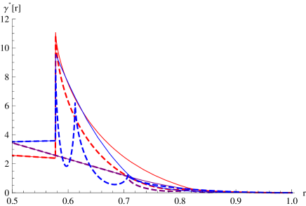
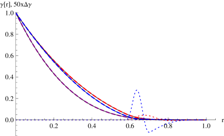
Figure 1: Top panel: the continuous curves represent the exact CLD of the cube (red), the octahedron (blue) and the tetrahedron (purple). The corresponding algebraic approximations, of order $K=0$, are represented by the dashed curves with the same colours. Bottom panel: the resulting approximations of the associated CFs are represented with the same colours. The thin black lines, hardly distinguishable from the dashed ones, refer to the exact CFs. The dotted curves are the errors (multiplied by 50).

This conclusion is further strenghtned by the top panel of Fig. 2 which shows $I(q)$ versus $q$, i.e.  the 3D Fourier transforms (FT) of the exact and the approximated CFs. The agreement appears to be quite good throughout the reported tange of the scattering vector, denoted by $Q$, (instead of $q$) in the figures. We recall the sum-rule (Guinier& Fournet, 1955; Feigin & Svergun, 1987): $I(0)=\int_{R^{3}}\gamma(r)dv=V$ where $V$ denotes the particle volume. From this and the fact that the approximated and the exact FTs, for each particle shape, practically coincide at $q=0$, we conclude that the approximated CFs fairly obey the sum-rule.

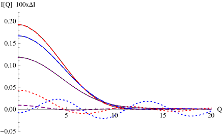
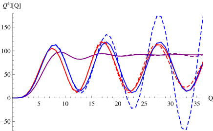
Figure 2: Top panel: the exact and the approximated form factors of the three considered particle shapes, are given by the thin continuous black curves and the closer coloured broken ones. They practically coincide. [The colours depend on the particle shape as specified in the Fig.1 caption.] The dashed curves are obtained by the 3D Fourier transform of the (K=0) CF approximations. The errors, multiplied by 100, are shown, with the same colours, by the dotted curves oscillating around the horizonatal axis. Bottom panel: Porod plot of the intensities resulting from the FTs of the exact (continuous) and the approximated (dashed) CFs.

However, the Porod plot is a tool much more accurate to evaluate the accuracy of an approximation. The bottom panel shows the Porod plots of the considered approximations. One sees that the scattering intensities relevant to the CF approximations of the tetrahedron and the cube are accurate throughout the reported $q$-range, while that of the octahedron is only accurate up to $q\approx 10$. In the three cases, however, one notes that the accuracy deteriorates as $q$ increases. This is by no way surprising because the $K=0$ approximations of the CLDs only reproduces the first-order discontinuities (Ciccariello, 1985) of the exact CLDs. The CLDs’ higher order derivatives show further singularities [see Ciccariello (205b, 2014b)] that are responsible for further damped oscillatory contributions in the Porod plots. Besides, the CLD approximations, shown in Fig. 1, show artificial wells that, by Fourier transforming, yield peaks around $q=2\pi/\delta$ with $\delta$ equal to the positions of the minima of the wells. Only beyond the largest of these $q$ values, the approximated and the exact Porod plots are expected to coincide and the noted discrepancies to disappear.

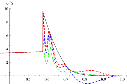
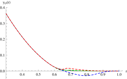
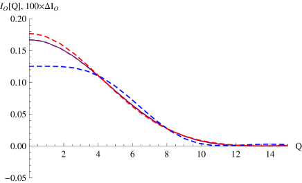
Figure 3: Top panel: the thin black curve is the exact CLD and the broken green, blue and red curves respectively represent the CLD approximations relevant to $K=0$, $K=1$ and $K=2$. Middle panel: with the same colours we plot the CF approximations resulting from the above CLD approximations. Bottom panel: plots of the scattering intensities relevant to the three approximations in the inner $q$-range.

Fig. 3 allows us to appreciate how things change as we increase the approximation order. It refers to the only octahedron which has a CLD more structured than the tetrahedron’s and the cube’s. The top panel shows that, as $K$ increases from 0 to 2, the approximated CLD becomes, so to speak, more adherent to the exact one around the end points of the distance subintervals. In the two internal subintervals, the approximated CLD gets nearer to the exact one throughout the full subintervals, while in outer one it gets farther as we pass from $K=0$ to $K=1$ and then closer for $K=2$, remaining however farther than the $K=0$ approximation. This last discrepancy propagates towards the inner two subintervals owing to the matching procedure so that the final accuracy of the total CF approximation worsens as we pass from $K=0$ to $K=2$ and to $K=1$, as it appears in the middle panel. This is confirmed by the bottom panel that shows the corresponding scattering intensity in the innermost $q$-range. The improvement of the approximations as $K$ increases can only be appreciated by the corresponding Porod plots that are reported in the ms’ part deposited with IUCr. There it appears that the $K=1$ and $K=2$ intensities almost coincide with the exact one in the region $q>500$, while we must go beyond $q=3000$ for this to happen for the $K=0$ approximation.

4 - Conclusions
From the above results it appears reasonable to conclude that the simplest approximation, relevant to the choice $K=0$, yields an algebraic approximation of the CF accurate enough to meet the standards of crystallographers and small-angle scattering people. We conclude with two remarks. First, the reported procedure still works if the value of $K$ is differently chosen in the different subintervals. For instance, the behaviour of the CLD approximations, shown in Fig. 2, suggests that the choice $K=2$ in the second and third subinterval and $K=0$ in the fourth ought to be more accurate because the resulting approximation is closer to the exact CLD. Second, in constructing the CF approximation, the crucial point is that the approximation must continuously interpolates, together with its derivatives, the truncated expansions of the CLD at the end-points of the the considered subinterval. We have illustrated a procedure that achieves the aim, but other procedures are possible. For instance, taking advantage of the fact that the approximation error reduces with the subinterval lenghts, one could divide each subinterval into three parts, approximate the CLD with its left and right truncated expansions in the first and the third of these intervals, then continuously interpolate the truncated expansions, evaluated at the dividing points, by the above explained procedure and, finally, get the full CF algebraic approximations by the matching procedure. The paid cost is the greater complexity of the approximation.

Acknowledgments
I gratefully thank the anonymous referee for having raised the question of the possibility of approximating the CF starting from the CLD knowledge.

References

Ciccariello, S. (1985). Acta Cryst. A41, 560-568.

Ciccariello, S. (2005a). J. Appl. Cryst. 38, 97-106.

Ciccariello, S. (2005b). Fibres & Text. East Eur. 13, 41-46.

Ciccariello, S. (2014a). J. Appl. Cryst. 47, 1216-1227.

Ciccariello, S. (2014b). J. Appl. Cryst. 47, 1445-1448.

Ciccariello, S. (2020a). arXiv:1911.02532v2 [math-ph].

Ciccariello, S. (2020b). Acta Cryst. A76, https://doi.org/10.1107/S2053273320004519.

Ciccariello, S., Cocco, G., Benedetti, A. & Enzo, S. (1981). Phys. Rev. B23, 6474-6485.

Ciccariello, S. & Sobry, R. (1995). Acta. Cryst. A51, 60-69.

Erdéliy, A. (1956). Asymptotic Expansions, ch. II. New York:Dover.

Feigin, L.A. & Svergun, D.I. (1987). Structure Analysis by Small-Angle X-Ray and Neutron Scattering, New York: Plenum Press.

Goodisman, J. (1980). J. Appl. Cryst. 13, 132-134.

Guinier, A. & Fournet, G. (1955). Sall-Angle Scattering of X-rays, New York: John Wiley.