Data-driven Optimal Control of
a SEIR model for COVID-19

Abstract.

We present a data-driven optimal control approach which integrates the reported partial data with the epidemic dynamics for COVID-19. We use a basic Susceptible-Exposed-Infectious-Recovered (SEIR) model, the model parameters are time-varying and learned from the data. This approach serves to forecast the evolution of the outbreak over a relatively short time period and provide scheduled controls of the epidemic. We provide efficient numerical algorithms based on a generalized Pontryagin Maximum Principle associated with the optimal control theory. Numerical experiments demonstrate the effective performance of the proposed model and its numerical approximations.

1. Introduction

The outbreak of COVID-19 epidemic has resulted in over millions of confirmed and death cases, evoking fear locally and internationally. It has a huge impact on global economy as well as everyone’s daily life. Numerous mathematical models are being produced to forecast the spread of COVID-19 in the US and worldwide [3, 20, 9, 39]. These predictions have far-reaching consequences regarding how quickly and how strongly governments move to curb the epidemic. We aim to exploit the abundance of available data and integrate existing data with disease dynamics based on epidemiological knowledge.

One of the well-known dynamic models in epidemiology is the SIR model proposed by Kermack and McKendrick [32] in 1927. Here, $S,I,R$ represent the number of susceptible, infected and recovered people respectively. They use an ODE system to describe the transmission dynamics of infectious diseases among the population. In the current COVID-19 pandemic, actions such as travel restrictions, physical distancing and self-quarantine are taken to slow down the spread of the epidemic. Typically, there is a significant incubation period during which individuals have been infected but are not yet infectious themselves. During this period the individual is in compartment $E$ (for exposed), the resulting models are of SEIR or SEIRS type, respectively, depending on whether the acquired immunity is permanent or otherwise. Also such models can show how different public health interventions may affect the outcome of the epidemic, and can also predict future growth patterns.

Optimal control provides a perspective to study and understand the underlying transmission dynamics. The classical theory of optimal control was originally developed to deal with systems of controlled ordinary differential equations [24, 11]. Computational methods have been designed to solve related control problems [35, 16, 50]. There is a wide application to various fields, including those for epidemic models, with major control measures on medicine (vaccination), see e.g., [28, 7], and for Cancer immunotherapy control [13].

In this paper, we integrate the optimal control with a specific SEIR model, though the developed methods can be readily adapted to other epidemic ODE models. More precisely, we introduce a dynamic control model for monitoring the virus propagation. Here the goal is to advance our understanding of virus propagation by learning the model parameters so that the error between the reported cases and the solution to the SEIR model is minimized. In short, we formulate the following optimization problem

$$\min_{\theta}\quad J=\sum_{i=1}^{n-1}L(U(t_{i}))+g(U(T)),$$

s.t. $$\dot{U}=F(U,\theta)\quad t\in(0,T],\quad U(0)=U_{0},\quad\theta\in\Theta.$$

Here $\dot{U}=\frac{d}{dt}U(t)$, $\theta$ is a time-varying vector of model parameters, $\Theta$ is the admissible set for model parameters $\theta$, and $U=[S,E,I,R,D]^{\top}$ corresponds to the susceptible, exposed, infected, recovered and deceased population. The loss function $J$ is composed of two parts: $L$ measures the error between the candidate solution to the SEIR system and the reported data at intermediate observation times, and $g$ measures the error between the candidate solution and the scheduled control data at the end time. This is in contrast to the standard approach of fitting the model to the epidemic data through the non-linear least squares approach [3, 20, 9].

1.1. Main contributions

In the present work we provide a fairly complete modeling discussion on parameter learning, prediction and control of epidemics spread based on the SEIR model. We begin with our discussion of basic properties of the SEIR model. Then we show how the parameters can be updated recursively by gradient-based methods for a short time period while parameters are near constants, where the loss gradient can be obtained by using both state and co-state dynamics. For an extended time period with reported data available at intermediate observation times, the parameters are typically time-varying. In this general setting, we derive necessary conditions to achieve optimal control in terms of the chosen objectives. The conditions are essentially the classical Pontryagin maximum principal (PMP)[46]. The main differences are in the way we apply the principle in each time interval, and connect them consistently by re-setting the co-state $V$ at the end of each time interval. We thus named it the generalized PMP. We further present an algorithm to find the numerical solution to the generalized PMP in the spirit of the method of successive approximations (MSA)[16]. Our algorithm is mainly fulfilled by three parts: (1) discretization of the forward problem in such a way that solutions to $U$ remain positive for an arbitrarily step size $h$; (2) discretization of the co-state equation for $V$ is made unconditionally stable; (3) Minimiziation of the Hamiltonian is given explicitly based on the structure of the SEIR model.

This data-driven optimal control approach can be applied to other epidemic models. In particular, the prediction and control can be combined into one framework. To this end, the cost includes terms measuring the error between confirmed cases (infection and death) and those predicted from the model during the evolution, and terms measuring the error between the scheduled numbers as desired and those predicted from the model during the control period.

1.2. Further related work

In the mathematical study of SIR models, there is an interplay between the dynamics of the disease and that of the total population, see [4, 44, 22, 52]. We refer the reader to [41, 21] for references on SEIRS models with constant total population and to [38] for the proof of the global stability of a unique endemic equilibrium of a SEIR model. Global stability of the endemic equilibrium for the SEIR model with non-constant population is more subtle, see [37]. Apart from the compartmental models (and their stochastic counterparts [2]), a wide variety of methods exist for modeling infectious disease. These include diffusion models [12], mean-field-type models [33], cellular automata [56], agent-based models [27], network-based models [55, 30, 45], and game-theoretical modelling [6, 48, 14]. Some focus on the aggregate behaviour of the compartments of the population, whereas others focus on individual behaviour.

For COVID-19, a data-driven model has been proposed and simulated in [43], where both the SIR model and the feed-forward network are trained jointly. Compared to this work, our data-driven model is to consider the optimal control for SEIR with rigorous derivation of optimality conditions and stable numerical approximations. On the other hand, our data-driven optimal control algorithm may be interpreted as training a deep neural network in which the SEIR model serves as the neural network with parameters to be learned. This is in contrast to the study of residual neural networks using neural ODEs (see e.g., [19, 15]) or section dynamics [40]. For other works on data-driven learning model parameters using neural networks, see [5, 29]. SIR models with spatial effects have been studied [8, 36]. A SIRT model was proposed in [8] to study the effects of the presence of a road on the spatial propagation of the COVID-19. Introduced in [36] is a mean-field game algorithm for a spatial SIR model in controlling propagation of epidemics.

Finally, we would like to mention that a variety of works have sought to endow neural networks with physics-motivated equations, which can improve machine learning. To incorporate the equations, parametric approaches have been studied [23, 17, 42, 47], where certain terms in the equations are learned, while the equations still govern the dynamics from input to output.

1.3. Organization

In Section 2, we motivate and present the SEIR system for modelling the time evolution of epidemics, and integrate it with data into an optimal control system. Both algorithms and related numerical approximations are detailed in Section 3. Section 4 provides experimental results to show the performance of our data-driven optimal control algorithms. We end with concluding remarks in Section 5.

2. The SEIR model and optimal control

2.1. Model formulation

A population of size $N(t)$ is partitioned into subclasses of individuals who are susceptible, exposed (infected but not yet infectious), infectious, and recovered, with sizes denoted by $S(t),E(t),I(t),R(t)$, respectively. The sum $E+I$ is the total infected population.

The dynamical transfer of the population is governed by an ODE system

$$\dot{S}=A-\beta SI/N-dS,$$

$$\dot{E}=\beta SI/N-\epsilon E-dE,$$

$$\dot{I}=\epsilon E-\mu I-\gamma I-dI,$$

$$\dot{R}=\gamma I-dR,$$

$$\dot{D}=\mu I,$$ (2.1)

subject to initial conditions $S_{0},E_{0},I_{0},R_{0},D_{0}$. Here $D(t)$ denotes deaths at time $t$, $A$ denotes the recruitment rate of the population due to birth and immigration. It is assumed that all newborns are susceptible and vertical transmission can be neglected. $d$ is the natural death rate, $\mu$ is the rate for virus-related death. $\gamma$ is the rate for recovery with $1/\gamma$ being the mean infectious period, and $\epsilon$ is the rate at which the exposed individuals become infectious with $1/\epsilon$ being the mean incubation period. The recovered individuals are assumed to acquire permanent immunity (yet to be further confirmed for COVID-19); there is no transfer from the $R$ class back to the $S$ class. $\beta$ is the effective contact rate. In the limit when $\epsilon\to\infty$, the SEIR model becomes a SIR model. Note that the involved parameters do not correspond to the actual per day recovery and mortality rates as the new cases of recovered and deaths come from infected cases several days back in time. However, one can attempt to provide some coarse estimations of the “effective/apparent” values of these epidemiological parameters based on the reported confirmed cases.

2.2. Solution properties of the SEIR model

Classical disease transmission models typically have at most one endemic equilibrium. If there is no endemic equilibrium, diseases will disappear. Otherwise, the disease will be persistent irrespective of initial positions. Large outbreaks tend to the persistence of an endemic state and small outbreaks tend to the extinction of the diseases.

To understand solution properties of the SEIR system, we simply take $A=bN$ with $b$ the natural birth rate, and focus on the following sub-system

$$\dot{S}=bN-\beta SI/N-dS,$$

$$\dot{E}=\beta SI/N-\epsilon E-dE,$$

$$\dot{I}=\epsilon E-\mu I-\gamma I-dI,$$

$$\dot{R}=\gamma I-dR$$

with the total population size $N=S+E+I+R$. By adding the equations above we obtain

$$\dot{N}=(b-d)N-\mu I.$$

Let $s=S/N,e=E/N,i=I/N,r=R/N$ denote the fractions of the classes $S,E,I,R$ in the population, respectively, then one can verify that

$$\dot{s}=b-bs-\beta is+\mu is,$$ (2.2a)

$$\dot{e}=\beta is-(\epsilon+b)e+\mu ie,$$ (2.2b)

$$\dot{i}=\epsilon e-(\mu+\gamma+b)i+\mu i^{2},$$ (2.2c)

where $r$ can be obtained from $r=1-s-e-i$ or

$$\dot{r}=\gamma i-br+\mu ir.$$

From biological considerations, we study system (2.2) in a feasible region

$$\Sigma=\{(s,e,i)\in\mathbb{R}^{3}_{+},0\leq s+e+i\leq 1\}.$$

It can be verified that $\Sigma$ is positively invariant with respect to the underlying dynamic system. We denote $\partial\Sigma$ and $\Sigma^{0}$ the boundary and the interior of $\Sigma$ in $\mathbb{R}^{3}$, respectively. A special solution of form $P^{0}=(1,0,0)$ on the boundary of $\Sigma$ is the disease-free equilibrium of system (2.2) and it exists for all non-negative values of its parameters. Any equilibrium in the interior $\Sigma^{0}$ of $\Sigma$ corresponds to the disease being endemic and is named an endemic equilibrium. To identify the critical threshold for the parameters, we take $\epsilon\times$(2.2b)+ $(\epsilon+b)\times$(2.2c) to obtain

$$\frac{d}{dt}[\epsilon e+(\epsilon+b)i] =i\left[\epsilon\beta s+\epsilon\mu e+\mu(\epsilon+b)i-(\epsilon+b)(\gamma+\mu+b)\right]$$

$$\leq i\left[\max\{\epsilon\beta,\epsilon\mu,\mu(\epsilon+b)\}-(\epsilon+b)(\gamma+\mu+b)\right]\leq 0,$$

provided a key quantity $\sigma\leq 1$, where

$$\sigma:=\frac{\beta\epsilon}{(\epsilon+b)(\gamma+\mu+b)}$$

is called the modified contact number [37]. The global stability of $P^{0}$ when $\sigma\leq 1$ follows from LaSalle’s invariance principle. The following theorem (see [37]), a standard type in mathematical epidemiology, shows that the basic number $\sigma$ determines the long-term outcome of the epidemic outbreak.

Theorem 2.1.

1. If $\sigma\leq 1$, then $P^{0}$ is the unique equilibrium and globally stable in $\Sigma$.
2. If $\sigma>1$, then $P^{0}$ is unstable and the system is uniformly persistent in $\Sigma^{0}$.

By this theorem, the disease-free equilibrium $P^{0}$ is globally stable in $\Sigma$ if and only if $\sigma\leq 1$. Its epidemiological implication is that the infected fraction of the population vanishes in time so the disease dies out. In addition, the number $\sigma$ serves as a sharp threshold parameter; if $\sigma>1$, the disease remains endemic.

In the epidemic literature, another threshold quantity is the basic reproduction number

$$R_{0}=\frac{\beta}{\gamma+\mu},$$

which is the product of the contact rate $\beta$ and the average infectious period $\frac{1}{\gamma+\mu}$. It is a parameter well known for quantifying the epidemic spread [18, 54]. On the other hand, the contact number $\sigma$ is defined at all times. In general, we have

$$R_{0}\geq\sigma.$$

Note that for most models, $\sigma=R_{0}$, both quantities can be used interchangeably. This is the case in our experiments when taking $b=0$.

Remark 2.2.

Extensive evidence shows that the disease spread rate is sensitive to at least three factors: (1) daily interactions, (2) probability of infection, and (3) duration of illness. The above assertion shows that making efforts to decrease $R_{0}$ is essential for controlling propagation of epidemics. Hence measures such as social distancing (self-quarantine, physical separation), washing hands and wearing face coverings, as well as testing / timely-hospitalization can collectively decrease $R_{0}$.

Remark 2.3.

The above model if further simplified will reduce to the SIR model or SIS model, which is easier to analyze [25, 10, 53]. It can also be enriched by dividing into different groups [34, 51], or by considering the spatial movement effects [26, 31]. In this work, we use the SEIR model as a base for our analysis, prediction, and control.

2.3. A simple control

In compact form, the SEIR system may be written as

$$\dot{U}=F(U;\theta),\quad U(0) =U_{0},$$

where

$$U=[S,E,I,R,D]^{\top},\quad\theta=[\beta,\epsilon,\gamma,\mu]^{\top}$$

are the column vectors of the state and parameters, respectively. Let $g(\cdot)$ be a loss function (to be specified later) at the final time $T$, then the problem of determining the model parameters based on this final cost can be cast as a dynamic control problem:

$${\rm min}_{\theta}\{g(U(T))\quad\hbox{subject to }\;\;\dot{U}=F(U,\theta),\quad 0<t\leq T;\quad U(0)=U_{0};\quad\theta\in\Theta\}.$$

Here the dependence of $g$ on $\theta$ is through $U(T)$. The set of admissible parameters $\Theta$ may be estimated from other sources.

For a short time period, the model parameters are near constant, then we can use gradient-based methods to directly update $\theta$, for which $\nabla_{\theta}g$ needs to be evaluated. We define the Lagrangian functional

$$\mathcal{L}(\theta) =g(U(T))-\int_{0}^{T}(\dot{U}-F(U,\theta))^{\top}Vdt,$$

where $V=V(t)$ is the Lagrangian multiplier depending on time and can be chosen freely, and $U$ depends on $\theta$ through the ODE. A formal calculation gives

$$\nabla_{\theta}g =\nabla_{\theta}\mathcal{L}$$

$$=(\nabla_{\theta}U(T))^{\top}\nabla_{U}g+\int_{0}^{T}\left((\nabla_{U}F)(\nabla_{\theta}U(t))+\nabla_{\theta}F-\nabla_{\theta}\dot{U}(t)\right)^{\top}V(t)dt$$

$$=(\nabla_{\theta}U(T))^{\top}\left(\nabla_{U}g-V(T)\right)+(\nabla_{\theta}U(0))^{\top}V(0)$$

$$\qquad+\int_{0}^{T}(\nabla_{\theta}U(t))^{\top}\left((\nabla_{U}F)^{\top}V(t)+\dot{V}(t)\right)+(\nabla_{\theta}F)^{\top}V(t)dt.$$

Thus $\nabla_{\theta}g$ can be determined in the following steps:

• Solve the forward problem for state $U$,

  $$\dot{U}(t)=F(U(t),\theta),\quad U(0)=U_{0}.$$

• Solve the backward problem for co-state $V$,

  $$\dot{V}(t)=-(\nabla_{U}F)^{\top}V(t),\quad V(T)=\nabla_{U}g(U(T)).$$

• Evaluate the gradient of $g$ by

  $$\nabla_{\theta}g=\int_{0}^{T}(\nabla_{\theta}F)^{\top}V(t)dt.$$

In the context of the optimal control theory [46], such $V$ exists and is called the co-state function. We note that the $(U,V)$ dynamical system models the optimal strategies for $S,E,I,R$ populations.

Remark 2.4.

It is remarkable that computing gradients of a scalar-valued loss with respect to all parameters is done using only state and co-state functions without backpropagating through the operations of the solver. In addition, modern ODE solvers may be used to compute both $U$ and $V$.

2.4. Data-driven optimal control

Now we consider an extended time period with reported data available at intermediate observation times. The data are taken from the reported cumulative infection and death cases. In such general case the parameters are typically time-varying, we need to derive a more refined data-driven optimal control. Arranging the data in a vector $U_{c}=[I_{c},D_{c}]^{\top}$ at times $0=t_{0}<t_{1}<t_{2}<...<t_{n}=T$, we aim to

• find optimal parameter $\theta(t)$ for $0\leq t\leq t_{n-1}$ such that the solution to the SEIR system fits the reported data at the grid points $\{t_{i}\}_{i=1}^{n-1}$ as close as possible, and

• find desired parameter $\theta(t)$ for $t_{n-1}\leq t\leq T$ that is able to control the epidemic spreading at time $T$ at desired values.

To achieve these goals, we first define a loss function by

$$J=\sum_{i=1}^{n-1}L(U(t_{i}))+g(U(T)),$$

where

$$L(U(t_{i})) =\lambda_{1}|I(t_{i})-I_{c}(t_{i})|^{2}+\lambda_{2}|D(t_{i})-D_{c}(t_{i})|^{2},\quad 1\leq i\leq n-1,$$ (2.3)

$$g(U(T)) =\lambda_{1}|I(T)-I_{d}(T)|^{2}+\lambda_{2}|D(T)-D_{d}(T)|^{2}.$$

Here $\lambda_{1},\lambda_{2}$ are user-defined normalization factors. This loss function is composed of two parts: the running cost $L$ which measures the error between the candidate solution $(I,D)$ to the SEIR system and the reported data $(I_{c},D_{c})$ at intermediate times; and the final cost $g$, which measures the error between the candidate solution $(I,D)$ and the desired data $(I_{d},D_{d})$ at the end time.

We then formulate the task as the following optimal control problem

$$\min J=\sum_{i=1}^{n-1}L(U(t_{i}))+g(U(T)),$$ (2.4)

s.t. $$\dot{U}=F(U,\theta)\quad t\in(0,T],\quad U(0)=U_{0},\quad\theta\in\Theta.$$

Motivated by the classical optimal control theory, we derive the necessary conditions for the optimal solution to problem (2.4), stated in the following theorem.

Theorem 2.5.

Let $\theta^{*}$ be the optimal solution to problem (2.4) and $U^{*}$ be the corresponding state function, then there exists a piece-wise smooth function $V^{*}$ and a Hamiltonian $H$ defined by

$$H(U,V,\theta)=V^{\top}F(U,\theta)$$ (2.5)

such that

$$\dot{U^{*}}=F(U^{*},\theta^{*}),\quad t\in(0,T],\quad U^{*}(0)=U_{0},$$ (2.6)

$$\dot{V^{*}} =-(\nabla_{U}F(U^{*},\theta^{*}))^{\top}V,\quad t_{i-1}\leq t<t_{i},\quad i=n,...,1,$$ (2.7)

$$V^{*}(T) =\nabla_{U}g(U^{*}(T)),$$

$$V^{*}(t_{i}^{-}) =V^{*}(t_{i}^{+})+\nabla_{U}L(U^{*}(t_{i})),\quad i=n-1,...,1$$

are satisfied. Moreover, the Hamiltonian minimization condition

$$H(U^{*},V^{*},\theta^{*})\leq H(U^{*},V^{*},a)\quad\forall a\in\Theta$$

holds for all time $t\in[0,T]$ but $\{t_{i}\}_{i=1}^{n-1}$.

Proof.

Recall the classical Bolza optimal control problem [11]

$$\min\quad J=\int_{0}^{T}L(U(t),\theta(t))dt+g(U(T))$$

s.t. $$\dot{U}=F(U,\theta),\quad t\in[0,T],\quad U(0)=U_{0},\quad\theta(t)\in\Theta.$$

The Pontryagin’s maximum principle states the necessary conditions for optimality: assume $\theta^{*}$ and $U^{*}$ are the optimal control function and corresponding state of the system, then there exists a function $V^{*}$ and a Hamiltonian $H$ defined for all $t\in[0,T]$ by

$$H(U,V,\theta)=V^{T}F(U,\theta)+L(U,\theta)$$

such that

$$\dot{U^{*}} =\nabla_{V}H(U^{*},V^{*},\theta^{*}),\quad U^{*}(0)=U_{0},$$ (2.8)

$$\dot{V^{*}} =-\nabla_{U}H(U^{*},V^{*},\theta^{*}),\quad V^{*}(T)=\nabla_{U}g(U^{*}(T)),$$ (2.9)

are satisfied. Moreover, the Hamiltonian minimization condition

$$H(U^{*},V^{*},\theta^{*})\leq H(U^{*},V^{*},a)$$

holds for all time $t\in[0,T]$ and for all permissible control function $a\in\Theta$.

Notice that the loss function in (2.4) can be rewritten as

$$J=\int_{0}^{T}\sum_{i=1}^{n-1}L(U(t))\delta(t-t_{i})dt+g(U(T)),$$

where $\delta(x)$ is the Dirac delta function, then the corresponding Hamiltonian reads as

$$H(U,V,\theta)=V^{T}F(U,\theta)+\sum_{i=1}^{n-1}L(U(t))\delta(t-t_{i}).$$ (2.10)

Hence (2.8) can be expressed as (2.6), (2.9) has the form of

$$\dot{V}=-\sum_{i=1}^{n-1}\nabla_{U}L(U(t))\delta(t-t_{i})-(\nabla_{U}F(U,\theta))^{\top}V,\quad V(T)=\nabla_{U}g(U(T)).$$ (2.11)

Integrate (2.11) from $t^{-}_{i}-\epsilon$ to $t^{+}_{i}+\epsilon$ and let $\epsilon$ goes to $0$, then for $i=n-1,...,1$

$$V(t^{+}_{i})-V(t^{-}_{i})=\nabla_{U}L(U(t_{i})).$$

Thus in each interval, (2.11) reduces to

$$\dot{V}=-(\nabla_{U}F(U,\theta))^{\top}V,\quad t_{i-1}\leq t<t_{i},\quad i=n,...,1,$$

which is exactly (2.7). Correspondingly, the Hamiltonian (2.10) reduces to (2.5) for all $t\in[0,T]$ but $\{t_{i}\}_{i=1}^{n-1}$. ∎

3. Numerical discretization and algorithms

In this section, we present implementation details to solve problem (2.4) via solving the generalized PMP by iteration. We proceed in the following manner. First we make an initial guess $\theta_{0}\in\Theta$. From the control function $\theta_{l}(t)$ in the $l$-th iteration for $l=0,1,2,\cdots$, we obtain $\theta_{l+1}(t)$ in three steps:
Step 1: Solve the forward problem (2.6) to obtain $U_{l}$.
Step 2: Solve the sequence of backward problems (2.7) to obtain $V_{l}$.
Step 3: $\theta_{l+1}=\operatorname*{arg\!\min}_{\theta\in\Theta}H(U_{l},V_{l},\theta,t)$ for each $t\in[0,T]$.

This is essentially the method of successive approximations (MSA) [16]. An important feature of MSA is that the Hamiltonian minimization step is decoupled for each $t$. However, in general MSA tends to diverge, especially if the bad initial guess is taken [16].

Our goal is to adopt a careful discretization at each step to control possible divergent behavior, instead of simply call an existing ODE solver for Steps 1-2, and an optimization algorithm for Step 3.

Within each interval $(t_{i-1},t_{i})$, we approximate both $U$ and $V$ at the same $m$ points with step size $h=(t_{i}-t_{i-1})/m$, so that the value of $U$ required in Step 2 are already calculated in Step 1. We use $U^{i,k},V^{i,k},\theta^{i,k}$, where $i=1,...,n$ and $k=0,...,m$ to denote solution values at $k$-th point in the $i$-th interval.

Note that population dynamics (births or deaths) may be neglected at a very crude level on the grounds that epidemic dynamics often occur on a faster time scale than host demography, or we can say heuristically that death of an infected individual and subsequent replacement by a susceptible (in the absence of vertical transmission) is equivalent to a recovery event. Hence, in the numerical study, both $b$ and $d$ are taken to be zero.

Below we discuss the discretization of the three iteration steps for the case $b=d=0$.

3.1. Forward discretization

We focus on the time interval $(t_{i-1},t_{i})$. For notation simplicity, we use $U^{k},V^{k},\theta^{k}$ to represent corresponding values at the $k$-th point. We discretize the forward problem (2.6) by an explicit-implicit method with the Gauss-Seidel type update:

$$\frac{S^{k+1}-S^{k}}{h} =-\beta^{k}S^{k+1}I^{k}/N^{k},$$

$$\frac{E^{k+1}-E^{k}}{h} =\beta^{k}S^{k+1}I^{k}/N^{k}-\epsilon^{k}E^{k+1},$$

$$\frac{I^{k+1}-I^{k}}{h} =\epsilon^{k}E^{k+1}-(\gamma^{k}+\mu^{k})I^{k+1},$$

$$\frac{R^{k+1}-R^{k}}{h} =\gamma^{k}I^{k+1},$$

$$\frac{D^{k+1}-D^{k}}{h} =\mu^{k}I^{k+1}.$$

This gives

$$S^{k+1} =\frac{S^{k}}{1+h\beta^{k}I^{k}/N^{k}},$$ (3.1)

$$E^{k+1} =\frac{E^{k}+h\beta^{k}S^{k+1}I^{k}/N^{k}}{1+h\epsilon^{k}},$$

$$I^{k+1} =\frac{I^{k}+h\epsilon^{k}E^{k+1}}{1+h(\gamma^{k}+\mu^{k})},$$

$$R^{k+1} =R^{k}+h\gamma^{k}I^{k+1},$$

$$D^{k+1} =D^{k}+h\mu^{k}I^{k+1},$$

where $k=0,1,...,m-1$, $h=(t_{i}-t_{i-1})/m$ is the step size. The most important property of this update is its unconditional positivity-preserving property, i.e,

$$U^{k}\geq 0\Rightarrow U^{k+1}>0,\;k=0,\cdots$$

irrespective of the size of the step size $h$. For the starting value in each interval, we have

$$U^{1,0}=U(0),\quad U^{i,0}=U^{i-1,m},\quad i=2,\cdots,n-1.$$

3.2. Backward discretization

Let $V=[V_{S},V_{E},V_{I},V_{R},V_{D}]^{\top}$ and notice that

$$\nabla_{U}F=\begin{bmatrix}-\beta I(N-S)/N^{2}&0&-\beta S(N-I)/N^{2}&0&0\\ \beta I(N-S)/N^{2}&-\epsilon&\beta S(N-I)/N^{2}&0&0\\ 0&\epsilon&-(\mu+\gamma)&0&0\\ 0&0&\gamma&0&0\\ 0&0&\mu&0&0\end{bmatrix},$$

then (2.7) takes the following form

$$\dot{V_{S}} =\beta I(N-S)(V_{S}-V_{E})/N^{2},$$

$$\dot{V_{E}} =\epsilon(V_{E}-V_{I}),$$

$$\dot{V_{I}} =\beta S(N-I)(V_{S}-V_{E})/N^{2}+\gamma(V_{I}-V_{R})+\mu(V_{I}-V_{D}),$$

$$\dot{V_{R}} =\dot{V_{D}}=0.$$

In a similar fashion to the discretization of $U$, we discretize this system by an explicit-implicit method by

$$\frac{V^{k+1}_{S}-V^{k}_{S}}{h} =\beta^{k}I^{k}(N^{k}-S^{k})(V_{S}^{k}-V_{E}^{k+1})/(N^{k})^{2},$$

$$\frac{V^{k+1}_{E}-V^{k}_{E}}{h} =\epsilon^{k}(V_{E}^{k}-V_{I}^{k+1}),$$

$$\frac{V^{k+1}_{I}-V^{k}_{I}}{h} =\beta^{k}S^{k}(N^{k}-I^{k})(V_{S}^{k}-V_{E}^{k})/(N^{k})^{2}+\gamma^{k}(V^{k}_{I}-V^{k+1}_{R})+\mu^{k}(V^{k}_{I}-V^{k+1}_{D}),$$

$$V^{k}_{R} =V^{k+1}_{R},\qquad V^{k}_{D}=V^{k+1}_{D}.$$

Then the scheme is given by

$$V^{k}_{S} =\frac{V^{k+1}_{S}(N^{k})^{2}+h\beta^{k}I^{k}(N^{k}-S^{k})V^{k+1}_{E}}{(N^{k})^{2}+h\beta^{k}I^{k}(N^{k}-S^{k})},$$ (3.2)

$$V^{k}_{E} =\frac{V^{k+1}_{E}+h\epsilon^{k}V^{k+1}_{I}}{1+h\epsilon^{k}},$$

$$V^{k}_{I} =\frac{V^{k+1}_{I}+h\left(\gamma^{k}V_{R}+\mu^{k}V_{D}-\beta^{k}S^{k}(N^{k}-I^{k})(V_{S}^{k}-V_{E}^{k})/(N^{k})^{2}\right)}{1+h(\gamma^{k}+\mu^{k})},$$

$$V^{k}_{R} =V^{k+1}_{R},\qquad V^{k}_{D}=V^{k+1}_{D},$$

where $k=m-1,...,0$, $h=(t_{i}-t_{i-1})/m$ is the step size. For the starting value in each interval, we have

$$V^{n,m}=\nabla_{U}g(U(T)),\quad V^{i,m}=V^{i+1,0}+\nabla_{U}L(U(t_{i})),\quad i=n-1,\cdots,1.$$

Note that the above discretization is well-defined for any $h>0$, hence unconditionally stable since the system is linear in $V$.

3.3. Hamiltonian minimization

The Hamiltonian (2.5) is given by

$$H(U,V,\theta)=-V_{S}\beta SI/N+V_{E}(\beta SI/N-\epsilon E)+V_{I}(\epsilon E-(\gamma+\mu)I)+V_{R}\gamma I+V_{D}\mu I.$$

After plugging in $U(t),V(t)$ that is obtained by solving the above forward and backward problems with given $\theta(t)$, $H$ may be seen as a functional only with respect to $\theta$. We solve it by the proximal point algorithm (PPA) [49], that is for any fixed time $t\in(t_{i-1},t_{i})$, $i=1,2,...,n,$

$$\theta_{l+1}(t)=\operatorname*{arg\!\min}_{\theta(t)\in\Theta}\left\{H(U_{l}(t),V_{l}(t),\theta(t))+\frac{1}{2\tau}\|\theta(t)-\theta_{l}(t)\|^{2}\right\},$$ (3.3)

where $l$ is the index for iteration, $\tau$ is the step size.

Remark 3.1.

The use of PPA brings two benefits: (1) the objective function in (3.3) is a convex function, which ensures the existence of the solution to the minimization problem; (2) it is numerically stable: PPA has the advantage of being monotonically decreasing, which is guaranteed for any step size $\tau>0$. In this way, the convergence of minimizing the original loss in (2.4) with a regularization term is ensured, hence address the convergence issue that MSA generally has [1].

Given discretized $U^{\alpha}$ and $V^{\alpha}$ with $\alpha=\{i,k\}$, we solve (3.3) on grid points, that is to solve

$$\theta^{\alpha}_{l+1}=\operatorname*{arg\!\min}_{\theta\in\Theta}\left\{H(U^{\alpha}_{l},V^{\alpha}_{l},\theta)+\frac{1}{2\tau}\|\theta-\theta^{\alpha}_{l}\|^{2}\right\}.$$ (3.4)

Since $H$ is smooth, the above formulation when the constraint is not imposed is equivalent to the following

$$\theta^{\alpha}_{l+1}=\theta^{\alpha}_{l}-\tau\nabla_{\theta}{H}(U^{\alpha}_{l},V^{\alpha}_{l},\theta^{\alpha}_{l+1}).$$

The special form of $H$ allows us to obtain a closed form solution:

$$\beta^{\alpha}_{l+1} =\beta^{\alpha}_{l}+\tau S^{\alpha}_{l}I^{\alpha}_{l}((V_{S})^{\alpha}_{l}-(V_{E})^{\alpha}_{l})/N^{\alpha}_{l},$$ (3.5)

$$\epsilon^{\alpha}_{l+1} =\epsilon^{\alpha}_{l}+\tau E^{\alpha}_{l}((V_{E})^{\alpha}_{l}-(V_{I})^{\alpha}_{l}),$$

$$\gamma^{\alpha}_{l+1} =\gamma^{\alpha}_{l}+\tau I^{\alpha}_{l}((V_{I})^{\alpha}_{l}-(V_{R})^{\alpha}_{l}),$$

$$\mu^{\alpha}_{l+1} =\mu^{\alpha}_{l}+\tau I^{\alpha}_{l}((V_{I})^{\alpha}_{l}-(V_{D})^{\alpha}_{l}).$$

Now taking the constraint $\theta\in\Theta$ into consideration, we simply project the solution (3.5) back into the feasible region after each iteration, that is

$$\theta^{\alpha}_{l+1}=clip(\theta^{\alpha}_{l+1},\underline{\Theta},\overline{\Theta})$$

where $\underline{\Theta}$, $\overline{\Theta}$ are element-wise lower bound and upper bound of $\Theta$, respectively. That guarantees the output is constrained to be in $\Theta$.

Remark 3.2.

The step size for each parameter may be set differently according to their magnitude scale, and this can indeed improve the training performance, as observed in our experiments.

3.4. Algorithms

The above computing process is wrapped up in Algorithm 1. Since we can update $\{\theta^{i,k}\}$ simultaneously, we consider $\{\theta^{i,k}\}$ as a vector and still denote it as $\theta$ for notation simplicity. We use $\|\cdot\|$ to stand for the $L_{2}$ norm.

Algorithm 1

1:$\{U_{c}(t_{i})\}_{i=1}^{n}$: data, $t_{n}=T$: final time, $U_{0}$: initial data at $0$, $\theta_{0}$: initial guess, $\tau$: step size for the minimization problem

2:while $\|\theta_{l}-\theta_{l-1}\|/\|\theta_{l-1}\|>$ Tol do

3:     for $i=1$ to $n$ do

4:         for $k=0$ to $m-1$ do

5:              $U^{i,k+1}\leftarrow U^{i,k}$ (solve the forward problem, refer to (3.1))          

6:         $U^{i,0}\leftarrow U^{i-1,m}$ (update the initial condition for ODE solver)      

7:     $V^{n,m}\leftarrow\partial_{U}g(U(T))$ (set the initial data for the backward problem)

8:     for $i=n$ to $1$ do

9:         for $k=m-1$ to $0$ do

10:              $V^{i,k}\leftarrow V^{i,k+1}$ (solve the backward problem, refer to (3.2))          

11:         $V^{i,m}\leftarrow V^{i+1,0}+\partial_{U}L(U(t_{i}))$ (update the initial condition for ODE solver)      

12:     $\theta_{l+1}\leftarrow\theta_{l}$ (solve the minimization problem, refer to (3.5))

13:     $\theta_{l+1}\leftarrow clip(\theta_{l+1},\underline{\Theta},\overline{\Theta})$ (ensure $\theta\in\Theta$)

14:return $\theta,U$

This data-driven optimal control algorithm provides an optimal fitting to both the data and the SEIR model, it can help to reduce the uncertainty in conventional model predictions with standard data fitting.

Initialization: We now discuss how to initialize the control function $\theta$. A simple choice is to take $\theta_{0}^{i,k}$ to be a constant vector for all $1\leq i\leq n,1\leq k\leq m$, where the value of each component relies on a priori epidemiological and clinical information about the relative parameter magnitude. They vary with the area from where the data were sampled.

We can also use the data $\{D_{c}(t_{i})\}_{i=0}^{n},\{I_{c}(t_{i})\}_{i=0}^{n}$ to obtain a better initial guess for $\mu$. More precisely, from (2.1), i.e., $\mu=\dot{D}/I$ we take

$$\mu^{i,k}_{0}=\frac{D_{c}(t_{i+1})-D_{c}(t_{i})}{(t_{i+1}-t_{i})I_{c}(t_{i+1})}\quad\forall k=0,1,...,m.$$

The initial data for the forward problem is set as

$$U_{0}=[N(0)-I_{c}(0),0,I_{c}(0),0,D_{c}(0)]^{\top},$$

where $N(0)$ is the initial population of the area analyzed, $I_{c}(0)$, $D_{c}(0)$ are the confirmed infections and deaths on the day of the first confirmed cases, respectively.

The initial condition of the backward problem is given in (2.7). In the present setup, the loss function $g$ only depends on $I$ and $D$, hence the initial condition is given by

$$V^{n,m}=[0,0,\partial_{I}g(U(T)),0,\partial_{D}g(U(T))]^{\top}.$$

Finally, we should point out that Algorithm 1 with a rough initial guess $\theta_{0}$ can be rather inefficient when $T$ is large. In such case, we divide the whole interval as $0=t_{n_{0}}<t_{n_{1}}<...<t_{n_{s}}<t_{n_{s+1}}=T$ with $t_{n_{j}}\in\{t_{i}\}_{i=1}^{n-1}$ for $1\leq j\leq s$ and apply Algorithm 1 to each subinterval consecutively. This treatment is summarized in Algorithm 2.

Algorithm 2

1:$\{U_{c}(t_{i})\}_{i=1}^{n}$, $U_{0}$: initial data, $\tau$: step size for the minimization problem.

2:$\{t_{n_{j}}\}_{j=0}^{s+1}$, $\theta_{0}$: initial guess of $\theta$ on $[t_{n_{0}},t_{n_{1}}]$

3:for $j=0$ to $s$ do

4:     $\theta,U$ = Algorithm 1($\{U_{c}(t_{i})\}_{i=n_{j}+1}^{n_{j+1}}$, $[t_{n_{j}},t_{n_{j+1}}]$, $U_{0}$, $\theta_{0}$, $\tau$)

5:     $\theta_{0},U_{0}\leftarrow\theta(t_{n_{j+1}}),U(t_{n_{j+1}})$

6:     return $\theta,U$

Remark 3.3.

If parameters vary dramatically, $\theta(t_{n_{j}})$ may not be a good initialization for $\theta$ on $[t_{n_{j}},t_{n_{j+1}}]$. When this happens we switch to the rough initial guess and test by trial and error.

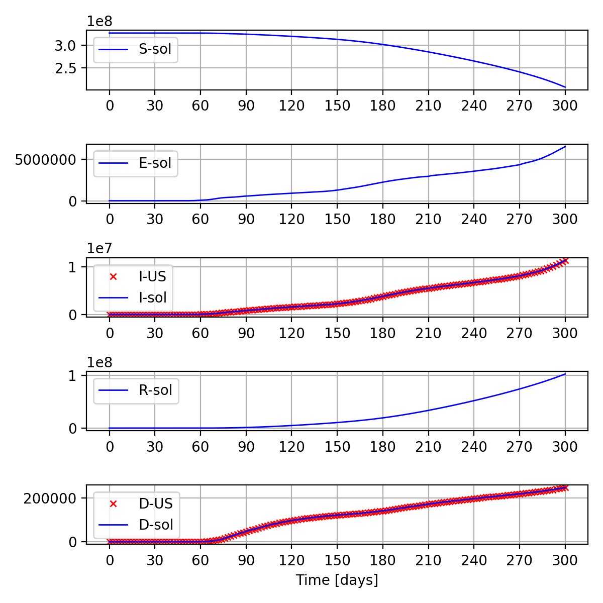
(a)

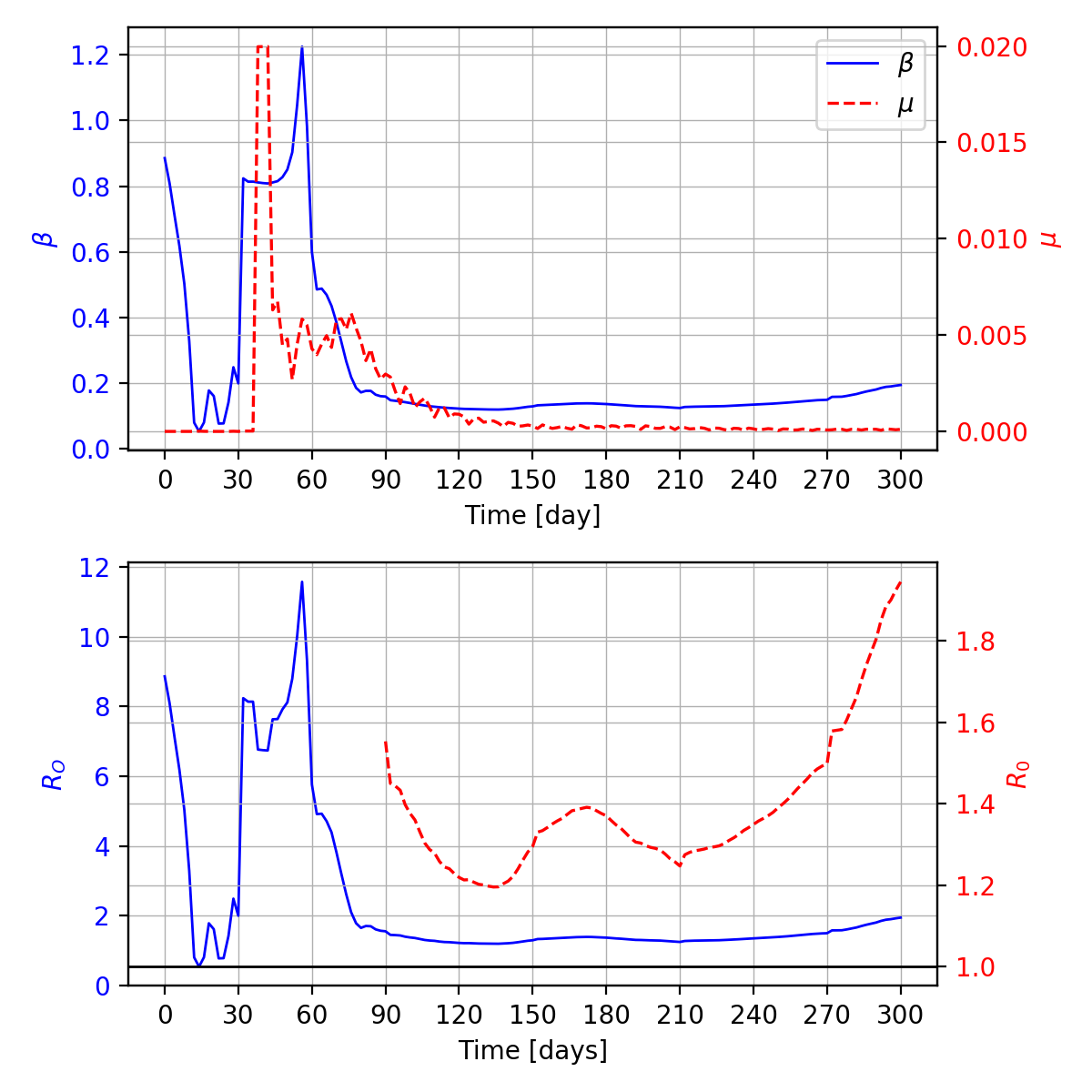
(b)

Figure 1. (a) Reported and fitted cumulative infection and death cases in the US (b) Estimated SEIR parameters and the basic reproduction number. $\beta$ ($\mu$) corresponds to the left (right) vertical axis, $\epsilon=0.2$ and $\gamma=0.1$ are almost constant. The dashed line in $R_{0}$ is a zoomed-in version on the tail of the solid line.

4. Experiments

We now present experimental results to demonstrate the good performance of our algorithms. In all the experiments, the normalization factors $\lambda_{1}$, $\lambda_{2}$ in (2.3) are chosen such that the loss with respect to the infection cases is at the same scale as the loss with respect to the death cases. According to the Centers for Disease Control and Prevention (CDC) in the US, the median incubation period is 4-5 days from exposure to symptoms onset, persons with mild to moderate COVID-19 remain infectious no longer than 10 days after symptom onset, therefore, we set

$$\Theta=\{\theta\>|\>0\leq\beta\leq 5,\;0.2\leq\epsilon\leq 0.25,\;0.1\leq\gamma\leq 0.2,\;0\leq\mu\leq 0.01\}.$$

For the step size, considering that $\beta$, $\epsilon$ and $\gamma$ are almost at the same scale, which is $100$ times greater than $\mu$, and the permissible range of $\beta$ is much large than $\epsilon$ and $\gamma$, we set $\tau_{\epsilon}=\tau_{\gamma}=\tau$, $\tau_{\beta}=100\tau$ and $\tau_{\mu}=\tau/100$.

4.1. Covid-19 epidemic in the US

As of today [November 17, 2020], it has been about $300$ days since the first infection case of COVID-19 was reported in the US. We thus consider the time period $[0,300]$ and sample the data $[I_{c},D_{c}]$ at $t_{i}=2i$ for $0<i\leq 150$. To apply Algorithm 2 we take $\{t_{n_{j}}\}_{j=0}^{s+1}$ as $\{$0, 30, 60, 90, 150, 210, 270, 300$\}$.

Data fitting via optimal control with SEIR model. Figure 1 (a) shows that our data-driven optimal control algorithm learns the data very well. In Figure 1 (b), there is a noticeable peak over the second month, where the value of reproduction number $R_{0}$ is very large due to a dramatic increase in infection rate $\beta$. After that, $R_{0}$ goes down to a lower range, with a slight rise around the $6$-th month. Over the last two months we observed another increase in $R_{0}$. Overall, the value of $R_{0}$ stays above $1$ and the pattern of $R_{0}$ is consistent with the increasing trend of the confirmed cases. For a short time period, one may expect the transmission to continue the same way, then the learned model parameters could be used for prediction over a short coming period.

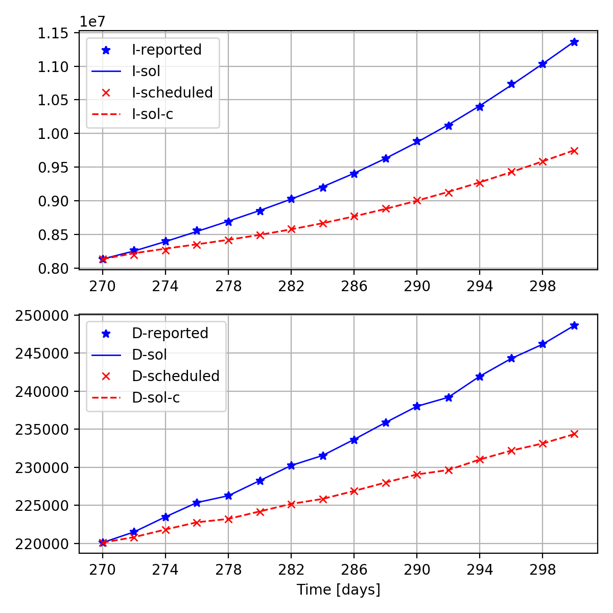
(a)

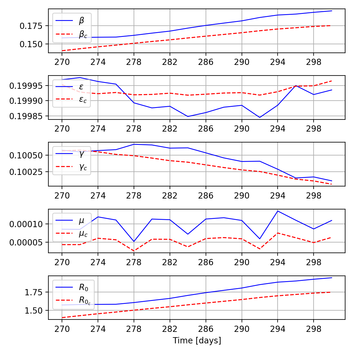
(b)

Figure 2. Scheduled control for the US in $270-300$ days by SEIR model

Scheduled control. From the above prediction result, we see that without interventions, the amount of confirmed and death cases will increase rapidly. We would like to see a slow down of the epidemic spreading as the outcome of various public health interventions. With the present approach, this can be formulated as a scheduled control. Specifically, with a desired level of infection and death cases at the final time $T$, we schedule a sequence of values at intermediate times, from which we apply our algorithm to learn the optimal parameters (control function) such that the state function reaches the desired value at $T$ along the scheduled path.

For instance, starting from the $270$-th day, with the goal of controlling the cumulative number of infection and death cases at $9,746,063$ and $234,390$ on the $300$-th day, respectively, we set a pair of values for each day in the $30$ days as shown in Figure 2 (a), then learn the parameters from the scheduled data. The results are presented in 2 (b). Figure 2 (a) shows that the goal can be achieved by setting the parameters as what have been learned.

To compare the situations with or without a scheduled control, we also present the reported data and corresponding training results in Figure 2. In fact, the scheduled intermediate values are obtained by assuming the daily increases were half of the reported daily increases. From Figure 2 (b), we see that the most significant difference occurs in $\beta$. This can be roughly interpreted as: if the contact rate $\beta$ could be reduced by $0.02$, the number of confirmed cases over the last $30$ days could have been reduced by $50\%$, though the corresponding $R_{0}$ is still greater than $1$. For virus propagation to eventually stop, $R_{0}$ needs to be less than $1$, for which $\beta$ must be less than $\gamma+\mu$.

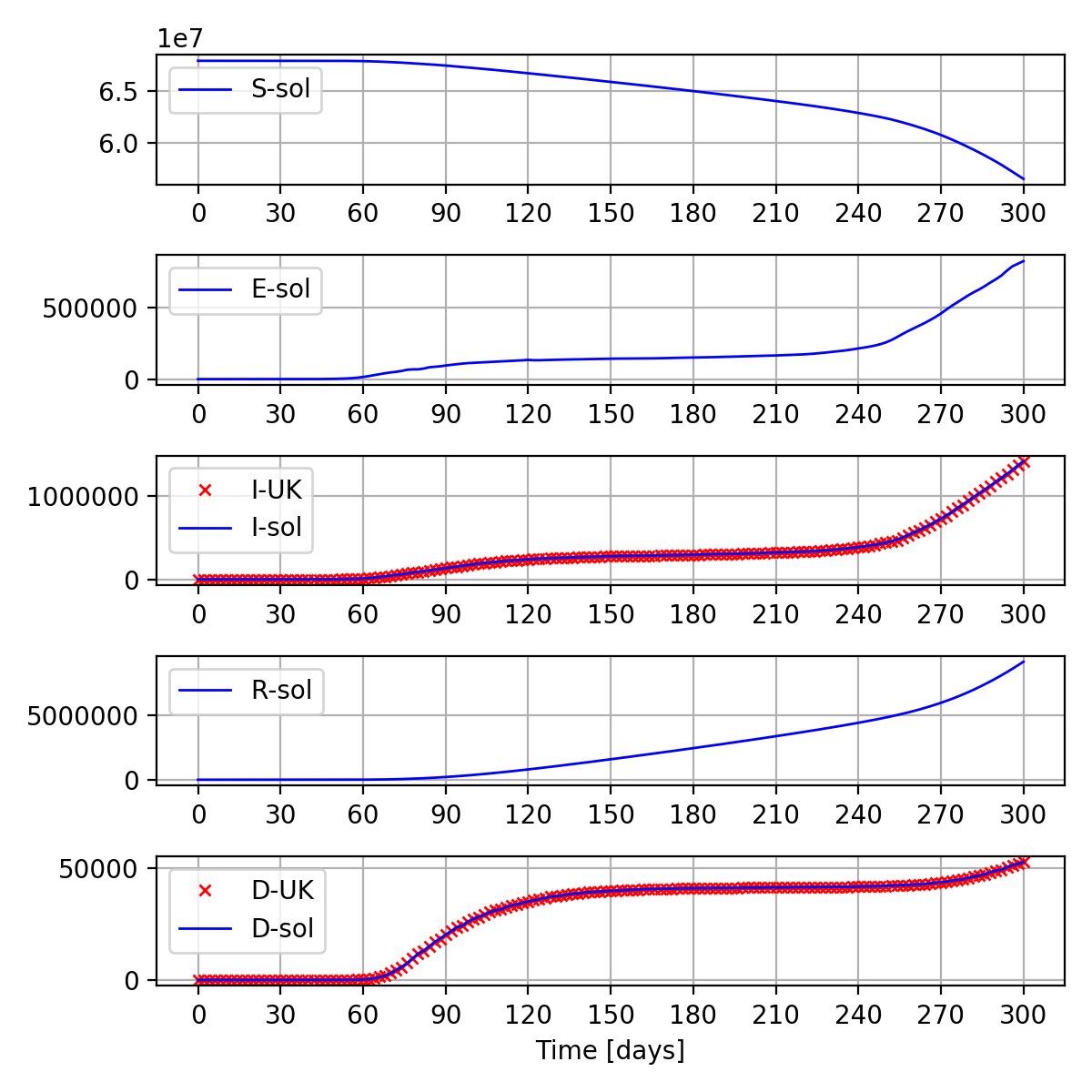
(a)

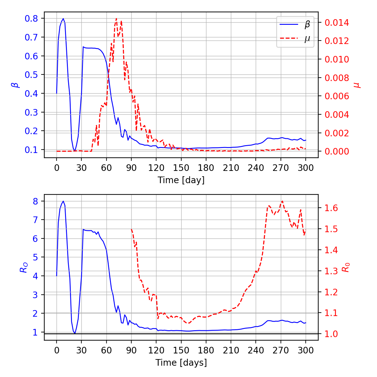
(b)

Figure 3. (a) Reported and fitted cumulative infection and death cases in the UK (b) Estimated SEIR parameters and the basic reproduction number. $\beta$ ($\mu$) corresponds to the left (right) vertical axis, $\epsilon=0.2$ and $\gamma=0.1$ are almost constant. The dashed line in $R_{0}$ is a zoomed-in version on the tail of the solid line.

4.2. Experimental results for other countries

The coronavirus pandemic continues to affect every region of the world, but some countries are experiencing higher rates of infection, while others appear to have mostly controlled the virus. In order to see the virus dynamics in other regions, we also provide results for some other selected countries such as the UK, France and China. For the UK, $\{t_{n_{j}}\}_{j=0}^{s+1}$ are taken as $\{$0, 30, 90, 120, 150, 180, 210, 240, 300$\}$. For France, $\{t_{n_{j}}\}_{j=0}^{s+1}$ are taken as $\{$0, 30, 60, 90, 180, 300$\}$. For China, $\{t_{n_{j}}\}_{j=0}^{s+1}$ are taken as $\{$0, 30, 60, 90, 120, 150, 180, 210, 240, 270, 300$\}$.

From Figure 3 and 4, we see that the confirmed cases in UK and France display similar patterns. Figure 5 shows that China was hit hard early on, but the number of new cases has largely been under control for months.

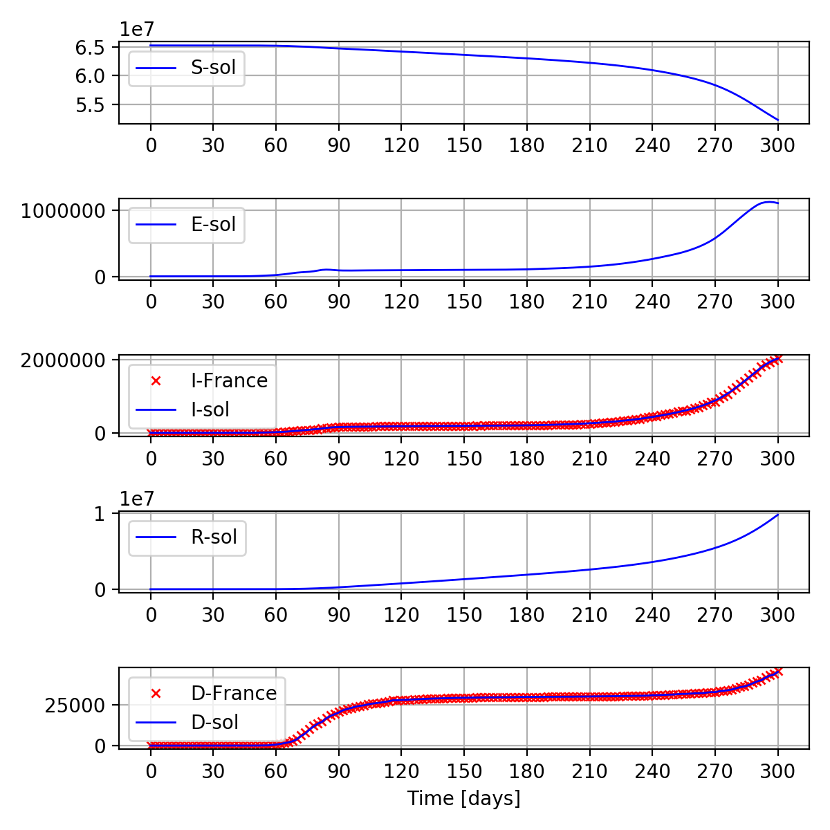
(a)

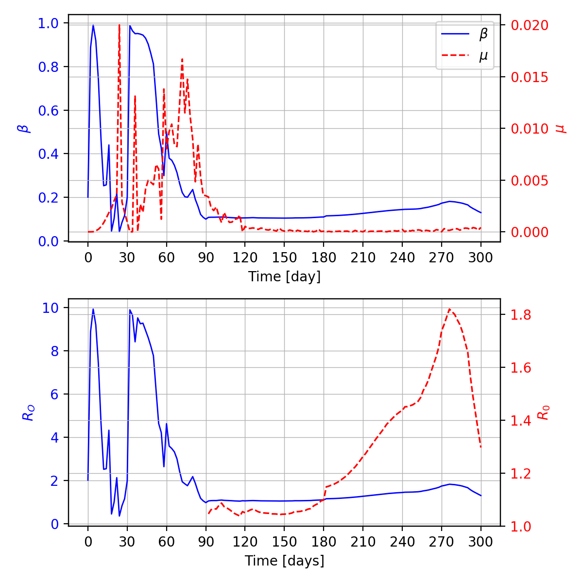
(b)

Figure 4. (a) Reported and fitted cumulative infection and death cases in France (b) Estimated SEIR parameters and the basic reproduction number. $\beta$ ($\mu$) corresponds to the left (right) vertical axis, $\epsilon=0.2$ and $\gamma=0.1$ are almost constant. The dashed line in $R_{0}$ is a zoomed-in version on the tail of the solid line.

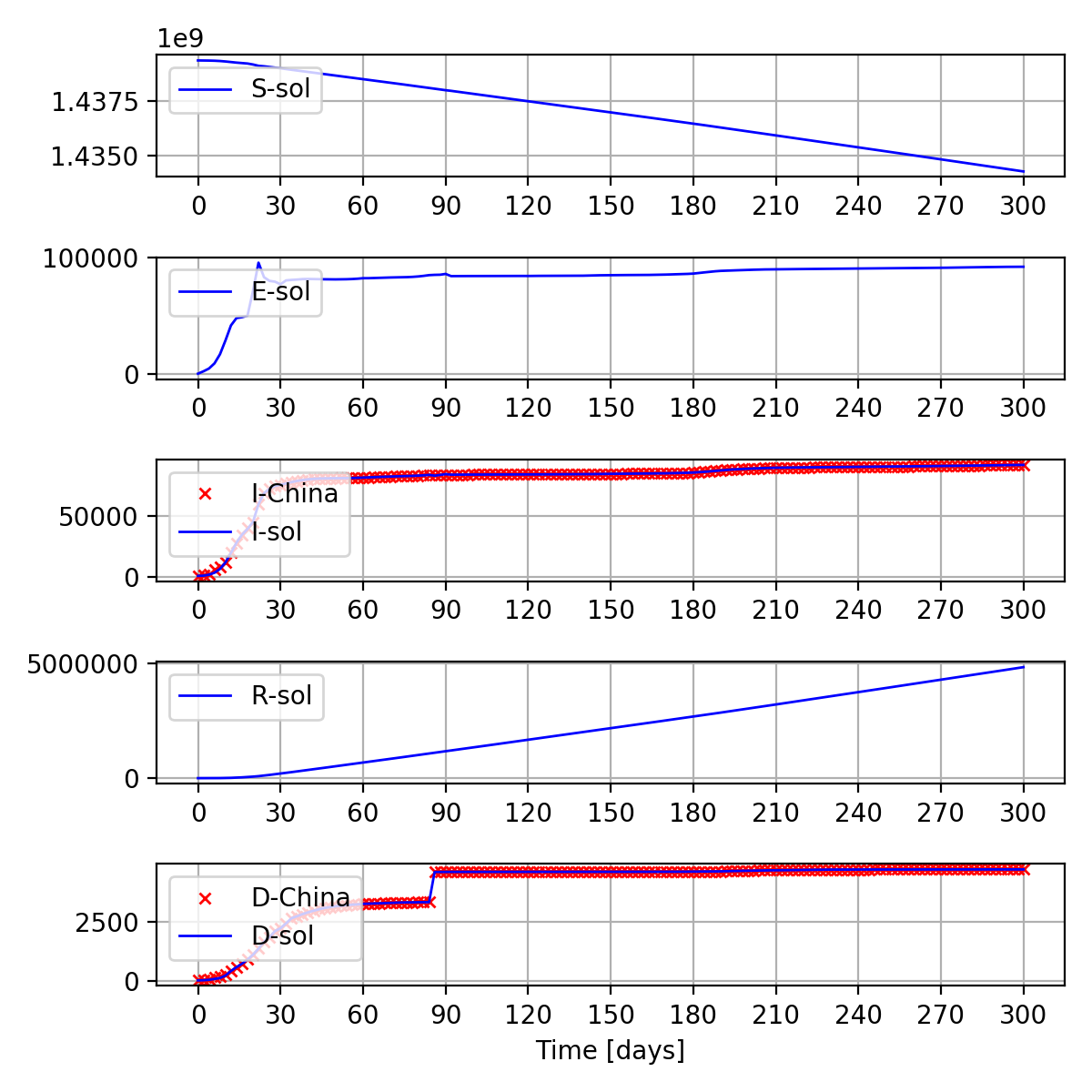
(a)

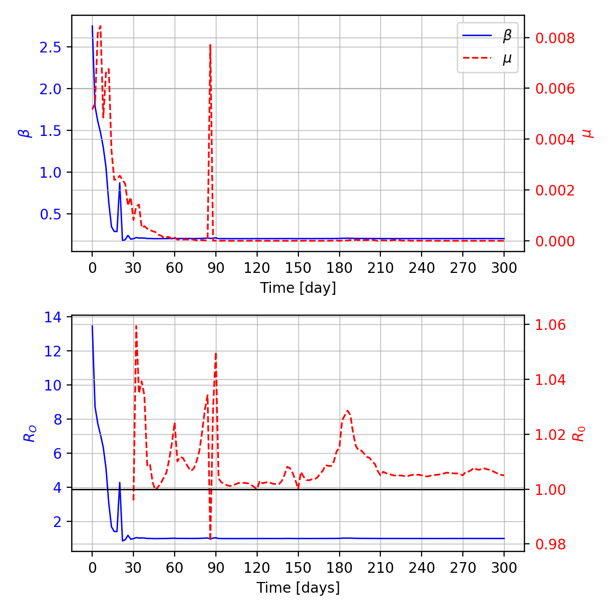
(b)

Figure 5. (a) Reported and fitted cumulative infection and death cases in China (b) Estimated SEIR parameters and the basic reproduction number. $\beta$ ($\mu$) corresponds to the left (right) vertical axis, $\epsilon=0.2$ and $\gamma=0.2$ are almost constant. The dashed line in $R_{0}$ is a zoomed-in version on the tail of the solid line.

5. Discussion

In this paper, we introduced a data-driven optimal control model for learning the time-varying parameters of the SEIR model, which reveals the virus spreading process among several population groups. Here the state variables represent the population status, such as $S,E,I,R,D$ while the control variables are rate parameters of transmission between population groups. The running cost is of discrete form fitting the reported data of infection and death cases at the observation times. The terminal cost can be used to quantify the desired level of the total infection and death cases at scheduled times. Numerical algorithms are derived to solve the proposed model efficiently. Experimental results show that our approach can effectively fit, predict and control the infected and deceased populations.

The data-driven modeling approach presented in this work is applicable to more advanced models such as with spatial movement effects, interaction of different class of populations, for which we need to formulate mean-field game type models over a spatial domain, see [36] for the mean-field game formulation of a epidemic control problem. On the computational side, our approach involves a non-convex optimization problem, which comes from the multiplicative terms of the SEIR model itself. In future work, we intend to extend our algorithm to more advanced models.

References

- [1] Vladimir V Aleksandrov, On the accumulation of perturbations in the linear systems with two coordinates, Vestnik MGU 3 (1968).
- [2] Linda J. S. Allen, An introduction to stochastic epidemic models, Mathematical epidemiology, vol. 1945, Springer, Berlin, 2008, pp. 81–130.
- [3] Cleo Anastassopoulou, Lucia Russo, Athanasios Tsakris, and Constantinos Siettos, Data-based analysis, modelling and forecasting of the COVID-19 outbreak, PLOS ONE 15 (2020), 1–21.
- [4] Roy M. Anderson and Robert M. May, Population biology of infectious diseases: Part I, Nature 280 (1979), 361–367.
- [5] Sercan Arik, Chun-Liang Li, Jinsung Yoon, Raj Sinha, Arkady Epshteyn, Long T. Le, Vik Menon, Shashank Singh, Leyou Zhang, Martin Nikoltchev, Yash Kumar Sonthalia, Hootan Nakhost, Elli Kanal, and Tomas Pfister, Interpretable sequence learning for covid-19 forecasting, ArXiv abs/2008.00646 (2020).
- [6] Chris T. Bauch and David J. D. Earn, Vaccination and the theory of games, Proc. Natl. Acad. Sci. USA 101 (2004), no. 36, 13391–13394.
- [7] H. Behncke, Optimal control of deterministic epidemics, Optimal control applications and methods 21(6) (2000), 269–285.
- [8] Henri Berestycki, Jean-Michel Roquejoffre, and Luca Rossi, Propagation of epidemics along lines with fast diffusion, ArXiv abs/2005.01859 (2020).
- [9] Andrea Bertozzi, Elisa Franco, George Mohler, Martin Short, and Daniel Sledge, The challenges of modeling and forecasting the spread of COVID-19, Proceedings of the National Academy of Sciences 117 (2020), 16732–16738.
- [10] Fred Brauer and Carlos Castillo-Chávez, Mathematical models in population biology and epidemiology, Texts in Applied Mathematics, vol. 40, Springer-Verlag, New York, 2001. MR 1822695
- [11] Alberto Bressan and Benedetto Piccoli, Introduction to the mathematical theory of control, AIMS Series on Applied Mathematics, vol. 2, American Institute of Mathematical Sciences (AIMS), Springfield, MO, 2007. MR 2347697
- [12] V. Capasso, Reaction-diffusion models for the spread of a class of infectious diseases, Proceedings of the Second European Symposium on Mathematics in Industry (Oberwolfach, 1987), European Consort. Math. Indust., vol. 3, Teubner, Stuttgart, 1988, pp. 181–194. MR 1128118
- [13] F. Castiglione and B. Piccoli, Cancer immunotherapy, mathematical modeling and optimal control, Journal of Theoretical Biology 247(4) (2007), 723–732.
- [14] Sheryl L. Chang, Mahendra Piraveenan, Philippa Pattison, and Mikhail Prokopenko, Game theoretic modelling of infectious disease dynamics and intervention methods: a review, Journal of Biological Dynamics 14 (2020), no. 1, 57–89.
- [15] Ricky T. Q. Chen, Yulia Rubanova, Jesse Bettencourt, and David K Duvenaud, Neural ordinary differential equations, Conference on Neural Information Processing Systems (NIPS), 2018.
- [16] F. L. Chernous and A. A. Lyubushin, Method of successive approximations for solution of optimal control problems, Optimal Control Appl. Methods 3 (1982), no. 2, 101–114.
- [17] Miles Cranmer, Sam Greydanus, Stephan Hoyer, Peter Battaglia, David Spergel, and Shirley Ho, Lagrangian neural networks, ArXiv abs/2003.04630 (2020).
- [18] Odo Diekmann and J. A. P. Heesterbeek, Mathematical epidemiology of infectious diseases, Wiley Series in Mathematical and Computational Biology, John Wiley and Sons, Ltd., Chichester, 2000, Model building, analysis and interpretation. MR 1882991
- [19] Weinan E, A proposal on machine learning via dynamical systems, Math. Sci. 5(1) (2017), 1–11.
- [20] Giulia Giordano, Franco Blanchini, Raffaele Bruno, Patrizio Colaneri, Alessandro Filippo, Angela Matteo, and Marta Colaneri, Modelling the COVID-19 epidemic and implementation of population-wide interventions in italy, Nature Medicine 26 (2020), 1–6.
- [21] D. Greenhalgh, Hopf bifurcation in epidemic models with a latent period and nonpermanent immunity, Mathematical and Computer Modelling 25(2) (1997), 85–107.
- [22] D. Greenhalgh and R. Das, Modeling epidemics with variable contact rates, Theoretical Population Biology 47(2) (1995), 129–179.
- [23] Sam Greydanus, Misko Dzamba, and Jason Yosinski, Hamiltonian neural networks, CoRR abs/1906.01563 (2019).
- [24] Magnus R. Hestenes, Calculus of variations and optimal control theory, John Wiley & Sons, Inc., New York-London-Sydney, 1966. MR 0203540
- [25] Herbert W. Hethcote, The mathematics of infectious diseases, SIAM Review 42(4) (2000), 599–653.
- [26] Yuzo Hosono and Bilal Ilyas, Traveling waves for a simple diffusive epidemic model, Math. Models Methods Appl. Sci. 5 (1995), no. 7, 935–966. MR 1359215
- [27] Elizabeth Hunter, Brian Mac Namee, and John Kelleher, An open-data-driven agent-based model to simulate infectious disease outbreaks, PLOS ONE 13 (2018), no. 12, 1–35.
- [28] Junyoung Jang, Hee Dae Kwon, and Jeehyun Lee, Optimal control problem of an SIR reaction–diffusion model with inequality constraints, Mathematics and Computers in Simulation 171 (2020), 136–151.
- [29] Hyeontae Jo, Hwijae Son, Hyung Ju Hwang, and Se Young Jung, Analysis of COVID-19 spread in South Korea using the SIR model with time-dependent parameters and deep learning, medRxiv (2020).
- [30] Matt Keeling and Ken Eames, Networks and epidemic models, Journal of the Royal Society, Interface / the Royal Society 2 (2005), 295–307.
- [31] David G Kendall, Mathematical models of the spread of infection, Mathematics and computer science in biology and medicine 171 (1965), 213–225.
- [32] W. O. Kermack and A. G. McKendrick, A contribution to the mathematical theory of epidemics, Proceedings of the Royal Society of London Series A 115(772) (1927), 700–721.
- [33] Adam Kleczkowski and Bryan T. Grenfell, Mean-field-type equations for spread of epidemics: The ‘small world’ model, Physica A: Statistical Mechanics and its Applications 274 (1999), no. 1-2, 355–360.
- [34] Andrei Korobeinikov, Global properties of SIR and SEIR epidemic models with multiple parallel infectious stages, Bull. Math. Biol. 71 (2009), no. 1, 75–83. MR 2469618
- [35] I. A. Krylov and F. L. Černous’ ko, The method of successive approximations for solving optimal control problems, Ž. Vyčisl. Mat i Mat. Fiz. 2 (1962), 1132–1139. MR 149044
- [36] Wonjun Lee, Siting Liu, Hamidou Tembine, Wuchen Li, and Stanley Osher, Controlling propagation of epidemics via mean-field games, ArXiv abs/2006.01249 (2020).
- [37] Michael Y. Li, John R. Graef, Liancheng Wang, and János Karsai, Global dynamics of a SEIR model with varying total population size, Mathematical Biosciences 160(2) (1999), 191–213.
- [38] Michael Y. Li and James S. Muldowney, Global stability for the SEIR model in epidemiology, Mathematical Biosciences 125(2) (1995), 155–164.
- [39] Qianying Lin, Shi Zhao, Daozhou Gao, Yijun Lou, Shu Yang, Salihu Musa, Maggie Wang, Weiming Wang, Lin Yang, and Daihai He, A conceptual model for the outbreak of coronavirus disease 2019 (COVID-19) in Wuhan, China with individual reaction and governmental action, International Journal of Infectious Diseases 93 (2020), 211–216.
- [40] Hailiang Liu and Peter Markowich, Selection dynamics for deep neural networks, J. Differential Equations 269 (2020), no. 12, 11540–11574. MR 4152217
- [41] Weimin Liu, Herbert W. Hethcote, and Simon A. Levin, Dynamical behavior of epidemiological models with nonlinear incidence rates, Journal of Mathematical Biology 25 (1987), 359–380.
- [42] M. Lutter, C. Ritter, and J. Peters, Deep lagrangian networks: Using physics as model prior for deep learning, ArXiv abs/1907.04490 (2019).
- [43] Luca Magri and Nguyen Anh Khoa Doan, First-principles machine learning modelling of COVID-19, ArXiv abs/2004.09478 (2020).
- [44] Jaime Mena-Lorcat and Herbert W. Hethcote, Dynamic models of infectious diseases as regulators of population sizes, Journal of Mathematical Biology 30 (1992), 693–716.
- [45] Roni Parshani, Shai Carmi, and Shlomo Havlin, Epidemic threshold for the susceptible-infectious-susceptible model on random networks, Physical review letters 104 (2010), 258701.
- [46] L.S. Pontryagin, V.G Boltyanskii, R.V Gamkrelidze, and E.F. Mishchenko, The mathematical theory of optimal processes, CRC Press, 1962.
- [47] M. Raissi, P. Perdikaris, and G. E. Karniadakis, Physics-informed neural networks: a deep learning framework for solving forward and inverse problems involving nonlinear partial differential equations, J. Comput. Phys. 378 (2019), 686–707. MR 3881695
- [48] Timothy C. Reluga and Alison P. Galvani, A general approach for population games with application to vaccination, Math. Biosci. 230 (2011), no. 2, 67–78.
- [49] R. Tyrrell Rockafellar, Monotone operators and the proximal point algorithm, SIAM Journal on Control and Optimization 14(5) (1976), 877–898.
- [50] Werner H. Schmidt, Numerical methods for optimal control problems with ODE or integral equations, Large-scale scientific computing, Lecture Notes in Comput. Sci., vol. 3743, Springer, Berlin, 2006, pp. 255–262. MR 2248608
- [51] Ruoyan Sun, Global stability of the endemic equilibrium of multigroup SIR models with nonlinear incidence, Comput. Math. Appl. 60 (2010), no. 8, 2286–2291. MR 2725319
- [52] Horst R. Thieme, Epidemic and demographic interaction in the spread of potentially fatal diseases in growing populations, Mathematical Biosciences 111(1) (1992), 99–130.
- [53] M.K. Makc Tiberiu Harko, Francisco S.N. Lobo, Exact analytical solutions of the susceptible-infected-recovered (SIR) epidemic model and of the SIR model with equal death and birth rates, Applied Mathematics and Computation 236(1) (2014), 184–194.
- [54] P. van den Driessche and James Watmough, Reproduction numbers and sub-threshold endemic equilibria for compartmental models of disease transmission, Math. Biosci. 180 (2002), 29–48, John A. Jacquez memorial volume.
- [55] Duncan J. Watts, Small worlds, Princeton Studies in Complexity, Princeton University Press, Princeton, NJ, 1999, The dynamics of networks between order and randomness.
- [56] S. Hoya White, A. Martín del Rey, and G. Rodríguez Sánchez, Modeling epidemics using cellular automata, Appl. Math. Comput. 186 (2007), no. 1, 193–202. MR 2316504