Bifurcation Analysis of the Eigenstructure of the Discrete Single-curl Operator in Three-dimensional Maxwell’s Equations with Pasteur Media

Abstract

This paper focuses on studying the bifurcation analysis of the eigenstructure of the $\gamma$-parameterized generalized eigenvalue problem ($\gamma$-GEP) arising in three-dimensional (3D) source-free Maxwell’s equations with Pasteur media, where $\gamma$ is the magnetoelectric chirality parameter. For the weakly coupled case, namely, $\gamma<\gamma_{*}\equiv$ critical value, the $\gamma$-GEP is positive definite, which has been well-studied by Chern et. al, 2015. For the strongly coupled case, namely, $\gamma>\gamma_{*}$, the $\gamma$-GEP is no longer positive definite, introducing a totally different and complicated structure. For the critical strongly coupled case, numerical computations for electromagnetic fields have been presented by Huang et. al, 2018. In this paper, we build several theoretical results on the eigenstructure behavior of the $\gamma$-GEPs. We prove that the $\gamma$-GEP is regular for any $\gamma>0$, and the $\gamma$-GEP has $2\times 2$ Jordan blocks of infinite eigenvalues at the critical value $\gamma_{*}$. Then, we show that the $2\times 2$ Jordan block will split into a complex conjugate eigenvalue pair that rapidly goes down and up and then collides at some real point near the origin. Next, it will bifurcate into two real eigenvalues, with one moving toward the left and the other to the right along the real axis as $\gamma$ increases. A newly formed state whose energy is smaller than the ground state can be created as $\gamma$ is larger than the critical value. This stunning feature of the physical phenomenon would be very helpful in practical applications. Therefore, the purpose of this paper is to clarify the corresponding theoretical eigenstructure of 3D Maxwell’s equations with Pasteur media.

Key words. Bifurcation analysis, Eigenstructure, Maxwell’s equations, Pasteur media, Jordan block, Regular matrix pair.

AMS subject classifications. Primary: 15A18, 15A22; Secondary 65F15.

1 Introduction

The eigenstructure of the discrete single-curl operator $\nabla\times$ is fundamental and vital for efficient numerical simulations of complex materials. Here, complex materials, or physically, complex media, imply coupling effects between electric and magnetic fields. Bianisotropic material is an important class of complex media (see, e.g., [12, Section 5.3]), of which the coupling effects between electric and magnetic fields can be described by the Tellegen representation of the constitutive relations

$$\boldsymbol{B}=\boldsymbol{\mu}\boldsymbol{H}+\boldsymbol{\zeta}\boldsymbol{E},\qquad\boldsymbol{D}=\boldsymbol{\varepsilon}\boldsymbol{E}+\boldsymbol{\xi}\boldsymbol{H},$$

where $\boldsymbol{E},\boldsymbol{H},\boldsymbol{D},\boldsymbol{B}$ are the electric, the magnetic fields, the dielectric displacement, and the magnetic induction at the position $\boldsymbol{x}$, respectively, $\boldsymbol{\mu}$ is the permeability, $\boldsymbol{\varepsilon}$ is the permittivity, and $\boldsymbol{\zeta},\boldsymbol{\xi}$ are magnetoelectric parameters. Usually, $\boldsymbol{\mu},\boldsymbol{\varepsilon},\boldsymbol{\zeta},\boldsymbol{\xi}$ are dyadics (a.k.a. second-order tensors) of dimension three. In particular, a bianisotropic medium is also called a biisotropic medium, if $\boldsymbol{\mu},\boldsymbol{\varepsilon},\boldsymbol{\zeta},\boldsymbol{\xi}$ are scalar dyadics, or equivalently,

$$\boldsymbol{\mu}=\mu\boldsymbol{I},\quad\boldsymbol{\varepsilon}=\varepsilon\boldsymbol{I},\quad\boldsymbol{\zeta}=\zeta\boldsymbol{I},\quad\boldsymbol{\xi}=\xi\boldsymbol{I},$$

where $\boldsymbol{I}$ represents the identity dyadics. Specifically, a Pasteur medium (a.k.a. the reciprocal chiral medium) is a type of biisotropic media, where

$$\xi=\iota\gamma,\qquad\zeta=-\iota\gamma,\qquad\gamma\geq 0.$$ (1.1)

Mathematically, the propagation of electromagnetic waves in bianisotropic media is modeled by the three-dimensional (3D) frequency domain source-free Maxwell’s equations with the constitutive relations

$$\nabla\times\boldsymbol{E}=\hphantom{-}\iota\omega\boldsymbol{B},\qquad \nabla\cdot\boldsymbol{B}=0,$$

$$\nabla\times\boldsymbol{H}=-\iota\omega\boldsymbol{D},\qquad \nabla\cdot\boldsymbol{D}=0,$$

or equivalently,

$$\begin{bmatrix}\nabla\times&0\\ 0&\nabla\times\\ \end{bmatrix}\begin{bmatrix}\boldsymbol{E}\\ \boldsymbol{H}\\ \end{bmatrix}=\iota\omega\begin{bmatrix}\boldsymbol{\zeta}&\boldsymbol{\mu}\\ -\boldsymbol{\varepsilon}&-\boldsymbol{\xi}\\ \end{bmatrix}\begin{bmatrix}\boldsymbol{E}\\ \boldsymbol{H}\\ \end{bmatrix},\qquad\begin{bmatrix}\nabla\cdot{}&0\\ 0&\nabla\cdot{}\\ \end{bmatrix}\begin{bmatrix}\boldsymbol{D}\\ \boldsymbol{B}\\ \end{bmatrix}=0,$$

where $\omega$ is the frequency. The Bloch theorem, from the theorem named after F. Bloch (see, e.g., [10, p. 167]), implies that the solutions of the Schrödinger equation for a periodic potential must be of a quasi-periodic form, stating that

The eigenfunctions of the wave equation for a periodic potential are the product of a plane wave $\exp(\iota 2\pi\boldsymbol{k}\cdot\boldsymbol{x})$ times a function $u_{\boldsymbol{k}}(\boldsymbol{x})$ with the periodicity of the crystal lattice.

Based on the Bloch theorem, the Bloch eigenvectors $\boldsymbol{E}$ and $\boldsymbol{H}$ on any crystal lattice, satisfying the quasi-periodic conditions

$$\boldsymbol{E}(\boldsymbol{x}+\boldsymbol{a}_{\ell})=\boldsymbol{E}(\boldsymbol{x})\exp(\iota 2\pi\boldsymbol{k}\cdot\boldsymbol{a}_{\ell}),\qquad\boldsymbol{H}(\boldsymbol{x}+\boldsymbol{a}_{\ell})=\boldsymbol{H}(\boldsymbol{x})\exp(\iota 2\pi\boldsymbol{k}\cdot\boldsymbol{a}_{\ell})$$

are of interest, where $2\pi\boldsymbol{k}$ is the Bloch wave vector in the first Brillouin zone $\operatorname{\mathcal{B}}$, and $\boldsymbol{a}_{\ell},\ell=1,2,3$ are the lattice translation vectors (see, e.g., [9, p. 34]).

Using Yee’s scheme [13], a finite difference discretization that satisfies the source-free conditions and the quasi-periodicity conditions naturally, the discretized Maxwell’s equations are

$$\begin{bmatrix}C&0\\ 0&C^{\operatorname{H}}\\ \end{bmatrix}\begin{bmatrix}\boldsymbol{e}\\ \boldsymbol{h}\\ \end{bmatrix}=\iota\omega\begin{bmatrix}\zeta_{d}&\mu_{d}\\ -\varepsilon_{d}&-\xi_{d}\\ \end{bmatrix}\begin{bmatrix}\boldsymbol{e}\\ \boldsymbol{h}\\ \end{bmatrix},$$ (1.2)

where $\mu_{d}$, $\varepsilon_{d}$, $\xi_{d}$ and $\zeta_{d}$ are diagonal matrices, and $C$ is special structured, facilitating the introduction of the fast Fourier transform (FFT) to accelerate numerical simulations [3, 6, 8] (see 2.1-2.4 below, for details).

For the Pasteur media, the matrix pair in 1.2 is positive definite when the parameter $\gamma$ in 1.1 is small, but it becomes an indefinite pair as $\gamma$ becomes larger (see below). The weakly coupled case, namely, the case in which the matrix pair is positive definite, has been analyzed by Chern et al. [3] in 2015. For the strongly coupled case, the matrix pair is no longer a positive-definite matrix pair, introducing a totally different and complicated structure. For the critical strongly coupled case, numerical computations for the electromagnetic fields $\boldsymbol{E}$ and $\boldsymbol{H}$ have been studied by Huang et. al. [7], but lack of theory makes it difficult to guarantee that the numerical results are valid and reliable.

In this paper, we build several theoretical results on the eigenstructure behavior of the discrete single-curl operator in 3D Maxwell’s equations for Pasteur media:

1. The matrix pair in 1.2 is always regular regardless of how large $\gamma$ is;

2. The matrix pair 1.2 has $2\times 2$ Jordan blocks of the infinite eigenvalues at the critical value $\gamma=\gamma_{*}$. Then, the $2\times 2$ Jordan block will split into a pair of complex conjugate eigenvalues that move rapidly down and up and collide at some real point near the origin to form an associated $2\times 2$ Jordan block of a real eigenvalue;

3. This $2\times 2$ Jordan block will bifurcate into two real eigenvalues such that one moves toward the left and the other to the right along the real axis;

4. A newly formed state whose energy is smaller than the ground state can be created as $\gamma$ is larger than the critical value $\gamma_{*}$.

The feature exhibited by the physical phenomenon derived from the above three points (b)-(d) is an astonishing finding. This discovery would be very useful in practical applications. However, the corresponding theoretical eigenstructure behavior should first be clarified.

Notation. $\iota=\sqrt{-1}$ is the imaginary unit; $\mathrm{e}=\exp(1)$ is Euler’s number. For any $n\in\mathbb{N}$, $\eta_{n}=\mathrm{e}^{\frac{2\pi\iota}{n}}$ is an $n$th root of unity. For any index set $\mathcal{I}$, $I^{\mathcal{I}}$ denotes the diagonal matrix whose $i$th diagonal entry is $1$ for all $i\in\mathcal{I}$ and $0$ otherwise; $I^{\mathcal{I}}_{\sigma}$ denotes the matrix consisting of all nonzero columns of $I^{\mathcal{I}}$; and $|\mathcal{I}|$ denotes the number of its elements. $I_{n}$ is the identity matrix of size $n$; in particular, $I_{0}$ is an empty matrix; $e_{i}$ is the $i$th column of $I_{n}$. For a matrix $X$, $X^{\operatorname{T}}$ and $X^{\operatorname{H}}$ are its transpose and conjugate transpose, respectively; $\operatorname{\mathcal{N}}(X)=\{v:Xv=0\}$ is the kernel of $X$. For matrices $X,Y$, $X\otimes Y$ is their Kronecker product; $X\succeq Y$ means that $X-Y$ is positive semidefinite, similarly for “$\succ$”, “$\preceq$”, and “$\prec$”. For $m\in\mathbb{N}$, $\alpha\in\mathbb{C}$ and $X\in\mathbb{C}^{n\times n}$, write

$$V_{m\times n}(\alpha):=\begin{bmatrix}1&1&\cdots&1\\ \alpha&\alpha^{2}&\cdots&\alpha^{n}\\ \vdots&\vdots&&\vdots\\ \alpha^{m-1}&\alpha^{2(m-1)}&\cdots&\alpha^{n(m-1)}\\ \end{bmatrix},\quad K_{m}(X):=\begin{bmatrix}&I_{n}&&\\ &&\ddots&\\ &&&I_{n}\\ X&&&\\ \end{bmatrix}_{mn\times mn}.$$

In particular, write $V_{m}(\alpha)=V_{m\times 1}(\alpha)$, $D_{m}(\alpha)=\alpha\operatorname{diag}(V_{m}(\alpha))$.

2 Preliminaries

2.1 Discretization

It is well known from crystallography that crystal structures can be classified into 14 Bravais lattices [1, 2]. Because of various lattices, the discretized single-curl operators $C$ and $C^{\operatorname{H}}$ in 1.2 on the electric and magnetic fields, respectively, may have different forms. In the discretization process, $\operatorname{\mathcal{D}}_{i}$ and $\operatorname{\mathcal{D}}_{o}$ denote the sets including the indices of all vertices inside and outside, respectively, the medium (usually the domain would be of vacuum or air but could be of another medium). Then, $\operatorname{\mathcal{D}}=\operatorname{\mathcal{D}}_{i}\cup\operatorname{\mathcal{D}}_{o}$ is the discretization grid. Moreover, $n_{1},n_{2},n_{3}$ denote the numbers of grid vertices in the $x,y,z$ directions, respectively, and $\delta_{1},\delta_{2},\delta_{3}$ for the associated mesh lengths. Write $n=n_{1}n_{2}n_{3}$.

The discretized Maxwell’s equations are 1.2, in which $\zeta_{d}$, $\mu_{d}$, $\varepsilon_{d}$, $\xi_{d}$ are decided by the shape of the medium, and $C$ is given by Yee’s scheme. For the former, $\zeta_{d}$, $\mu_{d}$, $\varepsilon_{d}$, $\xi_{d}$ may not have the same value in three directions of some boundary points. However, for convenience of notation, in this paper, we consider the case that

$$\mu_{d} =\mu_{io}I_{3}\otimes I,\qquad\varepsilon_{d}=I_{3}\otimes[\varepsilon_{o}I^{(o)}+\varepsilon_{i}I^{(i)}],$$ (2.1a)

$$\zeta_{d} =-\iota\gamma I_{3}\otimes I^{(i)},\qquad\xi_{d}=\iota\gamma I_{3}\otimes I^{(i)},$$ (2.1b)

where $\gamma$ is the chirality, $\varepsilon_{i},\varepsilon_{o}$ are the permittivities inside and outside the medium, respectively, and $\mu_{io}\equiv 1$ is the permeability. For simplicity, here we denote $I^{(i)}\equiv I^{\operatorname{\mathcal{D}}_{i}}$ and $I^{(o)}\equiv I^{\operatorname{\mathcal{D}}_{o}}$.

For the latter, we refer the readers to [8] in order to peruse the details of the whole discretization process. We provide some basic but important results to ensure this paper is self-contained. According to the type of the lattice, one of the 14 Bravais lattices, which represent all kinds of crystals, $C$, the discretized single-curl operator on the electric field by Yee’s scheme, may have different forms which can be uniformly written as

$$C=\begin{bmatrix}0&-C_{3}&C_{2}\\ C_{3}&0&-C_{1}\\ -C_{2}&C_{1}&0\end{bmatrix},$$ (2.2)

where

$$C_{1} =\delta_{1}^{-1}[-I_{n}+I_{n_{3}}\otimes I_{n_{2}}\otimes K_{n_{1}}(\mathrm{e}^{\iota 2\pi\boldsymbol{k}\cdot\boldsymbol{a}_{1}})],$$ (2.3a)

$$C_{2} =\delta_{2}^{-1}[-I_{n}+I_{n_{3}}\otimes K_{n_{2}}(\mathrm{e}^{\iota 2\pi\boldsymbol{k}\cdot\boldsymbol{a}_{2}}J_{1})],$$ (2.3b)

$$C_{3} =\delta_{3}^{-1}[-I_{n}+K_{n_{3}}(\mathrm{e}^{\iota 2\pi\boldsymbol{k}\cdot\boldsymbol{a}_{3}}J_{2})],$$ (2.3c)

with $J_{1}=J_{1,1}$ and

$$J_{2} =\mathrm{e}^{\iota 2\pi\boldsymbol{k}\cdot\rho_{2}\boldsymbol{a}_{2}}\begin{bmatrix}&\mathrm{e}^{-\iota 2\pi\boldsymbol{k}\cdot\boldsymbol{a}_{2}}I_{m_{2}}\otimes J_{1,3}\\ I_{n_{2}-m_{2}}\otimes J_{1,2}&\\ \end{bmatrix},$$ (2.4a)

$$J_{1,\ell} =\mathrm{e}^{\iota 2\pi\boldsymbol{k}\cdot\rho_{1,\ell}\boldsymbol{a}_{1}}\begin{bmatrix}&\mathrm{e}^{-\iota 2\pi\boldsymbol{k}\cdot\boldsymbol{a}_{1}}I_{m_{1,\ell}}\\ I_{n_{1}-m_{1,\ell}}&\\ \end{bmatrix},\qquad\ell=1,2,3.$$ (2.4b)

Here, $\rho_{2},\rho_{1,1}\in\{0,1\}$, $\rho_{1,2},\rho_{1,3}\in\{-1,0,1,2\}$ satisfying $\rho_{1,2}-\rho_{1,3}-\rho_{1,1}\in\{0,1\}$, and $m_{2}\in[0,n_{2}]\cap\mathbb{N}$, $m_{1,\ell}\in[0,n_{1}]\cap\mathbb{N}$ for $\ell=1,2,3$ satisfying $m_{1,2}-m_{1,3}-m_{1,1}\in\{0,n_{1}\}$. Write $m_{1}:=m_{1,1}$, $\rho_{1}:=\rho_{1,1}$, and $\widehat{\rho}_{1}:=\rho_{2}\rho_{1}+\rho_{2}\rho_{1,2}+(1-\rho_{2})\rho_{1,3}$.

$C_{1},C_{2},C_{3}$ are simultaneously diagonalizable by a unitary matrix, which is guaranteed by theorem 2.1.

Theorem 2.1 ([8]).

$C_{1},C_{2},C_{3}$ are simultaneously diagonalizable by the unitary matrix $T=[t_{\ell}]_{\ell=1,\dots,n}$ in the forms

$$\Lambda_{1}:=T^{\operatorname{H}}C_{1}T =\delta_{1}^{-1}[-I_{n}+\eta_{n_{1}}^{\boldsymbol{k}\cdot\widehat{\boldsymbol{a}}_{1}}I_{n_{3}}\otimes I_{n_{2}}\otimes D_{n_{1}}(\eta_{n_{1}})],$$ (2.5a)

$$\Lambda_{2}:=T^{\operatorname{H}}C_{2}T =\delta_{2}^{-1}[-I_{n}+\eta_{n_{2}}^{\boldsymbol{k}\cdot\widehat{\boldsymbol{a}}_{2}}I_{n_{3}}\otimes D_{n_{2}}(\eta_{n_{2}})\otimes D_{n_{1}}(\eta_{n_{1}n_{2}}^{-m_{1}})],$$ (2.5b)

$$\Lambda_{3}:=T^{\operatorname{H}}C_{3}T =\delta_{3}^{-1}[-I_{n}+\eta_{n_{3}}^{\boldsymbol{k}\cdot\widehat{\boldsymbol{a}}_{3}}D_{n_{3}}(\eta_{n_{3}})\otimes D_{n_{2}}(\eta_{n_{3}n_{2}}^{-m_{2}})\otimes D_{n_{1}}(\eta_{n_{1}n_{3}}^{-\widehat{m}_{1}}\eta_{n_{1}n_{2}n_{3}}^{m_{1}m_{2}})],$$ (2.5c)

where

$$\!\!t_{\langle i_{1},i_{2},i_{3}\rangle}\!=\!\tfrac{1}{\sqrt{n}}V_{n_{3}}(\eta_{n_{3}}^{\boldsymbol{k}\cdot\widehat{\boldsymbol{a}}_{3}+i_{3}}\eta_{n_{2}n_{3}}^{-m_{2}i_{2}}\eta_{n_{1}n_{3}}^{-\widehat{m}_{1}i_{1}}\eta_{n_{1}n_{2}n_{3}}^{m_{1}m_{2}i_{1}})\otimes V_{n_{2}}(\eta_{n_{2}}^{\boldsymbol{k}\cdot\widehat{\boldsymbol{a}}_{2}+i_{2}}\eta_{n_{1}n_{2}}^{-m_{1}i_{1}})\otimes V_{n_{1}}(\eta_{n_{1}}^{\boldsymbol{k}\cdot\widehat{\boldsymbol{a}}_{1}+i_{1}})$$ (2.6)

for $i_{1},i_{2},i_{3}\in\mathbb{Z}$, $\langle i_{1},i_{2},i_{3}\rangle$ is defined as

$$\langle i_{1},i_{2},i_{3}\rangle:=(i_{3}^{\prime}-1)n_{1}n_{2}+(i_{2}^{\prime}-1)n_{1}+i_{1}^{\prime},$$

where $i_{\ell}^{\prime}=i_{\ell}+t_{\ell}n_{\ell},1\leq i_{\ell}^{\prime}\leq n_{\ell},t_{\ell}\in\mathbb{Z},\ell=1,2,3$, and

$$\widehat{\boldsymbol{a}}_{1} =\boldsymbol{a}_{1},$$

$$\widehat{\boldsymbol{a}}_{2} =\boldsymbol{a}_{2}+(\rho_{1}-\frac{m_{1}}{n_{1}})\widehat{\boldsymbol{a}}_{1},$$

$$\widehat{\boldsymbol{a}}_{3} =\boldsymbol{a}_{3}+(\rho_{2}-\frac{m_{2}}{n_{2}})\widehat{\boldsymbol{a}}_{2}+[\widehat{\rho}_{1}-\frac{\widehat{m}_{1}}{n_{1}}-\rho_{2}(\rho_{1}-\frac{m_{1}}{n_{1}})]\widehat{\boldsymbol{a}}_{1},$$

$$\widehat{m}_{1} =\rho_{2}m_{1}+\rho_{2}m_{1,2}+(1-\rho_{2})m_{1,3}.$$

Note that

1. $\widehat{\boldsymbol{a}}_{1},\widehat{\boldsymbol{a}}_{2},\widehat{\boldsymbol{a}}_{3}$ is an orthogonal basis of $\boldsymbol{a}_{1},\boldsymbol{a}_{2},\boldsymbol{a}_{3}$, and $\|\widehat{\boldsymbol{a}}_{\ell}\|_{2}=l_{\ell}=n_{\ell}\delta_{\ell}$ for $\ell=1,2,3$.

2. $2\pi\boldsymbol{k}\in\mathcal{B}$ implies

   $$b_{l,\ell}\leq\boldsymbol{k}\cdot\boldsymbol{a}_{\ell}\leq b_{u,\ell},\qquad\ell=1,2,3,$$ (2.7)

   where $b_{u,\ell}-b_{l,\ell}\leq 1$, $b_{l,\ell}\in[-2/3,0],b_{u,\ell}\in[0,5/6]$.

As a result, the singular value decomposition of $C$ can be calculated along the way in [3], which is shown in theorem 2.2.

Theorem 2.2 ([3, 8]).

If $\boldsymbol{k}\neq 0$, then:

(a)

$\Lambda_{q}:=\Lambda_{1}^{\operatorname{H}}\Lambda_{1}+\Lambda_{2}^{\operatorname{H}}\Lambda_{2}+\Lambda_{3}^{\operatorname{H}}\Lambda_{3}\succ 0$;

(b)

$\Lambda_{p}:=\left(\begin{bmatrix}0&-\tau_{3}&\tau_{2}\\ \tau_{3}&0&-\tau_{1}\\ -\tau_{2}&\tau_{1}&0\\ \end{bmatrix}\otimes I_{n}\right)\begin{bmatrix}\Lambda_{1}^{\operatorname{H}}\\ \Lambda_{2}^{\operatorname{H}}\\ \Lambda_{3}^{\operatorname{H}}\\ \end{bmatrix}$ is of full column rank, provided $\tau_{1}\delta_{1}$, $\tau_{2}\delta_{2}$, $\tau_{3}\delta_{3}$ are distinct;

(c)

the singular value decomposition (SVD) of $C$ is

$$C =(I_{3}\otimes T)\begin{bmatrix}-\overline{\Pi_{2}}&\overline{\Pi_{1}}&\overline{\Pi_{0}}\end{bmatrix}\begin{bmatrix}\Lambda_{q}^{1/2}&&\\ &\Lambda_{q}^{1/2}&\\ &&0\\ \end{bmatrix}\begin{bmatrix}\Pi_{1}&\Pi_{2}&\Pi_{0}\end{bmatrix}^{\operatorname{H}}(I_{3}\otimes T^{\operatorname{H}})$$

$$\equiv\begin{bmatrix}P_{r}&P_{0}\end{bmatrix}\begin{bmatrix}\Sigma&0\\ 0&0\end{bmatrix}\begin{bmatrix}Q_{r}&Q_{0}\end{bmatrix}^{\operatorname{H}}=P_{r}\Sigma Q_{r}^{\operatorname{H}},$$ (2.8)

where

$$\Pi_{0}=\begin{bmatrix}\Lambda_{1}\\ \Lambda_{2}\\ \Lambda_{3}\\ \end{bmatrix}\!\Lambda_{q}^{-\frac{1}{2}},\Pi_{2}=\Lambda_{p}(\Lambda_{p}^{\operatorname{H}}\Lambda_{p})^{-\frac{1}{2}},\overline{\Pi_{1}}=\begin{bmatrix}0&-\Lambda_{3}&\Lambda_{2}\\ \Lambda_{3}&0&-\Lambda_{1}\\ -\Lambda_{2}&\Lambda_{1}&0\\ \end{bmatrix}\!\Lambda_{p}(\Lambda_{p}^{\operatorname{H}}\Lambda_{p}\Lambda_{q})^{-\frac{1}{2}}.$$

It is not difficult to observe that there is only one nonzero off-diagonal entry in each column or row of $C_{1},C_{2},C_{3}$. Physically, the entry represents the relation between a mesh node with its surroundings in the mesh grid, or equivalently, the neighbor in the lattice. The index of such an entry in $C_{1},C_{2},C_{3}$ is that of the neighbor of the node along $\boldsymbol{a}_{1},\boldsymbol{a}_{2},\boldsymbol{a}_{3}$. For ease, these $6$ neighbors of a node are called its lattice neighbors. Define

$$\operatorname{\mathcal{L}}_{\ell}(i_{1},i_{2},i_{3}):=\{\langle i_{1}^{\prime},i_{2}^{\prime},i_{3}^{\prime}\rangle:\text{$C_{\ell}(i_{\ell},i_{\ell}^{\prime})\neq 0$ or $C_{\ell}(i_{\ell}^{\prime},i_{\ell})\neq 0$}\},\qquad\ell=1,2,3,$$

and $\operatorname{\mathcal{L}}(i_{1},i_{2},i_{3}):=\operatorname{\mathcal{L}}_{1}(i_{1},i_{2},i_{3})\cup\operatorname{\mathcal{L}}_{2}(i_{1},i_{2},i_{3})\cup\operatorname{\mathcal{L}}_{3}(i_{1},i_{2},i_{3})$. Clearly, $\operatorname{\mathcal{L}}(i_{1},i_{2},i_{3})$ is the set of the node $\langle i_{1},i_{2},i_{3}\rangle$ and its 6 lattice neighbors. Furthermore,

$$e_{\langle i_{1},i_{2},i_{3}\rangle}^{\operatorname{H}}C_{\ell}I^{\operatorname{\mathcal{D}}\setminus\operatorname{\mathcal{L}}(i_{1},i_{2},i_{3})}_{\sigma}=0,\qquad e_{\langle i_{1},i_{2},i_{3}\rangle}^{\operatorname{H}}C_{\ell}^{\operatorname{H}}I^{\operatorname{\mathcal{D}}\setminus\operatorname{\mathcal{L}}(i_{1},i_{2},i_{3})}_{\sigma}=0.$$ (2.9)

Moreover, we can define the boundary and interior of an index set $\mathcal{I}$:

$$\partial\mathcal{I}:=\{\langle i_{1},i_{2},i_{3}\rangle\in\mathcal{I}:\operatorname{\mathcal{L}}(i_{1},i_{2},i_{3})\setminus\mathcal{I}\neq\emptyset\},\quad\mathcal{I}^{\circ}:=\{\langle i_{1},i_{2},i_{3}\rangle\in\mathcal{I}:\operatorname{\mathcal{L}}(i_{1},i_{2},i_{3})\subset\mathcal{I}\}.$$

2.2 Equivalence of generalized/quadratic eigenvalue problems (GEP /QEP)

It is easily seen that the GEP 1.2 can be rewritten as

$$\iota\begin{bmatrix}I_{3n}&0\\ -\xi_{d}\mu_{d}^{-1}&-I_{3n}\end{bmatrix}\left(\begin{bmatrix}0&-\iota C\\ \iota C^{\operatorname{H}}&\iota\xi_{d}\mu_{d}^{-1}C-\iota C^{\operatorname{H}}\mu_{d}^{-1}\zeta_{d}\end{bmatrix}-\omega\begin{bmatrix}\mu_{d}&0\\ 0&\varepsilon_{d}-\xi_{d}\mu_{d}^{-1}\zeta_{d}\end{bmatrix}\right)\\ \cdot\begin{bmatrix}I_{3n}&\mu_{d}^{-1}\zeta_{d}\\ 0&I_{3n}\end{bmatrix}\begin{bmatrix}\boldsymbol{h}\\ \boldsymbol{e}\end{bmatrix}=0.$$

Together with the choices of $\mu_{d},\varepsilon_{d},\zeta_{d},\xi_{d}$, we can consider this matrix pair instead

$$\begin{multlined}\begin{bmatrix}0&-\iota C\\ \iota C^{\operatorname{H}}&-\gamma[(I_{3}\otimes I^{(i)})C+C^{\operatorname{H}}(I_{3}\otimes I^{(i)})]\end{bmatrix}-\omega\begin{bmatrix}I_{3}\otimes I_{n}&0\\ 0&I_{3}\otimes[\varepsilon_{o}I^{(o)}+(\varepsilon_{i}-\gamma^{2})I^{(i)}]\end{bmatrix}\\ :=A_{\gamma}-\omega B_{\gamma},\end{multlined}\begin{bmatrix}0&-\iota C\\ \iota C^{\operatorname{H}}&-\gamma[(I_{3}\otimes I^{(i)})C+C^{\operatorname{H}}(I_{3}\otimes I^{(i)})]\end{bmatrix}-\omega\begin{bmatrix}I_{3}\otimes I_{n}&0\\ 0&I_{3}\otimes[\varepsilon_{o}I^{(o)}+(\varepsilon_{i}-\gamma^{2})I^{(i)}]\end{bmatrix}\\ :=A_{\gamma}-\omega B_{\gamma},$$ (2.10)

also written as a matrix pair $(A_{\gamma},B_{\gamma})$, which is equivalent to 1.2 in the sense that

$$\begin{multlined}\text{ $(\omega,\begin{bmatrix}\boldsymbol{h}-\iota\gamma(I_{3}\otimes I^{(i)})\boldsymbol{e}\\ \boldsymbol{e}\\ \end{bmatrix})$ is an eigenpair of \lx@cref{creftype~refnum}{eq:equivGEP} }\\ \Leftrightarrow\text{ $(\omega,\begin{bmatrix}\boldsymbol{e}\\ \boldsymbol{h}\\ \end{bmatrix})$ is an eigenpair of \lx@cref{creftype~refnum}{eq:maxwell-eq:discrete}. }\end{multlined}\text{ $(\omega,\begin{bmatrix}\boldsymbol{h}-\iota\gamma(I_{3}\otimes I^{(i)})\boldsymbol{e}\\ \boldsymbol{e}\\ \end{bmatrix})$ is an eigenpair of \lx@cref{creftype~refnum}{eq:equivGEP} }\\ \Leftrightarrow\text{ $(\omega,\begin{bmatrix}\boldsymbol{e}\\ \boldsymbol{h}\\ \end{bmatrix})$ is an eigenpair of \lx@cref{creftype~refnum}{eq:maxwell-eq:discrete}. }$$

Moreover, if $(\omega,\begin{bmatrix}\boldsymbol{e}\\ \boldsymbol{h}\\ \end{bmatrix})$ is an eigenpair of 1.2 with $\omega\neq 0$, then $\boldsymbol{h}=\iota(\gamma I_{3}\otimes I^{(i)}-\omega^{-1}C)\boldsymbol{e}$. Note that $A_{\gamma},B_{\gamma}$ are Hermitian; $(A_{\gamma},B_{\gamma})$ is regular if $\gamma\neq\gamma_{*}\equiv\sqrt{\varepsilon_{i}}$; $B_{\gamma}\succ 0$ if $\gamma<\gamma_{*}$; $B_{\gamma}$ is indefinite if $\gamma>\gamma_{*}$. Thus, all eigenvalues of $(A_{\gamma},B_{\gamma})$ are real if $\gamma<\gamma_{*}$.

The matrix pair $(A_{\gamma},B_{\gamma})$ is also equivalent to a Hermitian quadratic matrix polynomial (a Hermitian QEP)

$$Q_{\gamma}(\omega):=C^{\operatorname{H}}C-\omega\gamma[(I_{3}\otimes I^{(i)})C+C^{\operatorname{H}}(I_{3}\otimes I^{(i)})]-\omega^{2}I_{3}\otimes[\varepsilon_{o}I^{(o)}+(\varepsilon_{i}-\gamma^{2})I^{(i)}],$$ (2.11)

in the sense that for $\boldsymbol{e}\neq 0$,

$$(\omega,\boldsymbol{e}) \Leftrightarrow (\omega,\begin{bmatrix}\boldsymbol{e}\\ \boldsymbol{h}\\ \end{bmatrix})$$ is an eigenpair of 2.11 is an eigenpair of 1.2.

Clearly, the eigenvalues of $Q_{\gamma}(\cdot)$ are real or appear in conjugate pairs if nonreal.

Suppose that $\omega$ is an eigenvalue of $Q_{\gamma}(\cdot)$ and $\boldsymbol{e}$ is its corresponding eigenvector. Then, $Q_{\gamma}(\omega)\boldsymbol{e}=0$ gives

$$\boldsymbol{e}^{\operatorname{H}}Q_{\gamma}(\omega)\boldsymbol{e}=c(\boldsymbol{e})-\omega\gamma b(\boldsymbol{e})-\omega^{2}[\varepsilon_{o}a_{o}(\boldsymbol{e})+(\varepsilon_{i}-\gamma^{2})a_{i}(\boldsymbol{e})]=0,$$ (2.12)

where

$$c(\boldsymbol{e}) :=\boldsymbol{e}^{\operatorname{H}}C^{\operatorname{H}}C\boldsymbol{e}\geq 0,$$

$$b(\boldsymbol{e}) :=\boldsymbol{e}^{\operatorname{H}}[(I_{3}\otimes I^{(i)})C+C^{\operatorname{H}}(I_{3}\otimes I^{(i)})]\boldsymbol{e}=2\Re[\boldsymbol{e}^{\operatorname{H}}(I_{3}\otimes I^{(i)})C\boldsymbol{e}]\in\mathbb{R},$$

$$a_{o}(\boldsymbol{e}) :=\boldsymbol{e}^{\operatorname{H}}[I_{3}\otimes I^{(o)}]\boldsymbol{e}\geq 0,$$

$$a_{i}(\boldsymbol{e}) :=\boldsymbol{e}^{\operatorname{H}}[I_{3}\otimes I^{(i)}]\boldsymbol{e}\geq 0.$$

Furthermore,

$$c(\boldsymbol{e})=0\Leftrightarrow C\boldsymbol{e}=0,\quad a_{o}(\boldsymbol{e})=0\Leftrightarrow(I_{3}\otimes I^{(o)})\boldsymbol{e}=0,\quad a_{i}(\boldsymbol{e})=0\Leftrightarrow(I_{3}\otimes I^{(i)})\boldsymbol{e}=0.$$ (2.13)

By 2.12, $\omega$ is one of the roots of the scalar function

$$\omega_{\pm}(\boldsymbol{e})=\frac{\gamma b(\boldsymbol{e})\pm\Delta(\boldsymbol{e})^{1/2}}{-2[\varepsilon_{o}a_{o}(\boldsymbol{e})+(\varepsilon_{i}-\gamma^{2})a_{i}(\boldsymbol{e})]},$$ (2.14a)

where

$$\Delta(\boldsymbol{e})=\gamma^{2}b(\boldsymbol{e})^{2}+4c(\boldsymbol{e})[\varepsilon_{o}a_{o}(\boldsymbol{e})+(\varepsilon_{i}-\gamma^{2})a_{i}(\boldsymbol{e})].$$ (2.14b)

For $\gamma<\gamma_{*}=\sqrt{\varepsilon_{i}}$, 1.2 and 2.8 show that the matrix pair $(A_{\gamma},B_{\gamma})$ has $2n$ semisimple zero eigenvalues. Furthermore, if $C\boldsymbol{e}\neq 0$, i.e., $c(\boldsymbol{e})>0$, then from 2.14 it follows that $(A_{\gamma},B_{\gamma})$ has $2n$ positive and $2n$ negative eigenvalues, respectively. Moreover, for $\gamma>\gamma_{*}$, if $\Im\omega\neq 0$, then $\bar{\omega}$ is the conjugate eigenvalue.

2.3 Null-space free GEP

Since the $6n\times 6n$ Hermitian matrix $A_{\gamma}$ in 2.10 has an extensive null space with nullity $2n$, from a computational viewpoint, this would affect and slow down the convergence of the desired smallest positive eigenvalues, and consequently a more compact form for the deflation of all zeros is necessary to be proposed. Fortunately, a $4n\times 4n$ null-space free GEP (NFGEP) has been derived in [3].

Theorem 2.3 ([3]).

If $\gamma\neq\gamma_{*}\equiv\sqrt{\varepsilon_{i}}$, then the GEP in 1.2 can be reduced to a $4n\times 4n$ NFGEP

$$\widehat{A}_{r}\boldsymbol{y}_{r}=\omega\left(\iota\begin{bmatrix}0&\Sigma_{r}^{-1}\\ -\Sigma_{r}^{-1}&0\end{bmatrix}\right)\boldsymbol{y}_{r}\equiv\omega\widehat{B}_{r}\boldsymbol{y}_{r},$$ (2.15a)

and

$$\begin{bmatrix}\boldsymbol{h}\\ \boldsymbol{e}\\ \end{bmatrix}=\iota\begin{bmatrix}-I_{3n}&-\zeta_{d}\\ \xi_{d}&\varepsilon_{d}\end{bmatrix}^{-1}{\operatorname{diag}}\left(P_{r},Q_{r}\right)\boldsymbol{y}_{r},$$

where

$$\widehat{A}_{r}:=\widehat{A}_{r}(\gamma)\equiv\operatorname{diag}(P_{r}^{\operatorname{H}},Q_{r}^{\operatorname{H}})\begin{bmatrix}\zeta_{d}&-I_{3n}\\ I_{3n}&0\end{bmatrix}\begin{bmatrix}\Phi^{-1}&0\\ 0&I_{3n}\end{bmatrix}\begin{bmatrix}\xi_{d}&I_{3n}\\ -I_{3n}&0\end{bmatrix}\operatorname{diag}(P_{r},Q_{r})$$ (2.15b)

with $\Phi:=\Phi(\gamma)\equiv I_{3}\otimes\left[\varepsilon_{o}I^{(o)}+(\varepsilon_{i}-\gamma^{2})I^{(i)}\right]$ by 2.1.

Theorem 2.4.

For $\gamma\lesssim\gamma_{*}\equiv\sqrt{\varepsilon_{i}}$, it holds generally that

$$\begin{cases}\frac{d\omega(\gamma)}{d\gamma}\geq 0,&\mbox{if }\omega(\gamma)>0,\\ \frac{d\omega(\gamma)}{d\gamma}\leq 0,&\mbox{if }\omega(\gamma)<0,\end{cases}$$

i.e., all positive and negative eigenvalues of $(\widehat{A}_{r},\widehat{B}_{r})$ either move toward the right and the left, respectively, or stop motionless as $\gamma$ becomes close to $\gamma_{\ast}$.

Proof.

For $\gamma<\gamma_{*}$, $\widehat{A}_{r}$ in 2.15b is positive definite. There is an eigenvector $\boldsymbol{y}_{r}(\gamma)$ with $\boldsymbol{y}_{r}^{\operatorname{H}}(\gamma)\widehat{A}_{r}(\gamma)\boldsymbol{y}_{r}(\gamma)=1$ such that

$$\frac{1}{\omega(\gamma)}=\boldsymbol{y}_{r}^{\operatorname{H}}(\gamma)\widehat{B}_{r}\boldsymbol{y}_{r}(\gamma).$$ (2.16a)

Because of $$\boldsymbol{y}_{r}^{\operatorname{H}}(\gamma)\widehat{A}_{r}(\gamma)\boldsymbol{y}_{r}(\gamma)=1$$, we have

$$2\Re[(\boldsymbol{y}_{r}^{\operatorname{H}}(\gamma))^{\prime}\widehat{A}_{r}(\gamma)\boldsymbol{y}_{r}(\gamma)]+\boldsymbol{y}_{r}^{\operatorname{H}}(\gamma)\widehat{A}_{r}^{\prime}(\gamma)\boldsymbol{y}_{r}(\gamma)=0.$$ (2.16b)

Taking the derivative of $\gamma$ in 2.16a, we have

$$-\frac{\omega^{\prime}(\gamma)}{\omega(\gamma)^{2}} =2\Re[(\boldsymbol{y}_{r}^{\operatorname{H}}(\gamma))^{\prime}\widehat{B}_{r}\boldsymbol{y}_{r}(\gamma)]$$

$$=\frac{2}{\omega(\gamma)}\Re[(\boldsymbol{y}_{r}^{\operatorname{H}}(\gamma))^{\prime}\widehat{A}_{r}(\gamma)\boldsymbol{y}_{r}(\gamma)] (\mbox{by }\lx@cref{creftype~refnum}{eq3.16})$$

$$=-\frac{1}{\omega(\gamma)}\boldsymbol{y}_{r}^{\operatorname{H}}(\gamma)\widehat{A}_{r}^{\prime}(\gamma)\boldsymbol{y}_{r}(\gamma) (\mbox{by \lx@cref{creftype~refnum}{eq:der_RaRe_Ar}})$$

$$=-\frac{1}{\omega(\gamma)}\boldsymbol{z}_{r}^{\operatorname{H}}(\gamma)\left(I_{3}\otimes\begin{bmatrix}\frac{2\gamma\varepsilon_{i}}{(\varepsilon_{i}-\gamma^{2})^{2}}I^{(i)}&-\frac{\iota(\varepsilon_{i}+\gamma^{2})}{(\varepsilon_{i}-\gamma^{2})^{2}}I^{(i)}\\ \frac{\iota(\varepsilon_{i}+\gamma^{2})}{(\varepsilon_{i}-\gamma^{2})^{2}}I^{(i)}&\frac{2\gamma}{(\varepsilon_{i}-\gamma^{2})^{2}}I^{(i)}\end{bmatrix}\right)\boldsymbol{z}_{r}(\gamma) (\mbox{by \lx@cref{creftype~refnum}{eq3.17}})$$

$$\equiv-\frac{1}{\omega(\gamma)}d(\gamma),$$

where $\boldsymbol{z}_{r}(\gamma):=\operatorname{diag}(P_{r},Q_{r})\boldsymbol{y}_{r}(\gamma)$. Since the matrix

$$W=\frac{1}{(\varepsilon_{i}-\gamma^{2})^{2}}\begin{bmatrix}2\gamma\varepsilon_{i}&-\iota(\varepsilon_{i}+\gamma^{2})\\ \iota(\varepsilon_{i}+\gamma^{2})&2\gamma\end{bmatrix}$$

is orthogonally congruent to $\begin{bmatrix}4\gamma(\varepsilon_{i}+1)(\varepsilon_{i}-\gamma^{2})^{-2}&0\\ 0&-[4\gamma(\varepsilon_{i}+1)]^{-1}\end{bmatrix}$, it holds generically that $d(\gamma)\geq 0$ as $\gamma\nearrow\gamma_{\ast}$. This implies that $\omega^{\prime}(\gamma)$ has the same sign as $\omega(\gamma)$, for $d(\gamma)>0$, and $\omega^{\prime}(\gamma)=0$ for $d(\gamma)=0$. ∎

3 Eigenstructure of the discrete single-curl operator

3.1 Regularity

Clearly, if $\gamma\neq\gamma_{*}=\sqrt{\varepsilon_{i}}$, since $B_{\gamma}$ is nonsingular, the matrix $(A_{\gamma},B_{\gamma})$ is regular. In the following, we will provide a condition to make $(A_{\gamma},B_{\gamma})$ regular at $\gamma=\gamma_{*}$. For ease, in this subsection, we write $A=A_{\gamma_{*}}$, $B=B_{\gamma_{*}}$.

First, we locate the nullspace. It is easy to see that $\operatorname{\mathcal{N}}(B)=\begin{bmatrix}0\\ I_{3}\otimes I^{(i)}\\ \end{bmatrix}$. By theorem 2.2, from the SVD of $C$, we know that $\operatorname{\mathcal{N}}(C)=\operatorname{\mathcal{R}}((I_{3}\otimes T)\Pi_{0})$ and $\operatorname{\mathcal{N}}(C^{\operatorname{H}})=\operatorname{\mathcal{R}}((I_{3}\otimes T)\overline{\Pi_{0}})$. Thus, $\operatorname{\mathcal{N}}(A_{\gamma})=\operatorname{\mathcal{R}}(L_{\gamma})$, where

$$L_{\gamma}=\begin{bmatrix}-\iota\gamma(I_{3}\otimes I^{(i)})(I_{3}\otimes T)\Pi_{0}&(I_{3}\otimes T)\overline{\Pi_{0}}\\ (I_{3}\otimes T)\Pi_{0}&0\\ \end{bmatrix}.$$

Any column of $L_{\gamma}$ is an eigenvector corresponding to the eigenvalue $0$ of either the matrix $A_{\gamma}$ or the matrix pair $(A_{\gamma},B_{\gamma})$. In particular, for $(A_{\gamma},B_{\gamma})$, we call these eigenvalues trivial zero eigenvalues.

Then, we try to find an equivalent condition such that $(A,B)$ is regular. Hereafter, we use the notations $I_{\sigma}^{(i)}$ and $I_{\sigma}^{(o)}$ to denote the matrices consisting of the nonzero columns of $I^{(i)}$ and $I^{(o)}$, respectively.

Theorem 3.1.

For $\boldsymbol{z}_{\ell}\in\operatorname{\mathcal{N}}(\Lambda_{\ell}^{\operatorname{H}}),\ell=1,2,3$ satisfying

$$I^{(o)}T\boldsymbol{z}_{1}=I^{(o)}T\boldsymbol{z}_{2}=I^{(o)}T\boldsymbol{z}_{3},$$ (3.1)

$\mathcal{S}(\boldsymbol{z}_{1},\boldsymbol{z}_{2},\boldsymbol{z}_{3})$ denotes the set of all nonzero $\boldsymbol{x}_{1}$ that satisfies

$$(I_{n}+\delta_{1}\Lambda_{1})\boldsymbol{x}_{1}-\boldsymbol{z}_{1}=(I_{n}+\delta_{2}\Lambda_{2})\boldsymbol{x}_{1}-\boldsymbol{z}_{2}=(I_{n}+\delta_{3}\Lambda_{3})\boldsymbol{x}_{1}-\boldsymbol{z}_{3},$$ (3.2a)

$$I^{(o)}T\Lambda_{1}\boldsymbol{x}_{1}=0.$$ (3.2b)

Then, $(A,B)$ is regular if and only if $\mathcal{S}(\boldsymbol{z}_{1},\boldsymbol{z}_{2},\boldsymbol{z}_{3})=\{0\}$ for any proper $\boldsymbol{z}_{\ell}$.

Proof.

Suppose that $\boldsymbol{x}\in\operatorname{\mathcal{N}}(A)\cap\operatorname{\mathcal{N}}(B)$. Since $\operatorname{\mathcal{N}}(B)=\begin{bmatrix}0\\ I_{3}\otimes I^{(i)}\end{bmatrix}$, $\boldsymbol{x}$ must be of the form $\begin{bmatrix}0\\ (I_{3}\otimes I^{(i)}_{\sigma})\boldsymbol{e}_{0}\end{bmatrix}$ with some suitable vector $\boldsymbol{e}_{0}$. Additionally, with some vectors $\boldsymbol{e}_{1}$ and $\boldsymbol{e}_{2}$, $\boldsymbol{x}$ must be of the form

$$L_{\gamma_{*}}\begin{bmatrix}\boldsymbol{e}_{1}\\ \iota\gamma_{*}\boldsymbol{e}_{2}\\ \end{bmatrix}=\begin{bmatrix}-\iota\gamma_{*}(I_{3}\otimes I^{(i)})(I_{3}\otimes T)\Pi_{0}\boldsymbol{e}_{1}+\iota\gamma_{*}(I_{3}\otimes T)\overline{\Pi_{0}}\boldsymbol{e}_{2}\\ (I_{3}\otimes T)\Pi_{0}\boldsymbol{e}_{1}\\ \end{bmatrix}=\begin{bmatrix}0\\ (I_{3}\otimes I^{(i)}_{\sigma})\boldsymbol{e}_{0}\end{bmatrix}.$$ (3.3)

From the second equation in 3.3, the first equation implies that

$$(I_{3}\otimes I^{(i)})(I_{3}\otimes T)\Pi_{0}\boldsymbol{e}_{1}=(I_{3}\otimes I^{(i)})(I_{3}\otimes I_{\sigma}^{(i)})\boldsymbol{e}_{0}=(I_{3}\otimes I_{\sigma}^{(i)})\boldsymbol{e}_{0}=(I_{3}\otimes T)\overline{\Pi_{0}}\boldsymbol{e}_{2},$$

which yields that

$$(I_{3}\otimes[T^{\operatorname{H}}I^{(i)}_{\sigma}])\boldsymbol{e}_{0}=\Pi_{0}\boldsymbol{e}_{1}=\overline{\Pi_{0}}\boldsymbol{e}_{2},$$ (3.4)

with $\boldsymbol{e}_{0}\neq 0$, and $\boldsymbol{e}_{1}$, $\boldsymbol{e}_{2}$ being not simultaneously zero. Let $\boldsymbol{x}_{1}=\Lambda_{q}^{-1/2}\boldsymbol{e}_{1}$, $\boldsymbol{x}_{2}=\Lambda_{q}^{-1/2}\boldsymbol{e}_{2}$ and $\boldsymbol{e}_{0}=\begin{bmatrix}\boldsymbol{y}_{1}^{\operatorname{T}}&\boldsymbol{y}_{2}^{\operatorname{T}}&\boldsymbol{y}_{3}^{\operatorname{T}}\end{bmatrix}^{\operatorname{T}}$. The equations in 3.4 are equivalent to

$$T^{\operatorname{H}}I^{(i)}_{\sigma}\boldsymbol{y}_{1}=\Lambda_{1}\boldsymbol{x}_{1}=\Lambda_{1}^{\operatorname{H}}\boldsymbol{x}_{2},\ \ T^{\operatorname{H}}I^{(i)}_{\sigma}\boldsymbol{y}_{2}=\Lambda_{2}\boldsymbol{x}_{1}=\Lambda_{2}^{\operatorname{H}}\boldsymbol{x}_{2},\ \ T^{\operatorname{H}}I^{(i)}_{\sigma}\boldsymbol{y}_{3}=\Lambda_{3}\boldsymbol{x}_{1}=\Lambda_{3}^{\operatorname{H}}\boldsymbol{x}_{2}.$$ (3.5)

Thus,

$$\boldsymbol{y}_{1}=(I^{(i)}_{\sigma})^{\operatorname{H}}T\Lambda_{1}\boldsymbol{x}_{1},\quad\boldsymbol{y}_{2}=(I^{(i)}_{\sigma})^{\operatorname{H}}T\Lambda_{2}\boldsymbol{x}_{1},\quad\boldsymbol{y}_{3}=(I^{(i)}_{\sigma})^{\operatorname{H}}T\Lambda_{3}\boldsymbol{x}_{1}.$$

Noticing that $\delta_{i}^{-1}(\mathrm{e}^{\iota\theta}-1)=-\delta_{i}^{-1}(\mathrm{e}^{-\iota\theta}-1)\mathrm{e}^{\iota\theta}$ for any $\theta\in\mathbb{R}$, we have $\Lambda_{\ell}=-\Lambda_{\ell}^{\operatorname{H}}(I_{n}+\delta_{\ell}\Lambda_{\ell})$. By 3.5, we have

$$-\boldsymbol{x}_{2}=(I_{n}+\delta_{1}\Lambda_{1})\boldsymbol{x}_{1}-\boldsymbol{z}_{1}=(I_{n}+\delta_{2}\Lambda_{2})\boldsymbol{x}_{1}-\boldsymbol{z}_{2}=(I_{n}+\delta_{3}\Lambda_{3})\boldsymbol{x}_{1}-\boldsymbol{z}_{3},$$ (3.6)

namely, 3.2a, where $\boldsymbol{z}_{\ell}\in\operatorname{\mathcal{N}}(\Lambda_{\ell}^{\operatorname{H}})$. Left-multiplying $I^{(o)}T$ on the sides of 3.5 and noticing that $I^{(o)}TT^{\operatorname{H}}I^{(i)}_{\sigma}=0$, we have

$$I^{(o)}T\Lambda_{1}\boldsymbol{x}_{1}=0,\quad I^{(o)}T\Lambda_{2}\boldsymbol{x}_{1}=0,\quad I^{(o)}T\Lambda_{3}\boldsymbol{x}_{1}=0,$$

which is equivalent to 3.2b by the proper condition 3.1. Therefore,

$$\operatorname{\mathcal{N}}(A)\cap\operatorname{\mathcal{N}}(B)=\left\{\begin{bmatrix}0\\ (I_{3}\otimes T)\Pi_{0}\Lambda_{q}^{1/2}\boldsymbol{x}_{1}\end{bmatrix}:\boldsymbol{x}_{1}\in\mathcal{S}\right\}.$$

Noticing that

$$\begin{bmatrix}0\\ \Pi_{0}\Lambda_{q}^{1/2}\boldsymbol{x}_{1}\end{bmatrix}\neq 0\ \Leftrightarrow\ \boldsymbol{x}_{1}^{\operatorname{H}}\Lambda_{q}^{1/2}\Pi_{0}^{\operatorname{H}}\Pi_{0}\Lambda_{q}^{1/2}\boldsymbol{x}_{1}=\boldsymbol{x}_{1}^{\operatorname{H}}\Lambda_{q}\boldsymbol{x}_{1}\neq 0\ \Leftrightarrow\ \boldsymbol{x}_{1}\neq 0.$$

We have shown that $\mathcal{S}(\boldsymbol{z}_{1},\boldsymbol{z}_{2},\boldsymbol{z}_{3})=\{0\}$ if and only if $\operatorname{\mathcal{N}}(A)\cap\operatorname{\mathcal{N}}(B)=\{0\}$. From Theorem 4.1 in [4], it follows that the regularity of $(A,B)$ is equivalent to $\mathcal{S}(\boldsymbol{z}_{1},\boldsymbol{z}_{2},\boldsymbol{z}_{3})=\{0\}$. ∎

At this point, we have an equivalence condition that $(A,B)$ is regular. In practice, because the linear system in 3.2 is overdetermined, the condition $\mathcal{S}(\boldsymbol{z}_{1},\boldsymbol{z}_{2},\boldsymbol{z}_{3})=\{0\}$ is generically held, and therefore, $A-\omega B$ is always regular. A very lengthy and complex proof for showing the regularity of $A-\omega B$ can be found in the Appendix. From Theorem 4.1 of [4], it is possible that $(A,B)$ has a defective infinite eigenvalue with a Jordan block of at most $2$. Below we will give a very loose condition that $(A,B)$ has this type of eigenvalue.

Theorem 3.2.

Suppose that $(A,B)$ is regular. The matrix pair $(A,B)$ has a defective infinite eigenvalue associated with a Jordan block of size two if and only if there exist $\boldsymbol{x}_{1},\boldsymbol{x}_{2},\boldsymbol{x}_{3}$, not all zero vectors, such that

$$(I^{(i)}_{\sigma})^{\operatorname{H}}M_{2}I^{(i)}_{\sigma}\boldsymbol{x}_{3}-(I^{(i)}_{\sigma})^{\operatorname{H}}M_{3}I^{(i)}_{\sigma}\boldsymbol{x}_{2} =0,$$ (3.7a)

$$(I^{(i)}_{\sigma})^{\operatorname{H}}M_{3}I^{(i)}_{\sigma}\boldsymbol{x}_{1}-(I^{(i)}_{\sigma})^{\operatorname{H}}M_{1}I^{(i)}_{\sigma}\boldsymbol{x}_{3} =0,$$ (3.7b)

$$(I^{(i)}_{\sigma})^{\operatorname{H}}M_{1}I^{(i)}_{\sigma}\boldsymbol{x}_{2}-(I^{(i)}_{\sigma})^{\operatorname{H}}M_{2}I^{(i)}_{\sigma}\boldsymbol{x}_{1} =0,$$ (3.7c)

where $M_{\ell}=C_{\ell}-C_{\ell}^{\operatorname{H}}$.

Proof.

Clearly, $(A,B)$ has a defective infinite eigenvalue if and only if there exist nonzero vectors $\boldsymbol{x},\boldsymbol{y}$ such that

$$B\boldsymbol{x}=0,\quad B\boldsymbol{y}=A\boldsymbol{x}.$$

Thus, $\boldsymbol{x}\in\operatorname{\mathcal{N}}(B),A\boldsymbol{x}\in\operatorname{\mathcal{R}}(B)$. Since $(A,B)$ is regular, $A\boldsymbol{x}\neq 0$. Noticing $\operatorname{\mathcal{N}}(B)=\operatorname{\mathcal{R}}(B)^{\perp}$, the equations are equivalent to

$$0\neq\boldsymbol{x}\in\operatorname{\mathcal{N}}(B),\quad\operatorname{\mathcal{N}}(B)^{\operatorname{H}}A\boldsymbol{x}=0,$$

namely,

$$\operatorname{\mathcal{N}}\left(\operatorname{\mathrm{N}}(B)^{\operatorname{H}}A\operatorname{\mathrm{N}}(B)\right)\neq 0,$$

where $\operatorname{\mathrm{N}}(B)$ is the basis matrix of $\operatorname{\mathcal{N}}(B)$. Note that with $\gamma_{*}=\sqrt{\varepsilon_{i}}$, we have

$$\operatorname{\mathrm{N}}(B)^{\operatorname{H}}A\operatorname{\mathrm{N}}(B) =\begin{bmatrix}0\\ I_{3}\otimes I^{(i)}_{\sigma}\\ \end{bmatrix}^{\operatorname{H}}\begin{bmatrix}0&-\iota C\\ \iota C^{\operatorname{H}}&-\gamma_{*}[(I_{3}\otimes I^{(i)})C+C^{\operatorname{H}}(I_{3}\otimes I^{(i)})]\\ \end{bmatrix}\begin{bmatrix}0\\ I_{3}\otimes I^{(i)}_{\sigma}\\ \end{bmatrix}$$

$$=-\gamma_{*}(I_{3}\otimes I^{(i)}_{\sigma})^{\operatorname{H}}[(I_{3}\otimes I^{(i)})C+C^{\operatorname{H}}(I_{3}\otimes I^{(i)})](I_{3}\otimes I^{(i)}_{\sigma})$$

$$=-\gamma_{*}(I_{3}\otimes I^{(i)}_{\sigma})^{\operatorname{H}}[C+C^{\operatorname{H}}](I_{3}\otimes I^{(i)}_{\sigma})$$

$$=-\gamma_{*}(I_{3}\otimes I^{(i)}_{\sigma})^{\operatorname{H}}\begin{bmatrix}0&-C_{3}+C_{3}^{\operatorname{H}}&C_{2}-C_{2}^{\operatorname{H}}\\ C_{3}-C_{3}^{\operatorname{H}}&0&-C_{1}+C_{1}^{\operatorname{H}}\\ -C_{2}+C_{2}^{\operatorname{H}}&C_{1}-C_{1}^{\operatorname{H}}&0\\ \end{bmatrix}(I_{3}\otimes I^{(i)}_{\sigma})$$

$$=-\gamma_{*}(I_{3}\otimes I^{(i)}_{\sigma})^{\operatorname{H}}\begin{bmatrix}0&-M_{3}&M_{2}\\ M_{3}&0&-M_{1}\\ -M_{2}&M_{1}&0\\ \end{bmatrix}(I_{3}\otimes I^{(i)}_{\sigma}).$$

Clearly, $\begin{bmatrix}\boldsymbol{x}_{1}^{\operatorname{T}}&\boldsymbol{x}_{2}^{\operatorname{T}}&\boldsymbol{x}_{3}^{\operatorname{T}}\end{bmatrix}^{\operatorname{T}}\in\operatorname{\mathcal{N}}\left(\operatorname{\mathrm{N}}(B)^{\operatorname{H}}A\operatorname{\mathrm{N}}(B)\right)$ is equivalent to 3.7. Finally, from Theorem 4.1 of [4], the defective infinite eigenvalue has a Jordan block of size two. ∎

Theorem 3.3.

Suppose that $(A,B)$ is regular and $n_{\ell}>2$. The matrix pair $(A,B)$ has a defective infinite eigenvalue, as long as a mesh node with its $6$ lattice neighbors (see section 2.1) are inside the medium, i.e., there exist some $i_{\ell}\in[1,n_{\ell}],\ell=1,2,3$, such that $\operatorname{\mathcal{L}}(i_{1},i_{2},i_{3})\subset\operatorname{\mathcal{D}}_{i}$, or equivalently, $\langle i_{1},i_{2},i_{3}\rangle\in\operatorname{\mathcal{D}}_{i}^{\circ}$.

As a result, $(A,B)$ has a defective infinite eigenvalue, as long as $n_{\ell}$ is large enough.

Proof.

First, we claim that under the assumption there exists a nonzero $\boldsymbol{y}$ such that

$$(I^{(o)}_{\sigma})^{\operatorname{H}}M_{\ell}I^{(i)}_{\sigma}\boldsymbol{y}=0,\quad\ell=1,2,3;\qquad\sum_{\ell=1}^{3}\boldsymbol{y}^{\operatorname{H}}(I^{(i)}_{\sigma})^{\operatorname{H}}M_{\ell}^{\operatorname{H}}M_{\ell}I^{(i)}_{\sigma}\boldsymbol{y}\neq 0.$$ (3.8)

Then, let $\boldsymbol{x}_{\ell}=(I^{(i)}_{\sigma})^{\operatorname{H}}M_{\ell}I^{(i)}_{\sigma}\boldsymbol{y}$. Note that $M_{\ell}=-M_{\ell}^{\operatorname{H}}$ and $M_{\ell}=T(\Lambda_{\ell}-\Lambda_{\ell}^{\operatorname{H}})T^{\operatorname{H}}$. We know $M_{1},M_{2},M_{3}$ are simultaneously diagonalizable by the unitary matrix $T$. Thus, by the orthogonality relations in the first equations of 3.8, it holds that

$$\quad(I^{(i)}_{\sigma})^{\operatorname{H}}M_{\ell}I^{(i)}_{\sigma}\boldsymbol{x}_{\ell^{\prime}}-(I^{(i)}_{\sigma})^{\operatorname{H}}M_{\ell^{\prime}}I^{(i)}_{\sigma}\boldsymbol{x}_{\ell}$$

$$=(I^{(i)}_{\sigma})^{\operatorname{H}}M_{\ell}I^{(i)}_{\sigma}(I^{(i)}_{\sigma})^{\operatorname{H}}M_{\ell^{\prime}}I^{(i)}_{\sigma}\boldsymbol{y}-(I^{(i)}_{\sigma})^{\operatorname{H}}M_{\ell^{\prime}}I^{(i)}_{\sigma}(I^{(i)}_{\sigma})^{\operatorname{H}}M_{\ell}I^{(i)}_{\sigma}\boldsymbol{y}$$

$$=(I^{(i)}_{\sigma})^{\operatorname{H}}M_{\ell}[I-I^{(o)}_{\sigma}(I^{(o)}_{\sigma})^{\operatorname{H}}]M_{\ell^{\prime}}I^{(i)}_{\sigma}\boldsymbol{y}-(I^{(i)}_{\sigma})^{\operatorname{H}}M_{\ell^{\prime}}[I-I^{(o)}_{\sigma}(I^{(o)}_{\sigma})^{\operatorname{H}}]M_{\ell}I^{(i)}_{\sigma}\boldsymbol{y}$$

$$=(I^{(i)}_{\sigma})^{\operatorname{H}}[M_{\ell}M_{\ell^{\prime}}-M_{\ell^{\prime}}M_{\ell}]I^{(i)}_{\sigma}\boldsymbol{y}=0,$$

or equivalently, $\boldsymbol{x}_{\ell}$ satisfy 3.7. On the other hand,

$$\boldsymbol{x}_{1}^{\operatorname{H}}\boldsymbol{x}_{1}+\boldsymbol{x}_{2}^{\operatorname{H}}\boldsymbol{x}_{2}+\boldsymbol{x}_{3}^{\operatorname{H}}\boldsymbol{x}_{3} =\sum_{\ell}\boldsymbol{y}^{\operatorname{H}}(I^{(i)}_{\sigma})^{\operatorname{H}}M_{\ell}^{\operatorname{H}}I^{(i)}_{\sigma}(I^{(i)}_{\sigma})^{\operatorname{H}}M_{\ell}I^{(i)}_{\sigma}\boldsymbol{y}$$

$$=\sum_{\ell}\boldsymbol{y}^{\operatorname{H}}(I^{(i)}_{\sigma})^{\operatorname{H}}M_{\ell}^{\operatorname{H}}[I-I^{(o)}_{\sigma}(I^{(o)}_{\sigma})^{\operatorname{H}}]M_{\ell}I^{(i)}_{\sigma}\boldsymbol{y}$$

$$=\sum_{\ell}\boldsymbol{y}^{\operatorname{H}}(I^{(i)}_{\sigma})^{\operatorname{H}}M_{\ell}^{\operatorname{H}}M_{\ell}I^{(i)}_{\sigma}\boldsymbol{y}\neq 0,$$

which means that $\boldsymbol{x}_{\ell}$ are not all zeros. Therefore, by theorem 3.2, we have the result.

Finally we prove the claim. Since $\operatorname{\mathcal{L}}(i_{1},i_{2},i_{3})\subset\operatorname{\mathcal{D}}_{i}$, we know $\operatorname{\mathcal{D}}_{o}\subset\operatorname{\mathcal{D}}\setminus\operatorname{\mathcal{L}}(i_{1},i_{2},i_{3})$. By 2.9,

$$e_{\langle i_{1},i_{2},i_{3}\rangle}^{\operatorname{H}}M_{\ell}I^{(o)}_{\sigma}=e_{\langle i_{1},i_{2},i_{3}\rangle}^{\operatorname{H}}M_{\ell}^{\operatorname{H}}I^{(o)}_{\sigma}=0.$$

On the other hand, $M_{\ell}e_{\langle i_{1},i_{2},i_{3}\rangle}$ is a column of $M_{\ell}$ and thus nonzero, as long as $n_{\ell}>2$. Note that there exists $\boldsymbol{y}$ such that $e_{\langle i_{1},i_{2},i_{3}\rangle}=I^{(i)}_{\sigma}\boldsymbol{y}$ because $e_{\langle i_{1},i_{2},i_{3}\rangle}\in\operatorname{\mathcal{R}}(I^{(i)}_{\sigma})$. Clearly, this $\boldsymbol{y}$ satisfies 3.8. ∎

Remark 3.1.

Write $M=\begin{bmatrix}M_{1}^{\operatorname{T}}&M_{2}^{\operatorname{T}}&M_{3}^{\operatorname{T}}\end{bmatrix}^{\operatorname{T}}$. From the proofs of theorems 3.2 and 3.3, we can see that $\begin{bmatrix}0\\ (I_{3}\otimes[I^{(i)}_{\sigma}(I^{(i)}_{\sigma})^{\operatorname{H}}])Me_{\langle i_{1},i_{2},i_{3}\rangle}\\ \end{bmatrix}=\begin{bmatrix}0\\ Me_{\langle i_{1},i_{2},i_{3}\rangle}\\ \end{bmatrix}$ is a corresponding eigenvector of the defective infinite eigenvalue.

3.2 The eigenvalue behavior when $\gamma\to\gamma_{*}+0$

First, we observe the eigenvalues of $(A,B)=(A_{\gamma_{*}},B_{\gamma_{*}})$. Write

$$G_{m}:=\begin{bmatrix}&&1&0\\ &\iddots&\iddots&\\ 1&\iddots&&\\ 0&&&\\ \end{bmatrix}_{m\times m},\qquad F_{m}:=\begin{bmatrix}&&&1\\ &&\iddots&\\ &\iddots&&\\ 1&&&\\ \end{bmatrix}_{m\times m}.$$

By [5, Theorem 5.10.1] (also [11, Theorem 6.1]), any Hermitian regular matrix pair $(A,B)$ is congruent to a Hermitian matrix pair which is a direct sum of the following types of blocks:

B-c.

$(\begin{bmatrix}&\beta_{j}F_{k_{j}}+G_{k_{j}}\\ \overline{\beta_{j}}F_{k_{j}}+G_{k_{j}}&\end{bmatrix},F_{2k_{j}}),\quad\beta_{j}\in\mathbb{C}\setminus\mathbb{R},\quad j=1,\dots,n_{c}$, with possible replacement of $\beta_{j}$ by $\overline{\beta_{j}}$;

B-r.

$\mu_{j}(\alpha_{j}F_{k_{j}}+G_{k_{j}},F_{k_{j}}),\quad\alpha_{j}\in\mathbb{R},\mu_{j}\in\{1,-1\},\quad j=1,\dots,n_{r}$;

B-$\infty$.

$\nu_{j}(F_{k_{j}},G_{k_{j}}),\quad\nu_{j}\in\{1,-1\},\quad j=1,\dots,n_{\infty}$.

The form is uniquely determined by $(A,B)$ up to a combination of permutations of those blocks. Furthermore, $\beta_{j},\overline{\beta_{j}}$ are finite nonreal eigenvalues of $(A,B)$; $\alpha_{j}$ is its real eigenvalue. Those $k_{j}$’s corresponding to the same value $\alpha$ are called the partial multiplicities of $\alpha$; all $\mu_{j}$’s and $\nu_{j}$’s are called the sign characteristic of $(A,B)$. A real eigenvalue $\alpha_{j}$ with the corresponding $\mu_{j}=1$ ($\mu_{j}=-1$) is called an eigenvalue of positive type (negative type).

First, as a consequence of the regularity and theorem 3.3, we have theorem 3.4.

Theorem 3.4.

The matrix pair $(A,B)$ has at most $6|\operatorname{\mathcal{D}}_{i}|$ infinite eigenvalues, each of which is either semisimple or of positive type and associated with a Jordan block of size $2$, and at least $6n-6|\operatorname{\mathcal{D}}_{i}|$ semisimple eigenvalues of positive type.

Proof.

Note that $B\succeq 0$ with $\dim\operatorname{\mathcal{N}}(B)=3|\operatorname{\mathcal{D}}_{i}|$ and $(A,B)$ is regular. The result is a direct consequence of [4, Theorem 4.1] and theorem 3.3. ∎

Then, we provide a necessary condition of the existence of nonreal eigenvalues, or equivalently, a necessary condition that $Q_{\gamma}(\omega)$ has a nonreal eigenvalue.

Theorem 3.5.

For $\gamma\to\gamma_{*}+0$, there exist purely imaginary eigenvalues. If $(\omega,\boldsymbol{e})$ is an eigenpair of $Q_{\gamma}(\cdot)$ with $\Im\omega\neq 0$, then:

(a)

$(I_{3}\otimes I^{(o)})\boldsymbol{e}=0$, $(I_{3}\otimes I^{(i)})\boldsymbol{e}\neq 0$;

(b)

$C\boldsymbol{e}\neq 0$, $\Re[\boldsymbol{e}^{\operatorname{H}}(I_{3}\otimes I^{(i)})C\boldsymbol{e}]=0$;

(c)

$\omega$ is pure imaginary, and $\omega=\pm(\gamma^{2}-\varepsilon_{i})^{-1/2}\frac{\|C\boldsymbol{e}\|_{2}}{\|\boldsymbol{e}\|_{2}}\iota$.

(d)

$|\omega|$ becomes smaller as $\gamma$ becomes larger.

Proof.

By theorems 3.3 and 3.4, $(A_{\gamma_{*}},B_{\gamma_{*}})$ has a $2\times 2$ Jordan block $W_{\gamma_{*}}(\lambda)\equiv\begin{bmatrix}0&1\\ 1&0\end{bmatrix}-\lambda\begin{bmatrix}1&0\\ 0&0\end{bmatrix}$ at infinity. Let $W_{\gamma}(\lambda)\equiv\begin{bmatrix}0&1\\ 1&0\end{bmatrix}-\lambda\begin{bmatrix}1&\eta\\ \eta&-\eta\end{bmatrix}$ be a small perturbation of $W_{\gamma_{*}}(\lambda)$ with $\eta\to 0^{+}$, as $\gamma\to\gamma_{*}^{+}$. Then, $W_{\gamma}(\lambda)$ has a complex eigenvalue $\omega$ of the form $\omega\equiv\frac{1}{1+\eta}+\iota\frac{1}{\sqrt{\eta}(1+\eta)}$ with $\Im\omega\neq 0$. By 2.14, it implies that $\Delta(\boldsymbol{e})<0$. Then, with $\gamma\to\gamma_{*}^{+}$, it forces that

$$b(\boldsymbol{e})=0,\quad c(\boldsymbol{e})a_{o}(\boldsymbol{e})=0,\quad c(\boldsymbol{e})a_{i}(\boldsymbol{e})>0,$$

which, together with 2.13, implies the results of (a), (b) and (c). From 2.12, item (d) holds because

$$\frac{\operatorname{d\!}\,(\iota\omega)}{\operatorname{d\!}\gamma}=\frac{2\gamma\omega^{2}a_{i}(\boldsymbol{e})}{\pm|\Delta(\boldsymbol{e})|^{1/2}}\qquad\Rightarrow\qquad\frac{\operatorname{d\!}\,|\omega|}{\operatorname{d\!}\gamma}=\frac{2\gamma\omega^{2}a_{i}(\boldsymbol{e})}{|\Delta(\boldsymbol{e})|^{1/2}}<0.$$

∎

3.3 Behavior of real eigenvalues

As we pointed out above, all the eigenvalues of the matrix pair $(A_{\gamma},B_{\gamma})$ are real if $\gamma<\gamma_{*}\equiv\sqrt{\varepsilon_{i}}$. Now we begin to check the case $\gamma>\gamma_{*}$.

First, we build a relation between the change of inertia and the change of the number of real eigenvalues. For any Hermitian matrix $X$, denote by $\operatorname{\mathit{p}}_{+}(X),\operatorname{\mathit{p}}_{-}(X)$ the positive and negative indices of the inertia of $X$, respectively.

Theorem 3.6.

Let $C_{\gamma}(\omega)=A_{\gamma}-\omega B_{\gamma}$ with $\omega\in\mathbb{R}$, where $A_{\gamma},B_{\gamma}$ are defined as in 2.10, and $B_{\gamma}$ is nonsingular.

(a)

if $\operatorname{\mathit{p}}_{+}(C_{\gamma+0}(\omega))-\operatorname{\mathit{p}}_{+}(C_{\gamma-0}(\omega))=t$ and $\operatorname{\mathit{p}}_{-}(C_{\gamma+0}(\omega))-\operatorname{\mathit{p}}_{-}(C_{\gamma-0}(\omega))=-t$, then $\omega$ is an eigenvalue associated with $t$ Jordan blocks of odd size, of the matrix pair $(A_{\gamma},B_{\gamma})$, which is either of positive type and monotonically increasing, or of negative type and monotonically decreasing;

(b)

if $\operatorname{\mathit{p}}_{+}(C_{\gamma+0}(\omega))-\operatorname{\mathit{p}}_{+}(C_{\gamma-0}(\omega))=-t$ and $\operatorname{\mathit{p}}_{-}(C_{\gamma+0}(\omega))-\operatorname{\mathit{p}}_{-}(C_{\gamma-0}(\omega))=t$, then $\omega$ is an eigenvalue associated with $t$ Jordan blocks of odd size, of the matrix pair $(A_{\gamma},B_{\gamma})$, which is either of positive type and monotonically decreasing, or of negative type and monotonically increasing.

Proof.

First, we consider the inertia of the matrix $C_{\gamma}(\omega)$ for a fixed $\gamma$. Let us discuss the inertia of those blocks one after another, except B-$\infty$. Note that from section 2.2, we know that both $\omega$ and $\bar{\omega}$ with $\Im\omega\neq 0$ are eigenvalues of $(A_{\gamma},B_{\gamma})$.

1. B-c: the corresponding matrix is

   $$L=\begin{bmatrix}&(\beta_{j}-\omega)F_{m_{j}}+G_{m_{j}}\\ (\overline{\beta_{j}}-\omega)F_{m_{j}}+G_{m_{j}}&\end{bmatrix}$$

   whose indices of inertia are $\operatorname{\mathit{p}}_{+}(L)=m_{j},\operatorname{\mathit{p}}_{-}(L)=m_{j}$;

2. B-re, B-r of even size $k_{j}=2s$: the corresponding matrix is

   $$L=\mu_{j}([\alpha_{j}-\omega]F_{k_{j}}+G_{k_{j}})$$

   whose indices of inertia are $\operatorname{\mathit{p}}_{+}(L)=s,\operatorname{\mathit{p}}_{-}(L)=s$ if $\omega\neq\alpha_{j}$, or the same as $\mu_{j}F_{k_{j}-1}$, namely, $s-1+\frac{1+\mu_{j}}{2}$ and $s-1+\frac{1-\mu_{j}}{2}$, if $\omega=\alpha_{j}$;

3. B-ro, B-r of odd size $k_{j}=2s-1$: the corresponding matrix is

   $$L=\mu_{j}([\alpha_{j}-\omega]F_{k_{j}}+G_{k_{j}})$$

   whose indices of inertia are $\operatorname{\mathit{p}}_{+}(L)=s-1+\frac{1+\mu_{j}\operatorname{sign}(\alpha_{j}-\omega)}{2},\operatorname{\mathit{p}}_{-}(L)=s-1+\frac{1-\mu_{j}\operatorname{sign}(\alpha_{j}-\omega)}{2}$ if $\omega\neq\alpha_{j}$, or the same as $\mu_{j}F_{k_{j}-1}$, namely, $s-1$ and $s-1$ if $\omega=\alpha_{j}$.

Recall the form of $A_{\gamma}=C_{\gamma}(0)$. It can be seen that $\operatorname{\mathit{p}}_{+}(A_{\gamma})=\operatorname{\mathit{p}}_{-}(A_{\gamma})$ for any $\gamma$. Thus, counting the inertia of the blocks of different types, we have

no. of B-re($${}_{\alpha=0}^{\mu=1} {}_{\alpha\neq 0}^{\mu=1} {}_{\alpha\neq 0}^{\mu=-1} {}_{\alpha=0}^{\mu=-1}$$) + no. of B-ro() = no. of B-re() + no. of B-ro().

Note that the eigenvalues, as the functions of the entries of the matrix, are continuous. As $\gamma$ goes from $\gamma_{1}$ to $\gamma_{2}$, the structure of the blocks may change in one or some combination of the ways below, provided $\omega$ is not an eigenvalue of either $(A_{\gamma_{1}},B_{\gamma_{1}})$ or $(A_{\gamma_{2}},B_{\gamma_{2}})$:

1. $\textbf{B-c}\to\textbf{B-c}$: the indices of inertia are the same;

2. $\textbf{B-re}\to\textbf{B-c}$: the indices of inertia are the same;

3. $\textbf{B-re}\to\textbf{B-re}$: the indices of inertia are the same;

4. $\textbf{B-ro}(\mu=1)\to\textbf{B-ro}(\mu=1)$: the indices of inertia are the same if $\omega$ is not between $\alpha(\gamma_{1})$ and $\alpha(\gamma_{2})$, or the positive index decreases $1$ and the negative index increases $1$ if $\alpha(\gamma_{2})<\omega<\alpha(\gamma_{1})$, or the positive index increases $1$ and the negative index decreases $1$ if $\alpha(\gamma_{2})>\omega>\alpha(\gamma_{1})$;

5. $\textbf{B-ro}(\mu=1)\to\textbf{B-ro}(\mu=-1)$: the indices of inertia are the same if $\omega$ is between $\alpha(\gamma_{1})$ and $\alpha(\gamma_{2})$, or the positive index decreases $1$ and the negative index increases $1$ if $\omega<\alpha(\gamma_{1}),\omega<\alpha(\gamma_{2})$, or the positive index increases $1$ and the negative index decreases $1$ if $\omega>\alpha(\gamma_{1}),\omega>\alpha(\gamma_{2})$;

6. $\textbf{B-re}\to\textbf{B-re}+\textbf{B-re}$: the indices of inertia are the same;

7. $\textbf{B-ro}(\mu=1)\to\textbf{B-re}(\mu=1)+\textbf{B-ro}(\mu=1)$: the indices of inertia are the same if $\omega$ is not between $\alpha(\gamma_{1})$ and $\alpha(\gamma_{2})$, or the positive index decreases $1$ and the negative index increases $1$ if $\alpha(\gamma_{2})<\omega<\alpha(\gamma_{1})$, or the positive index increases $1$ and the negative index decreases $1$ if $\alpha(\gamma_{2})>\omega>\alpha(\gamma_{1})$, noticing that $\alpha(\gamma_{2})$ is the eigenvalue of B-ro;

8. $\textbf{B-re}(\mu=1)\to\textbf{B-ro}(\mu=1)+\textbf{B-ro}(\mu=1)$: the indices of inertia are the same if $\omega$ is between $\alpha(\gamma_{2})$ and $\alpha^{\prime}(\gamma_{2})$, or the positive index decreases $1$ and the negative index increases $1$ if $\omega<\alpha(\gamma_{2}),\omega<\alpha^{\prime}(\gamma_{2})$, or the positive index increases $1$ and the negative index decreases $1$ if $\omega>\alpha(\gamma_{2}),\omega>\alpha^{\prime}(\gamma_{2})$, noticing that $\alpha(\gamma_{2}),\alpha^{\prime}(\gamma_{2})$ are the eigenvalues of two B-ro’s;

9. all the reverse (go from right to left) and all the opposite (change $\mu$’s sign).

For simplicity, we will not list all the cases. Some illustrations are given below.

1. As we said before, any change of the structure of the blocks can be expressed as one or some combination of the cases listed above. For example, $\textbf{B-c}\to\textbf{B-ro}(\mu=1)+\textbf{B-ro}(\mu=-1)$ can be treated as $\textbf{B-c}\to\textbf{B-re}\to\textbf{B-ro}(\mu=1)+\textbf{B-ro}(\mu=1)\to\textbf{B-ro}(\mu=1)+\textbf{B-ro}(\mu=-1)$, namely, the combination of the reverse of item (b), item (h), and item (e). Note that we use a sequential form to represent it but it does not occur sequentially. However, representing the form sequentially does not affect counting the inertia.

2. Noticing that $p_{+}(A_{\gamma})=p_{-}(A_{\gamma})$, item (e) or item (h) cannot happen singly. For example, for item (e), the case in which $\textbf{B-ro}(\mu=1)\to\textbf{B-ro}(\mu=-1)$ happens on only one block and other blocks remain the same will break the equality that $p_{+}(A_{\gamma})=p_{-}(A_{\gamma})$.

3. Item (e) may happen together with its reverse, namely, $\textbf{B-ro}(\mu=1)\to\textbf{B-ro}(\mu=-1)$ and $\textbf{B-ro}(\mu=-1)\to\textbf{B-ro}(\mu=1)$ happen simultaneously. However, if the involved eigenvalues are not the same, then $\omega$ cannot be both between $\alpha_{1}(\gamma_{1}),\alpha_{1}(\gamma_{2})$ and between $\alpha_{2}(\gamma_{1}),\alpha_{2}(\gamma_{2})$; otherwise, we can treat the case as item (d) that happens with its opposite, namely, $\textbf{B-ro}(\mu=1)\to\textbf{B-ro}(\mu=1)$ and $\textbf{B-ro}(\mu=-1)\to\textbf{B-ro}(\mu=-1)$ happen simultaneously.

4. If $\omega$ is between $\alpha(\gamma_{1})$ and $\alpha(\gamma_{2})$, then according to the continuity, $\omega$ must be an eigenvalue of $(A_{\gamma_{*}},B_{\gamma_{*}})$ for some $\gamma_{*}$ between $\gamma_{1},\gamma_{2}$.

After a systematical check, we have the result as the summary. ∎

Theorem 3.7.

The case $\mbox{\em{B-c}}\to\mbox{\em{B-re}}\to\mbox{\em{B-ro}}(\mu=1)+\mbox{\em{B-ro}}(\mu=-1)$ occurs generically, i.e., if the complex conjugate eigenvalue curves $\beta(\gamma)$ and $\bar{\beta}(\gamma)$ collide at $\alpha(\gamma_{1})=\beta(\gamma_{1})=\bar{\beta}(\gamma_{1})\in\mathbb{R}$ with $\gamma=\gamma_{1}>\gamma_{*}$, then it would bifurcate into two real eigenvalues $\alpha_{\ell}(\gamma^{+}_{1})(\mu=1)$ and $\alpha_{r}(\gamma_{1}^{+})(\mu=-1)$.

Proof.

theorems 3.4 and 3.5 show that $(A_{\gamma_{*}},B_{\gamma_{*}})$ has a $2\times 2$ Jordan block at infinity and a purely imaginary eigenpair $\{\pm\iota\omega(\gamma)\}$ is created for $\gamma\to\gamma_{*}^{+}$ with $\frac{d|\omega|}{d\gamma}<0$. Then, from 2.14, we denote the complex conjugate eigenvalue pair by $\{\beta(\gamma),\bar{\beta}(\gamma)\}$ with $\beta(\gamma_{*}^{+})=\iota\omega(\gamma_{*}^{+})$ and $\bar{\beta}(\gamma_{*}^{+})=-\iota\omega(\gamma_{*}^{+})$ which will collide at $\alpha_{\ell}(\gamma_{1})=\alpha_{r}(\gamma_{1})\in\mathbb{R}$ with $\gamma_{1}>\gamma_{*}$. Consequently, it is sufficient to show that the tangent lines of $\beta(\gamma)\cup\bar{\beta}(\gamma)$ and $\alpha(\gamma)\equiv\alpha_{\ell}(\gamma)\cup\alpha_{r}(\gamma)$ at $\gamma=\gamma_{1}$ are orthogonal to the real $x$- and imaginary $y$-axes, respectively. Without loss of generality, we consider the following combinations with small perturbation $\eta\equiv\eta(\gamma)\to 0^{+}$ as $\gamma\to\gamma_{1}^{\pm}$.

1. $\textbf{B-c}(\gamma\to\gamma_{1}^{-})$:

   $$\left(\begin{bmatrix}0&\alpha(\gamma_{1})+\sqrt{\eta}\iota\\ \alpha(\gamma_{1})-\sqrt{\eta}\iota&0\end{bmatrix},\begin{bmatrix}0&1\\ 1&0\end{bmatrix}\right)\overset{\mbox{\small eq.}}{\sim}\left(\begin{bmatrix}1&\alpha(\gamma_{1})\\ \alpha(\gamma_{1})&-\eta\end{bmatrix},\begin{bmatrix}0&1\\ 1&0\end{bmatrix}\right)$$

   Here and hereafter, “$\overset{\mbox{\small eq.}}{\sim}$” denotes the equivalence transformation between two matrix pairs.

2. $\textbf{B-re}(\gamma=\gamma_{1})$:

   $$\left(\begin{bmatrix}1&\alpha(\gamma_{1})\\ \alpha(\gamma_{1})&0\end{bmatrix},\begin{bmatrix}0&1\\ 1&0\end{bmatrix}\right)$$

3. $\textbf{B-ro}(\mu=1)+\textbf{B-ro}(\mu=-1)(\gamma\to\gamma_{1}^{+})$:

   $$\left(\begin{bmatrix}1&\alpha(\gamma_{1})\\ \alpha(\gamma_{1})&\eta\end{bmatrix},\begin{bmatrix}0&1\\ 1&0\end{bmatrix}\right)\overset{\mbox{\small eq.}}{\sim}\left(\begin{bmatrix}\alpha(\gamma_{1})+\sqrt{\eta}&0\\ 0&\alpha(\gamma_{1})-\sqrt{\eta}\end{bmatrix},\begin{bmatrix}1&0\\ 0&1\end{bmatrix}\right)$$

Note that here it holds that

$$\beta(\gamma_{1}^{-}) \equiv\alpha(\gamma_{1})+\sqrt{\eta}\iota,$$ (3.9a)

$$\alpha_{\ell,r}(\gamma_{1}^{+}) \equiv\alpha(\gamma_{1})\mp\sqrt{\eta}\ (\mu=\pm 1).$$ (3.9b)

In 3.9a, by letting $y=\sqrt{\eta}$, we then have $\left.\frac{dy}{d\eta}\right|_{\eta=0}=\infty$ if and only if $\left.\frac{d\eta}{dy}\right|_{y=0\ (\gamma=\gamma_{1})}=0$. Similarly, letting $x=\sqrt{\eta}$, from 3.9b it follows that $\left.\frac{d\eta}{dx}\right|_{x=0\ (\gamma=\gamma_{1})}=0$. As a result, we have the theorem. ∎

From 2.8, the SVD of $C$ is written as

$$C=\begin{bmatrix}P_{r}&P_{0}\end{bmatrix}\begin{bmatrix}\Sigma&0\\ 0&0\end{bmatrix}\begin{bmatrix}Q_{r}&Q_{0}\end{bmatrix}^{\operatorname{H}}=P_{r}\Sigma Q_{r}^{\operatorname{H}}\quad\mbox{with }\ \Sigma\succ 0.$$

We denote

$$U_{0}:=(I_{3}\otimes I^{(o)})Q_{0},\quad U_{1}:=P_{r}^{\operatorname{H}}(I_{3}\otimes I^{(i)})Q_{0},\quad U_{2}:=P_{0}^{\operatorname{H}}(I_{3}\otimes I^{(i)})Q_{0}$$ (3.10)

and use “$\sim$” to denote the congruence transformation that two Hermitian matrices have the same inertia. We have the following useful lemma.

Lemma 3.1.

Suppose $\boldsymbol{k}\neq 0$ and $n_{\ell}>4$. Then, it holds that $U_{2}\neq 0$ and

$$A_{\gamma}-\alpha B_{\gamma}\sim C_{\gamma}(\alpha)\equiv\operatorname{diag}\left(-\alpha I_{3n},\frac{1}{\alpha}\Sigma^{2},-\alpha\left[\varepsilon_{0}U_{0}^{\operatorname{H}}U_{0}+\varepsilon_{i}U_{1}^{\operatorname{H}}U_{1}+(\varepsilon_{i}-\gamma^{2})U_{2}^{\operatorname{H}}U_{2}\right]\right)$$ (3.11)

as $\alpha\to 0$. Furthermore, $\alpha=0^{-}$ and $\alpha=0^{+}$ are, respectively, the eigenvalues of $(A_{\gamma},B_{\gamma})$ with some $\gamma\equiv\gamma^{-}>\gamma_{*}$ and $\gamma\equiv\gamma^{+}>\gamma_{*}$.

Proof.

We consider the inertia of $A_{\gamma}-\alpha B_{\gamma}$ for a sufficiently small $\alpha$.

$$A_{\gamma}-\alpha B_{\gamma}$$

$$= \begin{bmatrix}-\alpha I_{3n}&-\iota C\\ \iota C^{\operatorname{H}}&-\gamma[(I_{3}\otimes I^{(i)})C+C^{\operatorname{H}}(I_{3}\otimes I^{(i)})]-\alpha I_{3}\otimes[\varepsilon_{o}I^{(o)}+(\varepsilon_{i}-\gamma^{2})I^{(i)}]\end{bmatrix}$$

$$\sim \begin{bmatrix}-\alpha I_{3n}&0\\ 0&-\gamma[(I_{3}\otimes I^{(i)})C+C^{\operatorname{H}}(I_{3}\otimes I^{(i)})]-\alpha I_{3}\otimes[\varepsilon_{o}I^{(o)}+(\varepsilon_{i}-\gamma^{2})I^{(i)}]+\frac{1}{\alpha}C^{\operatorname{H}}C\end{bmatrix}$$

$$:= \begin{bmatrix}-\alpha I_{3n}&0\\ 0&\frac{1}{\alpha}C^{\operatorname{H}}C-D\end{bmatrix},$$

where $D=\gamma[(I_{3}\otimes I^{(i)})C+C^{\operatorname{H}}(I_{3}\otimes I^{(i)})]+\alpha I_{3}\otimes[\varepsilon_{o}I^{(o)}+(\varepsilon_{i}-\gamma^{2})I^{(i)}]$. Thus, for $\widetilde{D}=\frac{1}{\alpha}C^{\operatorname{H}}C-D$, we have

$$\widetilde{D} \sim\begin{bmatrix}Q_{r}^{\operatorname{H}}\\ Q_{0}^{\operatorname{H}}\end{bmatrix}\widetilde{D}\begin{bmatrix}Q_{r}&Q_{0}\end{bmatrix}=\begin{bmatrix}Q_{r}^{\operatorname{H}}\widetilde{D}Q_{r}&Q_{r}^{\operatorname{H}}\widetilde{D}Q_{0}\\ Q_{0}^{\operatorname{H}}\widetilde{D}Q_{r}&Q_{0}^{\operatorname{H}}\widetilde{D}Q_{0}\\ \end{bmatrix}$$

$$\sim\begin{bmatrix}Q_{r}^{\operatorname{H}}\widetilde{D}Q_{r}&0\\ 0&Q_{0}^{\operatorname{H}}\widetilde{D}Q_{0}-Q_{0}^{\operatorname{H}}\widetilde{D}Q_{r}(Q_{r}^{\operatorname{H}}\widetilde{D}Q_{r})^{-1}Q_{r}^{\operatorname{H}}\widetilde{D}Q_{0}\\ \end{bmatrix}.$$

Let us discuss the terms involved one by one.

1. The term $Q_{r}^{\operatorname{H}}\widetilde{D}Q_{r}$: since

   $$Q_{r}^{\operatorname{H}}\widetilde{D}Q_{r}=Q_{r}^{\operatorname{H}}\left(\frac{1}{\alpha}C^{\operatorname{H}}C-D\right)Q_{r}=\frac{1}{\alpha}\left(\Sigma^{2}-\alpha Q_{r}^{\operatorname{H}}DQ_{r}\right),$$

   we have

   $$(Q_{r}^{\operatorname{H}}\widetilde{D}Q_{r})^{-1} =\alpha\left(\Sigma^{2}-\alpha Q_{r}^{\operatorname{H}}DQ_{r}\right)^{-1}$$

   $$=\alpha\Sigma^{-1}\left(I-\alpha\Sigma^{-1}Q_{r}^{\operatorname{H}}DQ_{r}\Sigma^{-1}\right)^{-1}\Sigma^{-1}$$

   $$:=\alpha\Sigma^{-1}\left(I-\alpha D_{1}\right)^{-1}\Sigma^{-1}$$

   $$=\alpha\Sigma^{-1}\left(I+\alpha D_{1}\left[I-\alpha D_{1}\right]^{-1}\right)\Sigma^{-1},$$

   where $D_{1}=\Sigma^{-1}Q_{r}^{\operatorname{H}}DQ_{r}\Sigma^{-1}$.

2. The term $Q_{0}^{\operatorname{H}}\widetilde{D}Q_{0}$:

   $$Q_{0}^{\operatorname{H}}\widetilde{D}Q_{0} =Q_{0}^{\operatorname{H}}\left(\frac{1}{\alpha}C^{\operatorname{H}}C-D\right)Q_{0}=-Q_{0}^{\operatorname{H}}DQ_{0}$$

   $$=\begin{multlined}-Q_{0}^{\operatorname{H}}\Big{(}\gamma[(I_{3}\otimes I^{(i)})C+C^{\operatorname{H}}(I_{3}\otimes I^{(i)})]\\ +\alpha I_{3}\otimes[\varepsilon_{o}I^{(o)}+(\varepsilon_{i}-\gamma^{2})I^{(i)}]\Big{)}Q_{0}\end{multlined}-Q_{0}^{\operatorname{H}}\Big{(}\gamma[(I_{3}\otimes I^{(i)})C+C^{\operatorname{H}}(I_{3}\otimes I^{(i)})]\\ +\alpha I_{3}\otimes[\varepsilon_{o}I^{(o)}+(\varepsilon_{i}-\gamma^{2})I^{(i)}]\Big{)}Q_{0}$$

   $$=-\alpha Q_{0}^{\operatorname{H}}I_{3}\otimes[\varepsilon_{o}I^{(o)}+(\varepsilon_{i}-\gamma^{2})I^{(i)}]Q_{0}$$

   $$=-\alpha[\varepsilon_{o}U_{0}^{\operatorname{H}}U_{0}+(\varepsilon_{i}-\gamma^{2})(U_{1}^{\operatorname{H}}U_{1}+U_{2}^{\operatorname{H}}U_{2})],$$

   where $U_{0}$, $U_{1}$ and $U_{2}$ are defined in 3.10.

3. The term $Q_{0}^{\operatorname{H}}\widetilde{D}Q_{r}$:

   $$Q_{0}^{\operatorname{H}}\widetilde{D}Q_{r} =Q_{0}^{\operatorname{H}}\left(\frac{1}{\alpha}C^{\operatorname{H}}C-D\right)Q_{r}=-Q_{0}^{\operatorname{H}}DQ_{r}$$

   $$=\begin{multlined}-Q_{0}^{\operatorname{H}}\Big{(}\gamma[(I_{3}\otimes I^{(i)})C+C^{\operatorname{H}}(I_{3}\otimes I^{(i)})]\\ +\alpha I_{3}\otimes[\varepsilon_{o}I^{(o)}+(\varepsilon_{i}-\gamma^{2})I^{(i)}]\Big{)}Q_{r}\end{multlined}-Q_{0}^{\operatorname{H}}\Big{(}\gamma[(I_{3}\otimes I^{(i)})C+C^{\operatorname{H}}(I_{3}\otimes I^{(i)})]\\ +\alpha I_{3}\otimes[\varepsilon_{o}I^{(o)}+(\varepsilon_{i}-\gamma^{2})I^{(i)}]\Big{)}Q_{r}$$

   $$=-\gamma Q_{0}^{\operatorname{H}}(I_{3}\otimes I^{(i)})P_{r}\Sigma-\alpha Q_{0}^{\operatorname{H}}I_{3}\otimes[\varepsilon_{o}I^{(o)}+(\varepsilon_{i}-\gamma^{2})I^{(i)}]Q_{r}$$

   $$=-\gamma U_{1}^{\operatorname{H}}\Sigma-\alpha Q_{0}^{\operatorname{H}}I_{3}\otimes[\varepsilon_{o}I^{(o)}-(\varepsilon_{i}-\gamma^{2})(I_{n}-I^{(o)})]Q_{r}$$

   $$=-\gamma U_{1}^{\operatorname{H}}\Sigma-\alpha(\varepsilon_{o}-\varepsilon_{i}+\gamma^{2})U_{0}^{\operatorname{H}}Q_{r}-\alpha(\varepsilon_{i}-\gamma^{2})Q_{0}^{\operatorname{H}}Q_{r}$$

   $$=-\gamma U_{1}^{\operatorname{H}}\Sigma-\alpha(\varepsilon_{o}-\varepsilon_{i}+\gamma^{2})U_{0}^{\operatorname{H}}Q_{r}.$$

Thus,

$$Q_{0}^{\operatorname{H}}\widetilde{D}Q_{0}-Q_{0}^{\operatorname{H}}\widetilde{D}Q_{r}(Q_{r}^{\operatorname{H}}\widetilde{D}Q_{r})^{-1}Q_{r}^{\operatorname{H}}\widetilde{D}Q_{0}$$

$$=\begin{multlined}-\alpha[\varepsilon_{o}U_{0}^{\operatorname{H}}U_{0}+(\varepsilon_{i}-\gamma^{2})(U_{1}^{\operatorname{H}}U_{1}+U_{2}^{\operatorname{H}}U_{2})]\\ -[-\alpha(\varepsilon_{o}-\varepsilon_{i}+\gamma^{2})U_{0}^{\operatorname{H}}Q_{r}-\gamma U_{1}^{\operatorname{H}}\Sigma]\alpha\Sigma^{-1}\left(I+\alpha D_{1}\left[I-\alpha D_{1}\right]^{-1}\right)\Sigma^{-1}\\ \times[-\alpha(\varepsilon_{o}-\varepsilon_{i}+\gamma^{2})U_{0}^{\operatorname{H}}Q_{r}-\gamma U_{1}^{\operatorname{H}}\Sigma]^{\operatorname{H}}\end{multlined}-\alpha[\varepsilon_{o}U_{0}^{\operatorname{H}}U_{0}+(\varepsilon_{i}-\gamma^{2})(U_{1}^{\operatorname{H}}U_{1}+U_{2}^{\operatorname{H}}U_{2})]\\ -[-\alpha(\varepsilon_{o}-\varepsilon_{i}+\gamma^{2})U_{0}^{\operatorname{H}}Q_{r}-\gamma U_{1}^{\operatorname{H}}\Sigma]\alpha\Sigma^{-1}\left(I+\alpha D_{1}\left[I-\alpha D_{1}\right]^{-1}\right)\Sigma^{-1}\\ \times[-\alpha(\varepsilon_{o}-\varepsilon_{i}+\gamma^{2})U_{0}^{\operatorname{H}}Q_{r}-\gamma U_{1}^{\operatorname{H}}\Sigma]^{\operatorname{H}}$$

$$=-\alpha[\varepsilon_{o}U_{0}^{\operatorname{H}}U_{0}+(\varepsilon_{i}-\gamma^{2})(U_{1}^{\operatorname{H}}U_{1}+U_{2}^{\operatorname{H}}U_{2})]-(-\gamma U_{1}^{\operatorname{H}}\Sigma)\alpha\Sigma^{-2}(-\gamma U_{1}^{\operatorname{H}}\Sigma)^{\operatorname{H}}+\operatorname{O}(\alpha^{2})$$

$$=-\alpha[\varepsilon_{o}U_{0}^{\operatorname{H}}U_{0}+(\varepsilon_{i}-\gamma^{2})(U_{1}^{\operatorname{H}}U_{1}+U_{2}^{\operatorname{H}}U_{2})]-\alpha\gamma^{2}U_{1}^{\operatorname{H}}U_{1}+\operatorname{O}(\alpha^{2})$$

$$:=-\alpha\left[\varepsilon_{o}U_{0}^{\operatorname{H}}U_{0}+\varepsilon_{i}U_{1}^{\operatorname{H}}U_{1}+(\varepsilon_{i}-\gamma^{2})U_{2}^{\operatorname{H}}U_{2}\right]+\operatorname{O}(\alpha^{2}).$$

To summarize, for a sufficiently small $\alpha$,

$$A_{\gamma}-\alpha B_{\gamma}$$

$$\sim \begin{bmatrix}-\alpha I_{3n}&&\\ &\frac{1}{\alpha}\Sigma^{2}-Q_{r}^{\operatorname{H}}DQ_{r}&\\ &&-\alpha\left[\varepsilon_{o}U_{0}^{\operatorname{H}}U_{0}+\varepsilon_{i}U_{1}^{\operatorname{H}}U_{1}+(\varepsilon_{i}-\gamma^{2})U_{2}^{\operatorname{H}}U_{2}\right]+\operatorname{O}(\alpha^{2})\end{bmatrix}$$

$$\approx \begin{bmatrix}-\alpha I_{3n}&&\\ &\frac{1}{\alpha}\Sigma^{2}&\\ &&-\alpha\left[\varepsilon_{o}U_{0}^{\operatorname{H}}U_{0}+\varepsilon_{i}U_{1}^{\operatorname{H}}U_{1}+(\varepsilon_{i}-\gamma^{2})U_{2}^{\operatorname{H}}U_{2}\right]\end{bmatrix}\qquad\text{as $\alpha\to 0$}.$$

Now, we prove that $U_{2}\neq 0$. Note that by theorem 2.2

$$Q_{0}=\begin{bmatrix}T\Lambda_{1}\\ T\Lambda_{2}\\ T\Lambda_{3}\end{bmatrix}\Lambda_{q}^{-1/2},\qquad P_{0}=\begin{bmatrix}T\Lambda_{1}^{\operatorname{H}}\\ T\Lambda_{2}^{\operatorname{H}}\\ T\Lambda_{3}^{\operatorname{H}}\end{bmatrix}\Lambda_{q}^{-1/2}.$$

Thus,

$$U_{2} =P_{0}^{\operatorname{H}}(I_{3}\otimes I^{(i)})Q_{0}$$

$$=\Lambda_{q}^{-1/2}\left(\Lambda_{1}T^{\operatorname{H}}I^{(i)}T\Lambda_{1}+\Lambda_{2}T^{\operatorname{H}}I^{(i)}T\Lambda_{2}+\Lambda_{3}T^{\operatorname{H}}I^{(i)}T\Lambda_{3}\right)\Lambda_{q}^{-1/2}.$$

Consider $\Lambda_{q}^{1/2}e_{\langle n_{1},m_{1},\widehat{m}_{1}\rangle}:=\Lambda_{q}^{1/2}e_{j}$. Then,

$$(\Lambda_{q}^{1/2}e_{j})^{\operatorname{H}}U_{2}\Lambda_{q}^{1/2}e_{j}$$

$$= \left(\delta_{1}^{-2}(\eta_{n_{1}}^{\boldsymbol{k}\cdot\widehat{\boldsymbol{a}}_{1}}-1)^{2}+\delta_{2}^{-2}(\eta_{n_{2}}^{\boldsymbol{k}\cdot\widehat{\boldsymbol{a}}_{2}}-1)^{2}+\delta_{3}^{-2}(\eta_{n_{3}}^{\boldsymbol{k}\cdot\widehat{\boldsymbol{a}}_{3}}-1)^{2}\right)e_{j}^{\operatorname{H}}T^{\operatorname{H}}I^{(i)}Te_{j}.$$

Since $Te_{j}=t_{j}$ of which each entry is nonzero by theorem 2.1, $t_{j}^{\operatorname{H}}I^{(i)}t_{j}>0$. Note that

$$\Re\left(\sum_{\ell=1}^{3}\delta_{\ell}^{-2}(\eta_{n_{\ell}}^{\boldsymbol{k}\cdot\widehat{\boldsymbol{a}}_{\ell}}-1)^{2}\right) =\Re\left(\sum_{\ell=1}^{3}\delta_{\ell}^{-2}(1-2\eta_{n_{\ell}}^{\boldsymbol{k}\cdot\widehat{\boldsymbol{a}}_{\ell}}+\eta_{n_{\ell}}^{2\boldsymbol{k}\cdot\widehat{\boldsymbol{a}}_{\ell}})\right)$$

$$=\sum_{\ell=1}^{3}\delta_{\ell}^{-2}\left(1-2\cos\frac{2\pi\boldsymbol{k}\cdot\widehat{\boldsymbol{a}}_{\ell}}{n_{\ell}}+\cos 2\frac{2\pi\boldsymbol{k}\cdot\widehat{\boldsymbol{a}}_{\ell}}{n_{\ell}}\right)$$

$$=-2\sum_{\ell=1}^{3}\delta_{\ell}^{-2}\cos\frac{2\pi\boldsymbol{k}\cdot\widehat{\boldsymbol{a}}_{\ell}}{n_{\ell}}(1-\cos\frac{2\pi\boldsymbol{k}\cdot\widehat{\boldsymbol{a}}_{\ell}}{n_{\ell}})<0,$$

in which the inequality holds because by theorem 2.1 and 2.7, $|\boldsymbol{k}\cdot\widehat{\boldsymbol{a}}_{\ell}|\leq 1$, and when $n_{\ell}>4$, $\cos\frac{2\pi\boldsymbol{k}\cdot\widehat{\boldsymbol{a}}_{\ell}}{n_{\ell}}>0$; it is impossible that $\cos\frac{2\pi\boldsymbol{k}\cdot\widehat{\boldsymbol{a}}_{1}}{n_{1}}=\cos\frac{2\pi\boldsymbol{k}\cdot\widehat{\boldsymbol{a}}_{2}}{n_{2}}=\cos\frac{2\pi\boldsymbol{k}\cdot\widehat{\boldsymbol{a}}_{3}}{n_{3}}=1$, contradicting $\boldsymbol{k}\neq 0$. As a result, $U_{2}\neq 0$.

Finally, theorem 3.6 shows that $\alpha$ becomes an eigenvalue of the matrix pair $(A_{\gamma_{*}},B_{\gamma_{*}})$ once the indices of the inertia of $A_{\gamma}-\alpha B_{\gamma}$ change by one whenever $\gamma$ runs over $\gamma_{*}$ increasingly or decreasingly. From 3.11, it follows that for $\alpha=0^{-}$ or $0^{+}$, some diagonal entry of $C_{\gamma}(\alpha)$ must change sign as $\gamma$ increases. Therefore, there exists $\gamma=\gamma^{-}>\gamma_{*}$ and $\gamma=\gamma^{+}>\gamma_{*}$ such that $\alpha=0^{-}$ and $0^{+}$ are eigenvalues of $(A_{\gamma},B_{\gamma})$, respectively. ∎

Theorem 3.8.

Suppose $\boldsymbol{k}\neq 0$ and $n_{\ell}>4$. The number of positive/negative eigenvalues of $(A_{\gamma},B_{\gamma})$ increases as $\gamma>\gamma_{*}\equiv\sqrt{\varepsilon_{i}}$ becomes larger; the new positive eigenvalue $(\mu=-1)$ and the new negative eigenvalue $(\mu=1)$ associated with Jordan blocks of odd size appear in pairs, and they are initiated by a pair of complex conjugate eigenvalues. Moreover, this kind of pair can appear as many as $\operatorname{rank}(\overline{\Pi_{0}}^{\operatorname{H}}(I_{3}\otimes(T^{\operatorname{H}}I^{(i)}T))\Pi_{0})$ times.

Proof.

We first quote the following important results which have been proven above.

1. Let $\alpha_{1}^{(-)}(\gamma)$ and $\alpha_{1}^{(+)}(\gamma)$ be the largest negative and smallest positive real eigenvalues of $(A_{\gamma},B_{\gamma})$, for $\gamma<\gamma_{*}$. From theorem 2.4, it holds that $\frac{d\alpha_{1}^{(-)}(\gamma)}{d\gamma}<0$ and $\frac{d\alpha_{1}^{(+)}(\gamma)}{d\gamma}>0$ generically, i.e., $\alpha_{1}^{(-)}$ and $\alpha_{1}^{(+)}$ move toward the left and the right, respectively, when $\gamma$ increases.

2. theorems 3.4 and 3.5, respectively, show that $(A_{\gamma_{*}},B_{\gamma_{*}})$ have defective infinite eigenvalues and $\frac{d|\omega(\gamma)|}{d\gamma}<0$, where $\iota\omega(\gamma)$ is a purely imaginary eigenvalue of $(A_{\gamma},B_{\gamma})$, for $\gamma\to\gamma_{*}^{+}$. theorem 3.7 shows that the tangent line of the complex conjugate eigenvalue curves $\beta(\gamma)\cup\bar{\beta}(\gamma)$ is orthogonal to the real axis at some $\gamma=\gamma_{1}$ and bifurcate into two real eigenvalues $\alpha_{\ell}(\gamma_{1}^{+})(\mu=1)$ and $\alpha_{r}(\gamma_{1}^{+})(\mu=-1)$.

From lemma 3.1, we have that $\alpha=0^{-}$ is an eigenvalue of $(A_{\gamma_{2}^{-}},B_{\gamma_{2}^{-}})$ with $\gamma_{2}^{-}>\gamma_{*}$. From the continuity of eigenvalue curves and bifurcation theory, $\alpha=0^{-}$ must have the following combination of cases listed in theorem 3.6.

$$\textbf{B-c}\to\textbf{B-re}\to\textbf{B-ro}(\mu=1)+\textbf{B-ro}(\mu=-1).$$

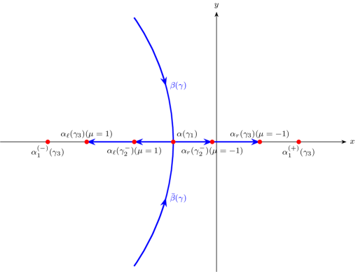
Figure 3.1: Scenario of bifurcation.

Scenario (see figure 3.1 for details):

1. Since $\alpha=0^{-}$ is an eigenvalue of $(A_{\gamma_{2}^{-}},B_{\gamma_{2}^{-}})$ and from the facts of (a) and (b), there is a complex conjugate eigenvalue pair $\{\beta(\gamma),\bar{\beta}(\gamma)\}$ of $(A_{\gamma},B_{\gamma})$ for $\gamma_{*}<\gamma<\gamma_{1}$ such that they collide at $\gamma=\gamma_{1}$ with $\alpha_{1}^{(-)}(\gamma_{1})<\alpha(\gamma_{1})=\beta(\gamma_{1})=\bar{\beta}(\gamma_{1})<0$ and bifurcate into two real eigenvalues $\alpha_{\ell}(\gamma_{1}^{+})(\mu=1)$ and $\alpha_{r}(\gamma_{1}^{+})(\mu=-1)$ with $\alpha_{\ell}(\gamma_{1}^{+})$ and $\alpha_{r}(\gamma_{1}^{+})$ moving toward the left and the right, respectively.

2. Furthermore, there exist $\gamma_{1}<\gamma_{2}^{\pm}<\gamma_{3}$ such that

   $$\alpha_{\ell}(\gamma_{2}^{\pm})(\mu=1)<\alpha(\gamma_{1})<\alpha_{r}(\gamma_{2}^{\pm})(\mu=-1)\equiv 0^{\pm}$$ (3.12)

   and

   $$0<\alpha_{r}(\gamma_{3})<\alpha_{1}^{(+)}(\gamma_{3})$$ (3.13)

   which implies that a new smallest positive eigenvalue $\alpha_{r}(\gamma_{3})$ is created at $\gamma=\gamma_{3}$.

   We now show the following cases cannot happen.

3. If there is a complex conjugate eigenvalue pair $\{\hat{\beta}(\gamma),\bar{\hat{\beta}}(\gamma)\}$ of $(A_{\gamma},B_{\gamma})$ that collides at $\gamma=\gamma_{4}>\gamma_{3}$ with

   $$0<\alpha_{r}(\gamma_{3})<\alpha_{r}(\gamma_{4})<\hat{\alpha}_{\ell}(\gamma_{4}^{+})\lesssim\hat{\alpha}(\gamma_{4})=\hat{\beta}(\gamma_{4})=\bar{\hat{\beta}}(\gamma_{4})\lesssim\hat{\alpha}_{r}(\gamma_{4}^{+}),$$ (3.14)

4. then, $\alpha_{r}(\gamma_{4})(\mu=-1)$ and $\hat{\alpha}_{\ell}(\gamma_{4}^{+})$ will collide at $\alpha_{r}(\gamma_{5})$ for $\gamma_{4}\to\gamma_{5}$ increasingly, as the combination below.

   $$\gamma=\gamma_{5}^{-}:\textbf{B-ro}(\mu=1)+\textbf{B-ro}(\mu=-1)\\ \to\gamma=\gamma_{5}:\textbf{B-re}(\mu=-1)\to\gamma=\gamma_{5}^{+}:\textbf{B-c}.$$ (3.15)

5. Then, from lemma 3.1, it follows that $p_{+}(C_{\gamma_{5}^{-}}(0^{-}))<p_{+}(C_{\gamma_{5}^{+}}(0^{-}))$, which is a contradiction.

From 3.11, lemma 3.1 and (ii), it follows that

$$p_{-}(C_{\gamma_{2}^{-}}(0^{-}))<p_{-}(C_{\gamma_{2}^{+}}(0^{-}))$$

and

$$p_{+}(C_{\gamma_{2}^{-}}(0^{+}))<p_{+}(C_{\gamma_{2}^{+}}(0^{+})).$$

This implies that the new positive and negative eigenvalues $\alpha_{r}(\gamma_{3})$ and $\alpha_{\ell}(\gamma_{3})$ must be of negative $(\mu=-1)$ and positive $(\mu=1)$ types, respectively.

On the other hand, another scenario in which the pair of eigenvalue curves $\{\beta(\gamma),\bar{\beta}(\gamma)\}$ for $\gamma_{*}<\gamma<\gamma_{1}$ collides at $\gamma=\gamma_{1}$ with

$$0<\alpha(\gamma_{1})=\beta(\gamma_{1})=\bar{\beta}(\gamma_{1})<\alpha_{1}^{(+)}(\gamma_{1})$$

can also happen (see figure 2(b) in section 4). A similar discussion as in (i)-(v) above is still held by replacing $0^{-}$ by $0^{+}$ and considering all combinations symmetric to the purely imaginary axis. These two scenarios should be mutually exclusive.

Finally, the kind of pairs in (i) and (ii) can appear as many as

$$\operatorname{rank}(U_{2})=\operatorname{rank}(\overline{\Pi_{0}}^{\operatorname{H}}(I_{3}\otimes(T^{\operatorname{H}}I^{(i)}T))\Pi_{0})$$

times because the matrix $(\varepsilon_{i}-\gamma^{2})U_{2}^{\operatorname{H}}U_{2}$ in 3.11 makes $B_{\gamma}$ change signs $\operatorname{rank}(U_{2})$ times, as $\gamma\to\infty$. ∎

4 Numerical results

(a) Schema

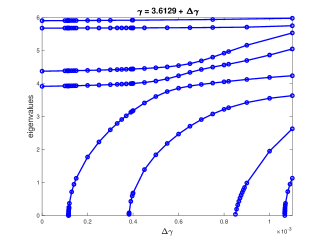
(b) Eigencurve-structure vs. various $\gamma$

Figure 4.1: A schema of 3D complex media with the FCC lattice and eigencurve-structure vs. various $\gamma$

To study numerical behaviors of the complex conjugate eigenvalue curves with $\gamma>\gamma_{*}\equiv\sqrt{\varepsilon_{i}}$, we consider the FCC lattice [7] which consists of dielectric spheres with connecting spheroids, as is shown in figure 1(a). The mesh numbers $n_{1}$, $n_{2}$ and $n_{3}$ are taken as $n_{1}=n_{2}=n_{3}=96$, and the matrix dimension of $\widehat{A}_{r}$ in 2.15b is 3,538,944. Here, $\varepsilon_{i}=13$.

As shown by the numerical results shown in [7, Figure 4], there are four newly created smallest energies as $\gamma$ increases from $\sqrt{\varepsilon_{i}}\approx 3.6056$ to $3.61397$. The zoom-in view of the eigencurve-structure is shown in figure 1(b). The results demonstrate that four newly created smallest energies are produced on the tiny increment $\Delta\gamma=10^{-3}$ of $\gamma$. These energies emerge from lower frequencies and push the original eigenmodes to higher frequencies. These new smallest eigenvalues do not collide with the original eigenvalues so no bifurcation occurs again between these eigenvalues.

In figure 4.2, we demonstrate the local behavior of the complex conjugate eigenvalue curves which collide and bifurcate into two real eigenvalues at $\gamma=\gamma_{1}\approx 3.6130162$ and $\gamma_{4}\approx 3.61396676$. The results show that the tangent lines of $\beta(\gamma)\cup\bar{\beta}(\gamma)$ and $\alpha(\gamma)\equiv\alpha_{\ell}(\gamma)\cup\alpha_{r}(\gamma)$ at $\gamma=\gamma_{1}$ and $\gamma_{4}$ are orthogonal to the real $x$- and imaginary $y$-axes, respectively, as the proof of theorem 3.7. Moreover, the complex conjugate eigenvalue curves collide and bifurcate at $\alpha(\gamma_{1})\approx-1.194\times 10^{-2}$ and $\alpha(\gamma_{4})\approx 1.693\times 10^{-2}$, respectively. The negative and positive eigenvalues $\alpha(\gamma_{1})$ and $\alpha(\gamma_{4})$ instantly move toward the right and the left, respectively, to a new positive eigenvalue $\alpha_{r}(\gamma_{1}+\Delta\gamma_{1})$ and a negative eigenvalue $\alpha_{\ell}(\gamma_{4}+\Delta\gamma_{4})$ along the real axis, where $\Delta\gamma_{1}=6\times 10^{-9}$ and $\Delta\gamma_{4}=2\times 10^{-8}$.

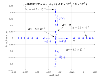
(a) The first newly created smallest energy

(b) The fourth newly created smallest energy

Figure 4.2: The local behavior of the complex conjugate eigenvalue curves which collide and bifurcate into two real eigenvalues at $\gamma\approx 3.6130162$ and $3.61396676$.

5 Conclusions

In this paper, we prove a detailed bifurcation analysis of eigenstructures of the discrete single-curl operator in 3D Maxwell’s equations with Pasteur media that depend on a chirality parameter $\gamma$ as it varies. We compensate for the theoretical difficulties and guarantee that the numerical results are valid and reliable. These results can provide an important theoretical viewpoint on numerical computations, especially regarding the support of numerical results in [7] computed by the developed SIRA + MINRES for NFGEP. It is worth mentioning that in remark 3.1, we show that the associated electric field $\boldsymbol{e}$ of the defective infinite eigenvalue is zero outside the material. This provides a very good reason to explain that the electric field corresponding to the newly created smallest energy state is almost concentrated in the material such that only a small amount of the field leak into the background material.

In the future, it would be very challenging to compute the Bloch dispersion curves corresponding to a periodic array of plasmonic nanoparticles inside a chiral background medium.

Appendix A The regularity of $A-\omega B$

Theorem A.1.

$A-\omega B$ is always regular, as long as three line segments, parallel to the three mesh grid axes respectively, with end points lying on the boundary of the mesh grid are outside the medium, i.e., there exist some $i_{1},i_{1}^{\prime}\in[1,n_{1}],i_{2},i_{2}^{\prime}\in[1,n_{2}],i_{3},i_{3}^{\prime}\in[1,n_{3}]$, such that $\mathcal{G}\subset\operatorname{\mathcal{D}}_{o}$, where $\mathcal{G}=\mathcal{G}_{1}\cup\mathcal{G}_{2}\cup\mathcal{G}_{3}$ with $\mathcal{G}_{1}=\{\langle i,i_{2},i_{3}^{\prime}\rangle:i\in\mathbb{Z}\}$, $\mathcal{G}_{2}=\{\langle i_{1}^{\prime},i,i_{3}\rangle:i\in\mathbb{Z}\}$, $\mathcal{G}_{3}=\{\langle i_{1},i_{2}^{\prime},i\rangle:i\in\mathbb{Z}\}$.

Proof.

First, we will observe $\mathcal{S}$. To address it, we have to discuss several cases.

Case I. $\Lambda_{\ell},\ell=1,2,3$ are nonsingular. The only proper $z_{1},z_{2},z_{3}$ are all zero.

First, 3.2a has nontrivial solutions if and only if there exists $i_{\ell}\in[1,n_{\ell}],\ell=1,2,3$, such that

$$\eta_{n_{3}}^{\boldsymbol{k}\cdot\widehat{\boldsymbol{a}}_{3}+i_{3}}\eta_{n_{2}n_{3}}^{-m_{2}i_{2}}\eta_{n_{1}n_{3}}^{-\widehat{m}_{1}i_{1}}\eta_{n_{1}n_{2}n_{3}}^{m_{1}m_{2}i_{1}}=\eta_{n_{2}}^{\boldsymbol{k}\cdot\widehat{\boldsymbol{a}}_{2}+i_{2}}\eta_{n_{1}n_{2}}^{-m_{1}i_{1}}=\eta_{n_{1}}^{\boldsymbol{k}\cdot\widehat{\boldsymbol{a}}_{1}+i_{1}},$$

and in this case, the $\langle i_{1},i_{2},i_{3}\rangle$-th entry of $x_{1}$ is nonzero. It is equivalent to

$$\frac{i_{1}+\boldsymbol{k}\cdot\widehat{\boldsymbol{a}}_{1}}{n_{1}}-s_{1} =\frac{i_{2}+\boldsymbol{k}\cdot\widehat{\boldsymbol{a}}_{2}-\frac{m_{1}}{n_{1}}i_{1}}{n_{2}}-s_{2}$$

$$=\frac{i_{3}+\boldsymbol{k}\cdot\widehat{\boldsymbol{a}}_{3}-\frac{m_{2}}{n_{2}}i_{2}-\frac{\widehat{m}_{1}}{n_{1}}i_{1}+\frac{m_{1}m_{2}}{n_{1}n_{2}}i_{1}}{n_{3}}-s_{3}=:\lambda\in[0,1),$$

for some $s_{1},s_{2},s_{3}\in\mathbb{Z}$. In other words, $x_{1}=I^{\mathcal{I}_{0}}x_{1}$, where

$$\mathcal{I}_{0}:=\{\langle\lambda\widehat{n}_{1}-\kappa_{1},\lambda\widehat{n}_{2}-\kappa_{2},\lambda\widehat{n}_{3}-\kappa_{3}\rangle:\lambda\widehat{n}_{\ell}-\kappa_{\ell}\in\mathbb{Z},0<\lambda<1\},$$

with

$$\widehat{n}_{1} =n_{1},\quad \kappa_{1} =\boldsymbol{k}\cdot\boldsymbol{a}_{1},$$

$$\widehat{n}_{2} =n_{2}+m_{1},\quad \kappa_{2} =\boldsymbol{k}\cdot(\boldsymbol{a}_{2}+\rho_{1}\boldsymbol{a}_{1})-m_{1}s_{1},$$

$$\widehat{n}_{3} =n_{3}+m_{2}+\widehat{m}_{1},\quad \kappa_{3} =\boldsymbol{k}\cdot(\boldsymbol{a}_{3}+\rho_{2}\boldsymbol{a}_{2}+\widehat{\rho}_{1}\boldsymbol{a}_{1})-m_{2}s_{2}-\widehat{m}_{1}s_{1}.$$

Clearly, $x_{1}\neq 0$ is equivalent to $(I^{\mathcal{I}_{0}}_{\sigma})^{\operatorname{T}}x_{1}\neq 0$. Moreover, if $\mathcal{I}_{0}\neq\emptyset$, then it can be shown that

$$\mathcal{I}_{0}=\{\langle\lambda\widehat{n}_{1}-\kappa_{1},\lambda\widehat{n}_{2}-\kappa_{2},\lambda\widehat{n}_{3}-\kappa_{3}\rangle:\lambda=\lambda_{0}+\frac{p}{\widehat{n}_{123}},p\in[0,\widehat{n}_{123})\cap\mathbb{Z}\},$$

with $\lambda_{0}\in[0,\frac{1}{\widehat{n}_{123}})$ satisfying $\lambda_{0}\widehat{n}_{\ell}-\kappa_{\ell}\in\mathbb{Z}$, and $\widehat{n}_{123}=\gcd(\widehat{n}_{1},\widehat{n}_{2},\widehat{n}_{3})$, the greatest common divisor of $\widehat{n}_{1}$, $\widehat{n}_{2}$ and $\widehat{n}_{3}$. Note that $\lambda_{0}$ here is unique, and $|\mathcal{I}_{0}|=\widehat{n}_{123}$.

Then, consider 3.2b, namely, solving $I^{(o)}T\Lambda_{1}x_{1}=0$. For ease, we mainly discuss the case that the related index sets are nonempty. Inserting the solution of 3.2a into 3.2b, we have

$$0=I^{(o)}T\Lambda_{1}x_{1}=I^{(o)}T\Lambda_{1}I^{\mathcal{I}_{0}}x_{1}=I^{(o)}TI^{\mathcal{I}_{0}}\Lambda_{1}x_{1}=I^{(o)}TI^{\mathcal{I}_{0}}_{\sigma}[(I^{\mathcal{I}_{0}}_{\sigma})^{\operatorname{T}}\Lambda_{1}x_{1}].$$

Recall the form of $T=[t_{\ell}]$ in 2.6. Write

$$U_{\widehat{n}_{123}}=[u_{\widehat{n}_{123},p}]_{p=1,\dots,\widehat{n}_{123}},\qquad u_{\widehat{n}_{123},p}:=V_{n_{3}}(\eta_{\widehat{n}_{123}}^{p})\otimes V_{n_{2}}(\eta_{\widehat{n}_{123}}^{p})\otimes V_{n_{1}}(\eta_{\widehat{n}_{123}}^{p}).$$

and $t_{0}=t_{\langle\lambda_{0}\widehat{n}_{1}-\kappa_{1},\lambda_{0}\widehat{n}_{2}-\kappa_{2},\lambda_{0}\widehat{n}_{3}-\kappa_{3}\rangle}$. It can be seen that

$$t_{\langle(\lambda_{0}+\frac{p}{\widehat{n}_{123}})\widehat{n}_{1}-\kappa_{1},(\lambda_{0}+\frac{p}{\widehat{n}_{123}})\widehat{n}_{2}-\kappa_{2},(\lambda_{0}+\frac{p}{\widehat{n}_{123}})\widehat{n}_{3}-\kappa_{3}\rangle}=\operatorname{diag}(u_{\widehat{n}_{123},p})t_{0}=\operatorname{diag}(t_{0})u_{\widehat{n}_{123},p},$$

and then $TI^{\mathcal{I}_{0}}_{\sigma}=\operatorname{diag}(t_{0})U_{\widehat{n}_{123}}$. Thus,

$$0 =I^{(o)}TI^{\mathcal{I}_{0}}_{\sigma}[(I^{\mathcal{I}_{0}}_{\sigma})^{\operatorname{T}}\Lambda_{1}x_{1}]$$

$$=I^{(o)}\operatorname{diag}(t_{0})U_{\widehat{n}_{123}}[(I^{\mathcal{I}_{0}}_{\sigma})^{\operatorname{T}}\Lambda_{1}x_{1}]$$

$$=\operatorname{diag}(t_{0})I^{(o)}U_{\widehat{n}_{123}}[(I^{\mathcal{I}_{0}}_{\sigma})^{\operatorname{T}}\Lambda_{1}I^{\mathcal{I}_{0}}_{\sigma}][(I^{\mathcal{I}_{0}}_{\sigma})^{\operatorname{T}}x_{1}].$$

Noticing that each entry of $t_{0}$ is nonzero, and $(I^{\mathcal{I}_{0}}_{\sigma})^{\operatorname{T}}\Lambda_{1}I^{\mathcal{I}_{0}}_{\sigma}$ is nonsingular, $\mathcal{S}=\{0\}$ is equivalent to $I^{(o)}U_{\widehat{n}_{123}}x=0$ has only trivial solutions, namely, $I^{(o)}U_{\widehat{n}_{123}}$ is of full column rank.

Case II-1. $\Lambda_{\ell},\ell=2,3$ are nonsingular, but $\Lambda_{1}$ is singular. By the form of $\Lambda_{1}$ in 2.5,

$$\Lambda_{1} \Leftrightarrow \frac{i_{1}+\boldsymbol{k}\cdot\widehat{\boldsymbol{a}}_{1}}{n_{1}}\in\mathbb{Z} i_{1} \Leftrightarrow\boldsymbol{k}\cdot\widehat{\boldsymbol{a}}_{1}=0$$ is singular for some ,

and for the case $i_{1}=n_{1}$. The only proper $z_{2},z_{3}$ are both zero.

First, 3.2a has nontrivial solutions, if and only if:

1. there exists $i_{\ell}\in[1,n_{\ell}],\ell=1,2,3$, $i_{1}\neq n_{1}$, such that

   $$\frac{i_{1}+\boldsymbol{k}\cdot\widehat{\boldsymbol{a}}_{1}}{n_{1}}-s_{1} =\frac{i_{2}+\boldsymbol{k}\cdot\widehat{\boldsymbol{a}}_{2}-\frac{m_{1}}{n_{1}}i_{1}}{n_{2}}-s_{2}$$

   $$=\frac{i_{3}+\boldsymbol{k}\cdot\widehat{\boldsymbol{a}}_{3}-\frac{m_{2}}{n_{2}}i_{2}-\frac{\widehat{m}_{1}}{n_{1}}i_{1}+\frac{m_{1}m_{2}}{n_{1}n_{2}}i_{1}}{n_{3}}-s_{3}=:\lambda\in[0,1),$$

   for some $s_{1},s_{2},s_{3}\in\mathbb{Z}$. For the case, the $\langle i_{1},i_{2},i_{3}\rangle$-th entry of $x_{1}$ is nonzero.

2. there exists $i_{\ell}\in[1,n_{\ell}],\ell=2,3$, such that

   $$\frac{i_{2}+\boldsymbol{k}\cdot\widehat{\boldsymbol{a}}_{2}-\frac{m_{1}}{n_{1}}n_{1}}{n_{2}}-s_{2}\\ =\frac{i_{3}+\boldsymbol{k}\cdot\widehat{\boldsymbol{a}}_{3}-\frac{m_{2}}{n_{2}}i_{2}-\frac{\widehat{m}_{1}}{n_{1}}n_{1}+\frac{m_{1}m_{2}}{n_{1}n_{2}}n_{1}}{n_{3}}-s_{3}=:\lambda\in[0,1),$$

   for some $s_{1},s_{2},s_{3}\in\mathbb{Z}$. For the case, the $\langle n_{1},i_{2},i_{3}\rangle$-th entry of $x_{1}$ is decided by $z_{1}$, where $z_{1}\in\operatorname{\mathcal{R}}(I^{\mathcal{I}_{1}}_{\sigma})$, and

   $$\mathcal{I}_{1} :=\{\langle n_{1},\lambda\widehat{n}_{2}-\kappa_{2},\lambda\widehat{n}_{3}-\kappa_{3}\rangle:\lambda\widehat{n}_{\ell}-\kappa_{\ell}\in\mathbb{Z},0<\lambda<1\}$$

   $$=\{\langle n_{1},\lambda\widehat{n}_{2}-\kappa_{2},\lambda\widehat{n}_{3}-\kappa_{3}\rangle:\lambda=\lambda_{1}+\frac{p}{\widehat{n}_{23}},p\in[0,\widehat{n}_{23})\cap\mathbb{Z}\},$$

   and

   $$\widehat{n}_{2} =n_{2},\quad \kappa_{2} =\boldsymbol{k}\cdot(\boldsymbol{a}_{2}+\rho_{1}\boldsymbol{a}_{1})-m_{1},$$

   $$\widehat{n}_{3} =n_{3}+m_{2},\quad \kappa_{3} =\boldsymbol{k}\cdot(\boldsymbol{a}_{3}+\rho_{2}\boldsymbol{a}_{2}+\widehat{\rho}_{1}\boldsymbol{a}_{1})-m_{2}s_{2}-\widehat{m}_{1}.$$

   In detail, $(I^{\mathcal{I}_{1}}_{\sigma})^{\operatorname{H}}x_{1}=-\delta_{2}[(I^{\mathcal{I}_{1}}_{\sigma})^{\operatorname{H}}\Lambda_{2}I^{\mathcal{I}_{1}}_{\sigma}]^{-1}(I^{\mathcal{I}_{1}}_{\sigma})^{\operatorname{H}}z_{1}$.

In other words, $x_{1}=I^{\mathcal{I}_{0}\cup\mathcal{I}_{1}}x_{1}$. Moreover, if $\mathcal{I}_{1}\neq\emptyset$, with $\lambda_{1}\in[0,\frac{1}{\widehat{n}_{23}})$ satisfying $\lambda_{0}\widehat{n}_{\ell}-\kappa_{\ell}\in\mathbb{Z}$, and $\widehat{n}_{23}=\gcd(\widehat{n}_{2},\widehat{n}_{3})$. Note that $\lambda_{1}$ here is unique, and $|\mathcal{I}_{1}|=\widehat{n}_{23}$. Clearly, $x_{1}\neq 0$ is equivalent to $(I^{\mathcal{I}_{0}\cup\mathcal{I}_{1}}_{\sigma})^{\operatorname{T}}x_{1}\neq 0$.

Then, consider 3.1 and 3.2b, namely, solving $I^{(o)}T\Lambda_{1}x_{1}=0,I^{(o)}Tz_{1}=0$. For ease, we mainly discuss the case in which the related index sets are nonempty. Inserting the solution of 3.2a into 3.2b, we have

$$0=\begin{bmatrix}I^{(o)}T\Lambda_{1}x_{1}\\ I^{(o)}Tz_{1}\\ \end{bmatrix}=\begin{bmatrix}I^{(o)}T\Lambda_{1}I^{\mathcal{I}_{0}}x_{1}\\ I^{(o)}TI^{\mathcal{I}_{1}}z_{1}\\ \end{bmatrix} =\begin{bmatrix}I^{(o)}TI^{\mathcal{I}_{0}}_{\sigma}[(I^{\mathcal{I}_{0}}_{\sigma})^{\operatorname{T}}\Lambda_{1}x_{1}]\\ I^{(o)}TI^{\mathcal{I}_{1}}_{\sigma}[(I^{\mathcal{I}_{1}}_{\sigma})^{\operatorname{T}}z_{1}]\\ \end{bmatrix}$$

$$=\begin{bmatrix}I^{(o)}TI^{\mathcal{I}_{0}}_{\sigma}&\\ &I^{(o)}TI^{\mathcal{I}_{1}}_{\sigma}\\ \end{bmatrix}\begin{bmatrix}(I^{\mathcal{I}_{0}}_{\sigma})^{\operatorname{T}}\Lambda_{1}x_{1}\\ (I^{\mathcal{I}_{1}}_{\sigma})^{\operatorname{T}}z_{1}\\ \end{bmatrix}.$$

Similarly, $\mathcal{S}=\{0\}$ is equivalent to $\begin{bmatrix}I^{(o)}U_{\widehat{n}_{123}}&\\ &I^{(o)}U_{\widehat{n}_{23}}\\ \end{bmatrix}$ is of full column rank, where

$$U_{\widehat{n}_{23}}=[u_{\widehat{n}_{23},p}]_{p=1,\dots,\widehat{n}_{23}},\qquad u_{\widehat{n}_{13},p}:=V_{n_{3}}(\eta_{\widehat{n}_{23}}^{p})\otimes V_{n_{2}}(\eta_{\widehat{n}_{13}}^{p})\otimes V_{n_{1}}(1).$$

Case II-2. $\Lambda_{\ell},\ell=1,3$ are nonsingular, but $\Lambda_{2}$ is singular. By the form of $\Lambda_{2}$ in 2.5, we have:

1. $m_{1}=0$:

   $$\Lambda_{2} \Leftrightarrow \frac{i_{2}+\boldsymbol{k}\cdot\widehat{\boldsymbol{a}}_{2}}{n_{2}}\in\mathbb{Z} i_{2} \Leftrightarrow\boldsymbol{k}\cdot\widehat{\boldsymbol{a}}_{2}=0$$ is singular for some ,

   and everything is similar to Case II-1. $\mathcal{S}=\{0\}$ is equivalent to the matrix $\begin{bmatrix}I^{(o)}U_{\widehat{n}_{123}}&\\ &I^{(o)}U_{\widehat{n}_{13}}\\ \end{bmatrix}$ is of full column rank, where

   $$U_{\widehat{n}_{13}}=[u_{\widehat{n}_{13},p}]_{p=1,\dots,\widehat{n}_{13}},\qquad u_{\widehat{n}_{13},p}:=V_{n_{3}}(\eta_{\widehat{n}_{13}}^{p})\otimes V_{n_{2}}(1)\otimes V_{n_{1}}(\eta_{\widehat{n}_{13}}^{p}).$$

2. $m_{1}\neq 0$:

   $$\Lambda_{2} \Leftrightarrow\text{$\frac{i_{2}+\boldsymbol{k}\cdot\widehat{\boldsymbol{a}}_{2}-\frac{m_{1}}{n_{1}}i_{1}}{n_{2}}\in\mathbb{Z}$ for some $i_{1},i_{2}$}$$ is singular

   $$\Leftrightarrow\widetilde{n}_{2}:=\frac{n_{1}}{m_{1}}\boldsymbol{k}\cdot\widehat{\boldsymbol{a}}_{2}\in\mathbb{Z},$$

   and for the case $i_{1}=\widetilde{n}_{2},i_{2}=n_{2}$. The only proper $z_{1},z_{3}$ are both zero.

   First, 3.2a has nontrivial solutions, if and only if:

   1. there exists $i_{\ell}\in[1,n_{\ell}],\ell=1,2,3$, $(i_{1},i_{2})\neq(\widetilde{n}_{2},n_{2})$, such that

      $$\!\!\!\!\!\frac{i_{1}+\boldsymbol{k}\cdot\widehat{\boldsymbol{a}}_{1}}{n_{1}}-s_{1} =\frac{i_{2}+\boldsymbol{k}\cdot\widehat{\boldsymbol{a}}_{2}-\frac{m_{1}}{n_{1}}i_{1}}{n_{2}}-s_{2}$$

      $$=\frac{i_{3}+\boldsymbol{k}\cdot\widehat{\boldsymbol{a}}_{3}-\frac{m_{2}}{n_{2}}i_{2}-\frac{\widehat{m}_{1}}{n_{1}}i_{1}+\frac{m_{1}m_{2}}{n_{1}n_{2}}i_{1}}{n_{3}}-s_{3}=:\lambda\in[0,1),$$

      for some $s_{1},s_{2},s_{3}\in\mathbb{Z}$. For the case, the $\langle i_{1},i_{2},i_{3}\rangle$-th entry of $x_{1}$ is nonzero.

   2. $(i_{1},i_{2})=(\widetilde{n}_{2},n_{2})$. For the case, the $\langle\widetilde{n}_{2},n_{2},i_{3}\rangle$-th entry of $x_{1}$ is decided by $z_{2}$, where $z_{2}\in\operatorname{\mathcal{R}}(I^{\mathcal{I}_{2}^{m}}_{\sigma})$, and

      $$\mathcal{I}_{2}^{m} :=\{\langle\widetilde{n}_{2},n_{2},i_{3}\rangle\}.$$

      In detail, $(I^{\mathcal{I}_{2}^{m}}_{\sigma})^{\operatorname{H}}x_{1}=-\delta_{3}[(I^{\mathcal{I}_{2}^{m}}_{\sigma})^{\operatorname{H}}\Lambda_{3}I^{\mathcal{I}_{2}^{m}}_{\sigma}]^{-1}(I^{\mathcal{I}_{2}^{m}}_{\sigma})^{\operatorname{H}}z_{2}$.

   In other words, $x_{1}=I^{\mathcal{I}_{0}\cup\mathcal{I}_{2}^{m}}x_{1}$. Note that $|\mathcal{I}_{2}^{m}|=n_{3}$. Clearly, $x_{1}\neq 0$ is equivalent to $(I^{\mathcal{I}_{0}\cup\mathcal{I}_{2}^{m}}_{\sigma})^{\operatorname{T}}x_{1}\neq 0$.

   Then, consider 3.1 and 3.2b, namely, solving $I^{(o)}T\Lambda_{1}x_{1}=0,I^{(o)}Tz_{2}=0$. The steps proceed similarly to Case II-1. $\mathcal{S}=\{0\}$ is equivalent to $\begin{bmatrix}I^{(o)}U_{\widehat{n}_{123}}&\\ &I^{(o)}U_{n_{3}}\\ \end{bmatrix}$ is of full column rank, where

   $$U_{n_{3}}=[u_{n_{3},p}]_{p=1,\dots,n_{3}},\qquad u_{n_{3},p}:=V_{n_{3}}(\eta_{n_{3}}^{p})\otimes V_{n_{2}}(1)\otimes V_{n_{1}}(1).$$

Case II-3. $\Lambda_{\ell},\ell=1,2$ are nonsingular, but $\Lambda_{3}$ is singular. By the form of $\Lambda_{3}$ in 2.5, we have:

1. $\widehat{m}_{1}=0,m_{2}=0$:

   $$\Lambda_{3} \Leftrightarrow\text{$\frac{i_{3}+\boldsymbol{k}\cdot\widehat{\boldsymbol{a}}_{3}}{n_{2}}\in\mathbb{Z}$ for some $i_{3}$}$$ is singular

   $$\Leftrightarrow\boldsymbol{k}\cdot\widehat{\boldsymbol{a}}_{3}=0,$$

   and everything is similar to Case II-1. $\mathcal{S}=\{0\}$ is equivalent to the matrix $\begin{bmatrix}I^{(o)}U_{\widehat{n}_{123}}&\\ &I^{(o)}U_{\widehat{n}_{12}}\\ \end{bmatrix}$ is of full column rank, where

   $$U_{\widehat{n}_{12}}=[u_{\widehat{n}_{12},p}]_{p=1,\dots,\widehat{n}_{12}},\qquad u_{\widehat{n}_{12},p}:=V_{n_{3}}(1)\otimes V_{n_{2}}(\eta_{\widehat{n}_{12}}^{p})\otimes V_{n_{1}}(\eta_{\widehat{n}_{12}}^{p}).$$

2. $\widehat{m}_{1}\neq 0,m_{2}=0$:

   $$\Lambda_{3} \Leftrightarrow\text{$\frac{i_{3}+\boldsymbol{k}\cdot\widehat{\boldsymbol{a}}_{3}-\frac{\widehat{m}_{1}}{n_{1}}i_{1}}{n_{3}}\in\mathbb{Z}$ for some $i_{1},i_{3}$}$$ is singular

   $$\Leftrightarrow\widetilde{n}_{3,1}:=\frac{n_{1}}{\widehat{m}_{1}}\boldsymbol{k}\cdot\widehat{\boldsymbol{a}}_{3}\in\mathbb{Z},$$

   and everything is similar to Case II-2(2). $\mathcal{S}=\{0\}$ is equivalent to the matrix $\begin{bmatrix}I^{(o)}U_{\widehat{n}_{123}}&\\ &I^{(o)}U_{n_{2}}\\ \end{bmatrix}$ is of full column rank, where

   $$U_{n_{2}}=[u_{n_{2},p}]_{p=1,\dots,n_{2}},\qquad u_{n_{2},p}:=V_{n_{3}}(1)\otimes V_{n_{2}}(\eta_{n_{2}}^{p})\otimes V_{n_{1}}(1).$$

3. $m_{2}\neq 0,\widehat{m}_{1}=0,m_{1}=0$:

   $$\Lambda_{3} \Leftrightarrow\text{$\frac{i_{3}+\boldsymbol{k}\cdot\widehat{\boldsymbol{a}}_{3}-\frac{m_{2}}{n_{2}}i_{2}}{n_{3}}\in\mathbb{Z}$ for some $i_{2},i_{3}$}$$ is singular

   $$\Leftrightarrow\widetilde{n}_{3,2}:=\frac{n_{1}}{\widehat{m}_{1}}\boldsymbol{k}\cdot\widehat{\boldsymbol{a}}_{3}\in\mathbb{Z},$$

   and everything is similar to Case II-2(2). $\mathcal{S}=\{0\}$ is equivalent to the matrix $\begin{bmatrix}I^{(o)}U_{\widehat{n}_{123}}&\\ &I^{(o)}U_{\widehat{n}_{1}}\\ \end{bmatrix}$ is of full column rank, where

   $$U_{n_{1}}=[u_{n_{1},p}]_{p=1,\dots,n_{1}},\qquad u_{n_{1},p}:=V_{n_{3}}(1)\otimes V_{n_{2}}(1)\otimes V_{n_{1}}(\eta_{n_{1}}^{p}).$$

4. $m_{2}\neq 0$, $\widehat{m}_{1},m_{1}$ not both zero:

   $$\!\!\!\text{ $\Lambda_{3}$ is singular }\Leftrightarrow\text{$\frac{i_{3}+\boldsymbol{k}\cdot\widehat{\boldsymbol{a}}_{3}-\frac{m_{2}}{n_{2}}i_{2}-\frac{\widehat{m}_{1}}{n_{1}}i_{1}+\frac{m_{1}m_{2}}{n_{1}n_{2}}i_{1}}{n_{3}}\in\mathbb{Z}$ for some $i_{1},i_{2},i_{3}$},$$

   and for the case where there is only one choice $(i_{1},i_{2},i_{3})$. Write the single-element set as $\mathcal{I}_{3}^{m}$. The only proper $z_{1},z_{2}$ are both zero.

   First, 3.2a has nontrivial solutions, if and only if:

   1. there exists $i_{\ell}\in[1,n_{\ell}],\ell=1,2,3$, $(i_{1},i_{2},i_{3})\notin\mathcal{I}_{3}^{m}$, such that

      $$\!\!\!\!\!\frac{i_{1}+\boldsymbol{k}\cdot\widehat{\boldsymbol{a}}_{1}}{n_{1}}-s_{1} =\frac{i_{2}+\boldsymbol{k}\cdot\widehat{\boldsymbol{a}}_{2}-\frac{m_{1}}{n_{1}}i_{1}}{n_{2}}-s_{2}$$

      $$=\frac{i_{3}+\boldsymbol{k}\cdot\widehat{\boldsymbol{a}}_{3}-\frac{m_{2}}{n_{2}}i_{2}-\frac{\widehat{m}_{1}}{n_{1}}i_{1}+\frac{m_{1}m_{2}}{n_{1}n_{2}}i_{1}}{n_{3}}-s_{3}=:\lambda\in[0,1),$$

      for some $s_{1},s_{2},s_{3}\in\mathbb{Z}$. For the case, the $\langle i_{1},i_{2},i_{3}\rangle$-th entry of $x_{1}$ is nonzero.

   2. $(i_{1},i_{2},i_{3})\in\mathcal{I}_{3}^{m}$. For the case, the $\langle\widetilde{n}_{2},n_{2},i_{3}\rangle$-th entry of $x_{1}$ is decided by $z_{3}$, where $z_{2}\in\operatorname{\mathcal{R}}(I^{\mathcal{I}_{3}^{m}}_{\sigma})$. In detail,

      $$(I^{\mathcal{I}_{3}^{m}}_{\sigma})^{\operatorname{H}}x_{1}=-\delta_{3}[(I^{\mathcal{I}_{3}^{m}}_{\sigma})^{\operatorname{H}}\Lambda_{3}I^{\mathcal{I}_{3}^{m}}_{\sigma}]^{-1}(I^{\mathcal{I}_{3}^{m}}_{\sigma})^{\operatorname{H}}z_{3}.$$

   In other words, $x_{1}=I^{\mathcal{I}_{0}\cup\mathcal{I}_{3}^{m}}x_{1}$. Note that $|\mathcal{I}_{3}^{m}|=n_{1}$. Clearly, $x_{1}\neq 0$ is equivalent to $(I^{\mathcal{I}_{0}\cup\mathcal{I}_{3}^{m}}_{\sigma})^{\operatorname{T}}x_{1}\neq 0$.

   Then, consider 3.1 and 3.2b, namely, solving $I^{(o)}T\Lambda_{1}x_{1}=0,I^{(o)}Tz_{3}=0$. The steps proceed similarly to Case II-1. $\mathcal{S}=\{0\}$ is equivalent to $\begin{bmatrix}I^{(o)}U_{\widehat{n}_{123}}&\\ &I^{(o)}U_{1}\\ \end{bmatrix}$ is of full column rank, where

   $$U_{1}=[u_{1,1}],\qquad u_{1,1}:=V_{n_{3}}(1)\otimes V_{n_{2}}(1)\otimes V_{n_{1}}(1).$$

Case III-3. $\Lambda_{\ell},\ell=1,2$ are singular, but $\Lambda_{3}$ is nonsingular. The only proper $z_{3}=0$. By the form of $\Lambda_{1},\Lambda_{2}$ in 2.5, we have:

1. $m_{1}=0$: it is similar to the combination of Case II-1 and Case II-2(1).

   $$\Lambda_{1} \Leftrightarrow \frac{i_{1}+\boldsymbol{k}\cdot\widehat{\boldsymbol{a}}_{1}}{n_{1}}\in\mathbb{Z} i_{1} \Leftrightarrow\boldsymbol{k}\cdot\widehat{\boldsymbol{a}}_{1}=0$$ is singular for some ,

   $$\Lambda_{2} \Leftrightarrow \frac{i_{2}+\boldsymbol{k}\cdot\widehat{\boldsymbol{a}}_{2}}{n_{2}}\in\mathbb{Z} i_{2} \Leftrightarrow\boldsymbol{k}\cdot\widehat{\boldsymbol{a}}_{2}=0$$ is singular for some .

   In detail,

   $$(I^{\mathcal{I}_{1}}_{\sigma})^{\operatorname{H}}x_{1}=-\delta_{3}[(I^{\mathcal{I}_{1}}_{\sigma})^{\operatorname{H}}\Lambda_{3}I^{\mathcal{I}_{1}}_{\sigma}]^{-1}(I^{\mathcal{I}_{1}}_{\sigma})^{\operatorname{H}}z_{1},$$

   and

   $$(I^{\mathcal{I}_{2}}_{\sigma})^{\operatorname{H}}x_{1}=-\delta_{3}[(I^{\mathcal{I}_{2}}_{\sigma})^{\operatorname{H}}\Lambda_{3}I^{\mathcal{I}_{2}}_{\sigma}]^{-1}(I^{\mathcal{I}_{2}}_{\sigma})^{\operatorname{H}}z_{2}.$$

   This forces $(I^{\mathcal{I}_{1}\cap\mathcal{I}_{2}}_{\sigma})^{\operatorname{H}}z_{1}=(I^{\mathcal{I}_{1}\cap\mathcal{I}_{2}}_{\sigma})^{\operatorname{H}}z_{2}$.

   Then, consider 3.1 and 3.2b, namely, solving $I^{(o)}T\Lambda_{1}x_{1}=0,I^{(o)}Tz_{1}=0,I^{(o)}Tz_{2}=0$. For ease, we mainly discuss the case in which the related index sets are nonempty. Inserting the solution of 3.2a into 3.2b, we have

   $$0=\begin{bmatrix}I^{(o)}T\Lambda_{1}x_{1}\\ I^{(o)}Tz_{1}\\ I^{(o)}Tz_{2}\\ (I^{\mathcal{I}_{1}\cap\mathcal{I}_{2}}_{\sigma})^{\operatorname{H}}(z_{1}-z_{2})\\ \end{bmatrix}=\begin{bmatrix}I^{(o)}TI^{\mathcal{I}_{0}}_{\sigma}[(I^{\mathcal{I}_{0}}_{\sigma})^{\operatorname{T}}\Lambda_{1}x_{1}]\\ I^{(o)}TI^{\mathcal{I}_{1}}_{\sigma}[(I^{\mathcal{I}_{1}}_{\sigma})^{\operatorname{T}}z_{1}]\\ I^{(o)}TI^{\mathcal{I}_{2}}_{\sigma}[(I^{\mathcal{I}_{2}}_{\sigma})^{\operatorname{T}}z_{2}]\\ (I^{\mathcal{I}_{1}\cap\mathcal{I}_{2}}_{\sigma})^{\operatorname{H}}(z_{1}-z_{2})\\ \end{bmatrix}=\widetilde{T}\begin{bmatrix}(I^{\mathcal{I}_{0}}_{\sigma})^{\operatorname{T}}\Lambda_{1}x_{1}\\ (I^{\mathcal{I}_{1}\setminus\mathcal{I}_{2}}_{\sigma})^{\operatorname{T}}z_{1}\\ (I^{\mathcal{I}_{1}\cap\mathcal{I}_{2}}_{\sigma})^{\operatorname{T}}z_{1}\\ (I^{\mathcal{I}_{2}\setminus\mathcal{I}_{1}}_{\sigma})^{\operatorname{T}}z_{2}\\ (I^{\mathcal{I}_{1}\cap\mathcal{I}_{2}}_{\sigma})^{\operatorname{T}}z_{2}\\ \end{bmatrix},$$

   where $\widetilde{T}=\!\begin{bmatrix}I^{(o)}TI^{\mathcal{I}_{0}}_{\sigma}&&&&\\ &I^{(o)}TI^{\mathcal{I}_{1}\setminus\mathcal{I}_{2}}_{\sigma}&I^{(o)}TI^{\mathcal{I}_{1}\cap\mathcal{I}_{2}}_{\sigma}&&\\ &&&I^{(o)}TI^{\mathcal{I}_{2}\setminus\mathcal{I}_{1}}_{\sigma}&I^{(o)}TI^{\mathcal{I}_{1}\cap\mathcal{I}_{2}}_{\sigma}\\ &&I&&-I\\ \end{bmatrix}$. This equation has only trivial solutions, as long as $\begin{bmatrix}I^{(o)}TI^{\mathcal{I}_{0}}_{\sigma}&&\\ &I^{(o)}TI^{\mathcal{I}_{1}}_{\sigma}&\\ &&I^{(o)}TI^{\mathcal{I}_{2}}_{\sigma}\\ \end{bmatrix}$ is of full column rank. Thus $\mathcal{S}=\{0\}$, as long as $\begin{bmatrix}I^{(o)}U_{\widehat{n}_{123}}&&\\ &I^{(o)}U_{\widehat{n}_{23}}&\\ &&I^{(o)}U_{\widehat{n}_{13}}\\ \end{bmatrix}$ is of full column rank.

2. $m_{1}\neq 0$: it is similar to Case III-3(1), considering the combination of Case II-1 and Case II-2(2). Thus $\mathcal{S}=\{0\}$, as long as $\!\begin{bmatrix}I^{(o)}U_{\widehat{n}_{123}}&&\\ &I^{(o)}U_{\widehat{n}_{23}}&\\ &&I^{(o)}U_{\widehat{n}_{3}}\\ \end{bmatrix}$ is of full column rank.

Case III-2. $\Lambda_{\ell},\ell=1,3$ are singular, but $\Lambda_{2}$ is nonsingular. It is similar to Case III-1, considering the combination of Case II-1 and Case II-3,

Case III-1.. $\Lambda_{\ell},\ell=2,3$ are singular, but $\Lambda_{1}$ is nonsingular. It is similar to Case III-1, considering the combination of Case II-2 and Case II-3.

Case IV. $\Lambda_{\ell},\ell=1,2,3$ are all singular.

1. $m_{1}=0,\widehat{m}_{1}=0,m_{2}=0$: it is similar to Case III-1(1), considering the combination of Case II-1, Case II-2 and Case II-3. Since $\Lambda_{q}=\Lambda_{1}^{\operatorname{H}}\Lambda_{1}+\Lambda_{2}^{\operatorname{H}}\Lambda_{2}+\Lambda_{3}^{\operatorname{H}}\Lambda_{3}\succ 0$, we know $\mathcal{I}_{1}\cap\mathcal{I}_{2}\cap\mathcal{I}_{3}=\emptyset$. Note that $(I^{\mathcal{I}_{1}\cap\mathcal{I}_{2}}_{\sigma})^{\operatorname{H}}z_{1}=(I^{\mathcal{I}_{1}\cap\mathcal{I}_{2}}_{\sigma})^{\operatorname{H}}z_{2}$, $(I^{\mathcal{I}_{1}\cap\mathcal{I}_{3}}_{\sigma})^{\operatorname{H}}z_{1}=(I^{\mathcal{I}_{1}\cap\mathcal{I}_{3}}_{\sigma})^{\operatorname{H}}z_{3}$, and $(I^{\mathcal{I}_{3}\cap\mathcal{I}_{2}}_{\sigma})^{\operatorname{H}}z_{3}=(I^{\mathcal{I}_{3}\cap\mathcal{I}_{2}}_{\sigma})^{\operatorname{H}}z_{2}$. Thus, $\mathcal{S}=\{0\}$, as long as $\begin{bmatrix}I^{(o)}U_{\widehat{n}_{123}}&&&\\ &I^{(o)}U_{\widehat{n}_{23}}&&\\ &&I^{(o)}U_{\widehat{n}_{13}}&\\ &&&I^{(o)}U_{\widehat{n}_{12}}\\ \end{bmatrix}$ is of full column rank.

2. other cases: everything is similar.

To summarize, $\mathcal{S}=\{0\}$, as long as all the matrices below are of full column rank:

$$I^{(o)}U_{\widehat{n}_{123}},I^{(o)}U_{\widehat{n}_{12}},I^{(o)}U_{\widehat{n}_{23}},I^{(o)}U_{\widehat{n}_{13}},I^{(o)}U_{n_{1}},I^{(o)}U_{n_{2}},I^{(o)}U_{n_{3}},I^{(o)}U_{1}.$$

Under the condition,

1. $I^{(o)}U_{1}$ is of full rank because there is only one column, and each entry is $1$.

2. if $\mathcal{G}_{1}=\{\langle i_{1},i_{2},i_{3}\rangle:i_{1}\in\mathbb{Z}\}\subset\operatorname{\mathcal{D}}_{o}$:
   then $(I^{\mathcal{G}}_{\sigma})^{\operatorname{T}}I^{(o)}U_{\widehat{n}_{123}}=\eta_{\widehat{n}_{123}}^{i_{2}+i_{3}-2}V_{n_{1}\times\widehat{n}_{123}}(\eta_{\widehat{n}_{123}})$. Since $|\eta_{\widehat{n}_{123}}|=1$ and the upper square block of $V_{n_{1}\times\widehat{n}_{123}}(\eta_{\widehat{n}_{123}})$ is $V_{\widehat{n}_{123}\times\widehat{n}_{123}}(\eta_{\widehat{n}_{123}})$, the DFT matrix of size $\widehat{n}_{123}$ that is nonsingular, we know $(I^{\mathcal{G}}_{\sigma})^{\operatorname{T}}I^{(o)}U_{\widehat{n}_{123}}$ is of full column rank, and so is $I^{(o)}U_{\widehat{n}_{123}}$. Similarly, $I^{(o)}U_{\widehat{n}_{12}},I^{(o)}U_{\widehat{n}_{13}},I^{(o)}U_{n_{1}}$ are of full column rank.

3. if $\mathcal{G}_{2}=\{\langle i_{1},i_{2},i_{3}\rangle:i_{2}\in\mathbb{Z}\}\subset\operatorname{\mathcal{D}}_{o}$:
   then similarly $I^{(o)}U_{\widehat{n}_{123}},I^{(o)}U_{\widehat{n}_{12}},I^{(o)}U_{\widehat{n}_{23}},I^{(o)}U_{n_{2}}$ are of full column rank.

4. if $\mathcal{G}_{3}=\{\langle i_{1},i_{2},i_{3}\rangle:i_{3}\in\mathbb{Z}\}\subset\operatorname{\mathcal{D}}_{o}$:
   then similarly $I^{(o)}U_{\widehat{n}_{123}},I^{(o)}U_{\widehat{n}_{13}},I^{(o)}U_{\widehat{n}_{23}},I^{(o)}U_{n_{3}}$ are of full column rank.

As a result, we have the lemma. ∎

References

- [1] Bravais lattice. https://en.wikipedia.org/wiki/Bravais_lattice, .
- [2] Crystal systems and lattices. http://aflowlib.duke.edu/users/egossett/lattice/lattice.html, .
- [3] R.-L. Chern, H.-E. Hsieh, T.-M. Huang, W.-W. Lin, and W. Wang, Singular value decompositions for single-curl operators in three-dimensional Maxwell’s equations for complex media, SIAM J. Matrix Anal. Appl., 36 (2015), pp. 203–224.
- [4] D. C. Dzeng and W.-W. Lin, Homotopy continuation method for the numerical solutions of generalised symmetric eigenvalue problems, J. Austral. Math. Soc. Ser. B, 32 (1991), pp. 437 – 456.
- [5] I. Gohberg, P. Lancaster, and L. Rodman, Indefinite Linear Algebra and Applications, Birkhäuser, Basel, Switzerland, 2005.
- [6] T.-M. Huang, H.-E. Hsieh, W.-W. Lin, and W. Wang, Eigendecomposition of the discrete double-curl operator with application to fast eigensolver for three dimensional photonic crystals, SIAM J. Matrix Anal. Appl., 34 (2013), pp. 369–391.
- [7] T.-M. Huang, T. Li, R.-L. Chern, and W.-W. Lin, Electromagnetic field behavior of 3D Maxwell’s equations for chiral media, J. Comput. Phys., 379 (2019), pp. 118–131.
- [8] T.-M. Huang, T. Li, W.-D. Li, J.-W. Lin, W.-W. Lin, and H. Tian, Solving three dimensional Maxwell eigenvalue problem with fourteen Bravais lattices, tech. rep., arXiv:1806.10782, 2018.
- [9] J. D. Joannopoulos, S. G. Johnson, J. N. Winn, and R. D. Meade, Photonic Crystals: Molding the Flow of Light, Princeton University Press, Princeton, NJ, 2008.
- [10] C. Kittel, Introduction to solid state physics, Wiley, New York, NY, 2005.
- [11] P. Lancaster and L. Rodman, Canonical forms for Hermitian matrix pairs under strict equivalence and congurence, SIAM Rev., 47 (2005), pp. 407–443.
- [12] W. S. Weiglhofer and A. Lakhtakia, Introduction to Complex Mediums for Optics and Electromagnetics, SPIE, Washington, DC, 2003.
- [13] K. Yee, Numerical solution of initial boundary value problems involving Maxwell’s equations in isotropic media, IEEE Trans. Antennas and Propagation, 14 (1966), pp. 302–307.