Farthest sampling segmentation of triangulated surfaces

Abstract

In this paper we introduce Farthest Sampling Segmentation (FSS), a new method for segmentation of triangulated surfaces, which consists of two fundamental steps: the computation of a submatrix $W^{k}$ of the affinity matrix $W$ and the application of the k-means clustering algorithm to the rows of $W^{k}$. The submatrix $W^{k}$ is obtained computing the affinity between all triangles and only a few special triangles: those which are farthest in the defined metric. This is equivalent to select a sample of columns of $W$ without constructing it completely. The proposed method is computationally cheaper than other segmentation algorithms, since it only calculates few columns of $W$ and it does not require the eigendecomposition of $W$ or of any submatrix of $W$.

We prove that the orthogonal projection of $W$ on the space generated by the columns of $W^{k}$ coincides with the orthogonal projection of $W$ on the space generated by the $k$ eigenvectors computed by Nyström’s method using the columns of $W^{k}$ as a sample of $W$. Further, it is shown that for increasing size $k$, the proximity relationship among the rows of $W^{k}$ tends to faithfully reflect the proximity among the corresponding rows of $W$.

The FSS method does not depend on parameters that must be tuned by hand and it is very flexible, since it can handle any metric to define the distance between triangles. Numerical experiments with several metrics and a large variety of 3D triangular meshes show that the segmentations obtained computing less than the $10\%$ of columns $W$ are as good as those obtained from clustering the rows of the full matrix $W$.

1 Introduction

Mesh segmentation is an important ingredient of many geometric processing and computer graphics tasks, such as shape matching, parametrization, mesh editing and compression, texture mapping, morphing, multiresolution modeling, animation, etc. It explains why this subject has received a lot of attention in recent years. In a review of mesh segmentation techniques, Shamir [38] formulates the segmentation problem as an optimization problem and considers two qualitatively different types of segmentation: the part-type, aiming to partition the surface into volumetric parts and the surface-type, attempting to segment the surface into patches. Segmentation techniques are also classified in correspondence with general clustering algorithms, such as region growing, hierarchical clustering, iterative clustering, spectral analysis, etc.

The most important tasks concerning shape segmentation is how to define a part of the surface. This is done by using various mesh properties or features such as area, size or length, curvature, geodesic distances, normal directions, distance to the medial axis and shape diameter. In many segmentation algorithms [19], [13], [26], [23], [33], [45], part analysis is carried out by using surface based computations. For instance, geodesic and angular distances are combined in [45] to define a metric that encodes distances between mesh faces, while diffusion distance is used in [13] to propose a hierarchical segmentation method for articulated bodies. The previous approaches are based on intrinsic metrics on the surfaces and do not capture explicitly volumetric information. In [28] a volumetric part-aware metric is defined, combining the volume enclosed by the surface with geodesic and angular distances. This metric is successfully applied in various applications including mesh segmentation, shape registration, part-aware sampling and shape retrieval.

According to the underlying technique, many segmentation algorithms [26], [45], [25], [27], [13], [20] belong to the class of the so called spectral methods. In these algorithms, an affinity or Laplacian matrix is constructed by using intrinsic metrics. The original surface is projected into low dimensional spaces, which are derived from the eigenvectors of the affinity or Laplacian matrix. As a consequence of the Polarization Theorem, higher-quality cut boundaries may be obtained from these embeddings. For details about the spectral approach for mesh processing and analysis, including mesh compression, correspondence, parameterization, segmentation, surface reconstruction, and remeshing, see the excellent survey [46].

1.1 Contributions

The main contribution of this paper is a new algorithm for segmentation of triangulated surfaces based on the computation of few columns of the affinity matrix $W$. Given a distance between neighboring faces, the affinity among all faces and a sample of few distinguished faces is computed. The segmentation is performed applying a classical clustering algorithm to the rows of the matrix $W^{k}$ composed by the sample of the few $k$ columns of $W$. The new method, called Farthest Sampling Segmentation (FSS) does not require to compute the spectrum of $W$ or of any of its submatrices. Hence, it is computationally cheaper than the segmentation algorithms based on eigendecompositions.

From the theoretical point of view our first result is the proof that given a sample $W^{k}$ of the columns of $W$, the orthogonal projection of $W$ in the space generated by the columns of $W^{k}$ is the same as the orthogonal projection of $W$ in the space generated by the approximated eigenvectors of $W$, obtained using Nyström’s method for the same sample. This theoretical result clarifies the point of contact between our method and the spectral approach and explains the success of the new method FSS. Moreover, it is shown that if the columns of $W^{k}$ correspond to the $k$ farthest triangles in the selected metric, then for increasing size $k$, pairs of faces which are close in the selected metric project in pairs of rows of order $n\times k$ matrix $W^{k}$ that are close as points in $\mathbb{R}^{k}$ and also pairs of faces which are far-away in the selected metric project in pairs of rows of $W^{k}$ that are far-away as points in $\mathbb{R}^{k}$.

A wide experimentation that illustrates the quantitative and qualitative performance of the FSS method is also included. Through these experiments it becomes apparent the robustness of the method for small samples of $W$. Furthermore, it is proposed an estimate of lower bound for the size $k$ of the sample that furnishes a good approximation to $W$.

1.2 Paper organization and notation

In section 2 we introduce the basic concepts that allow to define the similarity between any two triangles of the mesh. Two low dimensional embeddings of the affinity matrix are described in section 3: the spectral and the statistical leverage. The main theoretical result of the paper is included in this section. The embedding based on the computation of the columns of the affinity matrix that corresponds to the farthest triangles is introduced in section 4, where the coherence and stability of FSS method is shown and the associated algorithm is explained. Section 5 is devoted to the numerical experiments, which show the quantitative and qualitative performance of FSS. Moreover, this section also includes an experiment to prove that the immersion based on the farthest triangles provides a good approximation of $W$. A comparison of FSS with the spectral method is finally included . The last section concludes the paper. We use capital letters to denote matrices and the same lower case letter to denote its elements. For example the element $i,j$ of the matrix $A$ is denoted by $a_{ij}$. Moreover, $A_{i,\cdot}$ and $A_{\cdot,j}$ represents the $i$-th row and the $j$-th column of matrix $A$ respectively, while $A^{+}$ denotes the Moore-Penrose inverse of matrix $A$. All mesh segmentations shown in this work are computed without including any procedure to improve the smoothness of the boundaries of the segments or their concavity, such as proposed in [40], [43].

2 Distance and affinity matrices

Denoting by $T$ the triangulation composed by a set $F$ of faces $f_{i},\;i=1,...,n$, the segmentation problem consists in defining a partition of $F$. In most of the segmentation algorithms, an important step to group the elements of $F$ consists in introducing pairwise face distances and constructing an affinity matrix by using them. In the literature, several face distances have been considered, see [19, 12, 40, 28]. For instance, in [19] the distance between two adjacent faces is defined as a convex combination of their geodesic and angular distances. Other metrics have been specially designed to capture parts of the volume enclosed by the surface, such as the part-aware distance [28] and the shape-diameter function (SDF) [40]. The part-aware metric in [28] happens to be expensive, since its computation requires to perform two samplings of the triangular mesh by using ray-shooting. On the other hand, as remarked in [28], the SDF function does not capture well the volumetric context.

2.1 Distance matrix

Denote by $f_{i}$ and $f_{j}$ two triangles of $T$ sharing an edge. Assume that we have already defined a distance $d_{ij}$ between faces $f_{i}$ and $f_{j}$. For instance $d_{ij}$ could be the angular distance defined as $\eta(1-\langle n_{i},n_{j}\rangle)$, where $\langle n_{i},n_{j}\rangle$ denotes the scalar product between the normalized normal vectors $n_{i},n_{j}$ to the triangles $f_{i}$ and $f_{j}$ respectively and $\eta$ is a weight introduced to reinforce the concavity of the angles. Another distance very common in the literature is the geodesic distance, that in the case of neighboring triangles is defined as the length of the shortest path between their barycenters $b_{i}$ and $b_{j}$, see the details on these two distances in [19]. Our third test distance is introduced in [28] and is based on a scalar function defined on the triangulation, the so called SDF-function (see [40]). The sdf distance between any two adjacent faces $f_{i}$ and $f_{j}$ of $T$ is defined as $|SDF(b_{i})-SDF(b_{j})|$. Each of these test distances captures different features of the triangulation.

The distance $d_{ij}$ between any pair of faces $f_{i}$ and $f_{j}$ is computed using the weighted dual graph $G_{d}$ defined from the selected distance. The $i$-th knot of the graph $G_{d}$ represents the triangle $f_{i}$ in $T$ for $i=1,...,n$, and there is an edge between the $i$-th and the $j$-th nodes of the graph $G_{d}$ if the faces $f_{i}$ and $f_{j}$ share an edge on the triangulation $T$. The weight of the edge joining the $i$-th and the $j$-th nodes in $G_{d}$ is $d_{ij}$ if $d_{ij}>0$ and otherwise it is set equal to $\varepsilon$, with $0<\varepsilon$ very small. The distance $d_{ij}$ between faces $f_{i}$ and $f_{j}$, which are not necessarily neighboring faces, is defined as the length of the shortest path between the $i$-th and the $j$-th knots in the graph $G_{d}$. This length may be computed using Dijkstra algorithm. Observe that the distance $d_{ij}$ satisfies the axioms of metric. We denote by $D=(d_{ij}),\;i,j=1,...,n$ the matrix of the distances between each pair of faces of the triangulation.

2.2 Affinity matrix

Given a suitable metric that allows to compute the pair-wise distance between faces of the triangulation, the affinity matrix $W$ encodes the probability of each pair of faces of being part of the same cluster and can be considered as the adjacency matrix of the weighted graph $G_{d}$ previously introduced.

Assume that the distance $d_{ij}$ between any pair of faces $f_{i}$ and $f_{j}$ of the triangulated surface has been already computed. Then the affinity $w_{ij}$ between faces $f_{i}$ and $f_{j}$ which are closer should be large. In the literature it is customary to use a Gaussian kernel to define $w_{ij},\;i,j=1,...,n$ as

$$w_{ij}=e^{-d_{ij}/(2\sigma^{2})}$$ (1)

where $\sigma=\frac{1}{n^{2}}\sum_{i}\sum_{j}d_{ij}$. Observe that $0<w_{ij}\leq 1$ and $w_{ii}=1$ for all $i=1,...,n$. Moreover, $W=(w_{ij}),\;i,j=1,...,n$ is a symmetric matrix. Denote by $M$ the diagonal matrix $M=diag(m_{ii})$, where $m_{ii}=\sum_{j=1}^{n}w_{ij}$.

Many papers in the literature deal with normalized versions of affinity matrix, which are called Laplacians in the more general context of clustering of data for exploratory analysis, see [42]. For instance, in [41] the (nonsymmetric) affinity matrix $M^{-1}W$ is used in spectral image segmentation, while the symmetric normalized affinity matrix $Q=M^{-1/2}WM^{-1/2}$ is used in [32] for data clustering and in [26] to segment triangular meshes. In applications, the affinity matrix $W$ of order $n$ is huge, therefore segmentation methods requiring the computation of all matrix entries are very expensive. To overcome this problem, the segmentation algorithm proposed in this paper computes only few columns of matrix $W$.

3 Low dimensional embeddings for clustering

In geometric processing community, low dimensional embeddings are frequently used to transform the input data from its original domain to another domain. The main purpose of these embeddings is to reduce the dimensionality of the problem, preserving the information of the original data in such a way that the solution of the new problem is cheaper and easier. The segmentation problem can also be considered as a clustering problem, which is frequently solved applying k-means method, [24]. In this context, dimensionality reduction for k-means is strongly connected with low rank approximation of the matrix containing the data to be clustered [4]. In our problem, the matrix containing the information about “data points” is the affinity matrix $W$. Each row of $W$ represents the affinity between a triangular face and the rest of faces. Hence, a valid strategy to solve the segmentation problem consists in computing a low rank approximation of the affinity matrix $W$ and clustering its rows.

3.1 Spectral approach

The most popular low dimensional embeddings in the literature are the spectral ones, which are constructed from a set of eigenvectors of a properly defined linear operator. They have been successfully applied in mesh segmentation [26],[25], [27], [13] and also in other geometric processing applications, such as shape correspondence [17] and retrieval [7] and mesh parametrization [14], [31].

From the theoretical point of view, spectral embeddings are supported by a classical linear algebra result, the Eckart-Young theorem [8]. It establishes that the best rank $k$ approximation in the Frobenius norm of a real, symmetric and positive semi-definite matrix $W$ of dimension $n$ is the matrix

$$E^{k}=\widetilde{U}^{k}(\widetilde{U}^{k})^{t}$$ (2)

where $\widetilde{U}^{k}$ is the matrix with columns $\sqrt{\lambda_{1}}u_{1},\sqrt{\lambda_{2}}u_{2},...,\sqrt{\lambda_{k}}u_{k}$ and $u_{1},u_{2},...,u_{k}$ are the eigenvectors of $W$ corresponding to its largest eigenvalues $\lambda_{1}\geq\lambda_{2}\geq...\geq\lambda_{k}$. It means that the following equality holds for the Frobenius norm of the error $W-E^{k}$

$$\|W-E^{k}\|_{F}=\min_{X\in\mathbb{R}^{n\times k},\;rank(X)\leq k}\|W-XX^{t}\|_{F}$$ (3)

If we denote by $U^{k}$ the matrix with columns $u_{1},u_{2},...,u_{k}$, then $\widetilde{U}^{k}=(\Lambda^{k})^{\frac{1}{2}}U^{k}$, where $\Lambda^{k}$ is the order $k$ diagonal matrix with diagonal elements $\lambda_{1},\lambda_{2},...,\lambda_{k}$. Moreover, it not difficult to prove that $(U^{k})^{+}=(U^{k})^{t}$. Hence, the orthogonal projection $U^{k}(U^{k})^{+}W$ of $W$ on the space generated by columns of $U^{k}$ satisfies

$$U^{k}(U^{k})^{+}W = U^{k}(U^{k})^{t}W=U^{k}(\Lambda^{k})(U^{k})^{t}$$

$$= (\widetilde{U}^{k}(\Lambda^{k})^{-\frac{1}{2}})(\Lambda^{k})(\widetilde{U}^{k}(\Lambda^{k})^{-\frac{1}{2}})^{t}$$

$$= \widetilde{U}^{k}(\widetilde{U}^{k})^{t}=E^{k}$$

The equality $E^{k}=U^{k}(U^{k})^{+}W$ means that the best rank $k$ approximation of $W$ is the projection of $W$ on the space generated by the eigenvectors of $W$ corresponding to its largest eigenvalues.

Spectral clustering algorithms also rely on the polarization theorem [2] which suggests that as the dimensionality of the spectral embeddings decreases the clusters in the data are better defined. In practical applications, it is necessary to choose a value of $k$ representing a good compromise between these two apparently conflicting results. This value should be small enough to obtain a good polarization of the embedding data, but at the same time large enough to reduce the distortion of the relationships among the data due to the embedding.

Spectral methods of segmentation are in general expensive, since they require the computation of eigenvalues and eigenvectors of the so called Laplacian matrix. In some cases [26],[25], the Laplacian matrix is obtained introducing a normalization of the affinity matrix. In other cases [37], it arises from a discretization of the Laplace-Beltrami operator. In geometry processing context the Laplacian matrix used in segmentation is a dense and usually very large matrix. To face this problem, [25] uses Nyström’s method, since it only requires a small number of sampled rows of the affinity matrix and the solution of a small scale eigenvalue problem. More precisely, the set of faces of $F$ is partitioned in two: a set $\mathcal{X}$ of the faces of the “sample” of size $k<<n$ and its complement $\mathcal{Y}$ of size $n-k$. Let be $p_{\mathcal{X}}$ the set of $k$ indices of the faces contained in the sample $\mathcal{X}$, $p_{\mathcal{Y}}$ the set of $n-k$ indices of the faces contained in $\mathcal{Y}$ and $p=(p_{\mathcal{X}},p_{\mathcal{Y}})$ the vector representation of the permutation matrix $P$, then the permuted affinity matrix $W_{P}:=PWP^{t}$ has the following structure

$$W_{P}:=PWP^{t}=\left[\begin{array}[]{cc}A&B\\ B^{t}&C\\ \end{array}\right]$$ (4)

where $A$ is the order $k$ affinity matrix of the elements in $\mathcal{X}$ and $B$ is the order $k\times n$ matrix of the cross-affinities between elements in $\mathcal{X}$ and $\mathcal{Y}$. The eigenvectors of $W$ corresponding to the $k$ largest eigenvalues, i.e. the columns of $U^{k}$, may be approximated [11], [25] by the columns of the $n\times k$ matrix $P^{t}\,N^{k}$, with

$$N^{k}=\left[\begin{array}[]{c}U_{A}\\ B^{t}U_{A}\Lambda_{A}^{-1}\\ \end{array}\right]$$ (5)

where $A=U_{A}\Lambda_{A}U_{A}^{t}$ is the spectral decomposition of $A$. The orthogonal projection $F^{k}$ of $W$ on the space generated by the columns of matrix $P^{t}N^{k}$ provided by Nyström’s method is given by

$$F^{k}=(P^{t}N^{k})\,(P^{t}N^{k})^{+}W$$ (6)

The accuracy of the eigenvectors computed by using the Nyström’s method strongly depends on the selection of the $k$ columns of $W$ corresponding to sample $\mathcal{X}$. Therefore, different schemes have been considered in the literature, for instance random sampling, uniform sampling, max-min farthest point sampling and greedy sampling [11], [22], [29],[39],[25].

Nyström’s method has associated an approximation to $W_{P}$ given by

$$\widetilde{W}_{P}:=N^{k}\Lambda_{A}(N^{k})^{t}$$ (7)

It is straightforward [11] to check that it holds

$$\widetilde{W}_{P}=\left[\begin{array}[]{cc}A&B\\ B^{t}&B^{t}A^{-1}B\\ \end{array}\right].$$ (8)

Since $\widetilde{W}_{P}\approx W_{P}$, after 4, 6 and 7 we have that

$$F^{k} = P^{t}N^{k}(N^{k})^{+}PW(P^{t}P)=P^{t}N^{k}(N^{k})^{+}W_{P}P$$

$$\approx P^{t}N^{k}(N^{k})^{+}\widetilde{W}_{P}P$$

$$= P^{t}N^{k}(N^{k})^{+}(N^{k}\Lambda_{A}(N^{k})^{t})P$$

$$= P^{t}N^{k}\Lambda_{A}(N^{k})^{t}P=P^{t}\widetilde{W}_{P}P$$

$$\approx P^{t}W_{P}P=P^{t}(PWP^{t})P=W$$

Hence, $F^{k}$ may be considered as an approximation to the affinity matrix $W$ with similar quality as the Nyström approximation $P^{t}\widetilde{W}_{P}P$ to $W$. The accuracy of the approximation $F^{k}$ also depends on the selection of the $k$ columns of $W$ corresponding to sample $\mathcal{X}$.

Proposition 1.

Let $W$ be a symmetric order $n$ matrix and $p=(p_{\mathcal{X}},p_{\mathcal{Y}})$ a permutation vector of indices 1,2,…,n, where $p_{\mathcal{X}}$ has size $k$. Let be $P$ the order $n$ permutation matrix represented by vector $p$ and $W^{k}$ the $n\times k$ matrix whose columns are the columns of $W$ with indices in $p_{\mathcal{X}}$. Then, it holds,

$$(W^{k})\,(W^{k})^{+}=(P^{t}N^{k})\,(P^{t}N^{k})^{+}$$ (9)

where $N^{k}$ is given by (5).

Proof.
From $A=U_{A}\Lambda_{A}U_{A}^{t}$ it follows $U_{A}=AU_{A}\Lambda_{A}^{-1}$. Hence,

$$N^{k}=\left[\begin{array}[]{c}AU_{A}\Lambda_{A}^{-1}\\ B^{t}U_{A}\Lambda_{A}^{-1}\\ \end{array}\right]=\left[\begin{array}[]{c}A\\ B^{t}\\ \end{array}\right]U_{A}\Lambda_{A}^{-1}\\$$ (10)

But $\left[\begin{array}[]{c}A\\ B^{t}\\ \end{array}\right]=PW^{k}$, thus it holds $N^{k}=PW^{k}U_{A}\Lambda_{A}^{-1}$ and we get

$$(P^{t}N^{k})(P^{t}N^{k})^{+}=(W^{k}U_{A}\Lambda_{A}^{-1})(W^{k}U_{A}\Lambda_{A}^{-1})^{+}=(W^{k})(W^{k})^{+}.\hskip 85.35826pt\blacksquare$$

Remarks
From the previous result it holds that:

• The orthogonal projection $H^{k}$ of $W$ on the space generated by the columns of $W^{k}$ given by

  $$H^{k}=W^{k}{(W^{k})}^{+}W$$ (11)

  coincides with the orthogonal projection $F^{k}$ of $W$ on the space generated by the columns of matrix $P^{t}N^{k}$, which is provided by Nyström’s method.

• Since $H^{k}=F^{k}$, the accuracy of the approximation $H^{k}$ to $W$ is similar to Nyström approximation $P^{t}\widetilde{W}_{P}P$ to $W$. It also depends on the selection of the $k$ columns of $W$ corresponding to sample $\mathcal{X}$.

• If we associate the $i$th-face of $T$ with the $i$th-row of $W$, then clustering the rows of $W$ may be replaced by clustering either the rows of $W^{k}$ or the rows of $P^{t}N^{k}$.

3.2 Statistical “leverage” approach

Mahoney proposes in [29] a method to select a “sample” of the columns of a matrix $W$ of dimension $n$ in such a way that the space generated by the selected columns provides a good approximation of $W$. Given $k$, with $k<<n$, the method assigns to the $j$-th column of $W$ a “leverage” or “importance score” $\pi_{j}$ that measures the influence of that column in the best rank $k$ approximation of $W$.

The use of the leverage scores for column subset selection dates back to 1972, [18]. However, the introduction of the randomized approach has given an essential theoretical support, [15], to the leverage scores in the role of revealing the important information hidden in the underlying matrix structure.

More precisely, if $v_{1},v_{2},...,v_{k}$ are the right singular vectors of $W$ corresponding to the largest singular values, the leverage $\pi_{j}$ is defined as

$$\pi_{j}=\frac{1}{k}\sum_{i=1}^{k}(v_{i}^{j})^{2}$$ (12)

where $v_{i}^{j}$ denotes the $j$-th component of $v_{i}$. The normalization factor $\frac{1}{k}$ is introduced in (12) to consider $\pi_{j}$ as a probability associated to the $j$-th column of $W$. By using that score as an importance sampling probability distribution, the algorithm in [29] constructs a $n\times m$ matrix $C$, composed by $m\geq k$ columns of $W$. With high probability, the selected columns are those that exert a large influence on the best rank $k$ approximation of $W$. In our experiments in section 5, we use a slight modification of Mahoney’s algorithm to obtain a matrix $C$, that we denote by $C^{k}$, that is composed exactly by $k$ columns. More precisely, if we arrange in decreasing order the leverages $\pi_{j_{1}}\geq\pi_{j_{2}}\geq...\geq\pi_{j_{n}}$ then, the $i-$th column of matrix $C^{k}$ is the column $j_{i}$ of $W$, for $i=1,...,k$. The orthogonal projection of $W$ on the space generated by the columns of $C^{k}$ is given by,

$$G^{k}=C^{k}\,(C^{k})^{+}W$$ (13)

4 Farthest sampling mesh segmentation method (FSS)

Computing distances from every node to a subset of nodes of a graph (landmarks or reference objects) is a well known method to efficiently provide estimates of the actual distance. In this context, this distance information is also referred to as an embedding. Landmarks have been used for graph measurements in many applications, such as roundtrip propagation, transmission delay or social search in networks, but the optimal selection of the location of landmarks has not been exhaustively studied [PBCG09]. Kleinberg et al. [21] address the problem of approximating network distances in real networks via embeddings using a small set of landmarks and obtain theoretical bounds for choosing landmarks randomly. More recently, in [PBCG09] is shown that in practice, simple intuitive strategies outperform the random strategy.

The previous ideas and the result and discussion at the end of section 3.1 inspired us to propose a mesh segmentation method based on the computation of a small sample of columns of the affinity matrix $W$. It is well known that the quality of the approximation $P^{t}\widetilde{W}_{P}P$ to $W$ given by Nyström’s method (see (8)), strongly depends on the selection of the sample. Consequently, our segmentation method FSS consists in two steps: first we use the farthest point heuristic to select which columns of $W$ are computed and then, the clustering method is applied to the rows of this submatrix of $W$.

The rationality behind these steps is the following. A representative subset of the columns of $W$ must have maximal rank. Since the entries of the $j$-th column of $W$ are the affinity values between all faces of $T$ and the $j$-th face, the sample should not include columns corresponding to faces which are very close between them. In this sense, the farthest point heuristic is a good strategy to avoid redundancy in the sample. On the other hand, if two faces $f_{i}$ and $f_{j}$ of $T$ are close in the selected metric $d$, i.e., $d_{i,j}$ is small, then the corresponding row vectors $D_{i,\cdot}$ and $D_{j,\cdot}$ of the whole distance matrix $D$ are approximately equal, since according to the triangular inequality the difference between the $r$-th components of $D_{i,\cdot}$ and $D_{j,\cdot}$, is bounded by $d_{i,j}$ for $r=1,...,n$. Hence, due the continuity of the Gaussian kernel, the row vectors $W_{i,\cdot}$ and $W_{j,\cdot}$ of the affinity matrix $W$ are also approximately equal with a difference greater or equal than the difference between the $i$-th and $j$-th rows of $W^{k}$. In other words, the proximity among rows of $W$ and consequently between the faces of $T$, is well reflected by the proximity of the same rows of $W^{k}$.

4.1 Sampling procedure

Our algorithm FSS is deterministic and greedy in the sense that at each iterative step, it makes a decision about which column to add according to a rule that depends on the already selected columns. As we already mentioned, the sample of $W$ is derived from a sample of columns of the distance matrix $D$. To obtain a good approximation of $D$ it is enough to select a set $\mathcal{X}\subset F$ of distinguished faces that can be considered as landmarks, in the sense that the distance between any pair of faces $f_{i}$ and $f_{j}$ can be approximated in terms of the distance of $f_{i}$ (respectively $f_{j}$) to the landmark faces.

The method iteratively computes the columns of a matrix $X$, which contains a sample of $k$ columns of the distance matrix $D$. More precisely, in the first step we choose randomly a value $j_{1}$ with $1\leq j_{1}\leq n$ and define the first column of matrix $X$ as the vector built up with the distances of all faces to the $j_{1}$-th face, $X_{i,1}={d}_{i,j_{1}},\,i=1,...,n$. Then, we search the index $j_{2}$ of the face farthest to the $j_{1}$-th face and assign to the second column of $X$ the vector of the distances of all faces to the face $j_{2}$. In general, in the step $l,\;k\geq l\geq 2$, we have the $l-1$ indices $j_{1},j_{2},...,j_{l-1}$ previously selected and a matrix $X$ of order $n\times(l-1)$ with columns ${D}_{\cdot,j_{1}},{D}_{\cdot,j_{2}},...,{D}_{\cdot,j_{l-1}}$, which contains the distances of all faces $f_{i},\;i=1,...,n$ to the faces $f_{j_{1}},f_{j_{2}},...,f_{j_{l-1}}$. In this step we look for the index $j_{l}$ of the face that maximizes the minimal distance to the faces $f_{j_{1}},f_{j_{2}},...,f_{j_{l-1}}$,

$$j_{l}=arg\{\max_{1\leq i\leq n}\{\min_{1\leq r\leq l-1}\;x_{i,r}\}\}$$ (14)

where $x_{i,r}={d}_{i,j_{r}},\;\;i=1,...,n,\;r=1,...,l-1$ is the element of $X$ in the position $(i,r)$, i.e, the distance between faces $f_{i}$ and $f_{j_{r}}$. Once we have $j_{l}$, we compute the $l$-th column of $X$ as the vector of distances of all faces to the $j_{l}$-th face.

The $i$-th row of $X$ are the coordinates of a point in $\mathbb{R}^{k}$, which could be considered as a $k$ dimensional embedding of the point in $\mathbb{R}^{n}$ given by the $i$-th row of $D$ (which represents the distances of all faces to the face $f_{i}$). Given $k$, by using the matrix $X$ we compute a matrix $W^{k}=(w^{k}_{ij})$ of order $n\times k$, which is composed by a sample of columns of the affinity matrix $W$,

$$w^{k}_{ij}=e^{-x_{ij}/(2\sigma_{k}^{2})},\,i=1,...,n,\;\;j=1,...,k$$ (15)

where

$$\sigma_{k}=\frac{1}{nk}\sum_{i=1}^{n}\sum_{j=1}^{k}x_{i,j}$$ (16)

Finally, it remains to explain how we compute the size $k$ of the sample. In this sense, several options are possible. The simplest one is to define a priori the value of $k$, for instance as the integer part of prescribed percent of the total $n$ of faces. In this case, the sampling algorithm may be summarized as follows.

1:  Procedure Sampling

2:  input: triangulation $T$, number of clusters $n_{c}$, size of sample $k$.

3:  Choose randomly an index $j_{1}$ with $1\leq j_{1}\leq n$.

4:  for $l=1$ to $k$ do

5:     Compute the distance of all $n$ faces to the face $j_{l}$. Assign the distances to the column $l$ of matrix $X$.

6:     Compute $j_{l+1}$ by using (14).

7:  end for

8:  output: sampling distance matrix $X$.

Another option for computing the size $k$ of the sample is the following. A value $\beta_{l}\geq 0,\;l\geq 1$ strongly related to the selection of index $j_{l}$ in (14) is introduced defining,

$$\beta_{l}:=\max_{1\leq i\leq n}\{\min_{1\leq r\leq l}\;x_{i,r}\}$$ (17)

Recall that for all $l\geq 1$, $\beta_{l}\geq 0$. Furthermore, from the definition (17) it is clear that the sequence $\{\beta_{l},\;1\leq l\leq n\}$ is monotonic decreasing with $\beta_{n}=0$. In fact, while new faces are included into the sample, the distance of the new face that is simultaneously farthest away to all actual members of the sample decreases. If the sample contains all faces, i.e. if $l=n$, then matrix $X$ is a permutation of columns of the distance matrix $D$ and for all $i=1,...,n$ it holds $\min_{1\leq r\leq n}\;x_{i,r}=0$, thus we get $\beta_{n}=0$. Hence, the value of $\beta_{k}$ may be also interpreted as a measure of the error introduced when the “original” data in a $n$-dimensional space are substituted by their $k$-dimensional embedding. Given an upper bound $\epsilon>0$, the size $k$ of the sample may be computed as

$$k=\min_{2\leq l\leq n}\{l\mbox{ such that }\frac{\beta_{l}}{\beta_{1}}<\epsilon\}$$ (18)

For $1>\epsilon>0$, the value of $k$ computed by using (18), depends on $\epsilon$ and it is usually much smaller than $n$. A pseudocode of the previous Sampling algorithm is included below.

1:  Procedure Sampling

2:  input: triangulation $T$, number of clusters $n_{c}$, $\epsilon>0$.

3:  Choose randomly an index $j_{1}$ with $1\leq j_{1}\leq n$, assign $l\leftarrow 1$ and $\delta\leftarrow 2\epsilon$.

4:  while $\delta>\epsilon$ and $l<n$ do

5:     Compute the distance of all $n$ faces to the face $j_{l}$. Assign the distances to the column $l$ of matrix $X$.

6:     Compute $\beta_{l}$ and $j_{l+1}$ by using (17) and (14) respectively.

7:     Assign $\delta\leftarrow\frac{\beta_{l}}{\beta_{1}}$

8:     Assign $l\leftarrow l+1$.

9:  end while

10:  output: sampling distance matrix $X$.

4.2 Coherence and stability of FSS

Now we are ready to explain why FSS is coherent in the sense that clustering the rows of $W^{k}$ happens to be consistent with clustering the rows of the full matrix $W$ and finally segmenting the triangulated surface. That is very important, since it is well known that in general points far-away may project in very close points. This is not the case in the FSS embbeding and consequently, no artifacts appear in the segmentation process.

From now on we call farthest point (FP) sample of size $k$ to the set of indices $\mathcal{X_{F}}^{k}:=\{j_{1},j_{2},...,j_{k}\}$ such that $j_{1}$ is randomly chosen and for $2\leq l\leq k$, $j_{l}$ is the index of the face maximizing the distance to faces $j_{1},j_{2},...,j_{l-1}$. The FP sample $\mathcal{X_{F}}^{k}$ is associated to the $n\times k$ matrix $X$, submatrix of $D$, and the $n\times k$ matrix $W^{k}$, whose columns are (approximately) the columns $j_{1},j_{2},...,j_{k}$ of the full matrix $W$.

Lemma 1.

Given a triangulation $T$ and a selected metric $d$, for fixed initial face index $j_{1}$, let $\mathcal{X_{F}}^{k}$ be the FP sample of size $k$. It exists $k^{*}$ such that, if two faces of $T$ are far-away (very close, respectively) in the metric $d$, then for all $k>k^{*}$, the corresponding rows of matrix $W^{k}$ are also far-away (very close, respectively) as points in $\mathbb{R}^{k}$.

Proof.
First we prove that for any sample $\mathcal{X}$, it holds that pairs of faces which are close in the selected metric $d$ project in pairs of rows of order $n\times k$ matrix $W^{k}$, associated to $\mathcal{X}$, that are close as points in $\mathbb{R}^{k}$. Indeed, if two faces $f_{i}$ and $f_{j}$ of $T$ are close in the selected metric $d$, i.e., if $d_{i,j}$ is small, then the corresponding row vectors $D_{i,.}$ and $D_{j,.}$ of the full distance matrix $D$ are approximately equal, since according to the triangular inequality the difference between the $r$-th components of $D_{i,.}$ and $D_{j,.}$, is bounded above by $d_{i,j}$, i.e.,

$$|d_{i,r}-d_{j,r}|\leq d_{i,j}\;\;\;\;\;\mbox{for}\;\;r=1,...,n.$$

Obviously, for any sample $\mathcal{X}\subset\{1,...,n\}$ holds the same upper bound for the corresponding row vectors $X_{i,.}$ and $X_{j,.}$ of the order $n\times k$ matrix $X$. Hence, pairs of faces which are close in the selected metric $d$ project in pairs of rows of order $n\times k$ matrix $W^{k}$ that are close as points in $\mathbb{R}^{k}$, independently of the choice of sample $\mathcal{X}$.

On the other hand, assume that faces $f_{i}$ and $f_{j}$ of $T$ are far-away in the selected metric $d$, i.e. $d_{i,j}$ is large. Then for any $\varepsilon$ with $d_{i,j}\gg\varepsilon>0$, there exits $k^{*}$ such that $\beta_{k}<\frac{\varepsilon}{2}$ for all $k>k^{*}$. Moreover, it is clear from the definition of $\beta_{k}$ that given face $f_{i}$, we can find an index $i^{*}\in\mathcal{X_{F}}^{k}$ such that $d_{i,i^{*}}\leq d_{j,i^{*}}\leq\beta_{k}$ for $1\leq j\leq n$. Hence,

$$d_{j,i^{*}}+\beta_{k}\geq d_{j,i^{*}}+d_{i,i^{*}}\geq d_{j,i}$$

From the previous inequalities we obtain that for $r\in\mathcal{X_{F}}^{k}$, the maximum difference between the $r$-th components of $D_{i,.}$ and $D_{j,.}$, is bounded below by

$$\max_{r\in\mathcal{X_{F}}^{k}}\{\,|d_{j,r}-d_{i,r}|\,\}\geq d_{j,i^{*}}-d_{i,i^{*}}\geq d_{j,i}-\beta_{k}-d_{i,i^{*}}\geq d_{j,i}-2\beta_{k}>d_{j,i}-\varepsilon$$

Thus, for $k>k^{*}$, rows $i$ and $j$ of matrix $W^{k}$ are far-away, i.e., pairs of faces which are far-away in the selected metric $d$ project in pairs of rows of matrix $W^{k}$ associated to FP sample $\mathcal{X_{F}}^{k}$, that are far-away as points in $\mathbb{R}^{k}$. $\blacksquare$

In the step 3 of $Sampling$ $Algorithm$ the initial face $j_{1}$ is chosen at random. Now we show that choosing at random different indices of the initial triangle, the differences between the $i$-th and $l$-th rows of the corresponding affinity matrices associated to the FP samples tend to be equal for increasing size $k$. Thus, the segmentation result is stable with respect to the selection of the initial face $j_{1}$.

Lemma 2.

Given a triangulation $T$ and a selected metric $d$, let be $\mathcal{X_{F}}^{k}$ and $\overline{\mathcal{X}}_{\mathcal{F}}^{\,k}$ two FP samples of size $k$, with different initial faces $j_{1}$ and $\overline{j}_{1}$ and associated affinity matrices $W^{k}$ and $\overline{W}^{k}$, respectively. Then for increasing size $k$ it holds

$$\|W^{k}_{l,.}-W^{k}_{i,.}\|-\|\overline{W}^{k}_{l,.}-\overline{W}^{k}_{i,.}\|\rightarrow 0$$

for any pair of indices $l,i\in\{1,2,...,n\}$.

Proof.
Denote by $\beta_{k}$ and $\overline{\beta}_{k}$ the $\beta$ values (17) corresponding to $\mathcal{X_{F}}^{k}=\{j_{1},...,j_{k}\}$ and $\overline{\mathcal{X}}_{\mathcal{F}}^{\,k}=\{\overline{j}_{1},...,\overline{j}_{k}\}$, respectively. Set $\widetilde{\beta}_{k}=\max\,\{\beta_{k},\overline{\beta}_{k}\}$. Given $\varepsilon>0$, if $k$ is sufficiently large, we may assume that $\widetilde{\beta}_{k}<\overline{}\frac{\varepsilon}{2}$. Then, for $1\leq r\leq k$ it holds $d_{i,j_{r}}\leq\widetilde{\beta}_{k}$ and $d_{l,\overline{j}_{r}}\leq\widetilde{\beta}_{k}$ with $1\leq l,i\leq n$. Hence,

$$|d_{i,j_{r}}-d_{i,\overline{j}_{r}}|\leq\widetilde{\beta}_{k}\hskip 56.9055pt\mbox{and}|d_{l,j_{r}}-d_{l,\overline{j}_{r}}|\leq\widetilde{\beta}_{k}$$

Thus, from the previous inequalities it follows for $1\leq l,i\leq n$ and $1\leq r\leq k$,

$$|\,|d_{i,j_{r}}-d_{l,j_{r}}|-|d_{i,\overline{j}_{r}}-d_{l,\overline{j}_{r}}|\,|\leq|d_{i,j_{r}}-d_{i,\overline{j}_{r}}-d_{l,j_{r}}+d_{l,\overline{j}_{r}}|\leq|d_{i,j_{r}}-d_{i,\overline{j}_{r}}|+|d_{l,j_{r}}-d_{l,\overline{j}_{r}}|\leq 2\widetilde{\beta}_{k}<\varepsilon$$

Hence, even choosing at random different indices of the initial triangle, for increasing size $k$ of the corresponding FP samples, the difference between the $l$-th and $i$-th rows of affinity matrix $W^{k}$ and the differences between the $l$-th and $i$-th rows of affinity matrix $\overline{W}^{k}$ tend to be equal. $\blacksquare$

In section 5.4 we show that choosing fixed initial triangle $j_{1}$, most of the segmentation results obtained with FP samples of relatively small size $k$ are very close to the segmentation obtained from the full affinity matrix.

4.3 Pseudocode of FSS method

As previously pointed out, the FSS method firstly computes a small sample $W^{k}$ of columns of $W$. Based on the identification of the rows of $W$ with the faces of $T$, the segmentation of the mesh is obtained clustering the rows of $W^{k}$. Below we include a pseudocode of the algorithm FSS, which receives as input the triangulation $T$ and the number $n_{c}$ of desired clusters. The number $k$ of columns of the affinity matrix to be computed depends on the sampling procedure. In any case, it is assumed that $k<<n$. The algorithm FSS calls to the procedure Sampling, which returns the matrix $X$. The $l$-th column of $X$ is the vector of distances of all faces to the $j_{l}$-th face in the selected sample.

1:  Procedure FSS

2:  input: triangulation $T$,number of clusters $n_{c}$

3:  Call to the procedure Sampling to compute the sampling distance matrix $X$.

4:  Assign $k$ as the number of columns of $X$.

5:  Compute $j_{l+1}$ by using (14).

6:  Compute the normalization factor $\sigma_{k}$ given by (16).

7:  for $i=1$ to $n$ do

8:     for $j=1$ to $k$ do

9:        $w^{k}_{ij}=e^{-x_{ij}/(2\sigma_{k}^{2})}$

10:     end for

11:     Compute $normW_{i}:=\|W^{k}_{i,\cdot}\|_{2}$, where $W^{k}=(w^{k}_{ij}),\;i=1,...,n,\;j=1,...,k$

12:     for $j=1$ to $k$ do

13:        $w^{k}_{ij}=w^{k}_{ij}/normW_{i}$

14:     end for

15:  end for

16:  Apply k-means to the $n$ points given by rows of $W^{k}$ to obtain $n_{c}$ clusters.

17:  Construct the segmentation vector $s=(s_{1},...,s_{n})$, where $s_{i}$ with $1\leq s_{i}\leq n_{c}$, is the index of the cluster assigned to $i$-th face of $T$, which is defined as the cluster assigned by k-means to $i$-th row of $W^{k}$.

18:  output: Segmentation vector $s=(s_{1},...,s_{n})$.

Observe that algorithm FSS normalizes the rows of $W^{k}$ (as suggested in [26]), hence these rows may be interpreted as points on the $(k-1)$-dimensional sphere $\mathbb{S}^{k-1}$. The segmentation is carried out applying the classic k-means clustering algorithm to these points. Compared with other algorithms reported in the literature, the new algorithm has several advantages. First, like [25] only a submatrix $W^{k}$ of $W$ has to be computed. On the other hand, unlike as in [26] and [25], algorithm FSS does not require to compute the spectrum of $W$ or the spectrum of any submatrix of $W$.

The construction of matrix $W^{k}$ requires the computation of

$$(n-1)+(n-2)+...+(n-k)=1/2\;k(2n-k-1)=O(kn)$$

distances between faces. In comparison, obtaining the whole affinity matrix $W$ is much more expensive and would require the computation of $O(n^{2})$ distances between faces.

The total computational cost $C_{t}$ of algorithm FSS is the sum of the cost $C_{k}$ of computing the approximation $W^{k}$ of the affinity matrix $W$ plus the cost $C_{s}$ of clustering the rows of $W^{k}$ in $n_{c}$ clusters. If $m$ is the cost of computing the distance $d$ between two faces of a given triangulation with $n$ faces (this cost strongly depends of the underlying metric, for instance if the metric is the geodesic or the angular metric, then $m=O(n\log(n))$ ), then $C_{k}=O(knm)$. Since $k$, $n_{c}$ and the number $n_{i}$ of Lloyd [24] iterations are bounded, it holds that $C_{s}=O(n_{i}n_{c}kn)$. Thus, if only $k<<n$ columns of the affinity matrix $W$ are computed, then the total cost $C_{t}$ is dominated by $C_{k}$, i.e., $C_{t}=O(nm)$. In the numerical experiments of the next section we show that the immersion based on the farthest triangle provides a good approximation of $W$ and therefore it is useful to perform the segmentation.

5 Numerical experiments

To prove the performance of the mesh segmentation algorithm proposed in this paper we wrote two main codes. The first code is the basis for the experiment developed in section 5.1, which illustrates the advantages and limitations of the low dimensional embeddings previously considered. The second code is an implementation of the algorithm FSS whose results are reported in sections 5.2 and 5.3.

We recall that the mesh segmentations shown in this section are computed without including any procedure to improve the quality (smoothness of the boundaries of the segments or their concavity), such as proposed in [40], [43].

5.1 Low dimensional embeddings

As we previously mention a valid strategy to solve the segmentation problem is based on computing a low rank approximation of the affinity matrix $W$. In the following experiment we compare the approximation power of the low dimensional embeddings described in sections 3 and 4. Given a mesh with $n$ triangles we compute the complete affinity matrix $W$ of order $n$ given by (1). Furthermore, the projection $A^{k}$ of $W$ on different spaces for $k=1,...,n$ is also computed. More precisely, given a value of $k$, four projections are computed, each one obtained when $A^{k}$ is the matrix $E^{k}$ given by (2), the matrix $F^{k}$ given by (6), the matrix $G^{k}$ given by (13) and the matrix $H^{k}$ given by (11).

For each approximation $A^{k}$, the absolute error in Frobenius norm,

$$error_{abs}=\|W-A^{k}\|_{F}$$ (19)

is computed and compared to the error (3) of the best approximation $E^{k}$.

Figures 1 and 2 show the results obtained for two 3D triangulation representing an octopus and a hand ( models 125.off and 200.off of the Princeton Segmentation Benchmark [6]). In these examples, the distance matrix $D$ was computed using the geodesic metric to measure the distance between triangles. In Figure 1 we plot the absolute error (19) as function of $k$. The red curve corresponds to the error (19) obtained when $A^{k}$ is the matrix $E^{k}$ of the best rank $k$ approximation of $W$. Similarly, magenta and blue curves are computed with $A^{k}=G^{k},H^{k}$ respectively. Since $H^{k}=F^{k}$ (see Proposition 1) the curve corresponding to Nyström projection agrees with the blue curve corresponding to the embedding proposed in this paper. Observe that this curve is the closest to the curve obtained for the embbeding corresponding to the best approximation of the affinity matrix.

Figure 1: Absolute errors (19) computed for increasing values of $k$ using different approximations $A^{k}$ of the affinity matrix $W$: best (red), leverage (magenta), ours and Nyström (blue). From left to right: errors curves for the octopus model with 2682 faces, zoom of a section of the first image, error curves for the hand model with 3000 faces, zoom of a section of the third image.

Figure 2 shows curves $\log(1+\gamma_{k})$ and $\log(1+\beta_{k})$, where $\gamma_{k}$ is the $k$-th singular value of $W$ (in descending order) and $\beta_{k}$ is given by (17) (with $l=k$). These curves correspond to the octopus and the hand models and all decrease very fast.

Figure 2: The curves $\log(1+\gamma_{k})$ and $\log(1+\beta_{k})$, both plotted as functions of $k$. From left to right: the curves for the octopus model with 2682 faces and $k=1,...,500$ and the curves for the hand model with 3000 faces and $k=1,...,500$.

In general, in all our experiments with several triangulations we observe that:

1. The absolute error curves show that the matrices $H^{k}$ and $F^{k}$ (recall that $H^{k}=F^{k}$) provides the approximation to $W$ closest to the optimal $E^{k}$ for $k\leq n/2$. In practice, we are interested in a good rank $k$ approximation of $W$ with $k<<n$. Hence, the embedding corresponding to the farthest point sampling provides the better approximation with the lower computational cost. It explains experimentally why the mesh segmentation algorithm FSS compares favorably to another methods reported in the literature, which are based on the spectrum of $W$ and happen to be more expensive.

2. The method proposed in this paper cannot be considered as a random method, since except the first column of the sample, the rest of the columns are selected deterministically. However, one may think of $1-\beta_{l}/\beta_{1},\;l>1$ as the conditional probability of selecting the $j_{l}$-th column of $W$ given that the columns $j_{1},...,j_{l-1}$ have been previously selected. In this context, our farthest point sampling scheme may be considered as an algorithm to select the $k$ columns with highest conditional probability (see more details in section 5.4).

5.2 Mesh segmentation qualitative performance

In this section we show the performance of our mesh segmentation algorithm FSS with several 3D triangulation models. In the experiments reported in this section and in the next one, the kmeans ++ [1] algorithm is applied to the normalized rows of the rectangular matrix $W^{k}$, composed by the $k$ selected columns of $W$. These rows are considered as points in $\mathbb{S}^{k-1}$. To measure the distance between two vectors we use the cosine distance, which means that the distance is defined as one minus the cosine of the included angle between them. Several replicates of kmeans ++ algorithm are applied and for each replicate the seeds of the $n_{c}$ clusters are selected randomly. In general, the algorithm FSS works very fast since in all segmentations $k$ is at most $10\%$ of the total number of faces. Our goal here is just to evaluate visually the quality of the segmentations produced by the algorithm.

The first example that we have considered is the model of a cube defined by a triangulation with $10\,800$ faces. This model is ideal to check how the algorithm works when the distance between triangles is measured in terms of the angular distance. To segment the model we computed only $1\%$ of the columns of the affinity matrix $W$. Figure 3 left shows that the results are excellent, since the faces of the cube correspond exactly with the 6 clusters produced by the automatic segmentation. In the second example, we use the geodesic distance between triangles to define the affinity matrix $W$ of the eight model. In Figure 3 center we show the segmentation in $2$ clusters of the model, obtained computing only $2\%$ of the columns of $W$. Observe that each cluster agrees approximately with one handle of the eight. In our third example, we use the sdf distance to segment the pliers model in $5$ clusters. In Figure 3 right we show the results obtained computing $5\%$ of the columns of $W$. As in the previous examples, the clusters are natural partitions of the model.

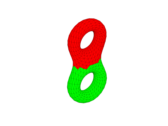
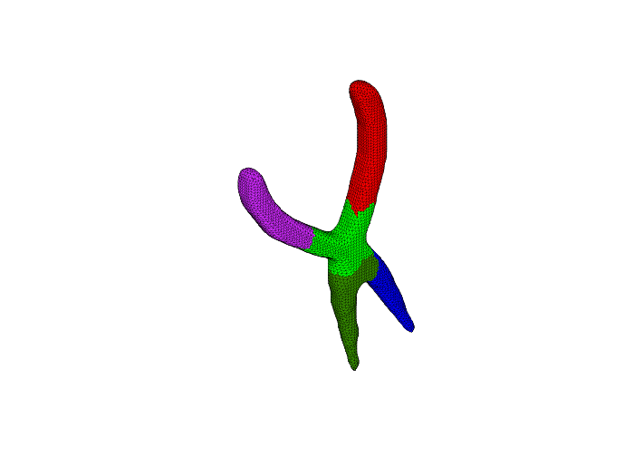
Figure 3: Left: segmentation with the angular distance of the cube model. The clusters are obtained computing $1\%$ of the $10800$ columns of $W$. Center: segmentation of the eight model with the geodesic distance obtained computing $2\%$ of the $1536$ columns of $W$. Right: pliers model segmentation with the sdf distance obtained computing $5\%$ of the $8970$ columns of $W$.

In our next examples we use a product metric to compute the distance between neighboring triangles. More precisely, if the faces $f_{i}$ and $f_{j}$ share an edge of the triangulation, then the product distance $d_{ij}$ between them is defined as $d_{ij}:=d_{ij}^{g}d_{ij}^{a}$, where $d_{ij}^{g}$, $d_{ij}^{a}$ are the geodesic and angular distances between $f_{i}$ and $f_{j}$ respectively. As usual, the distance between no adjacent faces is defined as the length of the shortest path in the dual graph. Figure 4 left shows the segmentation in $8$ clusters of the bunny model. This result was obtained computing the $10\%$ of the total number of columns of the affinity matrix $W$. Observe that the segmentation produced by the product distance distinguishes well not only the big ears but also the small tail. The hand model with $3000$ faces is more challenging. As we observe in Figure 4 right, there is some leakage in the clusters corresponding to the fingers, even when this leakage is substantially smaller than the one shown in the hand model in [26]. Moreover, the palm and the back of the hand belong to different clusters since the combined metric is not enough to capture all the volumetric information. These limitations could be overcome if we include in the definition of the combined metric a part-aware distance, such as the part-aware distance in [28].

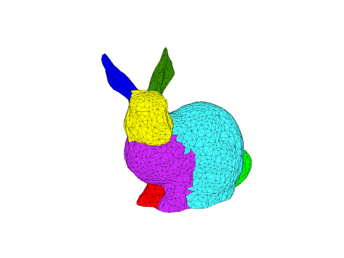
Figure 4: Two segmentations obtained with the metric defined as the product of geodesic and angular distances. Top: two views of the segmentation of the bunny model. The segmentation was computed using $10\%$ of the $3860$ columns of the affinity matrix $W$. Bottom: two view of the segmentation of the hand model, segmentation obtained computing $1\%$ of the $3000$ columns of $W$ .

5.3 Mesh segmentation quantitative performance

In this section we study the behavior of our mesh segmentation algorithm FSS through several examples of the Princeton Segmentation Benchmark [6] for evaluation of 3D mesh segmentation algorithms. This benchmark comprises a data set with 380 surface meshes of 19 different object categories. It also provides a ground-truth corpus of 4300 human segmentation.

In the next examples we observe that the algorithm proposed in this paper, based on the computation of few columns of the affinity matrix, produces segmentations which compare to the results obtained using the full affinity matrix. Recall that it doesn’t mean that the segmentation obtained with few columns of the affinity matrix $W$ is always good, but that it is as good as the one obtained computing all columns of $W$. In other words, if we select carefully which columns of $W$ are computed, then the quality of the results essentially depends on how good the selected metric reflects the features of the triangulation. In our experiments we compute the distance between triangles using several metrics: the geodesic distance, the angular distance, the product of them and the sdf distance [40].

Usually, the quantitative evaluation of a segmentation algorithm is done by comparing the automatic segmentation with one or more reference segmentations of the ground-truth corpus. In the literature one can find several metrics to evaluate quantitatively the similarity between two segmentations of a triangulated surface [3], [6]. In this section we employ two different non-parametric measures: the Jaccard index $JI$ [10] and the Rand index $RI$ [36]. The segmentation of a mesh with $n$ triangles may be described by a vector $s=(s_{1},...,s_{n})$, where $s_{j}$ is the index of the cluster to which the $j$-th triangle belongs. Given two segmentations $s_{a}$ and $s_{b}$ of the same mesh, we denote by $JI(s_{a},s_{b})$ and $RI(s_{a},s_{b})$ the similarity between them according to the Jaccard and Rand indexes respectively. For both indexes it holds: $0\leq JI(s_{a},s_{b})\leq 1$ and $0\leq RI(s_{a},s_{b})\leq 1$, where the value $1$ corresponds to the maximal similarity, i.e. $JI(s_{a},s_{b})=1$ or $RI(s_{a},s_{b})=1$ means that segmentations $s_{a}$ and $s_{b}$ are identical. In the experiments we compute Jaccard and Rand distances between $s_{a}$ and $s_{b}$ given by, $d_{J}(s_{a},s_{b}):=1-JI(s_{a},s_{b})$ and $d_{R}(s_{a},s_{b}):=1-RI(s_{a},s_{b})$.

In Figure 5 we show the results obtained for three models of the Princeton Segmentation Benchmark: the sunglasses (model 42), the octopus (model 121) and the bird ( model 243). For all models, Rand and Jaccard distances are computed comparing the automatic segmentation (left column) with and the ground truth segmentation (right column). Table 1 below shows the values of Rand and Jaccard distances as well as the percent of columns of the affinity matrix used to obtain the automatic segmentation and the metric employed for computing the distance between triangles. In these examples a low percent of columns provides good segmentations.

Example	distance	$\%$	$d_{R}$	$d_{J}$
glasses	geodesic	$2\%$	$0.062$	$0.161$
octopus	angular	$1\%$	$0.052$	$0.100$
bird	sdf	$1\%$	$0.048$	$0.295$

Table 1: Rand and Jaccard distances ( $d_{R}$ and $d_{J}$, respectively) between the automatic segmentation and the ground truth segmentation.

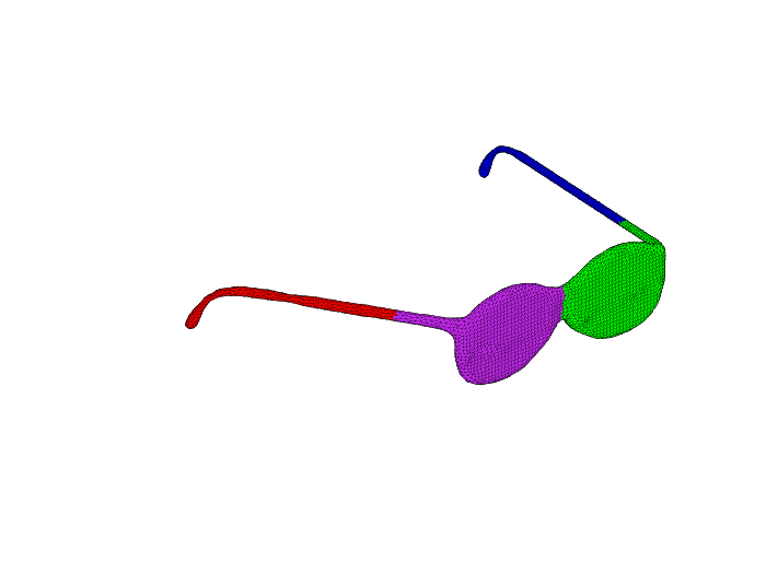
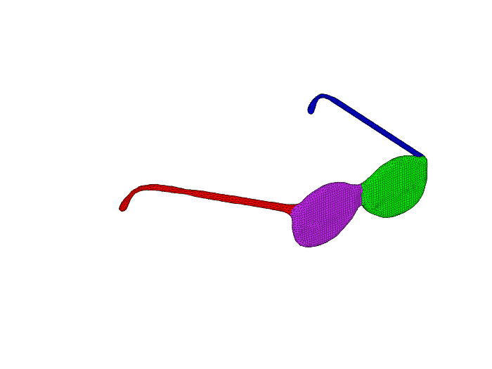
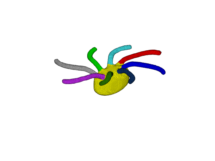
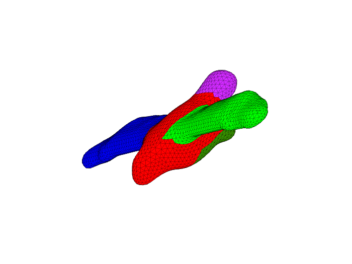
Figure 5: Left column: segmentations obtained computing few columns of the matrix $W$, right column: ground truth segmentations. First row: segmentation of the sunglasses based on geodesic distance and obtained computing $2\%$ of the $8324$ columns of $W$. Second row: segmentation of the octopus based on the angular distance and obtained computing $1\%$ of the $11888$ columns of $W$. Third row: segmentation of the bird based on the sdf distance and obtained computing $1\%$ of the $6312$ columns of $W$.

In Figure 6 we illustrate that the quality of the automatic segmentation with few columns of $W$ strongly depends on the capability of the selected metric to capture the features of the mesh. In this example we show that even if we compute the whole affinity matrix $W$, the resulting automatic segmentation is far a way from the ground truth segmentation, as it is shown by the values of $d_{R}$ and $d_{J}$ between these segmentations ($d_{R}=0.415$, $d_{J}=0.742$). On the other hand, the automatic segmentations obtained computing $0.5\%$ and $100\%$ of the columns of $W$ are very similar, since the values of $d_{R}$ and $d_{J}$ between them are small ($d_{R}=0.010$ and $d_{J}=0.064$). Hence, the segmentation with few columns is also not good in comparison with the ground truth segmentation. Finally, in this example we also observe that the body of fish is subdivided in clusters with similar areas. As other authors pointed out [6], this behavior is typical of segmentations based on k-means algorithm.

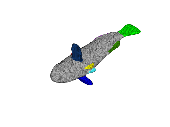
Figure 6: Three segmentations of a fish (model 225 of the Princeton Segmentation Benchmark). Left and center: segmentations based on the geodesic distance obtained using the $0.5\%$ and the $100\%$ of the $12148$ faces. Rand and Jaccard distances between them are $d_{R}=0.010$ and $d_{J}=0.064$ respectively. Right: ground truth segmentation. Rand and Jaccard distances between the segmentation obtained computing all the columns of $W$ and the ground truth segmentation are $d_{R}=0.415$, $d_{J}=0.742$.

5.4 Quality of segmentations: a different way of measuring.

In the experiments of this section we use a different approach to measure the quality of the segmentation. Instead of comparing the automatic segmentation, obtained computing $k$ columns of the affinity matrix, with the ground-truth of the corpus, we compare it with the segmentation obtained using all columns of the affinity matrix. In our opinion, this comparison is fairer, since the simple metrics (geodesic, angular and sdf distances) that we have used to compute the distance and affinity matrices are not always enough to produce good segmentations. Hence, the comparison of the automatic segmentations with ground-truth corpus segmentations does not help in the sense of proving that the results with few well selected columns of the affinity matrix are of quality quite similar to the results obtained computing all affinity matrix.

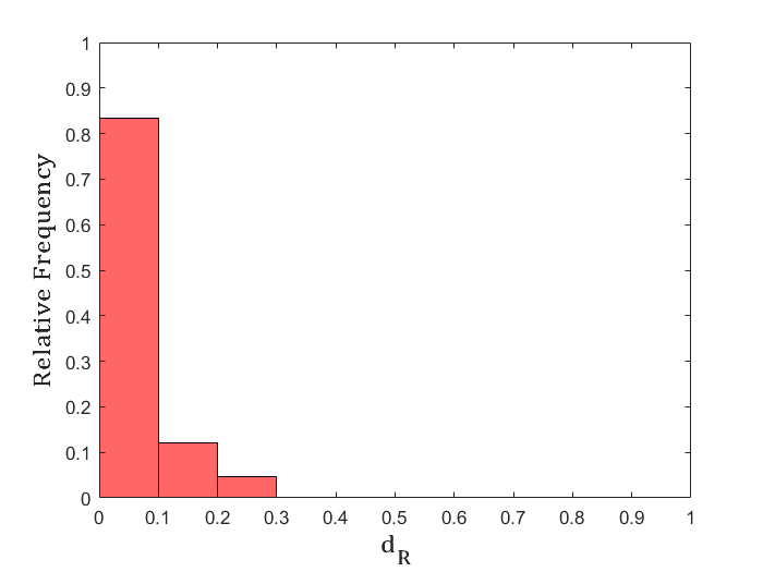
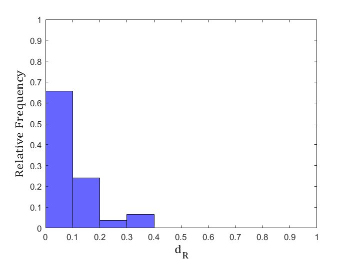
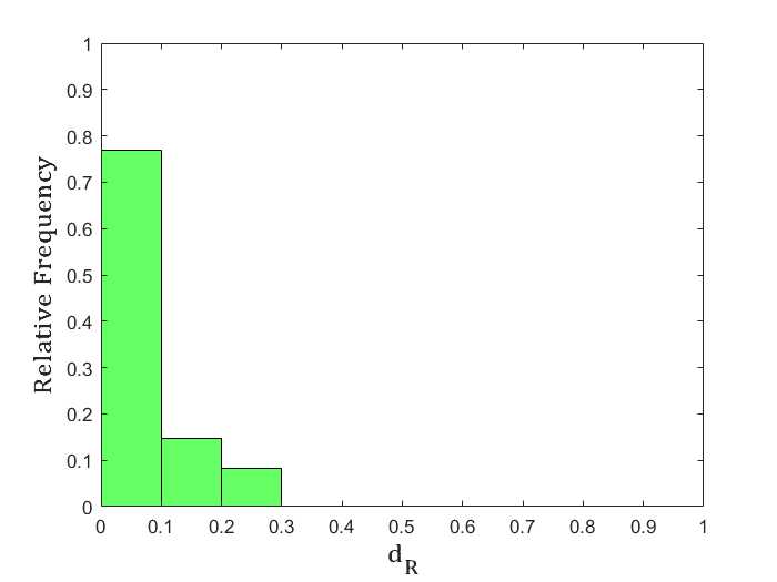
Figure 7: Relative frequency histograms of the Rand distance values, $d_{R}$, between the segmentations obtained with the whole matrix $W$ and the segmentation obtained with the same metric for $k$ columns of $W$, with $k=0.5\%,1\%,2\%,5\%,10\%,25\%$. From left to right: geodesic,angular and sdf metric.

Applying our segmentation method, $18$ meshes of the Princeton Segmentation Benchmark [6] are segmented using $k$ columns of the affinity matrix $W$, where $k=0.5\%,1\%,2\%,5\%,\%10$ and $\%25$ of the total number $n$ of faces. The Rand distance $d_{R}$ between the segmentations obtained for $k$ columns and the segmentation obtained with the same distance for the whole matrix $W$ is computed. Three different metrics are considered, the geodesic, the angular and the sdf metrics. For each of these metrics, in Figure 7 it is shown the histogram of relative frequency of the Rand distance values between the segmentations obtained for $k$ columns and the segmentation obtained with the same metric for the whole matrix $W$. This experiment shows that with high probability, the segmentations with small number of columns $k$ are very close to the corresponding segmentation obtained for the whole matrix $W$.

5.5 The $\beta$ curve

The graph of $\beta_{k}$ (17) as function of $k$ has a “L”-shape, similar to the singular values curve, which decreases very fast for small values of $k$, see Figure 2. It suggests that $\beta$ curve could be used to propose an lower bound for the size $k$ of the sample that furnishes a projection $H^{k}$ providing a good approximation to $W$. In the first row of Figure 8 it is shown a section of the $\beta$ curve $(k,\frac{\beta_{k}}{\beta_{1}}),\;1\leq k\leq n$ for three models of the Princeton Segmentation Benchmark (hand, bearing, octopus), considering different distances (geodesic, angular, sdf, respectively). Observe that these curves decrease very fast for small values of $k$ and tend slowly to 0 when $k$ goes to $n$.

For several values of $k$, Table 2 shows the Rand and Jaccard distances between the automatic segmentation $s_{k}$ and the ground truth segmentation of the Princeton Segmentation Benchmark. The smallest number of columns for which the slope of the $\beta$ curve may be considered as very small are marked with $*$. Observe that for any fixed model and all considered values of $k$, the values of the Rand and Jaccard distances between the automatic segmentation and the ground truth segmentation are very similar. In the second row of Figure 8 the segmentations corresponding to $k^{*}$ are shown.

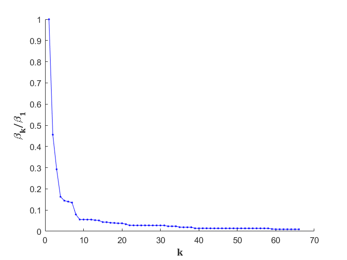
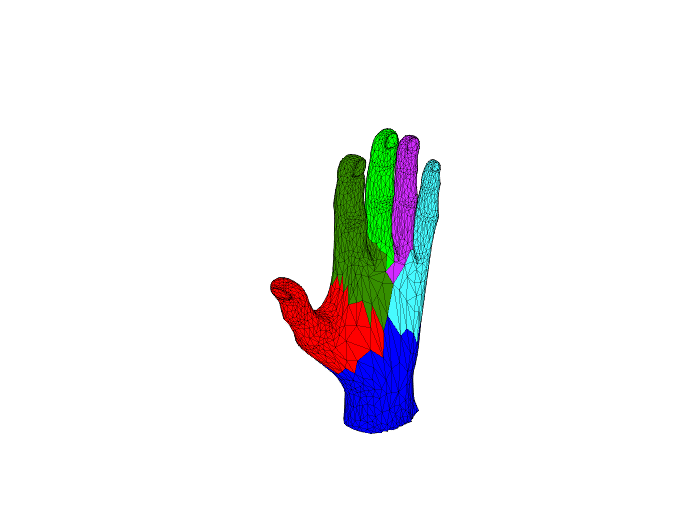
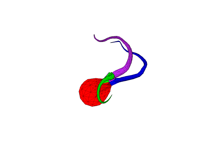
Figure 8: First row: normalized curve $\beta_{k}/\beta_{1}$ curve. Second row: segmentation of the models with $k^{*}$ columns of $W$.

Example	distance	$k$	$d_{R}$	$d_{J}$
hand	geodesic	$49^{*}$	$0.124$	$0.303$
$4979$ faces		$497$	$0.124$	$0.303$
		$1243$	$0.123$	$0.302$
bearing	angular	$16^{*}$	$0.033$	$0.452$
$3322$ faces		$66$	$0.033$	$0.452$
		$166$	$0.028$	$0.452$
octopus	sdf	$53^{*}$	$0.043$	$0.105$
$2682$ faces		$187$	$0.040$	$0.100$
		$321$	$0.040$	$0.099$

Table 2: Rand and Jaccard distances ( $d_{R}$ and $d_{J}$ respectively) between the proposed automatic segmentation and the ground truth segmentation. The automatic segmentation was obtained using the metric indicated in the second column and computing the number of columns of the affinity matrix indicated in the third column.

5.6 Comparing our method with the spectral approach

Since the method FSS proposed in this paper has some points of contact with the one introduced in [26] and improved in [25], in this section we compare the segmentations obtained with both approaches. The algorithm introduced in [25] applies Nyström’s method to approximate the spectral embeddings of faces of the triangulation. To avoid the expensive computation of the normalized matrix $Q=M^{-1/2}WM^{-1/2}$ and its largest eigenvectors, Nyström’s method computes approximately the largest eigenvectors of $Q$, from a small sample of its rows (or columns) and the solution of a small scale eigenvalue problem (see section 2.2). The final step consists in applying k-means to the rows of $Q$. The selection of the sample has a strong influence on the accuracy of the approximated eigenvectors.

No comments on the recommended relationship among the size of the sample and the number of eigenvectors are included in [25]. In the numerical experiments reported here, the same sample of max-min farthest faces is used to select the columns of $W$ to be computed by our method FSS and also for the Nyström approximation of the largest eigenvectors of $W$. Further, in the results obtained with the spectral method, we set the number of eigenvectors equal to the number of clusters. Moreover, as suggested in [11], the Nyström approximated eigenvectors of $Q$ are orthogonalized before applying k-means clustering.

Figure 9 shows the segmentation based on the sdf distance of several models, using the spectral method with Nyström approximation and our method FSS. Both methods compute the same percent of columns of $W$ corresponding to the farthest triangles. Table 3 shows the values of Rand and Jaccard distances between the corresponding segmentations. In general we observe that even when the segmentation are different, the quality of them is similar. The Rand distance between segmentations are very small in all cases, but Jaccard distances are larger reflecting better the visual differences.

Figure 9: First row: Spectral segmentations with Nyström approximation, the number of eigenvectors is equal to the number of clusters. Second row: segmentations obtained with our method FSS. The sample of columns of the affinity matrix is the same in both approaches: $0.5\%$ for the hand, $25\%$ for dog and $5\%$ for fawn.

Example	$\%$	$d_{R}$	$d_{J}$
hand	$0.5\%$	$0.054$	$0.229$
dog	$25\%$	$0.082$	$0.406$
fawn	$5\%$	$0.084$	$0.397$

Table 3: Rand and Jaccard distances between our segmentation and the segmentation produced by the spectral approach using Nyström approximation. The sample of columns of $W$ is the same for both methods. The second column of the table indicates the size of the sample which is the indicated $\%$ of the total number of triangles.

In our last example we show an unexpected artefact that we have observed. Sometimes the spectral segmentation obtained using Nyström approximation produces clusters which are non connected. This undesirable effect is eliminated when we increase the size of the sample of columns of the affinity matrix $W$. In contrast, our segmentation approach using the same sample of columns of $W$ always produces connected clusters (recall lemma 1). In Figure 10 left we show the spectral segmentation of the woman model obtained with the normalized matrix $Q$. Center and right images of this figure show the spectral segmentation with Nyström approximation and with the method proposed in this paper, both using $5\%$ of columns of $W$ corresponding to the farthest triangles in the sdf distance. The described artefact becomes evident in the spectral segmentation with Nystrom approximation.

Figure 10: Left: spectral segmentation computing all columns of the affinity matrix, center: spectral segmentation with Nyström approximation computing $5\%$ of columns of the affinity matrix $W$, right: our segmentation based in the same sample of columns of $W$.

6 Conclusions and future work

We have proposed a segmentation method for triangulated surfaces that only depends on a metric to quantify the distance between triangles and on the selection of a sample of few triangles. The proposed method computes the weighted dual graph of the triangulation with weights equal to the distance between neighboring triangles. The $k$ farthest triangles in the chosen metric are used to compute a rectangular affinity matrix $W^{k}$ of order $n\times k$, where the number $k$ of columns is much smaller than the total number of triangles $n$. Rows of $W^{k}$ encode the similarity between all triangles and the $k$ triangles of the sample. Thus, clustering the rows of $W^{k}$ happens to be consistent with the results of clustering the rows of the whole matrix $W$ and no artefact appears. Hence, a valid strategy to solve the segmentation problem consists in clustering the rows of $W^{k}$ by using for instance the k-means algorithm.

From the theoretical point of view the problem of reducing the dimensionality for clustering is strongly connected with the low rank approximation of the matrix containing the data to be clustered, which in our context is the affinity matrix $W$. In this sense, we have proved that for any sample $\mathcal{X}$ of $k$ indexes, the rank $k$ approximation of $W$ obtained projecting it on the space generated by the columns of $W$ with indexes in $\mathcal{X}$, coincides with the rank $k$ approximation obtained projecting $W$ on the space generated by its approximated eigenvectors, computed by Nyström’s method with the same sample of columns of $W$. Moreover, it is shown that if the columns of $W^{k}$ correspond to the $k$ farthest triangles in the selected metric, then the proximity relationship among the rows of $W^{k}$ tends to faithfully reflect the proximity among the corresponding rows of $W$.

In practice, our experiments have confirmed that this occurs even for relatively small $k$, resulting in a low computational cost method. Multiple experiments with a large variety of 3D triangular meshes were performed and they have shown that the segmentations obtained computing less than the $10\%$ of columns of the affinity matrix $W$ are as good as those obtained from clustering the rows of the full matrix $W$. We have also observed that the quality of the results, objectively measured in terms of Rand and Jaccard distances between the automatic and the ground truth segmentations, depends strongly on the capability of the selected metric of capturing the geometrical features of the mesh. Our experiments with geodesic, angular and sdf distances show that none is enough to produce good segmentations in all cases. A combination of two o more metrics usually leads to better results.

Compared to other segmentation methods considered in the literature, the segmentation method proposed in this paper has several advantages. First, it does not depend on parameters that must be tuned by hand. Second, it very is flexible since it can handle any metric to define the distance between triangles. Finally, it is very cheap, with a computational cost of $O(nm)$, where $m$ is the cost of computing the distance between two faces of the triangulation. In this sense, the proposed method is cheaper than spectral segmentation methods, which in the best case ( when Nyström approximation is used ) compute additionally the eigenvectors of an order $k$ matrix, with an extra cost of $O((n-k)k^{2})+O(k^{3})$ operations.

In the present work, we intentionally focus on simple single segmentation fields on $3D$ meshes and the clustering is obtained applying a well know clustering algorithm, k-means++, in order to achieve straightforwardly a fair comparison of our segmentation method with the spectral method. Nevertheless, our farthest point based segmentation FSS method may be extended to more complicated scenarios, where several attributes are combined in a single segmentation field, such as in [28], [43] or where several multi-view clustering methods have been proposed to integrate without supervision multiple information from the data, [16], [5]. Therefore, in the future, we plan to investigate the advantages of replacing Nyström’s method with ours, for instance, compare with [44], [9], in order to make the proposed algorithms more efficient in terms of computational and memory complexity as well as to obtain segmentations without artifacts, such as nonconnected clusters. Finally, it is worth mentioning that the basic ideas of our segmentation method - to compute only few columns of the affinity matrix and to apply a clustering algorithm to the rows of this submatrix - could be straightforwardly used in other segmentation or clustering problems, for instance in segmentation of digital images [30].

References

References

- AV [07] Arthur, D., Vassilvitskii, S., k-means++: The Advantages of Careful Seeding, SODA ’07: Proceedings of the Eighteenth Annual ACM-SIAM Symp.on Discrete Alg., 2007, 1027–1035.
- BH [03] Brand, M., Huang, K., A unifying theorem for spectral embedding and clustering, in Proc. of Int. Conf. on AI and Stat., Florida, 2003.
- BH [03] Benhabiles H., Vandeborre, J.P., Lavoué, G., Daoudi, M., A comparative study of existing metrics for 3D-mesh segmentation evaluation, The Visual Computer 26, 1451–1466, 2010.
- BZMD [15] Boutsidis, C., Zouzias, A., Mahoney, M. W., Drineas, P., Randomized dimensionality reduction for k-means clustering, IEEE Trans. on Inf. Theory, 61(2), 1045–1062, 2015.
- CNH [13] Cai, X., Nie, F., Huang, H., Multi-view k-means clustering on big data, in Proceedings of the Twenty-Third international joint conference on Artificial Intelligence, AAAI Press, 2598–2604, 2013.
- CGF [09] Chen, X., Golovinskiy, A., Funkhouser, T., A benchmark for 3D mesh segmentation, ACM Transactions on Graphics (SIGGRAPH) 28 (3), 2009.
- EK [03] Elad A., Kimmel, R., On bending invariant signatures for surfaces, IEEE Trans. Pat. Ana. Mach. Int. 25 (10), 1285–1295, 2003.
- EY [36] Eckart C., Young, G., The approximation of one matrix by another of lower rank, Psychometrika 1, 211–218, 1936.
- EFKK [14] Elgohary, A., Farahat, A.K., Kamel, M. S., Karray, F., Embed and conquer: Scalable embeddings for kernel k-means on MapReduce, in The SIAM International Conference on Data Mining (SDM), 2014.
- FM [83] Fowlkes, E.B., Mallows, C.L., A method for comparing two hierarchical clusterings, Journal of the American statistical association 78 (383), 553–569. 1983.
- FBCM [04] Fowlkes C., Belongie S., Chung, F., Malik, J., Spectral grouping using the Nyström method, IEEE Trans. Pat. Ana. Mach. Int. 26 (2), 214–225, 2004.
- GSCO [07] Gal R., Shamir A.,Cohen-Or, D., Pose-oblivious shape signature, IEEE Trans. Vis. and Comp. Graphics 13 (2), 261–271, 2007.
- dGGV [08] de Goes F., Goldenstein, S., Velho, L., A hierarchical segmentation of articulated bodies, Computer Graphics Forum (Symposium on Geometry Processing), 27(5), 1349–1356, 2008.
- Got [03] Gotsman, C., On graph partitioning, spectral analysis, and digital mesh processing, in Proc. IEEE Int. Conf. on Shape Modeling and Applications, 165–171, 2003.
- HIW [15] Holodnak, J.T., Ipsen, I.C.F., Wentworth, T., Conditioning of Leverage Scores and Computation by QR Decomposition , SIAM J. Matrix Anal. Appl., 36(3), 1143–1163, 2015.
- HCC [12] Huang, H-C., Chuang,Y-Y., Chen, C-S., Affinity aggregation for spectral clustering, in IEEE Conference on Computer Vision and Pattern Recognition (CVPR), 773–780, 2012
- JZK [07] Jain, V., Zhang, H., van Kaik, O., Nonrigid spectral correspondence of triangle meshes, Int. J.on Shape Modeling 13 (1), 101–124, 2007.
- Jol [72] Jolliffe, I., Discarding variables in a principal component analysis: Artificial data, Applied Statistics, 21 (2), 160–173, 1972.
- KT [03] Katz, S., Tal, A., Hierarchical Mesh Decomposition Using Fuzzy Clustering and Cuts, ACM Transactions on Graphics, 22 (3), 954–961, 2003.
- KLT [05] Katz, S., Leifman, G., Tal, A., Mesh segmentation using feature point and core extraction, The Visual Computer (Special Issue of Pacific Graphics) 21, 8-10 , 649–658, 2005.
- KSW [04] Kleinberg, J., Slivkins, A., Wexler, T., Triangulation and embedding using small sets of beacons, in 45th Annual IEEE Symposium, FOCS, 444–453, 2004.
- KMA [12] Kumar, S., Mohri, M., Talwalkar, A., Sampling Techniques for the Nyström Method, J. Mach. Learn. Res. 13, 981–1006, 2012.
- LLSCS [05] Lee, Y., Lee, S., Shamir, A., Cohen-Or, D., Seidel, H. P., Mesh scissoring with minima rule and part salience, Comput. Aided Geom. Des. 22 (5), 444–465, 2005.
- Lloyd [82] Lloyd, S., Least squares quantization in PCM, IEEE Transactions on Information Theory, 28(2):129–137, 1982.
- LJZ [06] Liu, R., Jain, V., Zhang, H., Subsampling for efficient spectral mesh processing, in Proc. of Computer Graphics International, 172–184, 2006.
- LZ [04] Liu, R., Zhang, H., Segmentation of 3D Meshes through Spectral Clustering, in Proc. Pacific Graphics, 298–305, 2004.
- LZ [07] Liu, R., Zhang, H., Mesh Segmentation via Spectral Embedding and Contour Analysis, EUROGRAPHICS 2007, Ed D. Cohen-Or and P. Slava, 26, 2007.
- LZSC [09] Liu, R., Zhang, H., Shamir, A., Cohen-Or, D., A Part-aware Surface Metric for Shape Analysis, EUROGRAPHICS 2009, Ed. P. Dutré and M. Stamminger, 28 (2), 397–406, 2009.
- Mah [11] Mahoney, M., Randomized algorithms for matrices and data, Foundations and Trends in Machine Learning, NOW Publishers 3 (2), 2011.
- MiCh [16] Miao, J., Chen, D., A Spectral Clustering Image Segmentation Algorithm Based on Nyström Approximation, International Conference on Computational Modeling, Simulation and Applied Mathematics (CMSAM 2016), ISBN: 978-1-60595-385-4, 2016.
- MTAD [08] Mullen, P., Tong, Y., Alliez, P., Desbrun, M., Spectral conformal parameterization, Computer Graphics Forum (Symposium on Geometry Processing) 27 (5), 1487–1494, 2008.
- NgW [02] Ng, A., Jordan, M., Weiss, Y., On spectral clustering: Analysis and an algorithm, Advances in neural information processing systems, 2:849–856, 2002.
- PKA [03] Page, D. L., Koschan, A., Abidi, M. A., Perception based 3d triangle mesh segmentation using fast marching watersheds, in Proc. IEEE Conf. on Comp. Vis. and Pat. Rec., 27–32 , 2003.
- PBCG [09] Potamias, M., Bonchi, F., Castillo, C., Gionis, A., Fast shortest path estimation in large networks, Proceedings CIKM’09, 866–876, 2009.
- PBCG [09] Potamias, M., Bonchi, F., Castillo, C., Gionis, A., Fast shortest path estimation in large networks, Proceedings CIKM’09, 866–876, 2009.
- Rand [71] Rand, W., Objective criteria for the evaluation of clustering methods, Journal of the American Statistical Association 66, 846–850, 1971.
- RBGPS [09] Reuter, M., Biasotti, S., Giorgi, D., Patane, G., Spagnuolo, M., Discrete Laplace-Beltrami Operators for Shape Analysis and Segmentation, SMI’09, Computers and Graphics 33 (3), 381–390, 2009.
- Sha [08] Shamir, A., A survey on mesh segmentation techniques, Computer Graphics Forum 27 (6), 1539–1556, 2008.
- ST [04] da Silva, V., Tenenbaum, B., Sparse Multidimensional Scaling using Landmark Points, Tech. Rep., Stanford University, June 2004.
- SSCO [08] Shapira, L., Shamir, A., Cohen-Or, D., Consistent mesh partitioning and skeletonization using the shape diameter function, Visual Computer 24 (4), 249–259, 2008.
- SM [97] Shi, J., Malik, J., Normalized Cuts and Image Segmentation, Proceedings of IEEE Conference on Computer Vision and Pattern Recognition, 731–737, 1997.
- vL [06] von Luxburg, U., A Tutorial on Spectral Clustering, Tech. Rep. TR-149, Max Plank Institute for Biological Cybernetics, August 2006.
- WTKL [14] Wanga, H., Lu, T., Au, O., Tai, C-L., Spectral 3D Mesh Segmentation with a Novel Single Segmentation Field, Graphical Models, 76 (5), 440–456, 2014.
- YLMJZ [12] Yang, T., Li, Y-F., Mahdavi, M., Jin, R., Zhou, Z-H., Nyström method vs random fourier features: A theoretical and empirical comparison, in Advances in neural information processing systems, 476–484, 2012.
- ZL [05] Zhang, H., Liu, R., Mesh segmentation via recursive and visually salient spectral cuts, in Proc. of Vision, Modeling, and Visualization, 2005.
- ZVKD [10] Zhang, H., van Kaick, O., Dyer, R., Spectral Mesh Processing, Computer Graphics Forum 29 (6), 1865–1894, 2010.