Keywords: Nonlinear Solid Mechanics $\cdot$ Adaptive Mesh Refinement $\cdot$ Unfitted finite elements $\cdot$ Embedded boundary methods $\cdot$ Tree-based meshes $\cdot$ Parallel computing.

1. Introduction

Meeting the Computer Aided Engineering (CAE) demands of many industrially-relevant settings nowadays involves the solution of ever increasing computationally intensive problems. Problems posed on complex geometries, which may evolve over time, are routinely encountered. To further increase the challenge, the physical phenomena subject to analysis typically exhibit localized features, so that the use of adaptive meshing techniques becomes paramount towards achieving an optimal accuracy versus computational efficiency balance.

A paradigmatic application problem is Additive Manufacturing (AM). AM enables complex designs with highly desirable properties largely unachievable by conventional manufacturing processes. For instance, AM is well-suited for producing parts with complex mesoscale lattice structures. The shape and interconnection pattern of unit cells hold a large influence over the mechanical properties of such structures (e.g. stress-strain response) [1]. The design of this microstructure to obtain the desired mechanical properties can be made using topology optimization [2]. Another example is the thermo-mechanical simulation of metal AM processes, which requires that one designs a virtual mechanism that generates the growing geometry of the part being manufactured following the real scanning path of the machine. Besides, very fine resolution close to the heated moving head is required in order to accurately capture the high thermal gradients inherent to AM [3], which induce distortion and residual stresses.

All this complexity limits the applicability of CAE tools traditionally used in industrial settings. These tools are almost invariably based on FEs on conforming, unstructured, body-fitted meshes. Their generation for complex geometries is a challenging task, and in many cases requires human intervention. This becomes impractical when considering an external optimization loop or growing-in-time geometries, as these would require the generation of a mesh at every iteration of the process. To make things worse, parallel unstructured mesh generation and partitioning (e.g. via graph partitioning) scales poorly on parallel computers.

The approach that we advocate to effectively manage all this complexity relies on the so-called embedded (a.k.a. unfitted) FE methods. The differential equation at hand is discretized by embedding the computational domain in an easy-to-generate background mesh that does not necessarily conform to its geometrical boundary, thus drastically reducing the geometrical constraints imposed on the meshes to be used for discretization. The geometry is still provided explicitly in terms of a boundary representation (e.g. a STereoLithography (STL) mesh) or implicitly via the zero isosurface of a level-set function. Essentially, by intersecting the surface and background meshes, one generates a sub-mesh of each cut cell that conforms to the boundary, thus generating a discretization of the domain (such discretization is only used for integration purposes, though).

Embedded methods can be used with a variety of background mesh types. The approach herein particularly leverages octree-based meshes but the FE schemes can readily be used for simplicial meshes. Octrees are recursively structured hexahedral grids which have multi-resolution capabilities. This is achieved by means of a recursive approach in which a mesh with a very coarse resolution (in the limit, a single cube that embeds the entire domain) is recursively refined step-by-step, until all mesh cells fulfill suitably-defined (geometrical and/or numerical) error criteria. As the terminal cells in the resulting tree-like hierarchy might be at different refinement levels, the resulting meshes are non-conforming, i.e. they have the so-called hanging Vertices, Edges, and Faces at the interface of neighboring cells with different refinement levels. Such relaxation of conformity becomes crucial for high parallel scalability. Besides, octree-based meshes, endowed with Space-Filling curves, enable the development of petascale-capable AMR FE simulation pipelines, while efficiently addressing load unbalance caused by localization via dynamic load-balancing in the course of the simulation [4, 5].

On the downside, cut cells pose serious drawbacks that have reduced the applicability of embedded methods. The most concerning is that they lead to ill-conditioned discretizations in general. Cut cells with a small portion in the interior have a dramatic impact on the condition number of the linear system. Recently, different approaches have been considered to address this issue. A family of approaches add stabilization terms to the discrete problem, using some kind of artificial viscosity method to make the problem well-posed; see, e.g. the CutFEM method [6] or the Finite Cell Method (FCM) [7]. More recently, the Aggregated Finite Element Method (AgFEM) method was developed in [8, 9]. This method builds a kind of $\mathcal{C}^{0}$ Lagrangian FE spaces that can be defined on general agglomerated meshes with arbitrary shapes. Numerical stability is achieved by eliminating the DOFs laying at the exterior of the domain via suitably-defined linear algebraic constraints (in terms of a discrete extension operator), letting one stick to a Galerkin discretization. Besides, AgFEM can be remarkably combined with octree-based $h$-adaptive background meshes, while being very amenable to parallelization on large-scale parallel machines [10, 11]. The $h$-AgFEM method, developed in [10, 12], combines AgFEM with parallel AMR implemented on distributed-memory platforms, and paves the road to functional and geometrical error-driven dynamic mesh adaptation with the FE method in large-scale, industrially-relevant scenarios.

A common requirement in solid mechanics is the resolution of localized phenomena as, e.g. in strain localization and fracture problems. To be able to efficiently tackle these problems one has to use error estimators aiming at detecting the cells where the localized phenomena occurs (see, e.g. [13, 14]). Besides, parallel AMR and dynamic load-balancing becomes necessary to efficiently address mesh densification on localized areas. In [15], these techniques are used in order to address problems in contact mechanics with elasto-plastic solids on parallel distributed-memory computers, while in [16], a goal-oriented error estimator is developed for elasto-plasticity problems. The formulations presented in these papers are tailored to body-fitted meshes, though. On the other hand, unfitted formulations available in the literature are mainly restricted to linear or nonlinear elastic materials using non-adaptive meshes and serial implementations. An immersed FE method for interface problems was presented in [17] and [18], using signed distance functions to detect the relative position of the cell with respect to the surface describing the solid. The final geometry is then obtained by using Constructive Solid Geometry (CSG). A consistent extension of the FCM to handle structural mechanics problems was proposed in [19]. The method is applied to 2D and 3D elastic problems reproducing complex geometries imported via Computer Aided Design (CAD) and image-based geometric models. A similar approach is followed in [20] to reproduce 3D physical domains taken from human bone biopsies. The Cut Cell Method (CCM) method was also extended to solve linear elasticity problems in [21]. In contrast to previous works, the authors focus their attention on the usage of parametric representations to capture the domain boundary in complex geometries. They also extend this methodology to interface problems, in order to study the behavior of linear elastic composite materials, considering the embedding of thin elastic structures such as membranes and plates.

To the best of our knowledge, and despite of this active scientific progress in embedded modeling, very little effort has been devoted to the design of $h$-adaptive embedded modeling methods for large-scale problems in nonlinear solid mechanics. To fill this gap, we study the suitability of the $h$-AgFEM method [10] on parallel scalable octree background meshes, recently developed for linear elliptic problems, to efficiently address large-scale nonlinear solid mechanics problems exhibiting localized features, posed over complex geometries. To this end, we bridge for the first time in the literature standard AMR on scalable octree (background) meshes and novel unfitted FE methods in nonlinear solid mechanics. In turns out that in the extension $h$-AgFEM method [10] to this kind of problems there are several aspects that require a somewhat specialized treatment. We restrict ourselves to problems involving nonlinear materials whose behavior depends on the strain history, i.e. the constitutive models explored are based on history variables. This sort of problems are used as a demonstrator, but we stress that the techniques presented can also be applied to, e.g. problems with geometric nonlinearities. In general, and even more importantly under the presence of AMR, such variables have to be tracked appropriately in the course of a load increment simulation. To this end, we advocate for considering constitutive model history variables as fields, rather than a mere data array with values on quadrature points for numerical integration. For such functional representation, we choose a cell-wise polynomial, discontinuous Lagrangian FE space, with the same definition of DOFs for interior and cut cells, i.e. nodal values positioned at the tensor-product of Gauss quadrature points. This approach reduces memory demands and greatly simplifies the transfer of these variables between meshes compared to the permanent storage of history values at all quadrature points of the sub-meshes of all cut cells used for the evaluation of integrals over the embedded domain. Apart from this, this work relies on the following two main ingredients to achieve its goals:

1. An algorithm for the solution of strongly nonlinear problems, which composes the Newton-Raphson method with a line-search strategy with cubic backtracking. We leverage the suite of nonlinear and linear solvers available in the PETSc software package [22] for implementing such algorithm.

2. An algorithm to perform load increment (usually referred to as pseudo time-stepping) in combination with AMR. This algorithm is used to produce a locally refined background mesh while deformation is localizing and includes parallel dynamic load-balancing at each step. Up to the authors’ knowledge, the current literature (see, e.g. [15, 16]) does not seem to pay a careful attention to this ingredient. Our experience reveals that a proper tuning of the parameters of this algorithm for each problem at hand can have a significant impact on the balance struck in practice among accuracy and computational cost.

The discussion on these building blocks in the article focuses on the aspects that require a somewhat specialized treatment in an embedded setting.

This work is structured as follows. In Sect. 2, we state the class of nonlinear solid mechanics problems considered in this work, namely the stress analysis of nonlinear elasto-plastic solids under small strains and displacements. In Sect. 3, we introduce and motivate the spaces of functions used for spatial FE discretization and handling of history variables, resp., and the projection operators used to transfer FE functions in these spaces among two consecutive hierarchically adapted octree-based meshes (resulting from the application of AMR). In Sect. 4, we present a description of the pseudo-time discretization and the corresponding linearization of the nonlinear problem. In Sect. 5, we describe the algorithm to bridge pseudo-time integration and AMR in an embedded setting. In Sect. 6, we present a comprehensive numerical study to validate the framework, including a set of standard validation benchmarks, and large-scale experiments involving complex geometries, aiming at studying the accuracy and parallel scalability of the framework. Finally, in Sect. 7 we present some conclusions.

2. Problem statement

In this section we present the class of nonlinear solid mechanics problems considered herein, which include those involving nonlinear elasto-plastic materials. Elasto-plasticity models can be used to solve a wide range of industrial problems. Because they are well-known, we provide a succinct description of them and refer the reader to, e.g. [23, 24], for further details. As usual, we use regular characters for scalar fields and bold characters for vector and tensor fields. The two main ingredients of the model, namely the equilibrium equations and the constitutive models, are presented in Sect. 2.1 and 2.2, resp.

2.1. Equilibrium equations

We consider both compressible and incompressible materials in this work. The former kind of materials can be accurately modeled using an irreducible formulation, whereas the latter requires a mixed displacement-pressure formulation in which the pressure $p$ is computed separately.

Let ${\Omega}\subset\mathbb{R}^{d}$ be an open bounded domain in which the problem is posed, and ${\Gamma}$ its boundary. If we denote as ${{\Gamma}_{\rm D}}$ and ${{\Gamma}_{\rm N}}$, with ${\Gamma}={{\Gamma}_{\rm D}}\cup{{\Gamma}_{\rm N}}$, the regions of the boundary in which we impose Dirichlet and Neumann boundary conditions, resp., the irreducible formulation consists in finding $\boldsymbol{u}:{\Omega}\rightarrow\mathbb{R}^{d}$, the displacement field, such that:

$$\nabla\cdot\boldsymbol{\sigma}+\boldsymbol{f} =\mathbf{0} \mathrm{in} {\Omega}$$ (1)

$$\boldsymbol{u} =\overline{\boldsymbol{u}} \mathrm{on} {{\Gamma}_{\rm D}}$$

$$\qquad\boldsymbol{\sigma}\cdot{\boldsymbol{n}} =\boldsymbol{t} \mathrm{on} {{\Gamma}_{\rm N}}\ ,$$

given $\boldsymbol{f}:{\Omega}\rightarrow\mathbb{R}^{d}$ the body force per unit volume, $\overline{\boldsymbol{u}}:{{\Gamma}_{\rm D}}\rightarrow\mathbb{R}^{d}$ the displacement prescribed on ${{\Gamma}_{\rm D}}$, and $\boldsymbol{t}:{{\Gamma}_{\rm N}}\rightarrow\mathbb{R}^{d}$ the traction per unit area prescribed on ${{\Gamma}_{\rm N}}$. The unit normal pointing outwards on the boundary ${{\Gamma}_{\rm N}}$ is denoted by ${\boldsymbol{n}}$. The stress tensor $\boldsymbol{\sigma}$ depends nonlinearly on $\boldsymbol{u}$ as described in Sect. 2.2.

Formulation (1) fails for incompressible materials. In the mixed (u/p) formulation the volumetric part of the stress tensor $\boldsymbol{\sigma}$ is an additional unknown and a new equation imposing mass conservation is considered. The stress tensor is decomposed as $\boldsymbol{\sigma}=p\textbf{I}+\textbf{s}$, where $p=\frac{1}{3}\mathbf{tr}(\boldsymbol{\sigma})$ and $\textbf{s}=\textbf{dev}(\boldsymbol{\sigma})$, denote its volumetric and deviatoric parts, resp. The problem can be stated as finding the displacement $\boldsymbol{u}:{\Omega}\rightarrow\mathbb{R}^{d}$, and the pressure $p:{\Omega}\rightarrow\mathbb{R}$ satisfying (1) together with $\kappa^{-1}p-\nabla\cdot\boldsymbol{u}=0$ in ${\Omega}$, where $\kappa$ is the bulk modulus.

2.2. Constitutive model

The constitutive model describes the relation between stresses and strains. In this work, we consider the J2 Von Mises isotropic elasto-plasticity model. In any case, the framework is applicable to other constitutive models, e.g. damage or coupled plasticity-damage models. As is well known, this constitutive model accurately describes the stress-strain response of a wide range of ductile materials, such as, metals and fiber-reinforced composites. In the context of nonlinear modeling, the relation between stresses and displacements can be written as

$$\boldsymbol{\sigma}=\boldsymbol{\sigma}(\boldsymbol{u},\boldsymbol{\mu}),$$ (2)

that is, $\boldsymbol{\sigma}$ is a tensor function defined in terms of constitutive parameters and the projection operator of trial stresses onto the admissible stress space [15, 25, 14] (usually implemented using the so-called return mapping algorithm proposed by Simo in [23]) and $\boldsymbol{\mu}$ denotes the set of history variables. These variables play the role of tracking the nonlinearity of the constitutive model. Particularly, in J2 plasticity, since the plastic strain is considered isochoric, i.e. the volumetric part of the plastic deformations is zero, so the total volumetric deformation $\varepsilon_{v}$ is directly the elastic volumetric deformation, $\nabla\cdot\boldsymbol{u}$. The pressure $p$ is either an unknown (in the mixed formulation) or a dependent variable computed as $p=\kappa\nabla\cdot\boldsymbol{u}$ (in the irreducible formulation). In the case of the mixed formulation $\boldsymbol{\sigma}$ also depends on the pressure $p$, that is, (2) becomes $\boldsymbol{\sigma}=\boldsymbol{\sigma}(\boldsymbol{u},p,\boldsymbol{\mu})$.

The model is particularized by introducing a yield function that defines the limit of the elastic behavior, based on a given measure. In the case of J2-like models, this measure corresponds to the second deviatoric invariant of stresses. Concerning the set of history variables, in the isotropic case, this set is restricted to only one variable $\boldsymbol{\mu}=\alpha$. In order to particularize the constitutive model, we consider the following yield function

$$\phi=\frac{1}{2}\sqrt{\textbf{s}:\textbf{s}}-\sqrt{\frac{2}{3}}(\sigma_{y}-q(\alpha)),$$ (3)

where $\sigma_{y}$ denotes the yield stress, and $q$ the stress-like thermodynamic force. The latter is expressed as a function of the historical variable $\alpha$ with an exponential saturation law as

$$q(\alpha)=-\theta H\alpha-(K_{inf}-K_{0})[1-\text{exp}(-\delta\alpha)],$$ (4)

where $\theta$ is the activation parameter to take into account the linear isotropic hardening, $H$ denotes the hardening modulus, and $K_{inf}$, $K_{0}$ and $\delta$ are material constants. Without loss of generality, we restrict ourselves to associative elasto-plasticity models, where the yield function $\phi$ is taken as plastic flow rule. In consequence, the evolution of the plastic strain tensor $\boldsymbol{\varepsilon^{p}}$, and the history variables will depend on the choice of the yield function, i.e. (3); see [23] for further details.

3. Spatial FE discretization

Unfitted FE methods pose problems to the numerical integration and lead to ill-conditioned systems [26, 6, 8]. To address these issues, different techniques have been proposed and our goal here is to extend them to solve nonlinear solid mechanics problems. Specifically, we propose the extension of the $h$-AgFEM in [10]. We combine the conforming aggregated FE spaces in [10] to represent the state variables (i.e. either the displacement field or the displacement and pressure fields, depending on the formulation at hand) and discontinuous aggregated FE spaces (see, e.g. [27]) to represent internal variables.

After some general aspects of the embedded boundary setup in Sect. 3.1, we review the construction in [10] in Sect. 3.2 and we present the discontinuous aggregated FE spaces we use to represent internal variables in Sect. 3.3. Finally, in Sect. 3.4 we describe how to use the tools provided by these spaces to define the transfer operators between meshes, which are required to project all variables involved in the problem after the mesh is adapted.

3.1. Embedded FE setup

Let us consider an artificial (or background) cuboid-like domain ${\Omega^{\text{art}}}$, in which the physical domain is embedded, i.e. ${\Omega}\subset{\Omega^{\text{art}}}$ (see Fig. 1a). We denote by $\mathcal{T}_{h}$ a mesh for ${\Omega^{\text{art}}}$. In particular, we consider the so-called forest-of-trees [5] background meshes as the choice for $\mathcal{T}_{h}$. In a nutshell, these meshes are built as follows. First, one builds a coarse conforming mesh $\mathcal{T}_{0}$ (i.e. a quadrilateral mesh in 2D or hexahedral mesh in 3D) of ${\Omega^{\text{art}}}$. Next, each element of this coarse mesh is the root of a tree-based mesh (quadtree or octree) that is generated as a result of a sequence of hierarchical refinement/coarsening steps. In our implementation we rely on forest-of-trees meshes generated using the p4est library [28], which provides parallel peta-scalable mesh manipulation operations.

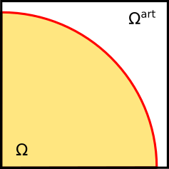
a

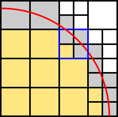
b

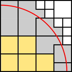
c

Figure 1. (A) Physical domain (unfitted boundary in red) embedded into the artificial domain ${\Omega^{\text{art}}}$, (B) tree-based background mesh $\mathcal{T}_{h}$ intersected with the physical domain in order to define the well-posed (in yellow), ill-posed (in gray) and exterior (in white) cells, (C) Aggregated mesh, well-posed cells (in yellow) and aggregates (in gray).

To describe the geometry of the physical domain ${\Omega}$, let us introduce now the immersed boundary setting on top of the artificial domain ${\Omega^{\text{art}}}$. The domain ${\Omega}$ (and its boundary $\partial{\Omega}$) can be represented by a level-set function or an oriented surface mesh (e.g. an STL mesh). The intersection of each cell $K\in\mathcal{T}_{h}$, with $\partial{\Omega}$ and ${\Omega}$ can be computed using a marching-cubes algorithm. We represent with $\mathcal{T}_{h}^{{\mathrm{act}}}$ (resp. $\mathcal{T}_{h}^{{\mathrm{cut}}}$) the set of active (resp., cut) cells in $\mathcal{T}_{h}$ that intersect ${\Omega}$ (resp., $\partial{\Omega}$); $\mathcal{T}_{h}^{{\mathrm{act}}}\setminus\mathcal{T}_{h}^{{\mathrm{cut}}}$ is the set of interior cells in ${\Omega}$. Numerical integration over cells $K\in\mathcal{T}_{h}^{{\mathrm{cut}}}$ can be carried out by computing a simplicial decomposition of $K\cap{\Omega}$, e.g. using a Delaunay triangulation. The triangulation which results from replacing cells $K\in\mathcal{T}_{h}^{{\mathrm{cut}}}$ by their decomposition is denoted by $\mathcal{T}_{h}^{{\mathrm{int}}}$. Other integration techniques that do not require simplicial sub-meshes, e.g. cubatures on general polytopes (see, e.g. [29]), can also be used.

These ingredients are enough to implement an embedded method but, as it was mentioned in Sect. 1, a solution for the small cut cell problem is required. The small cut cell problem appears when the ratio between the volume of the cell inside the domain and its total volume goes to zero. In this work, we consider as (potentially) ill-posed cells all cut cells and well-posed cells the interior cells; see Fig. 1b. A cell aggregation map is constructed to solve the small cut cell problem that can potentially appear in ill-posed cells; it is used to eliminate problematic DOFs, as it will be described in Sect. 3.2.2. This map assigns an interior (well-posed) cell to any cut (ill-posed) cell, located at the boundary of the physical domain. In order to define this map, cell aggregates are generated using the Algorithm 2.2 in [11]. Each aggregate is a connected set, composed of several ill-posed cells and only one well-posed root cell $T$ and they form another partition $\mathcal{T}_{h}^{\mathrm{ag}}$ (a so-called agglomerated mesh) of the domain ${\Omega^{\text{art}}}$; see Fig. 1c.

3.2. State variables discretization (via continuous Lagrangian FE spaces)

In this section we overview two possible choices of FE spaces for the discretization of the state variables. As required by the Galerkin FE discretization of the problem at hand, these spaces are $H^{1}$-conforming. We use them for the approximation of (each component of) the displacement field (and for the pressure field in the Taylor-Hood stable mixed approximation).

3.2.1. Standard (ill-posed) continuous Lagrangian FE spaces

Standard continuous Lagrangian FE spaces can be defined as:

$${\mathcal{V}}_{h}^{{\mathrm{std}}}(\mathcal{T}_{h}^{{\mathrm{act}}})\doteq\{v\in{\mathcal{C}^{0}}({\Omega})\,:\,v|_{T}\in{\mathcal{V}}_{k}(T)\text{ for any }T\in\mathcal{T}_{h}^{{\mathrm{act}}}\},$$ (5)

where ${\mathcal{V}}_{k}(T)$ stands for the space of functions defined on $T\in\mathcal{T}_{h}^{{\mathrm{act}}}$. Here, we consider ${\mathcal{V}}_{k}(T)\doteq{\mathcal{Q}}_{k}(T)$, the tensor product space of order $k$ univariate polynomials. Besides, we assume that all cells in $\mathcal{T}_{h}^{{\mathrm{act}}}$ have local spaces ${\mathcal{V}}(T)$ of the same order $k$.

When using a conforming mesh, the inter-cell continuity required by the definition of ${\mathcal{V}}_{h}^{{\mathrm{std}}}(\mathcal{T}_{h}^{{\mathrm{act}}})$, is implemented by using the nodal Lagrangian basis for ${\mathcal{Q}}_{k}(T)$ (the DOFs being the corresponding nodal values) and a local-to-global DOF map. However, in general, a tree-based background mesh $\mathcal{T}_{h}$ is a non-conforming mesh. It contains the so-called hanging VEFs, occurring at the interface of neighboring cells with different refinement levels. In this case, DOFs lying on hanging VEFs cannot have an arbitrary value. They must be constrained to guarantee trace continuity across cell interfaces. In order to simplify the computation and application of constraints, especially in a distributed-memory setting, we stick to 2:1-balanced meshes, i.e. the relation between the refinement levels of neighboring cells is, at most, 2:1 (a precise definition can be found in [5]).

3.2.2. Aggregated (well-posed) continuous Lagrangian FE spaces

The space ${\mathcal{V}}_{h}^{\mathrm{std}}$ introduced in Sect. 3.2.1 is conforming, but leads to arbitrary ill-conditioned systems of linear algebraic equations due to the small cut problem mentioned before. To fix this issue, we consider the $h$-AgFEM recently proposed in [10]. The idea is to add additional constraints to ${\mathcal{V}}_{h}^{{\mathrm{std}}}$ to fix this issue, relying on the agglomerated mesh $\mathcal{T}_{h}^{{\mathrm{ag}}}$.

First, we consider the case of $\mathcal{C}^{0}({\Omega})$ Aggregated Finite Element (agFE) spaces for a conforming mesh $\mathcal{T}_{h}$ [8]. Let us introduce some notation. Since ${\mathcal{V}}_{h}^{{\mathrm{std}}}$ is a nodal Lagrangian FE space, there is a one-to-one map between shape functions, nodes and DOFs. The shape functions at each cell $T$ for ${\mathcal{V}}_{h}^{{\mathrm{std}}}$ are the standard nodal Lagrangian shape functions $\left\{\phi^{i}_{T}\right\}$, with ${\mathcal{V}}_{k}(T)=\mathrm{span}\left(\left\{\phi^{i}_{T}\right\}_{i=1}^{n_{\Sigma}}\right)$, and $n_{\Sigma}$ the dimension of ${\mathcal{V}}_{k}(T)$. Each shape function $\phi^{i}_{T}$ is associated to a Lagrangian node $\boldsymbol{x}^{i}_{T}$ (defined as the coordinates of the vertices), and its corresponding DOF is $\sigma^{i}_{T}(v)\doteq v(\boldsymbol{x}^{i}_{T})$.

In order to illustrate how ${\mathcal{V}}_{h}^{{\mathrm{ag}}}$ is built, let us start with a conforming mesh $\mathcal{T}_{h}$. We define as ill-posed the global DOFs that only belongs to cut cells. We also define the aggregate that owns this ill-posed DOF (node) among all the aggregates containing it. Finally, at every aggregate $T\in\mathcal{T}_{h}^{{\mathrm{ag}}}$, we define a basis for the local aggregated space as follows: 1) we include first the basis $\left\{\phi^{i}_{\mathrm{root}(T)}\right\}_{i=1}^{n_{\Sigma}}$ for ${\mathcal{Q}}_{k}(T)$, i.e. the Lagrangian basis in the root cell of $T$, and then we add 2) the shape functions $\left\{\phi^{j}_{\mathrm{ill,no(T)}}\right\}_{i=1}^{n_{\mathrm{ill,no}}}$ in ill-conditioned cells of the aggregate that correspond to global DOFs owned by other aggregates. Such space can be readily implemented by constraining the ill-posed global DOFs $\left\{\sigma_{\mathrm{ill,o}(T)}\right\}_{i=1}^{n_{\mathrm{ill,o}}}$ (determined by their corresponding nodes $\left\{\boldsymbol{x}_{\mathrm{ill,o}(T)}\right\}_{i=1}^{n_{\mathrm{ill,o}}}$) in the standard space as follows:

$$\sigma^{j}_{\mathrm{ill,o}(T)}=\sum_{i=1}^{n_{\sigma}}\phi^{i}_{\mathrm{root}(T)}(\boldsymbol{x}^{j}_{\mathrm{ill,o}(T)})\sigma^{i}_{\mathrm{root}(T)}.$$ (6)

Part 1) of the aggregated local space is essential for getting optimal error estimates and eliminate the cut cell problem, while part 2) is essential to keep the $\mathcal{C}^{0}({\Omega})$ continuity. We refer to [8] for a more detailed presentation of these spaces and their numerical analysis.

On the other hand, when $\mathcal{T}_{h}$ is non-conforming, the definition of the $h$-AgFEM space involves two different sets of constraints, the ones related to the non-conformity of the mesh and the ones of cell aggregation explained above. We refer the interested reader to [10] for a detailed exposition of these spaces. With this construction, we can check that ${\mathcal{V}}_{h}^{\mathrm{ag}}\subset{\mathcal{V}}_{h}^{\mathrm{std}}$.

The final ingredient for the computation of FE operators is a numerical integration in cut cells. In this work, this is done using the sub-triangulation in $\mathcal{T}_{h}^{{\mathrm{int}}}$ for each $T\in\mathcal{T}_{h}^{{\mathrm{cut}}}$, with an appropriate choice of the quadrature rule on simplices, see [30] for further details. The ${\mathcal{V}}_{h}^{\mathrm{ag}}$ space, together with the setup of data structures required for numerical integration in cut cells, is illustrated in Fig. 2.

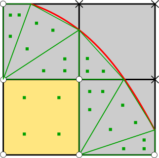
Figure 2. Illustration of the DOFs of the ${\mathcal{V}}_{h}^{\mathrm{ag}}$ space in the patch of cells highlighted in blue in Fig. 1b (which contains cut cells). Circles represent well-posed DOFs and crosses represent ill-posed ones. Ill-posed DOFs do not take arbitrary values, their values are actually defined via a suitable discrete extension operator defined in terms of linear constraints on the interior DOFs of the root cell of the aggregate. Cells $T\in\mathcal{T}_{h}$ are shown in black and sub-meshes for integration are shown in green. Small green squares represent numerical integration quadrature points. The DOFs and quadrature points shown are selected to illustrate the construction. They might not reflect their actual number (and spatial position) in the numerical experiments.

3.3. History variables discretization (via discontinuous Lagrangian FE spaces)

In the context of robust, $h$-adaptive, embedded FE solvers, the representation of constitutive model history variables as fields becomes essential (for reasons made clear along the rest of the section). With a representation as a field of the history variable, we can evaluate these quantities in whatever point of the domain, rather than a mere data array with values on quadrature points for numerical integration (as it is commonly implemented in nonlinear solid mechanics codes). For such representation, we choose a cell-wise polynomial, discontinuous FE space. In particular, the approximation of history variables is made by functions of a standard discontinuous Lagrangian FE space on the background mesh, defined as

$${\mathcal{V}}_{h}^{-,{\mathrm{std}}}(\mathcal{T}_{h}^{{\mathrm{act}}})\doteq\{v\in{{L}^{2}}({\Omega})\,:\,v|_{T}\in{\mathcal{V}}_{k}(T)\text{ for any }T\in\mathcal{T}_{h}^{{\mathrm{act}}}\}.$$ (7)

This space is also implemented using the nodal Lagrangian basis for ${\mathcal{Q}}_{k}(T)$ and a local-to-global DOF map. However, as there is no required inter-cell continuity in ${\mathcal{V}}_{h}^{-,{\mathrm{std}}}(\mathcal{T}_{h}^{{\mathrm{act}}})$, there is no need to glue DOFs belonging to the interface of neighbouring cells. As a result, nodes can be placed anywhere within the cell (any $\boldsymbol{x}^{i}_{T}\in T$ is valid). In the case of non-conforming meshes, linear constraints on hanging VEFs are not required either. Given this flexibility, we choose $\boldsymbol{x}^{i}_{T}$, for all active cells (i.e. both interior and cut cells), to be the location of the quadrature points used for the numerical integration in the interior cells, i.e. the tensor product of 1D Gauss quadratures; see, e.g. Fig. 3a. Since this is the quadrature rule used for the numerical integration of the discrete operator in interior cells, in such kind of cells, the history variables are already available for numerical integration once they are computed (no extra interpolation is required).

In cut cells it is also possible to choose a discontinuous space defined on the sub-mesh to represent history variables, that is, to consider ${\mathcal{V}}_{h}^{-,{\mathrm{std}}}(\mathcal{T}_{h}^{{\mathrm{int}}})$ as the approximating space. With this choice, the degrees of freedom in all cells (not only interior but also in cut ones) are the nodal values on the quadrature points.

However, there are a number of advantages of the representation that relies on the background mesh over this latter approach:

1. First, we avoid the permanent storage of history variables in all integration points of cut cells (which become a very high number of points, specially in 3D). Instead, the value of history variables in all integration points of cut cells is interpolated locally at each cell.

2. Second, when the background mesh is adapted (either refined and/or coarsened), a new integration mesh, and thus a new set of integration points, results from the intersection of the boundary of the domain and the adapted mesh. Thus, one needs the value of the history variables on this new set of points, while transferring functions from the original mesh to the adapted one. While this transfer operator can easily be computed in tree-based mesh refinement, it is much more involved between general unstructured meshes (as the ones in the sub-triangulation).

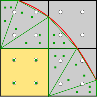
a Discontinuous standard FE space.

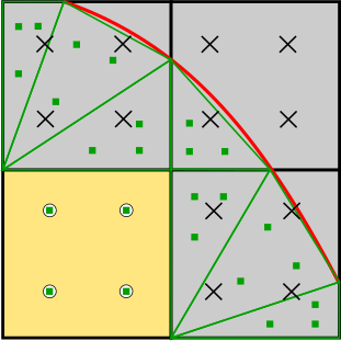
b Discontinuous agFE space.

Figure 3. Two possible choices for the DOFs of the FE space used to approximate the history variables. Circles represent DOFs which may take arbitrary values, while crosses, DOFs whose values actually depend on the interior DOFs of the root cell of the aggregate via suitably-defined linear constraints.

Another option available to deal with cut cells is to also use agFE spaces with discrete extension operators for history variables. This is not required to have a well-posed problem. Because history variables are updated from the displacements (and eventually pressures), their DOF values are not computed solving a linear system and thus there is no actual need to classify them as well-posed or ill-posed for better conditioning. However, using an agFE field representation we can leverage the same abstract software workflow both for the primal and internal variables, with a further reduction of computational cost in mind. Rather than computing history variables in cut cells, as it is done when ${\mathcal{V}}_{h}^{-,{\mathrm{std}}}(\mathcal{T}_{h}^{{\mathrm{act}}})$ is considered (values at circles in Fig. 3a), they are defined by the constraints (6) (which give values at crosses in Fig. 3b). We have actually observed that there is a slight reduction in total computing time, as the application of the constraints in (6) to obtain history values in cut cells is faster than computing history variables from displacements, but the gain is a minor fraction of the total computation. We have performed a test, reported in Sect. 6.2, to verify that both options result in similar accuracy for the representation of stresses. In this case the approximating space can simply be defined as:

$${\mathcal{V}}_{h}^{{\mathrm{-,ag}}}(\mathcal{T}_{h}^{{\mathrm{ag}}})\doteq\{v\in{{L}^{2}}({\Omega})\,:\,v|_{T}\in{\mathcal{V}}_{k}(T)\text{ for any }T\in\mathcal{T}_{h}^{{\mathrm{ag}}}\}.$$ (8)

3.4. Transfer operators among meshes

During the adaptive refinement loop, the spaces described above keep changing and therefore state and constitutive variables must be properly transferred among meshes. To this end, we use the standard nodal interpolation and $L^{2}$-projection operators for refinement and coarsening, resp., see e.g. [31].

However, in an embedded setting, under the presence of cut cells and aggregates, a somewhat specialized treatment is required. Since the refinement of a cut cell can lead to interior cells, the nodal interpolation must also be computed for refined cut cells. However, when refining a cut cell, only the interpolated DOFs of the refined interior cells are used, since the (ill-posed) ones of the refined cut cells are defined using the constraints in (the adapted) ${\mathcal{V}}_{h}^{\mathrm{ag}}$. This applies both for FE functions in ${\mathcal{V}}_{h}^{{\mathrm{ag}}}(\mathcal{T}_{h}^{{\mathrm{ag}}})$ and ${\mathcal{V}}_{h}^{{\mathrm{-,ag}}}(\mathcal{T}_{h}^{{\mathrm{ag}}}$). For FE functions in ${\mathcal{V}}_{h}^{-,{\mathrm{std}}}$, we use nodal interpolation to compute the values of the DOFs of all active children cells of a refined cut cell.

4. The nonlinear problem and its solution

In this section we describe the final discrete problem to be solved and the strategy we developed to perform this task. As usual, the nonlinear problem is solved by gradually increasing the external loads instead of directly looking for the final equilibrium. The load increment discretization is described in Sect. 4.1 and the solution of the nonlinear problem at each step is discussed in Sect. 4.2.

4.1. Pseudo-time discretization

The final nonlinear discrete problem defined below is obtained introducing a pseudo-time discretization, which describes the sequential increment of external loads or correction of boundary conditions to reach the final desired ones. Each component of the displacement field is approximated by a function $\boldsymbol{u}_{h}\in\mathbf{V}_{h}\doteq\left({\mathcal{V}}_{h}^{\mathrm{ag}}\right)^{d}$ (the Lagrangian agFE space of order $k$) and the internal variable is approximated by $\alpha_{h}\in{\mathcal{V}}_{h}^{\mathrm{-,ag}}$ (the discontinuous Lagrangian agFE).

Given the history variable $\alpha_{h}^{n}$ at step $n$, the discretization of the irreducible formulation (1) at load increment $n+1$ reads as follows: find $\boldsymbol{u}_{h}^{n+1}\in\mathbf{V}_{h}$ and $\alpha^{n+1}_{h}\in{\mathcal{V}}_{h}^{\mathrm{-,ag}}$ such that

$$\langle\boldsymbol{\mathcal{R}}(\alpha^{n}_{h};\boldsymbol{u}_{h}^{n+1}),\boldsymbol{v}_{h}\rangle=0,$$ (9)

for any $\boldsymbol{v}_{h}\in\mathbf{V}_{h}$, where

$$\langle\boldsymbol{\mathcal{R}}(\alpha_{h};\boldsymbol{u}_{h}),\boldsymbol{v}_{h}\rangle={\mathcal{A}}(\alpha_{h};\boldsymbol{u}_{h},\boldsymbol{v}_{h})+{\mathcal{B}}(\alpha_{h};\boldsymbol{u}_{h},\boldsymbol{v}_{h})-\mathcal{F}(\alpha_{h};\boldsymbol{v}_{h}),$$ (10)

and

$${\mathcal{A}}(\alpha_{h};\boldsymbol{u}_{h},\boldsymbol{v}_{h}) =\int_{{\Omega}}{\boldsymbol{\nabla}\,\boldsymbol{v}_{h}:\boldsymbol{\sigma}(\boldsymbol{u}_{h},\alpha_{h})}\,d{\Omega},$$ (11)

$${\mathcal{B}}(\alpha_{h};\boldsymbol{u}_{h},\boldsymbol{v}_{h}) =\int_{\Gamma_{\rm D}}{{\boldsymbol{n}}\cdot\boldsymbol{\sigma}(\boldsymbol{v}_{h},\alpha_{h})\cdot\boldsymbol{u}_{h}}\,d\Gamma_{\rm D}-\int_{\Gamma_{\rm D}}{{\boldsymbol{n}}\cdot\boldsymbol{\sigma}(\boldsymbol{u}_{h},\alpha_{h})\cdot\boldsymbol{v}_{h}}\,d\Gamma_{\rm D}-\int_{\Gamma_{\rm D}}{\beta\boldsymbol{v}_{h}\cdot\boldsymbol{u}_{h}}\,d\Gamma_{\rm D},$$ (12)

$$\mathcal{F}(\alpha_{h};\boldsymbol{v}_{h}) =\int_{{\Omega}}{\boldsymbol{v}_{h}\cdot\boldsymbol{f}^{n+1}}\,d{\Omega}+\int_{\Gamma_{\rm N}}{\boldsymbol{t}^{n+1}\cdot\boldsymbol{v}_{h}}\,d\Gamma_{\rm N}$$ (13)

$$-\int_{\Gamma_{\rm D}}{{\boldsymbol{n}}\cdot\boldsymbol{\sigma}(\boldsymbol{v}_{h},\alpha_{h})\cdot\overline{\boldsymbol{u}}^{n+1}}\,d\Gamma_{\rm D}-\int_{\Gamma_{\rm D}}{\beta\boldsymbol{v}_{h}\cdot\overline{\boldsymbol{u}}^{n+1}}\,d\Gamma_{\rm D}.$$ (14)

When the mixed formulation is considered, we use the Taylor-Hood mixed FE, but other stable pairs can be considered; we refer to [9] for the analysis of some aggregated inf-sup stable pairs. In this case, the displacement components space $\mathbf{V}_{h}$ and the pressure space $\mathbf{Q}_{h}$ are a second order and first order aggregated Lagrangian FE space, resp. Then, the final discrete problem to be solved at each step is to find $\boldsymbol{u}_{h}^{n+1}\in\mathbf{V}_{h}$, $p_{h}^{n+1}\in\mathbf{Q}_{h}$ and $\alpha^{n+1}_{h}\in{\mathcal{V}}_{h}^{\mathrm{-,ag}}$ such that

$$\langle\boldsymbol{\mathcal{R}}(\alpha^{n}_{h};\boldsymbol{u}_{h}^{n+1},p^{n+1}_{h}),(\boldsymbol{v}_{h},q_{h})\rangle=0,$$ (15)

for any $\boldsymbol{v}_{h}\in\mathbf{V}_{h}$ and $q_{h}\in\mathbf{Q}_{h}$ where

$$\langle\boldsymbol{\mathcal{R}}(\alpha_{h};\boldsymbol{u}_{h},p_{h}),(\boldsymbol{v}_{h},q_{h})\rangle={\mathcal{A}}(\alpha_{h};\boldsymbol{u}_{h},p_{h},\boldsymbol{v}_{h},q_{h})+{\mathcal{B}}(\alpha_{h};\boldsymbol{u}_{h},p_{h},\boldsymbol{v}_{h},q_{h})-\mathcal{F}(\alpha_{h};\boldsymbol{v}_{h},q_{h})),$$ (16)

the forms ${\mathcal{B}}$ and $\mathcal{F}$ are defined as in (12) and (14) but with $\boldsymbol{\sigma}(\boldsymbol{u}_{h},p_{h},\alpha_{h})$ and ${\mathcal{A}}$ is (11) plus the terms

$$\int_{{\Omega}}{\kappa^{-1}q_{h}p_{h}}\,d{\Omega}-\int_{{\Omega}}{q_{h}\nabla\cdot\boldsymbol{u}_{h}}\,d{\Omega}.$$ (17)

Note that (12) includes Nitsche’s method [7, 6, 8] terms to impose Dirichlet boundary conditions. $\beta>0$ is a mesh-dependent parameter that needs to be large enough to ensure the positivity of the final discrete problem (after linearization). For linear elliptic problems, one takes $\beta=\beta_{0}h_{T}^{-1}$ with a constant $\beta_{0}$ large enough. When the Dirichlet boundary is conforming to the mesh, as in the numerical experiments in Sect. 6, we use a strong imposition of boundary conditions, and the Nitsche terms are switched off. The history variable $\alpha^{n+1}_{h}$ is a by-product of the evaluation of the stresses with $\boldsymbol{u}_{h}^{n+1}$ and $p_{h}^{n+1}$ (see below).

4.2. Linearization and solution

The Newton-Raphson algorithm is used to solve (9) and (15), due to its quadratic rate of asymptotic convergence. It consists of an iterative loop performed at each step in which the displacement is updated as

$$\boldsymbol{u}_{h}^{n+1,i+1}=\boldsymbol{u}_{h}^{n+1,i}+\omega^{i}\delta\boldsymbol{u}_{h}^{i},$$ (18)

where $i$ denotes the nonlinear solver iteration counter, $\boldsymbol{u}_{h}^{n+1,i+1}$ and $\boldsymbol{u}_{h}^{n+1,i}$ denote the value of the displacement field obtained for the $(i+1)-th$ and $(i)-th$ nonlinear iterations, resp., and $0<\omega^{i}\leq 1$ is a relaxation parameter determined by a standard line search with cubic backtracking [32]. The increment $\delta\boldsymbol{u}_{h}^{i}$ is obtained solving the tangent problem

$$D\boldsymbol{\mathcal{R}}(\alpha^{n}_{h};\boldsymbol{u}_{h}^{n+1,i})[\delta\boldsymbol{u}_{h}^{i}]=-\boldsymbol{\mathcal{R}}(\alpha^{n}_{h};\boldsymbol{u}_{h}^{n+1,i})\ ,$$ (19)

where the Jacobian, $D\boldsymbol{\mathcal{R}}$, is computed from (10) or (16), and requires differentiating $\boldsymbol{\sigma}$, which is implemented using the constitutive tangent tensor $\mathbb{C}^{\rm ep}$ see, e.g. [24, Section 7].

The combination of these techniques (Newton-Raphson with line-search) is a well-known and powerful technique for the solution of strongly nonlinear problems. Therefore, the only point that deserves attention here is how the use of embedded methods with the choice of approximating spaces discussed in Sect. 3 affects the evaluation of the Jacobian and the residual. Both are required to determine the increment from (19) and the residual is also required at each line search iteration. In general, the required number of line-search iterations is difficult to determine a priori, as it depends on several factors, such as the complexity of the geometry, the loading process, and the material properties, among others.

The system (19) is assembled for the well-posed DOFs. Once solved, constrained DOFs in $\delta\boldsymbol{u}_{h}^{i}$ are computed using (6), that is, values at crosses are updated from values at circles in Fig. 2. The update in (18) is a functional one, that is, performed for all DOFs defining functions $\boldsymbol{u}_{h}\in\mathbf{V}_{h}$ (whose components are in ${\mathcal{V}}_{h}^{\mathrm{ag}}$).

In order to evaluate the Jacobian and/or the residual, we need to compute the stresses (see (11) to (14)) evaluating the function $\boldsymbol{\sigma}$ in (2), which includes the projection onto the space of admissible stresses (executing the radial return algorithm). This procedure is executed at the integration points (green points in Fig. 2 and Fig. 3). In interior cells, the input required for this computation is $\boldsymbol{u}_{h}^{n+1,i}$ and $\alpha^{n}_{h}$ at integration points. Displacements are interpolated at the integration points while history variable values at the integration points are already stored; DOFs and quadrature points coincide. As a by-product of the stress projection, updated values of the internal variable $\alpha^{n+1}_{h}$ DOFs are obtained.

In cut cells, the situation is different, since history variable DOFs (circles in Fig. 3a) are not quadrature point values (green points in Fig. 2 and Fig. 3). Thus, $\alpha^{n}_{h}$ are obtained by interpolation (from circles and crosses to green points in Fig. 2 and Fig. 3, resp.). At these integration points, stresses are computed with the interpolated values, i.e. $\boldsymbol{\sigma}(\boldsymbol{u}_{h}^{n+1,i},\alpha^{n})$. After convergence of the nonlinear solver, the values of the history variables at the integration points (green points in Fig. 3) are discarded and computed at the DOFs locations (circles in Fig. 3a) to obtain $\alpha^{n+1}$.

5. Building hierarchically adapted meshes during incremental load-stepping

Alg. 1 sketches our strategy to bridge load-stepping and dynamic AMR in an embedded setting. The algorithm is designed to accurately capture the inelastic behavior of the embedded solid in the course of a load-increment simulation, while keeping the computational demands within acceptable margins. To this end, the algorithm exposes a set of user-defined parameters that play a role in striking a balance among controlling that the global error does not blow up during the simulation and keeping computational requirements within acceptable margins. Up to the authors’ knowledge, the approaches proposed in the literature to bridge load-stepping and AMR (see, e.g. [15, 16]), do not seem to pay a careful attention to this ingredient, advocating instead for simple strategies in which the mesh is adapted either once or at most once at each step (regardless of the global error). Our experience reveals that a proper tuning of the parameters of Alg. 1 for each problem at hand can have a significant impact on the balance struck in practice among accuracy and computational cost.

1 Generate initial background mesh (uniformly refined octree + multiple sweeps of coarsening of exterior cells)

2

3current_load_step$\leftarrow$ 1

4 while current_load_step $<$ num_load_steps do

5      Update current load/displacement

6      Solve nonlinear problem [see (10) or (16)]

7      if  current_load_step modulo amr_step_freq $\equiv 0$  then

8           Compute $\eta_{T}$, $T\in\mathcal{T}_{h}^{{\mathrm{act}}}$ and $\eta_{G}$ [see (20)]

9           current_amr_step $\leftarrow$ 1

10           while ($\eta_{G}$ $>$ $\eta_{G}^{\text{max}}$) and (current_amr_step < num_amr_steps) do

11                Retrieve state and constitutive model variables of current load step

12               

13               Refine/coarsen fraction $\theta_{r}$/$\theta_{c}$ of $|\mathcal{T}_{h}^{{\mathrm{act}}}|$ with the largest/smallest $\eta_{T}$

14               Intersect domain with adapted background mesh and generate aggregates

15               Transfer variables to the new mesh [see Sect. 3.4]

16               

17               Redistribute mesh and migrate variables among tasks

18               

19               Intersect domain with adapted background mesh and generate aggregates

20               Solve nonlinear problem [see (10) or (16)]

21                Compute $\eta_{T}$, $T\in\mathcal{T}_{h}^{{\mathrm{act}}}$ and $\eta_{G}$ [see (20)]

22                current_amr_step $\leftarrow$ current_amr_step + 1

23               

24          

25      current_load_step $\leftarrow$ current_load_step + 1

26     

Algorithm 1 Load-stepping and parallel AMR in an embedded setting.

The inner AMR loop in Alg. 1 combines (a-posteriori) local and global error estimators. These are denoted as $\eta_{T}$, for $T\in\mathcal{T}_{h}^{{\mathrm{act}}}$, and $\eta_{G}$, resp., in Alg. 1. Local error estimators are used in order to decide which cells are marked for refinement and coarsening among two consecutive meshes in the hierarchy; see line 1. In particular, for that purpose, given user-defined refinement and coarsening fractions, denoted by $\theta_{r}$ and $\theta_{c}$, resp., we refine the fraction $\theta_{r}$ of the total number of active cells with the largest local error estimator, and coarsen the fraction $\theta_{c}$ with the smallest local error estimators. We note that the generation of the initial background mesh in line 1 applies, to a uniformly refined octree, multiple sweeps of coarsening of exterior cells till two consecutive meshes are equivalent. This pursues to minimize the number of exterior cells of the background mesh . The experiments in Sect. 6 reveal that this strategy is effective in achieving large percentages of active cells versus total number of cells along the whole simulation.

In Sect. 6, for simplicity, we consider a residual-based a-posteriori error estimator grounded on the seminal works [33, 34, 35] (although more complex local error estimators can readily be used in our framework). This kind of error estimators are well-known, so that we refer the reader to these references for a detailed definition. It is worth mentioning, however, that in an embedded setting, the implementation of this algorithm requires integration on “cut faces” (i.e. faces of the cut cell sub-mesh of simplices that enclose $T\cap\Omega$; see Fig. 2), as these error estimators involve the evaluation of integrals (of the jump of the normal stresses) on the boundary of the cells. On the other hand, in Sect. 6, we consider the following estimation of the relative global error

$$\eta_{G}=\sqrt{\frac{\sum_{T}\eta_{T}^{2}}{{\mathcal{A}}(\boldsymbol{u}_{h},\boldsymbol{u}_{h})}},$$ (20)

where ${\mathcal{A}}(\boldsymbol{u}_{h},\boldsymbol{u}_{h})$ (i.e. $||\boldsymbol{u}_{h}||_{\mathcal{A}}^{2}$) denotes the (squared) discrete energy norm defined in (11). This definition of the estimated global error was proposed to drive mesh adaptivity for linear elliptic problems in [36]. This definition has the benefit of being dimensionless, in contrast to, e.g. using the Euclidean norm of the vector of nodal values of $\boldsymbol{u}_{h}$ in the denominator [16].

The estimated global error $\eta_{G}$, combined with a user-defined upper threshold, denoted as $\eta_{G}^{\text{max}}$ in Alg. 1, defines a mesh acceptability criterion that we are willing to fulfill at the final load, but also plays a role along the simulation by controlling how many adaptation steps we perform within each load step. The requirement on $\eta_{G}$ strictly below $\eta_{G}^{\text{max}}$ is relaxed with the so-called num_amr_steps parameter; see line 1. Essentially, in each load step, a maximum of num_amr_steps mesh adaptation steps are allowed. We note that the execution of the inner loop in Alg. 1 depends on the user-configurable amr_step_freq parameter, the frequency that controls how many load steps the user allows the simulation to run without adapting the mesh.

6. Numerical experiments

The main purpose of this section is to showcase the high suitability of the algorithmic framework proposed in order to efficiently deal, both in terms of numerical accuracy and computational performance, with large-scale elasto-plasticity problems with localized effects posed over complex geometries. First, we have conducted a set of validation tests of the framework against experimental benchmarks with results available in the literature and problems with known analytical solution. In particular, we considered the 2D nearly-incompressible plane strain Cook’s Membrane (see, e.g. [37]), an internally pressurized thick cylinder (see, e.g. [16] and [24, Section 7.5.1]) and the stretching of a 3D perforated rectangular plate (see [38, 24]). We have been able to confirm the correctness of the algorithms at hand when applied to these benchmarks, for which our results match the ones in the literature accurately. Among these examples, for conciseness, we only present here the results of the internally pressurized thick cylinder in Sect. 6.2. In particular, this section compares the accuracy of both possibilities for the approximation of the history variables discussed in Sect. 3.3. Before that, we describe the experimental environment (hardware and software) and the setup common to all experiments in Sect. 6.1.

Moving to complex geometries, we consider in Sect. 6.3 the traction of two 3D periodic lattice-type geometries representative of the ones which are enabled by AM technology; see, e.g., [39]. Although there is no analytical solution at our disposal for such complex elasto-plasticity problems, the focus here is to evaluate the ability of the building blocks of Alg. 1 to resolve the underlying physics while keeping the size of the discrete problem within acceptable margins. Later on, in Sect. 6.4, we consider the deformation of a cantilever beam with spherical hollows subject to a vertical uniformly distributed load applied in the upper face. This section also reports the results of a strong scalability study. The goal is to evaluate the ability of the framework to efficiently reduce computational times with increasing computational resources (cores and memory) when deployed on a parallel supercomputer.

We stress that the problems in this section have been judiciously selected so that they have features that potentially pose significant challenges to CAD/CAE frameworks: intricate geometries, high nonlinearity, long and thin regions with strong localization (weak links), and varying amount of material per unit of volume. These features cause non-symmetric refinement patterns, potential load unbalance to be addressed dynamically in a parallel setting, and nonlinearity onset on the unfitted boundary, among others. The main goal of the section is to reassure that the algorithmic framework proposed is able to promisingly deal with all this complexity.

6.1. Experimental environment and setup common to all experiments

All numerical experiments are carried out on a parallel, distributed-memory environment. In particular, we used two different supercomputers:

• Marenostrum-IV (MN-IV) [40], hosted by the Barcelona Supercomputing Centre. MN-IV is a petascale machine with 3456 nodes distributed in 45 racks, interconnected with the Intel OPA HPC network. Each node has 2x Intel Xeon Platinum 8160 multi-core cores, with 24 cores each (i.e. 48 cores per node), and 96 GB of RAM.

• NCI-Gadi [41], hosted by the Australian National Computational Infrastructure Agency (NCI), is a petascale machine with 3024 nodes, each containing 2x 24-core Intel Xeon Scalable Cascade Lake cores and 192 GB of RAM. All nodes are interconnected via Mellanox Technologies’ latest generation HDR InfiniBand technology.

The algorithms at hand have been implemented using the tools provided by FEMPAR [42], an open source Object-Oriented (OO) Fortran200X scientific software package for the High Performance Computing (HPC) simulation of complex multiphysics problems governed by Partial Differential Equations at large scales. Among others, FEMPAR provides scalable implementations of the algorithms in charge of generating the AgFEM aggregates, and handling the linear constraints required in order to preserve conformity on non-conforming octrees and make the problem better conditioned, all in a parallel distributed framework; see  [10] for a detailed presentation of these algorithms. We configure FEMPAR so that it uses p4est as its specialized forest-of-octrees meshing engine [5]. In order to solve the nonlinear problem (see Sect. 4) we exploit the algorithms available in the Scalable Nonlinear Equations Solver SNES, a module available in PETSc [22]. FEMPAR provides to PETSc all data structures required to properly handle the life cycle of the nonlinear solver. FEMPAR [43] was linked against p4est v2.2 [28], PETSc v3.12.4 [22] and Qhull v2015.2 [44], a library to compute convex hulls and Delaunay triangulations. All software is compiled with Intel v.18.0.5 in MN-IV, Intel v.19.1.0.166 in NCI-Gadi. All floating-point operations are performed in IEEE double precision.

In all experiments of the section the geometry is built using a cuboid $[0,L]^{d}$ as artificial domain, discretized with a background octree mesh of this domain. This mesh is then intersected with level-set functions, which are used to describe the boundary of the embedded domain. To keep the presentation concise, we do not include the mathematical definition of these functions. We refer the reader to, e.g. [6, 11], and references therein for a detailed definition. Table 1 summarizes the main parameters and computational strategies used in the experiments. The parameters of Alg. 1 are particularized for every test, and thus are presented in the section corresponding to each test.

Description	Considered methods/values
Model formulation	Irreducible formulation
Background mesh	Single quadtree (2D) or octree (3D)
FE space state vars	First order agFE space
FE space history vars	First order discontinuous agFE space
SNES - nonlinear solver	Newton + cubic backtracking line search
SNES stopping criterion	$\|\mathbf{r}\|_{2}<10^{-12}$
	$\|\mathbf{r}\|_{2}/\|\mathbf{r_{0}}\|_{2}<10^{-12}$
KSP - linear solver	Preconditioned conjugate gradient
Parallel preconditioner	Smoothed-aggregation GAMG (PETSc)
KSP stopping criterion	$\|\mathbf{r}\|_{2}/\|\mathbf{b}\|_{2}<10^{-12}$

Table 1. Summary of main parameters and computational strategies.

6.2. Internally pressurized thick cylinder

In this section we present selected results when applying the framework to an elasto-plastic problem with known analytical solution, namely a long metallic thick-walled cylinder subjected to internal pressure. The main goal is to evaluate the impact of the FE space used for representing the internal variables of the constitutive model, i.e. ${\mathcal{V}}_{h}^{-,{\mathrm{std}}}$ versus ${\mathcal{V}}_{h}^{{\mathrm{-,ag}}}$, on the accuracy of the computed stresses. The main feature of this test is that, once the internal pressure reaches its maximum value, the whole domain is in the plastic regime.

The analysis of the internally pressurized thick cylinder is carried out assuming plane strain conditions. As a consequence, only one quarter of the cylinder, with the appropriate boundary conditions, is required to represent the full test (see [16] and [24, Section 7.5.1]); see Fig. 4a for the description of the geometry and boundary conditions. The pressure $P$, prescribed in the inner surface, is incremented gradually until the limit load is reached. While the internal pressure is small, the entire cylinder will remain elastic. However, as $P$ increases, the cylinder begins to yield from the inner surface $r=a$. Then, the yielded region expands outwards forming a cylindrical plastic front. The analytical displacement solution in polar coordinates for both, elastic and plastic regions, as a function of $r$, can be found in [45] and [46].

We set the inner radius $a=100\,\text{mm}$, and outer radius $b=200\,\text{mm}$ and the side of the artificial domain has a length $L=b$. In order to capture the behavior of the material, we considered a compressible perfect plastic material with Young’s modulus $E=210\,\text{GPa}$, Poisson’s ratio $\nu=0.30$, and yield stress $\sigma_{y}=240\,\text{MPa}$. We considered as total internal pressure $P=0.19\,\text{GPa}$, discretized into 11 load steps.

In Fig. 4b we report the $L^{2}$-norm relative error in the radial ($\sigma_{{r}{r}}$) and hoop stress ($\sigma_{{\theta}{\theta}}$) components as a function of the number of DOFs in the final state of the mesh. The different points in the figure were generated using a sequence of uniformly refined meshes, starting from a $4\times 4$ uniform mesh at the left-most point refined six times to reach the right-most one. The error of the radial stress decays as $\mathcal{O}(h^{-1})$, i.e. as $\mathcal{O}(n^{-1/2})$, with $n$ the number of DOFs, as it can be expected for an elliptic problem with a smooth solution approximated by linear functions. The error of the hoop stress also decays as $\mathcal{O}(n^{-1/2})$ for coarse meshes but the rate decreases for finer ones. Because the exact hoop stress is not regular [46], convergence can be expected but its rate cannot be predicted. In any case, the main conclusion that can be extracted from the experiment is that both options for the FE space representing the history variables result in similar accuracy for the representation of stresses. As a slight reduction of computational times was observed for ${\mathcal{V}}_{h}^{{\mathrm{-,ag}}}$, we stick into this FE space for the rest of the experiments in the section.

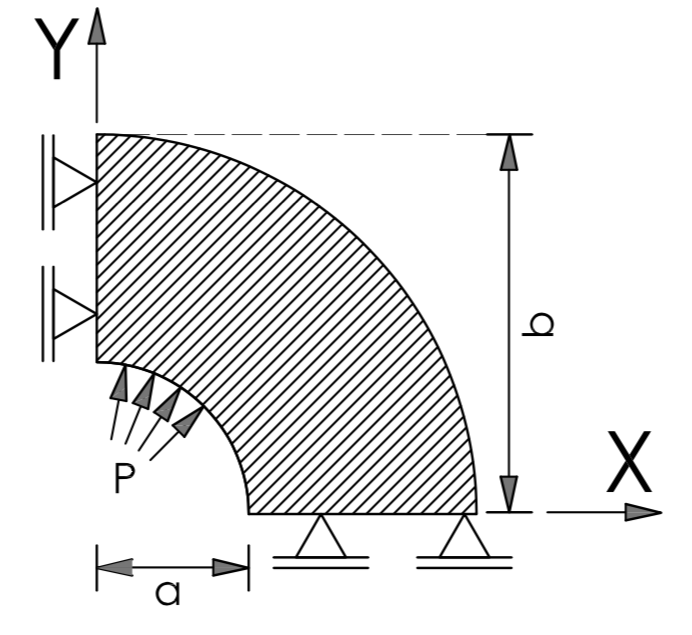
a

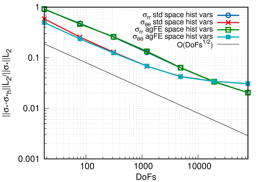
b

Figure 4. Internally pressurized thick cylinder: (A) Geometry description and boundary conditions. (B) Convergence of radial ($\sigma_{{r}{r}}$) and hoop ($\sigma_{{\theta}{\theta}}$) stresses. ${\mathcal{V}}_{h}^{-,{\mathrm{std}}}$ (standard space for history variables) versus ${\mathcal{V}}_{h}^{{\mathrm{-,ag}}}$ (agFE space for history variables).

6.3. Traction of complex 3D lattice-type structures

After validating the framework against standard benchmarks, we move to more intricate geometries with the aim of verifying the ability of the building blocks of Alg. 1 to accurately resolve the underlying physics while keeping computational resources (e.g. number of cells/DOFs) within acceptable margins. To this end, we consider traction tests performed on two different 3D periodic structures representative of the ones that are enabled by AM technology [39]; see Fig. 5. This kind of structures are geometrically intricate, difficult to discretize with body-fitted mesh generators. This complexity triggers also a nontrivial physical behavior with long and thin regions (weak links) where localization may occur. Besides, the onset of nonlinearity is located on the unfitted boundary, putting further stress on the adaptive cut cell FE formulation. The two geometries considered herein differ in the amount of material per unit of volume (the ratio between material and empty space), resulting in different refinement patterns and geometric distribution of plastic regions.

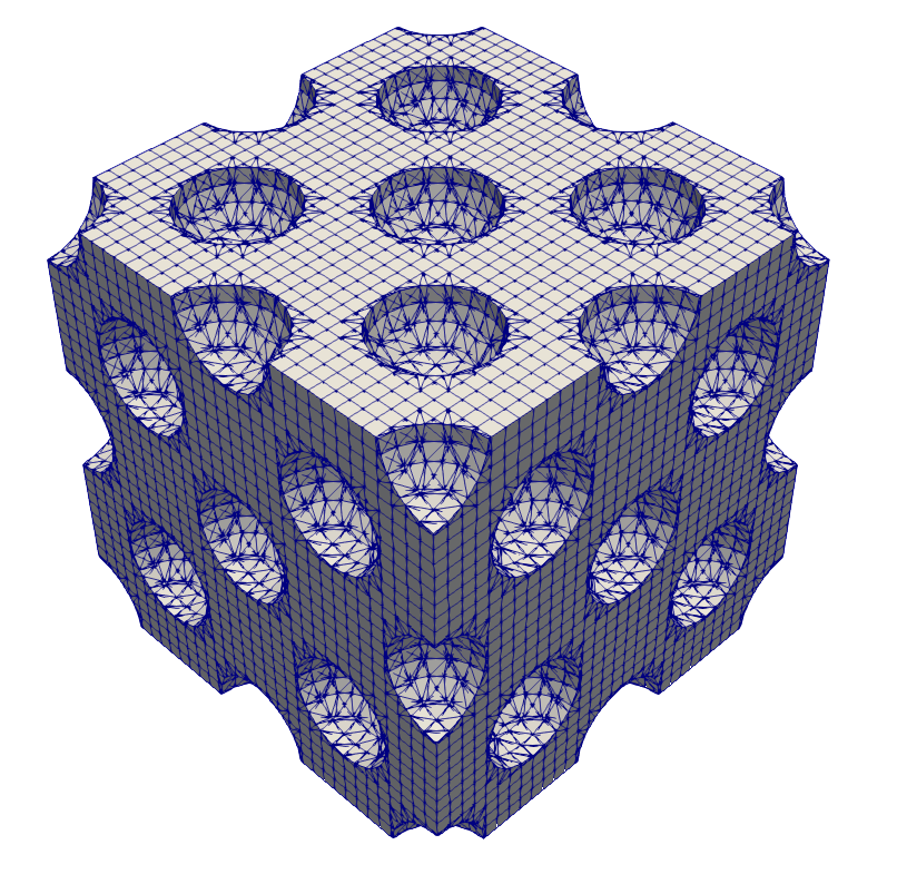
a

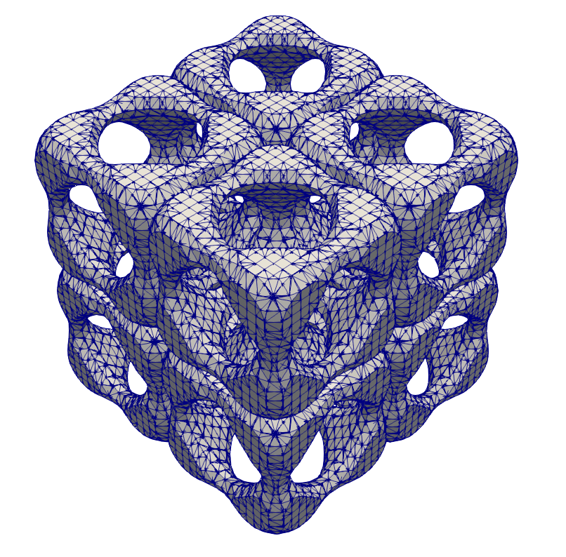
b

Figure 5. 3D geometry and initial FE mesh ($\mathcal{T}_{h}^{{\mathrm{int}}}$) of (A) hollow and (B) lattice structures.

The first geometry is a sample of material that consists of homogeneous medium with spherical hollows of radius $0.12\,\text{m}$, organized in a periodic face-centered cubic (FCC) lattice structure of side $L/2$. [47]; see Fig. 5a. The second geometry is a lattice structure obtained by repetitive Boolean operations (copy, translate and union) of a single structural block described by level-set functions given in [6]; see Fig. 5b. The artificial domain is the unitary cuboid with side length $L=1\,\text{m}$ in both cases. This domain can be simply discretized by a single octree. Fig. 5 also shows the initial $\mathcal{T}_{h}^{{\mathrm{int}}}$ meshes, i.e. the ones which result from the intersection of the domain and the initial background meshes. The latter were in turn generated by uniform refinement of the root cell of the octree plus multiple sweeps of coarsening of exterior cells (see line 1 of Alg. 1). We note that the meshes shown include the tetrahedral subcells generated for integration purposes (excluding exterior cells), so that we can clearly see the shape of the boundaries. A body-fitted discretization of these geometries is not easy to generate but automatic with the unfitted method.

In both tests we considered the following material properties: Young modulus $E=70\,\text{GPa}$ and Poisson’s ratio $\nu=0.2$. The inelastic material behavior will be captured by an isotropic J2 plasticity model based on the particularization of the functions presented in Sect. 2.2. For the hardening evolution law, we consider a linear hardening ($K_{inf}=K_{0}=0$ and $\delta=0$), the yield threshold and the isotropic hardening factors being $\sigma_{y}=0.243\,\text{GPa}$ and $H=0.2\,\text{GPa}$, resp. On the other hand, boundary conditions are also similar. The structure is clamped at $x=0$ and the rest of the faces of the structures are traction-free. An horizontal displacement $\boldsymbol{u}_{x}=0.01\,\text{m}$ is incrementally imposed in $60$ uniform load steps at $x=L$ in the case of the hollow structure, while $\boldsymbol{u}_{x}=0.005\,\text{m}$ is incrementally imposed in $51$ uniform load steps at the same face in the lattice structure. We used Alg. 1 taking $\theta_{r}=0.1$ and $\theta_{c}=0.05$, and a constant $\eta_{G}^{\text{max}}=0.1$ along the whole simulation. Besides, we set amr_step_freq=4, and num_amr_steps=4.

In Fig. 6 we show the value of the J2 plasticity internal variable $\alpha$ once the full load has been applied to the corresponding structures. This is accompanied, in Fig. 7, with the associated mesh refinement pattern. For a better illustration, Figs. 7a and 7b also include exterior cells. We stress, though, that these cells do not actually carry DOFs in the unfitted method.

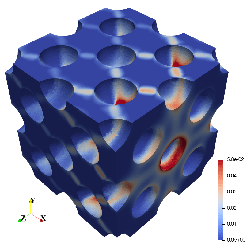
a

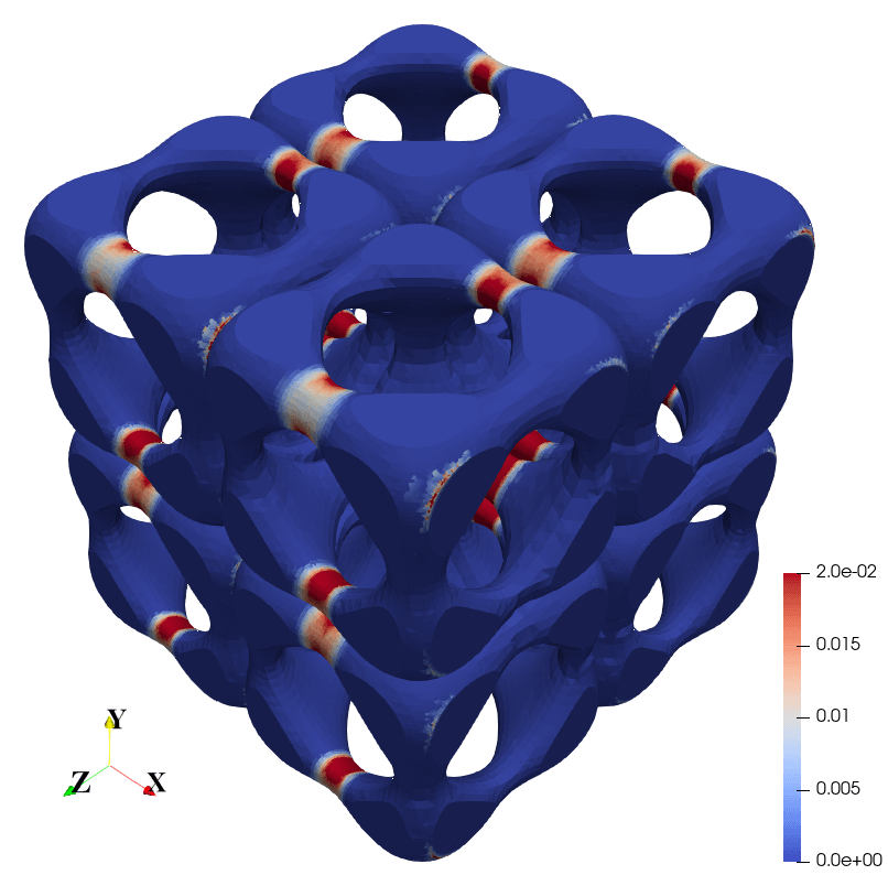
b

Figure 6. J2 Plasticity history variable $\alpha$ at the last load step in (A) hollow and (B) lattice structures.

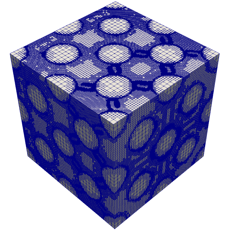
a

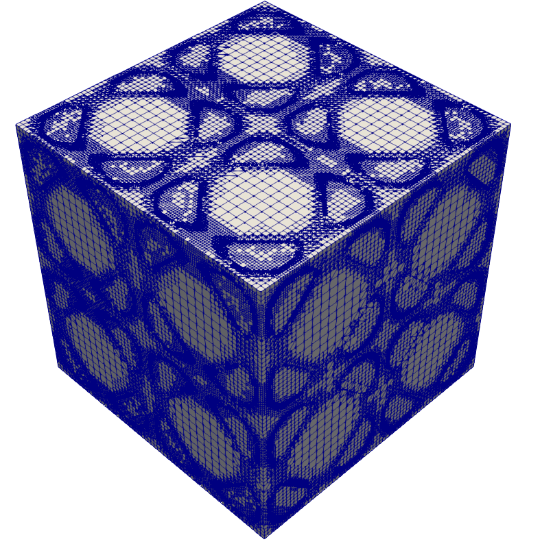
b

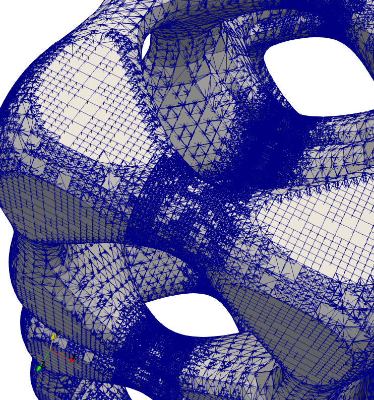
c

Figure 7. Mesh refinement pattern in (A) hollow and (B) lattice structures. (C) Close view of the mesh of the lattice structure.

Despite not having access to the exact solution, we can conclude that the results obtained are in a reasonable agreement with the physics underlying the problem at hand. The variable $\alpha$ can be interpreted as a measure of the evolution of the inelastic strains of the material. Regions where the stress states are mainly controlled by shear (i.e. involving a large deviatoric component) will yield large values of $\alpha$. Fig. 6 clearly reveals some localized regions with higher $\alpha$ values, with a particular spatial distribution which is consistent with the geometry of the structures and the applied loads. This effect is accompanied with a higher local mesh resolution in those areas, as can be observed in Fig. 7. In the hollow structure (Fig. 6a), some strain localization bands can be observed in regions between hollows. (Nevertheless the plastic regime has also spread through many other regions of the structure.) In contrast, in the lattice structure, shown in Fig. 6b, the plastic region is concentrated exclusively in the thin links of the structure.

In the sequel, for conciseness, we restrict the presentation of results to those of the hollow structure. The results obtained with the lattice structure are, in general qualitative terms, similar. In particular, in Fig. 8 we show the evolution of the error indicator $\eta_{G}$, while in Table 2, we report the number of DOFs and cells, and the fraction of active cells with respect to the total number of cells in the background mesh for each of the stages in-between mesh adaptations. The former quantity as reported in Table 2 (and in any of the tables herein) does not include those DOFs which are subject to multipoint linear constraints (i.e. hanging and ill-posed DOFs).

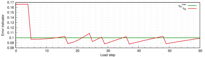
Figure 8. Evolution of the error indicator during loading (hollow structure).

Concept   \  load step	1-4	5-16	17-24	25-28	29-36	37-48	49-60
Free DOFs [M]	0.084	0.303	0.528	0.916	1.582	2.758	4.730
Total background mesh cells [M]	0.031	0.147	0.249	0.421	0.708	1.190	2.00
Active cells (% Total cells)	92.82	92.27	92.64	92.67	93.39	94.15	94.90
Accumulated AMR cycles	0	3	4	5	6	7	8
Average nonlinear iters. per load step	15	30	12	9	25	9	18

Table 2. Evolution of AMR cycles, size of the problem and (average) nonlinear iterations (hollow structure).

The number of cells and DOFs grow at a rate determined by the parameters of Alg. 1 and the growth of the error indicator; see Fig. 8 and Table 2. Mesh adaptations occur at steps 4, 16, 24, 28, 36 and 48. During the load steps in-between adaptations the mesh remains unchanged. Some relevant conclusions can be extracted out of these results. First, these results confirm that, as far as an error indicator-based mesh acceptability criterion is to be fulfilled, there is actually no need to adapt/redistribute the mesh at each load step, as, e.g., it is done in [15]. This in turn translates into significantly reduced computational times compared to other heuristic, non-error-driven strategies. This is indeed one of the main goals of Alg. 1. Second, as $\theta_{r}=0.1$, the ratio of active cells in the meshes corresponding to two consecutive adaptation cycles asymptotically converges to approximately 1.7, as only one mesh adaptation cycle is required to keep $\eta_{G}$ below $\eta_{G}^{\text{max}}$ when AMR is triggered. Third, during the whole simulation, the number of active cells is very close to the number of total cells. Some external cells are refined to satisfy the 2:1 balance constraint but their number is actually very small. Thus, these results confirm that, as far as one coarsens as much as possible exterior cells right at the beginning, they do not actually represent a source of overhead for the combined use of the unfitted method and AMR. Finally, in Table 2 we also report the average number of nonlinear Newton iterations required to solve the nonlinear problems at lines 1 and 1 in Alg. 1. This number is an indication of the difficulty of solving the nonlinear problem on a given mesh and, as it can be seen from Table 2, quite variable depending, among other factors, on the mesh adaptation patterns and the loading process.

6.4. 3D Cantilever Beam strong scalability test

In this section we present the results of a shear test of a geometrically complex 3D beam. The objective of this section is to evaluate the computational performance of Alg. 1 for problems with localized inelastic behavior. In particular, we are interested in evaluating and justifying the ability of Alg. 1 to efficiently exploit increasing computational resources (cores and memory) when deployed on a parallel supercomputer.

The problem consists of finding the displacement of a beam subject to a uniform load applied on the upper surface. The geometry is a homogeneous medium whose size is $L\times L/3\times L/3$ with spherical hollows of radius $0.116\,\text{m}$, arranged in a SC lattice of side $L/6$ [47], shown in Fig. 9, which also shows the initial mesh. The material properties correspond to a standard A-36 steel having $E=200\,\text{GPa}$ and $\nu=0.26$. The inelastic behavior is modeled with a linear isotropic J2 plasticity constitutive model, where $K_{inf}=K_{0}=0$ and $\delta=0$, and the yield threshold and the isotropic hardening factors being $\sigma_{y}=0.250\,\text{GPa}$ and $H=0.2\,\text{GPa}$, resp. Homogeneous Dirichlet boundary conditions are prescribed in $x=0$ and the rest of the faces are traction free, except the upper one (i.e. $y=L/3$) in which a linearly increasing traction from $0$ to $20\text{KN}/\text{m}^{2}$ is applied, discretized into $41$ load steps. We note that the imposition of this Neumann-type boundary condition requires the second integral in the right-hand side of (14) and thus involves the evaluation of integrals over cut faces. In Alg. 1, we set $\theta_{r}=0.07$, $\theta_{c}=0.03$, $\eta_{G}^{\text{max}}=0.06$, amr_step_freq=2, and num_amr_steps=4. Experimentation with this particular set of parameter values when applied to the same problem but coarser resolution meshes revealed that these were able to achieve a reasonable trade-off among all factors involved (compared to other possible a priori sensible choices). We show the localization at the maximum load step close to the clamped face in Fig. 10a (mesh refinement) and 10b (J2 isotropic plasticity history variable $\alpha$).

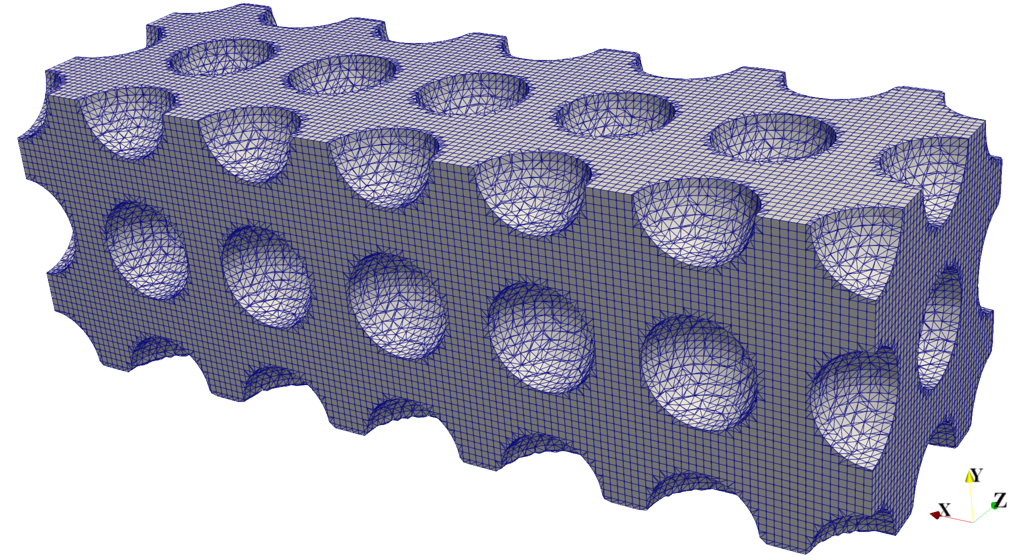
Figure 9. Geometry and initial mesh of the 3D Cantilever beam.

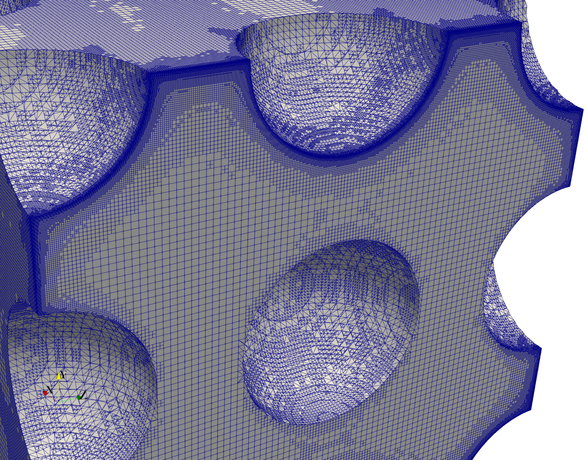
a

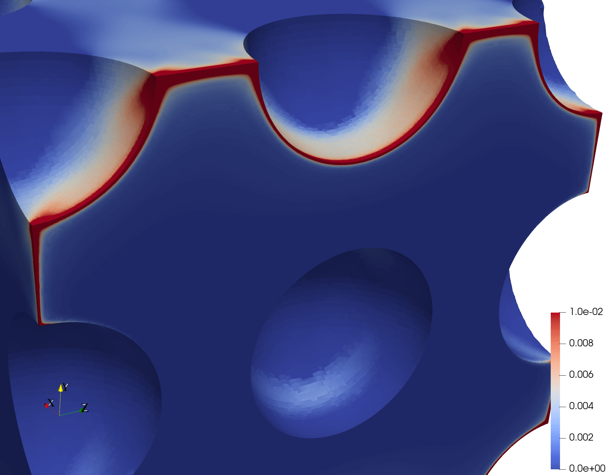
b

Figure 10. 3D Cantilever beam test: Final stage: (A) FE mesh. (B) J2 Plasticity internal variable $\alpha$.

In Fig. 11 and Table 3 we report the same concepts as its counterparts Fig. 8 and Table 2, resp., for the experiment at hand. Overall, very similar conclusions to the ones in the previous section, with some subtle differences, can be extracted from these results. First, in Fig. 11, we can observe larger intervals in-between mesh adaptations than those observed in the previous section, and thus even more reduced computational times compared to other heuristic, non-error-driven strategies. Second, in Table 3 we can also observe a high variability in the number of nonlinear iterations with load step. However, this time, there is a clear steady increase in this number with increasing load.

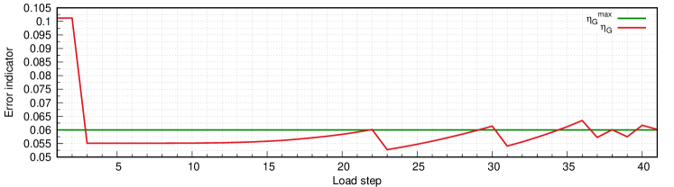
Figure 11. 3D Cantilever beam test: Evolution of $\eta_{G}$.

Concept   \  load step	1-2	3-22	23-30	31-36	37-38	39-40	41
Free DOFs [M]	0.592	1.637	2.425	3.553	5.258	7.840	11.69
Total background mesh cells [M]	0.249	0.722	1.050	1.537	2.255	3.322	4.907
Active cells (% Total cells)	82.17	90.08	91.67	92.88	94.11	94.94	95.56
Accumulated adaptivity cycles	0	3	4	5	6	7	8
Average nonlinear iters. per load step	1	5	7	10	16	26	33

Table 3. Evolution of AMR cycles, size of the problem and (average) nonlinear iterations (3D Cantilever test).

We perform a strong scalability study of Alg. 1 when applied to the problem described above on the NCI-Gadi supercomputer [41]; see Section 6.1. The challenge resides in the fact that, as seen in Fig. 10, localization, and thus refinement along the domain, is not aligned with the initial uniform distribution of load (note that we start the loading process with a uniform mesh). As a consequence, during a load stepping adaptive simulation, the computational load of the different cores will become rapidly highly unbalanced if one does not dynamically reshuffle the mesh and associated fields among them during the simulation. Recall that, in Alg. 1, this is triggered in line 1. In order to illustrate this, in Fig. 12a and 12b we show the distribution of load (active cells) among 288 cores in the initial and final load steps. As expected, the initial distribution of load is uniform, with similarly shaped subdomains. However, the final distribution of load is far from uniform, with a subdomains density (number of subdomains per unit volume) much higher close to the clamped face. Indeed, as expected, the cells which cover the $x\geq L/2$ half of the beam are owned by a very small portion of subdomains as effect of dynamic load balancing. We note that, as there is communication overhead involved in the repartitioning of data, it is thus interesting to study whether for the problem at hand this overhead is outweighed by the gains derived from a better distribution of computational load.

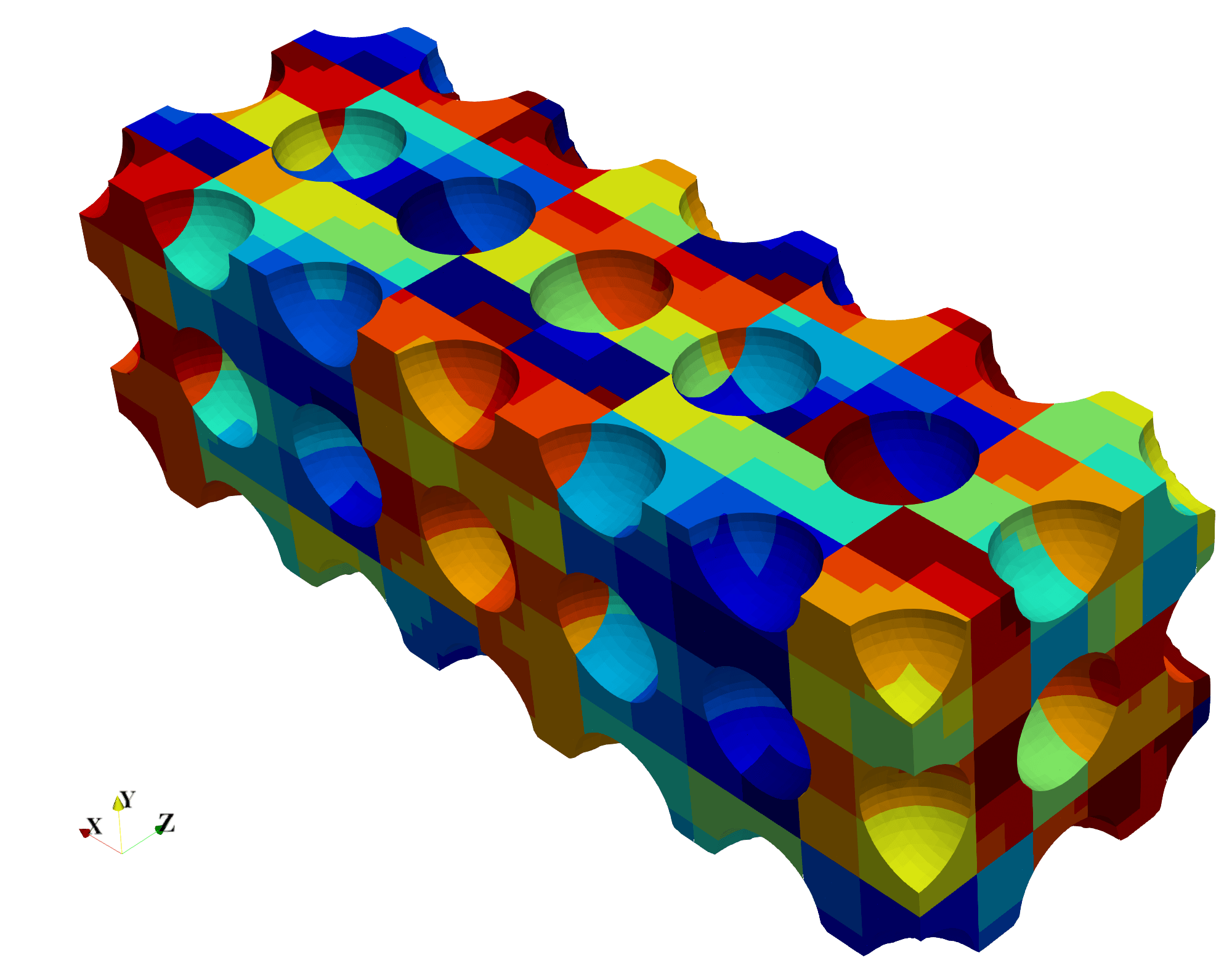
a

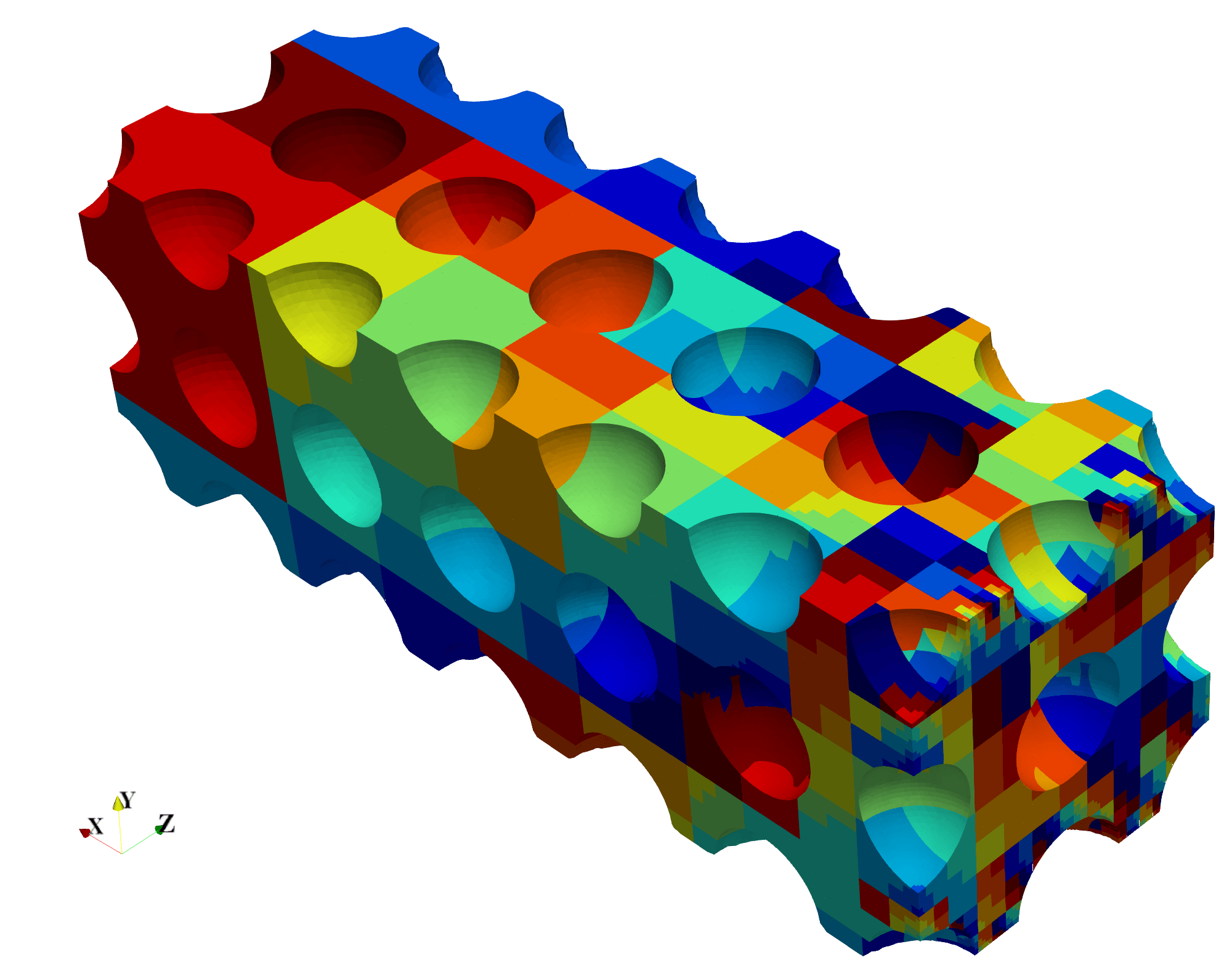
b

Figure 12. 3D Cantilever beam: (A) initial and (B) final distribution of active cells among cores.

The results of the strong scalability test are given in Table 4. We recall that, as shown in Table 3, the size of the discrete problem in the last load step is around 11.7M DOFs. The simulation consumes, at its maximum, around 86% of the total amount of memory available when deployed on 4 nodes (192 cores) on the NCI-Gadi supercomputer; see Sect. 6.1. The wall clock times in the table reported include the full load increment simulation, end-to-end, as reported by the Job Queuing System. Thus, this is the true time that the user experiences when using the software. The value given in the row labeled as EST (Extrapolated Sequential Time) is computed as the actual time measured with 192 cores, multiplied by a factor of 192, and can be considered as an estimation of the sequential execution time under ideal conditions (linear speed-up). In practice, one may expect it to be even higher (as there is typically loss of parallel efficiency to some extent). Note that we had to estimate this time as the problem at hand does not fit into a single node.

P	Wall clock Time	$S_{p}$	$E_{p}$	#DOFs per core
EST	4936h 32m 00s	—	—	11,687,673
192	25h 42m 40s	—	—	60,873
384	10h 46m 22s	2.390	1.190	30,436
768	5h 24m 15s	4.760	1.190	15,218
1,536	2h 58m 15s	8.650	1.080	7,609
3,072	1h 49m 14s	14.120	0.880	3,804

Table 4. 3D Cantilever beam - strong scalability test. #DOFs per core is computed as the total number of DOFs divided by the number of cores ($p$). Simulation ends after 41 load steps.

The column labeled as $S_{p}$ (speed-up) in Table 4 is defined as the ratio between the parallel execution time on $192$ cores (reference time), referred to as $t_{192}$, and the parallel execution time on $p$ cores, i.e. $S_{p}=t_{192}/t_{p}$. The column labeled as $E_{p}$ (parallel efficiency), is defined as $E_{P}=S_{p}/k$, with $k=p/192$. Clearly, the most salient property of the framework, as can be shown in Table 4, is its ability to efficiently reduce execution times with increasing number of cores despite the localization challenge. A closer inspection of the load balance achieved reveals that the relative difference among the subdomains with the maximum and minimum number of DOFs stays well below 1% during the whole simulation versus differences of more than 100% when dynamic load balance is deactivated. By exploiting parallel resources, the execution time is reduced by a factor of $14.120$ when $3072$ cores are used. For practical purposes, these speed-ups reflect a reduction of the execution time in industrial simulations from months (as in the EST) to less than a couple of hours when $3$K cores are used. The loss of parallel performance with $p$ is associated to parallelism related overheads; in this case, more computationally intensive simulations, involving larger loads per core, are required to exploit the computational resources more efficiently.

In order to gain more insight on the results in Table 4, we profiled the execution of the framework for $P=192$ cores. It turns out that the bulk of the computation is concentrated in the nonlinear solver, which amounts to 75% of the total computation time (i.e. aggregated across all load steps). Out of this 75%, the computation of the residual, Jacobian, and preconditioned iterative solution of linear systems concentrate 32%, 14%, 28%, resp., of the total computation time. This is followed by the computation of error estimators, which concentrates 9% of the total computation time. Finally, the updates of global FE spaces required after adaptation and redistribution amounts to 3%, and those related to the background mesh, embedded domain boundary intersection, and setting up the aggregates, to 0.5%. The timings in Table 4, both in magnitude, and the rate at which they decrease with $P$ (note that the computation of the residual and Jacobian are highly parallel stages), can be justified, among others, by the number of nonlinear iterations required to achieve convergence; see results in Table 3. Besides, the acceleration caused by sticking into a balanced computational load largely outweighs the extra overhead associated to dynamic load balancing.

7. Conclusions

This work extends the $h$-AgFEM to the context of nonlinear solid mechanics problems. To the best of the authors’ knowledge, this is the first fully parallel distributed-memory unfitted $h$-adaptive FE framework robust with respect to small cut cells that solves nonlinear solid mechanics problems. It is grounded on five main building blocks: 1) unfitted formulations (using aggregation techniques) that are robust irrespective of the cut locations, 2) a strategy to deal with history variables of any tensorial order provided by the constitutive model in combination with aggregated spaces, 3) an algorithm for the solution of nonlinear problems based on the Newton-Raphson method, endowed with optimization strategies to improve the performance of the nonlinear solver in highly nonlinear scenarios, 4) an algorithm to solve the nonlinear problem incrementally that includes hierarchical AMR to provide an adapted mesh able to capture the evolution of inelastic behavior and 5) a distributed-memory implementation that relies on parallel linear solvers and octree engines with dynamic load-balancing at each adaptive step.

The proposed framework has been extensively tested with a large set of experiments for both irreducible and mixed (u/p) formulations that include incompressible materials. These experiments reveal good accuracy in terms of error convergence when comparing the numerical solution with the analytical one (when provided) and show that the onset of nonlinearity in unfitted boundaries is properly captured; this becomes a crucial issue in tests involving complex geometries where the inelastic behavior takes place in weak regions of the physical domain. These experiments not only have verified efficiency and robustness of the framework, but also revealed the sensitivity of the AMR strategy to capture localized nonlinear regions as consequence of complex load scenarios. The scalability properties of the framework have also been analyzed.

We have applied this framework to more complex periodic structures in order to show how the framework can efficiently deal with these geometries, avoiding the need to generate very costly body-fitted meshes and graph partitioners. Body-fitted meshing is a computational bottleneck that requires human intervention and prevents an automatic geometry-to-solution workflow. On the contrary, the framework proposed in this work is fully automatic and highly scalable. This fact enables, e.g. robust optimization of structures or uncertainty quantification of structures with random domains [48]. This framework is particularly relevant in AM, in order to virtually certify and optimize mesoscale lattice structures or to quantify the effect of geometrical irregularities, or to handle growing geometries in AM process simulations [3].

References

- Echeta et al. [2020] I. Echeta, X. Feng, B. Dutton, R. Leach, and S. Piano. Review of defects in lattice structures manufactured by powder bed fusion. International Journal of Advanced Manufacturing Technology, 106(5-6):2649–2668, 2020. doi:10.1007/s00170-019-04753-4.
- Plocher and Panesar [2019] J. Plocher and A. Panesar. Review on design and structural optimisation in additive manufacturing: Towards next-generation lightweight structures, 2019.
- Neiva et al. [2019] E. Neiva, S. Badia, A. F. Martin, and M. Chiumenti. A scalable parallel finite element framework for growing geometries. application to metal additive manufacturing. International Journal for Numerical Methods in Engineering, 119(11):1098–1125, 2019. doi:10.1002/nme.6085.
- Bangerth et al. [2012] W. Bangerth, C. Burstedde, T. Heister, and M. Kronbichler. Algorithms and data structures for massively parallel generic adaptive finite element codes. ACM Trans. Math. Softw., 38(2), 2012. doi:10.1145/2049673.2049678.
- Badia et al. [2020] S. Badia, A. F. Martín, E. Neiva, and F. Verdugo. A generic finite element framework on parallel tree-based adaptive meshes. SIAM Journal on Scientific Computing, 42(6):C436–C468, 2020. doi:10.1137/20M1328786.
- Burman et al. [2015] E. Burman, S. Claus, P. Hansbo, M. G. Larson, and A. Massing. Cutfem: Discretizing geometry and partial differential equations. International Journal for Numerical Methods in Engineering, 104(7):472–501, 2015. doi:10.1002/nme.4823.
- Schillinger and Ruess [2015] D. Schillinger and M. Ruess. The finite cell method: A review in the context of higher-order structural analysis of cad and image-based geometric models. Archives of Computational Methods in Engineering, 22(3):391–455, 2015. doi:10.1007/s11831-014-9115-y.
- Badia et al. [2018a] S. Badia, F. Verdugo, and A. F. Martin. The aggregated unfitted finite element method for elliptic problems. Computer Methods in Applied Mechanics and Engineering, 336:533 – 553, 2018a. doi:10.1016/j.cma.2018.03.022.
- Badia et al. [2018b] S. Badia, A. F. Martin, and F. Verdugo. Mixed aggregated finite element methods for the unfitted discretization of the stokes problem. SIAM Journal on Scientific Computing, 40(6):B1541–B1576, 2018b. doi:10.1137/18M1185624.
- Badia et al. [2021] S. Badia, A. F. Martín, E. Neiva, and F. Verdugo. The aggregated unfitted finite element method on parallel tree-based adaptive meshes. SIAM Journal on Scientific Computing, 43(3):C203–C234, 2021. doi:10.1137/20M1344512.
- Verdugo et al. [2019] F. Verdugo, A. F. Martin, and S. Badia. Distributed-memory parallelization of the aggregated unfitted finite element method. Computer Methods in Applied Mechanics and Engineering, 357:112583, 2019. doi:10.1016/j.cma.2019.112583.
- Neiva and Badia [2021] E. Neiva and S. Badia. Robust and scalable h-adaptive aggregated unfitted finite elements for interface elliptic problems. Computer Methods in Applied Mechanics and Engineering, 380:113769, 2021. doi:https://doi.org/10.1016/j.cma.2021.113769.
- Johnson and Hansbo [1992] C. Johnson and P. Hansbo. Adaptive finite element methods in computational mechanics. Computer Methods in Applied Mechanics and Engineering, 101(1):143 – 181, 1992. doi:10.1016/0045-7825(92)90020-K.
- Rannacher and Suttmeier [1999] R. Rannacher and F.-T. Suttmeier. A posteriori error estimation and mesh adaptation for finite element models in elasto-plasticity. Computer Methods in Applied Mechanics and Engineering, 176(1):333 – 361, 1999. doi:10.1016/S0045-7825(98)00344-2.
- Frohne et al. [2016] J. Frohne, T. Heister, and W. Bangerth. Efficient numerical methods for the large-scale, parallel solution of elastoplastic contact problems. International Journal for Numerical Methods in Engineering, 105(6):416–439, 2016. doi:10.1002/nme.4977.
- Ghorashi and Rabczuk [2017] S. S. Ghorashi and T. Rabczuk. Goal-oriented error estimation and mesh adaptivity in 3d elastoplasticity problems. International Journal of Fracture, 203(1):3–19, Jan 2017. doi:10.1007/s10704-016-0113-y.
- Rüberg et al. [2016] T. Rüberg, F. Cirak, and J. García Aznar. An unstructured immersed finite element method for nonlinear solid mechanics. Advanced Modeling and Simulation in Engineering Sciences, 3(1):22, 2016. doi:10.1186/s40323-016-0077-5.
- Rüberg and Aznar [2016] T. Rüberg and J. G. Aznar. Numerical simulation of solid deformation driven by creeping flow using an immersed finite element method. Advanced Modeling and Simulation in Engineering Sciences, 3(1):9, 2016. doi:10.1186/s40323-016-0061-0.
- Schillinger et al. [2013] D. Schillinger, Q. Cai, R.-P. Mundani, and E. Rank. A review of the finite cell method for nonlinear structural analysis of complex cad and image-based geometric models. In M. Bader, H.-J. Bungartz, and T. Weinzierl, editors, Advanced Computing, pages 1–23, Berlin, Heidelberg, 2013. Springer Berlin Heidelberg.
- Duster et al. [2008] A. Duster, J. Parvizian, Z. Yang, and E. Rank. The finite cell method for three-dimensional problems of solid mechanics. Computer Methods in Applied Mechanics and Engineering, 197:3768–3782, 2008. doi:10.1016/j.cma.2008.02.036.
- Hansbo et al. [2017] P. Hansbo, M. G. Larson, and K. Larsson. Cut finite element methods for linear elasticity problems. In S. P. A. Bordas, E. Burman, M. G. Larson, and M. A. Olshanskii, editors, Geometrically Unfitted Finite Element Methods and Applications, pages 25–63, Cham, 2017. Springer International Publishing.
- Balay et al. [2020] S. Balay, S. Abhyankar, M. F. Adams, J. Brown, P. Brune, K. Buschelman, L. Dalcin, A. Dener, V. Eijkhout, W. D. Gropp, D. Karpeyev, D. Kaushik, M. G. Knepley, D. A. May, L. C. McInnes, R. T. Mills, T. Munson, K. Rupp, P. Sanan, B. F. Smith, S. Zampini, H. Zhang, and H. Zhang. PETSc users manual. Technical Report ANL-95/11 - Revision 3.13, Argonne National Laboratory, 2020.
- Simo and Hughes [1998] J. Simo and T. Hughes. Computational inelasticity. Springer-Verlag, 1998.
- de Souza Neto D. Peric D. R. J. Owen [2008] E. A. de Souza Neto D. Peric D. R. J. Owen. Computational Methods for Plasticity: Theory and Applications. John Wiley & Sons, Ltd Eds., 2008. doi:10.1002/9780470694626.
- Johnson [1978] C. Johnson. On plasticity with hardening. Journal of Mathematical Analysis and Applications, 62(2):325 – 336, 1978. doi:10.1016/0022-247X(78)90129-4.
- Burman and Hansbo [2012] E. Burman and P. Hansbo. Fictitious domain finite element methods using cut elements: Ii. a stabilized nitsche method. Applied Numerical Mathematics, 62(4):328 – 341, 2012. doi:10.1016/j.apnum.2011.01.008.
- Müller et al. [2017] B. Müller, S. Krämer-Eis, F. Kummer, and M. Oberlack. A high-order discontinuous Galerkin method for compressible flows with immersed boundaries. International Journal for Numerical Methods in Engineering, 110(1):3–30, 2017. doi:10.1002/nme.5343.
- Burstedde et al. [2011] C. Burstedde, L. C. Wilcox, and O. Ghattas. p4est: Scalable Algorithms for Parallel Adaptive Mesh Refinement on Forests of Octrees. SIAM Journal on Scientific Computing, 33(3):1103–1133, 2011. doi:10.1137/100791634.
- Chin et al. [2015] E. B. Chin, J. B. Lasserre, and N. Sukumar. Numerical integration of homogeneous functions on convex and nonconvex polygons and polyhedra. Computational Mechanics, 56(6):967–981, 2015. doi:10.1007/s00466-015-1213-7.
- Badia and Verdugo [2018] S. Badia and F. Verdugo. Robust and scalable domain decomposition solvers for unfitted finite element methods. Journal of Computational and Applied Mathematics, 344:740 – 759, 2018. doi:10.1016/j.cam.2017.09.034.
- Ciarlet [1978] P. G. Ciarlet. The finite element method for elliptic problems. North-Holland Pub. Co., 1978.
- Dennis and Schnabel [1996] J. E. Dennis and R. B. Schnabel. Numerical Methods for Unconstrained Optimization and Nonlinear Equations. Society for Industrial and Applied Mathematics, 1996. doi:10.1137/1.9781611971200.
- Babuska and Rheinboldt [1978] I. Babuska and W. C. Rheinboldt. A-posteriori error estimates for the finite element method. International Journal for Numerical Methods in Engineering, 12(10):1597–1615, 1978. doi:10.1002/nme.1620121010.
- Babuska [1981] I. Babuska. A-posteriori error estimation for the finite element method. In W. Wunderlich, E. Stein, and K.-J. Bathe, editors, Nonlinear Finite Element Analysis in Structural Mechanics, pages 3–10, Berlin, Heidelberg, 1981. Springer Berlin Heidelberg.
- Kelly et al. [1983] D. W. Kelly, J. P. De S. R. Gago, O. C. Zienkiewicz, and I. Babuska. A posteriori error analysis and adaptive processes in the finite element method: Part i—error analysis. International Journal for Numerical Methods in Engineering, 19(11):1593–1619, 1983. doi:10.1002/nme.1620191103.
- Grätsch and Bathe [2005] T. Grätsch and K.-J. Bathe. A posteriori error estimation techniques in practical finite element analysis. Computers & Structures, 83(4):235 – 265, 2005. doi:10.1016/j.compstruc.2004.08.011.
- Elguedj et al. [2008] T. Elguedj, Y. Bazilevs, V. Calo, and T. Hughes. B-bar an f-bar projection methods for nearly incompressible linear and non linear elasticity and plasticity using higher order nurbs element. Comput. Method Appl. Mech. Engrg., 197, 2008.
- Simo and Taylor [1986] J. C. Simo and R. L. Taylor. A return mapping algorithm for plane stress elastoplasticity. International Journal for Numerical Methods in Engineering, 22(3):649–670, 1986. doi:10.1002/nme.1620220310.
- Tao and Leu [2016] W. Tao and M. C. Leu. Design of lattice structure for additive manufacturing. In 2016 International Symposium on Flexible Automation (ISFA), pages 325–332. IEEE, 2016. doi:10.1109/ISFA.2016.7790182.
- [40] Marenostrum-IV Web site. https://www.bsc.es/marenostrum/marenostrum. Accessed: 2020-06-22.
- [41] NCI-Gadi Web site. https://nci.org.au/our-systems/hpc-systems. Accessed: 2020-06-22.
- Badia et al. [2018] S. Badia, A. F. Martin, and J. Principe. FEMPAR: An Object-Oriented Parallel Finite Element Framework. Archives of Computational Methods in Engineering, 25(2):195–271, 2018. doi:10.1007/s11831-017-9244-1.
- Badia and Martin [2020] S. Badia and A. F. Martin. A tutorial-driven introduction to the parallel finite element library fempar v1.0.0. Computer Physics Communications, 248:107059, 2020. doi:10.1016/j.cpc.2019.107059.
- Barber et al. [1996] C. Barber, D. Dobkin, , and H. Huhdanpaa. The quickhull algorithm for convex hulls. ACM Trans. on Mathematical Software, 1996.
- Hill [1950] R. Hill. The Mathematical Theory of Plasticity. Clarendon Press., 1950.
- Gao [2003] X.-L. Gao. Elasto-plastic analysis of an internally pressurized thick-walled cylinder using a strain gradient plasticity theory. International Journal of Solids and Structures, 40(23):6445 – 6455, 2003. doi:10.1016/S0020-7683(03)00424-4.
- Kittel [2004] C. Kittel. Introduction to Solid State Physics. Wiley, 8 edition, 2004.
- Badia et al. [2021] S. Badia, J. Hampton, and J. Principe. Embedded multilevel monte carlo for uncertainty quantification in random domains. International Journal for Uncertainty Quantification, pages 119–142, 2021. doi:10.1615/Int.J.UncertaintyQuantification.2021032984.