Libra: a package for transformation of differential systems for multiloop integrals.

Abstract

We present a new package for Mathematica system, called Libra. Its purpose is to provide convenient tools for the transformation of the first-order differential systems $\partial_{i}\boldsymbol{j}=M_{i}\boldsymbol{j}$ for one or several variables. In particular, Libra is designed for the reduction to $\epsilon$-form of the differential systems which appear in multiloop calculations. The package also contains some tools for the construction of general solution: both via perturbative expansion of path-ordered exponent and via generalized power series expansion near regular singular points. Libra also has tools to determine the minimal list of coefficients in the asymptotics of the original master integrals, sufficient for fixing the boundary conditions.

PROGRAM SUMMARY

Program title: Libra
CPC Library link to program files: (to be added by Technical Editor)
Developer’s respository link: (if available)
Code Ocean capsule: (to be added by Technical Editor)
Licensing provisions(please choose one): GPLv3
Programming language: Wolfram Mathematica
Nature of problem:
Transformation of the first-order linear differential systems with respect to one or several variables: reduction to fuchsian form, to $\epsilon$-form, formal solution in terms of the Goncharov’s polylogarithms and in terms of generalized power series.
Solution method:
Algorithms described in Refs. [1, 2], and [3, Section E.8].

1 Introduction

Modern multiloop calculations essentially rely on the differential equations method. Within this approach, the integration-by-part (IBP) reduction is used to reduce all requred integrals to a finite set of master integrals and to construct the first-order differential systems for the latter. The possibility to find analytic solutions of these systems essentially relies on their reduction to some kind of canonical form. This may include, for example, the elimination of spurious singularities, reduction to local/global Fuchsian form, variable change and switching to/from one higher-order differential equation. Given high complexity of the differential systems which emerge in multiloop calculations, one can not avoid using computers for the reduction.

The present paper introduces a new package for Mathematica system, called Libra. Its purpose is to provide convenient tools for the transformation of the first-order differential systems. The package also contains some tools for the construction of general solution: both via perturbative expansion of path-ordered exponent and via generalized power series expansion near regular singular points. Libra also can help the user to determine the minimal list of coefficients in the asymptotics of the original master integrals near a singular point. Calculating the coefficients from this list is sufficient for fixing the boundary conditions.

One of the most important tasks that Libra can be relied on is the reducing of the differential equations to $\epsilon$-form [Henn2013, 1]. In the next Section we review the corresponding reduction algorithm as presented in Refs. [1, 2, 3]. Note that this algorithm has been implemented in two publicly available codes, epsilon, Ref. [Prausa2017a], and Fuchsia, Ref. [Gituliar2017]. However, we believe that Libra will still be appreciated by the community due to its rich functionality and also high computational power. In this context, we note that Libra has been already used in several bleeding-edge multiloop computations, see, e.g., Refs. [Lee:2019zop, Grozin:2020jvt]. We describe the Libra package in Section 3, where one can find two examples of Libra usage.

The last, but not the least, although inspired by the multiloop applications, Libra package is quite universal and can be used in other research fields, which require manipulations with the first-order differential systems of the form $\frac{\partial}{\partial x_{i}}\boldsymbol{j}=M_{i}(\boldsymbol{x})\boldsymbol{j}$. In particular, these systems appear in algebraic geometry when considering Gauss-Manin connection.

2 Reduction to $\epsilon$-form

In the present section we shortly review the algorithm presented in Refs. [1, 2, 3]. We skip the description of IBP reduction method, Refs. [Tkachov1981, ChetTka1981], which is essential to obtain the differential equations for master integrals, [Kotikov1991b, Remiddi1997]. We start from the differential system of the form

$$\frac{\partial}{\partial x_{i}}\boldsymbol{j}=M_{i}\left(\boldsymbol{x},\epsilon\right)\boldsymbol{j}\qquad(i=1,\ldots,N).$$ (1)

Here $\boldsymbol{j}=(j_{1},\ldots,j_{n})^{\intercal}$ is a column of unknown functions, $\boldsymbol{x}=(x_{1},\ldots x_{N})$ are the variables, and $\epsilon$ is a parameter. For typical multiloop calculation setup, these are the “Laporta” master integrals, the kinematic invariants, and the dimensional regularization parameter, respectively. The matrices $M_{i}$ in the right-hand side rationally depend on $\boldsymbol{x}$ and $\epsilon$. The observation made in Ref. [Henn2013] is that by a proper choice of new functions $\boldsymbol{J}$ the differential system can often be cast in the form where the dependence on $\epsilon$ is factorized in the right-hand side,

$$\frac{\partial}{\partial x_{i}}\boldsymbol{J}=\epsilon S_{i}\left(\boldsymbol{x}\right)\boldsymbol{J}\qquad(i=1,\ldots,N).$$ (2)

In what follows we will refer to this form as $\epsilon$-form. Note that the integrability conditions applied to the system (2) imply that $M=\sum_{i}dx_{i}S_{i}(\boldsymbol{x})$ is an exact 1-form (total differential) [Henn2013].

The advantage of the differential system in $\epsilon$-form is that its general solution

$$U=\operatorname{Pexp}\left[\epsilon\int d\boldsymbol{x}\cdot\boldsymbol{S}\right]$$ (3)

can be readily expanded in $\epsilon$-series in terms of iterated integrals. In particular, for rational matrices $S_{i}$ these integrals are nothing but the multiple polylogarithms [Goncharov1998].

Therefore, a natural question arises: given the differential system (1) is it possible and how to find the transformation of functions $\boldsymbol{j}=T\boldsymbol{J}$, such that the new functions $\boldsymbol{J}$ satisfy the differential system (2)? Let us remark that, when answering to this question, it is important to restrict the class of transformations we want to consider. Otherwise, we can always pass to trivial system $d\boldsymbol{J}=0$ by means of the formal transformation $T=\operatorname{Pexp}[\int d\boldsymbol{x}\cdot\boldsymbol{M}]=\operatorname{Pexp}[\int\sum_{i}dx_{i}M_{i}]$. Our base case will be the class of transformations rational in both $\boldsymbol{x}$ and $\epsilon$. At some point we will also consider the extension of this class to the transformations rational in some notations $\boldsymbol{y}$ algebraically related to the original variables via $x_{i}=f_{i}(\boldsymbol{y})$ with $f_{i}$ being the rational functions.

An algorithm of the reduction of a univariate differential system to $\epsilon$-form has been suggested in Ref. [1]. Later on, a strict criterion of irreducibility has been obtained in Ref. [2]. Also, in the same paper it was explained how to use the algorithm for multivariate setup. We will present now a basis-independent variant of this algorithm, partly described in Ref. [3, Section E.8].

2.1 Conventions and notations

Note that the transformation of functions $\boldsymbol{j}=T\tilde{\boldsymbol{j}}$ is understood below as the transformation of matrices in the right-hand side of the differential system (1):

$$M_{i}\to\widetilde{M}_{i}=T^{-1}\left[M_{i}\,T-\frac{\partial}{\partial x_{i}}T\right].$$ (4)

As explained in Ref. [2], the problem of reduction to $\epsilon$-form of the systems in several variables is effectively reduced to that of the system in one variable. One should simply proceed on one-by-one basis, reducing first the system in the first variable, then in the second variable, etc. The only restrictions are that the transformations considered for each successive variable should not depend on the previous variables. These restrictions seem to be easily fulfilled in every specific example (see, in particular, example 5 in Tutorial1.nb notebook attached to the distribution). Therefore, from now on we consider the differential equation in one variable.

$$\partial_{x}\boldsymbol{j}=M\boldsymbol{j}.$$ (5)

Let us remind some facts from linear algebra and give a few useful definitions. First, since we are aimed at a basis-independent treatment, we find it convenient to use a mixed terminology, coming partly from the operator language and partly from the matrix language. In particular, we have the dictionary presented in Table 1.

Operator term		Matrix term
linear operator $L$	$\leftrightarrow$	$n\times n$ matrix $L$
vector $\boldsymbol{u}$	$\leftrightarrow$	column $\boldsymbol{u}=(u_{1},\ldots,u_{n})^{\intercal}$
covector $\boldsymbol{v}^{\intercal}$	$\leftrightarrow$	row $\boldsymbol{v}^{\intercal}=(v_{1},\ldots,v_{n})$
$\ker L$	$\leftrightarrow$	$\{\boldsymbol{u},\,L\boldsymbol{u}=0\}$
$\operatorname{coker}L$	$\leftrightarrow$	$\{\boldsymbol{v}^{\intercal},\,\boldsymbol{v}^{\intercal}L=0\}$
$\operatorname{Im}L$	$\leftrightarrow$	$\{\boldsymbol{u},\,\exists\tilde{\boldsymbol{u}}:L\tilde{\boldsymbol{u}}=\boldsymbol{u}\}$
$\operatorname{coIm}L$	$\leftrightarrow$	$\{\boldsymbol{v}^{\intercal},\,\exists\tilde{\boldsymbol{v}}^{\intercal}:\tilde{\boldsymbol{v}}^{\intercal}L=\boldsymbol{v}^{\intercal}\}$

Table 1: Translation dictionary between the operator and matrix languages.

Moreover, we find it convenient to identify the $k$-dimensional linear subspace (or simply $k$-subspace) $\mathcal{U}$ with the $n\times k$ matrix whose columns form some basis of this subspace. Although this matrix is not uniquely defined, nevertheless, every expression below that contains this matrix will be independent on the specific choice of the basis, so we denote this matrix also as $\mathcal{U}$. For example, the statement $\mathcal{U}\subset\ker L$ is equivalent to $L\mathcal{U}=0$. In what follows, the invariant subspaces of operators will appear. Within our mixed language the wording “$\mathcal{U}$ is invariant subspace of $L$” is equivalent to “$\exists$ matrix $C$ such that $L\mathcal{U}=\mathcal{U}C$”.

Also, we will refer to the element $\boldsymbol{v}^{\intercal}$ and subspace $\mathcal{V}^{\intercal}$ in the dual space as right vector and right subspace, as opposed to the left vector $\boldsymbol{u}$ and left subspace $\mathcal{U}$ for the original space. Note that the matrix, corresponding to $k$-dimensional right subspace $\mathcal{V}^{\intercal}$ has dimension $k\times n$ (rather than $n\times k$) which should be easy to memorize thanks to $\bullet^{\intercal}$ notation.

Finally, let us fix our notations for describing the properties of the differential system (5) in the vicinity of some point $x_{0}$. Let $M(x)$ have the following series expansion at $x=x_{0}\neq\infty$:

$$M(x)=\sum_{k=-r-1}^{\infty}M_{k}\cdot(x-x_{0})^{k}\,,$$ (6)

where $M_{-r-1}\neq 0$. Then we say that $\max(r,0)$ is a Poincare rank at $x=x_{0}$ and $M_{-1}$ is a matrix residue at $x=x_{0}$. If $r\geqslant 0$ ($r<0$), we say that $x_{0}$ is a singular point (regular point). Similarly, for the expansion near $x=\infty$,

$$M(x)=\sum_{k=-r+1}^{\infty}M_{k}\cdot x^{-k}\,,$$ (7)

we say that $\max(r,0)$ is a Poincare rank at $x=\infty$ and $-M_{1}$ is a matrix residue at $x=\infty$ (note the minus sign). If $r\geqslant 0$ ($r<0$), we say that $\infty$ is a singular point (regular point).

2.2 Projector and balance transformation

As is well-known, the projector operator $P=P^{2}$ is totally defined by its image and kernel, or, equivalently, by its image and co-image, $\mathcal{V}^{\intercal}=\operatorname{coIm}P$ and $\mathcal{U}=\operatorname{Im}P$. Given the left subspace $\mathcal{V}^{\intercal}$ and the right subspace $\mathcal{U}$ of equal dimension $k$, one can construct a projector

$$P=P(\mathcal{U},\mathcal{V}^{\intercal})=\mathcal{U}(\mathcal{V}^{\intercal}\mathcal{U})^{-1}\mathcal{V}^{\intercal}\,.$$ (8)

This is true unless the $k\times k$ matrix $\mathcal{V}^{\intercal}\mathcal{U}$ is not invertible. Note that the matrix in the right-hand side of Eq. (8) is defined uniquely despite the freedom of choice of $\mathcal{U}$ and $\mathcal{V}^{\intercal}$. The properties $P^{2}=P,\ \operatorname{Im}P=\mathcal{U},\ \operatorname{coIm}P=\mathcal{V}^{\intercal}$ can be readily verified.

Given a projector $P$, we define $P$-balance transformation between two finite points $x_{1}$ and $x_{2}$ as

$$B(P,x_{1},x_{2}|x)=\overline{P}+\frac{x-x_{2}}{x-x_{1}}P,$$ (9)

where $\overline{P}=1-P$. Similarly, we define

$$B(P,x_{1},\infty|x)=\overline{P}+\frac{1}{x-x_{1}}P,\quad B(P,\infty,x_{2}|x)=\overline{P}+(x-x_{2})P.$$ (10)

When $P=P(\mathcal{U},\mathcal{V}^{\intercal})$ we also write $B(\mathcal{U},\mathcal{V}^{\intercal}|x_{1},x_{2}|x)=B(P(\mathcal{U},\mathcal{V}^{\intercal}),x_{1},x_{2}|x)$.

The balance transformation may change the Poincare rank of $M$ and the eigenvalues of the matrix residue in two points, $x=x_{1}$ and $x=x_{2}$, at most.

We will call the balance transformation $B(\mathcal{U},\mathcal{V}^{\intercal}|x_{1},x_{2}|x)$ an $x_{1}$-adjusted ($x_{2}$-adjusted) if it does not increase the Poincare rank of the system at $x=x_{1}$ (at $x=x_{1}$). It is easy to prove that $B(\mathcal{U},\mathcal{V}^{\intercal}|x_{1},x_{2}|x)$ is $x_{1}$-adjusted iff $x_{1}$ is a singular point and $\mathcal{U}$ is a left invariant subspace of the leading series expansion coefficient of $M(x)$ near $x=x_{1}$. Similarly, $B(\mathcal{U},\mathcal{V}^{\intercal}|x_{1},x_{2}|x)$ is $x_{2}$-adjusted iff $x_{2}$ is a singular point and $\mathcal{V}^{\intercal}$ is a right invariant subspace of the leading series expansion coefficient near $x=x_{2}$.

In what follows we will always use the balances that are adjusted in both points, unless otherwise stated.

2.3 Reducing Poincare rank and shifting eigenvalues of matrix residues

Let us consider now the point of positive Poincare rank, e.g., let it be $x=0$. So, we have ($r>0$)

$$M(x)=\sum_{k=-r-1}^{\infty}M_{k}\cdot x^{k}=\frac{A_{0}}{x^{r+1}}+\frac{A_{1}}{x^{r}}+\ldots\,.$$ (11)

We want to find the adjusted balance transformation to strictly reduce the matrix rank of $A_{0}=M_{-r-1}$. Let us search for the balance having zero as the first singular point, $B(\mathcal{U},\mathcal{V}^{\intercal}|0,x_{2}|x)$. As it is described in Ref. [3, Section E.8], it suffices to find $\mathcal{U}$ with the following properties:

$$\mathrm{I.}\quad A_{0}\mathcal{U}=0,\qquad\mathrm{II.}\quad A_{1}\mathcal{U}\subseteq\operatorname{Im}A_{0}+\mathcal{U},\qquad\mathrm{III.}\quad\mathcal{U}\cap\operatorname{Im}A_{0}>\{0\}.$$ (12)

A necessary and sufficient criterion of the existence of such a $\mathcal{U}$ is [3, Section E.8]

$$\dim\ker\mathcal{A}>\dim\ker A_{0}\,,$$

where

$$\mathcal{A}=\begin{pmatrix}A_{0}&A_{1}-\lambda\\ 0&A_{0}\end{pmatrix}\,.$$ (13)

This condition simply states that the number of null eigenvectors of the matrix $\mathcal{A}$ should be greater than that of $A_{0}$. Let us note that if $\boldsymbol{u}$ is a null eigenvector of $A_{0}$ then $\boldsymbol{u}\choose\boldsymbol{0}$ is that of $\mathcal{A}$, and vice versa. Therefore, the criterion (2.3) states that there must be at least one null eigenvector of $\mathcal{A}$ of the form $\boldsymbol{w}(\lambda)\choose\boldsymbol{u}(\lambda)$ with $\boldsymbol{u}(\lambda)\neq 0$. The null eigenvectors can be found routinely and their components are, in general, the rational functions of $\lambda$. As one can always get rid of common denominator, we can assume that these components are polynomials in $\lambda$ and

$$\boldsymbol{u}(\lambda)=\boldsymbol{u}_{0}+\boldsymbol{u}_{1}\lambda+\ldots\boldsymbol{u}_{k}\lambda^{k}$$ (14)

Now, we can easily check that $\mathcal{U}=\mathrm{span}(\boldsymbol{u}_{0},\ldots,\boldsymbol{u}_{k})$ satisfies conditions (12).

If we are looking for the balance $B(\mathcal{U},\mathcal{V}^{\intercal}|x_{1},0|x)$, having zero as the second singular point, we have some requirements for $\mathcal{V}^{\intercal}$. To construct $\mathcal{V}^{\intercal}$ with the required properties, we find the right null eigenvector $(\boldsymbol{v}^{\intercal}(\lambda),\boldsymbol{w}^{\intercal}(\lambda))$ of $\mathcal{A}$, such that

$$v^{\intercal}(\lambda)=\boldsymbol{v}^{\intercal}_{0}+\boldsymbol{v}^{\intercal}_{1}\lambda+\ldots\boldsymbol{v}^{\intercal}_{k}\lambda^{k}\neq\boldsymbol{0}\,.$$ (15)

Then we put $\mathcal{V}^{\intercal}=\mathrm{span}(\boldsymbol{v}^{\intercal}_{0},\ldots,\boldsymbol{v}^{\intercal}_{k})$.

Now, let the system have zero Poincare rank (Fuchsian singularity) at $x=0$:

$$M(x)=\sum_{k=-1}^{\infty}M_{k}\cdot x^{k}=\frac{A_{0}}{x}+A_{1}+\ldots\,.$$ (16)

Let us consider the balance $B(\mathcal{U},\mathcal{V}^{\intercal}|0,x_{2}|x)$, where $\mathcal{U}$ is the left invariant subspace of $A_{0}$. In a suitable basis the matrices $P=P(\mathcal{U},\mathcal{V}^{\intercal})$, $A_{0}$, and $A_{1}$ have the following block forms

$$P=\begin{pmatrix}1&0\\ 0&0\end{pmatrix}\,,\quad A_{0}=\begin{pmatrix}B_{1}&B_{2}\\ 0&B_{3}\end{pmatrix}\,,\quad A_{1}=\begin{pmatrix}B_{4}&B_{5}\\ B_{6}&B_{7}\end{pmatrix}$$ (17)

Then the expansion of the transformed matrix starts from $\frac{\tilde{A}_{0}}{x}$ where

$$\tilde{A}_{0}=\overline{P}A_{0}+(A_{0}+1)P+\overline{P}A_{1}P=\begin{pmatrix}B_{1}+1&0\\ B_{6}&B_{3}\end{pmatrix}$$ (18)

Thus, the eigenvalues, corresponding to $\mathcal{U}$ are shifted by $+1$.

If we instead apply the balance $B(\mathcal{U},\mathcal{V}^{\intercal}|x_{1},0|x)$ with $\mathcal{V}^{\intercal}$ being the right-invariant subspace of $A_{0}$, the corresponding eigenvalues are shifted by $-1$.

Let us summarize the content of this subsection. We have shown that the balance transformation $B(\mathcal{U},\mathcal{V}^{\intercal}|x_{1},x_{2}|x)$ can be used to reduce the Poincare rank and to shift the eigenvalues at Fuchsian singular points. Moreover, the discussed properties of the transformation at $x=x_{1}$ depend only on $\mathcal{U}$, while those at $x=x_{2}$ depend on $\mathcal{V}^{\intercal}$, so these two subspaces can be constructed almost independently. The only requirement that simultaneously involves $\mathcal{U}$ and $\mathcal{V}^{\intercal}$ is that $\mathcal{V}^{\intercal}\mathcal{U}$ should be a square invertible matrix.

2.4 Factoring out $\epsilon$

Suppose now that we have been able to find the global Fuchsian form with all eigenvalues of matrix residues proportional to $\epsilon$. It means that the matrix in the right-hand side now has the form

$$M(x,\epsilon)=\sum_{k}\frac{M_{k}(\epsilon)}{x-x_{k}}$$ (19)

and all eigenvalues of all $M_{k}(\epsilon)$ are proportional to $\epsilon$. Then, thanks to Proposition 1 from Ref. [2], if $\epsilon$-form exists, it can be obtained by some transformation $T(\epsilon)$ independent of $x$. In order to find this transformation, we solve the linear system of equations [1]

$$\frac{M_{k}(\epsilon)}{\epsilon}T(\epsilon,\mu)=T(\epsilon,\mu)\frac{M_{k}(\mu)}{\mu}$$ (20)

with respect to the matrix elements of $T(\epsilon,\mu)$. Note that from Eq. (20) it follows that

$$\frac{M(x,\epsilon)}{\epsilon}T(\epsilon,\mu)=T(\epsilon,\mu)\frac{M(x,\mu)}{\mu}$$ (21)

If this system has the invertible solution for some $\mu$, the transformation $T(\epsilon)=T(\epsilon,\mu)$ reduces our system to $\epsilon$-form, which becomes obvious once we multiply (21) by $\epsilon\,T^{-1}$ from the left. We note here, that in real-life examples $x_{k}$ might be complicated algebraic numbers not even expressible in terms of radicals. Then, instead of solving the system (20), we might use sufficient number of rational sampling points $x=a_{1},\ldots a_{m}$ and solve the linear system

$$\frac{M(a_{k},\epsilon)}{\epsilon}T(\epsilon,\mu)=T(\epsilon,\mu)\frac{M(a_{k},\mu)}{\mu},\quad(k=1,\ldots,m),$$ (22)

which has the advantage of having rational coefficients. Besides, this method can be easily generalized to multivariate case.

2.5 Using the block-triangular form

The real-life examples of the differential systems which one might meet in the contemporary multiloop calculations may include several hundreds of equations. It is neither possible nor necessary to reduce such systems as a whole. Rather, one should use the block-triangular structure of the systems as already described in Ref. [1]. Here we will only note that reducing the powers of irreducible denominators in the off-diagonal elements can be done without factorizing them into linear factors. Suppose, e.g., that we have in our system some denominator

$$d(x)=d_{0}+d_{1}x+\ldots+d_{n}x^{n}$$

being the irreducible polynomial of $n$-th degree. Using the same notations as in Eq. (7.1) of Ref. [1] we have the differential systems

$$d(x)\partial_{x}\boldsymbol{J}_{1} =\epsilon A(x)\boldsymbol{J}_{1}+\frac{B(x,\epsilon)}{d(x)^{r}}\boldsymbol{J}_{2}+\ldots,$$

$$d(x)\partial_{x}\boldsymbol{J}_{2} =\epsilon C(x)\boldsymbol{J}_{2}+\ldots,$$ (23)

Here $r$ is the Poincare rank of the system at any zero of $d(x)$ and the dots denote the terms which are either less singular at zeros of $d(x)$ or correspond to the contributions of lower sectors. By assumption $r>0$. Note that we may restrict ourselves to the case when the matrices $A(x)$, $B(x,\epsilon)$ and $C(x)$ have entries which are polynomials of, at most, $(n-1)$-th degree. Indeed, suppose that some entry of $A$, $B$, or $C$ has the form $\frac{p(x)}{q(x)}$, where $p(x)$ and $q(x)$ are coprime polynomials and $q(x)$ is coprime with $d(x)$. Then we use a well-known technique to reduce the rational function $\frac{p(x)}{q(x)}$ with respect to $d(x)$. Thus, we have

$$\frac{p(x)}{q(x)}=r(x)+d(x)\frac{s(x)}{q(x)}\,,$$ (24)

where $r(x)$ and $s(x)$ are some polynomials, and $r(x)$ has degree $n-1$ at most. Note that we basically have to treat $x$ as algebraic extension of $\mathbb{Q}$, defined by the equation $d(x)=0$. In particular, we use the extended Euclidean algorithm to invert $q(x)$. The corresponding procedures are implemented in many computer algebra systems, e.g., in Fermat [lewis2008computer], but, unfortunately, not in Mathematica. We have implemented the required algorithms in Libra, so that $r(x)$ can be obtained by the command QuolyMod[$p(x)/q(x)$,$x\to d(x)$’missing. In what follows we will adopt the notation

$$\frac{p(x)}{q(x)}=r(x)\quad(\mathrm{mod}\ d).$$ (25)

Then we can replace $\frac{p(x)}{q(x)}$ with $r(x)$ and move the term $d(x)\frac{s(x)}{q(x)}$ to the part hidden with dots in Eq. (2.5). So, we assume that

$$A(x)=\sum_{k=0}^{n-1}A_{k}x^{k},\quad B(x,\epsilon)=\sum_{k=0}^{n-1}B_{k}(\epsilon)x^{k},\quad C(x)=\sum_{k=0}^{n-1}C_{k}x^{k}.$$

Then we make the substitution

$$\boldsymbol{J}_{1}=\tilde{\boldsymbol{J}}_{1}+d(x)^{-r}D\boldsymbol{J}_{2},$$ (26)

where $D=D(x,\epsilon)=\sum_{k=0}^{n-1}D_{k}(\epsilon)x^{k}$ is some matrix. Collecting the most singular terms, containing $d^{-r}$, we obtain

$$d(x)\partial_{x}\tilde{\boldsymbol{J}}_{1}=\epsilon A\tilde{\boldsymbol{J}}_{1}+\left[rd^{\prime}D+\epsilon(AD-DC)+B\right]d(x)^{-r}J_{2}+\ldots$$ (27)

Then we have the equation

$$d^{\prime}D+\frac{\epsilon}{r}(AD-DC)=-\frac{B}{r}\quad(\mathrm{mod}\ d)$$ (28)

Since $d$ is irreducible, $d^{\prime}$ is coprime with $d$, so we can divide the equation by $d^{\prime}$,

$$D+\frac{\epsilon}{r}\frac{AD-DC}{d^{\prime}}=-\frac{B}{rd^{\prime}}\quad(\mathrm{mod}\ d),$$ (29)

and think of $\frac{AD-DC}{d^{\prime}}$ and $\frac{B}{rd^{\prime}}$ as some polynomial matrices of degree $n-1$. Then this equation necessarily has a solution as the linear operator acting on $D$ in the right-hand side is close to unity for sufficiently small $\epsilon$ and, thus, is invertible for generic $\epsilon$.

3 Libra package

3.1 Package installation

The Libra package can be retrieved from its web site rnlee.bitbucket.io/Libra/ or directly from the bitbucket repository bitbucket.org/rnlee/libra/. The installation amounts to unpacking the archive into any desired directory and to creating a shortcut file init.m in Mathematica $UserBaseDirectory. To automatize the creation of the shortcut, the Mathematica script makeShortcut.m should be run. More detailed instructions can be found in the INSTALL text file.

After the installation, the package is loaded with the command

• <​​<Libra`

Let us now present two examples of Libra’s usage.

3.2 Example 1: Reducing system of 5 equations

Let us consider the differential system of 5 equations with the following matrix standing in the right-hand side:

• m =

       {{(1-2*x+x^2-5*e+10*x*e-7*x^2*e+6*e^2-8*x*e^2+6*x^2*e^2)/((-1+x)*x*(1+x)*e),(-2*(-1+x))/(x^2*(1+x)),
    -2*(1-x)*(1-3*e)/(x^2*(1+x)*e),2*(1-x)/(x^2*(1+x)),2*(1-x)*(1+2*e)/(x^2*(1+x)*e)},{(1-3*e)*(1-4*e)*x/(1-x^2),
    (1+x^2-2*x*e)/((1-x^2)*x),(2*(1-5*e))/(1-x^2),-6*e/(1-x^2),0},{((1-3*e)*(1-4*e)*((1-x)^2-2*e-2*x^2*e))/(2*(1-x^2)*e),
    (-1+2*x-x^2+4*e-4*x*e+4*x^2*e)/((1-x^2)*x),(1-2*x+x^2-6*e+10*x*e-6*x^2*e+12*e^2-8*x*e^2+12*x^2*e^2)/((1-x^2)*x*e),
    (-(1-x)^2+4*e*(1-x+x^2))/((1-x^2)*x),-(1-x)*(1+2*e)*(1-3*e)/(x*(1+x)*e)},{(x*(1-3*e)*(1-4*e))/(1-x^2),-6*e/(1-x^2),
    (2*(1-5*e))/(1-x^2),(1+x^2-2*x*e)/((1-x^2)*x),0},{(-1+4*e)*(1+x+x^2-e*(5-x+5*x^2)+2e^2*(3-x+3*x^2))/((1-x^2)*(1+2*e)),
    2*e*(1+x+x^2-4*e+6*x*e-4*x^2*e)/((1-x^2)*x*(1+2*e)),-2*(1+x+x^2-e*(7+x+7*x^2)+2*e^2*(6-5*x+6*x^2))/((1-x^2)*x*(1+2*e)),
    2*e*(1+x+x^2-4*e+6*x*e-4*x^2*e)/((1-x^2)*x*(1+2*e)),2*(1+x^2-2*e+6*x*e-2*x^2*e)/((1-x^2)*x)}}/.e->\[Epsilon];

We initialize the new differential system with the command

• NewDSystem[ds1,x$\displaystyle\boldsymbol{\to}$m];

The effect of this command is that all following subsequent transformations will be attached to ds1 symbol. In particular, we can use DumpSave["ds1.m", ds1] to save our work to a file ds1.m to recover later with Get["ds1.m"]. The original matrix ’missing can be printed with ds1[x’missing. Now we are going to run the visual tool in order to find the appropriate transformation

• t=VisTransformation[ds1,x,ϵ];

After invoking this command the following window appears:

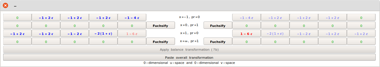
Figure 1: Visual tool for finding a (sequence of) balancing transformation(s).

This interface allows one to construct a balance transformation from the two subspaces, $\mathcal{U}$ and $\mathcal{V}^{\intercal}$, which are defined using the left and the right halves of the window, respectively. When the two subspaces are suitable for constructing the projector, i.e., have equal nonzero dimension and the matrix $\mathcal{V}^{\intercal}\mathcal{U}$ is invertible, the two lower buttons labeled by “Apply balance transformatio’missing” (below referred to as “Appl’missing” button) and “Paste overall transformatio’missing” (“Past’missing” button) turn green and enabled. When the matrix $\mathcal{V}^{\intercal}\mathcal{U}$ is not invertible, those two buttons turn red. The effect of pressing the button “Past’missing” is that the found transformation is returned (in our case, it is assigned to the variable ’missing). The button “Appl’missing” transforms the temporary matrix (which was first initialized by ds1[x’missing) with constructed balance and recalculates the interface respectively. Later, when the button “Past’missing” is pressed, the tool returns the product of all applied transformations. Each row in this window, apart from the two lower rows occupied by wide buttons, corresponds to a singular point of the system, as indicated in the middle part of the interface. For example, “x=-1, pr=’missing” corresponds to a singular point $x=-1$ with Poincare rank 0. Each button in the row, except those labeled “Fuchsif’missing”, corresponds to the eigenvalue (which is shown on the button) of the leading series coefficient (for zero Poincare rank it is the matrix residue). When such a button is toggled down, the corresponding eigenvector is added to the basis of $\mathcal{U}$ (left half) or $\mathcal{V}^{\intercal}$ (right half). The current dimensions of $\mathcal{U}$ and $\mathcal{V}^{\intercal}$ are indicated in the status line. For the points with positive Poincare rank there is an additional button (in fact, there may be several buttons) “Fuchsif’missing”. This button corresponds to the subspace spanned by vector $u(\lambda)$, Eq. (14), or $v^{\intercal}(\lambda)$, Eq. (15), depending on whether the left or right half of the table is concerned. Pressing these buttons may increase the dimension of $\mathcal{U}$ or $\mathcal{V}^{\intercal}$ by more than 1.

Let us now return to our example.

1. We first want to reduce the Poincare at $x=0$ and at $x=\infty$. We can do it in one step, by toggling the left “Fuchsif’missing” button in the second line and the right “Fuchsif’missing” button in the fourth line. To avoid unnecessary repetitions of the window screenshots, let us agree about the numbering of the buttons: in the left half of the table the buttons will be numbered in left-to-right top-to-bottom order, while in the right half they will be numbered in right-to-left top-to-bottom order. With this numbering we toggle button #$11$ to the left and button #$22$ to the right (see Fig. 1). Then we press “Appl’missing”. We will denote this sequence of actions as $\{11\}\longleftrightarrow\{22\}$. Then a new window appears:

   

2. We see that, indeed, the Poincare rank at $x=0,\,\infty$ has been reduced to zero, while the eigenvalues at $x=\pm 1$ remained intact. Now we can try to increase the four negative eigenvalues of the matrix residue at $x=-1$ and simultaneously increase the four positive ones at $x=0$. Thus, we toggle down buttons ##$2,3,4,5$ to the left, and buttons ##$6,7,8,9$ to the right. Then we press “Appl’missing” again. In short notations, we apply

   $$\{2,3,4,5\}\longleftrightarrow\{6,7,8,9\}\,$$

   balance. The result is

   

   We see that, indeed, we have managed to accomplish our goal: the eigenvalues of the matrix residues at $x=-1$ and $x=0$ are now all proportional to $\epsilon$.

3. Similarly, we apply

   $$\{11,12,13,14\}\longleftrightarrow\{16,17,18,19\}$$

   and obtain

   

4. At this stage, we have one negative and one positive eigenvalue at $x=1$. We can not balance them in one step. Therefore, we first “move” one of them to another point. E.g., we apply

   $$\{14\}\longleftrightarrow\{20\}$$

   and obtain

   

5. Finally, applying

   $$\{20\}\longleftrightarrow\{15\}$$

   we have

   

6. At this stage we have reached global fuchsian form with all eigenvalues of all matrix residues proportional to $\epsilon$. We press “Past’missing” to assign the found transformation to the variable ’missing.

Note that we did not change the differential system yet: ds1[x]===’missing will return Tru’missing. In order to apply the transformation to ds’missing we execute

• Transform[ds1,t];

Now ds1[x]===’missing returns Fals’missing. Note that Transform[ds1,t]’missing not only modifies the differential system, but it also “registers” the applied transformation in a special list History[ds1’missing associated with ds’missing. This list spares the necessity to manually keep track of the applied transformations. Also, thanks to this list, we can easily undo one or several last transformations with Undo[ds1’missing or Undo[ds1,n’missing.

Now we can find the constant transformation which factors out $\epsilon$ with the command FactorOut[ds1[x],x,$\boldsymbol{\epsilon}$,$\boldsymbol{\mu}$’missing. This command gives the most general matrix which satisfies linear system (20). Apart from the parameter $\mu$, the output also depends on some unfixed constants of the form C[$k$]. Later on we have to put all those constants to some numbers generic enough so that $T$ remains invertible (assuming that it was invertible for unfixed constants). So, to save some space, we call the FactorOu’missing function with $\mu=1$ and replace the remaining constants with some specific values, checking afterwards that the resulting matrix has non-zero determinant:

• t=FactorOut[ds1[x],x,$\displaystyle\boldsymbol{\epsilon}$,1]/. {C[1]$\displaystyle\boldsymbol{\to}$1,_C$\displaystyle\boldsymbol{\to}$0}; Factor[Det[t]]=!​​ =0

• True

In addition, putting $\mu$ to some number can accelerate the FactorOu’missing procedure. Finally, we apply the found transformation

• Transform[ds1,t]

• {{-$\displaystyle\frac{\text{2\ (-1-38\ x+15\ $\displaystyle\text{x}^{\text{2}}$)\ $\displaystyle\epsilon$}}{\text{(x-1)\ x\ (1+x)}}$,$\displaystyle\frac{\text{2\ (1-7\ x+3\ $\displaystyle\text{x}^{\text{2}}$)\ $\displaystyle\epsilon$}}{\text{3\ (x-1)\ x\ (1+x)}}$,$\displaystyle\frac{\text{4\ (5-45\ x+18\ $\displaystyle\text{x}^{\text{2}}$)\ $\displaystyle\epsilon$}}{\text{3\ (x-1)\ x\ (1+x)}}$,$\displaystyle\frac{\text{2\ (1-7\ x+3\ $\displaystyle\text{x}^{\text{2}}$)\ $\displaystyle\epsilon$}}{\text{3\ (x-1)\ x\ (1+x)}}$,-$\displaystyle\frac{\text{4\ (-1-15\ x+6\ $\displaystyle\text{x}^{\text{2}}$)\ $\displaystyle\epsilon$}}{\text{(x-1)\ x\ (1+x)}}$},{-$\displaystyle\frac{\text{6\ (-8+5\ x)\ $\displaystyle\epsilon$}}{\text{x\ (1+x)}}$,$\displaystyle\frac{\text{2\ (-2+x)\ $\displaystyle\epsilon$}}{\text{x\ (1+x)}}$,$\displaystyle\frac{\text{8\ (-5+3\ x)\ $\displaystyle\epsilon$}}{\text{x\ (1+x)}}$,$\displaystyle\frac{\text{2\ (2\ $\displaystyle\epsilon$-x\ $\displaystyle\epsilon$+$\displaystyle\text{x}^{\text{2}}$\ $\displaystyle\epsilon$)}}{\text{(x-1)\ x\ (1+x)}}$,-$\displaystyle\frac{\text{12\ (-3+2\ x)\ $\displaystyle\epsilon$}}{\text{x\ (1+x)}}$},{$\displaystyle\frac{\text{9\ $\displaystyle\epsilon$}}{\text{x}}$,-$\displaystyle\frac{\text{$\displaystyle\epsilon$}}{\text{x}}$,-$\displaystyle\frac{\text{2\ (-5+3\ $\displaystyle\text{x}^{\text{2}}$)\ $\displaystyle\epsilon$}}{\text{(x-1)\ x\ (1+x)}}$,-$\displaystyle\frac{\text{$\displaystyle\epsilon$}}{\text{x}}$,$\displaystyle\frac{\text{6\ $\displaystyle\epsilon$}}{\text{x}}$},{-$\displaystyle\frac{\text{6\ (-8+5\ x)\ $\displaystyle\epsilon$}}{\text{x\ (1+x)}}$,$\displaystyle\frac{\text{2\ (2\ $\displaystyle\epsilon$-x\ $\displaystyle\epsilon$+$\displaystyle\text{x}^{\text{2}}$\ $\displaystyle\epsilon$)}}{\text{(x-1)\ x\ (1+x)}}$,$\displaystyle\frac{\text{8\ (-5+3\ x)\ $\displaystyle\epsilon$}}{\text{x\ (1+x)}}$,$\displaystyle\frac{\text{2\ (-2+x)\ $\displaystyle\epsilon$}}{\text{x\ (1+x)}}$,-$\displaystyle\frac{\text{12\ (-3+2\ x)\ $\displaystyle\epsilon$}}{\text{x\ (1+x)}}$},{$\displaystyle\frac{\text{13\ (-2-7\ x+3\ $\displaystyle\text{x}^{\text{2}}$)\ $\displaystyle\epsilon$}}{\text{(x-1)\ x\ (1+x)}}$,-$\displaystyle\frac{\text{(-4-18\ x+9\ $\displaystyle\text{x}^{\text{2}}$)\ $\displaystyle\epsilon$}}{\text{3\ (x-1)\ x\ (1+x)}}$,-$\displaystyle\frac{\text{2\ (-20-107\ x+45\ $\displaystyle\text{x}^{\text{2}}$)\ $\displaystyle\epsilon$}}{\text{3\ (x-1)\ x\ (1+x)}}$,-$\displaystyle\frac{\text{(-4-18\ x+9\ $\displaystyle\text{x}^{\text{2}}$)\ $\displaystyle\epsilon$}}{\text{3\ (x-1)\ x\ (1+x)}}$,$\displaystyle\frac{\text{2\ (-11-36\ x+15\ $\displaystyle\text{x}^{\text{2}}$)\ $\displaystyle\epsilon$}}{\text{(x-1)\ x\ (1+x)}}$}}

Note that the differential system now is in $\epsilon$-form. Let us try find a constant transformation (independent of $x$ and $\epsilon$) which somewhat simplifies the numerical coefficients of the system. We might try to transform one of the matrix residues to diagonal form. E.g., let us execute the following command

• t=Transpose[JDSpace[$\displaystyle\frac{\text{SeriesCoefficient[ds1[x],\{x,0,-1\}]}}{\text{\color[rgb]{0,0.171875,0.765625}{$\displaystyle\boldsymbol{\epsilon}$}}}$]]

The inner SeriesCoefficient[…’missing calculates the matrix residue at $x=0$. We divide it by $\epsilon$ to avoid $\epsilon$-dependence. The function JDSpace[m’missing (“J’missing” stands for “Jordan Decomposition”) finds the list of generalized eigenvectors of the matrix ’missing. The transposition gives the transformation to the corresponding basis. Finally,

• Transform[ds1,t]

gives a somewhat simpler form

• {{-$\displaystyle\frac{\text{2\ ($\displaystyle\epsilon$+2\ x\ $\displaystyle\epsilon$+3\ $\displaystyle\text{x}^{\text{2}}$\ $\displaystyle\epsilon$)}}{\text{(x-1)\ x\ (1+x)}}$,0,$\displaystyle\frac{\text{14\ (-2\ $\displaystyle\epsilon$+x\ $\displaystyle\epsilon$)}}{\text{9\ (x-1)\ (1+x)}}$,-$\displaystyle\frac{\text{-14\ $\displaystyle\epsilon$}}{\text{(x-1)\ (1+x)}}$,0},{$\displaystyle\frac{\text{-18\ ($\displaystyle\epsilon$+3\ x\ $\displaystyle\epsilon$)}}{\text{7\ (x-1)\ (1+x)}}$,$\displaystyle\frac{\text{4\ x\ $\displaystyle\epsilon$}}{\text{(x-1)\ (1+x)}}$,$\displaystyle\frac{\text{-$\displaystyle\epsilon$-2\ x\ $\displaystyle\epsilon$+2\ $\displaystyle\text{x}^{\text{2}}$\ $\displaystyle\epsilon$}}{\text{(x-1)\ x\ (1+x)}}$,$\displaystyle\frac{\text{-9\ $\displaystyle\epsilon$}}{\text{(x-1)\ (1+x)}}$,0},{0,-$\displaystyle\frac{\text{4\ ($\displaystyle\epsilon$+3\ x\ $\displaystyle\epsilon$)}}{\text{(x-1)\ (1+x)}}$,-$\displaystyle\frac{\text{6\ $\displaystyle\epsilon$}}{\text{(x-1)\ (1+x)}}$,-$\displaystyle\frac{\text{18\ $\displaystyle\epsilon$}}{\text{(x-1)\ (1+x)}}$,0},{-$\displaystyle\frac{\text{32\ $\displaystyle\epsilon$}}{\text{7\ (x-1)\ (1+x)}}$,$\displaystyle\frac{\text{4\ (5\ $\displaystyle\epsilon$+7\ x\ $\displaystyle\epsilon$)}}{\text{9\ (x-1)\ (1+x)}}$,$\displaystyle\frac{\text{26\ $\displaystyle\epsilon$}}{\text{9\ (x-1)\ (1+x)}}$,$\displaystyle\frac{\text{6\ $\displaystyle\epsilon$}}{\text{(x-1)\ (1+x)}}$,0},{-$\displaystyle\frac{\text{48\ $\displaystyle\epsilon$}}{\text{7\ (x-1)\ (1+x)}}$,-$\displaystyle\frac{\text{4\ $\displaystyle\epsilon$}}{\text{3\ (1+x)}}$,$\displaystyle\frac{\text{10\ $\displaystyle\epsilon$}}{\text{3\ (x-1)\ (1+x)}}$,$\displaystyle\frac{\text{6\ $\displaystyle\epsilon$}}{\text{(x-1)\ (1+x)}}$,-$\displaystyle\frac{\text{4\ $\displaystyle\epsilon$}}{\text{(x-1)\ (1+x)}}$}}

If it is not that obvious that $\epsilon$ factors out, we can check it with

• EFormQ[ds1,$\displaystyle\boldsymbol{\epsilon}$]

• True

Let us finally gather all our work in association list with

• transformation=OverallTransformation[ds1];

Now we can retrieve all necessary information from various fields of transformatio’missing. The code below should demonstrate the most important fields:

• Mi=transformation[In][x];(*initial matrix*)Mf=transformation[Out][x];(*transformed matrix*)T=transformation[Transform];(*overall transformation matrix*)(*Check that everything is Ok*)Mi == m && Mf == ds1[x] && Factor[Transform[m, T, x]] == Factor[Mf]

• True

We can now save our work with transformation>​​>"transformation.m’missing.

3.3 Example 2: energy loss in electron-nucleus bremsstrahlung.

Let us now preset a full-fledged example of using Libra in physical applications. It will allow us to demonstrate the use of a few functions which did not appear in the previous example.

We will calculate the electron energy loss in the process of Bremsstrahlung on the nucleus. I.e., we will rederive Racah result [Racah1934] for the photon-energy weighted cross section

$$\phi_{\text{rad}}=\int\frac{\omega}{\varepsilon}d\sigma_{eZ\to eZ\gamma}\,,$$ (30)

where $\omega$ is the photon energy and $\varepsilon$ is the energy of the initial electron. From now on we will put electron mass to unity.

Using Cutkosky rules, we express the energy-weighted cross section via cut diagrams shown in Fig. 2 with the integrand multiplied by $\omega$.

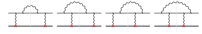
Figure 2: Diagrams contributing to the cross section of Bremsstrahlung.

We define the following family of integrals:

$$j_{n_{1},\ldots,n_{7}}=e^{2\epsilon\gamma_{E}}\int\frac{d^{d}p_{2}d^{d}k_{1}}{\pi^{d}}\frac{\prod_{k=1}^{3}\delta^{(n_{k}-1)}(-D_{k})}{D_{4}^{n_{4}}D_{5}^{n_{5}}D_{6}^{n_{6}}D_{7}^{n_{7}}}$$ (31)

where

$$D_{1}=n\cdot\left(k_{1}-p_{1}+p_{2}\right),\ D_{2}=p_{2}^{2}-1,\ D_{3}=k_{1}^{2},\ D_{4}=\left(k_{1}-p_{1}+p_{2}\right)^{2},$$

$$D_{5}=\left(k_{1}+p_{2}\right)^{2}-1,\ D_{6}=\left(p_{1}-k_{1}\right)^{2}-1,\ D_{7}=k_{1}\cdot n\,,$$ (32)

$p_{1}$, $p_{2}$, and $k_{1}$ are the momenta of initial electron, final electron, and final photon, respectively, and $n=(1,\boldsymbol{0})$ is the time direction. The last index, $n_{7}$, can not be positive. We find the following 5 master integrals

$$\boldsymbol{j}=(j_{1110000},j_{2110000},j_{1110010},j_{1110020},j_{1111000})^{\intercal},$$ (33)

which obey the differential system

$$\partial_{\varepsilon}\boldsymbol{j}=M\boldsymbol{j}$$ (34)

with

$$M=\left(\begin{array}[]{ccccc}0&1&0&0&0\\ \frac{(1-2\epsilon)(4\epsilon-3)}{\varepsilon^{2}-1}&\frac{3(1-2\epsilon)\varepsilon}{\varepsilon^{2}-1}&0&0&0\\ \frac{(1-2\epsilon)(4\epsilon-3)}{4\epsilon\varepsilon\left(\varepsilon^{2}-1\right)}&\frac{3-8\epsilon}{4\epsilon\left(\varepsilon^{2}-1\right)}&\frac{(2\epsilon-1)\varepsilon}{\varepsilon^{2}-1}&\frac{2}{\varepsilon}&0\\ \frac{(1-2\epsilon)(3-4\epsilon)}{8\epsilon\varepsilon\left(\varepsilon^{2}-1\right)^{2}}&\frac{(2\epsilon-1)\left(4\epsilon\varepsilon^{2}-4\epsilon+3\right)}{8\epsilon\left(\varepsilon^{2}-1\right)^{2}}&\frac{2\epsilon(1-2\epsilon)\varepsilon}{\varepsilon^{2}-1}&-\frac{4\epsilon\varepsilon^{2}-\varepsilon^{2}+1}{\varepsilon\left(\varepsilon^{2}-1\right)}&0\\ 0&-\frac{1}{\varepsilon^{2}-1}&0&0&\frac{(2\epsilon-1)\varepsilon}{\varepsilon^{2}-1}\\ \end{array}\right)$$ (35)

From now on we can use Libra.

• Block[{Print},<​​<Libra`];M =

      {{0,1,0,0,0},{(1-2*e)*(4*e-3)/pp,3*(1-2*e)*w/pp,0,0,0},
{(1-2*e)*(4*e-3)/4/e/w/pp,(3-8*e)/4/e/pp,(2*e-1)*w/pp,2/w,0},
{(1-2*e)*(3-4*e)/8/e/w/pp^2,(2*e-1)*(3/pp+4*e)/8/e/pp,2*e*(1-2*e)*w/pp,
(1-4*e*w^2/pp)/w,0}, {0,-1/pp,0,0,(2*e-1)*w/pp}}//.{pp->w^2-1,
e->\[Epsilon],w->\[CurlyEpsilon]};

• NewDSystem[bsde,$\displaystyle\boldsymbol{\varepsilon}$$\displaystyle\boldsymbol{\to}$M];

The matrix $M$ is block-triangular, and we can use the following command to discover the indices of the diagonal blocks:

• EntangledBlocksIndices[bsde]

• {{1, 2}, {3, 4}, {5}}

First, we have to reduce the diagonal blocks. We start from the block {1,2}. The basic strategy is to copy the block under consideration into temporary variable. Then we can transform this block with a sequence of transformations and apply to the whole matrix the overall transformation.

• ii={1, 2};NewDSystem[b, $\displaystyle\boldsymbol{\varepsilon}$$\displaystyle\boldsymbol{\to}$bsde[[ii,ii]]];

Now we run the visual tool

• t = VisTransformation[b, $\displaystyle\boldsymbol{\varepsilon}$, $\displaystyle\boldsymbol{\epsilon}$];

and immediately see the problem:

The eigenvalues of the matrix residues at $\varepsilon=\pm 1$ are half-integer at $\epsilon=0$. Therefore, we have to make variable change. Following the receipt of Ref. [2], we find the appropriate variable change:

$$\varepsilon=\frac{1+z^{2}}{1-z^{2}}\,.$$ (36)

This variable changes from $0$ to $1$ when $\varepsilon$ increases from $1$ to $\infty$.

There are two different ways to introduce a new variable in Libra. The first one is based on a global variable change. This method has obvious limitations in the case when it is not possible to make the global rationalizing variable change. Another method is based on the command AddNotation’missing. This method is more involved, and we refer to tutorials which come with Libra distribution. For our present example it is sufficient to make the global variable change. So we execute the command

• ChangeVar[bsde,$\displaystyle\boldsymbol{\varepsilon}$$\displaystyle\boldsymbol{\to}$(1+z^2)/(1-z^2),z];

Reducing block $\{1,2\}$.

Next, we return to the reduction of the of the {1,2} block. We reinitialize the temporary matrix

• NewDSystem[b, $\displaystyle\boldsymbol{\varepsilon}$$\displaystyle\boldsymbol{\to}$bsde[[ii,ii]]];

and run the visual tool. Note that the second argument of VisTransformatio’missing should now be $z$ rather than $\varepsilon$. To save space, instead of drawing intermediate pictures of the visual tool, we will indicate the option Highlighted->..’missing to guide the reader by highlighting the buttons to be pressed.

• t = VisTransformation[b, z, $\displaystyle\boldsymbol{\epsilon}$, Highlighted $\displaystyle\boldsymbol{\to}$        {{3}$\displaystyle\boldsymbol{\leftrightarrow}${5},{7}$\displaystyle\boldsymbol{\leftrightarrow}${9},{1}$\displaystyle\boldsymbol{\leftrightarrow}${4},{5}$\displaystyle\boldsymbol{\leftrightarrow}${8},{1}$\displaystyle\boldsymbol{\leftrightarrow}${4},{5}$\displaystyle\boldsymbol{\leftrightarrow}${8}}];Transform[b,t];

Finally, we factor out $\epsilon$ dependence and diagonalize the matrix residue at $z=0$ similarly to the first example:

• t = FactorOut[b, z, $\displaystyle\boldsymbol{\epsilon}$], 1/2] /. _C $\displaystyle\boldsymbol{\to}$ 1;Transform[b,t];t = Transpose@JDSpace[SeriesCoefficient[b[z], z, 0, -1]/ $\displaystyle\boldsymbol{\epsilon}$];Transform[b,t];b[z]

• {{0,-$\displaystyle\frac{\text{24\ $\displaystyle\epsilon$}}{\text{(-1+z)\ (1+z)}}$},{$\displaystyle\frac{\text{4\ $\displaystyle\epsilon$}}{\text{3\ (-1+z)\ (1+z)}}$,$\displaystyle\frac{\text{6\ ($\displaystyle\epsilon$+$\displaystyle\text{z}^{\text{2}}$\ $\displaystyle\epsilon$)}}{\text{(-1+z)\ z\ (1+z)}}$}}

Now we consolidate the sequence of transformations made into one transformation and apply it to the big system bsd’missing:

• t = HistoryConsolidate[b];(*shortcut for OverallTransformation[b][Transform]*)Transform[bsde,t,ii];

Note that third argument of Transfor’missing now indicates the indices of the block

References

- [1] R. N. Lee, J. High Energy Phys. 1504 (2015) 108; [arXiv:1411.0911].
- [2] R. N. Lee, A. A. Pomeransky, arXiv:1707.07856.
- [3] A. Blondel, et al., arXiv:1809.01830, doi:10.23731/CYRM-2019-003.