Stochastic gravitational-wave background in quantum gravity

Abstract

Among all cosmological quantum-gravity or quantum-gravity-inspired scenarios, only very few predict a blue-tilted primordial tensor spectrum. We explore five of them and check whether they can generate a stochastic gravitational-wave background detectable by present and future interferometers: non-local quantum gravity, string-gas cosmology, new ekpyrotic scenario, Brandenberger–Ho non-commutative inflation and multi-fractional spacetimes. We show that non-local quantum gravity is unobservable, while all the other models can reach the strain sensitivity of DECIGO but not that of LIGO-Virgo-KAGRA, LISA or Einstein Telescope. Other quantum-gravity models with red-tilted spectra (most loop quantum cosmologies) or with exceptionally tiny quantum corrections (Wheeler–DeWitt quantum cosmology) are found to be non-detectable.

1 Introduction

The rapidly expanding field of gravitational-wave (GW) astronomy has become an excellent testing ground for old and new ideas about gravity, from general relativity itself to modified gravity models and advanced theories of quantum gravity. Although available observations fully confirmed general relativity [1, 2], there is plenty of room for exploring alternative theories. In particular, quantum gravity can alter the production [3, 4, 5, 6, 7, 8, 9] and the propagation [3, 10, 11, 12, 13, 14, 15, 16, 17, 18] of astrophysical GWs or appear in the strain noise of interferometers as an anomalous signal [16, 19, 20, 21, 22, 23, 24]. In this paper, we consider primordial GWs in quantum gravity and their remnant as a stochastic GW background (SGWB). Since there exist several early universe models in quantum gravity [25], a natural question is whether some of them would be able to leave a characteristic imprint in the SGWB within the sensitivity range of present or future interferometers such as LIGO-Virgo-KAGRA (LVK) [26, 27, 28], LISA [29, 30], Einstein Telescope (ET) [31] and DECIGO [32, 33, 34]. This possibility would become substantial for any model predicting a blue-tilted tensor spectrum (tensor spectral index $n_{\rm t}>0$) with a sufficiently high tensor amplitude (high tensor-to-scalar ratio $r$).

As we will see, it turns out that only very few quantum-gravity models have a blue tilt and most of them fail to produce a large signal since $r$ is very small in the region of the parameter space where $n_{\rm t}>0$ at high frequencies. Four of these models (string-gas cosmology, new ekpyrotic scenario, Brandenberger–Ho non-commutative inflation, multi-fractional inflation) reach the sensitivity threshold of DECIGO. On the other hand, the model of inflation in non-local quantum gravity reduces to ordinary Starobinsky gravity at large frequencies and the spectrum is not lifted. This result is non-trivial because it relies on the full expression of the tensor spectrum rather than on it slow-roll parametrization, which we show to break down due to large non-local corrections.

The five models we will concentrate on are:

1. Non-local Starobinsky inflation [35, 36, 37, 38, 39]. This is a cosmological model arising directly in non-local quantum gravity [40, 41, 42, 43, 44, 45, 46, 47, 48] (see [49] for a review), where the bare gravitational action is second-order in curvature tensors and is endowed with non-local operators, called form factors, with infinitely many derivatives. Second-order curvature terms make the ensuing perturbative field theory renormalizable (as in local Stelle gravity [50, 51, 52, 54, 53, 55, 56]), while non-local operators preserve unitarity. In the local limit expanding the form factors [57], the theory reduces to Starobinsky gravity [58, 59, 60, 61, 62, 63, 64, 65, 66] and, therefore, it can sustain a viable inflationary era [67]. However, if one retains the full non-local form factors, one obtains a non-local version of Starobinsky gravity with different, characteristic inflationary observables in the tensor sector, while the scalar spectrum is unchanged [36]. As we will see below, however, while the tensor index can be positive depending on the choice of form factor, this observable is not sufficient to determine correctly the high-frequency behaviour of the tensor spectrum because higher-order observables get non-negligible non-local corrections. When the full spectrum is considered, the blue tilt found from the tensor index and its running turns out to be spurious and the spectrum remains below the detection threshold of DECIGO and the other experiments.

2. String-gas cosmology [68, 69, 70, 71, 72, 73, 74, 75, 76, 77, 78, 79, 80]. This model, stemming from string theory, produces primordial spectra via a thermal mechanism alternative to inflation. In a compact space, the excitation modes of a thermal ensemble of strings are momentum modes and winding modes. The energy of winding modes decreases with the size of the available space and their number increases with the energy, so that, for an adiabatic process, winding modes dominate the thermal bath in a small space. The temperature of this bath cannot rise indefinitely and reaches a maximal temperature $T_{\rm H}$ called Hagedorn temperature [85]. Since scales smaller than the string length or energies higher than $T_{\rm H}$ are not physically reachable, this mechanism based on string thermodynamics can solve the big-bang problem and also offer an alternative to inflation solving the horizon problem [69]. The universe starts with an almost constant scale factor and a temperature slightly lower than $T_{\rm H}$. Size [81, 82] and shape [83] moduli and the dilaton [84] are stabilized. Both scalar and tensor spectra are generated thermally. In particular, tensor modes are generated by anisotropic pressure terms in the energy-momentum tensor, but near the Hagedorn temperature the thermal bath is dominated by winding modes and the pressure decreases. Thus, there is a decrease of power at low $k$ and a slight blue tilt. Eventually, winding modes decay, three spatial directions open up and the others stay compact, leading to a radiation-dominated era.

3. New ekpyrotic scenario [86, 87, 88]. At the density of the string scale, new degrees of freedom govern the effective four-dimensional cosmological dynamics. At the time when such density is reached, the dynamics is dominated by an S-brane, a space-like hypersurface with zero energy density and negative pressure that induces a transition between a contracting phase (ekpyrosis) and an expanding one. The inhomogeneous perturbations generated before the bounce become almost scale-invariant after passing through it. The amplitude of the tensor spectrum depends on the ratio of the string scale to the Planck scale and is enhanced at super-horizon scales. If the S-brane has zero shear, then $r\lesssim 10^{-3}$, the scalar spectrum is red-tilted and the tensor spectrum is blue-tilted [87].

4. Brandenberger–Ho non-commutative inflation [89, 90, 91, 92, 93, 94, 95, 96, 97, 98, 99, 100, 101]. In this scenario, time and space coordinates do not commute and, as a consequence, the action of the inflaton scalar field driving the early phase of acceleration is decorated with *-products. This structure alters the scalar and tensor primordial spectra in a way that depends on whether the perturbation modes have a wave-length smaller (ultraviolet limit, UV) or larger (infrared limit, IR) than the fundamental length scale appearing in the commutation algebra. In the particular case of natural inflation [102, 103, 104], the IR limit of this model has a blue-tilted tensor spectrum and is compatible with Planck data [101]. Here the time-momentum uncertainty induces a $k$-dependence in the effective mass term of the GW propagation equation. This dependence is inherited by the tensor spectrum and, for a certain choice of parameters, it leads to an enhancement at small scales.

5. Multi-fractional inflation [105]. It arises in multi-fractional spacetimes [106], theories which realize explicitly dimensional flow, a universal feature of quantum gravity such that the dimension of spacetime changes with the probed scale [107, 108, 109, 110]. Integrals and derivatives acquire an anomalous multi-scaling, the action gets a new discrete symmetry at short scales and standard cosmology is modified accordingly [105, 111, 112]. In particular, the scalar and tensor spectrum are modified in such a way that the slow-roll approximation can be relaxed. Here we will consider a previously ignored corner in the parameter space that produces a blue-tilted tensor spectrum. The mechanism to achieve this is purely geometrical: the dimension of spacetime is smaller at small scales/large frequencies but the density of states is the same at all scales, so that small-scale modes have “less spacetime” available and their number increases, hence an enhancement of the power spectrum at large frequencies.

The advantages and disadvantages of these models are listed in Tab. 1.

Advantages Disadvantages Non-local Starobinsky
inflation • Embedded in a full quantum gravity. • Easily understandable physical setting and cosmology. • Acceleration from curvature. • Non-uniqueness of form factors, especially on curved backgrounds. • Unclear UV properties on curved backgrounds. • Difficult to extract phenomenology. String-gas cosmology • Embeddable in string theory. • Few free parameters. • Does not require inflaton. • Analytic temperature dependence $T(k)$ on wave-number unknown. • Requires bounce or short inflation to solve flatness problem. • Early-universe observables not following a slow-roll hierarchy. New ekpyrotic
scenario • Embeddable in string theory. • Does not require inflaton. • Simple consistency relations. • Dilaton and moduli stabilization not under full control. • Complicated bouncing dynamics. • Early-universe observables not following a slow-roll hierarchy. Non-commutative
inflation • Realizes fuzziness (frequent or universal feature in quantum gravity). • Few free parameters, easily falsifiable. • Not embedded in a full quantum gravity. • Large non-commutative effects speculative. • Requires inflaton with selected potential. Multi-fractional
inflation • Realizes dimensional flow (universal feature in quantum gravity). • Very characteristic predictions, easily falsifiable. • Easy analytic treatment. • Does not require special inflaton potentials. • Three out of four theories are not renormalizable quantum gravities. • Bizarre spacetime geometries when $n_{\rm t}>0$. • Requires inflaton.

Table 1: Pros and cons of the main models considered in this paper.

A general positive feature we will discover in this paper is that none of these models requires a fine tuning of the parameters in order to reach the sensitivity threshold of interferometers. However, most of them do not go beyond the level of DECIGO.

In section 2, the definitions and experimental values of the main cosmological observables considered in this paper will be reviewed. In section 3, we summarize models of quantum gravity whose primordial spectra have been investigated in the literature and that, as it turns out, give rise to an undetectable SGWB signal for three possible reasons: (i) the tensor spectrum is red tilted; (ii) the tensor spectrum is blue-tilted but only minimally so; (iii) the tensor spectrum is strongly blue-tilted but the tensor-to-scalar ratio is too small. In section 4, we describe the above models with blue tilt and we compare their SGWB spectrum with the sensitivity curves of LIGO-Virgo-KAGRA, LISA, Einstein Telescope and DECIGO. Bounds from big-bang nucleosynthesis (BBN) are considered in section 5, where we will discuss the impact of including the tensor running and constraints on the models. Section 6 is devoted to a discussion of these results.

2 Cosmological observables

2.1 CMB observables

We collect some definitions and cosmological formulæ of common use. On a Friedmann–Lemaître–Robertson–Walker (FLRW) background with scale factor $a(t)$, the number of e-foldings from the time $t$ of horizon crossing until the end of inflation at $t_{\rm e}$ is

$$\mathcal{N}:=\ln\frac{a(t_{\rm e})}{a(t)}=\int_{t}^{t_{\rm e}}dt^{\prime}\,H(t^{\prime})\,.$$ (2.1)

In particular, $\dot{\mathcal{N}}=-H$, where $H:=\dot{a}/a$ is the Hubble parameter. The first two slow-roll parameters in terms of the Hubble expansion are

$$\epsilon:=-\frac{\dot{H}}{H^{2}}=\frac{d\ln H}{d\mathcal{N}}\,,\qquad\eta:=-\frac{\ddot{H}}{2H\dot{H}}=\epsilon+\frac{1}{2}\frac{d\ln\epsilon}{d\mathcal{N}}\,.$$ (2.2)

The time derivative of $\epsilon$ is second-order in the slow-roll parameters,

$$\dot{\epsilon}=2H\epsilon(\epsilon-\eta)\,.$$ (2.3)

Defining $\epsilon_{V}:=(M_{\rm Pl}^{2}/2)(V_{,\phi}/V)^{2}$ as the first slow-roll parameter in terms of the inflaton potential $V(\phi)$, where $M_{\rm Pl}=(8\pi)^{-1/2}m_{\rm Pl}$ $=(8\pi G)^{-1/2}\approx 2.44\times 10^{18}\,{\rm GeV}$ is the reduced Planck mass, in the slow-roll approximation $\epsilon\simeq\epsilon_{V}$ in standard cosmology, but this relation can change in quantum gravity; an example is given in [113]. Also, in standard cosmology (but not in models with modified Friedmann equations) $\eta=\eta_{\phi}:=-\ddot{\phi}/(H\dot{\phi})$ and the combination (2.3) is usually positive for the most common types of inflationary potential [25]. For instance, for a monomial potential $V\propto\phi^{p}$ (large-field models), one has $\epsilon=p/(4\mathcal{N}+p)$, $\eta=(p-2)/(4\mathcal{N}+p)$ and $\dot{\epsilon}>0$; for small-field models with $V\propto 1-(\phi/\phi_{0})^{p}$ as well as for natural inflation (4.46), one has $\eta<0$, $|\eta|\gg\epsilon$ and $\dot{\epsilon}>0$. In other words, in Einstein gravity the first slow-roll parameter $\epsilon$ typically grows in time until inflation ends at $\epsilon=1$.

Let $\mathcal{P}_{\rm s}(k)$ and $\mathcal{P}_{\rm t}(k)$ be, respectively, the primordial scalar and tensor spectrum as a function of the spatial comoving wave-number $k=|{\bm{k}}|$. An observable of interest is the tensor-to-scalar ratio

$$r:=\frac{\mathcal{P}_{\rm t}}{\mathcal{P}_{\rm s}}\,.$$ (2.4)

These quantities are evaluated at horizon crossing, i.e., whenever the Hubble parameter appears it should be replaced by $H=k/a$. Consequently, derivatives with respect to the wave-number can be translated into time or e-folds derivatives and vice versa:

$$\frac{d}{d\ln k}=\frac{1}{H(1-\epsilon)}\frac{d}{dt}\simeq\frac{1}{H}\frac{d}{dt}=-\frac{d}{d\mathcal{N}}\,.$$ (2.5)

In particular, the tensor spectral index and its running are defined by

$$n_{\rm t}:=\frac{d\ln\mathcal{P}_{\rm t}}{d\ln k}\,,\qquad\alpha_{\rm t}:=\frac{dn_{\rm t}}{d\ln k}\,.$$ (2.6)

In the scalar sector, these observables are replaced by the scalar spectral index $n_{\rm s}-1$ and the scalar running $\alpha_{\rm s}$. In standard cosmology,

$$n_{\rm t}\propto-\epsilon<0\,,\qquad\alpha_{\rm t}\propto-\dot{\epsilon}<0\qquad\textrm{(Einstein gravity)}\,,$$ (2.7)

for what commented below (2.3): the tensor spectrum is red-tilted and it becomes redder at higher $k$. In quantum gravity, the sign of both observables can flip, as we will see in due course.

To compute the SGWB, we will use the direct expression $\mathcal{P}_{\rm t}(k)$ of the primordial tensor spectrum or, wherever possible, the standard parametric form

$$\mathcal{P}_{\rm t}(k)=\mathcal{P}_{\rm t}(k_{0})\,\exp\left[n_{\rm t}(k_{0})\,\ln\frac{k}{k_{0}}+\frac{\alpha_{\rm t}(k_{0})}{2}\left(\ln\frac{k}{k_{0}}\right)^{2}\right],\qquad\mathcal{P}_{\rm t}(k_{0})=r(k_{0})\,\mathcal{P}_{\rm s}(k_{0})\,,$$ (2.8)

where $r$, $n_{\rm t}$ and $\alpha_{\rm t}$ are given by the theory and are calculated at the pivot scale $k_{0}$, while $\mathcal{P}_{\rm s}(k_{0})$ is the measured amplitude of the comoving curvature perturbation. For multi-fractional inflation, we will use a different parametrization.

In some cases, the factor responsible for the enhancement of the SGWB at interferometer scales is the tensor running. During inflation, the running term does not play an important role because $\alpha_{\rm t}\ll 1$ and $[\ln(k/k_{0})]^{2}\ll 1$. However, at higher frequencies $[\ln(k/k_{0})]^{2}$ increases and the running term can be large enough to inflect the spectrum upwards towards the strain sensitivity range of near-future experiments. This effect is consistent with the parametrization (2.8) as long as $\alpha_{\rm t}$ is small, which is the case in the models considered here with the notable exceptions of non-local gravity and string-gas cosmology.

We use the values of cosmological parameters provided by the Planck Legacy release [67] from the Planck+TT+TE+EE+lowE+lensing+BK15+BAO data set at the pivot scale

$$k_{0}=0.05\,{\rm Mpc}^{-1}\,,$$ (2.9)

where one has

$$\mathcal{P}_{\rm s}(k_{0})=2.0989\times 10^{-9}\,,\qquad h=0.6736\,,\qquad\Omega_{\rm m}=0.3153\,.$$ (2.10)

For inflationary observables, the following constraints on $r$, $n_{\rm s}$ and $\alpha_{\rm s}$ were obtained for a $\Lambda$CDM+$r$+$\alpha_{\rm s}$ model:

$$r<0.068\qquad\qquad\qquad\quad\,\, \textrm{(95\% CL)}\,,$$ (2.11a)

$$n_{\rm s}=0.9658\pm 0.0040\qquad\,\,\,\, \textrm{(68\% CL)}\,,$$ (2.11b)

$$\alpha_{\rm s}=-0.0066\pm 0.0070\qquad \textrm{(68\% CL)}\,,$$ (2.11c)

where CL is the confidence level. There are no strong model-independent cosmic microwave background (CMB) constraints on $n_{\rm t}$ and $\alpha_{\rm t}$ but model-dependent consistency relations between $r$ and $n_{\rm t}$ can place an indirect bound on the tensor index.

2.2 GW observables

A gravitational wave is described as a small dimensionless tensor perturbation around a flat homogeneous cosmological background,

$$ds^{2}=a^{2}(\tau)\left\{-d\tau^{2}+\left[\delta_{ij}+h_{ij}(\tau,{\bm{x}})\right]dx^{i}dx^{j}\right\}\,.$$ (2.12)

Here we use the conformal time $\tau$, related to cosmic time $t$ by $d\tau=dt/a(t)$. It is convenient to Fourier transform $h_{ij}(\tau,{\bm{x}})$ as

$$h_{ij}(\tau,{\bm{x}})=\sum_{l=+,\times}\int\frac{d^{3}{\bm{k}}}{(2\pi)^{3/2}}\,\epsilon_{ij}^{l}\,h_{\bm{k}}^{l}(\tau)\,e^{i{\bm{k}}\cdot{\bm{x}}}\,,$$ (2.13)

where the polarization tensor $\epsilon_{ij}^{l}$ satisfies the symmetric, transverse-traceless condition and is normalized by the relation $\sum_{i,j}\epsilon_{ij}^{l}(\epsilon_{ij}^{l^{\prime}})^{\ast}=2\delta^{ll^{\prime}}$.

The energy density $\rho_{\textsc{gw}}$ of GWs in general relativity is the spatial average of the kinetic energy of the perturbation:

$$\rho_{\textsc{gw}}:=\frac{M_{\rm Pl}^{2}}{8a^{2}}\left\langle\left(\partial_{\tau}h_{ij}\right)^{2}+\left(\nabla h_{ij}\right)^{2}\right\rangle=\frac{M_{\rm Pl}^{2}}{4}\int d\ln k\left(\frac{k}{a}\right)^{2}\frac{k^{3}}{\pi^{2}}\sum_{l}\left|h_{\bm{k}}^{l}\right|^{2}\,.$$ (2.14)

The amplitude of the SGWB is commonly characterized by the dimensionless density parameter

$$\Omega_{\textsc{gw}}(k,\tau):=\frac{1}{\rho_{\rm crit}}\frac{d\rho_{\textsc{gw}}}{d\ln k}\,,$$ (2.15)

where $\rho_{\rm crit}:=3M_{\rm Pl}^{2}H_{0}^{2}$ is the critical energy density. The tensor power spectrum is defined as

$$\Delta^{2}_{t}(k,\tau):=\frac{d\langle 0|h_{ij}^{2}|0\rangle}{d\ln k}=\frac{k^{3}}{\pi^{2}}\sum_{l}\left|h^{l}_{{\bm{k}}}\right|^{2}=:\mathcal{P}_{\rm t}(k)\,\mathcal{T}^{2}(k,\tau)\,,$$ (2.16)

where $\mathcal{P}_{\rm t}(k)$ is the primordial tensor power spectrum and $\mathcal{T}(k,\tau)$ is the transfer function describing the deformation of the primordial spectrum by the evolution of GWs after horizon crossing. Therefore, the energy density today can be written as

$$\Omega_{\textsc{gw}}(k,\tau_{0})=\frac{k^{2}}{12a_{0}^{2}H_{0}^{2}}\mathcal{P}_{\rm t}(k)\,\mathcal{T}^{2}(k,\tau_{0})\,,$$ (2.17)

where the subscript 0 indicates quantities evaluated at the present time.

The shape of the transfer function strongly depends on the Hubble expansion history of the universe; for details, see [114]. In the case of the instant reheating scenario, where soon after inflation the universe enters a radiation-dominated phase, the transfer function for the SGWB amplitude today is [115]

$$\mathcal{T}^{2}(k,\tau_{0})=\Omega_{\rm m}^{2}\left[\frac{g_{\ast}(T_{\rm in})}{g_{\ast 0}}\right]\left[\frac{g_{\ast s0}}{g_{\ast s}(T_{\rm in})}\right]^{4/3}\left[\frac{3j_{1}(k\tau_{0})}{k\tau_{0}}\right]^{2}T_{\rm eq}^{2}(k)\,.$$ (2.18)

The first spherical Bessel function $j_{1}(k\tau_{0})$ can be approximated as $j_{1}(k\tau_{0})\simeq 1/(\sqrt{2}k\tau_{0})$ in the limit $k\tau_{0}\rightarrow 0$. The values of the relativistic degrees of freedom $g_{\ast}(T_{\rm in})$ and of its counterpart for entropy $g_{\ast s}(T_{\rm in})$ change depending on the cosmic temperature at which the mode $k$ enters the horizon, and it changes the spectral shape [116]. To incorporate this effect in the GW spectrum, we introduce the fitting function [117]

$$g_{\ast}[T_{\rm in}(k)]=g_{\ast 0}\frac{A_{1}+\tanh\left[-2.5\log_{10}\left(\frac{k/2\pi}{2.5\times 10^{-12}~{}{\rm Hz}}\right)\right]}{A_{1}+1}\,\frac{A_{2}+\tanh\left[-2.0\log_{10}\left(\frac{k/2\pi}{6.0\times 10^{-9}~{}{\rm Hz}}\right)\right]}{A_{2}+1}$$

where $A_{1}=(-1-10.75/g_{\ast 0})/(-1+10.75/g_{\ast 0})$ and $A_{2}=(-1-g_{\rm max}/10.75)/(-1+g_{\rm max}/10.75)$. For $g_{\rm max}$, we assume the sum of the Standard-Model particles, $g_{\rm max}=106.75$. The same formula can be used for the counterpart for entropy $g_{\ast s}(T_{\rm in})$ by replacing $g_{\ast 0}=3.36$ with $g_{\ast s0}=3.91$. The other fitting function $T_{\rm eq}^{2}(k)$ is given by [118]

$$T_{\rm eq}^{2}(k)=1+1.57x_{\rm eq}+3.42x_{\rm eq}^{2},\qquad x_{\rm eq}:=\frac{k}{k_{\rm eq}}\,,$$ (2.19)

where

$$k_{\rm eq}=7.1\times 10^{-2}\,\Omega_{\rm m}h^{2}~{}{\rm Mpc}^{-1}$$ (2.20)

is the comoving wave-number at radiation-matter equivalence, corresponding to $f_{\rm eq}\approx 9.9\times 10^{-17}(\Omega_{\rm m}h^{2}/0.143)\,{\rm Hz}$.

3 Discarding models

Obtaining a primordial blue-tilted tensor spectrum in quantum gravity is difficult. Despite the abundance of viable cosmological inflationary models in quantum gravity, a close scrutiny reveals that most of them predict a red tilt and those that have a blue tilt often lead to unobservable effects because $n_{\rm t}$ or $r$, or both, are too close to zero.

For instance, the large class of flux-compactification models in string cosmology is uniformly characterized by $n_{\rm t}<0$ [25, 119]. A case apart is the old ekpyrotic scenario, which predicts a strongly blue-tilted tensor index $n_{\rm t}=2$ [120]. While early versions of the model are ruled out because they have also a blue-tilted scalar spectrum, in a recent single-field version perturbations are generated before the ekpyrotic phase and the scalar spectrum is safely red-tilted [121, 122]. However, in all the realizations of the model the tensor-to-scalar ratio is exceptionally small and the resulting SGWB is well below the detection threshold of any present or future interferometer [123].

Similarly, we call the Hamiltonian approaches to quantum gravity out of the game. In Wheeler–DeWitt canonical quantum cosmology, the semi-classical limit of the Wheeler–DeWitt equation for the wave-function of the Universe admits two solutions, one which is continuous along the imaginary axis and the other exhibiting a jump at the origin [124, 125]. The continuous solution leads to red-tilted spectra in both the scalar and the tensor sector [126, 127, 128]. The discontinuous solution has been investigated less but the results in the scalar sector [125, 129] indicate an enhancement of power at small scales, i.e., a blue tilt. The quantum correction to the power spectrum is so strongly suppressed during inflation that it plays no role at late times either.

The tensor spectrum of Wheeler–DeWitt quantum cosmology reads

$$\mathcal{P}_{\rm t}(k)\simeq\mathcal{P}_{\rm t}^{(0)}(k)\left[1\pm c\,(\ell_{\rm Pl}H)^{2}\left(\frac{k_{0}}{k}\right)^{3}\right],$$ (3.1)

where $\mathcal{P}_{\rm t}^{(0)}(k)\propto H^{2}$ is the standard spectrum at horizon crossing ($k=aH$), $c>0$ is a known numerical constant, $k_{0}$ is the pivot scale of the experiment (for the CMB, typically $k_{0}=0.05\,{\rm Mpc}^{-1}$ or $k_{0}=0.002\,{\rm Mpc}^{-1}$) and

$$\ell_{\rm Pl}\approx 10^{-35}\,{\rm m}=5\times 10^{-58}\,{\rm Mpc}$$ (3.2)

is the Planck length. The case with blue (respectively, red) tilt corresponds to the $-$ ($+$) sign. The same corrections to the inflationary spectra have been obtained in a similar approach [130, 131, 132]. The strong suppression of the $(\ell_{\rm Pl}H)^{2}\ll 1$ term is further increased at late times by the $(k_{0}/k)^{3}$ factor, since at the frequencies of LISA and DECIGO $k_{0}/k\sim 10^{-15}\,\mbox{--}\,10^{-13}$.

Loop quantum cosmology is another Hamiltonian framework, based on the quantization of gravity in Ashtekar–Barbero variables. There are three main approaches to cosmological perturbations within loop quantum cosmology.

• In the dressed-metric approach [133, 134], the tensor spectrum is red tilted [135, 136].

• In the effective-constraints approach [137], one can consider quantum corrections coming from inverse-volume operators, from holonomies or, more realistically, from both. If one considers only inverse-volume corrections, the inflationary spectra are compatible with observations [113, 138] but the tensor spectrum is red tilted, since $n_{\rm t}\simeq-2\epsilon_{V}-\delta_{\rm inv}$, where $\delta_{\rm inv}(k)>0$ is a positive inverse-volume quantum correction [113]. On the other hand, the case with only holonomy corrections predicts a blue-tilted tensor spectrum but it is ruled out observationally [139]. To the best of our knowledge, the case with both types of corrections has not been explored yet.

• In the hybrid-quantization approach [140, 141, 142], the value and sign of the spectral index $n_{\rm t}(k)$ depend on the background effective solution and, even more importantly, on the vacuum on which to perturb such background. The $k$-dependence of the tensor index can be found via a numerical analysis and it turns out that for some choices of vacuum $n_{\rm t}<0$, while for others the spectrum oscillates rapidly and a blue tilt can be generated at certain frequencies [142, 143]. However, what matters for the formation of a SGWB is the average trend of the spectrum and, in all these cases, it decreases in $k$ when $k$ is sufficiently large. Therefore, it is unlikely that this model could generate a detectable SGWB, for any vacuum choice. A detailed numerical study, which we will not pursue here, could give a more precise answer.

There are other quantum-gravity models where the tilt of the tensor spectrum depends on certain assumptions and parameter choices, as we will describe in the next section.

4 Models with blue tilt

In this section, we investigate in detail several quantum-gravity models predicting blue-tilted GW spectra at CMB scales. We predict the GW amplitude at interferometer scales for each model and compare the theoretical prediction of the GW spectrum with the sensitivity curves of LIGO-Virgo-KAGRA (LVK) [26, 27, 28], LISA [29, 30], Einstein Telescope (ET) [31], DECIGO [32, 33, 34] and the future pulsar timing array project by SKA [144].

4.1 Non-local Starobinsky inflation

We briefly recall that one of the most favored inflationary models to date [67] is local Starobinsky inflation, based on the Lagrangian [58, 59, 60, 61, 62, 63, 64, 65, 66]

$$\mathcal{L}=\frac{M_{\rm Pl}^{2}}{2}\left(R+\frac{R^{2}}{6m^{2}}\right),$$ (4.1)

where $m$ is a mass scale. While this cosmological model is not based on a local theory of quantum gravity because, contrary to local Stelle gravity [50, 51, 52, 54, 53, 55, 56], it does not contain Riemann-tensor and Ricci-tensor terms, it can be embedded in non-local quantum gravity. Non-local quantum gravity is a covariant, perturbative quantum field theory of gravity which is unitary and super-renormalizable or finite [40, 41, 42, 43, 44, 45, 46, 47, 48] (see [49] for a review). The fundamental action is second-order in curvature tensors and infinite-order in spacetime derivatives. As is well known from the classic example of local Stelle gravity, having second-order curvature terms makes the theory renormalizable (i.e., ultraviolet divergences are under control, there is only a finite number of divergent Feynman diagrams, and the theory is predictive because it contains a finite number of coupling constants). However, the four derivatives included in the second-order curvature terms are responsible for unstable modes and the quantum theory is not unitary. Probability is conserved, and renormalizability is improved, when suitable nonlocal operators called form factors are inserted in the definition of the classical Lagrangian, which is

$$S=\frac{M_{\rm Pl}^{2}}{2}\int d^{4}x\,\sqrt{|g|}\left[R+R\,\gamma_{\rm S}(\Box)R+C_{\mu\nu\rho\sigma}\gamma_{\rm C}(\Box)C^{\mu\nu\rho\sigma}+V(C)\right],$$ (4.2)

where $C_{\mu\nu\rho\sigma}$ is the Weyl tensor and $V(C)$ is a set of local terms in the Weyl tensor necessary if one wants to make the quantum theory finite instead of just renormalizable. They play no role in the cosmological model because $C$ is identically zero on a FLRW background and the operators in $V$ do not enter the graviton propagator. The form factors $\gamma_{\rm S}$ and $\gamma_{\rm C}$ are chosen in such a way that the theory be renormalizable and free of ghosts on a given background. For instance, on Minkowski spacetime

$$\gamma_{\rm S}(z)=-\frac{1}{6M_{*}^{2}z}\left[e^{{\rm H}_{0}(z)}\left(1-\frac{M_{*}^{2}}{m^{2}}z\right)-1\right],\qquad\gamma_{\rm C}(z)=\frac{1}{2M_{*}^{2}}\frac{e^{{\rm H}_{2}(z)}-1}{z}\,,$$ (4.3)

where ${\rm H}_{0,2}(z)$ are entire functions of the dimensionless combination

$$z:=\frac{\Box}{M_{*}^{2}}\,,$$ (4.4)

and $M_{*}$ is the fundamental mass of the theory. A very general class of functions ${\rm H}_{0,2}$ with benign UV properties are asymptotically polynomial, i.e., they vanish at small $z$ and go as the logarithm of a polynomial of degree $n_{\rm deg}$ at large $z$:

$$\lim_{z\to 0}{\rm H}_{0,2}(z)=0\,,\qquad\lim_{z\to\infty}{\rm H}_{0,2}(z)=\ln|z|^{n_{\rm deg}}\,,$$ (4.5)

where $n_{\rm deg}\geqslant 1$. Therefore, at high energies, $\exp{\rm H}_{0,2}\sim|z|^{n_{\rm deg}}$. The mass $m$ in (4.3) satisfies the hierarchy $m\ll M_{*}\lesssim M_{\rm Pl}$ during inflation. It is associated with a scalar degree of freedom introduced to recover the Starobinsky Lagrangian (4.1) in the local limit (expansion and truncation of the form factors to leading order [57]) but the theory is UV finite and unitary also in the limit $m\to\infty$.

On curved backgrounds, the expressions for $\gamma_{\rm S}$ and $\gamma_{\rm C}$ change. In particular, on a quasi de Sitter background with Ricci scalar $\bar{R}\approx{\rm const}$, the absence of extra ghost degrees of freedom requires [36, 38]

$$\gamma_{\rm S}(z) = -\frac{1}{6M_{*}^{2}(z+2z_{*})}\left[e^{{\rm H}_{0}(z+2z_{*})}\left(1-\frac{M_{*}^{2}}{m^{2}}z\right)-\left(1+\frac{2M_{*}^{2}}{m^{2}}z_{*}\right)\right]\,,$$ (4.6)

$$\gamma_{\rm C}(z) = \left(\frac{z_{*}}{m^{2}}+\frac{1}{2M_{*}^{2}}\right)\frac{e^{{\rm H}_{2}(z-4z_{*})}-1}{z-4z_{*}}\,,$$ (4.7)

where

$$z_{*}:=\frac{R}{6M_{*}^{2}}\,.$$ (4.8)

Equations (4.6) and (4.7) are presented as valid for any curved metric but, strictly speaking, they guarantee ghost freedom only for de Sitter and there is no proof that they would work also for other backgrounds. For this reason, in the following one should regard (4.6) and (4.7) as evaluated on the quasi de Sitter background ($\Box=\bar{\Box}$ in $z$ and $R=\bar{R}$ in $z_{*}$). In the limit $z_{*}\to 0$ (Minkowski spacetime), equations (4.6) and (4.7) reduce to (4.3).

From Planck data, at the CMB pivot scale (2.9) one can write the mass $m$, the Hubble parameter at horizon crossing and the background Ricci scalar at horizon crossing in terms of the reduced Planck mass $M_{\rm Pl}$ and the number of e-foldings corresponding to the CMB pivot scale $\mathcal{N}_{\rm piv}$ [36, 39]:

$$m\simeq\frac{7.15\times 10^{-4}}{\mathcal{N}_{\rm piv}}\,M_{\rm Pl}\,,\qquad\bar{R}\simeq\frac{12.1\times 10^{3}}{\mathcal{N}_{\rm piv}}\,m^{2}\,,$$ (4.9)

so that

$$z_{*}\simeq\frac{1.03\times 10^{-3}}{\mathcal{N}_{\rm piv}^{3}}\frac{M_{\rm Pl}^{2}}{M_{*}^{2}}\,.$$ (4.10)

For Starobinsky inflation, we find $\mathcal{N}_{\rm piv}\approx 54$.

On a de Sitter or quasi de Sitter background, the point $z=z_{*}\neq 0$ corresponds to the pole of the graviton propagator read from the second-order Lagrangianfor the transverse tensor metric perturbation $h_{\mu\nu}=g_{\mu\nu}-\bar{g}_{\mu\nu}$:

$$\delta^{(2)}S=\frac{M_{\rm Pl}^{2}}{2}\int d^{4}x\,\sqrt{|g|}\,h_{ij}\left(\bar{\Box}-\frac{\bar{R}}{6}\right)\,e^{\tilde{\rm H}_{2}(\bar{\Box})}h^{ij}\,,$$ (4.11)

where

$$\tilde{\rm H}_{2}(z):={\rm H}_{2}(z-4z_{*})\,.$$ (4.12)

Note that all the expressions in this section are in the Jordan frame, contrary to the more common Einstein-frame formulation of local Starobinsky gravity and inflationary models [25, 145]. The physical observables must be frame invariant [145]. The only difference with respect to the kinetic term of the graviton in the Jordan frame in standard Starobinsky gravity is the exponential $\exp\tilde{\rm H}_{2}$.

The slow-roll approximation holds, since the background accelerating solution of local or non-local Starobinsky inflation is (quasi) de Sitter [36]:

$$a\simeq a_{\rm c}(t_{\rm e}-t)^{-\frac{1}{6}}\,e^{-\frac{m^{2}}{12}(t_{\rm e}-t)^{2}}\qquad\Longrightarrow\qquad\mathcal{N}\simeq\frac{m^{2}}{12}(t_{\rm e}-t)^{2},$$ (4.13)

where $t_{\rm e}$ is the time at the end of inflation, $a_{\rm c}$ is a constant of energy dimension $-1/6$, and this and the following expressions are valid when $m(t_{\rm e}-t)\gg 1$. Since

$$H\simeq\frac{m^{2}}{6}(t_{\rm e}-t)+\frac{1}{6(t_{\rm e}-t)}\,,$$ (4.14)

$\dot{H}\simeq-m^{2}/6$ and $\ddot{H}\simeq 1/[3(t_{\rm e}-t)^{3}]$, from equations (2.2) and (4.13) one has

$$\epsilon\simeq\frac{1}{2\mathcal{N}}\,,\qquad\eta\simeq\frac{1}{24\mathcal{N}^{2}}\ll\epsilon\,.$$ (4.15)

For later use, we will recast the Hubble parameter at horizon crossing in terms of the comoving wave-number. From (4.13), $t_{\rm e}-t\simeq\sqrt{12\mathcal{N}}/m$, so that (4.14) becomes $H\simeq m\sqrt{\mathcal{N}/3}+m/(12\sqrt{3\mathcal{N}})$. Since the Hubble parameter is approximately constant during inflation, from definition (2.1) one has $\mathcal{N}\simeq\ln(k_{\rm e}/k)$, where $k_{\rm e}$ is the comoving wave-number of the last perturbation crossing the horizon at the end of inflation. Therefore,

$$H(k)\simeq\frac{m}{\sqrt{3}}\left[\left(\ln\frac{k_{\rm e}}{k}\right)^{\frac{1}{2}}+\frac{1}{12}\left(\ln\frac{k_{\rm e}}{k}\right)^{-\frac{1}{2}}\right].$$ (4.16)

The primordial tensor spectrum $\mathcal{P}_{\rm t}$ and the tensor-to-scalar ratio are [36, 37]

$$\mathcal{P}_{\rm t} \simeq \frac{m^{2}}{2\pi^{2}M_{\rm Pl}^{2}}(1-3\epsilon)\,e^{-\tilde{\rm H}_{2}(z_{*})}\,,$$ (4.17)

$$r \simeq \frac{12}{\mathcal{N}^{2}}\,e^{-\tilde{\rm H}_{2}(z_{*})}\,.$$ (4.18)

The expression for $\mathcal{P}_{\rm t}$ is in the next-to-leading order in the slow-roll parameters because, for illustrative purposes, we want to separate the standard part (local Starobinsky inflation, next-to-leading order contribution) and the non-local part (leading order contribution).

To calculate the tensor spectral index $n_{\rm t}$ [37] and its running $\alpha_{\rm t}$, we use the slow-roll formalism and convert the final expression in terms of $\mathcal{N}$ at the end. Using

$$z_{*}\simeq 2\left(\frac{H}{M_{*}}\right)^{2}\,,\qquad\frac{1}{H}\dot{z}_{*}\simeq-2\epsilon z_{*}\simeq-\frac{z_{*}}{\mathcal{N}}\,,$$ (4.19)

we obtain the tensor spectral index

$$n_{\rm t} \simeq -3\frac{\dot{\epsilon}}{H}-\tilde{\rm H}_{2}^{\prime}(z_{*})\frac{\dot{z}_{*}}{H}\simeq-6\epsilon^{2}+2\epsilon z_{*}\tilde{\rm H}_{2}^{\prime}(z_{*})$$ (4.20)

$$\simeq -\frac{3}{2\mathcal{N}^{2}}+\frac{1}{\mathcal{N}}z_{*}\tilde{\rm H}_{2}^{\prime}(z_{*})\,,$$

where a prime denotes the first derivative with respect to $z_{*}$. Similarly, the running of the tensor index is

$$\alpha_{\rm t} \simeq \frac{2}{H}[-6\epsilon\dot{\epsilon}+(\dot{\epsilon}z_{*}+\epsilon\dot{z}_{*})\tilde{\rm H}_{2}^{\prime}(z_{*})+\epsilon z_{*}\dot{z}_{*}\tilde{\rm H}_{2}^{\prime\prime}(z_{*})]$$ (4.21)

$$\simeq -4[6\epsilon^{3}+\epsilon\eta z_{*}\tilde{\rm H}_{2}^{\prime}(z_{*})+\epsilon^{2}z_{*}^{2}\tilde{\rm H}_{2}^{\prime\prime}(z_{*})]$$

$$\simeq -\frac{3}{\mathcal{N}^{3}}-\frac{1}{12\mathcal{N}^{3}}z_{*}\tilde{\rm H}_{2}^{\prime}(z_{*})-\frac{1}{\mathcal{N}^{2}}z_{*}^{2}\tilde{\rm H}_{2}^{\prime\prime}(z_{*})\,.$$

Note that the last term dominates in the slow-roll expansion and is higher-order in $z_{*}\ll 1$. More generally, the $l$-th-order observable in the slow-roll approximation is proportional to the $l$-th derivative of the form factor,

$$\mathcal{O}_{l}:=\frac{d^{l}\ln\mathcal{P}_{\rm t}}{(d\ln k)^{l}}\simeq-\left(-\frac{z_{*}}{\mathcal{N}}\right)^{l}\tilde{\rm H}_{2}^{(l)}(z_{*})+O\left(\frac{1}{\mathcal{N}^{l+1}}\right),$$ (4.22)

where $\mathcal{O}_{0}=\ln\mathcal{P}_{\rm t}$, $\mathcal{O}_{1}=n_{\rm t}$, $\mathcal{O}_{2}=\alpha_{\rm t}$, and so on. The second term, sub-dominant, contains the standard slow-roll terms plus some new terms of the same order in $\mathcal{N}$.

As we will see in the following, depending on the choice of the form factor ${\rm H}_{2}(z_{*})$, we can obtain positive values of $n_{t}$ and $\alpha_{t}$ at the CMB scale, which might indicate a large GW amplitude at interferometer scales. However, this is not the case. We will study the GW spectrum using both the power-series approximation (2.8) and the full expression (4.18) and show that, in fact, the former does not give correct predictions at high frequencies.

4.1.1 Kuz’min and Tomboulis form factors

Let us now discuss the form factors ${\rm H}_{0,2}(\Box)$. They must obey the conditions ${\rm H}_{0,2}(0)=0={\rm H}_{0,2}(m^{2})$. Since ${\rm H}_{0}$ plays no role in (4.11), we will not consider it in detail. The form of $\tilde{\rm H}_{2}$ is determined by (i) the allowed form factors in the full theory on Minkowski spacetime with $m\to\infty$, (ii) their generalization to a finite $m$ on Minkowski spacetime, (iii) their generalization to a finite $m$ and a curved background.

On Minkowski spacetime, the quantum theory is especially well defined in the UV in the case of two weakly non-local operators of the asymptotically polynomial type, one proposed by Kuz’min [41]

$${\rm H}_{\rm Kuz}(z):=\alpha\left\{\ln p(z)+\Gamma[0,p(z)]+\gamma_{\textsc{e}}\right\},$$ (4.23)

and the other by Tomboulis [42, 43],

$${\rm H}_{\rm Tom}(z):=\frac{1}{2}\left\{\ln p^{2}(z)+\Gamma[0,p^{2}(z)]+\gamma_{\textsc{e}}\right\},$$ (4.24)

where $\alpha\geqslant 3$, $\Gamma$ is the upper incomplete gamma function with its first argument vanishing, $\gamma_{\textsc{e}}\approx 0.577$ is the Euler–Mascheroni constant and $p(z)$ is a polynomial such that ${\rm Re}\,p(z)>0$.

The generalization of (4.23) and (4.24) to a Starobinsky term is non-trivial and it involves a choice of polynomial $p(z)$ such that UV divergences in momentum integrals are under control (renormalizability) or disappear altogether (finiteness). For instance, in the case of Tomboulis form factor the beta functions of Newton’s constant and the cosmological constant are identically zero and the theory is super-renormalizable provided $p(\Box)\propto m^{2}\Box^{q-5}(\Box^{3}-m^{6})^{2}/(\Box-m^{2})$ for $q\geqslant 6$ [36]. The proportionality coefficient $m^{2}$ is inserted in order to cancel the coefficient in the full form factor and thus ensuring that the beta function of $m$ is a constant [36].

Things become more complicated on curved backgrounds not only because the translation $p(z)\to p(z-4z_{*})$ should be combined with appropriate $m$ factors, but also because the presence of the Ricci scalar in $z_{*}$ renders the theory non-renormalizable. The first issue is not particularly pressing. Although the $m$-dependence has not been worked out on a curved background, one can ignore it because during inflation $m$ is much smaller than the other scales. The second issue is more serious for the field-theoretician, albeit not necessarily for the cosmologist. In flat space, a derivative expansion of $C\gamma_{\rm C}C$ yields an $O(\Box^{2+n})$ leading term, where $n$ is an integer. This is the same order in the propagator $\sim 1/(k^{2})^{2+n}$ and they compensate each other in Feynman diagrams. However, when $R$ factors are present in $\gamma_{\rm C}$ the derivative order increases by 2 and interactions become $O(4+n)$, thus carrying a divergence worse than the propagator. Until superseded by a more formal proof, this heuristic argument suggests that this cosmological model is not fully embedded in a theory of quantum gravity on curved spacetimes.

With this caveat on board, we can still extract phenomenology from the form factors of the theory. The tensor-to-scalar ratio $r$, the tensor index $n_{\rm t}$, and the tensor running $\alpha_{\rm t}$ stemming from ${\rm H}_{\rm Kuz}(z-4z_{*})$ and ${\rm H}_{\rm Tom}(z-4z_{*})$ with $p(z)=(-z)^{q}$ are shown in Fig. 1.

Figure 1: Tensor-to-scalar ratio $r$ (4.18), tensor spectral index $n_{\rm t}$ (4.20) and tensor running $\alpha_{\rm t}$ (4.21) in non-local Starobinsky inflation with Kuz’min form factor (4.23) (left plots) or Tomboulis form factor (4.24) (right plots) with a polynomial $p(z)=(-z)^{q}$ as a function of the ratio $M_{*}/M_{\rm Pl}$, for $\mathcal{N}_{\rm piv}=54$. Left plots: $\alpha=5$ and $q=1,4,7$ (increasing thickness). Right plots: $q=1,3,5$ (increasing thickness).

Although the tensor-to-scalar ratio tends to be very low when $n_{\rm t}$ and $\alpha_{\rm t}$ are maximal, there is a corner of the parameter space where we can expect large values of $n_{\rm t}$ and $\alpha_{\rm t}$ which could enhance the GW amplitude at interferometer scales. However, as we will see below, we should be careful about using the power-series parametrization (2.8) by $n_{\rm t}$ and $\alpha_{\rm t}$.

Equation (4.22) signals a possibly dangerous problem of convergence of the parametrization (2.8) and its higher-order generalizations. Whenever the form factor is such that $\tilde{\rm H}_{2}^{(n)}(z_{*})$ is large, one cannot use the tensor index and the running as a reliable description of the spectrum. Let us condense Kuz’min and Tomboulis form factors (4.23) and (4.24) into a single expression ${\rm H}_{\rm pol}(z)=\alpha\left\{\ln p^{s}(z)+\Gamma[0,p^{s}(z)]+\gamma_{\textsc{e}}\right\}$, where $\alpha=1/2$ and $s=2$ for Tomboulis while $\alpha\geqslant 3$ and $s=1$ for Kuz’min. Expanding for small $z$ (small $p$), one has ${\rm H}_{\rm pol}(z)=\alpha\sum_{j=1}^{+\infty}(-p^{s})^{j}/(j!j)$, so that for $p(z)=(-z)^{q}$ one has

$$\tilde{\rm H}_{\rm pol}^{(l)}(z_{*})=\alpha\sum_{j=1}^{+\infty}(-1)^{j}3^{qsj}\frac{qsj(qsj-1)\cdots(qsj-l+1)}{j!j}z_{*}^{qsj-l}\,.$$ (4.25)

The leading-order term in $\mathcal{O}_{l}$ is $\propto[\alpha(-1)^{j}3^{l}l!/(j!j)]z_{*}^{l}$, where $j=l/(qs)$. This term will be sizable for an arbitrary order $l$ unless $z_{*}\ll 1$, a regime where the non-local effect is small. Therefore, for this class of form factors it is not possible to use the parametrization (2.8) or any of its generalizations, and one must rely on the exact expression of $\mathcal{P}_{\rm t}(k)$. The latter is given by (4.17) with $z_{*}(k)$ given by (4.19) and (4.16):

$$\mathcal{P}_{\rm t}(k)\simeq\frac{m^{2}}{2\pi^{2}M_{\rm Pl}^{2}}\left[1-\frac{3}{2\ln(k_{\rm e}/k)}\right]\,e^{-\tilde{\rm H}_{2}\left[\frac{2H^{2}(k)}{M_{*}^{2}}\right]}\,.$$ (4.26)

Using Kuz’min form factor with $q=7$ and $\alpha=5$ as an example, we compare the power-series parametrization (2.8) with the full expression of the spectrum (4.26) in Fig. 2. As we can see, the power-series expression by $n_{\rm t}$ and $\alpha_{\rm t}$ predicts a very large amplitude which could reach the sensitivity of several interferometer experiments. However, as expected from the above discussion, we see that the spectrum does not converge by adding the higher-order terms (4.22), contrary to the case of the standard inflationary scenario [146]. Comparing with the full spectrum, we find that the parametrization (2.8) is good near the CMB scale but deviates largely from the true spectrum at high frequencies.

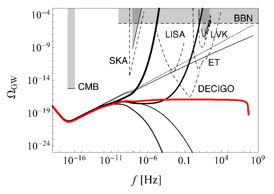
Figure 2: SGWB of non-local Starobinsky inflation with Kuz’min form factor (4.23) with $q=7$ and $\alpha=5$. We compare the GW spectra of the power-series parametrization (2.8) (black solid curves) with the full expression (4.17) (red solid curve). The slow-roll approximation of the 1st to 6th order are calculated using (4.22); the thickness of the line increases with the order. We also show the sensitivity curves of LIGO-Virgo-KAGRA (LVK), SKA, LISA, ET and DECIGO. Shaded regions are excluded by CMB ($r<0.068$), pulsar timing (NANOGrav 11-year data [147]), gravitational-wave (current LIGO data) and BBN observations. Note that we widened the single-frequency CMB constraint to a band in order to make it more visible.

The important message here is that a blue spectrum at the CMB scale does not always mean observable GWs at interferometer scales. In Figs. 3 and 4, we show the SGWB spectrum of, respectively, Kuz’min and Tomboulis form factors for different parameter values, calculated using the full expression (4.26). Figure 1 suggests that we should consider a small ratio $M_{*}/M_{\rm Pl}$ in order to maximize the chance of a blue tilt. On the other hand, recalling the discussion below (4.5), the lower bound of $M_{*}$ is $m$, which is about $10^{-5}M_{\rm Pl}$ if we take (4.9) into account. Taking values of $M_{*}/M_{\rm Pl}$ close to this lower bound, we find that the GW spectra are flattened at high frequencies in all cases, and there are no experiments having enough sensitivity to detect the GWs.

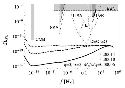
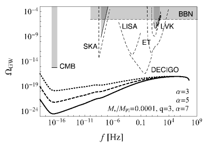
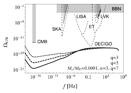
Figure 3: SGWB of non-local Starobinsky inflation with Kuz’min form factor (4.23) for different values of $M_{*}$, $q$ and $\alpha$. Top panel: $q=3$, $\alpha=3$ and $M_{*}/M_{\rm Pl}=0.00014,0.0001,0.00006$ (respectively, dotted, dashed and solid black curve). Bottom left panel: $M_{*}/M_{\rm Pl}=0.0001$, $q=3$ and $\alpha=3,5,7$ (respectively, dotted, dashed and solid black curve). Bottom right panel: $M_{*}/M_{\rm Pl}=0.0001$, $\alpha=3$ and $q=3,5,7$ (respectively, dotted, dashed and solid black curve).

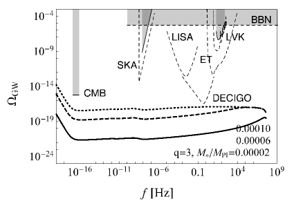
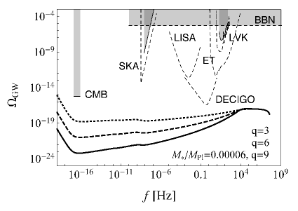
Figure 4: SGWB of non-local Starobinsky inflation with Tomboulis form factor (4.24) for different values of $M_{*}$ and $q$, compared with the sensitivity curves of GW experiments. Left panel: $q=3$, and $M_{*}/M_{\rm Pl}=0.0001,0.00006,0.00002$ (respectively, dotted, dashed and solid black curve). Right panel: $M_{*}/M_{\rm Pl}=0.00006$, and $q=3,6,9$ (respectively, dotted, dashed and solid black curve).

The SGWB at high frequencies matches the ordinary Starobinsky case, i.e., a red-tilted undetectable spectrum. This result is highly non-trivial because a cursory study of the tensor index (4.20), with or without running (4.21), would have led to a radically different conclusion. We can understand the intuitive reason why non-local corrections to the tensor spectrum (4.26) vanish at high frequencies. Equation (4.16) tells us that the Hubble parameter is approximately proportional to a positive power of $\ln(k_{\rm e}/k)>0$ during inflation. Thus, both $H$ and $z_{*}\propto H^{2}$ decrease when $k$ increases. Since $\tilde{\rm H}_{2}$ increases with $z_{*}$, it decreases when $k$ increases and vanishes asymptotically. Therefore, at high frequencies (high $k$) the non-local term $\exp[-\tilde{\rm H}_{2}(z_{*})]$ in the tensor spectrum (4.17) tends to unity,

$$\lim_{k\to\infty}e^{-\tilde{\rm H}_{2}(z_{*})}=1\,,$$ (4.27)

and $\mathcal{P}_{\rm t}$ reduces to the standard Starobinsky spectrum at the frequencies of present and future GW interferometers.

4.1.2 Monomial form factor

Other form factors in non-local quantum gravity predict an unbounded tensor index. These are the monomials

$${\rm H}_{\rm mon}(z):=(-z)^{n}\,.$$ (4.28)

The case $n=1$ corresponds to Wataghin form factor [148], typical in string field theory [149] but very often used also in non-local quantum gravity [150, 151], while for $n=2$ one has Krasnikov form factor [40]. They both generate a strongly suppressed but also strongly blue-tilted tensor spectrum for $M_{*}/M_{\rm Pl}<10^{-4}$, with negative running as shown in Fig. 5.

Figure 5: Tensor-to-scalar ratio (4.18), tensor spectral index (4.20) and tensor running (4.21) with monomial form factor (4.28) as a function of the ratio $M_{*}/M_{\rm Pl}$, for $\mathcal{N}=54$ and with $n=1$ (Wataghin form factor, solid curve) or $n=2$ (Krasnikov form factor, dashed curve).

In Fig. 6, we plot the SGWB spectrum of the model with monomial form factor for different values of $M_{*}/M_{\rm Pl}$, calculated using the full expression (4.17). For the monomial form factors, the $l$-th derivative is given by $\tilde{\rm H}_{\rm mon}^{(l)}(z_{*})=3^{n}n(n-1)\cdots(n-l+1)z_{*}^{n-l}$ and one should take into account all the first $l=n$ slow-roll observables. This means that the tensor index is sufficient to describe the spectrum with Wataghin form factor ($n=1$), while for Krasnikov form factor ($n=2$) one must also consider the tensor running and can safely ignore the running of the running. In fact, we find that the power-series parametrization is in good agreement with the full spectrum when we take into account up to $l=n$ terms. However, the behaviour of the spectrum at high frequencies is similar to the previous cases of Kuz’min and Tomboulis form factors and the SGWB never reaches the detectability threshold of any experiment. This can be understood in terms of the power-series spectrum that, even having a large blue tensor tilt, never has a large GW amplitude because the tensor-to-scalar ratio is highly suppressed at the CMB scale and, furthermore, is suppressed by the tensor running $\alpha_{\rm t}$ at high frequencies.

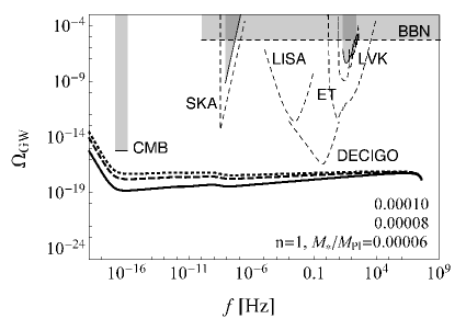
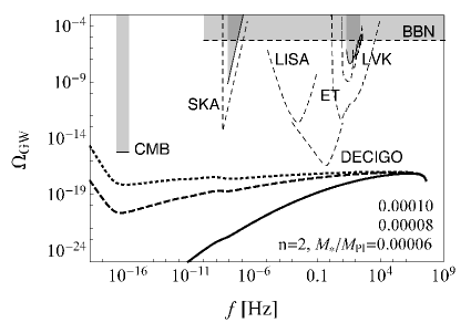
Figure 6: SGWB of non-local Starobinsky inflation with monomial form factor (4.28) for $n=1,2$ (respectively, left and right panel) and $M_{*}/M_{\rm Pl}=0.0001,0.00008,0.00006$ (respectively, dotted, dashed and solid black curve), compared with the sensitivity curves of GW experiments.

4.1.3 Other form factors

One can concoct other phenomenological form factors [38, 39] and here we present two more that respect the asymptotic limits of weakly non-local operators: the difference between two Tomboulis form factors,

$${\rm H}_{\textrm{Tom-Tom}}:={\rm H}_{\rm Tom,1}(z)-{\rm H}_{\rm Tom,2}(z)\,,\qquad{\rm deg}\,p_{1}(z)>{\rm deg}\,p_{2}(z)\,,$$ (4.29)

similar to what proposed in [38], and the difference between Tomboulis and Kuz’min form factors,

$${\rm H}_{\textrm{Tom-Kuz}}:={\rm H}_{\rm Tom}(z)-{\rm H}_{\rm Kuz}(z)\,,\qquad{\rm deg}\,p^{2}_{\rm Tom}(z)>{\rm deg}\,p^{a}_{\rm Kuz}(z)\,.$$ (4.30)

Looking only at leading-order slow-roll observables, they both yield a moderately blue-tilted spectrum (same order as for Tomboulis form factor) with relatively high $r$ (much higher than Tomboulis). However, this blue tilt is an artifact just like for Kuz’min and Tomboulis form factors.

4.2 String-gas cosmology

In this scenario, inflation is replaced by a quasi-static era [79, 80] where thermal fluctuations generate an almost scale-invariant primordial scalar and tensor spectrum, whose derivation is reviewed in [73, 75, 76, 77]. The tensor spectrum is [71, 72, 74]

$$\mathcal{P}_{\rm t}(k)\simeq\frac{1}{4(M_{\rm Pl}l_{\rm st})^{4}}\hat{T}(k)\left[1-\hat{T}(k)\right]\,\ln^{2}\left[\frac{1-\hat{T}(k)}{l_{\rm st}^{2}k^{2}}\right],$$ (4.31)

where $l_{\rm st}$ is the string length scale, $\hat{T}(k):=T(k)/T_{\rm H}$ and the temperature $T(k)$ is evaluated at the time when the mode with comoving wave-number $k$ exits the horizon. As said in the introduction, the form of $T(k)$ is unknown except for its behaviour during the Hagedorn phase ($T\approx{\rm const}\lesssim T_{\rm H}$) and in the following radiation-domination era ($T\sim 1/a$).

Although we have the full expression for the tensor power spectrum in terms of $\hat{T}(k)$, we do not have the correspondence between $\hat{T}(k)$ and $k$. Thus, we do not have a way to plot the GW power spectrum as a function of $k$ using (4.31). Here, relying on the approximation that the SGWB is generated when $T$ is almost constant during the Hagedorn phase, we plot the GW spectrum using the power series expansion (2.8) given in terms of $n_{\rm t}$ and $\alpha_{\rm t}$. However, as we will discuss below, this expression can break down at high frequencies. To show that, we will compare (2.8) with the largest amplitude of GWs obtained from the full expression.

Let us first briefly describe the CMB observables. Since the spectrum is almost scale invariant, the tensor tilt is small but, contrary to the standard inflationary paradigm, positive. In deriving $n_{\rm t}$, usually both the logarithmic term in (4.31) and the running of the spectral index are ignored [74], but the SGBW is sensitive to small variations of the spectral index and its running. Here we will retain the full expressions of $n_{\rm t}$ and the newly derived $\alpha_{\rm t}$ before approximating them.

Since the scalar power spectrum is $\mathcal{P}_{\rm s}\propto\hat{T}/(1-\hat{T})$, the exact expression of the scalar spectral index is

$$n_{\rm s}-1=\frac{d\ln\mathcal{P}_{\rm s}}{d\ln k}=\frac{1}{\hat{T}(1-\hat{T})}\frac{d\hat{T}}{d\ln k}\,,$$ (4.32)

where the factor $1/\hat{T}$ is usually approximated to 1 [74]. Since $\hat{T}\lesssim 1$ and $\hat{T}$ decreases with $k$ ($d\hat{T}/d\ln k<0$), an increase of power is observed for small $k$ ($n_{\rm s}-1<0$). A small red tilt in the scalar sector is produced because scalar modes are generated by the energy density, which increases with $T$. The running of the scalar index is negative, as one can appreciate from the approximate consistency relation $\alpha_{\rm s}\simeq-(1-n_{\rm s})$ [152].

Using (4.32), we find

$$n_{\rm t} = \frac{d\ln\mathcal{P}_{\rm t}}{d\ln k}=(1-n_{\rm s})(2\hat{T}-1)-\frac{2[2-(1-n_{\rm s})\hat{T}]}{\ln[(1-\hat{T})(l_{\rm st}k)^{-2}]}$$ (4.33)

$$\simeq (1-n_{\rm s})-\frac{4}{\ln[(1-\hat{T})(l_{\rm st}k)^{-2}]}>0\,.$$

From the first line of (4.33), we obtain

$$\alpha_{\rm t} = -\alpha_{\rm s}(2\hat{T}-1)-2(1-n_{\rm s})^{2}\hat{T}(1-\hat{T})$$ (4.34)

$$-\frac{2\hat{T}[\alpha_{\rm s}+(1-n_{\rm s})^{2}(1-\hat{T})]}{\ln[(1-\hat{T})(l_{\rm st}k)^{-2}]}-\frac{2[2-(1-n_{\rm s})\hat{T}]^{2}}{\ln^{2}[(1-\hat{T})(l_{\rm st}k)^{-2}]}$$

$$\simeq -\alpha_{\rm s}\,,$$

where in the last line we dropped higher-order terms in the $\hat{T}\sim 1$ expansion. Therefore, the running of the tensor index has opposite sign with respect to the scalar running.

A blue-tilted tensor spectrum is one of the characteristic predictions of string-gas cosmology that could be tested if a primordial gravitational signal was discovered. However, in order to get a detectable signal, the small blue tilt should be accompanied by as high as possible an $r$. The tensor-to-scalar ratio depends on the string scale $l_{\rm st}$:

$$r=\frac{9}{4}\left(1-\hat{T}\right)^{2}\ln^{2}\left[\frac{1-\hat{T}}{(l_{\rm st}k)^{2}}\right]\,,$$ (4.35)

where the additional pre-factor $9/4$ compared to [71, 72, 74] comes from the fact that we define the tensor-to-scalar ratio in terms of the two-point function of the comoving curvature perturbation $\mathcal{P}_{\rm s}\propto\langle\mathcal{R}^{2}\rangle$, while [71, 72, 74] use the that of the scalar perturbation $\langle\Phi^{2}\rangle$, which is related to the curvature perturbation $\zeta\simeq\mathcal{R}$ by $\Phi\simeq-(2/3)\zeta$ for a radiation dominated era.

When $l_{\rm st}\sim 10^{-3}\ell_{\rm Pl}$ and $\hat{T}\approx 0.99$, one obtains an observable $r\lesssim O(0.1)$ [74] while respecting non-Gaussianity bounds [153].

Using the power-series parametrization (2.8) and the CMB predictions (4.33)-(4.35), we plot the spectrum of the SGWB of string-gas cosmology in Fig. 7. As seen in (4.33) and (4.34), $n_{\rm t}$ and $\alpha_{\rm t}$ can be expressed in terms of scalar observables $n_{\rm s}$ and $\alpha_{\rm s}$. We use the central values of the Planck constraints (2.11), $n_{\rm s}=0.9658$ and $\alpha_{\rm s}=-0.0066$. We find that the SGWB can reach the sensitivity of DECIGO if the string scale is $l_{\rm st}=10^{3}M_{\rm Pl}^{-1}$ or smaller. However, these curves fail to capture the full spectrum of the model, also because the Planck central values do not respect the consistency relation $\alpha_{\rm s}\simeq-(1-n_{\rm s})$ [152].

In the figure, we also show the upper bound on the GW amplitude obtained from the full expression, which can be obtained as follows. From (4.31), we find that the function takes the maximum value at $\hat{T}(k)\approx 0.5$ when $l_{\rm st}^{2}k^{2}\ll 1$, which is the case for the GW frequencies of our interest, since $l_{\rm st}\sim(3.7\times 10^{39}\,{\rm Hz})^{-1}$ for $l_{\rm st}=10^{3}M_{\rm Pl}^{-1}$. The maximum value is

$$\mathcal{P}_{\rm t,max}\simeq\frac{0.0625}{(M_{\rm Pl}l_{\rm st})^{4}}\,\ln^{2}\left[\frac{0.5}{l_{\rm st}^{2}k^{2}}\right]\,.$$ (4.36)

For example, for $l_{\rm st}=10^{3}M_{\rm Pl}^{-1}$, we find that the function takes the maximum value at $\hat{T}(k)=0.496$ and $\mathcal{P}_{\rm t,max}=1.89\times 10^{-12}$. The upper bounds are plotted as thick dashed lines in the figure and they clearly show that the power-series expansion extrapolated from the CMB scale overestimates the GW amplitude at high frequencies.

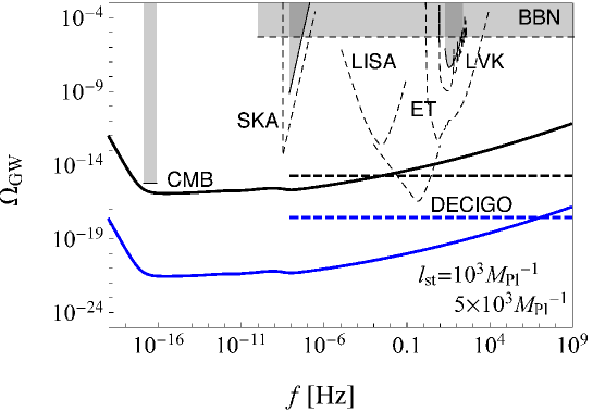
Figure 7: SGWB of string-gas cosmology compared with the sensitivity curves of LIGO-Virgo-KAGRA (LVK), SKA, LISA, ET and DECIGO. The black and blue solid curves corresponds to $l_{\rm st}=10^{3}M_{\rm Pl}^{-1}$ and $5\times 10^{3}M_{\rm Pl}^{-1}$, respectively. We used the central values of the Planck constraints (2.11): $n_{\rm s}=0.9658$ and $\alpha_{\rm s}=-0.0066$. Note that the approximation (2.8) fails for high-frequency GWs, since the corresponding curves go beyond the upper bound on the GW amplitude (dashed lines) obtained from the full expression (4.36).

4.3 New ekpyrotic scenario

In the ekpyrotic universe, two flat 3-branes constitute the boundary of a five-dimensional spacetime and interact with an attractive potential $V(\varphi)$ along a compact fifth dimension parametrized by the radion $\varphi$. These branes can be the orbifold planes of heterotic M-theory (M-theory compactified on $\mathcal{C}_{3}\times S^{1}/\mathbbm{Z}_{2}$, where $\mathcal{C}_{3}$ is a Calabi–Yau space) [154, 155] or the $(3+1)$-dimensional manifolds of a Randall–Sundrum setting [156]. As the branes get closer, the gravitational energy in the bulk is converted into brane kinetic energy. Since the branes are boundary ones, instead of collapsing via tachyon condensation they collide and oscillate back and forth their center of mass along the extra direction. During the collision at coincident branes ($\varphi=-\infty$), part of the brane kinetic energy is converted into matter and radiation. An observer on one of the branes experiences the brane collision as a big bang (vanishing scale factor $a_{\rm E}$ in the Einstein frame) after a period of contraction called ekpyrosis. Even if the fifth dimension experiences a big crunch and it collapses to a point, and even if $a_{\rm E}(t)=0$ for the brane observer, the brane metric in the Jordan frame, the local temperature and the energy density on the brane remain finite at the event.

During the slow contraction phase, a pattern of inhomogeneities is developed. In fact, due to quantum fluctuations the branes are not parallel at all points and they collide at slightly different times in different places. These patches begin their evolution and cooling down from the bounce out of sync, which causes the anisotropies observed in the sky. The spectral properties of this pattern depend on the specific model of ekpyrosis (see [25, chapter 11] for a review). Here we concentrate on the most recent one, of which we already gave a bird’s eye view in the introduction; we refer to [86, 87] for more details. The novelty with respect to old models is the inclusion of an S-brane at high energies, which is expected to be there on theoretical grounds. If the S-brane has vanishing shear, one obtains a viable cosmology with the consistency relation [87]

$$n_{\rm t}=1-n_{\rm s}>0\,,$$ (4.37)

where the scalar spectrum is red-tilted. Therefore,

$$\alpha_{\rm t}=-\alpha_{\rm s}\,.$$ (4.38)

The tensor-to-scalar ratio at the pivot scale is

$$r(k_{0})\simeq\frac{9}{4}\frac{9\cdot 2^{n_{\rm s}}}{\Gamma^{2}\!\left(1-\frac{n_{\rm s}}{2}\right)}(k_{0}\tau_{\rm B})^{2(1-n_{\rm s})}\,(1-n_{\rm s})^{2}\,,$$ (4.39)

where $\Gamma$ is Euler’s function and $\tau_{\rm B}$ is the conformal time at which the string density is reached and the cosmological bounce takes place. Taking the grand-unification scale at $10^{16}$ GeV, we obtain $\tau_{\rm B}=(aH)^{-1}\approx 5.8\times 10^{-24}\,{\rm Mpc}$. With the observed scalar index (2.11b), one has $r(k_{0})\approx(2\,\mbox{--}\,5)\times 10^{-4}$.

Figure 8 shows the SGWB of this model, obtained using the power-series approximation (2.8). The parameters $r$, $n_{\rm t}$ and $\alpha_{\rm t}$ can be expressed in terms of the scalar observables $n_{\rm s}$ and $\alpha_{\rm s}$ and we take $\tau_{\rm B}=5.8\times 10^{-24}\,{\rm Mpc}$. In the figure, we show the case where we use the central values of the Planck constraints (2.11) as well as the cases of minimizing/maximizing the tensor spectrum (largest/smallest values of $n_{\rm s}$ and $\alpha_{\rm s}$ at the $2\sigma$ level). We also show the spectra calculated assuming no tensor running (dotted lines), which differ a lot with respect to the case where we take the running into account. This indicates the importance of the inclusion of the running for predicting the amplitude of high-frequency GWs. We find that, in the most optimistic case with bluest tilt and strongest positive running (at $2\sigma$ in the experimental error), the signal reaches the sensitivity curves of ET and DECIGO.

Note that the evolution during the ekpyrotic phase has not been investigated in detail and, thus, the behaviour of the GW spectrum at high frequency could deviate from the prediction obtained from the power-series parametrization, as was the case for non-local Starobinsky inflation and string gas cosmology. Therefore, the figure only presents a rough estimate on the SGWB amplitude at interferometer scales, inferred from the current constraints of CMB observables.

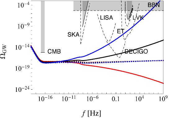
Figure 8: SGWB of the new ekpyrotic scenario compared with the sensitivity curves of LIGO-Virgo-KAGRA (LVK), SKA, LISA, ET and DECIGO. Denoting as $n_{\rm s}^{\rm obs}\pm\delta n_{\rm s}$ and $\alpha_{\rm s}^{\rm obs}\pm\delta\alpha_{\rm s}$ the Planck values (2.11), we plot the worst case minimizing the tensor blue tilt and maximizing the negative tensor running at the $2\sigma$-level ($n_{\rm t}=1-(n_{\rm s}^{\rm obs}+2\delta n_{\rm s})\approx 0.026$, $\alpha_{\rm t}=-(\alpha_{\rm s}^{\rm obs}+2\delta\alpha_{\rm s})\approx-0.007$, red solid curve), the intermediate case taking the central values of the parameters ($n_{\rm t}=1-n_{\rm s}^{\rm obs}\approx 0.034$, $\alpha_{\rm t}=-\alpha_{\rm s}^{\rm obs}\approx 0.007$, black solid curve) and the best case maximizing the tensor blue tilt and the positive tensor running at the $2\sigma$-level ($n_{\rm t}=1-(n_{\rm s}^{\rm obs}-2\delta n_{\rm s})\approx 0.042$, $\alpha_{\rm t}=-(\alpha_{\rm s}^{\rm obs}-2\delta\alpha_{\rm s})\approx 0.021$, blue solid curve). We take $\tau_{\rm B}=5.8\times 10^{-24}\,{\rm Mpc}$, which corresponds to the conformal time at the grand-unification scale $10^{16}$ GeV. The dotted curves correspond to the above cases with no running.

4.4 Brandenberger–Ho non-commutative inflation

In this model, time and space coordinates do not commute, $[\tilde{\tau},x]=i/M^{2}$, where $\tilde{\tau}:=\int dt\,a$ and $x$ is a comoving spatial coordinate. The fundamental mass scale $M$ defines the correction parameter

$$\delta:=\left(\frac{M}{H}\right)^{2}$$ (4.40)

and roughly divides the space of comoving wave-numbers into two regions: a nearly commutative one where the Hubble radius at inflation was larger than the fundamental length ($H\ll M$, $\delta\gg 1$) and perturbations were generated inside the horizon (thus, $k_{\rm p}=k/a\ll M$, where $k_{\rm p}=1/\lambda$ is the proper frequency), and another describing the IR, large-scale perturbations created outside the sub-Planckian horizon ($H\gg M$, $\delta\ll 1$) [89]. The IR limit is more speculative but it has the largest non-commutative effects and it admits inflationary potentials giving rise to observables compatible with data [101]. In this case, and ignoring the UV limit from now on, the spectrum of tensor perturbations (the scalar spectrum has the same shape) is

$$\mathcal{P}_{\rm t}=\mathcal{P}^{(0)}_{\rm t}\,\Sigma^{2}(\delta)\,,$$ (4.41)

where $\mathcal{P}_{\rm t}^{(0)}=\mathcal{P}_{\rm t}(\Sigma\!\!=\!\!1)$ is the amplitude in the commutative limit (Einstein gravity) and $\Sigma(\delta)$ is a function encoding the non-commutative effects. The factor $\Sigma$ multiplies both the tensor and scalar amplitudes, so that their ratio $r$ is the usual one when expressed in terms of $\epsilon$.

To lowest order in the slow-roll parameters, one has $d\ln\Sigma^{2}/d\ln k\simeq\sigma\epsilon$, where $\sigma$ is a function of $\delta$ such that $\dot{\sigma}=O(\epsilon)$ [98]. In the commutative case, $\sigma=0$. The IR model admits two values, $\sigma=2$ and $\sigma=6$, depending on how non-commutativity enters the second-order action for the cosmological perturbations [98]. For instance, in the $\sigma=6$ case, the FLRW 2-sphere is factored out of the total measure, while in the other case it is not. The tensor spectral index is given by

$$n_{\rm t}\simeq-(2-\sigma)\epsilon\,.$$ (4.42)

The scalar index $n_{\rm s}-1$ gets the same correction of $+\sigma\epsilon$. Since we are interested in blue-tilted tensor spectra, we will focus on $\sigma=6$, although we will recall the general formulæ of the model. The tensor-to-scalar ratio reads

$$r\simeq 16\epsilon\simeq-\frac{16}{2-\sigma}n_{\rm t}\,,$$ (4.43)

while the runnings of the tensor spectral index is

$$\alpha_{\rm t}\simeq-2(2-\sigma)\epsilon(\epsilon-\eta)\,,$$ (4.44)

for constant $\sigma$. In particular, for $\sigma=6$, we find

$$n_{\rm t}\simeq\frac{r}{4}\simeq 4\epsilon,\qquad\alpha_{\rm t}\simeq 8\epsilon(\epsilon-\eta)\,.$$ (4.45)

When $\sigma=6$, the tensor spectrum becomes automatically blue-tilted but the scalar spectrum can stay red-tilted for some choices of inflaton potential [101]. A viable inflationary model embedded in this non-commutative setting with red-tilted scalar spectrum is natural inflation [102, 103], characterized by the potential

$$V(\phi)=V_{0}\left(1+\cos\frac{\phi}{\phi_{*}}\right),$$ (4.46)

where $V_{0}>0$ and $\phi_{*}$ is the energy scale at which the global symmetry associated with this model is broken. The field is related to the number of e-foldings by

$$x:=\cos\left(\frac{\phi}{\phi_{*}}\right)=1-\frac{12A}{1+6A}e^{-\frac{\mathcal{N}}{3A}}\,,$$ (4.47)

where $A=(\phi_{*}/M_{\rm Pl})^{2}/3$. Since

$$\epsilon\simeq\epsilon_{V}=\frac{M_{\rm Pl}^{2}}{2}\left(\frac{V_{,\phi}}{V}\right)^{2}=\frac{1}{6A}\frac{1-x}{1+x}=\frac{1}{(1+6A)\,e^{\frac{\mathcal{N}}{3A}}-6A}\,,$$ (4.48)

one has [101]

$$r\simeq\frac{8}{3A}\frac{1-x}{1+x}\,,\qquad n_{\rm t}\simeq\frac{2}{3A}\frac{1-x}{1+x}\,.$$ (4.49)

The large-$A$ limit is excluded by observations, while small or intermediate values of $A$ lie within the likelihood region of Planck+WP+BAO+high-$\ell$ data. For $\sigma=6$ and choosing the pivot wave-number (2.9), one has [101]

$$5.8<A<11\quad(95\,\%\,{\rm CL})\quad{\rm for}\quad\mathcal{N}=50\,\mbox{--}\,60\,.$$ (4.50)

From these expressions, one can see that the typical predictions of this model are $n_{\rm t}=0.004\,\mbox{--}\,0.015$ and $r=0.02\,\mbox{--}\,0.06$. The tensor running is positive, since $\epsilon$ decreases with the number of e-foldings:

$$\alpha_{\rm t}=-4\frac{d\epsilon}{d\mathcal{N}}\simeq\frac{4}{9A^{2}}\frac{1-x}{(1+x)^{2}}>0\,.$$ (4.51)

The SGWB of this model is depicted in Fig. 9 when taking into account up to the second order ($\alpha_{t}$) in the power-series expansion (2.8). As expected by the fact that non-commutativity changes the sign and value of the coefficients in the slow-roll expressions of the observables but not their order of magnitude, the spectrum is enhanced up to the DECIGO sensitivity curve, but barely so, and it does not reach any other interferometer experiment.

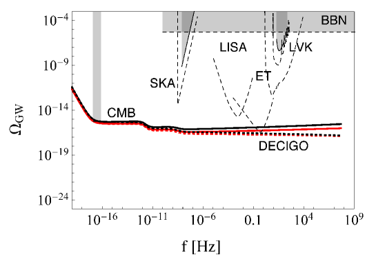
Figure 9: SGWB of the Brandenberger–Ho non-commutative model with $\mathcal{N}=50$ compared with the sensitivity curves of LIGO-Virgo-KAGRA (LVK), SKA, LISA, ET and DECIGO. The red and black solid curves represent the cases with, respectively, $A=7$ and $A=10$, where $A$ is given in (4.47) and the values lie within the allowed interval (4.50). Dotted curves correspond to the commutative cases ($\sigma=0$) with the above values of $A$. Note that we widened the single-frequency CMB constraint to a band in order to make it more visible and that the spectra in the plot satisfy the CMB bound at the pivot scale.

4.5 Multi-fractional inflation

Multi-fractional spacetimes are spacetimes where the clocks and rulers used by the observer register different scaling laws (for instance, linear size versus volume) in copies of the same object with different sizes (for instance, a human-size ball compared with a microscopic one) [106]. This ever-changing geometry is typical of spacetimes arising in quantum gravity [107, 108, 109, 110]. Multi-fractional theories implement it via a modification of the integration measure in the field action and of the kinetic operators acting on the fields, including gravity. While the integral structure is changed according to basic principles of multi-scaling and fractal geometry into a unique parametrization, there are different ways to deform the differential structure. The main ones make use of weighted derivatives, $q$-derivatives or fractional derivatives [106].

Inflation in multi-fractional spacetimes has been studied in the so-called theory with $q$-derivatives [105]. Since we will mainly work in momentum space, we do not have to recall what $q$-derivatives in position space are. Suffice it to say that the gravitational sector of the theory looks like Einstein gravity but with coordinates $x^{\mu}$ replaced by fixed profiles $q^{\mu}(x^{\mu})$ which break ordinary diffeomorphism invariance. These composite coordinates depend on the fundamental lengths of the geometry and also display a discrete scaling symmetry encoded in logarithmic oscillations. Ignoring these oscillations, assuming that geometry has only one fundamental scale and considering an isotropic configuration where all spatial directions scale in the same way, the composite spatial comoving momentum coordinates associated with the $q_{i}(x^{i})$ are

$$p_{i}(k^{i})\simeq k^{i}\left[1+\frac{1}{|\alpha|}\left(\frac{k^{i}}{k_{*}}\right)^{1-\alpha}\right]^{-1},$$ (4.52)

where $k_{*}$ is a fundamental comoving scale and the parameter $\alpha$ can take one of the following ranges of values:

$$\textrm{case 1}: \qquad\!\alpha<0\qquad\textrm{(UV modification of gravity)}\,,$$ (4.53)

$$\textrm{case 2}: 0<\alpha<1\qquad\textrm{(UV modification of gravity)}\,,$$ (4.54)

$$\textrm{case 3}: \qquad\!\alpha>1\qquad\textrm{(IR modification of gravity)}\,.$$ (4.55)

An expression similar to (4.52) holds also for the time direction, with fractional parameter $\alpha_{0}$ not necessarily equal to $\alpha$. The Hausdorff dimension of spacetime is the sum of the $\alpha$ parameters, $d_{\rm H}=\sum_{\mu=0}^{D-1}\alpha_{\mu}=\alpha_{0}+(D-1)\alpha$. Therefore, assuming $\alpha_{0}=O(1)$, in $D=4$ topological dimensions spacetime has a smaller dimensionality $d_{\rm H}<4$ in the UV in cases 1 and 2 and a larger dimensionality $d_{\rm H}>4$ in the IR in case 3. In case 1, we assume that the Hausdorff dimension is well defined, i.e.,

$$d_{\rm H}>0\qquad\Longrightarrow\qquad\alpha_{0}>|3\alpha|\,.$$ (4.56)

Cases 1, 2 and 3 are not mutually exclusive. If one takes a three-term generalized polynomial for $p_{i}$ with three different scales $k_{*123}$, one obtains a geometry where the Hausdorff dimension changes in the UV to two different values $d_{\rm H}<4$, $d_{\rm H}=4$ at intermediate scales (general-relativity regime) and an IR regime where $d_{\rm H}>4$. Removing regimes 1 and 2 from the picture, one is left with pure IR multiple modifications of gravity, while removing either regime 1 or regime 2 one ends up with a model with only one exotic UV regime. From now on, we will consider only geometries with one exotic regime (case 1 or 2 or 3). We will call this exotic regime fractional.

Inflation is driven by a scalar field slowly rolling down its potential. In terms of the $q$ coordinates, the inflationary dynamics is the same as in general relativity, and so are the power spectra in terms of the $p$ momenta. In particular, for an isotropic configuration one can write an approximate expression for $p:=\sqrt{p_{1}^{2}(k^{1})+p_{2}^{2}(k^{2})+p_{3}^{2}(k^{3})}$ in terms of the absolute value $|\bm{k}|=\sqrt{k_{1}^{2}+k_{2}^{2}+k_{3}^{2}}$. This is nothing but equation (4.52) where $k=|\bm{k}|$. Since the standard slow-roll approximation is valid in the frame described by $q$ and $p$ coordinates, instead of the parametrization (2.8) one should use

$$\mathcal{P}_{\rm t}(k)=\mathcal{P}_{\rm t}(k_{0})\,\exp\left\{n_{\rm t}(k_{0})\,\ln\frac{p(k)}{p(k_{0})}+\frac{\alpha_{\rm t}(k_{0})}{2}\left[\ln\frac{p(k)}{p(k_{0})}\right]^{2}\right\},\qquad\mathcal{P}_{\rm t}(k_{0})=r(k_{0})\,\mathcal{P}_{\rm s}(k_{0})\,,$$ (4.57)

where $n_{\rm t}<0$ and $\alpha_{\rm t}<0$ as in standard inflationary models (equation (2.7)) and

$$p(k)\simeq k\left[1+\frac{1}{|\alpha|}\left(\frac{k}{k_{*}}\right)^{1-\alpha}\right]^{-1}.$$ (4.58)

The consistency relation between the tensor-to-scalar ratio and the tensor index is the same as in general relativity,

$$r=-8n_{\rm t}\,.$$ (4.59)

We can always identify two regimes whose $k$-range depends on the sign and value of $\alpha$:

General-relativity regime: $$\qquad p(k)\simeq k\,,\qquad P_{\rm t}(k)\sim k^{n_{\rm t}+\frac{1}{2}\alpha_{\rm t}\ln(k/k_{0})}\,,$$ (4.60)

Fractional regime: $$\qquad p(k)\simeq k^{\alpha}\,,\qquad P_{\rm t}(k)\sim k^{\alpha n_{\rm t}+\frac{1}{2}\alpha_{\rm t}\alpha^{2}\ln(k/k_{0})}\,.$$ (4.61)

We can distinguish three cases (Fig. 10).

1. $\alpha<0$. This is the most interesting case for a SGWB. For $k\ll k_{*}$ (large scales, small frequencies), one hits the general-relativity regime, while the fractional regime is reached for $k\gg k_{*}$ (small scales, large frequencies). In the fractional regime, the effective spectral index $\alpha n_{\rm t}$ is positive definite and the spectrum increases at large $k$. From (4.61), the effective tensor running at large frequencies stays negative, $\alpha^{2}\alpha_{\rm t}<0$, and its absolute value is larger than in standard cosmology if $\alpha<-1$. Intuitively, the enhancement of the power spectrum at small scales compared to Einstein gravity occurs because at these scales $d_{\rm H}<4$ but the primordial density is the same at all scales. Therefore, the number of small-scale modes slightly increases while the number of large-scale modes is the same as standard. Hence the spectrum is blue-tilted but with negative running.

2. $0<\alpha<1$. The general-relativity regime (4.60) corresponds to $k\ll k_{*}$ (large scales, small frequencies), while the fractional regime (4.61) corresponds to $k\gg k_{*}$ (small scales, large frequencies), just like in case 1. The effective spectral index $\alpha n_{\rm t}$ is negative and smaller than usual due to the suppression factor $\alpha$. Because of (4.61), also the running is negative and, in particular, at large frequencies $\alpha^{2}\alpha_{\rm t}<0$. This case is the most studied in the literature [105, 111] and corresponds to a theory where geometry is modified in the UV. The geometric interpretation is that in the UV $d_{\rm H}<4$ and there is an increase in the number of modes given the same density. Overall, the tensor spectrum is less red-tilted than in Einstein gravity.

3. $\alpha>1$. The above limits are switched but the result is similar: the effective spectral index $\alpha n_{\rm t}$ is negative, although this time it is larger than usual due to the enhancement factor $\alpha$. The running is negative and, in particular, at large frequencies $\alpha^{2}|\alpha_{\rm t}|$ is larger than in standard cosmology. Again, the geometric interpretation is intuitive: $d_{\rm H}>4$ at large scales or small frequencies and tensor modes have “more spacetime” than in Einstein gravity. Their density is constant, which means that their number decreases at large scales (suppressed spectrum). Since the spectrum is standard at small scales, overall the tensor spectrum is more red-tilted.

Figure 10: Primordial tensor spectrum (4.57) for $\alpha<0$ ($\alpha=-1/2$ thick curve), $0<\alpha<1$ ($\alpha=1/2$, thin curve) or $\alpha>1$ ($\alpha=3/2$, dotted curve), with $k_{*}=10^{-5}$ Mpc^-1 and $n_{\rm t}=-0.01$. The case of Einstein gravity is the dashed line.

Note that the parameters and $k$-dependence of the scalar spectrum are the same (with $n_{\rm t}$ replaced by $n_{\rm s}-1$), so that if the tensor spectrum is blue-tilted, so is the scalar one. This does not constitute a problem if the transition scale $k_{*}$ is large enough, in which case both spectra are red-tilted at the largest inflationary scales $k\lesssim k_{0}$ and the scalar sector respects observational constraints.

Another remark concerns the fact that, as in the rest of the literature, we defined the model in terms of a comoving constant fundamental scale $k_{*}$ rather than a constant fundamental proper scale $k_{{\rm p}*}=k_{*}/a$, as done in the non-commutative model. However, doing so would lead to a model without observable effects in the SGWB. Consider a power-law expansion $a=t^{1/\epsilon}$, so that conformal time is $\tau=\int dt/a\propto t^{1-1/\epsilon}$ and $t\propto\tau^{\epsilon/(\epsilon-1)}$. At horizon crossing ($\tau=1/k$), one has $a^{-1}\propto k^{-1/(1-\epsilon)}\simeq k^{-1-\epsilon}$ during inflation. Instead of the ratio $(k/k_{*})^{1-\alpha}$ in the spectrum (4.57), we would have a physical scale $k_{{\rm p}*}$ and the ratio $[k/(ak_{{\rm p}*})]^{1-\alpha}=(H/k_{{\rm p}*})^{1-\alpha}$, so that the discrimination between UV and IR regimes would be set by the value of the Hubble horizon during inflation (respectively, $H\ll k_{{\rm p}*}$ and $H\gg k_{{\rm p}*}$). Therefore, inflation would take place only in one of these two regimes and all the scales exiting the horizon would be either in the UV or in the IR. However, the frequencies of all present and future GW interferometers (including DECIGO) are not very high and correspond to scales that exited the horizon during inflation. In particular, a blue tilt at the DECIGO frequency scale would imply a blue tilt also during inflation, including in the scalar sector. Contrary to the non-commutative model, the scalar spectrum is guaranteed to be blue-tilted if the tensor spectrum is such, since $P_{\rm s}(k)\sim k^{\alpha(n_{\rm s}-1)}$ and $n_{\rm s}-1<0$. This model would then be unviable.

In order to respect the condition (4.56) while avoiding unnaturally large values of $\alpha_{0}$, which would be difficult to justify theoretically, we consider only $|\alpha|=O(1)$. Another reason to do so is that the effective tensor running $\alpha^{2}\alpha_{\rm t}$ strongly suppresses the high-frequency spectrum if $\alpha=O(10)$. Therefore, this corner of the parameter space would not be verifiable anyway.

As one can see in Fig. 11, for the typical signs and values of $r$, $n_{\rm t}$ and $\alpha_{\rm t}$ of standard inflationary scalar-field models, the theory can reach the DECIGO sensitivity curve if the running effect is negligible and the tensor-to-scalar ratio $r$ is close to the CMB bound (in the figure, $r=0.06$). The running decreases the spectral amplitude at the typical frequencies of interferometers. We see that the effect of running strongly depends on the value of $\alpha$, since the negative running is amplified by $\alpha^{2}$. Here we take $k_{*}=10^{-3}\,{\rm Mpc}^{-1}$, above which scale $\alpha$ is not constrained by the CMB observables of the scalar sector [105]. Note that the results with zero running are not very sensitive to the choice of scale $k_{*}$ (position of the bending point of the spectrum) because $\alpha n_{\rm t}$ is very small, while the running effect strongly depends on the value of $k_{*}$. In the figure, we show the possible largest effect of the fractional regime by taking the minimally allowed value of $k_{*}=10^{-3}\,{\rm Mpc}^{-1}$, while the large suppression can be avoided if we take a larger value of $k_{*}$.

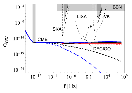
Figure 11: SGWB of multi-fractional inflation with no running ($\alpha_{\rm t}=0$) and $\alpha=-1/2,-3,-5$ (respectively, red, black and blue solid curve), compared with the sensitivity curves of LIGO-Virgo-KAGRA (LVK), SKA, LISA, ET and DECIGO. Here $r=0.06$ and $n_{\rm t}\approx-0.0075$ is given by the consistency relation (4.59) and we take $k_{*}=10^{-3}\,{\rm Mpc}^{-1}$. The dotted curves correspond to the above cases with non-zero running $\alpha_{\rm t}=-0.0001$ (typical order of magnitude of inflationary models). Note that we widened the single-frequency CMB constraint to a band in order to make it more visible and that the spectra in the plot satisfy the CMB bound at the pivot scale.

5 The BBN bound

In the previous section, we have seen cases where a power law is not a good approximation to estimate the amplitude of the SGWB at high frequencies. However, the parametrization with $n_{t}$, $\alpha_{t}$ and so on is still useful to make a first rough prediction from the theory. Here we make a general discussion on the bound from the big-bang nucleosynthesis, which is the ultimate exclusion factor for models where the SGWB grows indefinitely at high frequencies. For example, in Fig. 8, we find a blue-tilted SGBW intersect the BBN exclusion region in the upper right corner. Avoidance of this region places strong bounds on the tensor spectrum and on the underlying model of cosmic seeds, let it be inflation or alternatives such as cosmic-string cosmology or the ekpyrotic universe [157, 158]. In this section, we will show that the upper bound on the tensor index found in [157] becomes stronger in the presence of positive running. We will also apply this result to the models considered above.

5.1 BBN bound with tensor running

The constraint on the number of relativistic degrees of freedom during BBN imposes the upper limit

$$\int_{f_{\rm BBN}}^{f_{\rm e}}\frac{df}{f}\,\Omega_{\textsc{gw}}(f)\,h^{2}<5.6\times 10^{-6}\Delta N_{\nu}\,,$$ (5.1)

where $f=k/(2\pi)$, the frequency $f_{\rm BBN}$ corresponds to the Hubble rate at BBN, $f_{\rm e}$ is a sharp cut-off set by the Hubble rate $H_{\rm e}$ at the end of the period generating cosmic perturbations (inflation or alternatives) and $\Delta N_{\nu}$ parametrizes the effective number of extra relativistic degrees of freedom at the time of BBN. The current upper bound is $\Delta N_{\nu}<0.41$ (BBN+$Y_{p}$+D, 95% CL) [159]. A common procedure is to ignore the logarithmic integral, which is tantamount to considering the dominant contribution from the peak of the spectrum. This gives the constraint on high-frequency ($f>f_{\rm BBN}$) GWs as

$$\Omega_{\textsc{gw}}(f)\,h^{2}<2.3\times 10^{-6}.$$ (5.2)

For a mode entering the horizon during the radiation-dominated phase with $g_{\ast}=g_{\ast s}=106.75$, the transfer function (2.18) becomes

$$\mathcal{T}^{2}(k,\tau_{0})\simeq 0.37\frac{\Omega_{\rm m}^{2}H_{0}^{4}}{k^{2}k_{\rm eq}^{2}}\,.$$ (5.3)

Substituting (2.8) and (5.3) into (2.17), omitting the dependence on the pivot scale $f_{0}$ in the observables $r$, $n_{\rm t}$ and $\alpha_{\rm t}$, and plugging the Planck bound (2.10), we can approximate the spectral shape as

$$\Omega_{\textsc{gw}}(f) = \frac{k^{2}}{12H_{0}^{2}}\mathcal{T}^{2}(f)\,\mathcal{P}_{\rm t}(f)\simeq 0.031\frac{\Omega_{\rm m}^{2}H_{0}^{2}}{k_{\rm eq}^{2}}r\,\mathcal{P}_{\rm s}(f_{0})\left(\frac{f}{f_{0}}\right)^{n_{\rm t}+\frac{\alpha_{\rm t}}{2}\ln\frac{f}{f_{0}}}$$ (5.4)

$$=: \frac{\mathcal{A}}{h^{2}}\,r\left(\frac{f}{f_{0}}\right)^{n_{\rm t}+\frac{\alpha_{\rm t}}{2}\ln\frac{f}{f_{0}}},\qquad\mathcal{A}\approx 1.4\times 10^{-15}\,,$$

which updates the estimate on $\mathcal{A}$ of [160] based on WMAP data and the transfer function of [118]. One can plug (5.4) into (5.1) and integrate exactly, but we checked that the constraints below do not change for any value of $\alpha_{\rm t}>0$ if instead we use (5.2), so that

$$\mathcal{A}\,r\left(\frac{f}{f_{0}}\right)^{n_{\rm t}+\frac{\alpha_{\rm t}}{2}\ln\frac{f}{f_{0}}}<2.3\times 10^{-6}\,.$$ (5.5)

In the limit $\alpha_{\rm t}\to 0$, this reduces to the expression of [157]. Otherwise, we get

$$n_{\rm t}<\frac{\ln\left(\frac{2.3\times 10^{-6}}{\mathcal{A}\,r}\right)}{\ln\frac{f}{f_{0}}}-\frac{\alpha_{\rm t}}{2}\ln\frac{f}{f_{0}}\,.$$ (5.6)

Now we can use the bound (5.6) to place a constraint on the tensor index $n_{\rm t}$. The parameter $\mathcal{A}$ was given in (5.4) and we set $r=0.068$ to its upper bound (2.11a). The pivot scale (2.9) and the BBN scale correspond, respectively, to

$$f_{0}=\frac{k_{0}}{2\pi}\frac{\ell_{\rm Pl}}{t_{\rm Pl}}\approx 7.73\times 10^{-17}\,{\rm Hz}\,,\qquad f_{\rm BBN}=\frac{a_{\rm BBN}H_{\rm BBN}}{2\pi}\frac{m_{\rm Pl}}{t_{\rm Pl}}\approx 10^{-10}\,{\rm Hz}\,,$$ (5.7)

where we multiplied by Planck units conversion factors $\ell_{\rm Pl}/t_{\rm Pl}\approx 9.72\times 10^{-15}\,{\rm Mpc}\,{\rm s}^{-1}$ and $m_{\rm Pl}/t_{\rm Pl}\approx 2.26\times 10^{62}\,{\rm GeV}\,{\rm s}^{-1}$, respectively. For the high-frequency cut-off $f_{\rm e}$, we may choose the comoving Planck scale $a_{\rm e}/t_{\rm Pl}$ for string-gas cosmology and the new ekpyrotic scenario, while for inflationary models it is determined by the Hubble scale at the end of inflation, $H_{\rm e}$. For simplicity, we calculate it for instant reheating, in which case the temperature of the universe at the end of inflation or alternative models is given by

$$T_{\rm e}=\left[\frac{90}{\pi^{2}g_{*}(T_{\rm e})}\right]^{1/4}\left(M_{\rm Pl}H_{\rm e}\right)^{1/2}\,,$$ (5.8)

where we take $g_{*}(T_{\rm e})=106.75$ for the number of relativistic degrees of freedom at the end of inflation. Then the scale factor corresponding to $T_{\rm e}$ is

$$\frac{a_{\rm e}}{a_{0}}=\left[\frac{11}{43}g_{*}(T_{\rm e})\right]^{-1/3}\frac{T_{0}}{T_{\rm e}}\,,$$ (5.9)

where $T_{0}=2.725{\rm K}\approx 2.35\times 10^{-13}\,{\rm GeV}$ is the temperature of the universe today. Setting $T_{\rm e}=10^{16}\,{\rm GeV}$, we get the expansion factor $a_{\rm e}\approx 7.80\times 10^{-30}$ at the grand-unification scale. For string-gas cosmology and the new ekpyrotic scenario, the cut-off scale is the Planck scale dilated up to grand-unification, so that and we find that the high-frequency cut-off is given by

$$f_{\rm e}=f_{\rm Pl}=\frac{a_{\rm e}}{2\pi t_{\rm Pl}}\approx 2.30\times 10^{13}\,{\rm Hz}\,,$$ (5.10)

while

$$f_{\rm e}=f_{\rm inf}=\frac{a_{\rm e}H_{\rm e}}{2\pi}\approx 2.65\times 10^{8}\,{\rm Hz}\,,$$ (5.11)

for grand-unification scale inflation. With these values, in the absence of running we find $n_{\rm t}<0.35$ and $n_{\rm t}<0.42$ respectively for $f_{\rm e}=f_{\rm Pl}$ and $f_{\rm e}=f_{\rm inf}$ with $r=0.068$. Thus, taking the largest energy cut-off gives the tightest constraint on $n_{\rm t}$.

When $\alpha_{\rm t}\neq 0$, the bound (5.6) is strengthened if the running is positive (note that $\ln f_{\rm e}/f_{0}\approx 70$ is positive). To show the effect of running on the BBN bound, we plot this bound as a function of $\alpha_{\rm t}>0$ in Fig. 12. We find that the inclusion of running is important since it dramatically changes the constraint on $n_{t}$. This is because it is much easier to get a large signal at high frequencies when we have positive $\alpha_{t}$, since the effect is enhanced by a factor of $\ln f_{\rm e}/f_{0}\approx 70$ compared to $n_{t}$, as seen in (5.4). When $\alpha_{\rm t}\gtrsim 0.01$, even a red-tilted tensor spectrum can saturate the bound.

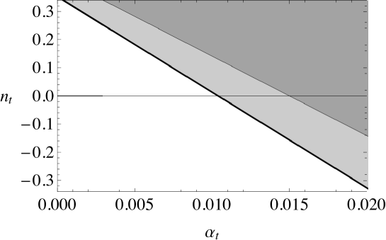
Figure 12: Upper bound (5.6) on the tensor spectral index as a function of the running $\alpha_{\rm t}$, with the frequency and spectral values given in the text, for $f_{\rm e}=f_{\rm Pl}$ (thick line) and $f_{\rm e}=f_{\rm inf}$ (thin line). We fix the tensor-to-scalar ratio to be $r=0.068$ and assume that inflation or its alternative model occurs at the grand-unification scale, i.e. $T_{e}=10^{16}$ GeV. The exclusion region is shaded.

5.2 Application to the models

Let us consider applications of the BBN bound to the five models discussed in section 4.

In the case of models based on scalar-field inflation, i.e, non-local Starobinsky inflation, Brandenberger–Ho non-commutative inflation and multi-fractional inflation, we have a weaker bound from BBN compared to the cases of string-gas cosmology and the new ekpyrotic scenario. This happens because the high-frequency cut-off is at the lower frequency $f_{\rm inf}\ll f_{\rm Pl}$. We have seen that all the former three models do not predict values of $n_{\rm t}$ and $\alpha_{\rm t}$ large enough to reach the BBN bound, so that these scenarios are safe.

In the case of string-gas cosmology and the new ekpyrotic scenario, a SGWB could be produced up to the frequency corresponding to the Planck scale, so that the BBN bound is stronger. For string-gas cosmology, we have shown that there is a theoretical upper bound on the GW amplitude at high frequencies. This upper bound goes beyond the BBN line only when $l_{\rm st}\lesssim 4.5\,M_{\rm Pl}^{-1}$ which is already excluded by the CMB bound. Thus, for this model, the BBN bound does not provide further constraints. For the new ekpyrotic scenario, we have found that the SGWB amplitude can be large at high frequencies if $\alpha_{\rm t}=-\alpha_{\rm s}$ takes a positive value. By taking $f_{\rm e}=f_{\rm Pl}$, we find that $\alpha_{\rm s}>-0.012$ should be satisfied in order not to exceed the BBN bound (this constraint does not depend much on the choice of $n_{\rm t}=1-n_{\rm s}$, since the range of $n_{\rm s}$ is narrow and does not affect the GW amplitude much, as shown in Fig. 8). If we respect this constraint, the SGWB amplitude does not reach the sensitivity curve of ET.

Note that the BBN bound can be avoided if the inflationary phase (or the epoch of perturbations generation by an alternative mechanism) ends with reheating and the evolution of the universe after that follows general relativity. In fact, in that case the tensor spectrum bends down as $\sim k^{n_{\rm t}-2}$ [161], thus evading the BBN constraint [117, 162]. The position of the bending point depends on the reheating temperature $T_{\rm reh}$, ranging from $f\sim 10^{-10}\,{\rm Hz}$ ($T_{\rm reh}=10^{-2}\,{\rm GeV}$, the lowest reheating temperature preserving BBN) to $f\sim 10^{8}\,{\rm Hz}$ ($T_{\rm reh}=10^{15}\,\mbox{--}\,10^{16}\,{\rm GeV}$, instantaneous reheating).

6 Discussion and conclusions

To summarize:

• Non-local Starobinsky inflation. This model is out of reach of any present or future GW experiment because at high frequencies it reduces to standard Starobinsky inflation and, afterwards, to the standard cosmic evolution.

• String-gas cosmology. Depending on the value of the scalar index and running, which determine their tensor counterparts, the SGWB can reach the DECIGO sensitivity range.

• New ekpyrotic scenario. The SGWB reaches the ET and DECIGO sensitivity curve only in the most optimistic choice of parameters. However, if we assume that the spectrum grows continuously towards high frequencies, with no reheating mechanism, then the BBN bound excludes the parameter space accessible by ET.

• Brandenberger–Ho non-commutative inflation. Since this model deviates from standard inflation only in the sign and value of the coefficients in the slow-roll expansions of the observables, the tensor spectrum is blue-tilted but the effect is weak. The SGWB reaches DECIGO sensitivity but it does not go beyond that.

• Multi-fractional inflation. If the tensor-to-scalar ratio is large enough, but still below the observational upper bound (2.11a), then the SGWB can reach DECIGO sensitivity already for natural small values of the fractional parameter $\alpha<0$, for which the negative tensor running is negligible. The signal increases with increasing $|\alpha|$ but, at the same time, so does the suppression effect of the running.

For good or for worse, these results are affected by the running of the tensor index $\alpha_{\rm t}$, which in many cases turns out to be large enough at high frequencies to increase or to lower the tilt up to or below the sensitivity curves of the experiments. Therefore, this often-ignored inflationary observable deserves more attention in quantum gravity, where quantum corrections can compensate the small higher-order slow-roll coefficients in the observables.

However, we also have seen cases where the power-law series expansion, parametrized by $n_{\rm t}$, $\alpha_{\rm t}$ and higher-order slow-roll observables, does not correctly describe the GW spectrum at interferometer scales. For non-local Starobinsky inflation, we compared the spectra calculated using the approximated form and the exact form, and found that even the inclusion of higher-order terms does not help to get the correct prediction of the GW amplitude. This is because, for Kuz’min and Tomboulis form factors, the higher-order derivatives of the quantum-gravity correction term diverges in the regime where the non-local effect is large. For the case of Brandenberger–Ho non-commutative inflation and multi-fractional inflation, we found that corrections are small in general, so that these models preserve a hierarchy of slow-roll parameters and observables and the standard power-law series expansion is a good approximation for all the frequencies of interest. The cases of string-gas cosmology and the new ekpyrotic scenario are more delicate because they are not inflationary models and the evolution of the universe towards the reheating phase has not been investigated in detail. They could even show a non-trivial behaviour at high frequencies which cannot be parametrized by slow-roll observables. Our exploration of quantum-gravity theories with blue-tilted tensor spectrum does not pretend to be exhaustive and there may be other models with such a feature worth studying (e.g., [163]). One such example is pre-big-bang scenario [164], where $r<0.01$ at the pivot scale (2.9) and the SGWB is blue-tilted and can reach the sensitivity of present and future interferometers [165].

Our detailed investigation on the representative five models in section 4 have shown that the commonly used power-law series parametrization of the primordial tensor spectrum is not always appropriate and it must be superseded by a case-by-case analysis using the full spectrum. Furthermore, constraints on the models by the BBN upper bound (and by interferometer experiments in the future) could strongly depend not only on the high-frequency behaviour of the primordial spectrum, but also, as briefly mentioned in section 5, on the reheating mechanism following inflation or its alternatives, which would deserve to be explored more in detail. All these features can enrich the quest for the cosmological imprint of quantum gravity.

References

- [1] B.P. Abbott et al. [LIGO Scientific and Virgo Collaborations], Tests of general relativity with GW150914, Phys. Rev. Lett. 116 (2016) 221101 [Erratum-ibid. 121 (2018) 129902] [arXiv:1602.03841].
- [2] LIGO Scientific Collaboration and Virgo Collaboration, GW190412: observation of a binary-black-hole coalescence with asymmetric masses, Phys. Rev. D 102 (2020) 043015 [arXiv:2004.08342].
- [3] N. Yunes, K. Yagi and F. Pretorius, Theoretical physics implications of the binary black-hole merger GW150914, Phys. Rev. D 94 (2016) 084002 [arXiv:1603.08955].
- [4] A. Kobakhidze, C. Lagger and A. Manning, Constraining noncommutative spacetime from GW150914, Phys. Rev. D 94 (2016) 064033 [arXiv:1607.03776].
- [5] E. Berti, K. Yagi and N. Yunes, Extreme gravity tests with gravitational waves from compact binary coalescences: (I) inspiral-merger, Gen. Rel. Grav. 50 (2018) 46 [arXiv:1801.03208].
- [6] S. Tahura and K. Yagi, Parametrized post-Einsteinian gravitational waveforms in various modified theories of gravity, Phys. Rev. D 98 (2018) 084042 [arXiv:1809.00259].
- [7] A. Maselli, P. Pani, V. Cardoso, T. Abdelsalhin, L. Gualtieri and V. Ferrari, From micro to macro and back: probing near-horizon quantum structures with gravitational waves, Class. Quant. Grav. 36 (2019) 167001 [arXiv:1811.03689].
- [8] S.B. Giddings, S. Koren and G. Treviño, Exploring strong-field deviations from general relativity via gravitational waves, Phys. Rev. D 100 (2019) 044005 [arXiv:1904.04258].
- [9] I. Agullò, V. Cardoso, A. del Rio, M. Maggiore and J. Pullin, Gravitational-wave signatures of quantum gravity. [arXiv:2007.13761].
- [10] J. Ellis, N.E. Mavromatos and D.V. Nanopoulos, Comments on graviton propagation in light of GW150914, Mod. Phys. Lett. A 31 (2016) 1650155 [arXiv:1602.04764].
- [11] G. Calcagni, Lorentz violations in multifractal spacetimes, Eur. Phys. J. C 77 (2017) 291 [arXiv:1603.03046].
- [12] M. Arzano and G. Calcagni, What gravity waves are telling about quantum spacetime, Phys. Rev. D 93 (2016) 124065 [arXiv:1604.00541].
- [13] S. Wang, Exploring the CPT violation and birefringence of gravitational waves with ground- and space-based gravitational-wave interferometers, Eur. Phys. J. C 80 (2020) 342 [arXiv:1712.06072].
- [14] G. Calcagni, S. Kuroyanagi, S. Marsat, M. Sakellariadou, N. Tamanini and G. Tasinato, Gravitational-wave luminosity distance in quantum gravity, Phys. Lett. B 798 (2019) 135000 [arXiv:1904.00384].
- [15] E. Belgacem et al. [LISA Cosmology Working Group], Testing modified gravity at cosmological distances with LISA standard sirens, JCAP 07 (2019) 024 [arXiv:1906.01593].
- [16] G. Calcagni, S. Kuroyanagi, S. Marsat, M. Sakellariadou, N. Tamanini and G. Tasinato, Quantum gravity and gravitational-wave astronomy, JCAP 10 (2019) 012 [arXiv:1907.02489].
- [17] S. Wang and Z.-C. Zhao, Tests of CPT invariance in gravitational waves with LIGO-Virgo catalog GWTC-1, Eur. Phys. J. C 80 (2020) 1032 [arXiv:2002.00396].
- [18] A. Garcia-Chung, J.B. Mertens, S. Rastgoo, Y. Tavakoli and P. Vargas Moniz, Propagation of quantum gravity-modified gravitational waves on a classical FLRW spacetime, arXiv:2012.09366.
- [19] G. Amelino-Camelia, An interferometric gravitational wave detector as a quantum gravity apparatus, Nature 398 (1998) 216 [gr-qc/9808029].
- [20] Y.J. Ng and H. Van Dam, Measuring the foaminess of space-time with gravity-wave interferometers, Found. Phys. 30 (2000) 795 [gr-qc/9906003].
- [21] G. Amelino-Camelia, Quantum-spacetime phenomenology, Living Rev. Rel. 16 (2013) 5 [arXiv:0806.0339].
- [22] P. Bosso, S. Das and R.B. Mann, Potential tests of the generalized uncertainty principle in the advanced LIGO experiment, Phys. Lett. B 785 (2018) 498 [arXiv:1804.03620].
- [23] G. Amelino-Camelia, G. Calcagni and M. Ronco, Imprint of quantum gravity in the dimension and fabric of spacetime, Phys. Lett. B 774 (2017) 630 [arXiv:1705.04876].
- [24] A. Addazi, A. Marcianò and N. Yunes, Can we probe Planckian corrections at the horizon scale with gravitational waves?, Phys. Rev. Lett. 122 (2019) 081301 [arXiv:1810.10417].
- [25] G. Calcagni, Classical and Quantum Cosmology, Springer, Cham, Switzerland (2017).
- [26] B.P. Abbott et al. [LIGO Scientific and Virgo Collaborations], GW150914: implications for the stochastic gravitational wave background from binary black holes, Phys. Rev. Lett. 116 (2016) 131102 [arXiv:1602.03847].
- [27] B.P. Abbott et al. [LIGO Scientific and Virgo Collaborations], GW170817: implications for the stochastic gravitational-wave background from compact binary coalescences, Phys. Rev. Lett. 120 (2018) 091101 [arXiv:1710.05837].
- [28] T. Akutsu et al. [KAGRA Collaboration], KAGRA: 2.5 generation interferometric gravitational wave detector, Nat. Astron. 3 (2019) 35 [arXiv:1811.08079].
- [29] N. Bartolo et al., Science with the space-based interferometer LISA. IV: Probing inflation with gravitational waves, JCAP 12 (2016) 026 [arXiv:1610.06481].
- [30] C. Caprini et al., Reconstructing the spectral shape of a stochastic gravitational wave background with LISA, JCAP 11 (2019) 017 [arXiv:1906.09244].
- [31] M. Maggiore et al., Science case for the Einstein Telescope, JCAP 03 (2020) 050 [arXiv:1912.02622].
- [32] N. Seto, S. Kawamura and T. Nakamura, Possibility of direct measurement of the acceleration of the universe using 0.1-Hz band laser interferometer gravitational wave antenna in space, Phys. Rev. Lett. 87 (2001) 221103 [astro-ph/0108011].
- [33] S. Kawamura et al., The Japanese space gravitational wave antenna: DECIGO, Class. Quant. Grav. 28 (2011) 094011.
- [34] S. Kawamura et al., Current status of space gravitational wave antenna DECIGO and B-DECIGO, arXiv:2006.13545.
- [35] B. Craps, T. De Jonckheere and A.S. Koshelev, Cosmological perturbations in non-local higher-derivative gravity, JCAP 11 (2014) 022 [arXiv:1407.4982].
- [36] A.S. Koshelev, L. Modesto, L. Rachwał and A.A. Starobinsky, Occurrence of exact inflation in non-local UV-complete gravity, JHEP 11 (2016) 067 [arXiv:1604.03127].
- [37] A.S. Koshelev, K.S. Kumar and A.A. Starobinsky, inflation to probe non-perturbative quantum gravity, JHEP 03 (2018) 071 [arXiv:1711.08864].
- [38] K.S. Kumar and L. Modesto, Non-local Starobinsky inflation in the light of future CMB, arXiv:1810.02345.
- [39] A.S. Koshelev, K.S. Kumar, A. Mazumdar and A.A. Starobinsky Non-Gaussianities and tensor-to-scalar ratio in non-local -like inflation, JHEP 06 (2020) 152 [arXiv:2003.00629].
- [40] N.V. Krasnikov, Nonlocal gauge theories, Theor. Math. Phys. 73 (1987) 1184 [Teor. Mat. Fiz. 73 (1987) 235].
- [41] Yu.V. Kuz’min, The convergent nonlocal gravitation, Sov. J. Nucl. Phys. 50 (1989) 1011 [Yad. Fiz. 50 (1989) 1630].
- [42] E.T. Tomboulis, Super-renormalizable gauge and gravitational theories, hep-th/9702146.
- [43] L. Modesto, Super-renormalizable quantum gravity, Phys. Rev. D 86 (2012) 044005 [arXiv:1107.2403].
- [44] T. Biswas, E. Gerwick, T. Koivisto and A. Mazumdar, Towards singularity and ghost free theories of gravity, Phys. Rev. Lett. 108 (2012) 031101 [arXiv:1110.5249].
- [45] T. Biswas, A. Conroy, A.S. Koshelev and A. Mazumdar, Generalized ghost-free quadratic curvature gravity, Class. Quant. Grav. 31 (2014) 015022; Erratum-ibid. 31 (2014) 159501 [arXiv:1308.2319].
- [46] L. Modesto and L. Rachwał, Super-renormalizable and finite gravitational theories, Nucl. Phys. B 889 (2014) 228 [arXiv:1407.8036].
- [47] L. Modesto and L. Rachwał, Universally finite gravitational and gauge theories, Nucl. Phys. B 900 (2015) 147 [arXiv:1503.00261].
- [48] L. Buoninfante, G. Lambiase and A. Mazumdar, Ghost-free infinite derivative quantum field theory, Nucl. Phys. B 944 (2019) 114646 [arXiv:1805.03559].
- [49] L. Modesto and L. Rachwał, Nonlocal quantum gravity: a review, Int. J. Mod. Phys. D 26 (2017) 1730020.
- [50] K.S. Stelle, Renormalization of higher-derivative quantum gravity, Phys. Rev. D 16 (1977) 953.
- [51] K.S. Stelle, Classical gravity with higher derivatives, Gen. Rel. Grav. 9 (1978) 353.
- [52] J. Julve and M. Tonin, Quantum gravity with higher derivative terms, Nuovo Cim. B 46 (1978) 137.
- [53] E.S. Fradkin and A.A. Tseytlin, Renormalizable asymptotically free quantum theory of gravity, Phys. Lett. B 104 (1981) 377.
- [54] E.S. Fradkin and A.A. Tseytlin, Renormalizable asymptotically free quantum theory of gravity, Nucl. Phys. B 201 (1982) 469.
- [55] I.G. Avramidi and A.O. Barvinsky, Asymptotic freedom in higher-derivative quantum gravity, Phys. Lett. B 159 (1985) 269.
- [56] A. Hindawi, B.A. Ovrut and D. Waldram, Consistent spin-two coupling and quadratic gravitation, Phys. Rev. D 53 (1996) 5583 [hep-th/9509142].
- [57] F. Briscese, L. Modesto and S. Tsujikawa, Super-renormalizable or finite completion of the Starobinsky theory, Phys. Rev. D 89 (2014) 024029 [arXiv:1308.1413].
- [58] A.A. Starobinsky, A new type of isotropic cosmological models without singularity, Phys. Lett. B 91 (1980) 99.
- [59] V.F. Mukhanov and G.V. Chibisov, Quantum fluctuation and nonsingular universe, JETP Lett. 33 (1981) 532 [Pis’ma Zh. Eksp. Teor. Fiz. 33 (1981) 549].
- [60] J.D. Barrow and A.C. Ottewill, The stability of general relativistic cosmological theory, J. Phys. A 16 (1983) 2757.
- [61] A.A. Starobinsky, The perturbation spectrum evolving from a nonsingular initially de Sitter cosmology and the microwave background anisotropy, Sov. Astron. Lett. 9 (1983) 302 [Pis’ma Astron. Zh. 9 (1983) 579].
- [62] B. Whitt, Fourth-order gravity as general relativity plus matter, Phys. Lett. B 145 (1984) 176.
- [63] L.A. Kofman, A.D. Linde and A.A. Starobinsky, Inflationary universe generated by the combined action of a scalar field and gravitational vacuum polarization, Phys. Lett. B 157 (1985) 361.
- [64] A.A. Starobinsky and H.-J. Schmidt, On a general vacuum solution of fourth-order gravity, Class. Quant. Grav. 4 (1987) 695.
- [65] K.-i. Maeda, Inflation as a transient attractor in cosmology, Phys. Rev. D 37 (1988) 858.
- [66] K.-i. Maeda, J.A. Stein-Schabes and T. Futamase, Inflation in a renormalizable cosmological model and the cosmic no-hair conjecture, Phys. Rev. D 39 (1989) 2848.
- [67] Y. Akrami et al. [Planck Collaboration], Planck 2018 results. X. Constraints on inflation, Astron. Astrophys. 641 (2020) A10 [arXiv:1807.06211].
- [68] R. Brandenberger and C. Vafa, Superstrings in the early universe, Nucl. Phys. B 316 (1989) 391.
- [69] R. Brandenberger, D.A. Easson and D. Kimberly, Loitering phase in brane gas cosmology, Nucl. Phys. B 623 (2002) 421 [hep-th/0109165].
- [70] A. Nayeri, R.H. Brandenberger and C. Vafa, Producing a scale-invariant spectrum of perturbations in a Hagedorn phase of string cosmology, Phys. Rev. Lett. 97 (2006) 021302 [hep-th/0511140].
- [71] R.H. Brandenberger, A. Nayeri, S.P. Patil and C. Vafa, Tensor modes from a primordial Hagedorn phase of string cosmology, Phys. Rev. Lett. 98 (2007) 231302 [hep-th/0604126].
- [72] R.H. Brandenberger, A. Nayeri, S.P. Patil and C. Vafa, String gas cosmology and structure formation, Int. J. Mod. Phys. A 22 (2007) 3621 [hep-th/0608121].
- [73] R.H. Brandenberger, String gas cosmology, in String Cosmology, J. Erdmenger ed., Wiley, N.Y. (2009) [arXiv:0808.0746].
- [74] R.H. Brandenberger, A. Nayeri and S.P. Patil, Closed string thermodynamics and a blue tensor spectrum, Phys. Rev. D 90 (2014) 067301 [arXiv:1403.4927].
- [75] R.H. Brandenberger, String gas cosmology: progress and problems, Class. Quant. Grav. 28 (2011) 204005 [arXiv:1105.3247].
- [76] R.H. Brandenberger, Unconventional cosmology, Lect. Notes Phys. 863 (2013) 333 [arXiv:1203.6698].
- [77] R.H. Brandenberger, String gas cosmology after Planck, Class. Quant. Grav. 32 (2015) 234002 [arXiv:1505.02381].
- [78] V. Kamali and R. Brandenberger, Creating spatial flatness by combining string gas cosmology and power law inflation, Phys. Rev. D 101 (2020) 103512 [arXiv:2002.09771].
- [79] H. Bernardo, R. Brandenberger and G. Franzmann, String cosmology backgrounds from classical string geometry, [arXiv:2005.08324].
- [80] H. Bernardo, R. Brandenberger and G. Franzmann, Solution of the size and horizon problems from classical string geometry, JHEP 2010 (2020) 155 [arXiv:2007.14096].
- [81] S.P. Patil and R.H. Brandenberger Radion stabilization by stringy effects in general relativity, Phys. Rev. D 71 (2005) 103522 [arXiv:hep-th/0401037].
- [82] S.P. Patil and R.H. Brandenberger The cosmology of massless string modes, JCAP 0601 (2006) 005 [arXiv:hep-th/0502069].
- [83] R.H. Brandenberger, Y.K.E. Cheung and S. Watson, Moduli stabilization with string gases and fluxes, JHEP 0605 (2006) 025 [arXiv:hep-th/0501032].
- [84] R.J. Danos, A.R. Frey and R.H. Brandenberger, Stabilizing moduli with thermal matter and nonperturbative effects, Phys. Rev. D 77 (2008) 126009 [arXiv:0802.1557].
- [85] R. Hagedorn, Statistical thermodynamics of strong interactions at high energies, Nuovo Cim. Suppl. 3 (1965) 147.
- [86] R. Brandenberger and Z. Wang, Nonsingular ekpyrotic cosmology with a nearly scale-invariant spectrum of cosmological perturbations and gravitational waves, Phys. Rev. D 101 (2020) 063522 [arXiv:2001.00638].
- [87] R. Brandenberger and Z. Wang, Ekpyrotic cosmology with a zero-shear S-brane, Phys. Rev. D 102 (2020) 023516 [arXiv:2004.06437].
- [88] R. Brandenberger, K. Dasgupta and Z. Wang, Reheating after S-brane ekpyrosis, Phys. Rev. D 102 (2020) 063514 [arXiv:2007.01203].
- [89] R. Brandenberger and P.-M. Ho, Noncommutative spacetime, stringy spacetime uncertainty principle, and density fluctuations, Phys. Rev. D 66 (2002) 023517 [hep-th/0203119].
- [90] Q.-G. Huang and M. Li, CMB power spectrum from noncommutative spacetime, JHEP 06 (2003) 014 [hep-th/0304203].
- [91] M. Fukuma, Y. Kono and A. Miwa, Effects of space-time noncommutativity on the angular power spectrum of the CMB, Nucl. Phys. B 682 (2004) 377 [hep-th/0307029].
- [92] S. Tsujikawa, R. Maartens and R. Brandenberger, Noncommutative inflation and the CMB, Phys. Lett. B 574 (2003) 141 [astro-ph/0308169].
- [93] Q.-G. Huang and M. Li, Noncommutative inflation and the CMB multipoles, JCAP 11 (2003) 001 [astro-ph/0308458].
- [94] Q.-G. Huang and M. Li, Power spectra in spacetime noncommutative inflation, Nucl. Phys. B 713 (2005) 219 [astro-ph/0311378].
- [95] H. Kim, G.S. Lee and Y.S. Myung, Noncommutative spacetime effect on the slow-roll period of inflation, Mod. Phys. Lett. A 20 (2005) 271 [hep-th/0402018].
- [96] H. Kim, G.S. Lee, H.W. Lee and Y.S. Myung, Second order corrections to noncommutative spacetime inflation, Phys. Rev. D 70 (2004) 043521 [hep-th/0402198].
- [97] R.-G. Cai, A Note on curvature fluctuation of noncommutative inflation, Phys. Lett. B 593 (2004) 1 [hep-th/0403134].
- [98] G. Calcagni, Noncommutative models in patch cosmology, Phys. Rev. D 70 (2004) 103525 [hep-th/0406006].
- [99] G. Calcagni, Consistency relations and degeneracies in (non)commutative patch inflation, Phys. Lett. B 606 (2005) 177 [hep-ph/0406057].
- [100] G. Calcagni and S. Tsujikawa, Observational constraints on patch inflation in noncommutative spacetime, Phys. Rev. D 70 (2004) 103514 [astro-ph/0407543].
- [101] G. Calcagni, S. Kuroyanagi, J. Ohashi and S. Tsujikawa, Strong Planck constraints on braneworld and non-commutative inflation, JCAP 03 (2014) 052 [arXiv:1310.5186].
- [102] K. Freese, J.A. Frieman and A.V. Olinto, Natural inflation with pseudo Nambu–Goldstone bosons, Phys. Rev. Lett. 65 (1990) 3233.
- [103] F.C. Adams, J.R. Bond, K. Freese, J.A. Frieman and A.V. Olinto, Natural inflation: particle physics models, power-law spectra for large-scale structure, and constraints from COBE, Phys. Rev. D 47 (1993) 426 [hep-ph/9207245].
- [104] J.E. Kim, H.P. Nilles and M. Peloso, Completing natural inflation, JCAP 01 (2005) 005 [hep-ph/0409138].
- [105] G. Calcagni, S. Kuroyanagi and S. Tsujikawa, Cosmic microwave background and inflation in multi-fractional spacetimes, JCAP 08 (2016) 039 [arXiv:1606.08449].
- [106] G. Calcagni, Multifractional theories: an unconventional review, JHEP 03 (2017) 138 [arXiv:1612.05632].
- [107] G. ’t Hooft, Dimensional reduction in quantum gravity, in Salamfestschrift, A. Ali, J. Ellis, S. Randjbar-Daemi eds., World Scientific, Singapore (1993) [gr-qc/9310026].
- [108] S. Carlip, Spontaneous dimensional reduction in short-distance quantum gravity?, AIP Conf. Proc. 1196 (2009) 72 [arXiv:0909.3329].
- [109] G. Calcagni, Fractal universe and quantum gravity, Phys. Rev. Lett. 104 (2010) 251301 [arXiv:0912.3142].
- [110] S. Carlip, Dimension and dimensional reduction in quantum gravity, Class. Quant. Grav. 34 (2017) 193001 [arXiv:1705.05417].
- [111] G. Calcagni, Multi-scale gravity and cosmology, JCAP 1312 (2013) 041 [arXiv:1307.6382].
- [112] G. Calcagni, Complex dimensions and their observability, Phys. Rev. D 96 (2017) 046001 [arXiv:1705.01619].
- [113] M. Bojowald, G. Calcagni and S. Tsujikawa, Observational test of inflation in loop quantum cosmology, JCAP 11 (2011) 046 [arXiv:1107.1540].
- [114] S. Kuroyanagi, T. Chiba and N. Sugiyama, Precision calculations of the gravitational wave background spectrum from inflation, Phys. Rev. D 79 (2009) 103501 [arXiv:0804.3249].
- [115] K. Nakayama, S. Saito, Y. Suwa and J. Yokoyama, Probing reheating temperature of the universe with gravitational wave background, JCAP 06 (2008) 020 [arXiv:0804.1827].
- [116] Y. Watanabe and E. Komatsu, Improved calculation of the primordial gravitational wave spectrum in the standard model, Phys. Rev. D 73 (2006) 123515 [astro-ph/0604176].
- [117] S. Kuroyanagi, T. Takahashi and S. Yokoyama, Blue-tilted tensor spectrum and thermal history of the universe, JCAP 02 (2015) 003 [arXiv:1407.4785].
- [118] M.S. Turner, M.J. White and J.E. Lidsey, Tensor perturbations in inflationary models as a probe of cosmology, Phys. Rev. D 48 (1993) 4613 [astro-ph/9306029].
- [119] D. Baumann and L. McAllister, Inflation and String Theory, Cambridge University Press, Cambridge, U.K. (2015) [arXiv:1404.2601].
- [120] J. Khoury, B.A. Ovrut, P.J. Steinhardt and N. Turok, Ekpyrotic universe: colliding branes and the origin of the hot big bang, Phys. Rev. D 64 (2001) 123522 [hep-th/0103239].
- [121] J. Khoury and P.J. Steinhardt, Adiabatic ekpyrosis: scale-invariant curvature perturbations from a single scalar field in a contracting universe, Phys. Rev. Lett. 104 (2010) 091301 [arXiv:0910.2230].
- [122] J. Khoury and P.J. Steinhardt, Generating scale-invariant perturbations from rapidly-evolving equation of state, Phys. Rev. D 83 (2011) 123502 [arXiv:1101.3548].
- [123] L.A. Boyle, P.J. Steinhardt and N. Turok, Cosmic gravitational-wave background in a cyclic universe, Phys. Rev. D 69 (2004) 127302 [hep-th/0307170].
- [124] C. Kiefer and M. Krämer, Quantum gravitational contributions to the CMB anisotropy spectrum, Phys. Rev. Lett. 108 (2012) 021301 [arXiv:1103.4967].
- [125] D. Bini, G. Esposito, C. Kiefer, M. Krämer and F. Pessina, On the modification of the cosmic microwave background anisotropy spectrum from canonical quantum gravity, Phys. Rev. D 87 (2013) 104008 [arXiv:1303.0531].
- [126] D. Brizuela, C. Kiefer and M. Krämer, Quantum-gravitational effects on gauge-invariant scalar and tensor perturbations during inflation: the de Sitter case, Phys. Rev. D 93 (2016) 104035 [arXiv:1511.05545].
- [127] D. Brizuela, C. Kiefer and M. Krämer, Quantum-gravitational effects on gauge-invariant scalar and tensor perturbations during inflation: the slow-roll approximation, Phys. Rev. D 94 (2016) 123527 [arXiv:1611.02932].
- [128] D. Brizuela, C. Kiefer, M. Krämer and S. Robles-Pérez, Quantum-gravity effects for excited states of inflationary perturbations, Phys. Rev. D 99 (2019) 104007 [arXiv:1903.01234].
- [129] G. Calcagni, Observational effects from quantum cosmology, Ann. Phys. (Berlin) 525 (2013) 323 [Erratum-ibid. 525 (2013) A165] [arXiv:1209.0473].
- [130] A.Y. Kamenshchik, A. Tronconi and G. Venturi, Signatures of quantum gravity in a Born–Oppenheimer context, Phys. Lett. B 734 (2014) 72 [arXiv:1403.2961].
- [131] A.Y. Kamenshchik, A. Tronconi and G. Venturi, Quantum gravity and the large scale anomaly, JCAP 04 (2015) 046 [arXiv:1501.06404].
- [132] A.Y. Kamenshchik, A. Tronconi and G. Venturi, Quantum cosmology and the evolution of inflationary spectra, Phys. Rev. D 94 (2016) 123524 [arXiv:1609.02830].
- [133] I. Agulló, A. Ashtekar and W. Nelson, Extension of the quantum theory of cosmological perturbations to the Planck era, Phys. Rev. D 87 (2013) 043507 [arXiv:1211.1354].
- [134] I. Agulló, A. Ashtekar and W. Nelson, The pre-inflationary dynamics of loop quantum cosmology: confronting quantum gravity with observations, Class. Quant. Grav. 30 (2013) 085014 [arXiv:1302.0254].
- [135] I. Agullò and N.A. Morris, Detailed analysis of the predictions of loop quantum cosmology for the primordial power spectra, Phys. Rev. D 92 (2015) 124040 [arXiv:1509.05693].
- [136] B.F. Li, P. Singh and A. Wang, Primordial power spectrum from the dressed metric approach in loop cosmologies, Phys. Rev. D 101 (2020) 086004 [arXiv:1912.08225].
- [137] A. Barrau, M. Bojowald, G. Calcagni, J. Grain and M. Kagan, Anomaly-free cosmological perturbations in effective canonical quantum gravity, JCAP 05 (2015) 051 [arXiv:1404.1018].
- [138] T. Zhu, A. Wang, K. Kirsten, G. Cleaver, Q. Sheng and Q. Wu, Inflationary spectra with inverse-volume corrections in loop quantum cosmology and their observational constraints from Planck 2015 data, JCAP 03 (2016) 046 [arXiv:1510.03855].
- [139] B. Bolliet, A. Barrau, J. Grain and S. Schander, Observational exclusion of a consistent quantum cosmology scenario, Phys. Rev. D 93 (2016) 124011 [arXiv:1510.08766].
- [140] M. Fernández-Méndez, G.A. Mena Marugán and J. Olmedo, Hybrid quantization of an inflationary universe, Phys. Rev. D 86 (2012) 024003 [arXiv:1205.1917].
- [141] L. Castelló Gomar, M. Martín-Benito and G.A. Mena Marugán, Gauge-invariant perturbations in hybrid quantum cosmology, JCAP 06 (2015) 045 [arXiv:1503.03907].
- [142] D. Martín de Blas and J. Olmedo, Primordial power spectra for scalar perturbations in loop quantum cosmology, JCAP 06 (2016) 029 [arXiv:1601.01716].
- [143] L. Castelló Gomar, G.A. Mena Marugán, D. Martín de Blas and J. Olmedo, Hybrid loop quantum cosmology and predictions for the cosmic microwave background, Phys. Rev. D 96 (2017) 103528 [arXiv:1702.06036].
- [144] G. Janssen et al., Gravitational wave astronomy with the SKA, PoS AASKA14 (2015) 037 [arXiv:1501.00127].
- [145] A. De Felice and S. Tsujikawa, theories, Living Rev. Rel. 13 (2010) 3 [arXiv:1002.4928].
- [146] S. Kuroyanagi and T. Takahashi, Higher order corrections to the primordial gravitational wave spectrum and its impact on parameter estimates for inflation, JCAP 10 (2011) 006 [arXiv:1106.3437].
- [147] Z. Arzoumanian et al. [NANOGRAV Collaboration], The NANOGrav 11-year data set: pulsar-timing constraints on the stochastic gravitational-wave background, Astrophys. J. 859 (2018) 47 [arXiv:1801.02617].
- [148] G. Wataghin, Bemerkung über die Selbstenergie der Elektronen, Z. Phys. 88 (1934) 92.
- [149] K. Ohmori, A review on tachyon condensation in open string field theories, hep-th/0102085.
- [150] T. Biswas, A. Mazumdar and W. Siegel, Bouncing universes in string-inspired gravity, JCAP 03 (2006) 009 [hep-th/0508194].
- [151] G. Calcagni and L. Modesto, Nonlocal quantum gravity and M-theory, Phys. Rev. D 91 (2015) 124059 [arXiv:1404.2137].
- [152] R. Brandenberger, G. Franzmann and Q. Liang, Running of the spectrum of cosmological perturbations in string gas cosmology, Phys. Rev. D 96 (2017) 123513 [arXiv:1708.06793].
- [153] B. Chen, Y. Wang, W. Xue and R. Brandenberger, String gas cosmology and non-Gaussianities, arXiv:0712.2477.
- [154] P. Hořava and E. Witten, Heterotic and Type I string dynamics from eleven dimensions, Nucl. Phys. B 460 (1996) 506 [hep-th/9510209].
- [155] P. Hořava and E. Witten, Eleven-dimensional supergravity on a manifold with boundary, Nucl. Phys. B 475 (1996) 94 [hep-th/9603142].
- [156] L. Randall and R. Sundrum, An alternative to compactification, Phys. Rev. Lett. 83 (1999) 4690 [hep-th/9906064].
- [157] A. Stewart and R. Brandenberger, Observational constraints on theories with a blue spectrum of tensor modes, JCAP 08 (2008) 012 [arXiv:0711.4602].
- [158] E.H. Tanin and T. Tenkanen, Gravitational wave constraints on the observable inflation, [arXiv:2004.10702].
- [159] R.H. Cyburt, B.D. Fields, K.A. Olive and T. Yeh, Big Bang Nucleosynthesis: 2015, Rev. Mod. Phys. 88 (2016) 015004 [arXiv:1505.01076].
- [160] S. Chongchitnan and G. Efstathiou, Prospects for direct detection of primordial gravitational waves, Phys. Rev. D 73 (2006) 083511 [astro-ph/0602594].
- [161] N. Seto and J. Yokoyama, Probing the equation of state of the early universe with a space laser interferometer, J. Phys. Soc. Jap. 72 (2003) 3082 [arXiv:gr-qc/0305096].
- [162] S. Kuroyanagi, T. Takahashi and S. Yokoyama, Blue-tilted inflationary tensor spectrum and reheating in the light of NANOGrav results, JCAP 01 (2021) 071 [arXiv:2011.03323].
- [163] A. Dapor and K. Liegener, Modifications to gravitational wave equation from canonical quantum gravity, Eur. Phys. J. C 80 (2020) 741 [arXiv:2002.00834].
- [164] M. Gasperini and G. Veneziano, Pre-big bang in string cosmology, Astropart. Phys. 1 (1993) 317 [arXiv:hep-th/9211021].
- [165] M. Gasperini, Observable gravitational waves in pre-big bang cosmology: an update, JCAP 1612 (2016) 010 [arXiv:1606.07889].