Degeneracy between mass and peculiar acceleration for the double white dwarfs in the LISA band

Abstract

Mass and distance are fundamental quantities to measure in gravitational-wave (GW) astronomy. However, recent studies suggest that the measurement may be biased due to the acceleration of GW source. Here we develop an analytical method to quantify such a bias induced by a tertiary on a double white dwarf (DWD), since DWDs are the most common GW sources in the milli-Hertz band. We show that in a large parameter space the mass is degenerate with the peculiar acceleration, so that from the waveform we can only retrieve a mass of ${\cal M}(1+\Gamma)^{3/5}$, where ${\cal M}$ is the real chirp mass of the DWD and $\Gamma$ is a dimensionless factor proportional to the peculiar acceleration. Based on our analytical method, we conduct mock observation of DWDs by the Laser Interferometer Space Antenna (LISA). We find that in about $9\%$ of the cases the measured chirp mass is biased due to the presence of a tertiary by $(5-30)\%$. Even more extreme cases are found in about a dozen DWDs and they may be misclassified as double neutron stars, binary black holes, DWDs undergoing mass transfer, or even binaries containing lower-mass-gap objects and primordial black holes. The bias in mass also affects the measurement of distance, resulting in a seemingly over-density of DWDs within a heliocentric distance of $1$ kpc as well as beyond $100$ kpc. Our result highlights the necessity of modeling the astrophysical environments of GW sources to retrieve their correct physical parameters.

1 Introduction

Measuring mass is a fundamental problem in Gravitational Wave (GW) astronomy. For sources such as binary black holes (BBHs), binary neutron stars (BNSs) and double white dwarfs (DWDs), the information of mass can be extracted from the inspiral waveform (see Sathyaprakash & Schutz, 2009, for a review). A prerequisite is that the orbital dynamics of the binary is dominated by GW radiation and the GWs propagate freely to the observer. In this ideal situation, the chirp signal, i.e., an increase of GW frequency $f$ with time, is uniquely determined by a quantity called “chirp mass”. It depends on the masses $m_{1}$ and $m_{2}$ of the two compact objects as ${\cal M}=(m_{1}m_{2})^{3/5}/(m_{1}+m_{2})^{1/5}$ (Cutler & Flanagan, 1994). As a result of such a dependence, ${\cal M}$ can be derived from $f$ and its time derivative $\dot{f}$ (“chirp rate” hereafter).

In reality, however, the astrophysical environment of the source could affect the propagation of GWs or perturb the binary orbit. As a result, the chirp signal is distorted and the measurement of the mass could be biased (see Chen, 2020, for a summary). For example, it is well known that the expansion of the universe could stretch the waveform and make the chirp mass appear bigger (Sathyaprakash & Schutz, 2009; Broadhurst et al., 2018; Smith et al., 2018). Such an effect is called the “mass-redshift degeneracy”. It has been generalized recently to include the Doppler and gravitational redshift, to show that the GW sources in the vicinity of supermassive black holes (SMBHs) would also appear more massive (Chen et al., 2019). Moreover, it has been pointed out that the gas around BBHs, by accelerating the orbital shrinkage and increasing $\dot{f}$, could also lead to an overestimation of the chirp masses (Chen & Shen, 2019; Caputo et al., 2020; Chen et al., 2020).

Peculiar acceleration is another environmental factor which could bias the measurement of the mass of a GW source (Bonvin et al., 2017). It is caused by a variation of the centre-of-mass (CoM) velocity of the source. Such a variation could be induced by the gravitational potential of the environment, such as a star cluster, and more likely by a tertiary object since many binaries are in triple systems. The consequence is a time-dependent Doppler shift of the GW frequency (Bonvin et al. 2017, also see Seto 2008 for additional effects when the orbital period of the triple is particularly short). Earlier studies focused on using the frequency shift to identify the GW sources in triple systems, such as an extreme-mass-ratio or intermediate-mass-ratio inspiral with a SMBH tertiary (Yunes et al., 2011; Deme et al., 2020), a BBH orbiting a star or a SMBH (Inayoshi et al., 2017; Meiron et al., 2017; Randall & Xianyu, 2019; Wong et al., 2019; Tamanini et al., 2020), and a DWD accompanied by a star or a planet (Seto, 2008; Robson et al., 2018; Steffen et al., 2018; Tamanini & Danielski, 2019). However, more recent works revealed that the effect due to peculiar acceleration may be indistinguishable from a normal chirp signal when the orbital period of the tertiary is much longer than the observational period. In this case the additional frequency shift induced by the peculiar acceleration could mislead our measurement of $\dot{f}$ and, in turn, cause an bias in the measurement of the chirp mass (Robson et al., 2018; Tamanini et al., 2020).

Such a bias should be more prominent for DWDs than for BBHs or DNSs. First, DWDs have smaller chirp masses, and hence a smaller chirp rate $\dot{f}$ since it depends on ${\cal M}^{5/3}$. Consequently, they are more easily affected by the frequency shift induced by peculiar acceleration (Chen, 2020). Second, DWDs are the most numerous sources in the milli-Hertz (mHz) GW band. They are among the prime targets of the Laser Interferometer Space Antenna (LISA, Nelemans et al., 2001; Seto, 2002; Amaro-Seoane et al., 2017), while BBHs and DNSs are more easily detected by high-frequency detectors, such as LIGO and Virgo (LIGO Scientific Collaboration & Virgo Collaboration, 2019). The relatively low frequency of DWDs further reduces the chirp rate since $\dot{f}\propto f^{11/3}$. Third, both theoretical models (Toonen et al., 2016) and observations (Toonen et al., 2017; Perpinyà-Vallès et al., 2019; Lagos et al., 2020) suggest that a large fraction of DWDs are in triples. Moreover, observations also show that in the Milky Way more than half of the solar-type binaries which have a period shorter than $3$ days are in triple systems (Pribulla & Rucinski, 2006; Tokovinin et al., 2008), and a fraction of $\sim 30$ per cent of the massive stars around the SMBH in the Galactic Centre are in binaries (Pfuhl et al., 2014). After these binary stars evolve into DWDs, it is likely that they are surrounded by tertiaries (Hamers et al., 2013; Stephan et al., 2019).

Indeed, Robson et al. (2018) found cases in which a DWD in a triple system is misidentified by LISA as a isolated DWD with a slight different mass. They also pointed out that the error in the chirp mass would propagate into the estimation of the luminosity distance. However, it is still unclear how common such a bias is among the DWD population in the Milky Way. Given the potential usage of the LISA DWDs in mapping the Milky-Way structure (Cooray & Seto, 2005; Adams et al., 2012; Korol et al., 2019; Breivik et al., 2020), we will study in this paper the impact of peculiar acceleration on the measurement of their chirp masses and distances.

The paper is organized as follows. In Section 2, we derive analytical formulae for the biases in mass and distance induced by the peculiar acceleration. In Section 3, we explore the parameter space of DWDs in which a tertiary induces a significant bias but remains undetectable by LISA. We verify the above analytical results using the numerical matched-filtering technique in Section 4. Then in Section 5, we use a bifurcation model to general a population of DWDs in the LISA band with a realistic fraction of triples. We conduct mock LISA observation of the simulated DWD population in Section 6. Finally, we summarize our results and conclude in Section 7.

2 The effect of peculiar acceleration

The general effect of peculiar acceleration has been discussed in Bonvin et al. (2017). Here we focus on the effect in triple systems containing DWDs. In particular, we derive analytical formulae for the resulting biases in the measurement of the chirp mass and distance. These formulae are useful in our later analysis of a large sample of DWDs.

LISA estimates the chirp mass ${\cal M}$ of a DWD based on two observables, the frequency $f_{e}$ and its time derivative $\dot{f}_{e}$ (“chirp rate” hereafter), where the subscript $e$ denotes the quantities in the rest frame of the source. The details of the method can be found in Cutler & Flanagan (1994) and the result is

$${\cal M}:=\frac{(m_{1}m_{2})^{3/5}}{(m_{1}+m_{2})^{1/5}}={\left(\frac{5c^{5}}{96\pi^{8/3}G^{5/3}}\right)}^{3/5}f_{e}^{-11/5}\dot{f}_{e}^{3/5},$$ (1)

which assumes a circular orbit for the binary. This result suggests that the chirp signal evolves on a timescale of

$$\tau_{\rm gw}:=\frac{f_{e}}{\dot{f}_{e}}\simeq 2.2\times 10^{6}\,\left(\frac{{\cal M}}{0.3\,M_{\odot}}\right)^{-5/3}\left(\frac{f_{e}}{3\,{\rm mHz}}\right)^{-8/3}\,{\rm years}.$$ (2)

Note that this timescale is much longer than the mission duration of LISA, which is about $4-5$ years (Amaro-Seoane et al., 2017).

Using ${\cal M}$ and the GW amplitude $h$, which is the third observable, one can further infer the distance of the DWD as

$$d=\frac{4G}{c^{2}}\frac{{\cal M}}{h}\left(\frac{G}{c^{3}}\pi f_{e}{\cal M}\right)^{2/3}.$$ (3)

In the last equation we have omitted the uncertainty induced by the inclination of the binary because in principle it can be eliminated by measuring the relative strength of the two GW polarizations.

Not all DWDs are suitable for LISA to measure their masses. The chirp rate should exceed a threshold to induce a detectable frequency shift. Seto (2002) showed that the threshold is $\Delta\dot{f}=6\sqrt{5}/(\pi\rho\tau_{\rm obs}^{2})$, where $\rho$ denotes the signal-to-noise ratio (SNR), and $\tau_{\rm obs}$ is the duration of the observation. Such a criterion is equivalent to the requirement

$$f_{e}\ga 1.67\,{\rm mHz}\,\left(\frac{{\cal M}}{0.3\,M_{\odot}}\right)^{-5/11}\left(\frac{\rho}{100}\right)^{-3/11}\left(\frac{\tau_{\rm obs}}{4\,{\rm years}}\right)^{-6/11},$$ (4)

where a canonical observational period of $4$ years is assumed. We also assumed a chirp mass of $\mathcal{M}=0.3\,M_{\sun}$ because it is typical for He-He and He-CO DWDs, the most common DWDs in the LISA band (Lamberts et al., 2019). We have imposed a stringent criterion $\rho=10^{2}$ for detecting the chirp signal. Such a SNR corresponds to a distance of $\sim 2\rm kpc$ to our typical DWD. Nevertheless, the result is not sensitive to our choice of $\rho$.

The variation of the chirp rate, $\ddot{f}_{e}$, is usually more difficult to detect due to the long $\tau_{\rm gw}$. For example, when GW radiation predominates, we have $\ddot{f}_{e}=11\dot{f}_{e}/(3\tau_{\rm gw})$. During the observational period $\tau_{\rm obs}$, such a $\ddot{f}_{e}$ leads to a small increase of $\dot{f}_{e}$ by an amount of $\delta{\dot{f}}\sim\ddot{f}_{e}\tau_{\rm obs}$, which is of the order of $\dot{f}_{e}(\tau_{\rm obs}/\tau_{\rm gw})$. It is much smaller than $\dot{f}_{e}$, and hence more difficult to detect. The implication, which is important for the later understanding the effect of peculiar acceleration, is that the chirp signal ($f_{e}$ as a function of $t$) has a negligible curvature, i.e., it is almost a straight line in the time-frequency diagram when the DWD is in the LISA band.

Peculiar acceleration affects both the frequency and the chirp rate. The frequency is Doppler shifted by a factor of

$$1+z_{\rm dop}=\frac{1+\beta\cos{\theta}}{\sqrt{1-\beta^{2}}},$$ (5)

where $\beta:=v/c$ denotes the ratio between the CoM velocity of the DWD ($v$) and the speed of light ($c$), and $\theta$ is the angle between the velocity vector $\mathbf{v}$ and the line-of-sight $\mathbf{n}$. Note that both $\mathbf{v}$ and $\mathbf{n}$ are measured in the observer’s frame. Therefore, to the observer the frequency is

$$f_{o}=f_{e}(1+z_{\rm dop})^{-1}.$$ (6)

The chirp rate is affected even more because of the effect of time dilation, so that the observed chirp rate is

$$\dot{f}_{o} =\frac{df_{o}}{dt_{o}}=\frac{dt}{dt_{o}}\frac{df_{o}}{dt}$$ (7)

$$=\frac{\dot{f}_{e}}{(1+z_{\rm dop})^{2}}+f_{o}\frac{d}{dt}\left(\frac{\sqrt{1-\beta^{2}}}{1+\beta\cos\theta}\right).$$ (8)

In the last equation, the first term refers to the effect of a constant velocity and the second term, which we denote as $\dot{f}_{\rm acc}$, is caused by peculiar acceleration. Note that $\theta$ is a period function of time as the DWD orbits around the tertiary.

The apparent chirp mass, which is the only mass scale derivable from the observed waveform, should be computed from $f_{o}$ and $\dot{f}_{o}$ as

$${\cal M}_{o}={\left(\frac{5c^{5}}{96\pi^{8/3}G^{5/3}}\right)}^{3/5}f_{o}^{-11/5}\dot{f}_{o}^{3/5}.$$ (9)

To facilitate the computation, we define $\Gamma$ to be the ratio between the second and the first term in Equation (8), so that

$$\dot{f}_{o}=\dot{f}_{e}(1+z_{\rm dop})^{-2}(1+\Gamma).$$ (10)

Note that $\Gamma$ could be either positive or negative. It follows that

$${\cal M}_{o}={\cal M}(1+z_{\rm dop})(1+\Gamma)^{3/5}.$$ (11)

The last equation suggests that the mass estimated from the chirp signal is biased. The bias is caused not only by the Doppler effect but also the peculiar acceleration.

As for the distance, we note that the observer could only use $f_{o}$ and ${\cal M}_{o}$ in Equation (3). As a result, the distance appears to be

$$d_{o}=d(1+z_{\rm dop})(1+\Gamma).$$ (12)

It is clear that the apparent distance of the source is also biased in the presence of a peculiar acceleration.

We now show that the value of $|\Gamma|$ could be much greater than that of $|z_{\rm dop}|$. Before doing the calculation, we should first specify the parameters of the tertiary. For simplicity, we assume a circular orbit for the tertiary. In this case, the $\beta$ parameter can be calculated with

$$\beta =\frac{m_{3}}{m_{12}+m_{3}}\sqrt{\frac{G(m_{12}+m_{3})}{r\,c^{2}}},$$ (13)

$$\simeq 2.6\times 10^{-5}\left(\frac{m_{3}}{m_{12}+m_{3}}\right)\left(\frac{m_{12}+m_{3}}{2\,M_{\odot}}\right)^{1/2}\left(\frac{r}{30\,{\rm AU}}\right)^{-1/2},$$ (14)

$$\simeq 1.4\times 10^{-3}\left(\frac{m_{3}}{m_{12}+m_{3}}\right)\left(\frac{m_{12}+m_{3}}{4\times 10^{6}\,M_{\odot}}\right)^{1/2}\left(\frac{r}{0.1\,{\rm pc}}\right)^{-1/2}.$$ (15)

where $m_{12}=m_{1}+m_{2}$, $m_{3}$ is the mass of the tertiary and $r$ is the distance from the tertiary to the CoM of the DWD. We find that the value of $\beta$ is small for the triple systems of our interest. For example, if we use $m_{12}=1\,M_{\odot}$, $m_{3}=1\,M_{\odot}$, and $r=30$ AU to represent the DWDs around main-sequence stars, we find that $\beta\simeq 1.3\times 10^{-5}$. If we increase $m_{3}$ to $4\times 10^{6}\,M_{\odot}$ and $r$ to $0.1$ pc, to represent the DWDs around the SMBH in the Milky Way (Gillessen et al., 2009), we find that $\beta\simeq 1.4\times 10^{-3}$. Therefore, we conclude that $|z_{\rm dop}|$ is of the order of $10^{-5}-10^{-3}$ for our problem. To estimate $\Gamma$, we first notice that the second term on the right-hand-side of Equation (8) is of the order of $\dot{f}_{\rm acc}\sim Gm_{3}f_{o}\cos i/(r^{2}c)$, where $i\in[0,\pi]$ is the inclination angle between the line-of-sight and the orbital plane of the DWD. Using such an approximation, we find that

$$|\Gamma| \simeq 1.5\left(\frac{f_{e}}{3{\rm mHz}}\right)^{-8/3}\left(\frac{{\cal M}}{0.3M_{\odot}}\right)^{-5/3}\left(\frac{m_{3}}{M_{\odot}}\right)\left(\frac{r}{30{\rm AU}}\right)^{-2},$$ (16)

$$\simeq 14\left(\frac{f_{e}}{3{\rm mHz}}\right)^{-8/3}\left(\frac{{\cal M}}{0.3M_{\odot}}\right)^{-5/3}\left(\frac{m_{3}}{4\times 10^{6}M_{\odot}}\right)\left(\frac{r}{0.1{\rm pc}}\right)^{-2}.$$ (17)

In the above two equations, we have assumed $\cos i=1$ for simplicity, but later in this paper we will consider a random distribution of $i$.

Now it is clear that $|\Gamma|\gg|z_{\rm dop}|$ for the DWDs of our interest. This result, together with Equation (11), imply that peculiar acceleration predominates the bias in the measurement of the chirp mass and distance. To see more clearly the magnitude of such a bias, we show in Figure 1 the value of $\delta{\cal M}={\cal M}_{o}-{\cal M}$. In the plot, we have restricted our calculation to the case ${\cal M}_{o}>{\cal M}$, i.e., we have assumed $\Gamma>0$. We adopted the maximum peculiar acceleration along the orbit. The result could be regarded as the upper limit of the bias. In general, we find that the bias is greater when the GW frequency is lower, the distance from the DWD to the tertiary is smaller, and the tertiary mass is higher. When $m_{3}=1\,M_{\odot}$, the bias could be as large as ${\cal M}$, and when $m_{3}=5\,M_{\odot}$, it could even reach $10\,{\cal M}$ for small $r$. The latter result implies that we might confuse DWDs with DNSs or BBHs. In fact, these confusing DWDs may fall in the “lower mass gap” between $3$ and $5\,M_{\odot}$, which in the past was considered to be devoid of compact objects (Özel et al., 2010; Farr et al., 2011).

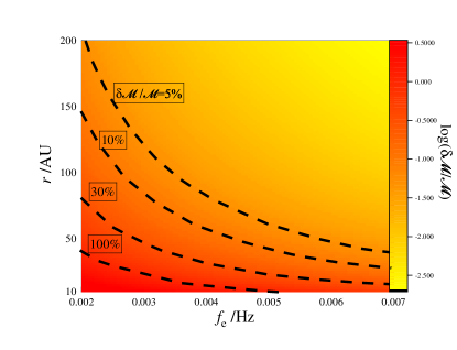
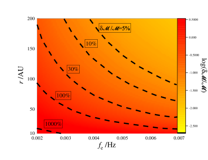
Figure 1: Bias of the chirp mass induced by the peculiar acceleration. The result is shown as a function of the GW frequency $f_{e}$ and the distance $r$ between the DWD and the tertiary star. The left panel corresponds to a stellar mass of $m_{3}=1\,M_{\odot}$ and the right one corresponds to $m_{3}=5\,M_{\odot}$. The dashed lines show the contours of different values of $\delta{\cal M}/{\cal M}$. In both cases, the chirp mass of the DWD is set to ${\cal M}=0.3\,M_{\odot}$. The outer orbit is circular and aligned with the line-of-sight.

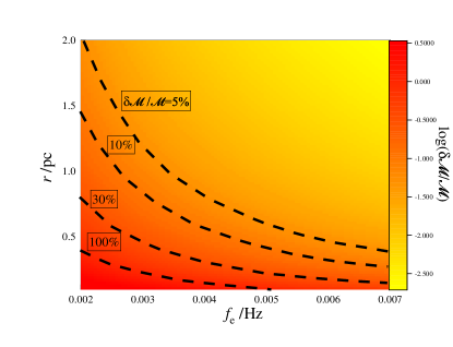
Figure 2: The same as Figure 1, but the tertiary is a SMBH with a mass of $4\times 10^{6}\,M_{\odot}$.

For the DWDs in the vicinity of the SMBH in the Galactic Center, the resulting bias is shown in Figure 2. We find a large parameter space in which the value of $\delta{\cal M}/{\cal M}$ exceeds $5\%$. In the lower-left corner of the diagram, the bias exceeds $100\%$ of ${\cal M}$. This is the region where the frequency shift due to peculiar acceleration greatly exceeds what is caused by GW radiation. Although not shown here, at a distance significantly smaller than $0.1$ pc, the bias could also exceed $10{\cal M}$.

We note that the DWDs presented in Figure 2 are dynamically stable. First, they are stable against the disruptive tidal force of the SMBH, since tidal disruption requires that

$$r\la 0.1\,{\rm{AU}}\,\left(\frac{m_{3}}{4\times 10^{6}\,M_{\odot}}\right)^{1/3}\left(\frac{f_{e}}{3\,\rm{mHz}}\right)^{-2/3},$$ (18)

where $4\times 10^{6}\,M_{\sun}$ is the mass of the SMBH in the Galactic Centre (Gillessen et al., 2009). Second, the secular interaction with the SMBH also induces a Lidov-Kozai evolution of the DWDs. However, the timescale is of the order of

$$T_{\rm{LK}}\sim 2\times 10^{10}{\rm{yr}}\left(\frac{m_{3}}{4\times 10^{6}M_{\odot}}\right)^{-1}\left(\frac{f_{e}}{3\rm{mHz}}\right)\left(\frac{r}{0.1\rm{pc}}\right)^{3}(1-e_{2}^{2})^{3/2},$$ (19)

where $e_{2}$ is the eccentricity of the orbit of the DWD around the SMBH (the outer orbit, see Naoz, 2016, for a review) and the mean value is about $0.67$ if the orbits of the DWDs are thermalized. Therefore, we can neglect the Lidov-Kozai effect during the observational period of four years of LISA. Equation (19) also indicates that the DWDs inside a radius of $0.1$ pc from the SMBH would have been depleted because the Lidov-Kozai effect could have driven them to merge. For this reason, we do not consider the DWDs with $r<0.1$ pc. Third, the specific internal kinetic energies of the DWDs are higher than the specific kinetic energies of the background stars by a factor of

$$\frac{Gm_{1}m_{2}}{(m_{1}+m_{2})a_{1}\sigma_{*}^{2}}=3\left(\frac{m_{1}}{0.34\,M_{\odot}}\right)^{2/3}\left(\frac{f_{e}}{3\,\rm{mHz}}\right)^{2/3}\left(\frac{\sigma_{*}}{200\,\rm{km}\,\rm{s}^{-1}}\right)^{-2},$$ (20)

where $\sigma_{*}$ denotes the velocity dispersion of the background stars. Such binaries are “hard”, so that they would not be ionized during the interactions with the surrounding stars (Binney & Tremaine, 1987).

3 Criterion for confusion

Now we study whether LISA could distinguish those DWDs affected by peculiar acceleration. Although an analytical criterion was provided in Robson et al. (2018), we derive a simplified version here for completeness, and for our later analysis of the population of DWDs in the Milky Way.

First, we note that the effect of peculiar acceleration is important only when the induced bias, $\delta{\cal M}$, is greater than the measurement error of chirp-mass, $\sigma_{\cal M}$. According to Equation 1, the variation of ${\cal M}$ is related to the variation of $\dot{f}_{e}$. For this reason, the condition $|\delta{\cal M}|<\sigma_{\cal M}$ is equivalent to $|\dot{f}_{o}-\dot{f}_{e}|<\Delta\dot{f}$, where $\Delta\dot{f}=6\sqrt{5}/\pi\cdot\rho^{-1}\tau_{\rm obs}^{-2}$ is the aforementioned threshold of detecting a frequency shift by LISA (Seto, 2002; Takahashi & Seto, 2002). Substituting Equation (8) for $\dot{f}_{o}$, we find that peculiar acceleration is not important when

$$r\ga 150\,{\rm{AU}}\,\left(\frac{\rho}{100}\right)^{1/2}\left(\frac{\tau_{\rm obs}}{4\,{\rm{yr}}}\right)\left(\frac{f_{e}}{3\,{\rm{mHz}}}\right)^{1/2}\left(\frac{m_{3}}{1\,M_{\odot}}\right)^{1/2},$$ (21)

where, again, we have neglected the higher-order terms of $\beta$, because of their smallness. For the DWDs in the Galactic Centre, the criterion becomes

$$r\ga 0.46\,{\rm{pc}}\,\left(\frac{\rho}{10}\right)^{1/2}\left(\frac{\tau_{\rm obs}}{4\,{\rm{yr}}}\right)\left(\frac{f_{e}}{3\,{\rm{mHz}}}\right)^{1/2}\left(\frac{m_{3}}{4\times 10^{6}\,M_{\odot}}\right)^{1/2}.$$ (22)

Second, so far we have assumed a more-or-less constant phase $\phi$ for the outer orbit. Such an approximation is valid when the observational period $\tau_{\rm obs}$ is much shorter than the orbital period of the tertiary $P_{3}$. In this case, we have shown that the peculiar acceleration contributes a constant term to $\dot{f}_{o}$ (the aforementioned $\dot{f}_{\rm acc}$). However, if the observational period is long, $\phi$ will sufficiently change so that $\dot{f}_{o}$ can no longer be regarded as a constant. In this case, the chirp signal is not a straight line in the $t-f_{o}$ diagram but curved. Figure 3 shows this effect. Detecting the curvature would allow us to distinguish accelerating DWDs from those not affected by peculiar acceleration.

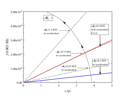
Figure 3: A curved chirp signal induced by the long-term effect of peculiar acceleration (red solid curve). It is distinguishable from the signals of those DWDs without acceleration (grey dashed lines). The blue solid line is the intrinsic chirp signal in the rest frame of the DWD. In this example, the tertiary has a mass of $m_{3}=1\,M_{\odot}$ and is at a distance of $r=20$ AU from the DWD. The corresponding orbital period $P_{3}$ is about $69$ years and the $\Gamma$ factor is about $3.4$. The orbital phase $\phi$ is chosen such that initially the acceleration effect maximizes.

Suppose the peculiar acceleration induces a second time derivative $\ddot{f}_{o}$. By definition, it is the curvature of the chirp signal. Detecting the curvature requires that $\ddot{f}_{\rm acc}\tau_{\rm obs}>\Delta\dot{f}$. From this relation and noticing that $\ddot{f}_{\rm acc}\tau_{\rm obs}\approx\dot{f}_{\rm acc}\tau_{\rm obs}/P_{3}$, we derive the criterion

$$r\la 26\,\rm{AU}\,\left(\frac{\rho}{100}\right)^{2/7}\left(\frac{\tau_{\rm obs}}{4\,\rm{yr}}\right)^{6/7}\left(\frac{f_{e}}{3\,\rm{mHz}}\right)^{2/7}\left(\frac{m_{3}}{1\,M_{\odot}}\right)^{3/7}.$$ (23)

This criterion can also be derived using Equations (32), (A9) and (A10) in Robson et al. (2018). There is another way of understanding Equation (23). Given $f_{e}$, $r$, $m_{3}$ and $\rho$, solving for $\tau_{\rm obs}$ would yield a minimal observational time, which we call $T_{\rm cri}$. This is the shortest observational time that is needed to detect the effect of peculiar acceleration.

For the DWDs in the Galactic Centre, the criterion of distinguishing the peculiar acceleration becomes

$$r\la 0.044\,\rm{pc}\,\left(\frac{\rho}{10}\right)^{2/7}\left(\frac{\tau_{\rm obs}}{4\,\rm{yr}}\right)^{6/7}\left(\frac{f_{e}}{3\rm{mHz}}\right)^{2/7}\left(\frac{m_{3}}{4\times 10^{6}M_{\odot}}\right)^{3/7}.$$ (24)

We have mentioned in the previous section that the mass bias could be as large as $10{\cal M}$ if a DWD is within a distance of $0.1$ pc from the SMBH in the Galactic Centre. Now we can further predict that the peculiar acceleration is undetectable if the distance is also greater than about $0.05$ pc. In this case, the DWD could be mis-identified as a DNS or BBH, or even a lower-mass-gap object (also see Table 1 of Chen, 2020).

Figure 4 shows the regions in the parameter space of $m_{3}$ and $r$ where the effect of peculiar acceleration is unimportant ($\delta{\cal M}<\sigma_{\cal M}$) or large enough to be detectable within an observational period of $4$ years ($T_{\rm cri}<4$ years).

In general, wider triple systems with lighter tertiary stars are less affected by peculiar acceleration, and more compact triples with heavier tertiaries are more likely to reveal the signatures of peculiar acceleration. Outside the hatched region, the effect of peculiar acceleration is strong but difficult to discern. Here the DWDs are likely to cause confusion. The measurement of their masses and distances could be significantly biased.

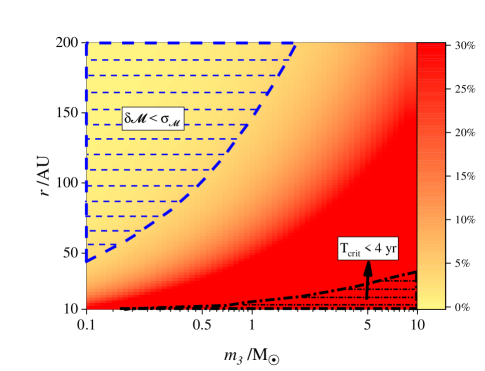
Figure 4: The $m_{3}-r$ parameter space where the effect of peculiar acceleration is unimportant (top-left hatched region labeled with $\delta{\cal M}<\sigma_{\cal M}$) or large enough to be detectable within an observational period of $4$ years (bottom-right hatched region labeled with $T_{\rm cri}<4$ years). The background color encodes the value of $\delta\mathcal{M}/\mathcal{M}$. We have assumed a canonical observational scenario where $f_{e}=3$ mHz, $\tau_{\rm obs}=4$ years and $\rho=100$.

Figure 5 shows the location of the confusing DWDs in the parameter space of $f_{e}$ and $r$. Note that the confusing DWDs reside outside the hatched regions. In the plot we have assumed that $m_{3}=1\,M_{\odot}$. In this case, the critical distance where confusion starts to occur is insensitive to the GW frequency. Therefore, we find a large area above $r\ga 10$ AU where the measured ${\cal M}_{o}$ and $d_{o}$ would be biased.

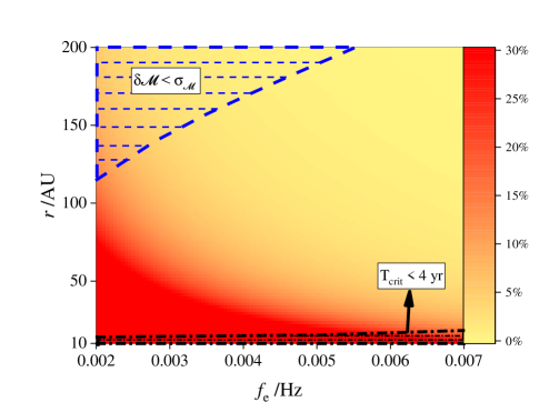
Figure 5: The same as Figure 4 but showing the results in the parameter space of $f_{e}$ and $r$. The mass of the tertiary is $m_{3}=1M_{\sun}$.

For the DWDs around the SMBH in the Galactic Centre, the result is shown in Figure 6. The region where the peculiar acceleration is detectable ($T_{\rm cri}<4$) disappears. This is because in the radial range of our interest, $r>0.1$ pc, the outer orbital period is much longer than the observational period. In this case, the curvature of the chirp signal is undetectable during the four years of LISA mission. Therefore, the mass is completely degenerate with the peculiar acceleration for these DWDs in the Galactic Centre.

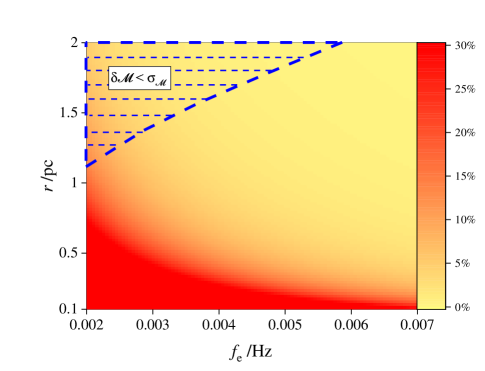
Figure 6: Similar to Figure 5 but assuming a tertiary of a mass of $m_{3}=4\times 10^{6}\,M_{\odot}$. The region where $T_{\rm cri}<4$ years is at a radius smaller than $r=0.1$ pc, and hence not shown in the plot.

4 Numerical verification

Now we verify the analytical results presented in the previous two sections using a numerical technique called “matched filtering” (Finn, 1992; Cutler & Flanagan, 1994). It is commonly employed in GW data analysis to estimate the physical parameters of the source. For our purpose, we use this technique to evaluate the similarity between the waveform of an accelerating DWD and the waveform of a non-moving DWD but with a different chirp mass. To differentiate the two waveforms, we denote the previous one as $h_{1}$ and the latter one as $h_{2}$.

The similarity between $h_{1}$ and $h_{2}$ can be quantified by a “fitting factor” ($\rm FF$), defined as

$$\mathrm{FF}\equiv\frac{\left\langle h_{1}|h_{2}\right\rangle}{\sqrt{\left\langle h_{1}|h_{1}\right\rangle\left\langle h_{2}|h_{2}\right\rangle}},$$ (25)

where $\left\langle h_{1}|h_{2}\right\rangle$ denotes the inner product of the two waveforms, which can be computed with

$$\left\langle h_{1}|h_{2}\right\rangle=2\int_{0}^{\infty}\frac{\tilde{h}_{1}(f)\tilde{h}_{2}^{*}(f)+\tilde{h}_{1}^{*}(f)\tilde{h}_{2}(f)}{S_{\rm{n}}(f)}{\rm{d}}f.$$ (26)

In the last equation, the tilde symbol means a Fourier transformation of the waveform, the star stands for the complex conjugate and $S_{n}(f)$ is the spectral noise density of LISA (N2A5 configuration including a DWD background, Klein et al., 2016). A perfect match between the two waveforms would yield ${\rm FF}=1$.

As is shown in Chen & Shen (2019); Chen et al. (2020), the calculation of ${\rm FF}$ can be performed in the time domain when the chirp rate $\dot{f}_{o}$ is relatively small. When $\dot{f}_{o}\tau_{\rm obs}\ll f_{o}$, which is the case for our DWDs, we can use the Parseval’s theorem and write

$$\left\langle h_{1}|h_{2}\right\rangle\approx\frac{4}{S_{n}(f)}\int_{0}^{\infty}h_{1}(t)h_{2}(t){\rm{d}}t.$$ (27)

Consequently,

$$\mathrm{FF}=\frac{\int_{0}^{\infty}h_{1}(t)h_{2}(t){\rm{d}}t}{\sqrt{\int_{0}^{\infty}h_{1}(t)h_{1}(t){\rm{d}}t\int_{0}^{\infty}h_{2}(t)h_{2}(t){\rm{d}}t}}.$$ (28)

Computing the inner product in the time domain significantly simplifies and accelerates our calculation.

Having defined the FF, we can use it to determine the bias $\delta{\cal M}$ induced by peculiar acceleration. The steps are as follows. (1) Given the chirp mass ${\cal M}$ and GW frequency $f_{e}$ of a DWD, we compute the waveform in the rest frame of the binary using a 3.5 post-Newtonian approximation presented in (Sathyaprakash & Schutz, 2009). Although this approximation is derived for test particles, it is appropriate for our DWDs because in the mHz band the tidal interaction between the white dwarfs (WDs) are negligible (Kremer et al., 2017). (2) We specify the mass and distance of the tertiary, and add the effected of the peculiar acceleration to the waveform according to Equation (8). Such a modified waveform, as is mentioned before, is our $h_{1}$. (3) We generate a suite of waveforms for non-moving DWDs with different chirp masses ${\cal M}^{\prime}$. These waveform templates are our $h_{2}$. (4) We search for the maximum FF between $h_{1}$ and $h_{2}$. The ${\cal M}^{\prime}$ corresponds to the best fit is the apparent chirp mass, ${\cal M}_{o}$. (5) The bias is then the difference between the intrinsic ${\cal M}$ and the observed ${\cal M}_{o}$.

Figure 7 shows an example of the bias found by the matched-filtering scheme. Comparing it with the analytical result shown in the left panel of Figure 1, we find no apparent difference. By comparing the left and right panels in Figure 7, we also find that the bias is insensitive to the observational period. Therefore, we are justified to use the analytical formulae presented in Section 2 to calculate the mass bias $\delta{\cal M}$.

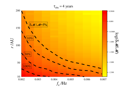
Figure 7: The mass bias found by the matched-filtering method. In the left panel, the length of the waveforms is $2.5$ years, and in the right one the length is $4$ years. The other parameters are the same as in the left panel of Figure 1.

Next, we use the matched-filtering method to test our Equation (23). A DWD not satisfying this equation is expected to cause confusion and leads to an wrong estimation of its chirp mass. In the context of matched filtering, the condition of confusing two waveforms of different origin is

$$\mathrm{FF}>1-1/(2\rho^{2}).$$ (29)

This criterion was suggested by Lindblom et al. (2008) and has been used in our earlier works Chen & Shen (2019); Chen et al. (2020). For the purpose of this work, $h_{1}$ is the waveform of an accelerating DWD and $h_{2}$ the waveform of a non-moving DWD. The criterion to confuse $h_{1}$ and $h_{2}$ would be $\rm FF>0.99995$ if we adopt our fiducial SNR $\rho=100$.

Figure 8 shows the mass bias (upper panel) and the corresponding FF derived from the matched filtering method (lower panel). The other models parameters are $f_{e}=3$ mHz, ${\cal M}=0.3\,M_{\odot}$, and $m_{3}=1\,M_{\odot}$. To simplify the problem, we assume that the orbit of the tertiary is circular and the inclination is $i=0$. Initially, the orbital phase $\phi$ is set to a value that maximizes the mass bias. For comparison, our analytical criterion is shown as the grey dashed line. We find that the analytical and numerical criteria agree well at $r\la 15$ AU. At $r\ga 30$ AU, both results are also consistent, suggesting that ${\rm FF}\simeq 1$ and LISA might confuse an accelerating DWD with a non-moving one with a different chirp mass. The difference between the analytical and numerical criteria is large between $r=15$ and $30$ AU. Nevertheless, no DWD below the dashed line has a FF lower than $0.99997$, suggesting that the analytical criterion is more stringent than the numerical one. In the following we will use the analytical criterion, calibrated by our numerical matched-filtering results, to select the DWDs which might cause confusion.

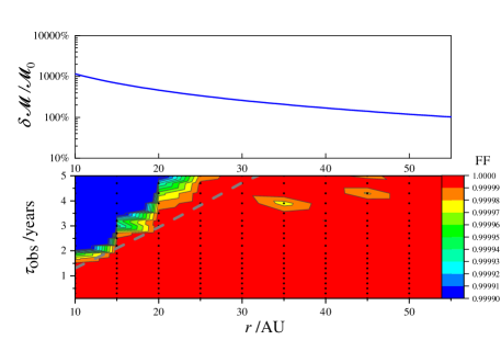
Figure 8: Upper panel: The mass bias found by the matched-filtering method as a function of the distance of the tertiary. Lower panel: Dependence of the FF on the distance of the tertiary and the observational period. The grey dashed line is computed using Equation (23). The black dots mark the grids where we performed parameter estimation using the matched-filtering method.

5 Population synthesis model

Having understood the effect of peculiar acceleration on the measurement of the mass and distance of DWDs, we can now proceed to study how many DWDs in the LISA band would be substantially affected. In the following, we will focus on the DWDs with stellar-mass companions because they are more common than those in the Galactic Centre around the SMBH.

We note that our current understanding of the DWD population in triples is limited, mainly due to the observational challenges of detecting companions within a distance of about $100$ AU from DWDs (Arenou et al., 2018; Hallakoun & Maoz, 2019). However, observations of isolated DWDs and main-sequence multiples are relatively rich. Therefore, we will use the information provided by the latter observations to infer the statistical properties of the DWDs in triples. Given the uncertainties, it is not our desire to build a comprehensive model for triple-star evolution. Instead, we start from the recent theoretical results of isolated DWDs and investigate the effect of tertiaries on the measurement of their masses and distances. Our model can be divided into the following three parts.

First, we use a Monte-Carlo code to generate a population of DWDs in the mHz band. The method is based on the distribution functions presented in Lamberts et al. (2019), which include the intrinsic chirp mass ${\cal M}$, mass ratio $q:=m_{2}/m_{1}$, GW frequency $f_{e}$ and the real heliocentric distance $d$ to the sun. The initial sample contains $330,000$ DWDs. We then select from them the binaries with a high SNR, $\rho>8$, assuming an observational period of $4$ years by LISA. It results in about $10,340$ DWDs in the frequency band of $10^{-2}-10$ mHz. The majority of these high-SNR binaries fall in the frequency band $1-10$ mHz. We also recover the result of Lamberts et al. (2019), that during the four-year mission of LISA about $12,000$ DWDs can be individually resolved because of their high SNRs.

Second, we determine whether the $10^{4}$ DWDs generated in the previous step have tertiaries. This is done using the results of the bifurcation model presented in Eggleton (2009). This model divides a stellar system with a given total mass into smaller and smaller sub-systems, a process called “bifurcation”. Each step of bifurcation follows a probability which is derived from the stellar multiples observed by the Hipparcos satellite. The probability is a function of the bifurcation level and the mass of the system to be divided. In general, higher bifurcation levels and smaller masses lead to lower probability for further bifurcation. More details can be found in the Equations (8), (17)-(20) and Table 2 in Eggleton (2009).

Following the bifurcation model, we generate a sample of about $2\times 10^{7}$ binary and triple main-sequence stars. The sample size is far less than the real number of binaries and triples in the Milky Way, but large enough for our purpose, i.e., deriving the probability that a DWD generated in the first step has a tertiary companion. Not all of the $2\times 10^{7}$ stellar multiples can produce close DWDs in the LISA band. Therefore, we apply two more criteria to find the systems which could yield LISA DWDs. (1) The stellar components of the binaries (including the inner binaries in the triples) fall in the mass range of $0.9M_{\odot}\sim 8M_{\odot}$. This criterion ensures that the main-sequence binaries eventually evolve into DWDs. It is based on the empirical relationship

$$M_{\rm{core}}=0.1\left(M_{\rm{MS}}/M_{\odot}\right)^{1.4}$$ (30)

between the mass of the progenitor star $M_{\rm{MS}}$ and the mass of the stellar core $M_{\rm{core}}$ (Postnov & Yungelson, 2014). (2) The orbital periods of the main-sequence binaries (including the inner binaries) fall in the range between $0.1$ day and $1$ year. This requirement comes from the fact that for a binary star with a total mass of about $2\,M_{\odot}$, the orbital semimajor axis typically shrinks by a factor of $100$ during the later common-envelope phases (Postnov & Yungelson, 2014; Hamers et al., 2013; Woods et al., 2012). In this case, an initial orbital period of $10^{-3}-1$ year would lead to a final orbital frequency bewteen $10^{-2}$ and $10$ mHz. By applying the above two selection criteria, we have about $10^{5}$ systems left. About $36\%$ are binaries and $64\%$ are triples. This result is also consistent with the observational result that the binaries with shorter orbital periods are more likely in triples (Pribulla & Rucinski, 2006; Tokovinin et al., 2008). Based on these results, we randomly select $6,400$ DWDs from the previous sample of $10,340$ and assume that they have tertiaries.

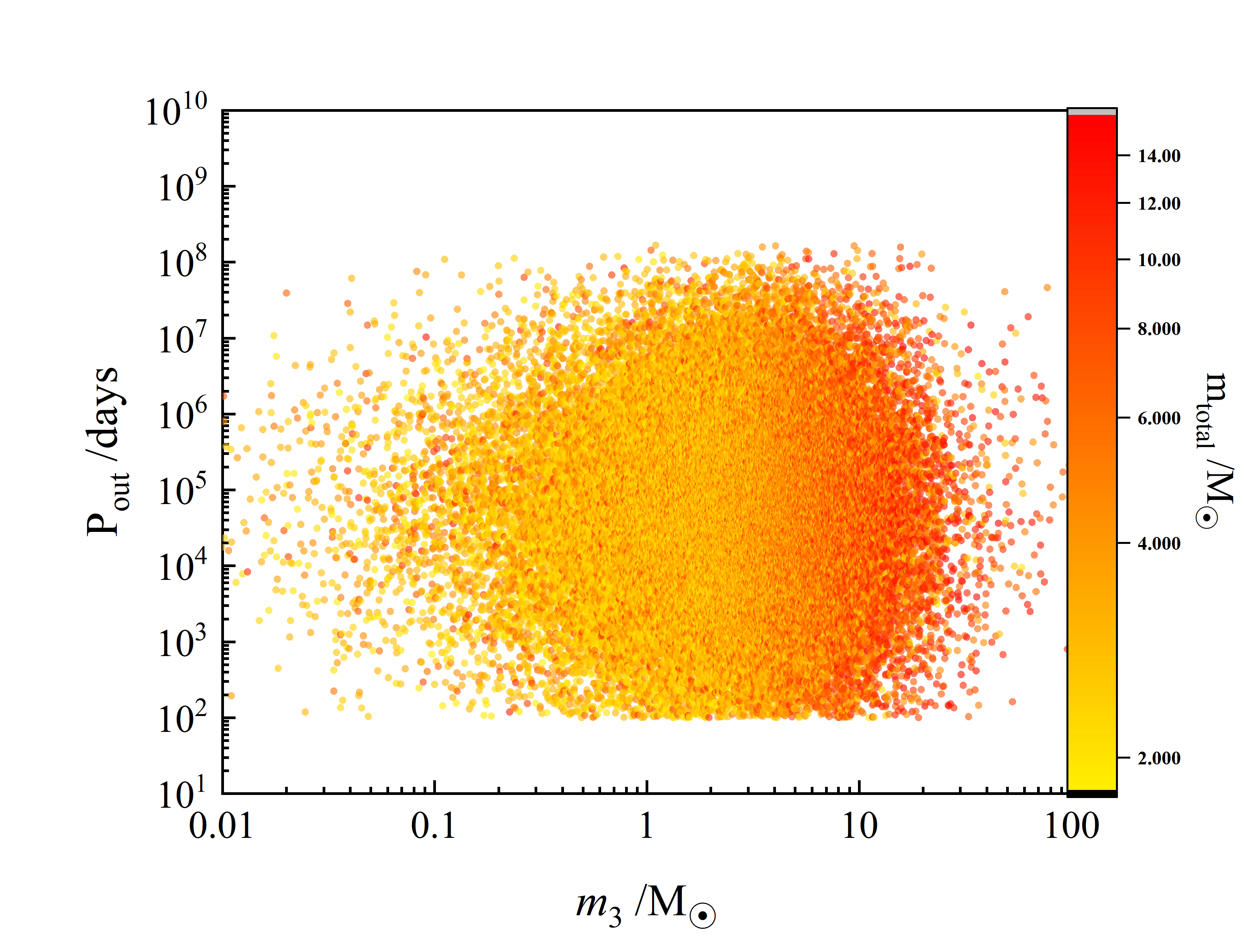
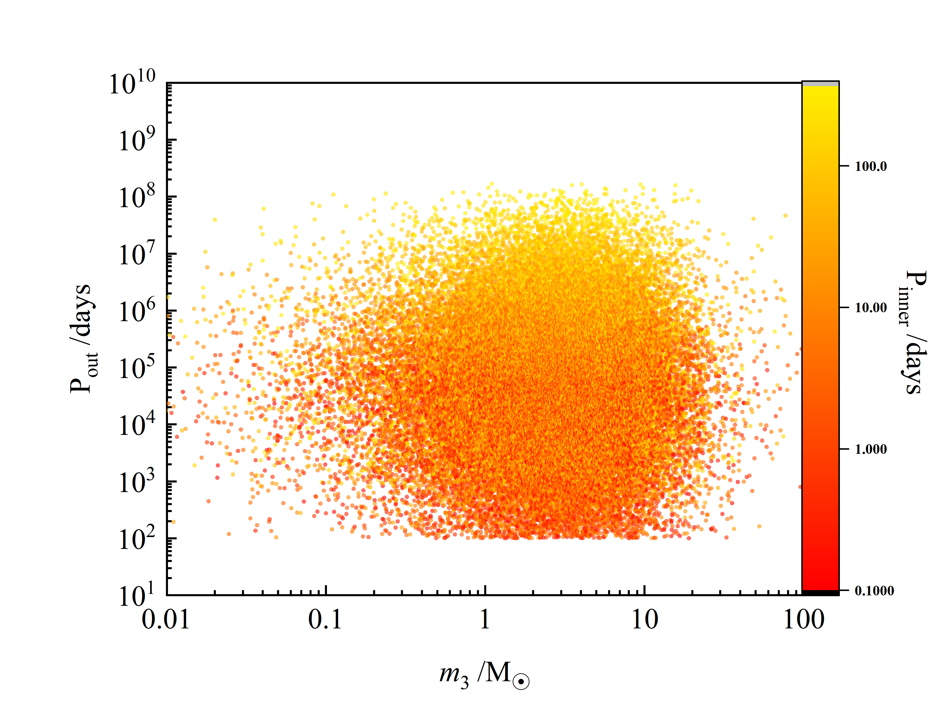
Figure 9: Distribution of the $6.4\times 10^{4}$ triple main-sequence stars which will produce DWDs in the LISA band. Here $m_{3}$ is the initial mass of the tertiary star and $P_{\rm out}$ stands for the initial orbital period of the outer binary. In the left panel the color indicates the total mass $m_{\rm total}$ of the inner main-sequence binary, and in the right panel the color stands for the initial orbital period of the inner binary.

Third, for each of the $6,400$ selected DWDs with tertiaries, we determine the mass and distance of the third star. This is done in two steps. (1) Given a DWD with a tertiary, we identify the progenitor triple based on the $6.4\times 10^{4}$ triple stars from our bifurcation model. The distribution of the $6.4\times 10^{4}$ triples is shown in Figure 9. We find that tertiaries are more likely to appear for heavier binaries (left panel) and their orbital periods are closely correlated with the orbital periods of the inner binaries (right panel). Because of these correlations, the mass and distance of a tertiary should not be selected randomly. In our model, the progenitor triple is identified according to the masses of the binary components and the relationship given by Equation (30). Sometimes more than one progenitor triple can be found for a DWD with a tertiary. In these cases, we randomly select one progenitor. (2) Having found the progenitor triples, we evolve the outer orbits according to the ages of the $6,400$ DWDs. The age of the DWD is randomly selected between the age of the progenitor stars, $10\,(M_{\rm MS}/M_{\odot})^{-3}$ Gyr (Kippenhahn & Weigert, 1994), and the age of the Galaxy, $13.7$ Gyr. The evolution of the outer triple is caused by the mass loss of the progenitors stars during their post-main-sequence evolution, and we use the equation for adiabatic orbital expansion,

$$\frac{r(\rm{now})}{r(\rm{initial})}=\frac{m_{1}+m_{2}+m_{3}+\Delta m}{m_{1}+m_{2}+m_{3}}$$ (31)

(Toonen et al., 2016), to find the current distance of the tertiary. The amount of mass loss, $\Delta m$, can be calculated using the relationship given by Equation (30). Note that if the age of the DWD exceeds the main-sequence lifetime of the tertiary star, the tertiary also loses mass and evolves into a compact object. In this case, we add the mass loss to $\Delta m$ and update $m_{3}$ according to Equation (30).

6 Mock LISA observation

So far we have generated a sample of about $10^{4}$ DWDs in the LISA band, whose masses, heliocentric distances and GW frequencies follow the distributions given in Lamberts et al. (2019). The difference of our sample is that about $64\%$ of them are in triple systems, and we have determined the masses and distances of the tertiaries.

Then we check whether LISA could detect the chirp signals of these $10^{4}$ DWDs. We first calculate the GW amplitude in the frequency domain for each DWD (following Seto, 2002) and use Equation (26) to compute the SNR ($\rho$). A canonical observational period of $\tau_{\rm obs}=4$ years is assumed. For those isolated DWDs, which constitute $36\%$ of the sample, we use Equation (4) to select the ones with detectable chirp signals. For the rest $64\%$, which are triples, we use the criterion $|\dot{f}_{o}|>\Delta\dot{f}$ to take into account the effect of peculiar acceleration. In the end, we have $8105$ DWDs whose chirping rate is resolvable by LISA. We note that this number is about eight times larger than the number of DWDs with measured mass given in Lamberts et al. (2019), because they used a more strict requirement that the chirp mass should be measured to an accuracy of $10\%$.

For these $8,105$ DWDs, we calculate their apparent chirp masses and apparent distances using Equations (11), (12) and (16), so that we can evaluate the biases relative to the real masses and real distances. In the calculation, for each triple system we have assumed a random distribution for the inclination ($i$) and phase ($\phi$) of the outer orbit, so that the effect of peculiar acceleration is, on average, weaker than what is predicted by Equation (16). We also apply Equation (23) to judge whether we would confuse the DWD in a triple and an isolated DWD with a different chirp mass.

Figure 10 shows the real chirp mass and frequency (left panel) of the $8,105$ DWDs and the observed values (right panel). Comparing the two panels, we find that the majority of the DWDs are not significantly affected by the presence of tertiaries (yellow dots). The DWDs most affected by peculiar acceleration (red dots) are those with relatively low GW frequencies, e.g., below $4$ mHz. Most of them are indistinguishable from isolated, non-moving DWDs. For these confusing DWDs, the intrinsic chirp rate $\dot{f}_{e}$ is small, so that it can be overcome by the additional chirp rate $\dot{f}_{\rm{acc}}$ induced by peculiar acceleration. Moreover, we find from the right panel that at higher frequencies there are less red dots but more blue ones. This trend indicates that at high frequencies, it is difficult for a tertiary to induce a large mass bias in a DWD and at the same time keep the accelerating DWD indistinguishable from isolated, non-moving DWDs. This is so because higher frequency corresponds to larger $\dot{f}_{\rm{GW}}$, so that the tertiary should get closer to the DWD to induce a significant mass bias. As the tertiary gets closer, the period of the outer orbit shortens and the curvature of the chirp signal becomes more prominent.

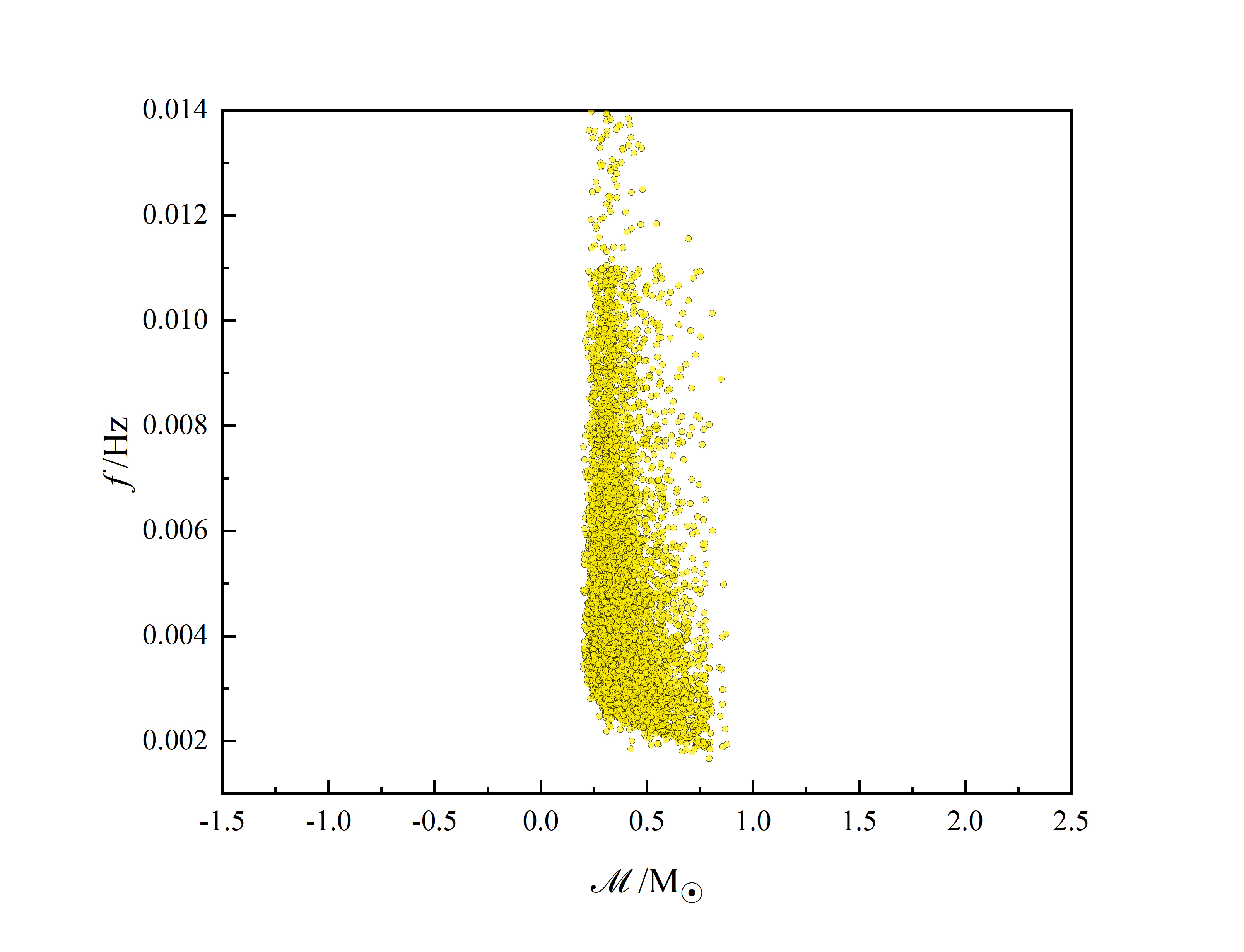
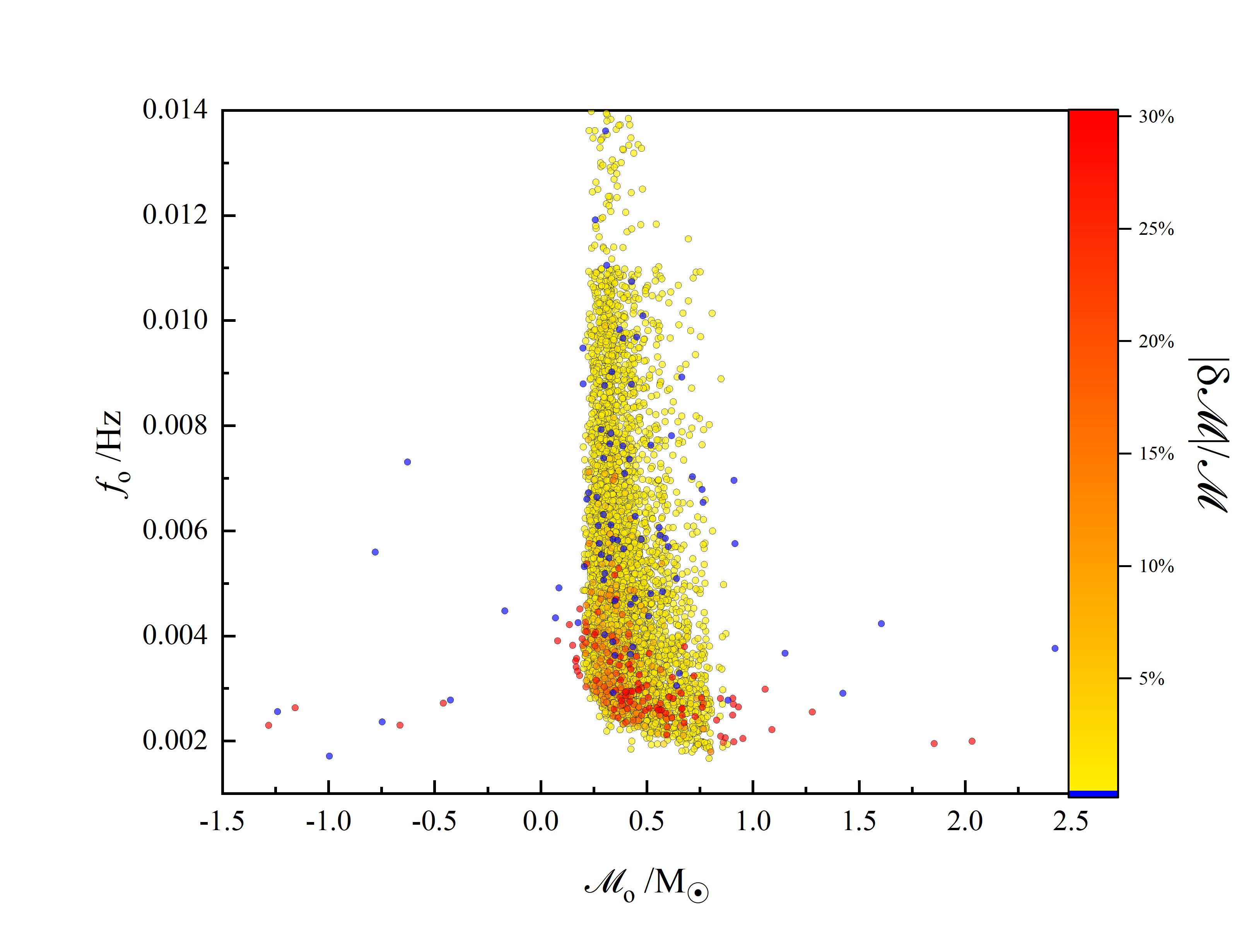
Figure 10: Left panel: The intrinsic chirp masses and GW frequencies of the $8105$ DWDs whose chirping rate can be resolved by LISA. Right panel: The apparent chirp masses and GW frequencies of the same DWDs, color-coded by the mass bias. The blue dots are the DWDs with a distinguishable peculiar acceleration. Several DWDs have negative chirp masses because the $\Gamma$ factor becomes smaller than $-1$.

Several confusing DWDs (red dots) in the right panel of Figure 10 are worth mentioning.

• One red dot appears at ${\cal M}_{o}>2.0\,M_{\odot}$ with a SNR of $8.6$. Therefore, it looks like a DNS, e.g., $m_{1}=m_{2}=2.3\,M_{\odot}$, or even a binary containing a lower-mass-gap object, e.g., $m_{1}=4\,M_{\odot}$ and $m_{2}=1.4\,M_{\odot}$. In fact, the real chirp mass is only $0.39\,M_{\odot}$. The apparent chirp rate is raised by a tertiary stellar-mass black hole of a mass of $7.4\,M_{\odot}$ orbiting at a distance of $22$ AU from the DWD. The real heliocentric distance of this system is about $8.4$ kpc, but due to the peculiar acceleration, it appears to be at a distance of $130$ kpc.

• Less extreme cases can be found at ${\cal M}_{o}\simeq 1\,M_{\odot}$. For example, one red dot appears at ${\cal M}_{o}\simeq 1.28\,M_{\odot}$ with a SNR of $12$, so that it looks like a DNS. The real chirp mass is actually $0.35\,M_{\odot}$. The tertiary is a compact object at a distance of $14$ AU and has a mass of $1.4\,M_{\odot}$. Therefore, it is either a high-mass WD or a low-mass neutron star. The real heliocentric distance is about $14$ kpc, but it appears to be at $d_{o}\simeq 126$ kpc because of the peculiar acceleration.

• There are $11$ red dots with a chirp mass significantly smaller than $0.2\,M_{\odot}$. Theoretically, such small compact-object binaries are difficult to form. In fact, their real chirp masses are about $0.3\,M_{\odot}$. The tertiaries include main-sequence stars, neutron stars and black holes. The most extreme one has an apparent chirp mass of ${\cal M}_{o}\simeq 0.079\,M_{\odot}$ with a SNR of $46$. Such a system could be misidentified as a binary of primordial black holes. Its real chirp mass is $0.29\,M_{\odot}$, and the tertiary is a black hole of $3.5\,M_{\odot}$ orbiting at a distance of $35$ AU. The real heliocentric distance is $5.6$ kpc, but because of the peculiar acceleration, it appears closer, at about $d_{o}\simeq 650$ pc.

• We also find red dots with negative chirp masses. They are caused by the fact that $\dot{f}_{\rm acc}$, and hence the total $\dot{f}_{o}$, can both be negative. The signal with a negative chirp rate is known as “inverse chirp”. In the conventional model of DWD, such a signal can be produced by a mass transfer between the two WDs (Nelemans et al., 2004). Because of this possibility, it is difficult to distinguish these red dots with ${\cal M}_{o}<0$ from the DWDs undergoing mass transfer. We note that most of these confusing DWDs have black-hole or neutron-star tertiaries.

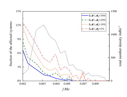
Figure 11: The fraction of confusing DWDs in each frequency bin (colored curves). The red, orange, green and blue lines, respectively, refer to the DWDs with a mass bias greater than $5$, $10$, $20$ and $30$ per cent. For reference, the black dotted line shows the distribution of all the DWDs with measurable chirp masses.

Among these $8,105$ DWDs of which we can derive chirp masses, $75,\,144,\,193,\,319$ have a mass bias greater than $30,\,20,\,10,\,5$ per cent and at the same time they are indistinguishable from isolated DWDs. Therefore, confusing DWDs constitute about $9\%$ of the LISA DWDs with measurable masses. Figure 11 shows more clearly the distribution of these confusing DWDs in the frequency space. We find that in general there is a larger fraction of confusing DWDs at lower frequencies. This result can be understood since the chirp rate due to GW radiation drops as the frequency decreases.

We have shown in Section 2 that bias in the measurement of chirp mass will also result in a bias in the measured distance. Figure 12 shows this effect using the $8,105$ simulated DWDs. Comparing the red and blue curves, we find an significant excess of binaries at a relatively low distance, below $1$ kpc, when triples and the resulting peculiar acceleration are taken into account. Since these additional binaries are fake and their real distances are much larger than the apparent ones, it would be impossible for future deep photometric surveys, such as LSST and Gaia (e.g. Korol et al., 2019), to find their electro-magnetic counterparts. Moreover, Figure 12 also shows that there are binaries in the LISA band which appear to be beyond $100$ kpc. They are also fake since the real distance (blue curve) stops at $100$ kpc. These results highlight the potential problem that the DWDs in triples may bring to our understanding of the Galactic structure.

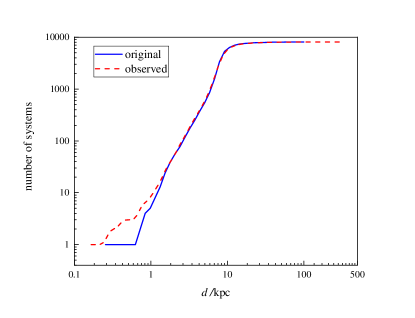
Figure 12: Cumulative distribution of the real (blue solid line) and observed (red dashed line) distances for the $8\times 10^{3}$ DWDs with measurable chirp masses.

7 Summary and conclusion

In this work, we have demonstrated the effect of peculiar acceleration induced by tertiaries on the measurement of the mass and distance of the DWDs in the LISA band. Different from the previous works, our method is mainly analytical, but we also verify the key results using numerical simulations. Using the analytical results, we are able to conduct mock LISA observation of a large population of simulated DWDs with tertiaries.

We find that about $9\%$ of the DWDs of which LISA can measure a chirp mass are affected by peculiar acceleration. They reside mostly in the frequency band of $2-4$ mHz and are indistinguishable from isolated, non-moving DWDs. The bias in the mass measurement is mostly $(5-30)\%$, but there are also cases in which the bias exceeds $100\%$. In those extreme cases, the DWDs can mimic DNSs, BBHs, DWDs undergoing mass transfer, or even binaries containing lower-mass-gap objects and primordial black holes. As a result of the bias, the distance of the DWDs measured by LISA are also inaccurate. It leads to an apparent over-population of DWDs within a heliocentric distance of $1$ kpc as well as beyond $100$ kpc.

In general, our results highlight the importance of modeling the astrophysical environments of GW sources (e.g. Chen, 2020). For DWDs, in particular, developing population synthesis models for triple stars is necessary and urgently needed.

References

- Adams et al. (2012) Adams M. R., Cornish N. J., Littenberg T. B., 2012, Phys. Rev. D, 86, 124032
- Amaro-Seoane et al. (2017) Amaro-Seoane P., et al., 2017, arXiv e-prints, p. arXiv:1702.00786
- Arenou et al. (2018) Arenou F., et al., 2018, A&A, 616, A17
- Binney & Tremaine (1987) Binney J., Tremaine S., 1987, Galactic dynamics. Princton University Press
- Bonvin et al. (2017) Bonvin C., Caprini C., Sturani R., Tamanini N., 2017, Phys. Rev. D, 95, 044029
- Breivik et al. (2020) Breivik K., Mingarelli C. M. F., Larson S. L., 2020, ApJ, 901, 4
- Broadhurst et al. (2018) Broadhurst T., Diego J. M., Smoot George I., 2018, arXiv e-prints, p. arXiv:1802.05273
- Caputo et al. (2020) Caputo A., Sberna L., Toubiana A., Babak S., Barausse E., Marsat S., Pani P., 2020, ApJ, 892, 90
- Chen (2020) Chen X., 2020, arXiv e-prints, p. arXiv:2009.07626
- Chen & Shen (2019) Chen X., Shen Z., 2019, Proceedings, 17, 4
- Chen et al. (2019) Chen X., Li S., Cao Z., 2019, MNRAS, 485, L141
- Chen et al. (2020) Chen X., Xuan Z.-Y., Peng P., 2020, ApJ, 896, 171
- Cooray & Seto (2005) Cooray A., Seto N., 2005, ApJ, 623, L113
- Cutler & Flanagan (1994) Cutler C., Flanagan É. E., 1994, Phys. Rev. D, 49, 2658
- Deme et al. (2020) Deme B., Hoang B.-M., Naoz S., Kocsis B., 2020, The Astrophysical Journal, 901, 125
- Eggleton (2009) Eggleton P. P., 2009, MNRAS, 399, 1471
- Farr et al. (2011) Farr W. M., Sravan N., Cantrell A., Kreidberg L., Bailyn C. D., Mandel I., Kalogera V., 2011, ApJ, 741, 103
- Finn (1992) Finn L. S., 1992, Phys. Rev. D, 46, 5236
- Gillessen et al. (2009) Gillessen S., Eisenhauer F., Trippe S., Alexand er T., Genzel R., Martins F., Ott T., 2009, ApJ, 692, 1075
- Hallakoun & Maoz (2019) Hallakoun N., Maoz D., 2019, MNRAS, 490, 657
- Hamers et al. (2013) Hamers A. S., Pols O. R., Claeys J. S. W., Nelemans G., 2013, MNRAS, 430, 2262
- Inayoshi et al. (2017) Inayoshi K., Tamanini N., Caprini C., Haiman Z., 2017, Phys. Rev. D, 96, 063014
- Kippenhahn & Weigert (1994) Kippenhahn R., Weigert A., 1994, Stellar Structure and Evolution. Springer-Verlag, Berlin
- Klein et al. (2016) Klein A., et al., 2016, Phys. Rev. D, 93, 024003
- Korol et al. (2019) Korol V., Rossi E. M., Barausse E., 2019, MNRAS, 483, 5518
- Kremer et al. (2017) Kremer K., Breivik K., Larson S. L., Kalogera V., 2017, ApJ, 846, 95
- LIGO Scientific Collaboration & Virgo Collaboration (2019) LIGO Scientific Collaboration Virgo Collaboration 2019, ApJ, 882, L24
- Lagos et al. (2020) Lagos F., Schreiber M. R., Parsons S. G., Gänsicke B. T., Godoy N., 2020, MNRAS, 499, L121
- Lamberts et al. (2019) Lamberts A., Blunt S., Littenberg T. B., Garrison-Kimmel S., Kupfer T., Sanderson R. E., 2019, MNRAS, 490, 5888
- Lindblom et al. (2008) Lindblom L., Owen B. J., Brown D. A., 2008, Phys. Rev. D, 78, 124020
- Meiron et al. (2017) Meiron Y., Kocsis B., Loeb A., 2017, ApJ, 834, 200
- Naoz (2016) Naoz S., 2016, ARA&A, 54, 441
- Nelemans et al. (2001) Nelemans G., Yungelson L. R., Portegies Zwart S. F., 2001, A&A, 375, 890
- Nelemans et al. (2004) Nelemans G., Yungelson L. R., Portegies Zwart S. F., 2004, MNRAS, 349, 181
- Özel et al. (2010) Özel F., Psaltis D., Narayan R., McClintock J. E., 2010, ApJ, 725, 1918
- Perpinyà-Vallès et al. (2019) Perpinyà-Vallès M., Rebassa-Mansergas A., Gänsicke B. T., Toonen S., Hermes J. J., Gentile Fusillo N. P., Tremblay P. E., 2019, MNRAS, 483, 901
- Pfuhl et al. (2014) Pfuhl O., Alexander T., Gillessen S., Martins F., Genzel R., Eisenhauer F., Fritz T. K., Ott T., 2014, ApJ, 782, 101
- Postnov & Yungelson (2014) Postnov K. A., Yungelson L. R., 2014, Living Reviews in Relativity, 17, 3
- Pribulla & Rucinski (2006) Pribulla T., Rucinski S. M., 2006, AJ, 131, 2986
- Randall & Xianyu (2019) Randall L., Xianyu Z.-Z., 2019, ApJ, 878, 75
- Robson et al. (2018) Robson T., Cornish N. J., Tamanini N., Toonen S., 2018, Phys. Rev. D, 98, 064012
- Sathyaprakash & Schutz (2009) Sathyaprakash B. S., Schutz B. F., 2009, Living Reviews in Relativity, 12, 2
- Seto (2002) Seto N., 2002, MNRAS, 333, 469
- Seto (2008) Seto N., 2008, ApJ, 677, L55
- Smith et al. (2018) Smith G. P., Jauzac M., Veitch J., Farr W. M., Massey R., Richard J., 2018, MNRAS, 475, 3823
- Steffen et al. (2018) Steffen J. H., Wu D.-H., Larson S. L., 2018, arXiv e-prints, p. arXiv:1812.03438
- Stephan et al. (2019) Stephan A. P., et al., 2019, ApJ, 878, 58
- Takahashi & Seto (2002) Takahashi R., Seto N., 2002, ApJ, 575, 1030
- Tamanini & Danielski (2019) Tamanini N., Danielski C., 2019, Nature Astronomy, 3, 858
- Tamanini et al. (2020) Tamanini N., Klein A., Bonvin C., Barausse E., Caprini C., 2020, Phys. Rev. D, 101, 063002
- Tokovinin et al. (2008) Tokovinin A., Thomas S., Sterzik M., Udry S., 2008, in Hubrig S., Petr-Gotzens M., Tokovinin A., eds, Multiple Stars Across the H-R Diagram. p. 129, doi:10.1007/978-3-540-74745-1_19
- Toonen et al. (2016) Toonen S., Hamers A., Portegies Zwart S., 2016, Computational Astrophysics and Cosmology, 3, 6
- Toonen et al. (2017) Toonen S., Hollands M., Gänsicke B. T., Boekholt T., 2017, A&A, 602, A16
- Wong et al. (2019) Wong K. W. K., Baibhav V., Berti E., 2019, MNRAS, 488, 5665
- Woods et al. (2012) Woods T. E., Ivanova N., van der Sluys M. V., Chaichenets S., 2012, ApJ, 744, 12
- Yunes et al. (2011) Yunes N., Miller M. C., Thornburg J., 2011, Phys. Rev. D, 83, 044030