Discovering Causal Structure with
Reproducing-Kernel Hilbert Space $\epsilon$-Machines

Abstract

We merge computational mechanics’ definition of causal states (predictively-equivalent histories) with reproducing-kernel Hilbert space (RKHS) representation inference. The result is a widely-applicable method that infers causal structure directly from observations of a system’s behaviors whether they are over discrete or continuous events or time. A structural representation—a finite- or infinite-state kernel $\epsilon$-machine—is extracted by a reduced-dimension transform that gives an efficient representation of causal states and their topology. In this way, the system dynamics are represented by a stochastic (ordinary or partial) differential equation that acts on causal states. We introduce an algorithm to estimate the associated evolution operator. Paralleling the Fokker-Plank equation, it efficiently evolves causal-state distributions and makes predictions in the original data space via an RKHS functional mapping. We demonstrate these techniques, together with their predictive abilities, on discrete-time, discrete-value infinite Markov-order processes generated by finite-state hidden Markov models with (i) finite or (ii) uncountably-infinite causal states and (iii) continuous-time, continuous-value processes generated by thermally-driven chaotic flows. The method robustly estimates causal structure in the presence of varying external and measurement noise levels and for very high dimensional data.

Computational mechanics is a mathematical framework for pattern discovery that describes how information is stored, structured, and transformed in a physical process. Its constructive application to observed data has been demonstrated for some time. Until now, though, success was limited by the need to strongly discretize observations or discover state-space generating partitions for correct symbolic dynamics. Exploiting modern machine-learning foundations in functional analysis, we broadly extend computational mechanics to inferring models of many distinct classes of structured process, going beyond fully-discrete data to processes with continuous data and those measured by heterogeneous instruments. Equations of motion for the evolution of process states can also be reconstructed from data. The method successfully recovers a process’s causal states and its dynamics in both discrete and continuous cases, including the recovery of noisy, high-dimensional chaotic attractors.

I Introduction

At root, the physical sciences and engineering turn on successfully modeling the behavior of a physical system from observations. Noting that they have been successful in this is an understatement, at best. That success begs a deep question, though—one requiring careful reflection. How, starting only from measurements, does one construct a model for behavioral evolution consistent with the given data?

Not surprisingly, dynamical-model inference has been tackled via a variety of theoretical frameworks. However, most approaches make strong assumptions about the internal organization of the data-generating process: Fourier analysis assumes a collection of exactly-periodic oscillators; Laplace transforms, a collection of exponential relaxation processes; feed-forward neural networks, linearly-coupled threshold units. We are all familiar with the results: A method is very successful when the data generator is in the assumed model class. The question begged in this is that one must know something—for some process classes, quite a lot— about the data before starting a successful analysis. And, if the wrong model class is assumed, this strategy tells one vanishingly little or nothing about how to find the correct one. This form of model inference is what we call pattern recognition: Does the assumed model class fairly represent the data and, in particular, the generator’s organization?

At some level of abstraction, one cannot escape these issues. Yet, the assumptions required by our framework are sufficiently permissive that we can attempt pattern discovery, in contrast with pattern recognition. Can we learn new structures, not assumed? Can we extract efficient representations of the data and their evolution? Do these yield optimal predictions?

Framed this way, it is not surprising that contemporary model inference is an active research area—one in which success is handsomely rewarded. Indeed, it is becoming increasingly important in our current era of massive data sets and cloud computing.

The following starts from and then extends computational mechanics [1, 2]—a mathematical framework that lays out the foundations for pattern discovery. The core idea is to statistically describe a system’s evolution in terms of causally-equivalent states—effective states, built only from given data, that lead to the same consequences in a system’s future. Its theorems state that causal states and their transition dynamic can be reconstructed from data, giving the minimal, optimally-predictive model.[3] Constructively, for discrete-event, discrete-time or continuous-time processes computational mechanics delineates the minimal causal representations—their $\epsilon$-machines.[4, 5] This leaves open, for example, $\epsilon$-machines for the rather large and important class of continuous-value, continuous-time processes and also related spatiotemporal processes. The practical parallel to these remaining challenges is that currently there is no single algorithm that reconstructs $\epsilon$-machines from data in a reasonable time and without substantial discrete approximations.[6, 7, 8]

Thus, one goal of the following is to extend computational mechanics beyond its current domains to continuous time and arbitrary data. This results in a new class of inference algorithm for kernel $\epsilon$-machines that, notably, can be less resource-demanding than their predecessors. At the very least, the algorithms work with a set of weaker assumptions about the given data, extending computational mechanics’ structural representations to previously inaccessible applications with continuous data.

One of the primary motivations for using $\epsilon$-machine representations in the first place is not modeling. Rather, once in hand, their mathematical properties allow direct and efficient estimation of a range of statistical, information-theoretic, and thermodynamic properties of a process. This latter benefit, however, is not the focus of the following; rather those goals are the target of sequels.

In the new perspective, kernel $\epsilon$-machines are analogous to models associated with Langevin dynamics, that act on a set of state variables representing system configurations. The new continuous kernel $\epsilon$-machines can also be written in the form of a stochastic differential equation (SDE) that acts instead on the predictively-equivalent causal states. Similarly, a Fokker-Planck equation describing the evolution of a distribution over causal states can be defined. It is then used to infer the evolution from an initial probability distribution over the model’s internal states (be it a real distribution induced by uncertainty or a delta function), which is then used to make predictions in the original data space.

The next Section recalls the minimal set of computational mechanics required for the full development. Section III.2 establishes that the space of causal states has a natural metric and a well-defined measure using reproducing kernel Hilbert spaces. This broadly extends computational mechanics to many kinds of process, from discrete-value and -time to continuous-value and -time and everywhere in between, including spatiotemporal and network dynamical systems. Section IV then presents the evolution equations and discusses how to infer from empirical data the evolution operator for system-state distributions. Section VI demonstrates how to apply the algorithm to discover optimal models from realizations of discrete-time, discrete-value infinite Markov-order process generated by finite-state hidden Markov models of varying complexity and continuous-time, continuous-value processes generated by thermally-driven deterministic chaotic flows.

II Computational Mechanics: A synopsis

We first describe the main objects of study in computational mechanics—stochastic processes. Then we define the effective or causal states and their transition dynamics directly in terms of predicting a process’ realizations.

II.1 Processes

Though targeted to discover a stochastic process’ intrinsic structure, computational mechanics takes the task of predicting a process as its starting point. To describe how a process’ structure is discovered within a purely predictive framework, we introduce the following setup.

Consider a system of interest whose behaviors we observe over time $t$. We describe the set of behaviors as a stochastic process $\mathcal{P}$. We require that the process is nonanticipatory: There exists a natural filtration—i.e., an ordered (discrete or continuous) set of indices $t\in\mathcal{T}$ associated to time—such that the observed behaviors of the system of interest only depend on past times.

$\mathcal{P}$’s observed behaviors are described by random variables $X$, indexed by $t$ and denoted by a capital letter. A particular realization $X_{t}=x\in\mathcal{X}$ is denoted via lowercase letter. We assume $X$ is defined on the measurable space $\left(\mathcal{X},\mathcal{B}^{\mathcal{X}},\nu^{\mathcal{X}}\right)$, where the domain $\mathcal{X}$ of $X$’s values could be a discrete alphabet or a continuous set. $\mathcal{X}$ is endowed with a reference measure $\nu^{\mathcal{X}}$ over its Borel sets $\mathcal{B}^{\mathcal{X}}$. In particular, $\mathcal{P}$’s measure $\nu^{\mathcal{X}}$ applies to time blocks: $\{\Pr(X_{a<t\leq b}):a<b,a,b\in\mathcal{T}\}$.

The process $\left(X_{t}\right)_{t\in\mathcal{T}}$ is the main object of study. We associate the present to a specific time $t\in\mathcal{T}$ that we map to $0$, without loss of generality. We refer to a process’ past $X_{t\leq 0}$ and its future $X_{t>0}$. In particular, we allow $\mathcal{T}=\mathbb{R}$ and infinite past or future sequences.

Beyond the typical setting in which an observation $x$ is a simple scalar, here realizations $X_{t=0}=x$ can encode, for example, a vector $x=[(m_{i})_{t\leq 0}]_{i=1...M}$ of $M$ measured time series $(m_{i})_{t\leq 0}$, each from a different sensor $m_{i}$, up to $t=0$. Often, though, there are reasons to truncate such observation templates to a fixed-length past. Take, for example, the case of exponentially decaying membrane potentials where $x$ measures a neuron’s electric activity[9] or a lattice of spins with decaying spatial correlations. After several decay epochs, the templates can often be profitably truncated.

To emphasize, this contrasts with related works—e.g., Ref. 10—in that we need not consider $X_{t}$ to be only the presently-observed value nor, for that matter, $Y_{t}=X_{t+1}$ to be its successor in a time series. Rather, $X_{t}$ could be the full set of observations up to time $t$. This leads to a substantial conceptual broadening, the consequences of which are detailed in Refs. 2, 3, 1.

II.2 Predictions

As just argued, we consider that random variable $X_{t}$ contains information available from observing a system up to time $t$. At this stage, we just have given data and we have made no assumptions about its utility for prediction. Consider another random variable $Y$ that describes system observations we wish to predict from $X$. A common example would be future sequences (possibly truncated, as just noted) that occur at times $t>0$. We also assume $Y$ is defined on a measurable space $\left(\mathcal{Y},\mathcal{B}^{Y},\nu^{Y}\right)$.

A prediction then is the distribution of outcomes $Y$ given observed system configuration $X=x$ at time $t$, denoted $\Pr\left(Y|X_{t}=x\right)$. The same definition extends to nontemporal predictive settings by changing $t$ to the relevant quantity over which observations are collected; e.g., indices for pixels in an image.

II.3 Process Types

A common restriction on processes is that they are stationary—the same realization $x_{t}$ at different times $t$ occurs with the same probability.

Definition 1 (Stationarity).

A process $\left(X_{t}\right)_{t\in\mathcal{T}}$ is stationary if, at all times $t^{\prime}\neq t$, the same distribution of its values is observed: $\Pr\left(X_{t^{\prime}}=x\right)\equiv\Pr\left(X_{t}=x\right)$, for all $x\in\mathcal{X}$ and except possibly on a null-measure set.

The following, in contrast with this common assumption, does not require $\left(X_{t}\right)_{t\in\mathcal{T}}$ to be stationary. In point of fact, such an assumption rather begs the question. Part of discovering a process’s structure requires determining from data if such a property holds. However, we assume the following from realization to realization.

Definition 2 (Conditional Stationarity).

A process $\left(X_{t}\right)_{t\in\mathcal{T}}$ is conditionally stationary if, at all times $t^{\prime}\neq t$, the same conditional distribution of next values $Y$ is observed: $\Pr\left(Y|X_{t^{\prime}}=x\right)\equiv\Pr\left(Y|X_{t}=x\right)$, for all $x\in\mathcal{X}$ and except possibly on a null-measure set.

That is, conditional stationarity allows marginals $\Pr\left(X_{t}\right)$ to depend on time. But at any given time, for each realization of the process where the same $x$ is observed, then the same conditional distribution is also observed. In a spatially extended context, the hypothesis could also encompass realizations at different locations for which the same $X=x$ is observed.

When multiple realizations of the same process are not available, we will instead consider a limited form of ergodicity: except for measure zero sets, any one realization, measured over a long enough period, reveals the process’ full statistics. In that case, observations of the same $X=x$ can be collected at multiple times to build a unique distribution $\Pr\left(Y|X=x\right)$, now invariant by time-shifting. It may be that the system undergoes structural changes: for example, a volcanic chamber slowly evolving over the course of a few months or weather patterns evolving as the general long-term climate changes. Then, we will only assume that the $\Pr\left(Y|X=x\right)$ distribution is stable over a long enough time window to allow its meaningful inference from data. It may slowly evolve over longer time periods.

If multiple realizations of the same process are available, this hypothesis may not be needed. Then, only Def. 2’s conditional stationarity is required for building the system states according to the method we now introduce.

II.4 Causal states

Finally, we come to the workhorse of computational mechanics that forms the basis on which a process’ structure is identified.

Definition 3 (Predictive equivalence).

Realizations $x$ and $x^{\prime}$ that lead to the same predictions (outcome distributions) are then gathered into classes $\epsilon(\cdot)$ defined by the predictive equivalence relation ${\sim}_{\epsilon}$:

$$\epsilon(x)=\left\{x^{\prime}\in\mathcal{X}:\Pr\left(Y|X=x^{\prime}\right)\equiv\Pr\left(Y|X=x\right)\right\}\leavevmode\nobreak\ .$$ (1)

In other words, observing two realizations $x$ and $x^{\prime}$ means the process is in the same effective state—same equivalence class—if they lead to the same predictions:

$$x\leavevmode\nobreak\ {\sim}_{\epsilon}\leavevmode\nobreak\ x^{\prime}\iff\Pr\left(Y|X=x\right)\equiv\Pr\left(Y|X=x^{\prime}\right)\leavevmode\nobreak\ .$$ (2)

Speaking in terms of pure temporal processes, two observed pasts $x$ and $x^{\prime}$ that belong to the same predictive class $\epsilon(\cdot)$ are operationally indistinguishable. Indeed, by definition of the conditional distribution over futures $Y$, no new observation can help discriminate whether the causal state arose from past $x^{\prime}$ or $x$. For all practical purposes, these pasts are equivalent, having brought the process to the same condition regarding future behaviors.

Definition 4 (Causal states [1]).

Since the classes $\{\epsilon(\cdot):x\in\mathcal{X}\}$ induce the same consequences—in particular, the same behavior distribution $\Pr\left(Y|X=x\right)=\Pr\left(Y|\epsilon(x)\right)$—they capture a process’ internal causal dependencies. They are a process’ causal states $\sigma\in\bm{\mathcal{S}}$.

Predictive equivalence can then be summarized as the same causes lead to the same consequences. Thanks to it, grouping a process’ behaviors $\mathcal{X}$ under the equivalence relation ${\sim}_{\epsilon}$ also gives the minimal partition required for optimal predictions: further refining the classes of pasts is useless, as just argued. While, at the same time, each class is associated to a unique distribution of possible outcomes.

This setup encompasses both deterministic observations, where $Y=f(X)$ is fixed and $\Pr(Y|X=x)$ becomes a Dirac distribution with support $f(x)$, as well as stochastic observations. The source of stochasticity need not be specified: fundamental laws of nature, lack of infinite precision in measurements of a chaotic system, and so on.

Beyond identifying a process’ internal structure, predictive equivalence is important for practical purposes: it ensures that the partition induced by ${\sim}_{\epsilon}$ on $\mathcal{X}$ is stable through time. Hence, data observed at different times $t_{i}$ may be exploited to estimate the causal states. In practice, if the longterm dynamic changes, we assume predictive equivalence holds over a short time window.

While causal states are rigorously defined as above, in empirical circumstances one does not know all of a system’s realizations and so one cannot extract its causal states. Practically, we assume that the given data consists of a set of $N$ observations $\left(x_{i},y_{i},t_{i}\right)_{i=1\ldots N}$. These data encode, for each configuration $x_{i}$ at time $t_{i}$, what subsequent configuration $y_{i}$ was then observed. The goal is to recover from such data an approximate set of causal states that model the system evolution; see, e.g., Refs. 11, 12.

II.5 Causal-State Dynamic for Discrete Sequences

For now, assume that the data $x\in\mathcal{X}$ is a past—a sequence $x=\left(v_{-L^{X}<t\leq 0}\right)$ of discrete past values $v_{t}\in\mathcal{V}$ at discrete times $t\leq 0$. This discrete setting helps introduce several important concepts, anticipating generalizations that follow shortly. Indices $t$ are now discrete observation times, ranging from $L^{X}$ in the past up to the present at $t=0$. We allow $L^{X}=\infty$ when calculating causal states analytically on known systems. Similarly, we take $y\in\mathcal{Y}$ to be a future—a sequence $\left(v_{0<t\leq L^{Y}}\right)$ of discrete future values $v\in\mathcal{Y}$ that may also be truncated at time $L^{Y}$ in the future.

For discrete-value processes, $\mathcal{V}$ becomes an alphabet of symbols $v$ and $X$ and $Y$ both become semi-infinite (or truncated) sequences over that alphabet. The transition from time $t_{0}$ to time $t_{1}$ is associated with the observation of a new symbol $v\in\mathcal{V}$.

It should be noted that a surrogate space $\mathcal{V}$ can always be obtained from continuous-value data if regularly sampled at times $t_{i}$, for $t_{i+1}=t_{i}+\Delta t$ with a fixed $\Delta t$. In this case, pairs $\left(x_{i},x_{i+1}\right)$ are equivalent to observing transition symbols $v$. There are at most $\left|\mathcal{V}\right|$ such possible transitions from the current causal state $\sigma_{0}=\epsilon\left(x_{0}\right)$ to which $x_{0}=\left(v_{t\leq 0}\right)$ belongs.

Conditional symbol-emission probabilities $\Pr\left(v\in\mathcal{V}|\sigma\right)$ are defined (and can be empirically estimated) for each causal state $\sigma$ and for each emitted symbol $v\in\mathcal{V}$ [3]. Since $\sigma\in\bm{\mathcal{S}}$ encodes all past influence, by construction state-to-state transitions do not depend on previous states. That is, causal states are Markovian in this sense. The dynamic over causal states is then specified by a set of symbol-labeled causal-state transition matrices $\{T_{\sigma,\sigma^{\prime}}^{(v)}:\leavevmode\nobreak\ \sigma,\sigma^{\prime}\in\bm{\mathcal{S}},x\in\mathcal{V}\}$.

Diagrammatically, the causal states $\sigma$ form the nodes of a directed graph whose edges are labeled by elements of $v\in\mathcal{V}$ with associated transition probabilities $\Pr\left(v|\sigma\right)$. Moreover, the transitions are unifilar: the current state $\sigma_{0}$ and next symbol $\nu_{0}$ uniquely determine the next state $\sigma_{1}=f(\sigma_{0},\nu_{0})$.

II.6 $\epsilon$-Machines

Taken altogether, the set of causal states and their transition dynamic define the $\epsilon$-machine.[1] Graphically, they specify the state-transition diagram of an edge-emitting, unifilar hidden Markov model (HMM). These differ in several crucial ways from perhaps-more-familiar state-emitting HMMs. [13] For example, symbol emission in the latter depends on the state and is independent of state-to-state transition probabilities; see Fig. 1.

The principle reason for using an $\epsilon$-machine is that it is a process’ optimally-predictive model.[3] Specifically, an $\epsilon$-machine is the minimal, unifilar, and unique edge-emitting HMM that generates the process.

Figure 1: (Left) State-emitting Hidden Markov models: State transition probabilities $\Pr(s_{i}|s_{j})$ are specified independently from the symbol-emission probabilities $q(a|s_{i})$ and $q(b|s_{j})$. (Right) $\epsilon$-Machines: Symbols are emitted on transitions and the (causal) states capture dependencies. Unfortunately, for state-emitting HMMs the number of hidden states is a poor proxy for structural complexity and is often a meta-parameter with low interpretability. Since $\epsilon$-machine is unique, so it directly represents a stochastic process’ intrinsic properties, such as generated randomness (Shannon entropy rate) and structural complexity (memory).

Notably, $\epsilon$-machines’ Markov property is derived from the predictive equivalence relation, thanks to the latter’s conditioning on pasts. More generally, the causal states are an intrinsic property of a process. They do not reflect a choice of representation, in contrast to how state-emitting HMMs are often deployed; again see Fig. 1. The same holds for state transitions and symbol emissions, all of which are uniquely inferred from the process.

Given that they make markedly fewer and less restrictive assumptions, it is not surprising that reconstruction algorithms for estimating $\epsilon$-machines from data are more demanding and costly to estimate [14, 15, 7, 8] than performing a standard expectation-maximum estimate for an hypothesized HMM.[16] Most $\epsilon$-machine algorithms rely on a combination of clustering empirically-estimated sequence probability distributions $\Pr\left(Y|X\right)$ together with splitting the candidate causal states when required for consistency (unifilarity) of unique emissions $\Pr(v\in\mathcal{V}|\sigma\in\bm{\mathcal{S}})$.[6, 17] To date, though, Bayesian inference for $\epsilon$-machines provides the most reliable estimation and works well on small data sets.[11]

We mentioned that $\epsilon$-machines are unifilar edge-emitting HMMs. Smaller nonunifilar HMMs can exist that are not predictive, but rather generate data with the same statistical properties as the given process. However, one cost in using these smaller HMMs is the loss of determinacy for which state a process is in, based on observations. The practical consequence is that the processes generated by nonunifilar HMMs typically have an uncountable infinity of causal states. This forces one to use probabilistic mixed states, which are distributions over the states of the generating HMM. References 18, 19, 20 develop the theory of mixed states for nonunifilar, generative HMMs. For simplicity, the following focuses on processes with finite “predictive” models—the $\epsilon$-machines. That said, Sec. VI.2 below analyzes an inference experiment using a process with an uncountable infinity of mixed states to probe the algorithm’s performance.

II.7 Patterns Captured by $\epsilon$-Machines

An $\epsilon$-machine’s hidden states and transitions have a definite meaning and allow for proper definitions of process structure and organization—indicators of a process’ complexity.[2] For example, we can calculate in closed-form various information-theoretic measures to quantify the information conveyed from the past to the future or that stored in the present. [21] In this way, $\epsilon$-machines give a very precise picture of a process’ information processing abilities.[22, 23]

More specifically, each causal state’s surprisal can be used to build powerful data filters.[24, 25, 26, 27, 8] The entropy of the causal states—the cost of coding them, the statistical complexity—can be used in entropy-complexity surveys of whole process families to discriminate purely random from chaotic data. [2] Recent advances in signal processing [28] show how processes with arbitrarily complex causal structures can still exhibit a flat power spectrum, since the spectrum is the Fourier transform of only the two-point autocorrelation function. This demonstrates the benefit of inferring process structure using the full setup presented above—consider $X_{t}$ encompassing all information up to time $t$ and not restricting $X_{t}$ to a present observation.[23, 28]

However, these benefits have been circumscribed. Many previous $\epsilon$-machine inference methods work with symbolic (discrete value) data in discrete time. However, in practice often we monitor continuous physical processes at arbitrary sampling rates and these measurements can take a continuum of data values within a range $\mathcal{V}$. In these cases, estimation algorithms rely on clustering of causal states by imposing arbitrary boundaries between discretized groups. However, there may be a fractal set or continuum of causal states. [29] More recent approaches consider continuous time but keep discrete events, such as renewal and semi-Markov processes. [30, 31, 5]

The method introduced below is, to our knowledge, the first that is able to estimate causal states for essentially arbitrary data types and to represent their dynamic in continuous time. This approach offers alternative algorithms that provide a radically different set of assumptions and algorithmic complexity than previous approaches. While it is also applicable to the discrete case (see Sec. VI.1), it vastly expands computational mechanics’ applicability to process classes that were previously inaccessible.

III Constructing Causal States using Reproducing Kernels

The predictive-equivalence relation implicates conditional distributions with expressing a process’ structure. To work directly with conditional distributions, this section recalls the main results concerning the geometric view of probability distributions as points in a reproducing-kernel Hilbert space. Following the method from Refs. 32 and 33, we describe both unconditional and conditional distributions. Both are needed in computational mechanics. Once they are established in the RKHS setting, we then describe the geometry of causal states.

III.1 Distributions as Points in a Reproducing Kernel Hilbert Space

Consider a function $k^{X}$ of two arguments, defined on $\mathcal{X}\times\mathcal{X}\rightarrow\mathbb{R}$ (resp., $\mathbb{C}$). Fixing one argument to $x\in\mathcal{X}$ and leaving the second free, we consider $k^{X}(x,\cdot)$ as a function in the Hilbert space $\mathcal{H}^{X}$ from $\mathcal{X}$ to $\mathbb{R}$ (resp., $\mathbb{C}$). If $k^{X}$ is a positive symmetric (resp., sesquilinear) definite function [34], then the reproducing property holds: For any function $f\in\mathcal{H}^{X}$ and for all $x\in\mathcal{X}$, we have $\left\langle f,k(x,\cdot)\right\rangle_{\mathcal{H}^{X}}=f(x)$. Here, $\left\langle\cdot,\cdot\right\rangle_{\mathcal{H}^{X}}$ is the inner product in $\mathcal{H}^{X}$ or a completion of $\mathcal{H}^{X}$; see Ref. 34. $\mathcal{H}^{X}$ is known as the reproducing-kernel Hilbert space (RKHS) associated with kernel $k^{X}$.

Kernel functions $k^{X}$ are easy to construct and so have been defined for a wide variety of data types, including vectors, strings, graphs, and so on. A product of kernels corresponds to the direct product of the associated Hilbert spaces [34]. Thus, products maintain the reproducing property. Due to this, it is possible to compose kernels when working with heterogeneous data types.

Kernels are widely used in machine learning. A common use is to convert a given linear algorithm, such as estimating support vector machines, into nonlinear algorithms.[35] Indeed, when a linear algorithm can be written entirely in terms of inner products, scalings, and sums of observations $x$, then it is easy to replace the inner products in the original space $\mathcal{X}$ by inner products in the Hilbert space $\mathcal{H}^{X}$. The $k^{X}(x,\cdot)$ functions are then called feature maps and $\mathcal{H}^{X}$ the feature space.

Returning to the original space $\mathcal{X}$, the algorithm now works with kernel evaluations $k^{X}\left(x_{1},x_{2}\right)$ whenever an inner product $\left\langle k^{X}\left(x_{1},\cdot\right),k^{X}\left(x_{2},\cdot\right)\right\rangle_{\mathcal{H}^{X}}$ is encountered. In this way, the linear algorithm in $\mathcal{H}^{X}$ has been converted to a nonlinear algorithm in the original space $\mathcal{X}$. Speaking simply, what was nonlinear in the original space is linearized in the associated Hilbert space. This powerful “kernel trick” is at the root of the probability distribution mapping that we now recall from Ref. 32.

III.1.1 Unconditional distributions

Consider a probability distribution $\Pr(X)$ of the random variable $X$. Then, the average map $\alpha\in\mathcal{H}^{X}$ of the kernel evaluations in the RKHS is given by $\alpha=E_{X}\left[k^{X}(x,\cdot)\right]$. Note that for any $f\in\mathcal{H}^{X}$:

$$\left\langle\alpha,f\right\rangle =\left\langle E_{X}\left[k^{X}(x,\cdot)\right],f\right\rangle$$

$$=E_{X}\left[\left\langle k^{X}(x,\cdot),f\right\rangle\right]$$

$$=E_{X}\left[f(x)\right]\leavevmode\nobreak\ .$$

An estimator for this average map can be computed simply as $\widehat{\alpha}=\frac{1}{N}\sum_{i=1}^{N}k^{X}(x_{i},\cdot)$. This estimator is consistent [32] and so converges to $\alpha$ in the limit of $N\rightarrow\infty$.

Consider now the two-sample test problem: We are given two sets of samples taken from a priori distinct random variables $A$ and $B$, both valued in $\mathcal{X}$ but with possibly different distributions $\Pr(A)=P^{A}$ and $\Pr(B)=P^{B}$. Do these distributions match: $P^{A}=P^{B}$? This scenario is a classical statistics problem and many tests were designed to address it, including the Chi-square and the Kolmogorov-Smirnov tests.

Using the RKHS setup and the average map, a new test [36] is simply to compute the distance between the average maps using the Hilbert space norm: $\left\|\alpha^{A}-\alpha^{B}\right\|_{\mathcal{H}^{X}}$. Under suitable mild conditions on the kernel, it can be shown [36] that $\left\|\alpha^{A}-\alpha^{B}\right\|_{\mathcal{H}^{X}}=0$ if, and only if, $P^{A}=P^{B}$ up to a set of points with null measure in $\mathcal{X}$.

This maximum mean discrepancy (MMD) test is consistent and accurate. Moreover, confidence levels can be obtained through bootstrapping or other techniques described in [36]. In practice, for samples $\left\{a_{i}\right\}_{i=1..N}$ and $\left\{b_{j}\right\}_{j=1..M}$, $\left\|\widehat{\alpha}^{A}-\widehat{\alpha}^{B}\right\|_{\mathcal{H}^{X}}$ can be computed via:

$$\left\|\widehat{\alpha}^{A}-\widehat{\alpha}^{B}\right\|_{\mathcal{H}^{X}}^{2} =\left\langle\widehat{\alpha}^{A}-\widehat{\alpha}^{B},\widehat{\alpha}^{A}-\widehat{\alpha}^{B}\right\rangle$$

$$=\left\langle\widehat{\alpha}^{A},\widehat{\alpha}^{A}\right\rangle+\left\langle\widehat{\alpha}^{B},\widehat{\alpha}^{B}\right\rangle-2\left\langle\widehat{\alpha}^{A},\widehat{\alpha}^{B}\right\rangle\leavevmode\nobreak\ ,$$

where inner products between $\widehat{\alpha}^{A}=\frac{1}{N}\sum_{i=1}^{N}k^{X}(x_{i},\cdot)$ and $\widehat{\alpha}^{B}=\frac{1}{M}\sum_{j=1}^{M}k^{X}(x_{j},\cdot)$ can easily be developed into sums of kernels evaluations $k^{X}(x_{i},x_{j})$.

This test makes it possible to compare two distributions without density estimation and directly from data. For all practical purposes, under mild technical conditions,[37] a distribution $\Pr(X)$ of random variable $X$ can then be represented as a point in the RKHS $\mathcal{H}^{X}$, consistently estimated by the mean mapping $\widehat{\alpha}$. The RKHS norm then becomes a true distance between probability distributions.

III.1.2 Conditional distributions

Consider random variables $X$ and $Y$ with the same notations as above. The joint variable $\left(X,Y\right)$ leads to a direct product Hilbert space $\mathcal{H}^{X}\otimes\mathcal{H}^{Y}$,[34] with the product kernel:

$$k^{X,Y}((x,y),\cdot)=k^{X}(x,\cdot)k^{Y}(y,\cdot)\leavevmode\nobreak\ .$$

For functions $f\in\mathcal{H}^{X}$ and $g\in\mathcal{H}^{Y}$, a covariance operator $C_{YX}:\mathcal{H}^{X}\rightarrow\mathcal{H}^{Y}$ can be defined such that:

$$\left\langle g,C_{YX}f\right\rangle_{\mathcal{H}^{Y}}=E\left[f(X)g(Y)\right]\leavevmode\nobreak\ .$$

Similarly, for $C_{XX}$ in the case $Y=X$.

Then, under strong conditions on the kernel,[33, 38] we can relate the conditional mean map in $\mathcal{H}^{Y}$ to the conditioning point in $\mathcal{H}^{X}$ using:

$$E_{Y}\left[k^{Y}(y,\cdot)|X=x\right]=C_{YX}C_{XX}^{-1}k^{X}\left(x,\cdot\right)\leavevmode\nobreak\ .$$

The strong conditions can be relaxed to allow the use of a wide range of kernels by considering a regularized version:

$$E_{Y,\varepsilon}\left[k^{Y}(y,\cdot)|X=x\right]=C_{YX}\left(C_{XX}+\varepsilon I\right)^{-1}k^{X}\left(x,\cdot\right)\leavevmode\nobreak\ .$$

This is a consistent estimator of the unregularized version when computed empirically from samples.[39]

As for the unconditional case,

$$s_{Y|X=x}=E_{Y}\left[k^{Y}(y,\cdot)|X=x\right]$$

can be seen as uniquely representing the distribution $\Pr(Y|X=x)$, up to a null measure set.

The set $S=\left\{s_{Y|X=x}\right\}_{x\in\mathcal{X}}\subset\mathcal{H}^{Y}$ traces out all possible conditional distributions $\Pr(Y|X=x)$, for all $x\in\mathcal{X}$. It inherits the RKHS norm from $\mathcal{H}^{Y}$: $\left\|s_{1}-s_{2}\right\|_{\mathcal{H}^{Y}}$ is well-defined for any $s_{1},s_{2}\in S$. Note that $s_{Y|X=x}=\varsigma(x)$ can be also be interpreted as a injective function $\varsigma:\mathcal{X}\rightarrow S$, selecting points in the RKHS $\mathcal{H}^{Y}$ for each $x$.

The connection with the regression problem for estimating $\widehat{s}_{Y|X=x}$ from data,[40, 38] together with the representer theorem, [41] ensure that $\widehat{s}_{Y|X=x}$ lies in the data span:

$$\widehat{s}_{Y|X=x}=\sum_{i=1}^{N}\omega_{i}(x)k^{Y}(y_{i},\cdot)$$

with $N$ the number of samples. For all practical purposes, then, dimension $N$ is sufficient when working with $S\subset\mathcal{H}^{Y}$. This is in contrast to working with the infinite dimension of the underlying $\mathcal{H}^{Y}$. The unconditional case shown in the previous section can be understood when $\omega_{i}(x)=1/N$, in which case no dependency on $x$ remains.

A regularized and consistent estimator [39, 38, 33] is given by:

$$\omega(x)=\left(G^{X}+\varepsilon I\right)^{-1}K(x)\leavevmode\nobreak\ ,$$

with $G_{ij}^{X}=k^{X}\left(x_{i},x_{j}\right)$ the Gram matrix of the $X$ samples and $K(x)$ a column vector such that $K_{i}(x)=k^{X}(x,x_{i})$. Thanks to Ref. 40, $\varepsilon$ can be set by cross-validation.

In practice, it is more efficient to equivalently solve the linear system:

$$\left(G^{X}+\varepsilon I\right)\omega(x)=K(x)$$ (3)

to find the vector $\omega(x)$. Note that, for an invertible matrix and without regularization, $\omega(x)$ is simply the vector with the only nonnull entry $\omega_{i}=1$ for $x=x_{i}$. In practice, there may be duplicate entries (e.g., for discrete data) or nearby values for which the regularization becomes necessary.

In this way, employing a suitable kernel and regularization, a conditional probability distribution $\Pr\left(Y|X=x\right)$ is represented in the RKHS $\mathcal{H}^{Y}$ as a point:

$$\widehat{s}_{Y|X=x}=\sum_{i=1}^{N}\omega_{i}(x)k^{Y}(y_{i},\cdot)\leavevmode\nobreak\ ,$$

with a reasonably easy way to estimate the coefficients $\omega(x)$ from data.

In this light, the full $\Omega$ matrix obtained via:

$$\left(G^{X}+\varepsilon I\right)\Omega=G^{X}$$

can also be seen as a way to “spread” the influence of the $\left(x_{i},y_{i}\right)$ observations to nearby $x_{i}$ values, so that all duplicate $x_{i}$ effectively belong to the same estimated conditional distribution.

It is also possible to convert a conditional embedding back into a true density over $\mathcal{X}$ using RKHS preimage techniques; [42] the most advanced one to date is Ref. 43.

III.2 RKHS Causal States

Section II.4 defined a process’ causal states $\sigma\in\bm{\mathcal{S}}$ via the predictive equivalence relation:

$$\epsilon(x)=\left\{w\in\mathcal{X}:\,\Pr\left(Y|X=w\right)=\Pr\left(Y|X=x\right)\right\}\leavevmode\nobreak\ .$$

This is exactly the preimage $E=\varsigma^{-1}\left(s_{Y|x}\right)\subset\mathcal{X}$ of the unique point $s_{Y|E}\in\mathcal{H}^{Y}$, with $s_{Y|E}=s_{Y|w}$ for all $w\in E=\epsilon\left(x\right)$. Therefore, we can refer equivalently to one or the other concept: we refer to the set in $\mathcal{X}$ by the equivalence class and the point in the RKHS as $s\in\mathcal{H}^{Y}$.

In short, the set $S=\left\{s_{Y|X=x}\right\}_{x\in\mathcal{X}}\subset\mathcal{H}^{Y}$, for $x\in\mathcal{X}$, is the set S of causal states. Note that $S$ is a subset of all possible conditional probability-distribution mappings in $\mathcal{H}^{Y}$. It consists of only the mappings that actually correspond to some $x$ in the domain of interest. We now drop referring to $S$ and refer only to causal states $\sigma\in\bm{\mathcal{S}}$ with random variable $\mathcal{S}$.

Let $\mathcal{B}$ be the Borel sets over $\bm{\mathcal{S}}$. For any set $\beta\in\mathcal{B}$, its preimage in $\mathcal{X}$ is defined by:

$$\varsigma^{-1}(\beta)=\bigcup_{\sigma\in\beta}\left\{x\in\varsigma^{-1}(\sigma)\right\}\leavevmode\nobreak\ .$$

Recall that, by definition, the causal states form a partition of $\mathcal{X}$. Hence, each $x$ belongs to a unique preimage $\varsigma^{-1}(\sigma)$, when the union is taken over $\sigma\in\beta$ in the preceding definition.

Recall that $\nu^{X}$ is the reference measure on $\mathcal{X}$, in terms of which probability distribution $\Pr(X)$ is defined. A natural, push-forward measure $\mu$ is defined on $\left(\bm{\mathcal{S}},\mathcal{B}\right)$ by:

$$\mu\left(\beta\in\mathcal{B}\right)=\nu(\varsigma^{-1}(\beta))\leavevmode\nobreak\ .$$

If $\Pr(X)$ admits a probability density function $p=d\Pr(X)/d\nu^{X}$—the Radon–Nikodym derivative of $\Pr(x)$ with respect to $\nu^{X}$—then we can similarly push-forward the density on $\mathcal{X}$ to define a density of causal states:

$$q\left(\sigma\right)=\int_{x\in\varsigma^{-1}(\sigma)}p\left(x\right)d\nu^{X}\leavevmode\nobreak\ .$$

The distribution $Q$ of states over $\bm{\mathcal{S}}$ is then defined by:

$$Q\left(\beta\in\mathcal{B}\right) =\int_{\sigma\in\beta}q(\sigma)d\mu_{\sigma}$$

$$=\int_{\sigma\in\beta}\left(\int_{x\in\varsigma^{-1}(\sigma)}p\left(x\right)d\nu^{X}\right)d\mu_{\sigma}\leavevmode\nobreak\ .$$

Note that the measure $\mu$ is defined on (and restricted to) $\bm{\mathcal{S}}$ and that no equivalent of the Lebesgue measure exists for the whole infinite-dimensional space $\mathcal{H}^{Y}$.

The net consequence is that causal states are to be viewed simultaneously as:

• Sets of points in $\mathcal{X}$, using the predictive equivalence relation $\sim_{\epsilon}$, with equivalence classes forming a partition of $\mathcal{X}$. Though this is the original definition, presented in Section II.4, it is still very useful in the RKHS setup to define the push-forward measure.

• Conditional probability distributions of possible outcomes $Y$ given observed system configurations $X$. This view is used in clustering algorithms [15, 7] to identify causal states. These algorithms directly map to the RKHS setting by using the MMD test instead of other statistical tests for clustering conditional distributions.

• Points in the RKHS $\mathcal{H}^{Y}$: More specifically, points in the subset $\bm{\mathcal{S}}=\left\{\sigma_{Y|X=x}\right\}_{x\in\mathcal{X}}$. The subset $\bm{\mathcal{S}}$ (and only $\bm{\mathcal{S}}$, not the rest of $\mathcal{H}^{Y}$) is endowed with a push-forward measure $\mu$. Thus, we can properly define probability distributions and densities of causal states in this Hilbert space setting.

Compared to previous works, this third alternate view offers several advantages:

• (Nearly-)arbitrary data types can be handled though the use of reproducing kernels. We are no longer limited to discrete alphabets $\mathcal{V}$ of symbolic values. Adequate kernels exist for many data types and can even be composed to work directly with heterogeneous data types.

• The distance $\left\|\cdot\right\|_{\mathcal{H}^{Y}}$ can serve as the basis for clustering similar states together. Thanks to the MMD test introduced in Section III.1.1, algorithms need not rely on estimating the conditional densities $\Pr(Y|X=x)$ for clustering states.

IV Dynamics of RKHS causal states

The preceding constructed causal states $\sigma\in\bm{\mathcal{S}}$ statically. Computational mechanics aims at modeling a process’ behaviors, though, not just describing its constituents. A process’ dynamic induces trajectories over $\bm{\mathcal{S}}$. The next sections describe them and then define a new class of predictive models—the kernel $\epsilon$-machines—and explain how to use them for computing statistics of the given data, how to simulate new “data”, and how to predict a process.

IV.1 Causality and Continuity

Consider a series of causal states $\ldots\sigma_{t-1}\sigma_{t}\sigma_{t+1}\ldots$. Distinct pasts $x\in\sigma_{0}$ and $w\in\sigma_{0}$ both contain the same information concerning the process dynamics, since they induce the same distribution of futures $\Pr\left(Y|\sigma_{0}\right)$. However, $\sigma_{0}$ does not contain the information about which past is responsible for arriving at it: whether $x$ or $w$ or any other past led to the same state $\sigma_{0}$.

So, what kind of causality is entailed by causal states? Causal states capture the same global information needed to describe how the future is impacted by the present, and they consist of all possible ways that information was organized in the past. Unifilarity can now be understood as a change of state $\delta\sigma$ uniquely determined by the information gain. In contrast, the equivalent of nonunifilarity would be that despite having all useful knowledge about the past (previous state) and having all possible information about the change of system configuration (either $\delta x$ or $\delta w$, and so on), the model states are still not defined unequivocally. This is not the case with the definition of the causal states, but would be with other generative models, for which only a distribution of states can be inferred from data.[29]

The continuity of causal state trajectories can be understood from an information-theoretic perspective. The relative information $d_{KL}\left(x_{t+dt}||x_{t}\right)$ (Kullback-Leibler divergence) between $x_{t}$ and its evolution after an infinitesimal time $t+dt$ is simply the change of information we have on $x$. Assuming that information comes only at finite velocity, then $d_{KL}\left(x_{t+dt}||x_{t}\right)\rightarrow 0$ as $dt\rightarrow 0$. However, it is known that $d_{KL}\left(x_{t+dt}||x_{t}\right)\rightarrow 0$ implies $\left\|x_{t+dt}-x_{t}\right\|_{\mathcal{H}^{X}}\rightarrow 0$.[37] Using Sec. III.1.2’s construction of conditional distributions, we find that $\left\|\sigma_{t+dt}-\sigma_{t}\right\|_{\mathcal{H}^{Y}}\rightarrow 0$ as $dt\rightarrow 0$ with continuous kernels and positive definite operators. Hence, causal-state trajectories are continuous.

In practice, assumptions leading to continuous trajectories need not be respected:

• For practical reasons, it is rarely possible to work with infinite series. Truncating the past and the future can be necessary. In these cases, there is information not fully contained in $\widehat{x}$—the truncated estimate of $x$. Truncation can be justified when the causal influence of past system configurations onto the present decays sufficiently fast with time; then we ignore old configurations with negligible impact. (And, similarly for the future.) This amounts to saying there are no long-range correlations, that no useful information for prediction is lost when ignoring these past configurations. Hence, that $\Pr(Y|X)$ is unchanged by the truncation. This hypothesis mail fail, of course, with the consequence that truncating the past or future may introduce jumps in the estimated trajectories of the causal states in $\bm{\mathcal{S}}$—a jump induced by the sudden loss or gain of information.

• When using continuous kernel functions, the associated RKHS norm is also continuous in its arguments: $\left\|\sigma_{Y|X=x_{1}}-\sigma_{Y|X=x_{2}}\right\|_{\mathcal{H}^{Y}}\rightarrow 0$ as $x_{1}\rightarrow x_{2}$. Hence, continuity in data trajectories also implies continuity in causal-state trajectories. However, when data are truly discrete in nature, the situation of Sec. II.5 is recovered. An alternate view is that, at a fundamental level, information comes in small packets: these are the symbols induced by the data changes in this discrete scenario.

• It may also be that measurements are performed at a finite time scale $\tau$. Then, the information gained between two consecutive measurements can be arbitrarily large, but still appear instantaneously at the scale at which data is measured. This leads to apparent discontinuities.

Here, we discuss only the elements needed to address causal states in continuous time with nearly arbitrary data; i.e., for which a reproducing kernel exists. A full treatment of discontinuities is beyond the present scope and best left for the future.

IV.2 Continuous Causal-State Trajectories

From here on, assume that trajectories of causal states $\sigma\in\bm{\mathcal{S}}$ are continuous. Recall, though, that $\bm{\mathcal{S}}\subset\mathcal{H}^{Y}$—a metric space. This guarantees the existence of a reference Wiener measure $\omega$ on the space of trajectories defined over a time interval $[0,t<T]$ (possibly $T=\infty$) with a canonical Wiener process $W$. With $\sigma_{t}$ being a state-continuous Markov process, we posit that its actual trajectories evolve under an Itô diffusion—a stochastic differential equation (SDE) of the form:

$$d\sigma_{t}=a\left(\sigma_{t}\right)dt+b\left(\sigma_{t}\right)dW_{t}\leavevmode\nobreak\ ,$$ (4)

where $a\left(\sigma_{t}\right)$ is a (deterministic) drift and $b\left(\sigma_{t}\right)$ a diffusion. Both depend on the current state $\sigma_{t}$, hence this Itô diffusion is inhomogeneous in state space. However, the coefficients are stable in time $a(\sigma_{t},t)=a(\sigma_{t})$ and $b(\sigma_{t},t)=b(\sigma_{t})$ if the (possibly limited) ergodicity assumption is made in addition to the conditional stationarity assumption of Sec. II.4. And so, the diffusion is homogeneous in time. This SDE is the equivalent of the $\epsilon$-machine’s causal-state-to-state transition probabilities introduced in the discrete case (Sec. II.5). The evolution equation encodes, for each causal state $\sigma_{t}$, how the process evolves to nearby states at $t+dt$.

The causal state behavior arises from integrating over time:

$$\sigma_{t}=\sigma_{0}+\int_{0}^{t}a\left(\sigma_{\tau}\right)d\tau+\int_{0}^{t}b\left(\sigma_{\tau}\right)dW_{\tau}$$

for any state $\sigma_{0}$ being the trajectory’s initial condition. As for the evolution of the causal-state distribution, consider a unit probability mass initially concentrated on $\delta\left(\sigma_{0}\right)$. Then the states $\sigma_{t}$ reached at time $t$ define a probability distribution $\Pr\left(\beta\in\mathcal{B}|\sigma_{0},t\right)$ on $\bm{\mathcal{S}}$, with associated density $p\left(\sigma_{t}|\sigma_{0}\right)$. (Recall that the latter is defined as $p=d\Pr(\cdot)/d\mu$ with $\mu$ the push-forward measure from $\mathcal{X}$; see Sec. III.2.) This distribution encodes the state-to-state transition probabilities at any time $t$, parallel to iterating an $\epsilon$-machine in the discrete case.

The evolution of probability densities $p$ other than $\delta\left(\sigma_{0}\right)$ is governed by a Fokker-Planck equation. The infinitesimal generator $\Gamma$ of the process $\sigma_{t}$ is:

$$\Gamma f\left(\sigma_{0}\right)=\lim_{t\rightarrow 0}\frac{\mathbb{E}\left[f\left(\sigma_{t}\right)|\sigma_{0},t\right]-f\left(\sigma_{0}\right)}{t}\leavevmode\nobreak\ ,$$

where $\Gamma$ is an operator applied on a suitable class of functions $f$. For a state distribution $Q$, with associated density $q=dQ/d\mu$, the Fokker-Planck equation corresponding to the Itô diffusion can be written in terms of the generator’s adjoint $\Gamma^{*}$:

$$\frac{\partial q}{\partial t}\left(\sigma,t\right)=\Gamma^{*}q\left(\sigma,t\right)\leavevmode\nobreak\ .$$ (5)

Restricting to the data span in $\bm{\mathcal{S}}$ (see Sec. III.1.2), using the representer theorem, and the samples as a pseudo-basis,[41] the operator $\Gamma$ can be represented using a vector equation in a construction similar to classical euclidean $\mathbb{R}^{N}$ state spaces, see Ref. 45, p. 103. There are, however, practical difficulties associated with estimating coefficients $a$ and $b$ (using tangent spaces) at each observed state $\sigma_{t}$ in RKHS.

As an alternative, we represent the generator in a suitable functional basis, on which $q$ is also represented as a set of coefficients. Then the state distribution evolves directly under:

$$q(\sigma,t)=e^{\left(t-t_{0}\right)\Gamma^{*}}q\left(\sigma,t_{0}\right)\leavevmode\nobreak\ .$$ (6)

The evolution operator $E\left(t\right)=e^{\left(t-t_{0}\right)\Gamma^{*}}$ can also be inferred from data for standard SDE over $\mathbb{R}^{N}$, as detailed in [46]. The next section summarizes the method and adapts it to the RKHS setting.

Every Itô diffusion also admits a limit distribution $L\left(\sigma\in\bm{\mathcal{S}}\right)$ as $t\rightarrow\infty$, with associated density $\ell=dL/d\mu$. By definition of the limit distribution, $\ell$ is the eigenvector of $E$ associated to eigenvalue $1$: $E\left(t\right)[\ell]=\ell$.

The limit distribution can also be useful to compute how “complex” or “uncommon” a state is, using its self-information $h(\sigma)=-\log\ell(\sigma)$. This is the equivalent of how the statistical complexity is defined in the discrete case [3]. And, it can be used for similar purposes (e.g., building filters [24, 26, 27, 8]). That said, this differential entropy should be interpreted with caution.

IV.3 Diffusion Maps and the Intrinsic Geometry of Causal States

The representer theorem [41] allows us to develop causal-state estimates $\widehat{\sigma}$ in the span of the data kernel functions $k^{Y}\left(y_{i},\cdot\right)$, used as a pseudo-basis; see Sec. III.1.1. Since the span dimension grows with the number of samples, estimation algorithms are impractical. However, the causal states are an intrinsic property of the system, independent of how they are coordinatized. And so, when working with data acquired from physical processes, $\bm{\mathcal{S}}$ will appear as the dominant structure. The question then becomes how to work with it.

The following assumes $\bm{\mathcal{S}}$ is of small finite dimension $M$ compared to the number of observations $N$. Residing on top of the dominant structure, the statistical inaccuracies in the MMD test appear as much smaller contributions. The following, thus, introduces the tools needed to work directly on $\bm{\mathcal{S}}$, whether for visualizing the causal states using reduced coordinates or for representing evolution operators on $\bm{\mathcal{S}}$ instead of using Eq. (4) on $\mathcal{H}^{Y}$.

To do this, we exploit the methodology introduced for diffusion maps. [48] These maps are especially relevant when data lie on a curved manifold, where the embedding’s high-dimensional distance between two data points does not reflect the manifold’s geometry. In contrast, diffusion maps, and their variable-bandwidth cousin [49], easily recover the Laplace-Beltrami operator for functions defined on the manifold. Assuming $\bm{\mathcal{S}}$ is a smooth Riemannian manifold, then, the diffusion coordinates cleanly recover $\bm{\mathcal{S}}$’s intrinsic geometry (a static property) independent of the observed local sampling density (a dynamic property, linked to trajectories as in Sec. IV).[48]

The original diffusion maps method artificially builds a proximity measure for data points using a localizing kernel; i.e., one that takes nonnegligible values only for near neighbors. Path lengths are computed from these neighborhood relations. Two points are deemed “close” if there is a large number of short paths connecting them, and “far” if there are only a few paths, or paths with long distances, connecting them. See Ref. 48 for details, which also shows that the diffusion distance is a genuine metric.

That said, in the present context, there already is a notion of proximity between causal states $\sigma\in\bm{\mathcal{S}}$. Indeed, reusing notation from Sec. III.1.2, the state estimates in RKHS are of the form:

$$\widehat{\sigma}_{Y|X=x}=\sum_{\alpha=1}^{N}\omega_{\alpha}(x)k^{Y}(y_{\alpha},\cdot)\leavevmode\nobreak\ .$$

And so, a Gram matrix $G^{\bm{\mathcal{S}}}$ of their inner products can be defined easily:

$$G_{ij}^{\bm{\mathcal{S}}} =\left\langle\widehat{\sigma}_{Y|X=x_{i}},\widehat{\sigma}_{Y|X=x_{j}}\right\rangle$$

$$G_{ij}^{\bm{\mathcal{S}}}i =\left\langle\sum_{\alpha=1}^{N}\omega_{\alpha}(x_{i})k^{Y}(y_{\alpha},\cdot),\sum_{\beta=1}^{N}\omega_{\beta}(x_{j})k^{Y}(y_{\beta},\cdot)\right\rangle$$

$$G_{ij}^{\bm{\mathcal{S}}} =\sum_{\alpha=1}^{N}\sum_{\beta=1}^{N}\omega_{\alpha}(x_{i})\omega_{\beta}(x_{j})k^{Y}(y_{\alpha},y_{\beta})\leavevmode\nobreak\ ,$$ (7)

where $k^{Y}(y_{\alpha},y_{\beta})=G_{\alpha\beta}^{Y}$ is the Gram matrix of the $Y$ observations. The determination of the $\omega$ coefficients for each $x$ relies on the $G^{X}$ gram matrix, as detailed in Sec. III.1.1.

It turns out that diffusion maps can be built from kernels with exponential decay.[50] The original fixed-bandwidth diffusion maps [48] also use exponential kernels for building the proximity relation. Such kernels are reproducing and they are also characteristic, fulfilling the assumptions needed for representing conditional distributions. [39]. Hence, when using the exponential kernel, the RKHS Gram matrix is also exactly a similarity matrix that can be used for building a diffusion map. (This was already made explicit in Ref. 51). Moreover, Eq. (7) explicitly represents $G_{ij}^{\bm{\mathcal{S}}}$ as a weighted sum of exponentially decaying kernels and, hence, is itself exponentially decaying. Thus, $G^{\bm{\mathcal{S}}}$ can be directly used as a similarity matrix to reconstruct $\bm{\mathcal{S}}$’s geometry via diffusion maps.

Notice, though, that here data is already scaled by the reproducing kernel. So, for example, using a Gaussian kernel:

$$k^{X}\left(x_{1},x_{2}\right)=\exp\left(-\left\|x_{1}-x_{2}\right\|_{\mathcal{X}}^{2}/\xi^{2}\right)\leavevmode\nobreak\ ,$$

$\xi$ specifies the scale at which differences in the $\mathcal{X}$ norm are relevant. Similarly for $k^{Y}$ and $\mathcal{Y}$. Since that scale $\xi$ can be set by cross-validation,[40] we exploit this fact shortly in Sec. VI.3’s experiments when an objective measure is provided; e.g., prediction accuracy.

In practice, a large range of $\xi$ can produce good results and an automated method for selecting $\xi$ has been proposed.[52] Varying the analyzing scale to coarse-grain the manifold $\bm{\mathcal{S}}$ is also possible. Using the method from Ref. 53, this is similar, in a way, to wavelet analysis.

Once the data scale is properly set and the similarity matrix built, the diffusion map algorithm can be parametrized to cleanly recover $\bm{\mathcal{S}}$’s Riemannian geometry, doing so independently from how densely sampled $\bm{\mathcal{S}}$ is. This is explained in Ref. 48, Fig.4 and it is exactly what is needed need here: separate $\bm{\mathcal{S}}$’s static causal-state geometric structure from the dynamical properties (trajectories) that induce the density on $\bm{\mathcal{S}}$. This is achieved by normalizing the similarity matrix $G^{\bm{\mathcal{S}}}$ to remove the influence of the sampling density, then applying a spectral decomposition to the nonsymmetric normalized matrix; see Ref. 48.

The result is a representation of the form:

$$\sigma_{i}\equiv\left(\lambda_{1}\psi_{i,1},\ldots,\lambda_{N}\psi_{i,N}\right)\leavevmode\nobreak\ ,$$ (8)

where each $\psi_{\alpha}$, $\alpha=1\ldots N$, is a right eigenvector and each $\lambda_{\alpha}$ is the associated eigenvalue. Note that coefficients $\sigma_{i,j}=\lambda_{j}\psi_{i,j}$ are also weights for the conjugate left eigenvectors $\Phi_{j=1\ldots N}$, which are themselves functions of the RKHS. (Hence, they are represented in practice by the $N$ values they take at each sample.)

The first eigenvalue is $1$ and it is associated with constant right eigenvector coordinates.[48] The conjugate left eigenvector coefficients yield an estimate of the limit density $\ell\left(\widehat{\sigma}_{i}\right)$, with respect to the reference measure $\mu$ in our case. Hence, $\Phi_{1}$ and $\psi_{1}$ can be normalized so that $\sum_{j}\Phi_{1,j}=1$ and $\psi_{1,j}=1$ for all $j$. With these conventions, $\lambda_{1}\psi_{1,j}=1$ is constant and can be ignored, all the while respecting the bi-orthogonality $\left\langle\psi_{1},\Phi_{1}\right\rangle=1$. The other eigenvalues are all positive $1>\lambda_{\alpha}>0$ and we can choose the indexing $\alpha$ so they are sorted by decreasing order.

When $\bm{\mathcal{S}}$ is a low-dimensional manifold, as assumed here, a spectral gap should be observed. Then, it is sufficient to retain only the $M\ll N$ first components. Otherwise, $M$ can be set so that the residual distance $\sum_{\alpha>M}\lambda_{\alpha}^{2}\left(\psi_{i,\alpha}-\psi_{j,\alpha}\right)$ remains below some threshold $\theta$. Since the diffusion distance is a true metric in the embedding space $\mathcal{H}^{Y}$, $\theta$ can also be set below a prescribed significance level for the MMD test (Sec. III.1.1), if so desired. The residual components are then statistically irrelevant.

Taking stock, the preceding established that:

1. The causal-state manifold $\bm{\mathcal{S}}$ can be represented in terms of a functional basis $\left\{\Phi\right\}_{m=1\dots M}$ in $\mathcal{H}^{Y}$ of reduced dimension $M$. This is in contrast to using the full data span $\left\{k_{i}^{Y}\left(y_{i},\cdot\right)\right\}_{\mathcal{H}^{Y}}$ of size $N$. The remaining components are irrelevant.

2. The functional basis $\left\{\Phi\right\}_{m=1\dots M}$ can be defined in such a way that the induced representation of $\bm{\mathcal{S}}$ does not depend on the density at which various regions of $\bm{\mathcal{S}}$ are sampled. This, cleanly recovers $\bm{\mathcal{S}}$’s geometry.

3. Each causal state $\sigma$ is represented as a set of coefficients in that basis.

Taken altogether, the RKHS causal states and diffusion-map equations of motion define a new structural model class—the kernel $\epsilon$-machines. The constituents inherit the desirable properties of optimality, minimality, and uniqueness of $\epsilon$-machines generally and provide a representation for determining quantitative properties and deriving analytical results. That said, establishing these requires careful investigation that we leave to the future.

V Deploying Kernel $\epsilon$-Machines

As with $\epsilon$-machines generally, kernel $\epsilon$-machines can be used in a number of ways. The following describes how to compute statistics and how to make predictions.

V.1 Computing Functions of Given Data

To recover the expected values of functions of data a functional can be defined on the reduced basis. Recall that, thanks to the reproducing property:

$$\left\langle\sigma,f\right\rangle=\mathbb{E}_{P\left(Y|\sigma\right)}\left[f(x\in\sigma)\right]\leavevmode\nobreak\ ,$$

for any $f\in\mathcal{H}^{X}$. Such functions $f$ are represented in practice by the values they take on each of the observed $N$ samples, with the reproducing property only achieved for $N\rightarrow\infty$ samples (and otherwise approximated). One such is $f_{\tau}$ that, for each observed past $x$ associates the entry of a future time series $y$ matching time $\tau$. This function can be fit from observed data. It is easy to generalize to spatially-extended or network systems or to any function of the $\left(x_{i},y_{i}\right)$ data pairs. However, $\left\langle\sigma,f\right\rangle$ can be expressed equally well in the reduced basis $\left\{\Phi\right\}_{m=1..M}$. Then, $f_{\tau}$ is simply projected $f_{m}=$$\left\langle f_{\tau},\Phi_{m}\right\rangle$ onto each eigenvector.

This leads to an initial way to make predictions:

1. For each data sample, represent the function $f$ by the value it takes for that sample. For example, for vector time series of dimension $D$, $x$ is a past series ending at present time $t_{0}$ and $y$ a future series. $f_{\tau}$ is then the $D$ values observed at time $t_{0}+\tau$ in the data set, for each sample, yielding a $N\times D$ matrix.

2. Project the function $f$ to the reduced basis by computing $f_{m}=\left\langle f_{\tau},\Phi_{m}\right\rangle$ for each left eigenvector $m\leq M$. This yields a $M\times D$ matrix representation $\widehat{f}$.

3. Compute $\widehat{f}\left[\sigma_{i}\right]$ for a state $\sigma_{i}$, itself represented as a set of $M$ coefficients in the reduced basis (Eq. (8)). This yields a $D$-dimensional vector in the original data space $\mathcal{X}$ in this example. This can be compared to the actual value from $y_{i}$ at time $\tau$.

V.2 Representing New Data Values

A model is useful for prediction if its states can be computed on newly acquired data $x^{\mathrm{new}}$, for which future values $y$ are not available. In the case of kernel methods and diffusion maps, Nyström extension [54] is a well-established method that yields a reasonable state estimate $\widehat{\sigma}^{\mathrm{new}}$ if $x^{\mathrm{new}}$ lies within a dense region of data. That said, it is known to be inaccurate in sparsely sampled regions.

Given the Fokker-Planck evolution equation solutions (Eq. (6)) and the evolution operator estimation methods described shortly, we may estimate a distribution $\widehat{q}^{\mathrm{new}}\left(\sigma\right)$ over $\bm{\mathcal{S}}$, encoding the probability that the causal state associated to $x^{\mathrm{new}}$ is at location $\sigma\in\bm{\mathcal{S}}$. Then, a single approximation $\widehat{\sigma}^{\mathrm{new}}=\mathbb{E}\left[\widehat{q}^{\mathrm{new}}\left(\sigma\right)\right]$ could be obtained, if desired. We can also allow the distribution to degenerate to the Dirac $\delta$ distribution and yield effectively a single estimate. This could occur, for example, when the evolution is applied to one of the original samples $x^{\mathrm{new}}=x_{i}$ used for estimating the model.

To estimate a distribution $\widehat{q}^{\mathrm{new}}\left(\sigma\right)$, we employ the kernel moment matching,[55] adapted to our context. The similarity of the new data observation $x^{\mathrm{new}}$ to each reference data $x_{i=1\ldots N}$ is computed using kernel evaluations $K\left(x^{\mathrm{new}}\right)=\left\{k^{X}\left(x^{\mathrm{new}},x_{i}\right)\right\}_{i=1\ldots N}$. Applying Eq. (3) to the new vector $K\left(x^{\mathrm{new}}\right)$:

$$\omega^{\mathrm{new}}=\text{argmin}_{\omega}\left|\left(G^{X}+\varepsilon I\right)\omega-K\left(x^{\mathrm{new}}\right)\right|^{2}\leavevmode\nobreak\ ,$$

subject to $\omega_{i}^{\mathrm{new}}\geq 0$ for $i=1,\ldots,N$.

Compared to Eq. (3) this adds a positivity constraint, similar to kernel moment matching [55]. This also implies $\omega_{i}^{\mathrm{new}}\leq\left(1+\xi\right)/\left(1+\varepsilon\right)$, where $\xi$ is the tolerance of the argmin solver. Proof: We know $R=G^{X}+\varepsilon I$ has $1+\varepsilon$ on the diagonal. Both $G^{X}$ and $K\left(x^{\mathrm{new}}\right)$ have positive entries. Then, $\left(1+\varepsilon\right)\omega_{i}+\sum_{j\neq i}R_{ij}\omega_{j}=k^{X}\left(x^{\mathrm{new}},x_{i}\right)\pm e$, where $e<\xi$ is the error of the argmin solver. However, $\sum_{j\neq i}R_{ij}\omega_{j}\geq 0$, since $G_{ij}^{X}>0$ and $\omega_{j}\geq 0$ by constraint. $k^{X}\left(x^{\mathrm{new}},x_{i}\right)\leq 1$ by construction. Hence, $\left(1+\varepsilon\right)\omega_{i}\leq 1+\xi$ and $\omega_{i}\leq\left(1+\xi\right)/\left(1+\varepsilon\right)$.

$\omega^{\mathrm{new}}$ is thus the closest solution to $\left(G^{X}+\varepsilon I\right)^{-1}K\left(x^{\mathrm{new}}\right)$, so that the estimated state:

$$\widehat{\sigma}^{\mathrm{new}}=\sum_{i=1}^{N}\omega_{i}^{\mathrm{new}}k^{Y}\left(y_{i},\cdot\right)$$

remains in the convex set in $\mathcal{H}^{Y}$ of the data $k^{Y}(y_{i},\cdot)$, up to a good approximation $\left(1+\xi\right)/\left(1+\varepsilon\right)\approx 1$. Currently, lacking a formal justification for convexity, we found that better results are obtained with it than with Nyström extensions – these use possibly negative $\omega_{i}^{\mathrm{new}}$ values due to the unbounded matrix inverse, yielding estimates that can wander arbitrarily (depending on $\varepsilon$) far away in $\mathcal{H}^{Y}$ –. Normalizing, we get a probability distribution in the form:

$$\widehat{q}^{\mathrm{new}}\left(\sigma_{i}\right)=\frac{\omega_{i}^{\mathrm{new}}}{\sum_{j}\omega_{j}^{\mathrm{new}}}\leavevmode\nobreak\ ,$$

where, as usual in RKHS settings, the function $\widehat{q}^{\mathrm{new}}$ is expressed as the values it takes on every reference data sample, $\sigma_{i=1\ldots N}$ in this case.

Compared to kernel moment matching [55], we used the kernels $k^{Y}\left(y_{i},\cdot\right)$ as the basis for expressing the density estimation, with coefficients that encode the similarity of the new sample to each reference sample in $\mathcal{X}$. An alternative would be to adapt the method from [43] and express $\widehat{q}^{\mathrm{new}}$ on reference samples drawn from the limit distribution $\ell$ over $\bm{\mathcal{S}}$; see Sec. IV.2.

When data is projected on a reduced basis $\left\{\Phi\right\}_{m=1..M}$, the distribution $\widehat{q}^{\mathrm{new}}$ can be applied to the reference state coordinates $\sigma_{i,m}=\lambda_{m}\psi_{i,m}$, so that an estimated state $\widehat{\sigma}^{\mathrm{new}}=\mathbb{E}\left[\widehat{q}^{\mathrm{new}}\left(\sigma\right)\right]$ can be computed with:

$$\widehat{\sigma}_{m}^{\mathrm{new}}=\left(\lambda_{m}\sum_{i}\widehat{q}_{i}^{\mathrm{new}}\psi_{i,m}\right)_{m=1\ldots M}\leavevmode\nobreak\ .$$

V.3 Prediction with the Evolution Operator

Section V.1’s method allows predicting any arbitrary future time $\tau$, provided that the future is sufficiently well represented in the variable $y\in\mathcal{Y}$. In practice, this means that the future look ahead $L^{Y}$ needs to be larger than $\tau$ and that sufficient data is captured to ensure a good reproducing capability for the kernel $k^{Y}$. However, for some systems, the autocorrelation decreases exponentially fast and there is no practical way to collect enough data for good predictions at large $\tau$.

An alternative employs the Fokker-Planck equation to evolve state distributions over time. This, in turn, yields an estimate:

$$\mathbb{E}_{Q\left(\sigma,t|t_{0}\right)}\left[\mathbb{E}_{\Pr\left(Y|\sigma\right)}\left[f(x\in\sigma)\right]\right]\leavevmode\nobreak\ .$$

$Q$ here is the state distribution reached at time $t>t_{0}$, whose density is given by Eq. (6). This method exploits $\bm{\mathcal{S}}$’s full structure, its Markovian properties, and the generator described in Sec. IV.2.

This allows reaching longer times $t>\tau$, while using look aheads $L^{Y}$ (Sec. II.5) that match the natural decrease of autocorrelation. If the variable $y\in\mathcal{Y}$ captures sufficient information about the system’s immediate future for a given $x\in\mathcal{X}$, then the causal structure is consistently propagated to longer times by exploiting the causal-state dynamics given by the evolution operator $E\left(t\right)=e^{\left(t-t_{0}\right)\Gamma^{*}}$.

Thanks to expressing $\bm{\mathcal{S}}$ in the basis $\left\{\Phi\right\}_{m=1\dots M}$, it is possible to explicitly represent the coefficients $a\left(\sigma_{t}\right)$ and $b\left(\sigma_{t}\right)$ of Eq. (4) in a traditional vector representation, with established SDE coefficient estimation methods [56, 45]. However, recent results suggest that working directly with the evolution operator is more reliable [46, 57, 43] for similar models working directly in data space—instead of, as here, causal-state space.

Assuming states are estimated from observations acquired at regularly sampled intervals, so that $\sigma_{i+1}$ and $\sigma_{i}$ are separated by time increment $\Delta t$, then, in the functional basis $\left\{\Phi\right\}_{m=1\dots M}$, the coefficients $\psi_{i+1,m}$ are related to the coefficients $\psi_{i,m}$ by the action of the evolution operator $E\left(\Delta t\right)$ on the state $s_{i}$. Hence, this time-shifting operator from $t_{0}$ to time $t=t_{0}+\Delta t$ can be estimated with:

$$\widehat{E}\left(\Delta t\right)\propto\psi_{2:N}^{T}\Phi_{1:N-1}\leavevmode\nobreak\ ,$$ (9)

where $\psi_{2:N}$ is the set of $M$ right eigenvectors, restricted to times $t\geq t_{0}+\Delta t$ and $\Phi_{1:N-1}$ are the corresponding $M$ left eigenvectors, restricted to times $t\leq t_{0}+\left(N-1\right)\Delta t$.

Normalization can be performed a posteriori: $\widehat{E}\left(\Delta t\right)\left[\widehat{\sigma}\right]$ should have the constant $1$ as the first coefficient (Sec. IV.3). So, it is straightforward to divide $\widehat{E}\left(\Delta t\right)\left[\widehat{\sigma}\right]$ by its first coefficient for normalization. The estimator $\widehat{E}\left(\Delta t\right)$ is efficiently represented by a $M\times M$ matrix. For a similar operator working in data space $\mathcal{X}$, instead in $\bm{\mathcal{S}}$, the estimator is consistent in the limit of $N\rightarrow\infty$, with an error growing as $O\left(\sqrt{\Delta t/N}\right)$.[46]

Predictions for values at future times $n\Delta t$, obtained by operator exponentiation:

$$E\left(n\Delta t\right) =e^{n\Delta t\Gamma^{*}}$$

$$=\left(e^{\Delta t\Gamma^{*}}\right)^{n}\leavevmode\nobreak\ ,$$

are simply estimated with their matrix counterpart $\widehat{E}\left(n\Delta t\right)=\widehat{E}\left(\Delta t\right)^{n}$. Thanks to the bi-orthogonality of the left and right eigenvectors, this last expression can be computed efficiently with:

$$\widehat{E}\left(n\Delta t\right)\propto\psi_{n:N}^{T}\Phi_{1:N-n}$$

and a posteriori normalization. Though this estimator is statistically consistent in the limit of $N\rightarrow\infty$, in practice, when $n\geq N$ the method clearly fails. This is counterbalanced in some cases by a convergence towards the limit distribution in $n\ll N$ steps, so the problem does not appear. This is the case for experiments in Sec. VI.3 using a chaotic flow. Yet, the general case is a topic for future research.

To synopsize, prediction is achieved with the following steps:

1. Represent a function $f$, defined on $\mathcal{X}$, by the values it takes for each observed data pair $\left(x_{i},y_{i}\right)$, with the method described in Sec. V.1. This gives an estimate $\widehat{f}$.

2. Build the evolution operator $\widehat{E}\left(\Delta t\right)$ as described above or powers of it $\widehat{E}\left(n\Delta t\right)$ for predictions $n$ steps in the future.

3. Compute the function $\widehat{E}\left(n\Delta t\right)\left[\widehat{f}\right]$. This amounts to a matrix multiplication in the reduced basis representation, together with an a posteriori normalization.

4. When a new data sample $x^{\mathrm{new}}$ becomes available at the present time $t_{0}$, estimate a distribution $Q$ over the training samples that best represents $x^{\mathrm{new}}$. $Q$ is expressed by its density $\widehat{q}^{new}$ in the reduced basis $\left\{\Phi\right\}_{m=1..M}$ as detailed in see Section V.2.

5. Apply the evolved function $\widehat{E}\left(n\Delta t\right)\left[\widehat{f}\right]$ to $\widehat{q}^{new}$ to obtain the expected value $\mathbb{E}_{Q\left(\sigma,t_{0}+n\Delta t\right)}\left[\mathbb{E}_{P\left(Y|\sigma\right)}\left[f(x\in\sigma)\right]\right]$ that $f$ takes at future time $t_{0}+n\Delta t$.

Section VI.3 applies this to a concrete example.

VI Validation and Examples

The following illustrates reconstructing kernel $\epsilon$-machines from data in three complementary cases: (i) an infinite Markov-order binary process generated by a two-state hidden Markov model, (ii) a binary process generated by an HMM with an uncountable infinity of causal states, and (iii) thermally-driven continuous-state deterministic-chaotic flows. In each case, the hidden causal structure is discovered assuming only that the processes are conditionally stationary.

VI.1 Infinite-range Correlation: The Even Process

The Even Process is generated by a two-state, unifilar, edge-emitting Markov model that emits discrete data values $v\in\{0,1\}$. Figure 2 displays the $\epsilon$-machine HMM state-transition diagram—states and transition probabilities.

Realizations $x=\left(v_{t}\right)_{-L^{X}<t\leq 0}$ and $y=\left(v_{t}\right)_{0<t\leq L^{Y}}$ consist of sequences in which blocks of even number of $1$s are bounded by any number of $0$s; e.g., $01101111000011001111110\ldots$. An infinite-past look ahead $L^{X}$ is required to correctly predict these realizations. Indeed, truncation generates ambiguities when only $1$s are observed.

Figure 2: Even Process state-transition diagram: An HMM that generates a binary process over outputs $v\in\{0,1\}$. Transitions are labeled with the symbol, followed by the probability to take this transition. The Even Process has infinite Markov order—emitted $1$s occur in even blocks (of arbitrary length) bounded by $0$s. The process is stationary when starting with state distribution $\Pr(\mathcal{S}=\sigma_{0},\mathcal{S}=\sigma_{1})=(2/3,1/3)$. This HMM is an $\epsilon$-machine.

For example, with $L^{X}=4$ the observed series $\mathbf{1111}$ could be part of a larger group $\ldots 01\mathbf{1111}$, in which case the next symbol is necessarily a $1$, or larger groups of the form $\ldots 11\mathbf{1111}$ or $\ldots 00\mathbf{1111}$ or $\ldots 10\mathbf{1111}$, in which case the next symbol is either $0$ or $1$ with probability $1/2$. However, with a limited look ahead of $L^{X}=4$, a prediction has no way to encode that the next symbol is necessarily a $1$ in the first case. One implication is that there does not exist any finite Markov chain that generates the process.

Despite its simplicity—only two internal states—and compared to processes generated by HMMs with finite Markov order, the Even Process is a helpfully challenging benchmark for testing the reconstruction capabilities of kernel $\epsilon$-machine estimation on discrete data.

Reconstruction is performed using product kernels:

$$k^{X}\left(x,\cdot\right) =\prod_{i=0}^{L^{X}-1}k^{V}\left(x_{-i},\cdot\right)^{\gamma\frac{i}{L^{X}-1}}\leavevmode\nobreak\ \text{and}$$

$$k^{Y}\left(y,\cdot\right) =\prod_{i=1}^{L^{Y}}k^{V}\left(y_{i},\cdot\right)^{\gamma\frac{i-1}{L^{Y}-1}}\leavevmode\nobreak\ ,$$

with a decay parameter $\gamma$ setting the relative influence of the most distant past (future) symbol $x_{-L^{X}+1}$ ($y_{L^{Y}}$). We use the exponential kernel:

$$k^{V}\left(a,b\right)=e^{-\left(a-b\right)^{2}/2\xi^{2}}\leavevmode\nobreak\ ,$$

where $a,b\in\left\{0,1\right\}$ are the symbols in the series.

Figure 3 presents the results for $L^{X}=10$ and $L^{Y}=5$ for a typical run with $N=30,000$ sample $\left(x,y\right)$ pairs, with a decay $\gamma=0.01$ and a bandwidth $\xi=1$.

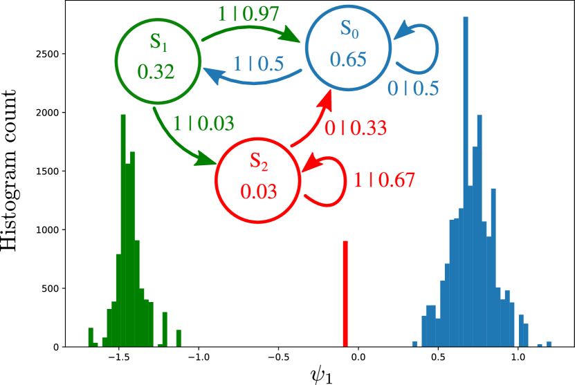
Figure 3: Even Process: Reconstructed-state coordinates $\psi_{1}$ on the first reduced-basis eigenvector $\Phi_{1}$, together with a graphical representation of the transitions inferred between the colored clusters.

The eigenvalue spectrum of the reduced basis decreases rapidly: $\lambda_{0}=1$ (as expected), $\lambda_{1}\approx 10^{-2}$, and all other eigenvalues $\lambda_{j\geq 2}<10^{-4}$. We therefore project the causal states on the only relevant eigenvector $\Phi_{1}$ and build the histogram shown in Fig. 3. Colors match labels automatically found by a clustering algorithm.

Figure 3 summarizes the cluster probabilities and their transitions. They match the original Even Process together with a transient causal state. By inspection, one sees this state represents the set of sequences of all $1$s mentioned above—the source of ambiguity. Its probability, for $L^{X}=10$, is that of jumping $5$ consecutive times from state $\sigma_{0}$ to state $\sigma_{1}$ in the generating Even Process. Hence, $1/2^{5}\approx 0.03$, which is the value we observe. From that transient state, the ambiguity cannot be resolved so transitions follow the $(1/3,2/3)$ proportions of the symbols in the series. Note that unifilarity is broken, since there are two paths for the symbol $v=1$ starting from state $\sigma_{1}$, also reflecting the ambiguity induced by the finite truncation.

VI.2 Infinite state complexity: An uncountable causal-state process

The Even Process is a case where ambiguity arises from incomplete knowledge, due to finite-range truncation. However, even for discrete finite data alphabets $\mathcal{V}$, there are process whose causal states are irreducibly infinite. This occurs generically for processes generated by nonunifilar HMMs. In this case, knowledge of the observed data is insufficient to determine the generative model’s internal state. Only distributions over those states—the mixed states [29]—are predictive.

In the limit $L^{X}\rightarrow\infty$, the causal states then correspond to unique mixed-state distributions [21] and there can be infinitely many (countable or uncountable) causal states, even for a simple finite generative HMMs. This arises from nonunifilarity since the same observed symbol allows transitions to two distinct internal states. In contrast, the predictive-equivalence determines that the same information (newly observed symbol), starting from the same current state (equivalence class $\epsilon(X)$ of pasts $X\in\mathcal{X}$), induces the same consequences (possible futures $Y$, with a fixed distribution $\Pr\left(Y|\epsilon(X)\right)$). Thus, nonunifilar models can be more compact generators. This can be beneficial, but it comes at the cost of being markedly-worse predictors than unifilar HMMs.

Consider the nonunifilar mess3 HMM introduced in Ref. 29, represented graphically in Fig. 4.

Figure 4: Nonunifilar generative HMM mess3: Only transition probabilities are depicted; emitted symbols are described in the main text.

Mess3 uses $3$ symbols $\mathcal{V}=\left\{0,1,2\right\}$ and consists of $3$ generative states $s_{0}$, $s_{1}$, and $s_{2}$. The state-transition diagram is symmetric and each state has the same transition structure. Consider the state $s_{i}$ for $i=0,1,2$ and modulo arithmetic so that $i-1=2$ when $i=0$ and $i+1=0$ when $i=2$. Then, the transitions are:

1. From state $s_{i}$ to itself, for a total probability $p=\alpha=ay+2bx$, symbols are emitted as $\Pr(v=i)=ay$ and $\Pr(v=i-1)=\Pr(v=i+1)=bx$.

2. From state $s_{i}$ to state $s_{i+1}$, for a total probability $p=(1-\alpha)/2$, symbols are emitted as $\Pr(v=i)=ax$, $\Pr(v=i-1)=bx$, and $\Pr(v=i+1)=by$.

3. From state $s_{i}$ to state $s_{i-1}$, for a total probability $p=(1-\alpha)/2$, symbols are emitted as $\Pr(v=i)=ax$, $\Pr(v=i-1)=by$, and $\Pr(v=i+1)=bx$.

In this, $a=0.6$, $b=(1-a)/2=0.2$, $x=0.15$, $y=1-2x=0.7$.

The generated process is known to give uncountably-infinite causal states. Their ensemble $\bm{\mathcal{S}}$ forms a Sierpinski gasket in the mixed-state simplex [29]. The probability to observe states at subdivisions decreases exponentially, though. With limited samples, only a few self-similar subdivisions of the main gasket triangle can be observed.

Reconstructing $\bm{\mathcal{S}}$ is performed using $L^{X}=15$ and $L^{Y}=1$. The same product exponential kernel is used as above, with a decay $\gamma=0.01$ and a bandwidth $\xi=0.1$. $N=25,000$ sample $\left(x,y\right)$ pairs are sufficient to reconstruct the first self-similar subdivisions.

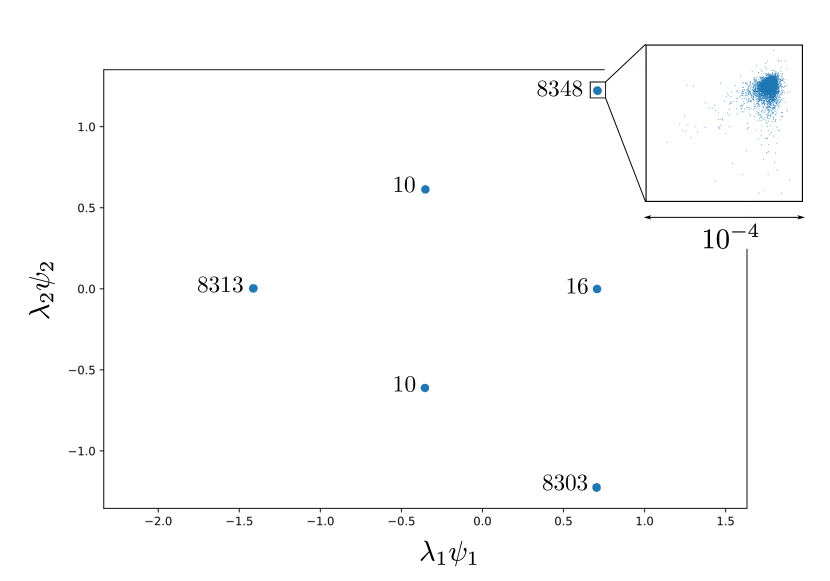
Figure 5: Projection of the mess3’s causal states on the reduced basis $\left\{\Phi_{1},\Phi_{2}\right\}$. The number of samples stacked on each point is indicated.

The eigenvalue spectrum is $\lambda_{0}=1$, $\lambda_{1}=0.999$, $\lambda_{2}=0.999$ and $\lambda_{i\geq 3}<1.2\times 10^{-15}$. The algorithm thus finds only two components, of equal significance. Figure 5 shows a scatter plot of the inferred causal states using coordinates in the reduced basis $\left\{\Phi_{1},\Phi_{2}\right\}$. The states are very well clustered on the main vertices of the Sierpinski Gasket. (The inset shows that $4$ orders of magnitude are needed to see a spread within each cluster, compared to the main triangle size.) The triangle is remarkably equilateral and its center even lies on $\approx(0,0)$, reflecting the symmetry of the original HMM. To our knowledge, no other algorithm is currently able to correctly recover the causal states purely from data from such a challenging, complex process.

The number of samples at each triangle node is indicated. The nodes at the first subdivision are about $800$ times less populated than the main nodes. While theory predicts that states appear on all subdivisions of the Sierpinski Gasket, the sample size needed to observe enough such states is out of reach computationally.

Figure 6: Lorenz attractor (left) and its estimated kernel $\epsilon$-machine (right) at various thermal $\eta$ and measurement $\nu$ noise levels.

VI.3 Thermally-driven Continuous Processes: Chaotic Lorenz attractors

The first two examples demonstrated that kernel $\epsilon$-machine reconstruction works well on discrete-valued data, even when states are expected to appear on a complicated fractal structure or when the time series has infinite-range correlations. The next step, and a central point of the development, is to reconstruct a continuous infinity of causal states from sampled data. The following example processes also serve to demonstrate time-series prediction using the estimated kernel $\epsilon$-machine, recalling the method introduced in Sec. IV.2.

We first use the chaotic Lorenz ordinary differential equations from 1963 with the usual parameters $\left(\sigma,\rho,\beta\right)=\left(10,28,8/3\right)$. [60] We add isotropic stochastic noise components $dW$ at amplitude $\eta$ to model thermal fluctuations driving the three main macroscopic fluid modes the ODEs were crafted to capture:

$$du =-\sigma\left(u-v\right)dt+\eta dW$$

$$dv =\left(\rho u-v-uw\right)dt+\eta dW$$

$$dw =\left(-\beta w+uv\right)dt+\eta dW\leavevmode\nobreak\ .$$

A random initial condition $\left(u_{0},v_{0},w_{0}\right)$ is drawn in the region near the attractor and a sufficiently long transient is discarded before collecting data $\left(u_{t},v_{t},w_{t}\right)$. SDE integration is performed using $dt=0.01$, yielding samples $\left(u_{t},v_{t},w_{t}\right)_{0\leq t<T}$ up to a maximal time $T$ corresponding to $N=20,000$ (past, future) pairs.

In addition to the thermal fluctuations, we also model systematic measurement error by adding a centered Gaussian process $\Gamma=\left(\gamma^{0},\gamma^{1},\gamma^{2}\right)$ with isotropic variance $\nu^{2}$. The result is the observed series $\left(u^{\prime}_{t},v^{\prime}_{t},w^{\prime}_{t}\right)=\left(u_{t}+\gamma_{t}^{0},v_{t}+\gamma_{t}^{1},w_{t}+\gamma_{t}^{2}\right)$ used to estimate a kernel $\epsilon$-machine and perform a sensitivity analysis.

VI.3.1 Kernel $\epsilon$-Machine reconstruction in the presence of noise and error

When $\eta=0$ and $\nu=0$ the deterministic ODEs’ trajectories do not cross and are uniquely determined by the initial condition $\left(u_{t},v_{t},w_{t}\right)$ at $t=0$. Hence, each state on the attractor is its own causal state. Retaining information from the past is moot, but only if $(u,v,w)$ is known with infinite precision, due to the ODEs’ chaotic solutions, that amplify fluctuations exponentially fast. This is never the case in practice. So, considering small values of $L^{X}$ and $L^{Y}$ may still be useful to better determine the causal states. We use $L^{X}=L^{Y}=5$ in the reconstructions.

Figure 6 shows the projections (right) with coordinates $\left(\psi_{1},\psi_{2},\psi_{3}\right)$, together with the original (pre-reconstruction) attractor data (left) for different noise combinations. Figure 6(top row) displays the results of kernel $\epsilon$-machine estimation from the noiseless data ($\nu=0$ and $\eta=0$). The second row shows the effects of pure measurement noise ($\nu=1$ and $\eta=0$) on the raw data (left) and on the estimated kernel $\epsilon$-machine (right). Similarly, the last row shows the effect of pure thermal noise ($\nu=0$ and $\eta=1$ .)

As expected, the structure is well recovered when no noise is added. A slight distortion is observed. In practice, the causal states are unaffected by coordinate transforms and reparametrizations of $X$ and $Y$ which do not change equivalence in conditional distributions $P\left(Y|X=x_{1}\right)\equiv P\left(Y|X=x_{2}\right)$, so the algorithm could very well have found another parametrization of the Lorenz-63 attractor. See also Section VI.4. The causal states of the original data series are also well recovered even when that series is severely corrupted by strong measurement noise at $\nu=1$ in Fig. 6(middle row).

To appreciate these results recall that, in the noiseless case, if $x_{1}$ and $x_{2}$ are in the same causal state $x_{2}\in\epsilon\left(x_{1}\right)$ of the original series, then by definition $\Pr\left(Y|X=x_{1}\right)=\Pr\left(Y|X=x_{2}\right)$. Measurement noise ($\nu>0$), independent at each time step, does not change this. Since measurement noise is added to each and every time step independently, noisy series $x^{\prime}$ ending with the same noisy triplet $\left(u^{\prime},v^{\prime},w^{\prime}\right)$ at the current time $t=t_{0}$ end up in the same causal state of the noisy system. This is reduced to the current triplet $\left(u^{\prime},v^{\prime},w^{\prime}\right)$, itself a specific causal state of the deterministic system. Hence, the causal states of the deterministic ODEs are subsets of those of kernel $\epsilon$-machine estimated from the noisy-measured series. We arrive at the important conclusion that, at least for deterministic chaotic systems, the uniqueness and continuity of ODE solutions guarantee that causal states are unaffected by measurement noise. This is generally not true for many-to-one maps and other functional state-space transforms that merge states.

In contrast to measurement noise, thermal noise ($\eta>0$) modifies the equations of motion and the resulting trajectories reflect the accumulated perturbations. Since each state on the (deterministic) attractor is its own state, the estimated causal states are modified.

Let’s probe the robustness of kernel $\epsilon$-machine estimation. With the parameters detailed below, we obtain an eigenvalue spectrum shown in Fig. 7. There is an inflection point after the first three components. The eigenvalues are remarkably insensitive to a strong measurement noise level $\nu=1$. They are also very robust to the thermal noise $\eta=1$, which induces only some minor eigenvalue changes.

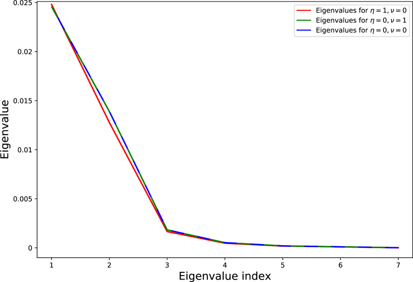
Figure 7: Eigenvalues for the Lorenz-63 attractor estimated kernel $\epsilon$-machines at various thermal and measurement noise levels.

Thus, kernel $\epsilon$-machine estimation achieves a form of denoising beneficial for random dynamical systems. However, the reconstructed causal states reflect the thermal noise induced by $\eta=1$, as can be seen in the fine details of the bottom row of Fig. 6. Note that the algorithm is able to strongly reduce the measurement noise, and do so even while the attractor is very corrupted, while the apparently minor thermal noise is preserved.

VI.3.2 Kernel $\epsilon$-Machine prediction and sensitivity

In Ref. 46, a prediction experiment is performed using an evolution operator computed directly in $\left(u,v,w\right)$ space instead of in $\bm{\mathcal{S}}$, as here; recall Sec. V.3. That study focuses on how the error due to a small perturbation propagates with the number of prediction steps.

Here, we use a more typical approach to first learn the model—i.e., compute the states, the basis $\Phi$, the evolution operator, …—on a data set of $N=20,000$ samples. Then, however, we estimate the prediction error on a completely separate “test” set. This data set is generated with the same parameters as for the training set, but starting from another randomly drawn initial condition. $P=100$ test samples are selected after the transient, each separated by a large subsampling interval so as to reduce their correlation. Unlike the examples in the previous sections, this produces an objective error function—the prediction accuracy—useful for cross-validating the relevant meta-parameters.

Due to the computational cost involved with grid searches, we only cross-validate the data kernel $k^{V}$ bandwidth on a reduced data set in preliminary experiments. In Ref. 46, an arbitrary variance was chosen for the distribution used to project $\left(u,v,w\right)$ triplets onto the operator eigenbasis. We also cross-validate it to improve the results, for a fair comparison with kernel $\epsilon$-machine reconstruction.

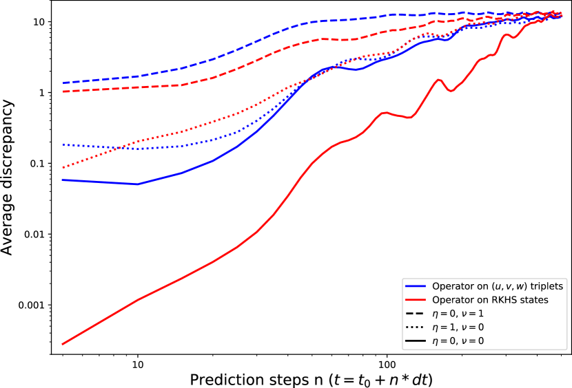
Figure 8: Predictions on the Lorenz-63 attractor.

Figure 8 presents the results. Forecasts are produced at every $\Delta t=0.05$ interval and operator exponentiation is used in between, as detailed in Sec. V.3. This allows a comparison of trajectories over $500$ elementary integration steps, which is large enough for the trajectory to switch between the attractor main lobes several times. Such trajectories are computed starting from each of the $100$ test samples.

In the noiseless case $\eta=\nu=0$, the average discrepancy $\left\langle\left\|\left(u,v,w\right)-\left(u_{p},v_{p},w_{p}\right)\right\|\right\rangle$ measures how predicted triplets $\left(u_{p},v_{p},w_{p}\right)$ differ from data triplets $\left(u,v,w\right)$, averaged at each prediction step over the $100$ trajectories.

In the noisy cases, it make little sense to test the algorithm’s ability to reproduce noisy data. We instead test its ability to predict accurately the noiseless series $\left(u,v,w\right)_{t>t_{0}}$ based on noisy past observations $\left(u^{\prime},v^{\prime},w^{\prime}\right)_{t\leq t_{0}}$. This is easily done for measurement noise $\nu>0$, for which the original noiseless series is available by construction.

For simulated thermal noise $\eta>0$, all we have is a particular realization of an SDE, but no clean reference. Starting from the current noisy values at each prediction point $\left(u^{\prime},v^{\prime},w^{\prime}\right)$, we evolve a noiseless trajectory with the basic Lorenz ODE equations. Since we use an isotropic centered $\eta dW$ Wiener process, that trajectory is also the ensemble average over many realizations of the SDE, starting from that same $\left(u^{\prime},v^{\prime},w^{\prime}\right)$ point. It makes more sense to predict that ensemble average, from the current noisy causal-state estimate, rather than a particular SDE trajectory realization.

The results in Fig. 8 show a clear gain in precision when using the RKHS method, both in the unperturbed data case and when data is perturbed by measurement noise $\nu=1$. This gain persists until the trajectory becomes completely uncorrelated with the original prediction point. The situation is less favorable for thermal noise $\eta=1$.

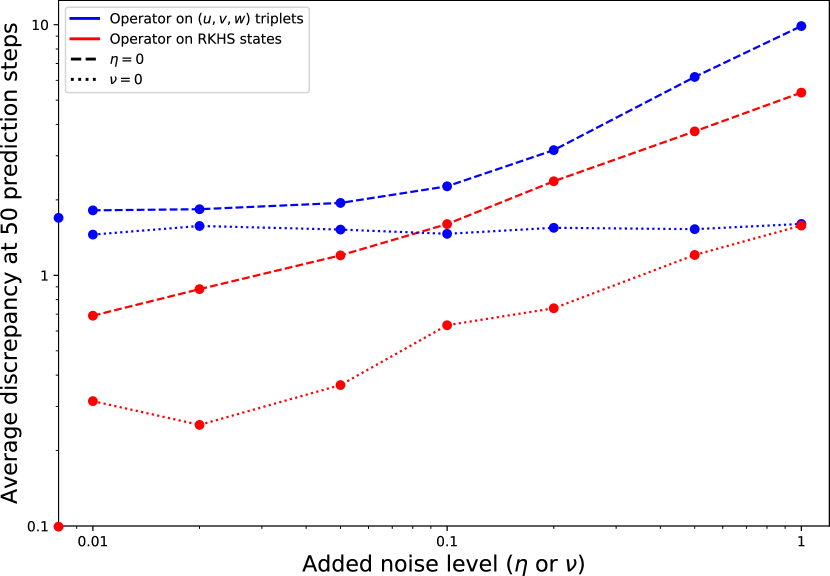
Figure 9: Sensitivity when predicting trajectories along the Lorenz-63 attractor: Reconstruction error dependency on noise levels. Data for the $\nu=\eta=0$ noiseless case is shown as markers on the vertical axis.

Figure 9 presents a sensitivity analysis that focuses on predictions after $50$ time steps. For lower noise levels $\eta<1$, the RKHS method still improves the prediction error, while the operator in data space does not seem to be sensitive to $\eta$. We note (not shown here) that, for longer time scales, the RKHS method may produce worse results on average. The handling of measurement noise $\nu<1$ is also in favor of the RKHS method, consistent with above results.

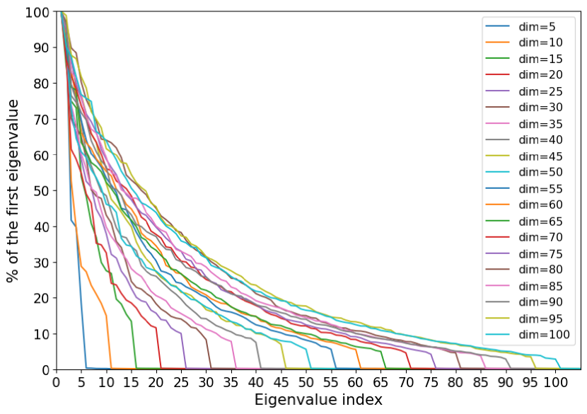
Figure 10: Eigenvalues for the reconstruction of Lorenz-96 attractor, randomly projected in dimension 1000, with added high-dimensional noise, for $N=10000$ samples. The dimension in the legend refers to the original parametrization of Lorenz-96 attractor, which is recovered by the algorithm in the form of a spectral gap when reconstructed from the 1000-dimensional noisy time series. Values after the gap are very low and given in Table 1, together with the gap itself.

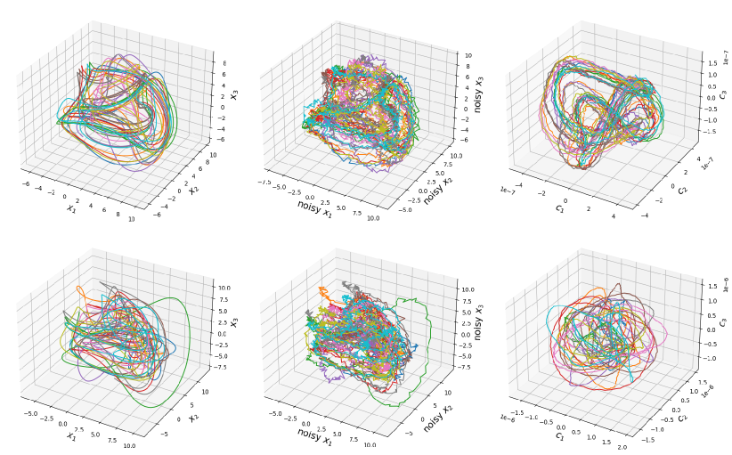
Figure 11: (Top left) First 3 components of the Lorenz-96 $D=5$-dimensional attractor, with $N=5000$ samples. (Top middle) Same, back projected into the original space from the noisy 1000-dimensional random embedding. (Top right) First 3 coordinates of the causal states set $\bm{\mathcal{S}}$ reconstruction. (Bottom row) same plots for the $D=100$-dimensional Lorenz-96 formulation. The reconstructed coordinates can be equivalent reparametrizations of the original variables and need not match those $1$ to $1$. In each case the noise has been greatly reduced, as in Fig. 6. Colors correspond to $10$ time series, each starting from a distinct random location on the basin of attraction, taken after a sufficiently long transient.

Dim. $D$	$5$	$10$	$15$	$20$	$25$	$30$	$35$	$40$	$45$	$50$	$55$	$60$	$65$	$70$	$75$	$80$	$85$	$90$	$95$	$100$
$100\frac{\lambda_{D+1}}{\lambda_{1}}$	0.31	0.23	0.26	0.24	0.24	0.24	0.22	0.25	0.26	0.21	0.23	0.23	0.23	0.22	0.23	0.26	0.24	0.20	0.25	0.21
$\frac{\lambda_{D}}{\lambda_{D+1}}$	60.3	64.1	51.2	49.3	42.2	35.2	34.9	30.8	26.8	26.4	25.1	24.1	22.0	20.7	18.5	18.1	15.8	14.3	14.5	13.9

Table 1: Top row: Dimension of the Lorenz-96 ODE system; that is, before trajectories on the attractor undergo random projection and adding noise. Middle row: Eigenvalue after the spectral gap, expressed in % of the first eigenvalue. Bottom row: Spectral gaps, relative to the value after the gap. Results for $N=10000$ samples are graphically presented in Fig. 10.

	$N=5000$			$N=10000$			$N=20000$
Dim. $D$	$90$	$95$	$100$	$90$	$95$	$100$	$90$	$95$	$100$
$100\frac{\lambda_{D+1}}{\lambda_{1}}$	$0.22$	$0.18$	$0.21$	$0.20$	$0.25$	$0.21$	$0.21$	$0.20$	$0.21$
$\frac{\lambda_{D}}{\lambda_{D+1}}$	$6.3$	$5.8$	$5.0$	$14.3$	$14.5$	$13.9$	$26.1$	$25.6$	$26.5$

Table 2: Spectral gap dependency on the number $N$ of samples: Eigenvalues after the gap do not change in magnitude. Spectral gaps themselves, though, are much better resolved for larger $N$, especially in higher dimensions $D$.

VI.4 Behavior with high-dimensional data and attractors

This is all well and good, but do attractor reconstruction and denoising capabilities hold in higher dimensions? In fact, it has been known for decades [61] that the Lorenz-63 system is special and very easily reconstructed. This is due to its high state-space volume contraction rate and its simple and smooth vectorfield that sports only two nonlinear terms.

To address these issues, we employ the Lorenz 1996 model, [62] with tuneable dimension parameter $D$, defined for $i=1\ldots D$ by $du_{i}/dt=-u_{i-2}u_{i-1}+u_{i-1}u_{i+1}-u_{i}+F$, with modulo arithmetic on the indices. We use $F=8$, which yields chaotic dynamics. In order to better cover all of the attractor, series are generated from $10$ different starting points taken at random on the bassin of attraction, after discarding a sufficiently long transient. $N$ samples of $\left(x,y\right)$ pairs are collected from these series, using history lengths of $L^{X}=L^{Y}=5$ values of vectors $u$. The projection of these series along the first 3 dimensions of the attractors for $D=5$ and $D=100$ are shown on the left part of Fig. 11.

To test the algorithm’s reconstruction performance, we embed the time series in a $1000$-dimensional space using random projections: $V=UR$ with $R$ a matrix of random components of size $D\times 1000$, taken from a normal distribution of standard deviation $1/D$. $U$ holds the collected samples, organized in a matrix of size $N\times D$. In practice, in such high dimension, the projection directions in $R$ are nearly orthogonal. In addition, Gaussian noise with variance $\nu^{2}=1/D$ is added to each component of $V$, similar to the setup in Section VI.3.1. We use the resulting data $W=V+\textrm{noise}$ as input to the algorithm: Truly 1000-dimensional data, now leaking into all dimensions thanks to the added noise, while retaining the overall lower $D$-dimensional structure of the Lorenz-96 attractor. This experiment seeks to reconstruct this hidden $D$-dimensional structure, solely from noisy $1000$-dimensional time series.

The middle panes of Fig. 11 show the corrupted $W$ data, projected back into the original space using the pseudo-inverse $pinv\left(R\right)$, for $D=5$ and $D=100$. The scaling of the noise variance makes it so the strength of the noise is similar irrespective of $D$.

The right panel of Fig. 11 shows the well-reconstructed attractor. Moreover, the denoising for chaotic attractors observed in Section VI.3.1 is also well reproduced in this markedly more complicated setting. Interestingly, the first 3 coordinates of the reconstructed attractor do not, and need not, match that of the original $U$ series. Indeed, the causal states are equivalence classes of conditional distributions and, as such, are invariant by reparametrizations of the original data that preserve these equivalence classes; such as, coordinate transformations.

We see that the algorithm finds a parametrization where each added coordinate best encodes the conditional distributions in the low-dimensional coordinate representation, as explained in Section IV.3. Yet, that parametrization encodes each and every initial $D$ component, even though it is presented with $1000$-dimensional noisy time series of lengths $L^{X}=L^{Y}=5$. This is shown in Fig. 10 and Table 1, which clearly demonstrate spectral gaps at exactly $D$ reconstructed components. These spectral gaps are more pronounced as the number of samples $N$ increases, as shown in Table 2. As expected, a larger number of samples $N$ is required for properly capturing the spectral gaps as the dimension $D$ increases.

VII Conclusion

We introduced kernel $\epsilon$-machine reconstruction—a first-principles approach to empirically discovering causal structure. The main step was to represent computational mechanics’ causal states in reproducing kernel Hilbert spaces. This gave a mathematically-principled method for estimating optimal predictors of minimal size and so for discovering causal structure in data series of wide-ranging types.

Practically, it extends computational mechanics to nearly arbitrary data types. (At least, those for which a characteristic reproducing kernel exists.) Section III.1 showed, though, that this includes heterogeneous data types via kernel compositions.

Based on this, we presented theoretical arguments and analyzed cases for which causal-state trajectories are continuous. In this setting, the kernel $\epsilon$-machine is equivalent to an Itô diffusion acting on the structured set of causal states—a time-homogeneous, state-heterogeneous diffusion. The generator of that diffusion and its evolution operator can be estimated directly from data. This allows efficiently evolving causal-state distributions in a way similar to a Fokker-Plank equation. This, in turn, facilitates predicting a process in its original data space in a new way; one particularly suited to time series analysis.

Future efforts will address the introduction of discontinuities, which may arise for reasons mentioned in Sec. IV.1. This will be necessary to properly handle cases where data sampling has occurred above the scale at which time and causal-state trajectories can be considered continuous. Similarly, when the characteristic scale of the observed system dynamics is much larger than the sampling scale, a model reproducing the dynamics of the sampled data may simply not be relevant. Extensions of the current approach are thus needed, possibly incorporating jump components to properly account for a measured system’s dynamics at different scales. This, of course, will bring us back to the computational mechanics of renewal and semi-Markov processes.[5]

Another future challenge is to extend kernel $\epsilon$-machine reconstruction to spatiotemporal systems, where temporal evolution depends not only on past times but also on spatially-nearby state values.[27, 8, 63, 64] An archetypal example of these systems is found with cellular automata. In fact, any numerical finite elements simulation performed on discrete grids also falls into this category, including reaction-diffusion chemical oscillations and hydrodynamic flows. Spacetime complicates the definition of the evolution operator, compared to that of time series. However, the applicability of kernel $\epsilon$-machine reconstruction would be greatly expanded to a large category of empirical data sets.

Last, but not least, are the arenas of information thermodynamics and stochastic thermodynamics. In short, it is time to translate recent results on information engines and their nonequilibrium thermodynamics [21, 22, 23, 28] to this broadened use of computational mechanics. This, in addition to stimulating theoretical advances, has great potential for providing new and powerful tools for analyzing complex physical and biological systems, not only their dynamics and statistics, but also their energy use and dissipation.

Data and code availability

The source code for the method described in this document is provided as free/libre software and is available from this page: https://team.inria.fr/comcausa/continuous-causal-states/. Experiments in sections VI.1, VI.2 and VI.3 can be reproduced by retrieving the tagged version “first_arxiv” from the GIT archive, the experiment in Section VI.4 with the tagged version “chaos_submission”.

Reference

References

- [1] J. P. Crutchfield and K. Young. Inferring statistical complexity. Phys. Rev. Let., 63:105–108, 1989.
- [2] J. P. Crutchfield. Between order and chaos. Nature Physics, 8:17–24, 2012.
- [3] C. R. Shalizi and J. P. Crutchfield. Computational mechanics: Pattern and prediction, structure and simplicity. J. Stat. Phys., 104:817–879, 2001.
- [4] S. E. Marzen and J. P. Crutchfield. Inference, prediction, and entropy-rate estimation of continuous-time, discrete-event processes. arxiv:2005.03750.
- [5] S. Marzen and J. P. Crutchfield. Structure and randomness of continuous-time discrete-event processes. J. Stat. Physics, 169(2):303–315, 2017.
- [6] C. R. Shalizi, K. L. Shalizi, and J. P. Crutchfield. Pattern discovery in time series, Part I: Theory, algorithm, analysis, and convergence. 2002. arXiv.org/abs/cs.LG/0210025.
- [7] G. M. Goerg and C. R. Shalizi. Mixed LICORS: A nonparametric algorithm for predictive state reconstruction. Artificial Intelligence and Statistics, pages 289 – 297, 2013.
- [8] A. Rupe, N. Kumar, V. Epifanov, K. Kashinath, O. Pavlyk, F. Schlimbach, M. Patwary, S. Maidanov, V. Lee, Mr. Prabhat, et al. DisCo: Physics-based unsupervised discovery of coherent structures in spatiotemporal systems. In 2019 IEEE/ACM Workshop on Machine Learning in High Performance Computing Environments (MLHPC), pages 75–87. IEEE, 2019.
- [9] Nicolas Brodu. Quantifying the effect of learning on recurrent spikin neurons. In 2007 International Joint Conference on Neural Networks, pages 512–517. IEEE, 2007.
- [10] S. Klus, I. Schuster, and K. Muandet. Eigendecompositions of transfer operators in reproducing kernel hilbert spaces. J. Nonlin. Sci., 30(1):283–315, 2020.
- [11] C. C. Strelioff and J. P. Crutchfield. Bayesian structural inference for hidden processes. Phys. Rev. E, 89:042119, 2014.
- [12] S. Marzen and J. P. Crutchfield. Predictive rate-distortion for infinite-order markov processes. J. Stat. Phys., 163(6):1312–1338, 2014.
- [13] R. J. Elliot, L. Aggoun, and J. B. Moore. Hidden Markov Models: Estimation and Control, volume 29 of Applications of Mathematics. Springer, New York, 1995.
- [14] C. R. Shalizi and K. L. Klinkner. Blind construction of optimal nonlinear recursive predictors for discrete sequences. In M. Chickering and J. Y. Halpern, editors, Uncertainty in Artificial Intelligence: Proceedings of the Twentieth Conference (UAI 2004), pages 504–511, Arlington, Virginia, 2004. AUAI Press.
- [15] N. Brodu. Reconstruction of epsilon-machines in predictive frameworks and decisional states. Adv. Complex Syst., 14(05):761 – 794, 2011.
- [16] R. J. Elliott, L. Aggoun, and J. B. Moore. Hidden Markov models: Estimation and control. Springer, New York, 1994.
- [17] C. R. Shalizi, K. L. Shalizi, and R. Haslinger. Quantifying self-organization with optimal predictors. Phys. Rev. Lett., 93:118701, 2004.
- [18] A. Jurgens and J. P. Crutchfield. Shannon entropy rate of hidden Markov processes. J. Statistical Physics, 183(32):1–18, 2020.
- [19] A. Jurgens and J. P. Crutchfield. Divergent predictive states: The statistical complexity dimension of stationary, ergodic hidden Markov processes. Chaos, 31(8):0050460, 2021.
- [20] A. Jurgens and J. P. Crutchfield. Minimal embedding dimension of minimally infinite hidden Markov processes. in preparation, 2020.
- [21] C. J. Ellison, J. R. Mahoney, and J. P. Crutchfield. Prediction, retrodiction, and the amount of information stored in the present. J. Stat. Phys., 136(6):1005–1034, 2009.
- [22] J. P. Crutchfield, C. J. Ellison, and J. R. Mahoney. Time’s barbed arrow: Irreversibility, crypticity, and stored information. Phys. Rev. Lett., 103(9):094101, 2009.
- [23] P. M. Riechers and J. P. Crutchfield. Spectral simplicity of apparent complexity. II. exact complexities and complexity spectra. Chaos, 28(033116), 2018.
- [24] J. E. Hanson and J. P. Crutchfield. Computational mechanics of cellular automata: An example. Physica D, 103:169–189, 1997.
- [25] C. S. McTague and J. P. Crutchfield. Automated pattern discovery—an algorithm for constructing optimally synchronizing multi-regular language filters. Theoretical Computer Science, 359(1-3):306–328, 2006.
- [26] C. R. Shalizi, R. Haslinger, J.-B. Rouquier, K. L. Klinkner, and C. Moore. Automatic filters for the detection of coherent structure in spatiotemporal systems. Phys. Rev. E, 73(3):036104, 2006.
- [27] A. Rupe and J. P. Crutchfield. Local causal states and discrete coherent structures. Chaos, 28(7):1–22, 2018.
- [28] P. M. Riechers and J. P. Crutchfield. Fraudulent white noise: Flat power spectra belie arbitrarily complex processes. Physical Review Research, 3(1):013170, 2021. arXiv:1908.11405.
- [29] S. E. Marzen and J. P. Crutchfield. Nearly maximally predictive features and their dimensions. Phys. Rev. E, 95(5):051301(R), 2017.
- [30] S. Marzen and J. P. Crutchfield. Informational and causal architecture of continuous-time renewal processes. J. Stat. Phys., 168(a):109–127, 2017.
- [31] S. Marzen, M. R. DeWeese, and J. P. Crutchfield. Time resolution dependence of information measures for spiking neurons: Scaling and universality. Front. Comput. Neurosci., 9:109, 2015.
- [32] A. Smola, A. Gretton, Le Song, and B. Schölkopf. A Hilbert Space Embedding for Distributions. In Algorithmic Learning Theory: 18th International Conference, volume 31, pages 13 – 31, 2007.
- [33] L. Song, J. Huang, A. Smola, and K. Fukumizu. Hilbert space embeddings of conditional distributions with applications to dynamical systems. In Proceedings of the 26th Annual International Conference on Machine Learning, pages 961 – 968. ACM, 2009.
- [34] N. Aronszajn. Theory of Reproducing Kernels. Trans. Amer. Math. Soc., 68(3):337 – 404, 1950.
- [35] B. E. Boser, I. M. Guyon, and V. N. Vapnik. A training algorithm for optimal margin classifiers. In Proc. Fifth Annual Workshop on Computational Learning Theory, pages 144–152, 1992.
- [36] A. Gretton, K. M. Borgwardt, M. J. Rasch, B. Schölkopf, and A. Smola. A kernel two-sample test. J. Mach. Learn. Res., 13:723 – 773, 2012.
- [37] B. Sriperumbudur, A. Gretton, K. Fukumizu, B. Schoelkopf, and G. Lanckriet. Hilbert Space Embeddings and Metrics on Probability Measures. J. Mach. Learn. Res., 11:1517 – 1561, 2010.
- [38] L. Song, K. Fukumizu, and A. Gretton. Kernel embeddings of conditional distributions: A unified kernel framework for nonparametric inference in graphical models. IEEE Signal Processing Magazine, 30(4):98 – 111, 2013.
- [39] K. Fukumizu, L. Song, and A. Gretton. Kernel Bayes’ rule: Bayesian inference with positive definite kernels. The Journal of Machine Learning Research, 14(1):3753 – 3783, 2013.
- [40] S. Grünewälder, G. Lever, L. Baldassarre, S. Patterson, A. Gretton, and M. Pontil. Conditional mean embeddings as regressors. In Proceedings of the 29th International Conference on Machine Learning, 2012.
- [41] B. Schölkopf, R. Herbrich, and A. J. Smola. A generalized representer theorem. In International conference on computational learning theory, pages 416 – 426. Springer, 2001.
- [42] P. Honeine and C. Richard. Solving the pre-image problem in kernel machines: A direct method. In 2009 IEEE Intl. Workshop on Machine Learning for Signal Processing, pages 1–6. IEEE, 2009.
- [43] I. Schuster, M.attes Mollenhauer, S. Klus, and K. Muandet. Kernel conditional density operators. In Intl. Conf. on Artificial Intelligence and Statistics, pages 993–1004. PMLR, 2020.
- [44] For Itô diffusions, these are compactly-supported and twice differentiable.
- [45] K. Jacobs. Stochastic processes for physicists: Understanding noisy systems. Cambridge University Press, 2010.
- [46] T. Berry, D. Giannakis, and J. Harlim. Nonparametric forecasting of low-dimensional dynamical systems. Phys. Rev. E, 91(3):032915, 2015.
- [47] It may be that ’s dimension is actually infinite, so that its estimate grows with the number of samples. This can be detected using the spectral method presented in the main text.
- [48] R. R. Coifman and S. Lafon. Diffusion maps. Appl. Comput. Harmon. Anal., 21(1):5 – 30, 2006.
- [49] T. Berry and J. Harlim. Variable bandwidth diffusion kernels. Applied and Computational Harmonic Analysis, 40(1):68–96, 2016.
- [50] T. Berry and T. Sauer. Local kernels and the geometric structure of data. Applied and Computational Harmonic Analysis, 40(3):439–469, 2016.
- [51] R. R. Coifman, S. Lafon, A. B. Lee, M. Maggioni, B. Nadler, F. Warner, and S. W. Zucker. Geometric diffusions as a tool for harmonic analysis and structure definition of data: Diffusion maps. Proc. Natl. Acad. Sci. USA, 102(21):7426–7431, 2005.
- [52] R. R. Coifman, Y. Shkolnisky, F. J. Sigworth, and A. Singer. Graph Laplacian tomography from unknown random projections. IEEE Trans. Image Proc., 17(10):1891–1899, 2008.
- [53] R. R. Coifman, S. Lafon, A. B. Lee, M. Maggioni, B. Nadler, F. Warner, and S. W. Zucker. Geometric diffusions as a tool for harmonic analysis and structure definition of data: Multiscale methods. Proc. Natl. Acad. Sci. USA, 102(21):7432–7437, 2005.
- [54] P. Drineas and M. W. Mahoney. On the Nyström method for approximating a gram matrix for improved kernel-based learning. J. Machine Learning Research, 6(Dec):2153–2175, 2005.
- [55] L. Song, X. Zhang, A. Smola, A. Gretton, and B. Schölkopf. Tailoring density estimation via reproducing kernel moment matching. In Proc. 25th Intl. Conf. Machine learning, pages 992–999, 2008.
- [56] R. Friedrich, J. Peinke, M. Sahimi, and M. R. R. Tabar. Approaching complexity by stochastic methods: From biological systems to turbulence. Physics Reports, 506(5):87–162, 2011.
- [57] R. Alexander and D. Giannakis. Operator-theoretic framework for forecasting nonlinear time series with kernel analog techniques. Physica D: Nonlinear Phenomena, page 132520, 2020.
- [58] Here DBSCAN with threshold 0.1 was used. However, any reasonable clustering algorithm will work given that clusters are well separated.
- [59] The probabilities sum exactly to . We show all the transitions found.
- [60] E. N. Lorenz. Deterministic nonperiodic flow. J. Atmos. Sci., 20:130, 1963.
- [61] J. P. Crutchfield and B. S. McNamara. Equations of motion from a data series. Complex Systems, 1:417 – 452, 1987.
- [62] Edward N Lorenz. Predictability: A problem partly solved. In Proc. Seminar on Predictability, volume 1, 1996.
- [63] A. Rupe, K. Kashinath, N. Kumar, V. Lee, Prabhat, and J. P. Crutchfield. Towards unsupervised segmentation of extreme weather events. arxiv:1909.07520.
- [64] A. Rupe and J. P. Crutchfield. Spacetime autoencoders using local causal states. AAAI Fall Series 2020 Symposium on Physics-guided AI for Accelerating Scientific Discovery, 2020. arXiv:2010.05451.