Applying Convolutional Neural Networks to Data on Unstructured Meshes with Space-Filling Curves
Abstract
This paper presents the first classical Convolutional Neural Network (CNN) that can be applied directly to data from unstructured finite element meshes or control volume grids. CNNs have been hugely influential in the areas of image classification and image compression, both of which typically deal with data on structured grids. Unstructured meshes are frequently used to solve partial differential equations and are particularly suitable for problems that require the mesh to conform to complex geometries or for problems that require variable mesh resolution. Central to our approach are space-filling curves, which traverse the nodes or cells of a mesh tracing out a path that is as short as possible (in terms of numbers of edges) and that visits each node or cell exactly once. The space-filling curves (SFCs) are used to find an ordering of the nodes or cells that can transform multi-dimensional solutions on unstructured meshes into a one-dimensional (1D) representation, to which 1D convolutional layers can then be applied. Although developed in two dimensions, the approach is applicable to higher dimensional problems.
To demonstrate the approach, the network we choose is a convolutional autoencoder (CAE), although other types of CNN could be used. The approach is tested by applying CAEs to data sets that have been reordered with a space-filling curve. Sparse layers are used at the input and output of the autoencoder, and the use of multiple SFCs is explored. We compare the accuracy of the SFC-based CAE with that of a classical CAE applied to two idealised problems on structured meshes, and then apply the approach to solutions of flow past a cylinder obtained using the finite-element method and an unstructured mesh.
keywords:
Convolutional Neural Network , Space-Filling Curve , Unstructured Meshes , Autoencoder , Convnets1 Introduction
Also known as convnets, Convolutional Neural Networks (CNNs) have provided revolutionary advances in the fields of image compression [1, 2] and image classification [3, 4]. Although most often encountered in computer vision, technology from CNNs has recently shown promise in helping to solve governing equations for fluid motion [5], as well as analysing these motions [6]. The accuracy of CNNs for image compression seems to carry over to these applications, however, CNN technology is generally based on structured grids and is, therefore, not readily applicable to data held on unstructured meshes. Many computational fluid dynamics (CFD) problems rely on unstructured meshes to resolve complex geometries [7] and interfaces [8]. These meshes typically have more resolution where needed, that is, where finer-scale features occur, such as in the vicinity of a viscous boundary layer, at the interface between fluids, at a density front or shock wave [9, 10].
Without a means of applying CNN techniques directly to data on unstructured meshes, a number of other methods have been developed. One may apply a 1D CNN directly to the vectorised nodal values of the solution variables. If the ordering of these variables has been optimised, to increase the efficiency of iterative or direct solvers for example, this might be more successful, however, we have found that this approach either does not work or has limited success. To improve this method, one could interpolate the data from an unstructured mesh to a structured mesh and then apply a CNN, although this will introduce errors due to interpolation and generally requires a much larger number of grid points to capture the features in the original data [11]. Of course, one could also restrict oneself to using structured meshes for the solution data and then apply CNNs directly to this [5, 12, 13]. However, for modelling certain geometries or physics, this is not feasible.
Graph-based methods can also be used to apply CNNs to arbitrary data that has been arranged in the form of a graph. Graph Neural Networks (GNNs) are networks that can be applied to such data [14], for example, the data associated with an unstructured finite element mesh that has been transformed to a graph. As in classical CNNs, convolutional GNNs [14] or Graph Convolutional Networks [15] take a weighted average of the values at the vertices (or pixels or cells) adjacent to a given vertex and use this to form a new layer or feature map similar to classical CNNs. Recently developed within PyTorch [16], MeshCNN [17] is one example of this type of method. MeshCNN forms a graph from the discretisation and then applies convolutional filters directly to the data held on the unstructured mesh by using mesh coarsening operations, akin to those used in multi-grid methods [18]. The resulting coarse meshes are then used to form pooling operations similar to those used in classical CNNs. MeshCNN [17] has a higher accuracy than other methods when tested on a variety of classification and segmentation problems. Another type of graph-based methods are Point Cloud methods [19], which form a graph from the nearest neighbouring points to a given point in the data cloud. Once the graph is constructed, convolutional filters can be applied as described above. Such point cloud methods may be very useful for working with data represented on a series of different meshes, for example, arising from the use of mesh adaptivity [20], as there may be no need to re-train the neural network. Graph networks (a type of GNN), which learn interactions between variables in a compressed space, have successfully been applied to problems in fluid and solid dynamics [21, 22]. Both approaches use an encoder and decoder to compress and reconstruct the data, and a time-stepping method for predicting the future solution variables. The former uses particle-based methods to solve the governing equations, and exploits a nearest-neighbour technique to form an underlying graph of interactions. The latter applies the finite-element method to solve the governing equations and simply uses the underlying finite-element discretisation as the graph, combined with a neighbourhood graph for modelling solid-cloth dynamics. In both cases, the graph is used to learn the dynamics of the systems.
By using Space-Filling Curves (SFCs), we demonstrate in this paper that one can apply the traditional CNN approaches (in 1D) directly to data held on unstructured multi-dimensional meshes. The underlying ideas of space-filling curves are applied to produce a continuous curve through a finite element mesh, in which the curve traverses every node of the mesh. This space-filling curve is used to transform multi-dimensional data into 1D data, to which convolutional layers are then applied. Sparse layers are introduced to the network, which add some smoothing to the results. The use of multiple SFCs is also explored in this paper.
The first eponymous space-filling curve was discovered by Peano in 1890 [23], when seeking a continuous mapping from the unit interval onto the unit square. One year later, Hilbert introduced a variant of this curve [24] known as a Hilbert curve or Hilbert space-filling curve. Since then, many other SFCs have been developed including those by Moore, Lebesgue, Sierpiński [25, 26]. Ideal for transforming and reordering multi-dimensional data to 1D data, space-filling curves:
-
(P1)
generate a continuous curve in which neighbours of any node within that curve are nodes that are close to one another;
-
(P2)
have in-built hierarchies of features, for example, if one takes every points along the curve, the result is a coarser mesh across the whole domain;
-
(P3)
are Lebesgue-measure preserving (at least the classical SFCs have this property), so that sub-curves of equal length fill multi-dimensional regions of equal area or volume.
The properties of space-filling curves have already been exploited in a number of techniques used in the numerical solution of partial differential equations. For example, property P1 has led to the use of SFC orderings to manage cache memory when calculating matrix-matrix or matrix-vector products [27]. Properties P1 and P2 have led to the use of SFCs to optimise the node numbering for the benefit of iterative solvers [28]. Properties P2 and P3 have resulted in the extensive use of SFCs with unstructured meshes to find a partition suitable for parallel computing [29]. That is, if one slices the SFC into equal intervals, then the result is a domain decomposition that has partitions with minimal connectivity (few common edges) between the partitions.
Space-filling curves are a natural partner to CNNs because of properties P1, P2 and P3, and have been applied to structured grids to reduce 3D structured grid data to 1D in image compression [30, 31]. They have also been applied to DNA sequencing and classification [32, 33]. The latter compares different mappings of 2D structured mesh data to 1D, to which a CNN is applied, and found that the mappings based on Hilbert SFCs performed the best. Analysis of SFCs for their data preserving abilities is investigated in [34]. Applying 1D CNNs to 2D data that has been transformed by an SFC has also displayed comparable accuracy and speed to classical 2D and 3D CNNs [35], again, for data on structured grids.
We present here a method of applying CNNs directly to data on unstructured meshes, such as solutions arising from finite element or control volume discretisations. The method is timely as researchers are currently looking to improve compression or dimensionality reduction methods within reduced-order model frameworks [5, 11, 12, 13, 36] by exploiting some of the useful properties of CNNs, such as the multiscale resolution, rotational and position invariance [37, 3, 5]. Reduced-order models often rely on Singular Value Decomposition (SVD) for compression (or dimension reduction) through Proper Orthogonal Decomposition (POD) [38, 39, 40, 41]. SVD-based methods can be limited in their abilities to interpolate solutions, for example, suffering from Gibbs oscillations when there are abruptly changing fields [12] and poor accuracy for convection-dominated problems [41]. Going some way to tackle this, a combination of SVD and a fully-connected autoencoder is presented as a tool for dimension reduction in [36], however, some of the issues of the SVD are still present. Thus, being able to apply CNNs to data on unstructured meshes could significantly improve the quality of such reduced-order models. In addition to the timely nature of this work, the elegant SFC-based approach outlined here, is expected to be computationally faster than the graph-based approaches (MeshCNN and GNNs), since the latter will be dominated by indirect addressing. In the method outlined here, there is only indirect addressing at the inputs and outputs of the space-filling curve CNN and then, only when multiple space-filling curves are used.
The remainder of this paper is as follows. The following section describes how space-filling curves are formed for an unstructured mesh. The architectures of the convolutional autoencoders used in this paper are described in Section 3. The results are presented in Section 4 which includes the application of SFC-based autoencoders to data on a structured mesh (for advection of a square wave and advection of a Gaussian function) and data on an unstructured mesh (for flow past a cylinder). Future work is then discussed and conclusions are drawn.
2 Determining Space-Filling Curves on Unstructured Meshes
This section describes how to generate space-filling curves for unstructured meshes. The method involves ordering or numbering a nested sequence of partitions in such a way that, when following the numbering, the path through these partitions is continuous, and neighbouring vertices on the path will be close in the original graph. This is desirable, as, when applying CNNs to data, the filters search for structurally coherent features. To detect local features, the node ordering should be such that neighbouring nodes on the SFC are close to one another in physical space, so that any structural coherence in the data can be detected. The generation of space-filling curves for structured and unstructured meshes is described in Section 2.1. The method which creates the partitions used to generate the space-filling curve ordering is discussed in Section 2.2. Finally, in Section 2.3, comments are made on the efficacy of multiple space-filling curves and how these are generated.
2.1 Forming the numbering of the space-filling curve
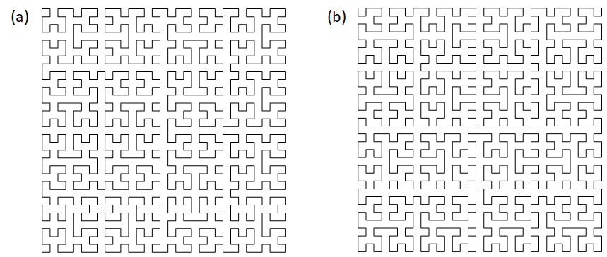
Given its fundamental shape of U, a Hilbert curve can be formed by placing the fundamental shape on the coarsest level (level 1) of a grid. For a Hilbert curve, the level one representation fits on a 2 by 2 grid, see Figure 1(a). Once the starting vertex is chosen (from either vertex with a valency of 1), the vertices are numbered as ones traverses the path. The numbering is not unique as the path could also be followed in the opposite direction. To form the level 2 Hilbert curve (on a 4 by 4 grid), the fundamental shape is centred on each vertex of the level 1 curve (Figure 1(b)) and rotated (Figure 1(c)) until the shapes can be linked with one another by connections (Figure 1(d)) that (i) are consistent with the discretisation stencil and (ii) result in a continuous curve. Here the stencil implied by the Hilbert curve’s fundamental shape has connections between horizontal and vertical nearest neighbours - known as a five point stencil and often used in solving differential equations. This process of locating the fundamental shape at vertices and rotating them until a continuous curve is found, is repeated until the desired level is reached. Neighbouring vertices on the space-filling curve in (d) will be close in the graph for level 2 shown in (e) but the reverse is not necessarily true. For example, vertices 2 and 15 in Figure 1(d) are not close on the space-filling curve but are close in the original graph in (e). To overcome potential inaccuracies caused by the disconnect between neighbouring vertices on the original graph, the generation of multiple space-filling curves is explored, the aim of which is that such vertices would be closer on a subsequent space-filling curve. More details are given about multiple space-filling curves throughout this section. As an example, two 2D Hilbert curves for a 32 by 32 grid can be seen in Figure 2; both are used to generate the results for the structured grid test cases that are presented later.
The approach we take to form space-filling curves for unstructured meshes is similar to the above. For the fundamental shape, we choose a straight line (two vertices and one edge). The two vertices represent two partitions and the edge between them represents an edge on the original graph which connects them. Generating a space-filling curve consists of three steps. First, the graph is constructed, based on the discretisation stencil associated with the nodes or cells of the mesh. In the graph, vertices represent the nodes or cells, and edges represent the connections between nodes or cells as determined by the stencil. We refer to this as the ‘original graph’ to distinguish it from graphs of the partitions at intermediate levels of decomposition. Second, a hierarchy of partitions (and graphs) are created from the original graph using a domain decomposition approach based on nested bisection. The graph partitioner will be explained in the next section, but, important here is that it generates a series of partitions at different levels of refinement. Third, the partitions are ordered, beginning at the coarsest level and ending at the final level. Once complete, the space-filling curve ordering is obtained, either directly from the vertex ordering of the final level, or after an additional step if there is more than one vertex in any of the partitions.
The starting point for generating the space-filling curve ordering or numbering is therefore a hierarchy of nested partitions. As a consequence of the fundamental shape, at level 1, the coarsest level, there will be two partitions; at level 2, there will be 4 partitions; at level there will be partitions and so on. In addition to the original graph, at every level a graph of the partitions and their connectivities is constructed, from which the numbering is calculated. The method is now illustrated with reference to an example shown in Figure 3. Here, a 2D linear Finite Element (FE) discretisation is assumed which uses three-noded elements. The original graph of the computational domain and discretisation can be seen in Figure 3(a), which, for this stencil, coincides with the FE mesh. Based on the original graph (a), partitions at three levels, seen in (c), (e) and (g) respectively, are obtained from the graph partitioner. For each level, the ordering algorithm constructs a graph to represent the partitions and their connections seen in (d), (f), and (h). For level 1, the graph shown in (d) consists of two vertices (one in each partition) joined by an edge. The vertices in partitions and can be numbered arbitrarily as these partitions have the same parent and will be connected by an edge on the original graph. Once the vertices are numbered, the partitions are renumbered to be consistent with the vertex numbering, i.e. so that vertex is located in partition . For level 2, the first partition from level 1 () gives rise to partitions and , and the second partition from level 1 gives rise to and . Partitions and will be connected by an edge on the original graph, as will partitions and , for the reason that they share the same parent partition. What must be found is the connection between either or , and or . Incorporating this edge into the space-filling curve gives it continuity, and ideally, therefore, there would be just one edge needed to move from or to or . This is so the path traced out by the space-filling curve traverses the vertices in as efficient a manner as possible (given the stencil). At this level, there are four possible ways of numbering the vertices, resulting in four different paths through the graph. All combinations of numbering are tried and, for each, a functional is evaluated to find the best path or any one of the best paths. If one combination gives either the same value or an improved functional value, it is accepted. The functional is defined as the number of edges traversed in order to move from the first vertex to the fourth. In Figure 4 we show the four possible combinations of numbering, also shown in Table 1 along with the corresponding functional values. In Figure 4(a) the vertices are ordered according to the partition number, which produces a path with 3 edges. Vertices 1 and 2 are swapped in Figure 4(b) and the number of edges in the path from vertex 1 to 4 is 4. This path is rejected as the functional value has not reduced. Vertices 3 and 4 are swapped in Figure 4(c) producing a path of 3 edges which is accepted. Finally vertices 1 and 2 are swapped back, shown in Figure 4(d), also producing a path of 3 edges which is accepted. This is chosen as the final path and the partition numbers are updated to match the vertex numbers, shown in Figure 3(f).
| path | Figure | ||||||||
|---|---|---|---|---|---|---|---|---|---|
| vertex ordering | 1 | 2 | 3 | 4 | 3 | accepted | 4(a) | ||
| 2 | 1 | 3 | 4 | 4 | not accepted | 4(b) | |||
| 2 | 1 | 4 | 3 | 3 | accepted | 4(c) | |||
| 1 | 2 | 4 | 3 | 3 | accepted | 4(d) |
For level 3, there are 8 partitions, see Figure 3(g). The graph for this level can be seen in Figure 3(h). At this stage, there is only one vertex in each partition, so the graph resembles the FE mesh. As the number of vertices increases, the number of combinations grows exponentially, so at level 3, if the entire path is considered, that would result in 16 possible orderings. Instead of considering all the partitions simultaneously, groups of 4 partitions are considered in turn, as shown in Table 2. First, the four combinations of ordering the vertices in partitions 1 to 4 are considered by evaluating the functional from vertex 1 to 4, . Once the optimal ordering of these vertices has been found, vertices 1 and 2 are fixed and the vertices in partitions 3 to 6 are considered. The functional is now evaluated from the second to the sixth vertex, as the location of the third vertex relative to the second will affect the optimality of the path. When the ordering has been found, vertices 3 and 4 are fixed and now the vertices in partitions 5 to 8 are considered. The algorithm sweeps forwards and backwards through the partitions, considering four vertices at a time and fixing pairs of vertices based on the optimal path calculated between the appropriate number of vertices (4, 5 or 6) depending on whether the vertices either-side of the path have been fixed (see Table 2). For simple cases, only a small number of iterations are sufficient. For complex cases, more iterations are likely to be needed. In any case, it is not known whether the entire path from vertex 1 to vertex ( is the total number of vertices or nodes in the graph) produced by this method will be optimal, however, using 10 forwards and backwards ‘sweeps’ was found to be sufficient for the challenging example of an unstructured mesh with a discontinuous Galerkin stencil. Once the final level is reached, if there are multiple vertices in a partition, a series of vertex swapping operations are performed until an optimal path is found within that partition: that is a fully-connected path that links to the surrounding partitions and which has the shortest path. Hence, the space-filling curve ordering is obtained, of which, one possible solution is shown in Figure 3(b)
| 1 | 2 | 3 | 4 | 5 | 6 | 7 | 8 | ||||
| 2 | 1 | 3 | 4 | ||||||||
| 1 | 2 | 4 | 3 | ||||||||
| … forward sweep … | 2 | 1 | 4 | 3 | |||||||
| 2 | 1 | 4 | 3 | 5 | 6 | 7 | 8 | ||||
| 3 | 4 | 5 | 6 | ||||||||
| 3 | 4 | 6 | 5 | ||||||||
| 4 | 3 | 6 | 5 | ||||||||
| 2 | 1 | 4 | 3 | 5 | 6 | 7 | 8 | ||||
| 6 | 5 | 7 | 8 | ||||||||
| 6 | 5 | 8 | 7 | ||||||||
| … backward sweep … | 5 | 6 | 8 | 7 | |||||||
| 2 | 1 | 4 | 3 | 5 | 6 | 8 | 7 | ||||
| 3 | 4 | 5 | 6 | ||||||||
| 3 | 4 | 6 | 5 | ||||||||
| 4 | 3 | 6 | 5 | ||||||||
| 2 | 1 | 4 | 3 | 6 | 5 | 8 | 7 | ||||
| 1 | 2 | 4 | 3 | ||||||||
| 1 | 2 | 3 | 4 | ||||||||
| 2 | 1 | 3 | 4 |
This method of generating space-filling curves is applied to an structured grid and the resulting space-filling curve is shown in Figure 6. The graph for the grid was generated by assuming a 5 point finite-difference stencil: the same stencil that was used to generate the graph seen in Figure 1(e). In Figure 6 it can be seen that a satisfactory space-filling curve has been found for the grid, whilst using a method that can be applied to fully unstructured meshes. The curve found here has four instances where the path is longer than it needs to be (indicated by the diagonal lines). However, this path is close to optimal and deemed good enough for use here. For this grid, a Hilbert curve would represent an optimal solution. The number of edges traversed by the Hilbert curve would be 63. Our method returns a value of 67 as every diagonal line would count as two edges traversed on the stencil.
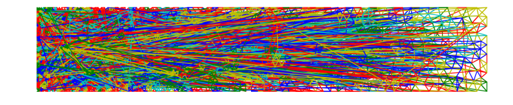
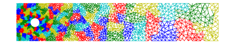
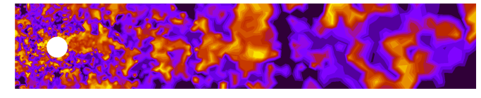
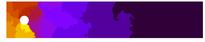
The discontinuous Galerkin (DG) discretisation has a particularly complex stencil (and graph) associated with it, see Figure 6 for the stencil associated with one node. For a DG node in element , this node is connected (through the stencil) to all nodes in element and all nodes in elements which share an edge (2D) or face (3D) with element . The edges for the node shown in Figure 6 would be constructed by drawing a line from the this node to each other green node. To draw the graph for the entire mesh shown here, this process would need to be done for every node in the mesh. The result of applying this method to an unstructured mesh can be seen in Figure 7, where a linear DG finite element stencil is used. There are 20,550 DG nodes in this mesh and 6,850 elements. In the top plots of this figure (top left and right), we show the path linking the first 200 DG nodes in one colour. The path connecting the next 200 DG nodes are plotted with another colour and so on. The plot on the left uses the node ordering as dictated by the meshing software, the plot on the right uses the node ordering provided by the space-filling curve. The ability of the space-filling curve to group together neighbouring nodes is clearly demonstrated. By grouping 200 DG nodes together in this way, a coarse-mesh representation of the problem is formed, illustrating one of the key reasons why combining space-filling curves and convolutional networks is so effective. The top right plot in Figure 7 could be interpreted as coarsening of the finite element mesh. Suppose that one level of coarsening was applied by taking every 4th node along the space-filling curve (reducing by a factor of 2 in each dimension), and this was done 4 times, then this is equivalent to taking every 256th node. Therefore, one could say the coarsening shown in this plot, by colouring groups of 200 DG nodes, is similar to applying 4 levels of coarsening which reduces the resolution by a factor 2 in each dimension (as 200256), which is similar to applying 4 convolutional layers with a stride of 2 for each dimension. The lower plots in Figure 7 show contour plots of the node numbers, with low numbers in black through to the highest node numbers in yellow. The plot on the left corresponds to the default node numbering based on the numbering provided by the meshing software, and the plot on the right corresponds to the node numbering from the space-filling curve.
2.2 Partitioning method
Many problems can be abstracted to the partitioning of a graph, such as the decomposition of computational domains, social network problems and travel network problems. Therefore much effort has been applied to the fundamental challenge of developing a method which simultaneously achieves an equal distribution of vertices/load between the partitions whilst minimising communication between partitions. A comprehensive survey of methods can be found here [42], which include spectral partitioning, geometric partitioning [43], multi-grid methods [18], methods based on the mean-field theorem [44], and also nested bisection approaches [45, 46, 47], which have seen success for partitioning large graphs.
A recurrent neural network based on mean-field theory (MFT-RNN) [48] is chosen to be the graph partitioner for the current work, as it (i) has a facility to set variable edge weights in the graph and (ii) can balance exactly (as far as possible) the number of vertices in each partition at each level. When generating multiple space-filling curves, there is a need to avoid cutting certain edges in the graph, so that different space-filling curves traverse distinct paths through the graph; which leads to the first requirement. The second requirement arises from the desire to obtain a final set of partitions, of which as many as possible contain at most one vertex. Partitions with more than one vertex can be dealt with, as can empty partitions, but the performance of the space-filling curve numbering algorithm will suffer in the former case. This multi-grid partitioning approach forms a hierarchy or nested sequence of partitions akin to that seen in multi-grid finite element methods [48, 18]. Other graph partitioning methods could be used as long as properties (i) and (ii) are attainable, such as methods that use vertex agglomeration by repeatedly merging adjacent vertices in a similar approach to multi-grid agglomeration methods [18].
More details of the MFT-RNN partitioner can be found in [48], however the main points are given here, along with details of the modifications made when generating multiple space-filling curves. The number of partitions created at each level is represented by , which, for the particular fundamental shape used in this paper, is necessarily . This recurrent neural network associates neurons with each vertex in the graph (i.e. one neuron for each desired partition), whose values represent the probability that a vertex is in partition :
| (1) |
The constraint has led to this method being referred to as normalised mean-field theory. For each partition, a vector of probabilities can be defined as
| (2) |
where is the number of vertices in the graph. For the special case of , only one neuron need be included for every vertex, as, given the probability of the vertex being in one partition, the probability of being the other can be calculated directly from the constraint. However, the code used to generate the examples in this paper was written only for the general case. Representing the quality of the partitions, the functional comprises two terms: the first describes the communication cost between vertices in different (proposed) partitions and the second describes how well the vertices are distributed between the partitions. It is written as follows:
| (3) |
where , and the scalar controls the balance between the importance of the distribution of vertices throughout the partitions and the importance of reducing the communication costs. The matrices and represent communication costs and balancing respectively, and are now explained in detail. The matrix consists of sub-matrices for partition numbers and , where . For , the sub-matrices consist entirely of zeros. For , the entries of the sub-matrices are defined as
| (4) |
The value represents the cost of vertex communicating with vertex and as well as determining the communication cost in the functional, this value is also taken as the th edge weight in the graph. When generating one space-filling curve, . When generating more than one space-filling curve, this parameter is set as
| (5) |
where the heuristically obtained exponent is set to be 0.2 and is the new space-filling curve node numbering of the th vertex in any one of the pre-existing space-filling curves labelled by . The idea behind introducing variable edge weights to the graph is to inject a means with which to discourage the graph to partition across edges that have large differences in space-filling curve numbers. This helps to ensure that a subsequent space-filling curve will avoid edges traversed by pre-existing curves, and encourages subsequent space-filling curves to find previously undiscovered paths through the graph. So, if two points are far apart on the first space-filling curve but close in Cartesian space, a second space-filling curve will attempt to find a path on which these points are closer.
Similar to , the matrix consists of sub-matrices for partition numbers and , where . To balance the vertices equally between the partitions (as far as possible), a diffusion matrix is used, the entries of which are defined as
| (6) |
for all partition numbers and for all vertices . In order to balance the number of vertices in each of the partitions at a particular level, the probabilities of vertex belonging to partition are exploited. If there is a need to transfer some vertices from one partition to another, the most suitable neurons are chosen from other partitions according to their probabilities. In this way, the uncertainty near the partition boundaries of the MFT-RNN is exploited, and thus, good quality partitions are maintained as well as near perfect balance of vertices in each partition.
The two terms in the functional tends to compete against one another during optimisation, so it is generally advantageous to set as small as possible, although just large enough so that the vertices are equally distributed between the partitions. If the value of is too large, the partitions will have equal numbers of vertices but the path traced out by the space-filling curve will not be as continuous as it could have been, resulting in a poor space-filling curve. In this paper, an optimised value of is used as derived in [48]:
| (7) |
Extensive numerical experiments have shown that the value of obtained from this equation results in good load balancing as well as good quality partitioning that minimises the sum of the weights between the different partitions.
In summary, the graph partitioning algorithm takes a graph and decomposes this into partitions, using a nested bisection approach. This continues until almost all of the partitions contain one vertex. This is done by calculating the number of levels of decomposition, , by finding the smallest integer that satisfies
| (8) |
The functional, Equation (3), is minimised using the neural network updating algorithm associated with the MFT neural network as described in [48] to obtain the desired graph partitioning. No training of this network is required as the weights are determined by the functional. The space-filling curve can now be constructed from the numbered partitions.
2.3 Multiple space-filling curves
One problem with using the space-filling curve approach is that there can be little connectivity between certain regions of the domain, because although points close together on the space-filling curve are also close together in the physical space, the reverse is not true. A simple example of this can be seen in Figure 1(d), where vertices 2 and 15 are not close on the space-filling curve but are close in the original graph in (e). A possible remedy is to use more than one space-filling curve, where the second curve should be discouraged from having the same edges as the first. One way of achieving this is though the graph partitioning procedure, by weighting the graph edges as described in Equation (4). This effectively discourages partitions from being made across the same edges in the previous SFCs. Nothing else is needed as the edge weights determine the communication between areas of the domain in the any additional SFCs. An example of two space-filling curves is shown in Figure 8. The first SFC (left) is optimal in that it uses the minimum number of edges to traverse all the cells in the grid. The second SFC (centre) is less optimal, as it jumps to nodes that are not neighbours in the stencil, shown as curved or diagonal lines in (b). In order to do this, the SFC will pass through nodes and edges more than once. This is partly due to the small size of the example. However, from (c), the combination of the two space-filling curves is shown, which shows that all but one of the edges on the original graph (shown in Figure 1(e)) are connected and only three edges appear in both SFCs.
We have experimented with an alternative method, which deletes the edges of the first SFC from the original graph used by the graph partitioner. Subsequent SFCs will then be forced to find new paths through the mesh. With this method, the quality of the second and subsequent SFCs was not as good as with the previous method, possibly because it excessively reduced the number of graph edges available to subsequent SFCs.
We have also experimented with introducing a constraint on the second SFC so that this space-filling curve starts at the final node of the first SFC. In this way, the second SFC follows the first SFC resulting in a continuous curve, which is advantageous to the performance of the 1D CNN. This constraint could be introduced in the SFC algorithm, simply, by always ensuring that the first partition on each level of the nested bisection contains this node (that is, the end node of the first SFC). For three space-filling curves one adds a similar constraint to the third SFC so that it start at the node next to the final node of the second SFC. A possible disadvantage of using this start-end constraint is that it can compromise the quality of the second and subsequent SFCs, in terms of producing a continuous curve, as, once again, the options of the SFC algorithm are restricted. A second disadvantage is that the number of weights is greater when the SFCs are combined into one continuous curve. For a 2D data set with 2 SFCs, having two separate SFCs results in a factor of two saving, in terms of weights in the 1D convolutional layers for the same total number of channels. A similar saving is also obtained in terms of arithmetic operations. For 3D problems this approach results in a saving of 3 times the number of weights and approximately similar saving for the CPU requirements associated with the convolutional layers. Thus, we chose here to have separate SFCs in the SFC-based CNNs.
3 Architectures of the convolutional networks
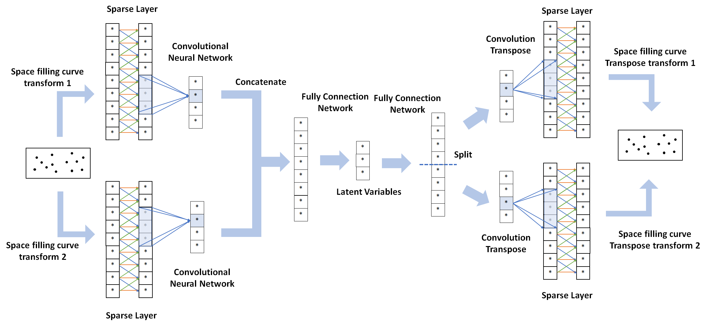
The architectures of the CNNs that will be used in the results section are described in detail in this section. To demonstrate the application of convolutional networks to data on both structured and unstructured meshes, a convolutional autoencoder is chosen. This type of network attempts to learn a compressed representation of data due to a bottleneck as its central layer. Consisting of an encoder and a decoder, the encoder compresses the data to a predetermined number of latent variables, known as the dimension of the latent space. The decoder reconstructs the data from the latent variables. For a convolutional autoencoder, the encoder has a number of convolutional layers typically followed by some fully-connected layers, and the decoder is the reverse of this.
In addition to the layers found in a classical convolutional autoencoder, the SFC-based convolutional autoencoders have: (1) a transformation from multi-dimensional data to 1D data and vice versa, based on SFCs; (2) sparse layers at either end of the network; and (3) nearest-neighbour smoothing (included in some of the networks). The transformation from multi-dimensional data to 1D data is determined by one or more space-filling curves and occurs in the first and final layers of the SFC-based autoencoders. Immediately after the first layer and before the final layer are the sparse layers. The function of the sparse layers is to apply some smoothing to the results and to decide the priority of the feature maps when recombining the data. The amount of smoothing provided by these layers can be increased by including a node’s nearest neighbours on the space-filling curve within the smoothing.
On transforming the multi-dimensional data to 1D data with the SFCs, there may be some associated CPU speed advantages as 1D arrays generally map straightforwardly onto the various memory hierarchies of modern CPUs or GPUs. This could make the SFC-based CNNs computationally faster than the classical multi-dimensional CNNs. However, we have found, through considerable trial and error, that it is necessary to use roughly uniform numbers of channels in the convolutional layers of the SFC-based networks. This is in contrast with the classical CNNs, which seem to work best when the number of channels increases in the encoder and decreases in the decoder. The more channels, the greater the computational speed and memory requirements, especially on layers with more neurons. Thus the classical CNN has a computational advantage over the SFC-based CNN in this regard.
To motivate the sparse layers further, consider a node on an SFC which is close in physical space to another node (or, more precisely, close on the graph associated with the discretisation stencil), but far away in terms of node numbering on the SFC. These nodes are disconnected, in some sense, which could potentially lead to a large variation in values occurring. This can result in discontinuities in the outputs from the autoencoder where there should be none. Having multiple SFCs allows such nodes to have low associated weights associated in the mapping to the final output layer, thus increasing the accuracy of the values of the output neurons. Therefore, for multiple space-filling curves, this layer can be thought of as a means of letting the network decide how to optimally combine results from two space-filling curves to form the final output result neural network. The transpose of this architecture is used for the encoder (as is often done with autoencoders). This effectively takes a weighted average of a node on a SFC with its two neighbouring nodes and forms another neuron from this as well as combining (in some optimal way) SFC results to form feature maps that are fed into the rest of the autoencoder.
The notation used to describe the networks is given in Section 3.1. In the subsequent sections, the autoencoders used in this paper are described in detail. For the structured data on a grid, we construct (1) a classical 2D autoencoder given in Section 3.2.1; (2) an autoencoder based on one space-filling curve described in Section 3.2.2; (3) an autoencoder based on two space-filling curves described in Section 3.2.3; (4) an autoencoder based on two space-filling curves with smoothing from the nearest neighbours given in Section 3.2.4. For the unstructured data, given on a mesh of 20,550 nodes, each with two velocity components, we construct (1) an autoencoder based on one space-filling curve with nearest-neighbour smoothing given in Section 3.3.1; and (2) an autoencoder based on two space-filling curves with nearest-neighbour smoothing described in Section 3.3.2.
3.1 Notation used to describe autoencoder architectures
The notation that describes the architecture of the convolutional autoencoders used in the following equations and in Tables 4, 5, 6 and 7 is explained. The layer ordering is described as L -[Type][SFC index][Component], where L refers to the layer number. ‘Type’ refers to how the data is stored and can be ‘GRID/grid’ (stored on an grid), ‘SFC/sfc’ (ordered by space-filling curve) or ‘FEM/fem’ (stored on a finite-element mesh). ‘SFC index’ indicates which SFC is being used (either 1 or 2 in our case) and ‘Component’ is an optional description, which, when compressing velocities, indicates that component as or . ‘Identity’ in the CNN tables refers to the use of no activation function (that is, the identity function itself) or simply mapping the data from the GRID/grid or FEM/fem representation to the SFC/sfc ordering or vice versa. A similar notation is used to indicate that the neurons are associated with either the GRID/grid, SFC/sfc or FEM/fem within the equations describing the neuron updates within the layers.
In the tables, ‘1 variable’ or ‘3 variables’ for the kernel size represents the identical operations (using kernel sizes of 1 or 3) to the standard filter approach except for the fact that the filter weights that applied to the neurons are not the same but vary for each neuron. The values are optimised as part of the training process. These filters are used to form the sparse layers, which apply smoothing of the SFC-based autoencoder solutions and increase the accuracy of these solutions. Each node in the output is determined by one or three nodes in the input (‘1 variable’ or ‘3 variables’). Connecting one node in the output with three nodes in the input is referred to here as nearest-neighbour smoothing. We call these sparse layers, because the number of parameters is much less than if the layers were fully connected. We have found their use to be essential in order to reduce the noise one would otherwise see in the SFC-based autoencoder results.
To identify neighbouring nodes in the SFC ordering, for layer and node number , we use to represent the neighbour (with an increase in SFC node number) of (that is ), and use to represent the neighbour (with a decrease in SFC node number) of (that is ).
3.2 Convolutional autoencoders for data on structured meshes
3.2.1 Architecture of a classical 2D convolutional autoencoder
Table 3 shows details of the classical 2D convolutional autoencoder applied to data on a structured grid. Layers 1 to 4 and 11 to 14 are convolutional layers, and the fully-connected layers are at the centre of the network, in layers 5 to 10. As is often done, the number of channels increases through the enocder and decreases through the decoder.
| layer | input size | kernel size | channels | stride | padding | output size | activation |
| 1 | (1, 128, 128) | 5 5 | 2 | 2 2 | 2 | (2, 64, 64) | ReLU |
| 2 | (2, 64, 64) | 5 5 | 4 | 2 2 | 2 | (4, 32, 32) | ReLU |
| 3 | (4, 32, 32) | 5 5 | 8 | 2 2 | 2 | (8, 16, 16) | ReLU |
| 4 | (8, 16, 16) | 5 5 | 16 | 2 2 | 2 | (16, 8, 8) | ReLU |
| Flatten the data to 1D, then use fully-connected layers to compress further | |||||||
| 5 | 1024 (= 1688) | 256 | ReLU | ||||
| 6 | 256 | 64 | ReLU | ||||
| 7 | 64 | 16 | ReLU | ||||
| 8 | 16 | 64 | ReLU | ||||
| 9 | 64 | 256 | ReLU | ||||
| 10 | 256 | 1024 | ReLU | ||||
| Convert data from 1024 to (16, 8, 8) then use convolutional layers to reconstruct the data | |||||||
| 11 | (16, 8, 8) | 5 5 | 8 | 2 2 | 2 | (8, 16, 16) | ReLU |
| 12 | (8, 16, 16) | 5 5 | 4 | 2 2 | 2 | (4, 32, 32) | ReLU |
| 13 | (4, 32, 32) | 5 5 | 2 | 2 2 | 2 | (2, 64, 64) | ReLU |
| 14 | (2, 64, 64) | 5 5 | 1 | 2 2 | 2 | (1, 128, 128) | ReLU |
3.2.2 Architecture of the convolutional autoencoder based on one space-filling curve
As shown in Table 4, the autoencoder based on one SFC first transforms the multi-dimensional data to 1D data with the space-filling curve ordering. After this, are the sparse layers (layers 1 and 2). Then follows a classical 1D convolutional autoencoder. At the output of this, there are more sparse layers (layers 17 and 18) followed by a transformation of the data from 1D to the original multi-dimensional form. Here we describe the sparse layers. The filters of the sparse layers are defined using weight vectors, as these filters change at each node. This results in an efficient implementation of the sparse layers. These weights effectively provide smoothing of the outputs of the SFC-based autoencoders, without which, would lead to noisy results.
Layers 1 and 2 (sparse layers)
The input, , is transformed using the Hilbert curve mapping to a 1D vector () in layer 1. Then the output of the sparse layer 2 is:
| (9) |
where is the weight vector (subject to neural network training), is the bias (again subject to training), is the ReLU activation function, and is the Hadamard product indicating entry-wise multiplication. Note that is the input for layer 3 of the neural network. See Table 4 for a description of the convolutional layers, which take input from layer 2.
| layer | input size | kernel size | channels | stride | padding | output size | activation |
| 1-GRID | (1, 16384, GRID) | 1 Identity | 1 | 1 | 0 | (1, 16384, SFC1) | Identity |
| 2-SFC1 | (1, 16384, SFC1) | 1 Variable (1 16384) | 1 | 1 | 0 | (1, 16384, SFC1) | ReLU |
| 3-SFC1 | (1, 16384, SFC1) | 32 | 2 | 4 | 16 | (2, 4097, SFC1) | ReLU |
| 4-SFC1 | (2, 4097, SFC1) | 32 | 4 | 4 | 16 | (4, 1025, SFC1) | ReLU |
| 5-SFC1 | (4, 1025, SFC1) | 32 | 8 | 4 | 16 | (8, 257, SFC1) | ReLU |
| 6-SFC1 | (8, 257, SFC1) | 32 | 16 | 4 | 16 | (16, 65, SFC1) | ReLU |
| Flatten the data to 1D, then use fully-connected layers to compress further | |||||||
| 7-SFC1 | 1040 (= 1665) | 256 | ReLU | ||||
| 8-SFC1 | 256 | 64 | ReLU | ||||
| 9-SFC1 | 64 | 16 | ReLU | ||||
| 10-SFC1 | 16 | 64 | ReLU | ||||
| 11-SFC1 | 64 | 256 | ReLU | ||||
| 12-SFC1 | 256 | 1024 | ReLU | ||||
| Convert data from 1024 to (16, 64, SFC1) then use convolutional layers to reconstruct the data | |||||||
| 13-SFC1 | (16, 64, SFC1) | 32 | 8 | 4 | 14 | (8, 256, SFC1) | ReLU |
| 14-SFC1 | (8, 256, SFC1) | 32 | 4 | 4 | 14 | (4, 1024, SFC1) | ReLU |
| 15-SFC1 | (4, 1024, SFC1) | 32 | 2 | 4 | 14 | (2, 4096, SFC1) | ReLU |
| 16-SFC1 | (2, 4096, SFC1) | 32 | 1 | 4 | 14 | (1, 16384, SFC1) | ReLU |
| 17-SFC1 | (1, 16384, SFC1) | 1 Variable (1 16384) | 1 | 1 | 0 | (1, 16384, SFC1) | Identity |
| 18-SFC1 | (1, 16384, SFC1) | 1 Identity | 1 | 1 | 0 | (1, 16384, GRID) | ReLU |
Layers 17 and 18 (sparse layers)
Given the input , the output of the sparse layer 17 (which is the final output of the SFC-based CNN) can be written as:
| (10) |
where is the weight vector, is the bias, and is the ReLU activation function. Using the inverse space-filling curve mapping, the 1D data, , is transformed back to 2D data on the structured grid, .
3.2.3 Architecture of a convolutional autoencoder based on two space-filling curves
The architecture of autoencoder based on two space-filling curves is given in Table 5. When using two space-filling curves, we keep the neuron values associated with these curves separate in the convolutional layers, but bring this information together within the fully-connected laters at the centre, as well as the input and output layers. The sparse layers are now described in detail.
Layers 1 and 2 (sparse layers)
The data on the grid, , is transformed to two 1D vectors using the mappings from the two space-filling curves to produce in layer 1. The output of the sparse layer 2 is:
| (11) |
| (12) |
where are the weight vectors, are the bias vectors, and is the ReLU activation function. The input for layer 3 takes the form . See Table 5 for a description of the following convolutional layers of the network.
Layers 18 and 19 (sparse layers)
Given the inputs and , the output of the sparse layer 18 is:
| (13) |
| (14) |
where are the weight vectors. Using the inverse mappings from the first and second space-filling curves, the vectors and are transformed to obtain and . Added to this is the bias . The output of the network is and is obtained from:
| (15) |
in which is the ReLU activation function.
| layer ordering | input size & ordering | kernel size | channels | stride | padding | output size & ordering | activation |
| 1-GRID | (1, 16384, GRID) | 1 Identity | 1 | 1 | 0 | (1, 16384, SFC1) | Identity |
| 2-SFC1 | (1, 16384, SFC1) | 1 Variable () | 2 | 1 | 0 | (1, 16384, SFC1) | ReLU |
| 3-SFC1 | (1, 16384, SFC1) | 32 | 2 | 4 | 16 | (2, 4097, SFC1) | ReLU |
| 4-SFC1 | (2, 4097, SFC1) | 32 | 4 | 4 | 16 | (4, 1025, SFC1) | ReLU |
| 5-SFC1 | (4, 1025, SFC1) | 32 | 8 | 4 | 16 | (8, 257, SFC1) | ReLU |
| 6-SFC1 | (8, 257, SFC1) | 32 | 16 | 4 | 16 | (16, 65, SFC1) | ReLU |
| 1-GRID | (1, 16384, GRID) | 1 Identity | 1 | 1 | 0 | (1, 16384, SFC2) | Identity |
| 2-SFC2 | (1, 16384) | 1 Variable () | 1 | 1 | 0 | (1, 16384, SFC2) | ReLU |
| 3-SFC2 | (1, 16384) | 32 | 2 | 4 | 16 | (2, 4097, SFC2) | ReLU |
| 4-SFC2 | (2, 4097) | 32 | 4 | 4 | 16 | (4, 1025, SFC2) | ReLU |
| 5-SFC2 | (4, 1025) | 32 | 8 | 4 | 16 | (8, 257, SFC2) | ReLU |
| 6-SFC2 | (8, 257) | 32 | 16 | 4 | 16 | (16, 65, SFC2) | ReLU |
| Flatten the output data of layer 6-SFC1 and 6-SFC2 to 1D - concatenate 2 sequences | |||||||
| 7 | 2080 (= 1665 + 1665) | 512 | ReLU | ||||
| 8 | 512 | 128 | ReLU | ||||
| 9 | 128 | 16 | ReLU | ||||
| 10 | 16 | 128 | ReLU | ||||
| 11 | 128 | 512 | ReLU | ||||
| 12 | 512 | 2048 | ReLU | ||||
| Split the data into 2 sequence as the input of layer 11-SFC1 and 11-SFC2, convert from 1024 to (16, 64) | |||||||
| 13-SFC1 | (16, 64, SFC1) | 32 | 8 | 4 | 14 | (8, 256, SFC1) | ReLU |
| 14-SFC1 | (8, 256, SFC1) | 32 | 4 | 4 | 14 | (4, 1024, SFC1) | ReLU |
| 15-SFC1 | (4, 1024, SFC1) | 32 | 2 | 4 | 14 | (2, 4096, SFC1) | ReLU |
| 16-SFC1 | (2, 4096, SFC1) | 32 | 1 | 4 | 14 | (1, 16384, SFC1) | ReLU |
| 17-SFC1 | (2, 16384, SFC1) | 1 Variable () | 1 | 1 | 0 | (1, 16384, SFC1) | Identity |
| 18-SFC1 | (1, 16384, SFC1) | 1 Identity | 1 | 1 | 0 | (1, 16384, GRID1) | Identity |
| 13-SFC2 | (16, 64, SFC2) | 32 | 8 | 4 | 14 | (8, 256, SFC2) | ReLU |
| 14-SFC2 | (8, 256, SFC2) | 32 | 4 | 4 | 14 | (4, 1024, SFC2) | ReLU |
| 15-SFC2 | (4, 1024, SFC2) | 32 | 2 | 4 | 14 | (2, 4096, SFC2) | ReLU |
| 16-SFC2 | (2, 4096, SFC2) | 32 | 1 | 4 | 14 | (1, 16384, SFC2) | ReLU |
| 17-SFC2 | (2, 16384, SFC2) | 1 Variable () | 1 | 1 | 0 | (1, 16384, SFC2) | Identity |
| 18-SFC2 | (1, 16384, SFC2) | 1 Identity | 1 | 1 | 0 | (1, 16384, GRID2) | Identity |
| 19-GRID | (, 16384) | 1 Identity GRID1 + GRID2 | 1 | 1 | 0 | (1, 16384, GRID) | ReLU |
3.2.4 Architecture of a convolutional autoencoder based on two space-filling curves with nearest-neighbour smoothing
The only difference between this SFC-based CNN and the previous one is the introduction of the nearest neighbours in the sparse layers. This effectively reduces the noise in the output of the SFC-based CNN.
Layers 1 and 2 (sparse layers)
The input to the network, , is transformed to by the two space-filling curve mappings in layer 1. In SFC ordering, is the neighbour (with an increase in SFC node number) of , and is the neighbour (with an decrease in SFC node number) of , in which is the number of the SFC. The output of the sparse layer 2 is given as:
| (16) |
| (17) |
where are the weight vectors, , are the bias vectors, and is the ReLU activation function. The input to layer 3 is and . See Table 5 for a description of the convolutional layers.
Layers 18 and 19 (sparse layers)
Given the inputs , in the SFC ordering is the neighbour (with an increase in SFC node number) of , and is the neighbour (with an decrease in SFC node number) of . The output of layer 18 is:
| (18) |
| (19) |
where are the weight vectors. Using the inverse of both space-filling curve mappings, transform and to and respectively, then add the bias to obtain:
| (20) |
in which is the ReLU activation function and is the output of this SFC-based CNN on the original grid.
3.3 Architectures of convolutional autoencoders for data on unstructured meshes
3.3.1 An autoencoder based on one space-filling curve with nearest-neighbour smoothing
Since flow past a cylinder is a more demanding compression problem than the previous two idealised cases, two channels are used for the sparse layer filters. If only one channel were used to be used, as in the idealised cases, the SFC-based CNN outputs tended to be noisy. In addition, within the sparse layers, the velocity components and are kept separate, in order to reduce the number of weights required in these layers and also to apply the smoothing to the velocity components separately. These modifications to the CNN are also applied to the SFC-based CNN with two SFCs, also used for flow past a cylinder. See Table 5 for a description of this autoencoder. We now describe the sparse layers in detail.
Layers 1 and 2 (sparse layers)
The input to the neural network is and contains two channels; one for the first velocity component, , and the second for the other velocity component, . These are held in the FEM DG ordering of the nodal values of the velocities. The input, , is mapped to the SFC ordering, , using the SFC mapping in layer 1. By splitting the channels of , we obtain and , associated with the two velocity components respectively. In the SFC ordering, are the neighbours (with an increase in SFC node number) of (that is ), is the neighbour (with an decrease in SFC node number) of (that is ). The output of the sparse layer 2 is then:
| (21) | |||||
| (22) | |||||
where are the weight vectors, , are the bias vectors, and is the tanh activation function. Then:
| (23) |
where is the input for layer 3. The notation is used to represent the concatenation of two vectors into one, and the notation represents the concatenation of one vector with itself.
Layers 13, 14 and 15 (sparse layers)
The vector (in SFC ordering), is disconcatenated or split into two; . Similar to previously are the neighbours (with an increase in SFC node number) of , and are the neighbours (with a decrease in SFC node number) of . Thus:
| (24) |
| (25) |
where are the weight vectors and , . The operator simply adds together the vectors in each channel to produce a one-channel output. Using the inverse SFC mappings, and are then transformed to and in the original FEM mesh ordering. The output neurons in FEM ordering are:
| (26) |
in which is the bias, is the tanh activation function and the two channels of contain the and nodal velocity components, respectively, on the FEM DG mesh.
| layer | input size | kernel size | channels | stride | padding | output size | activation |
| 1-FEM | (2, 20550, FEM) | 1 Identity | 2 | 1 | 0 | (2, 20550, SFC1) | Identity |
| Split (2, 20550, SFC1) into two:(1, 20550, SFC1), (1, 20550, SFC1) | |||||||
| 2-SFC1 | (1, 20550, SFC1) | 3 Variable () | 2 | 1 | 0 | (2, 20550, SFC1) | tanh |
| 2-SFC1 | (1, 20550, SFC1) | 3 Variable () | 2 | 1 | 0 | (2, 20550, SFC1) | tanh |
| concatenate:((2, 20550, SFC1), (2, 20550, SFC1)) forming (4, 20550, SFC1) | |||||||
| 3-SFC1 | (4, 20550, SFC1) | 32 | 16 | 4 | 16 | (16, 5138, SFC1) | tanh |
| 4-SFC1 | (16, 5138, SFC1) | 32 | 16 | 4 | 16 | (16, 1285, SFC1) | tanh |
| 5-SFC1 | (16, 1285, SFC1) | 32 | 16 | 4 | 16 | (16, 322, SFC1) | tanh |
| 6-SFC1 | (16, 322, SFC1) | 32 | 16 | 4 | 16 | (16, 81, SFC1) | tanh |
| Flatten the output data of layer 6 to 1D | |||||||
| 7 | 1296 (= 1681) | 128 | tanh | ||||
| 8 | 128 | 1296 | tanh | ||||
| Convert from 1296 to (16, 81, SFC1) as the input of layer 9 | |||||||
| 9-SFC1 | (16, 81, SFC1) | 32 | 16 | 4 | 15 | (16, 322, SFC1) | tanh |
| 10-SFC1 | (16, 322, SFC1) | 32 | 16 | 4 | 15 | (16, 1286, SFC1) | tanh |
| 11-SFC1 | (16, 1286, SFC1) | 32 | 16 | 4 | 16 | (16, 5140, SFC1) | tanh |
| 12-SFC1 | (16, 5140, SFC1) | 32 | 4 | 4 | 19 | (4, 20550, SFC1) | tanh |
| Split (4, 20550, SFC1) into two:(2, 20550, SFC1), (2, 20550, SFC1) | |||||||
| 13-SFC1 | (2, 20550, SFC1) | 3 Variable () | 2 | 1 | 0 | (1, 20550, SFC1) | Identity |
| 13-SFC1 | (2, 20550, SFC1) | 3 Variable () | 2 | 1 | 0 | (1 20550, SFC1v) | Identity |
| 14-SFC1 | (1, 20550, SFC1) | 1 Identity | 1 | 1 | 0 | (1, 20550, FEM1u) | Identity |
| 14-SFC1 | (1, 20550, SFC1) | 1 Identity | 1 | 1 | 0 | (1, 20550, FEM1v) | Identity |
| 15-FEM | (, 20550, FEM) | 1 Identity (FEM1,FEM1) | 2 | 1 | 0 | (2, 20550, FEM) | tanh |
3.3.2 An autoencoder based on two space-filling curves with nearest-neighbour smoothing
Layers 1 and 2 (sparse layers)
Given the input , convert this to the SFC1 and SFC2 ordering using the SFC mappings in layer 1. By splitting the channels of and , we obtain for velocity components and respectively. The output of the sparse layer 2 is:
| (27) | |||||
| (28) | |||||
| (29) | |||||
| (30) | |||||
where are the weight vectors, are the bias vectors, , and is the tanh activation function. Then we use:
| (31) |
as the input for layer 3-SFC1, and
| (32) |
as the input for layer 3-SFC2. See Table 5 for a description of the following convolutional layers.
Layers 13, 14 and 15 (sparse layers)
The vector is split into , and similarly is split into , . In SFC ordering, are the neighbours (with an increase in SFC node number) of , and are the neighbours (with an decrease in SFC node number) of in which is the SFC number and indicated the velocity component. Thus:
| (33) |
| (34) |
| (35) |
| (36) |
where are the weight vectors and , ,, . Now convert and using the inverse of the first space-filling curve ordering to obtain and , and convert and using the inverse of the second space-filling curve to obtain and . Then the output of the network is obtained from:
| (37) |
in which is the tanh activation function, the biases are and the two channels in contain the and velocity components.
| layer ordering | input size & ordering | kernel size | channels | stride | padding | output size & ordering | activation |
| 1-FEM | (2, 20550, FEM) | 1 Identity | 2 | 1 | 0 | (2, 20550, SFC1) | Identity |
| Split (2, 20550, SFC1) into two:(1, 20550, SFC1), (1, 20550, SFC1) | |||||||
| 2-SFC1 | (1, 20550, SFC1) | 3 Variable () | 2 | 1 | 0 | (2, 20550, SFC1) | tanh |
| 2-SFC1v | (1, 20550, SFC1) | 3 Variable () | 2 | 1 | 0 | (2, 20550, SFC1) | tanh |
| concatenate:((2, 20550, SFC1), (2, 20550, SFC1)) forming (4, 20550, SFC1) | |||||||
| 3-SFC1 | (4, 20550, SFC1) | 32 | 8 | 4 | 16 | (8, 5138, SFC1) | tanh |
| 4-SFC1 | (8, 5138, SFC1) | 32 | 8 | 4 | 16 | (8, 1285, SFC1) | tanh |
| 5-SFC1 | (8, 1285, SFC1) | 32 | 8 | 4 | 16 | (8, 322, SFC1) | tanh |
| 6-SFC1 | (8, 322, SFC1) | 32 | 8 | 4 | 16 | (8, 81, SFC1) | tanh |
| 1-FEM | (2, 20550, FEM) | 1 Identity | 2 | 1 | 0 | (2, 20550, SFC2) | Identity |
| Split (2, 20550, SFC2) into two:(1, 20550, SFC2), (1, 20550, SFC2) | |||||||
| 2-SFC2 | (1, 20550) | 3 Variable () | 2 | 1 | 0 | (2, 20550, SFC2) | tanh |
| 2-SFC2 | (1, 20550) | 3 Variable () | 2 | 1 | 0 | (2, 20550, SFC2) | tanh |
| concatenate:((2, 20550, SFC2), (2, 20550, SFC2)) forming (4, 20550, SFC2) | |||||||
| 3-SFC2 | (4, 20550, SFC2) | 32 | 8 | 4 | 16 | (8, 5138, SFC2) | tanh |
| 4-SFC2 | (8, 5138, SFC2) | 32 | 8 | 4 | 16 | (8, 1285, SFC2) | tanh |
| 5-SFC2 | (8, 1285, SFC2) | 32 | 8 | 4 | 16 | (8, 322, SFC2) | tanh |
| 6-SFC2 | (8, 322, SFC2) | 32 | 8 | 4 | 16 | (8, 81, SFC2) | tanh |
| Flatten the output data of layer 6-SFC1 and 6-SFC2 to 1D - concatenate 2 sequences | |||||||
| 7 | 1296 (= 881 + 881) | 128 | tanh | ||||
| 8 | 128 | 1296 | tanh | ||||
| Split the data into 2 sequence as the input of layer 9-SFC1 and 9-SFC2, convert from 1296 to (8, 81) | |||||||
| 9-SFC1 | (8, 81, SFC1) | 32 | 8 | 4 | 15 | (8, 322, SFC1) | tanh |
| 10-SFC1 | (8, 322, SFC1) | 32 | 8 | 4 | 15 | (8, 1286, SFC1) | tanh |
| 11-SFC1 | (8, 1286, SFC1) | 32 | 8 | 4 | 16 | (8, 5140, SFC1) | tanh |
| 12-SFC1 | (8, 5140, SFC1) | 32 | 4 | 4 | 19 | (4, 20550, SFC1) | tanh |
| Split (4, 20550, SFC1) into two:(2, 20550, SFC1), (2, 20550, SFC1) | |||||||
| 13-SFC1 | (2, 20550, SFC1) | 3 Variable () | 2 | 1 | 0 | (1, 20550, SFC1) | Identity |
| 13-SFC1 | (2, 20550, SFC1) | 3 Variable () | 2 | 1 | 0 | (1, 20550, SFC1) | Identity |
| 14-SFC1 | (1, 20550, SFC1) | 1 Identity | 1 | 1 | 0 | (1, 20550, FEM1) | Identity |
| 14-SFC1 | (1, 20550, SFC1) | 1 Identity | 1 | 1 | 0 | (1, 20550, FEM1) | Identity |
| 9-SFC2 | (8, 81, SFC2) | 32 | 8 | 4 | 15 | (8, 322, SFC2) | tanh |
| 10-SFC2 | (8, 322, SFC2) | 32 | 8 | 4 | 15 | (8, 1286, SFC2) | tanh |
| 11-SFC2 | (8, 1286, SFC2) | 32 | 8 | 4 | 16 | (8, 5140, SFC2) | tanh |
| 12-SFC2 | (8, 5140, SFC2) | 32 | 4 | 4 | 19 | (4, 20550, SFC2) | tanh |
| Split (4, 20550, SFC2) into two:(2, 20550, SFC2), (2, 20550, SFC2) | |||||||
| 13-SFC2 | (2, 20550, SFC2) | 3 Variable () | 1 | 1 | 0 | (1, 20550, SFC2) | Identity |
| 13-SFC2 | (2, 20550, SFC2) | 3 Variable () | 1 | 1 | 0 | (1 20550, SFC2) | Identity |
| 14-SFC2 | (1, 20550, SFC2) | 1 Identity | 1 | 1 | 0 | (1, 20550, FEM2) | Identity |
| 14-SFC2 | (1, 20550, SFC2) | 1 Identity | 1 | 1 | 0 | (1, 20550, FEM2) | Identity |
| 15-FEM | (, 20550) | 1 Identity ((FEM1,FEM1)+(FEM2,FEM2)) | 2 | 1 | 0 | (2, 20550, FEM) | tanh |
4 Results
Three examples are used to demonstrate the potential of the method proposed in this paper, of applying convolutional networks to data held on any mesh (structured grids or unstructured meshes) by using space-filling curves. Two of the test cases consist of structured grid data; the first data set represents advection of a square wave and the second represents advection of a Gaussian function. The third example uses a data set consisting of solutions of 2D flow past a cylinder solved on an unstructured mesh.
Section 4.1 describes how results from an SVD will be compared with the SFC-based autoencoders, and describes the error measure used to compare the results. Section 4.2 defines some of the remaining hyper-parameters not defined in Section 3. Section 4.3 explains how the two structured-grid data sets are generated and then presents results for three autoencoders based on space-filling curves, a classical 2D autoencoder and an SVD. Section 4.4 describes generation of the results for flow past a cylinder, which make up the unstructured mesh data set. Results are presented for the two autoencoders based on space-filling curves and an SVD.
4.1 Analysis of results
4.1.1 Singular Value Decomposition
The results from the convolutional autoencoders developed in this paper are compared with results from singular value decomposition (SVD). For a matrix , where each column corresponds to a particular solution or example from the data set, and each row corresponds to a particular node or cell, the SVD is defined as
| (38) |
where is a diagonal matrix containing the singular values of given in descending order, and are the left- and right-singular vectors respectively, and the asterisk denotes the conjugate transpose. The square of each singular value indicates how much information is contained in the corresponding mode or basis function (column of ). A low-rank approximation of can be formed by retaining only the largest singular values, setting the remaining singular values to zero, and recalculating the product:
| (39) |
where the only non-zero terms in are the largest singular values from . Comparison is made between convolutional autoencoders which have a latent space of dimension and SVDs which have been truncated to singular values.
4.1.2 Measuring the error
To evaluate the error in the various autoencoder and SVD approaches, the mean square error is used:
| (40) |
in which is the number of input (or output variables), the number of nodes or cells for instance, is a particular solution or example taken from the data set, is the number of solutions or examples under consideration, and is the difference between the original solution and its approximation. For the autoencoder, the approximation is formed by encoding and decoding the solutions or examples. For the SVD, the solutions are assembled into a matrix to which SVD is applied. The truncation is performed and the low-rank approximation obtained. For the examples using structured grid data, the examples or solutions are scalar fields so Equation (40) can be applied directly. For the data set with examples on an unstructured mesh, the solutions are vector fields (velocities), so in this case, is defined to be the error in speed at the th node for the th example.
4.2 Hyper-parameters of the autoencoders
For each particular autoencoder, some of the hyper-parameters are specified in Section 3, including kernel size, number of channels, stride, padding, activation function, number of layers and number of neurons per layer. Other hyper-parameters are loss function, batch size, optimiser, learning rate and number of epochs, which are given here, except for the number of epochs which is stated in the results section where appropriate. Through tuning these hyper-parameters, we have optimised the neural networks within this work. Unless explicitly stated, it can be assumed that the values given in Table 8 are used for the SFC-based autoencoders.
| batch size | loss function | optimiser | learning rate | activation function | ||
|---|---|---|---|---|---|---|
| structured data | 64 | MSE | Adam | 0.0001 | ReLU | |
| unstructured data | 16 | MSE | Adam | 0.0001 | tanh |
The kernel size for the 2D classical autoencoder is with a stride of . To make the 1D SFC-based autoencoders approximately analagous to this, a kernel size of 32 is used with a stride of 4. A number of activation functions were experimented with, and ReLU and tanh performed the best. Here we use ReLU for the structured data and tanh for the unstructured data. All the input data for the autoencoders are normalised between for the structured data and for the unstructured data. The unstructured data has a larger computational cost associated with it, so the batch size was reduced from 64 to 16. The loss function chosen is the mean square error (MSE) given in Equation (40), and errors calculated using this formula are based on the normalised data values.
4.3 Structured Grid Applications
The generation of the data sets for the square wave and Gaussian function test cases is described. These data sets represent two extremes, from abruptly changing fields to smoothly changing fields. The performance of the new autoencoders based on space-filling curve ordering is analysed and comparisons are made with a classical 2D convolutional autoencoder (CAE) and SVD.
4.3.1 Generating square wave data
In order to generate data that represents advection of a square wave, the time-dependent 2D advection equation is solved:
| (41) |
in which represents time, and are the coordinates, is the concentration field and the advection velocity vector is given by . The discretisation method used to solve this equation is upwind differencing in space and the backward Euler method in time. The initial condition is given as:
| (42) |
and defined on the domain . For this problem, , , , . The domain is discretised using a uniform grid, the time step is and the variables and are chosen randomly from the interval . For this test case, the number of initial conditions created is , each generating time levels, so the total number of solutions or examples in the data set is 15360. The data is divided randomly into three parts according to the proportion 6:2:2, for training, validation and testing.
4.3.2 Generating the Gaussian data
To represent advection of a Gaussian function, the following profile is simply located at different points in the domain. The form of the Gaussian is given by
| (43) |
where represents the centre of the Gaussian function, whose values are randomly sampled from the domain, which is discretised with a structured grid. The parameter , which controls the width of the curve, is uniformly randomly sampled from the interval . The data set consists of a total examples.
4.3.3 Results for advection of a square wave
In order to assess their relative capabilities, we compare three SFC-based convolutional autoencoders, a classical 2D convolutional autoencoder and the SVD, all applied to the square wave data set. The autoencoders, their abbreviations and the section in which their architesctures are described, are listed in Table 9.
| abbreviation | architecture | description |
|---|---|---|
| CAE | Table 3, Section 3.2.1 | classical convolutional autoencoder |
| CAE-SFC | Table 4, Section 3.2.2 | a convolutional autoencoder based on ordering from one SFC |
| CAE-2SFC | Table 5, Section 3.2.3 | a convolutional autoencoder based on ordering from two SFCs |
| CAE-2SFC-NN | Section 3.2.4 | a convolutional autoencoder based on ordering from two SFCs and nearest-neighbour smoothing |
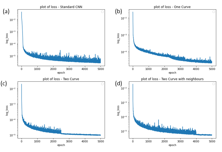
The convolutional autoencoders all compress to 16 latent variables having been trained over 5000 epochs and the SVD truncates to 16 variables. The so-called losses, defined here as the mean square error between the inputs and outputs of the autoencoder, see Equation (40), are shown in Figure 10 and Table 10, the latter includes the truncation error of the SVD. Both figure and table show that at 5000 epochs the losses of the classical 2D CAE and CAE-2SFC-NN are smaller than those of the CAE-SFC and CAE-2SFC autoencoders. All the autoencoders have a lower mean square error than the SVD.
| 2D CAE | CAE-SFC | CAE-2SFC | CAE-2SFC-NN | SVD |
|---|---|---|---|---|
Next, we investigate the effect of the dimension of the latent space by training two autoencoders to compress to both 16 and 8 latent variables. The best-performing SFC-based autoencoder from the previous results (CAE-SFC2-NN) is compared with the classical 2D CAE and the SVD. In training, 2000 epochs were used, and the losses for the training, validation and test data sets can be seen in Table 11. From this, it can be seen that the classical CAE performs a little better than CAE-2SFC-NN when compressing to 16 variables; both perform better than the SVD. However, the classical autoencoder struggles to converge when compressing to 8 variables. The CAE-2SFC-NN network performs well for both levels of compression presented here.
| 2D CAE | CAE-2SFC-NN | SVD | compression | |
|---|---|---|---|---|
| Training data | ||||
| Validation data | 16 | |||
| Test data | ||||
| Training data | ||||
| Validation data | 8 | |||
| Test data |
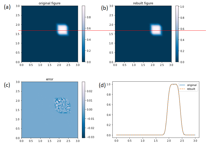
For one example, Figure 11 shows the performance of the autoencoder based on two SFCs with nearest-neighbour smoothing (CAE-2SFC-NN), which compresses to 16 latent variables and was trained in 5000 epochs. It can be seen that the network performs well and accurately reproduces the profile of the demanding square wave function. Plot (a) and (b) show the square wave solution before and after the application of the autoencoder respectively. The red line indicates a height of 1.7, at which plot (d) compares the original solution with the output of the autoencoder. Plot (c) shows the pointwise error, which, has an absolute value of, at most, 3%.
We also used a finer grid, , to compare the classical 2D CAE and the CAE-2SFC-NN autoencoder for the square wave data set, see Table 12 for the losses. The classical CAE does not converge on this finer grid, with a loss similar in magnitude to the truncation error of the SVD, but the CAE-2SFC-NN autoencoder converges well.
| classical CAE | CAE-2SFC-NN | SVD | |
|---|---|---|---|
| Training data | |||
| Validation data | |||
| Test data |
4.3.4 Results for advection of a Gaussian function
In this section, the architectures are the same as those used in the previous section for the advection of a square wave, as the grid is the same size. First, the performance of the autoencoder based on two SFCs with nearest-neighbour smoothing is compared with the classical CAE and the SVD. The autoencoders are both compressed to 16 and 8 variables, and trained for 2000 epochs. The SVD is truncated to 16 and 8 variables. The losses are given in Table 13, from which it can be seen that the autoencoder based on two SFCs with nearest-neighbour smoothing performs a little better than the classical autoencoder, and both are considerably better than the SVD when compressing to 16 variables. However, the classical convolutional autoencoder cannot converge when compressing to 8 variables.
| 2D CAE | CAE-2SFC-NN | SVD | compression | |
|---|---|---|---|---|
| Training data | ||||
| Validation data | 16 | |||
| Test data | ||||
| Training data | ||||
| Validation data | 8 | |||
| Test data |
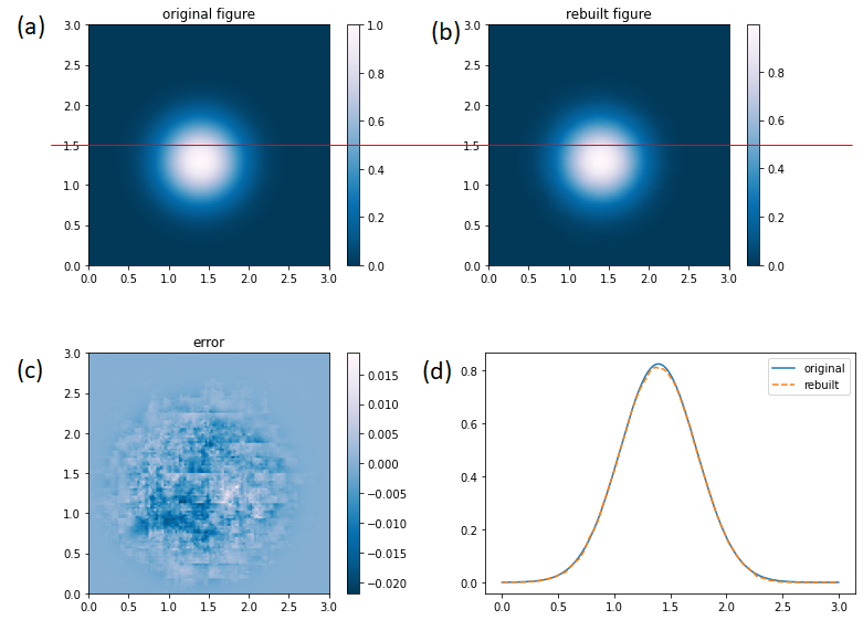
For one solution, Figure 12 shows the solution (a) before and (b) after being passed through the autoencoder (CAE-2SFC-NN). It can be seen that that the model performs well and accurately reproduces the smooth Gaussian function for this particular example. Plot (c) shows the pointwise error, which, at most, has an absolute value of 2%. Plot (d) compares the original solution with the output of the autoencoder at a height of 1.5. The profiles shown are in very close agreement.
The SFC-based autoencoder with two SFCs and nearest-neighbour smoothing is also compared with the classical CAE and SVD for a data set generated on a finer grid of . The losses are shown in Table 14. Here we see that, as for the square wave data set (Table 12), the classical CAE does not converge for the Gaussian function data set but the new CAE-2SFC-NN does converge. The data was compressed to 16 variables and the networks trained over 1000 epochs. We thus conclude that the new SFC-based autoencoder has comparable (possibly slightly better) accuracy to the classical 2D convolutional autoencoder; it outperforms the SVD (for these low dimensional spaces); it converges for a wider range of problems; but most importantly, the SFC-based autoencoders can be applied to data from unstructured meshes.
| 2D CAE | CAE-2SFC-NN | SVD | |
|---|---|---|---|
| Training data | |||
| Validation data | |||
| Test data |
4.4 Unstructured mesh test case
A data set consisting of solutions for 2D flow past a cylinder is created. These results lie on an unstructured mesh which will reveal the effectiveness of the method for this type of data. The SFC-based approach is compared with the SVD.
4.4.1 Results for 2D flow past a cylinder
Using the conservation laws, the following system of partial differential equations governing the motion of an incompressible fluid is obtained:
| (44) | |||||
| (45) |
where is the density (assumed constant), is the velocity vector, contains the viscous terms associated with an isotropic Newtonian fluid, represents the non-hydrostatic pressure, is time and the gradient operator is defined as
| (46) |
This system of equations is solved as outlined in [8]. For the discretisation, a linear triangular element is adopted with a discontinuous Galerkin discretisation of the velocities and a continuous Galerkin representation of the pressure, often referred to as the P1DG-P1 element. Crank Nicolson is used to discretise in time. Only velocity variables are needed to train the networks, as these fully describe incompressible flow. The Reynolds number for this problem is
| (47) |
in which the inlet velocity is constant, , the density has value and the diameter of the cylinder is . Thus the dynamic viscosity is . The domain measures horizontally, vertically, and the centre of the cylinder is located from the left boundary on the horizontal centreline of the domain. No slip and no normal flow boundary conditions are applied on the upper and lower walls, and on the cylinder. Zero shear and zero normal stress are applied at the outlet (the right boundary of the domain). In the following results, time is given in seconds, and speeds and velocities are in metres per second.
The data set, formed from the solutions of the above problem, consists of snapshots. Each snapshot has nodes, and each node has features (the two velocity components, and , in this two-dimensional problem). The data set is divided randomly (in the dimension) into three parts according to the proportion 8:1:1 for training, validation and testing.
First, in order to determine the effectiveness of multiple SFCs, comparison is made between two SFC-based convolutional autoencoders: one using one space-filling curve and the other using two space-filling curves. Both have nearest-neighbour smoothing. Following this, the performance of the CAE-2SFC-NN network is investigated for different dimensions of latent space. The architectures of the autoencoders are described in the sections and tables listed in Table 15.
| abbreviation | architecture | description |
|---|---|---|
| CAE-SFC-NN | Table 6, Section 3.3.1 | a convolutional autoencoder based on ordering from one SFC with nearest-neighbour smoothing |
| CAE-2SFC-NN | Table 7, Section 3.3.2 | a convolutional autoencoder based on ordering from two SFCs with nearest-neighbour smoothing |
4.4.2 Comparison between two SFC-based autoencoders
Figure 13 and Table 16 show the losses of the two SFC-based autoencoders, one using one space-filling curve and nearest-neighbour smoothing (CAE-SFC-NN), and the other using two space-filling curves and nearest-neighbour smoothing (CAE-2SFC-NN). Judging from the losses, the network that performs slightly better is the autoencoder based on two SFCs, despite the fact that the number of weights in the convolutional layers for this network is approximately half that of the autoencoder with one SFC (CAE-SFC-NN). The reason for its effectiveness is that the two space-filling curves attempt to capture features in all directions across the mesh as the curves sample two different directions (each curve is very roughly orthogonal to the other) at a given node in the mesh. The compression accuracy of the two networks can be seen in Figure 14 and are both impressive. On careful inspection of the results based on one SFC, in Figure 14 (upper plots), one can see that they are noisier than the results based on two SFCs (lower plots), which highlights a possible advantage of two SFCs leading to more accurate results. However, the network based on one SFC (CAE-SFC-NN) still represents the basic flow features very well.
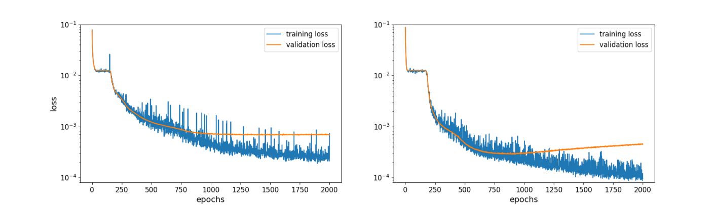
| CAE-SFC-NN | CAE-2SFC-NN | |
|---|---|---|
| Training data | ||
| Validation data | ||
| Test data |
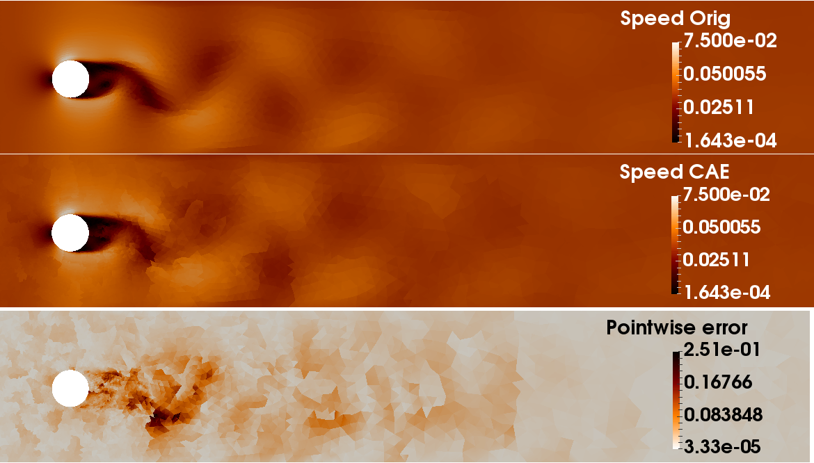
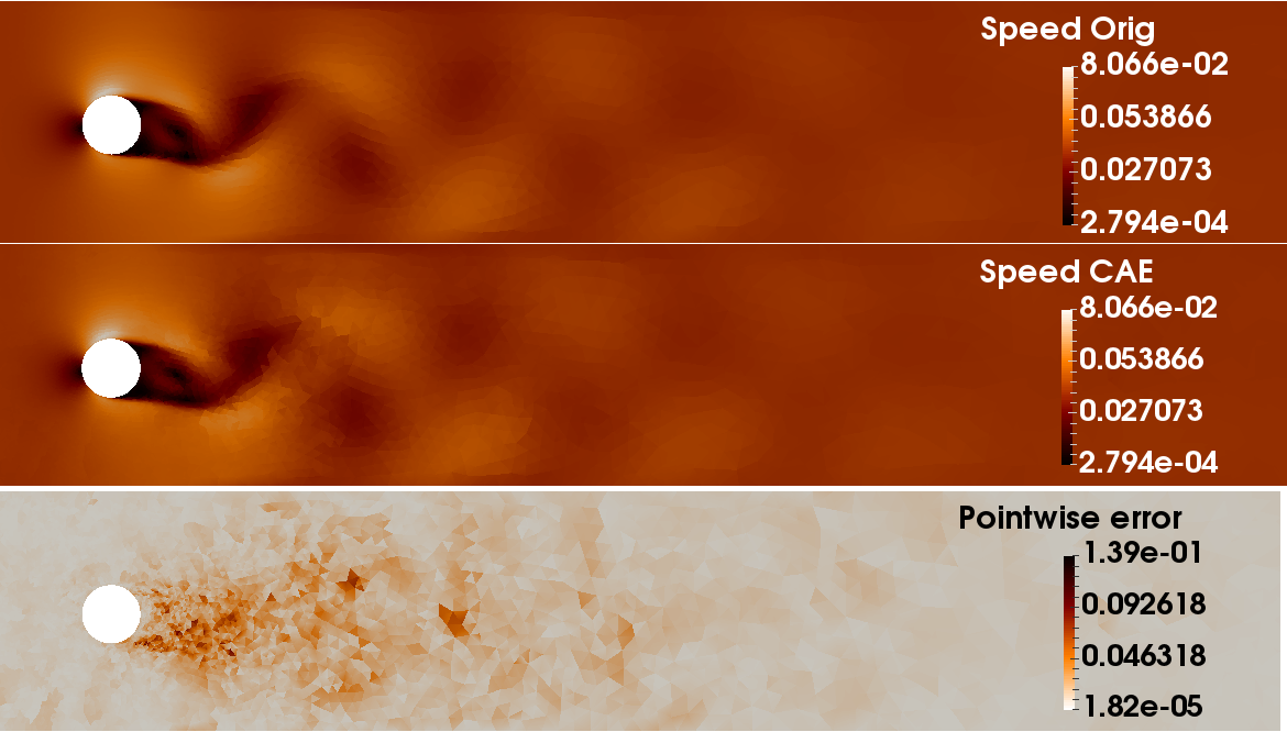
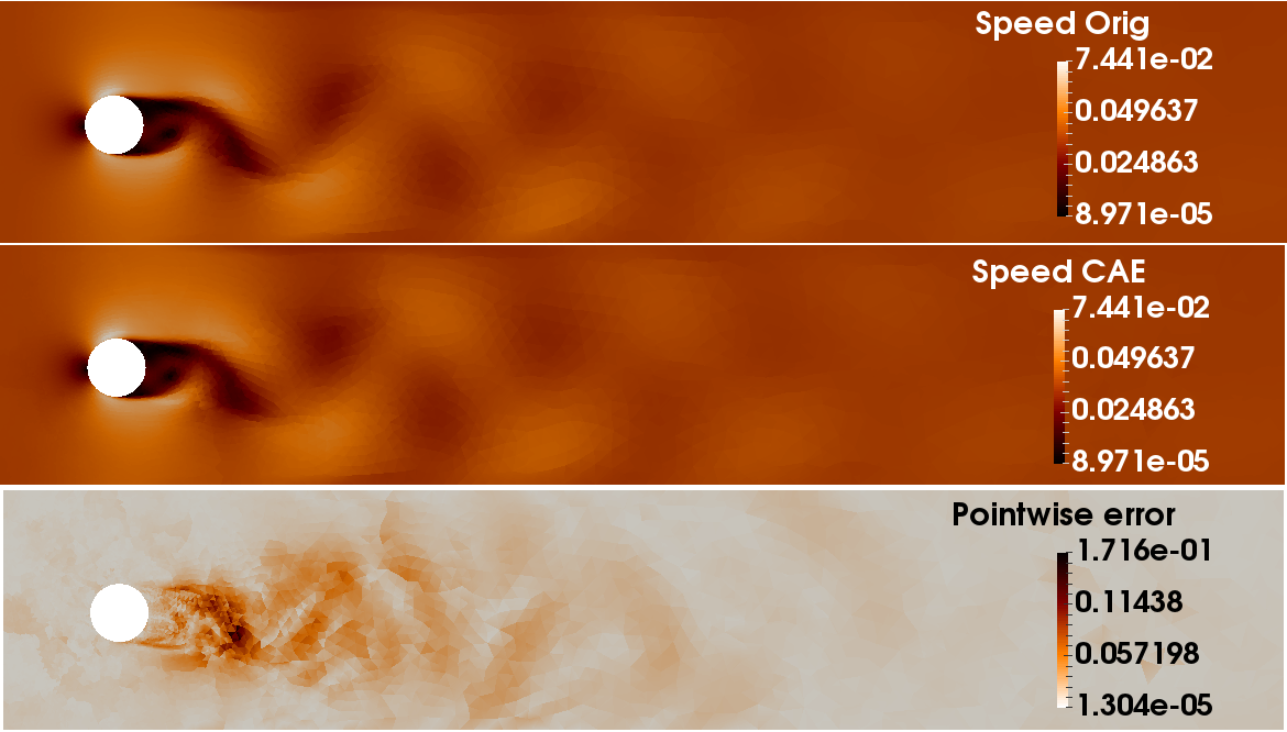
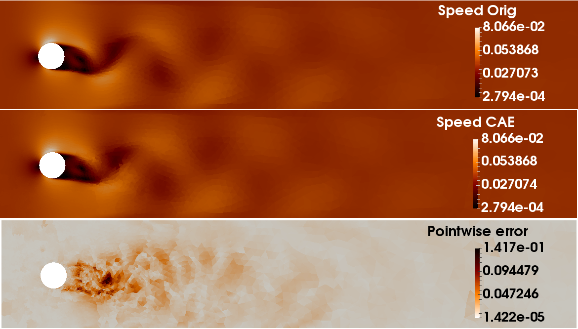
4.4.3 Performance of the autoencoder based on two SFCs with nearest-neighbour smoothing for different compression ratios
For the convolutional autoencoder based on two space-filling curves with nearest-neighbour smoothing (CAE-2SFC-NN), the effect of dimension of latent space is explored. In the previous section, a dimension of 128 was used. Here, the autoencoder is trained multiple times for 64, 32, 16, 8, 4, 2 and 1 latent variables. After 2000 epochs (4000 in the case of 2 and 1 variables), the losses are shown in Figure 15 and Table 17, which indicate that, even though we reduce the number of compressed variables, the accuracy is still reasonable. In fact, the spatial distribution of the results for compression to 1 variable looks similar to the spatial distribution for 128 compressed variables in Figure 14. Notice that as the number of compressed variables is reduced the gap between the validation and training loss is reduced. This could be interpreted as a reduction in the tendency for over-fitting as the number of latent or compressed variables is reduced. Also notice from Figures 15 and 16 that the greater the number of compressed variables the shorter the wavelength of the structures in the error fields. Thus, with smaller compression sizes one seems to be able to capture the basic structures and as more variables are introduced finer scale structures are captured. Note that the imprints of the space-filling curves are not noticeable for the smaller number of compressed variables, therefore, the nearest-neighbour smoothing layers of the autoencoder must be performing well. However, one can see this imprint in the error field for larger numbers of compressed variables.
Comparing the CAE-2SFC-NN network with the SVD (see Table 17), we find that for compressed variable sizes of 128, 64, 32, 16, and 8, the truncation error of the SVD is smaller than the loss of the autoencoders. However, for compressed variables sizes of 4, 2 and 1, the losses of the autoencoders are smaller than those of the SVD. This is because flow past a cylinder is a smooth problem, periodic in time, for which only a few SVD modes are needed to accurately represent the flow. However, this is still a hard problem for the an autoencoder, and the CAE-2SFC-NN network does manage to more effectively compress to a small number of variables than the SVD approach.
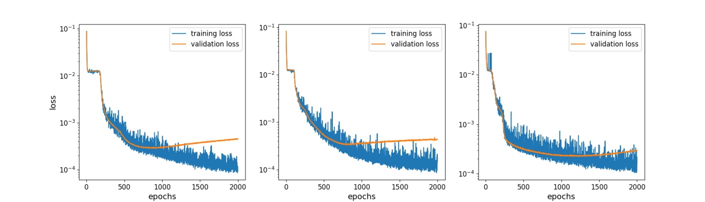
| number of compressed variables | ||||||||
|---|---|---|---|---|---|---|---|---|
| 128 | 64 | 32 | 16 | 8 | 4 | 2 | 1 | |
| Training data | ||||||||
| Validation data | ||||||||
| Test data | ||||||||
| SVD | ||||||||
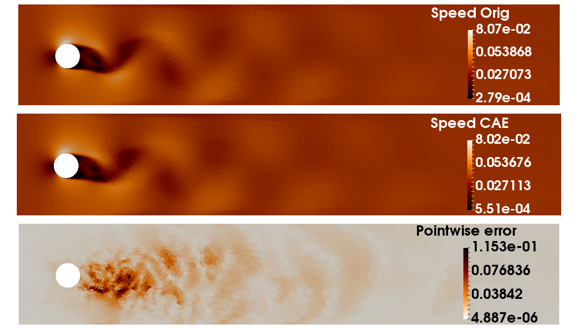
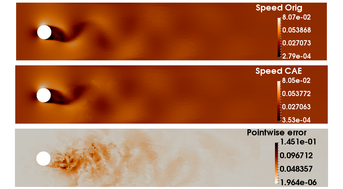
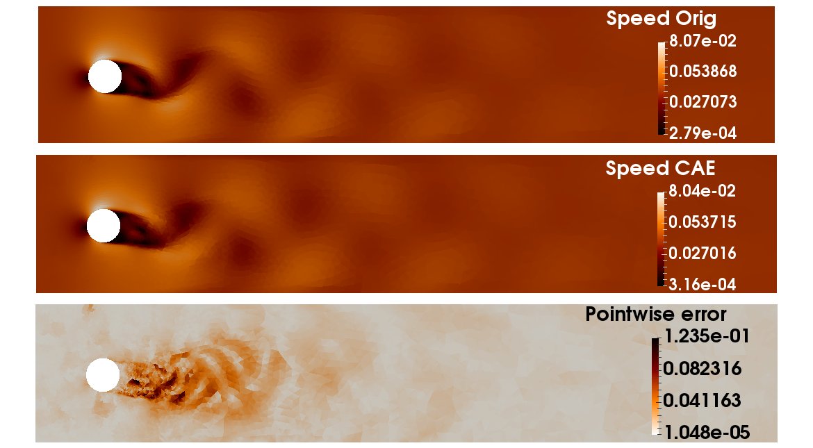
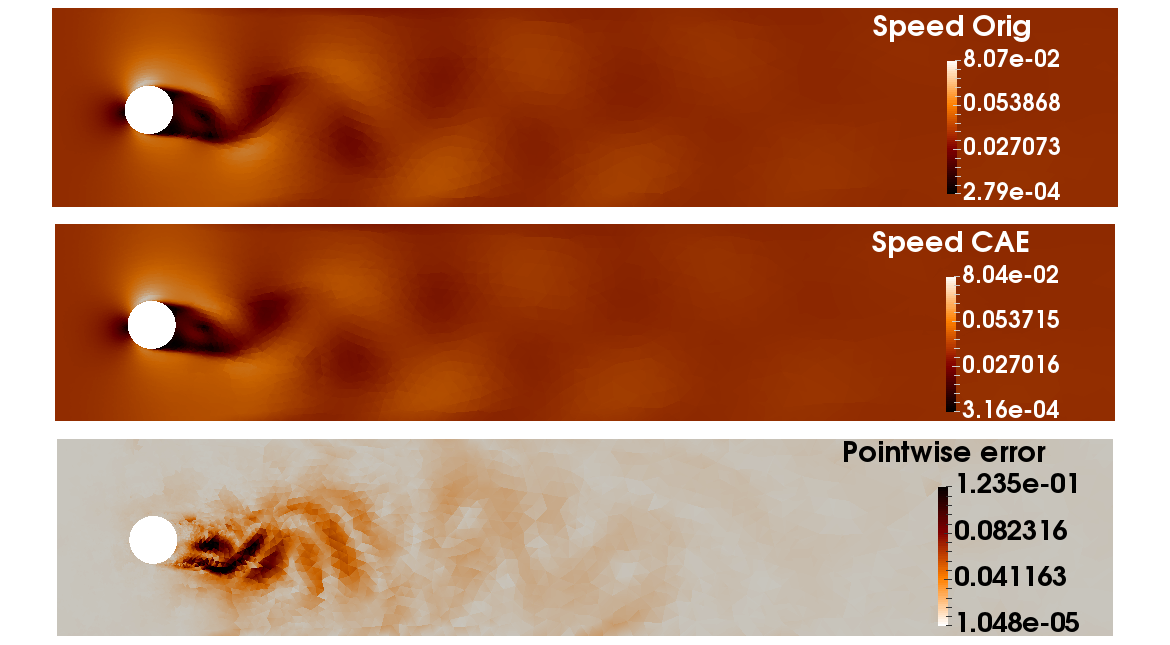
Finally, a box and whisker plot can be seen in Figure 17. Here, the average absolute error in space is calculated for each example in the data sets for each compression ratio. Then, for each compression ratio and for each data set (training, validation, test), the median error is shown in orange, the upper (Q3) and lower (Q1) quartiles are represented by the box and the whiskers indicate the range of the data, taken as the data points closest to Q1-1.5IQR and Q3+1.5IQR, where the inter-quartile range (IQR) is Q3-Q1. Approximately 1% of the data points are considered to be outliers and are not shown. The variation over training (left), validation (centre) and test (right) data is similar due to the time-periodic problem studied here. Remarkably, as the number of latent variables is reduced, the range of errors becomes slightly larger, but there is no obvious upward trend. This agrees with the plots shown in Figure 16, where the accuracy seems not to be affected by the number of latent variables.
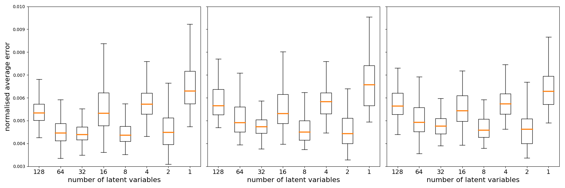
5 Future work
The SFC-based approach to applying CNNs to data on unstructured meshes has been established in this paper. Furthermore, this approach has been applied to data on an unstructured mesh with differing areas of resolution. A next big challenge will be to apply the SFC-based CNN approach to solutions on adaptive meshes, that is meshes that change their topology and resolution as time evolves in order to optimally represent the physics. The SFC-based approach has the potential to be able to deal with even this, as the filters do not necessarily depended on the mesh. One may, for example, be able to take into account the connectivity by also including the coordinates as inputs to the 1D CNNs or to the SFC-based CNN. Once these issues are dealt with then it may be possible to apply (at least as a starting model for training) the weights from one example problem to the weights of a different fluids problem. In addition, the approach may be used to interpolate from one mesh to a different mesh while increasing the numerical resolution and sharpness of the features especially when interpolating onto meshes or mesh parts that have finer resolution than the original mesh. This interpolation approach is very much akin to the deblurring GAN-CNN or DeblurGAN [49].
Further work will also be needed to explore the application of the method to 3D, with, potentially, the use of three space-filling curves.
Another area of further study is the inclusion of the time dimension within the CNN. Rather than treating the time dimension independently [50], a space-filling curve could be applied simultaneously to four-dimensional solutions (three spatial dimensions and one temporal dimension).
6 Conclusions
The space-filling curve (SFC) approach shows great promise in enabling the application of convolutional networks to data from unstructured meshes. The approach has several features that make it ideal for application to convolutional neural networks (CNNs). This includes the aptitude of SFCs for automatic coarsening of meshes.
We demonstrate the approach by compressing the results of solutions of the Navier-Stokes equations for incompressible flow past a cylinder and show that it is able to compress of the order of 50,000 solution variables with a complex discontinuous Galerkin stencil down to between 128 variables and 1 variable, while maintaining accuracy. We also show that it can be beneficial to use two space-filling curves to help increase the accuracy of the CNN. We also found it important to reduce the noise in the outputs of the SFC-based autoencoders by introducing sparse smoothing layers near the output (and input) of the autoencoders. On structured mesh data sets the accuracy of the new SFC-based autoencoders are similar to classical autoencoders and it seems worth exploring their comparative capabilities even for data on structured grids.
Acknowledgements
The authors would like to acknowledge the following EPSRC grants: MUFFINS (EP/P033180/1); PREMIERE (EP/T000414/1); MAGIC (EP/N010221/1) and INHALE (EP/T003189/1).
References
- [1] D. Minnen, J. Ballé, G. Toderici, High-Fidelity Generative Image Compression, arXiV: 1809.02736 (2018).
- [2] F. Mentzer, G. Toderici, M. Tschannen, E. Agustsson, High-Fidelity Generative Image Compression, arXiV: 2006.09965v2 (2020).
- [3] A. Krizhevsky, I. Sutskever, G. E. Hinton, ImageNet Classification with Deep Convolutional Neural Networks, in: F. Pereira, C. J. C. Burges, L. Bottou, K. Q. Weinberger (Eds.), Advances in Neural Information Processing Systems 25, Curran Associates, Inc., 2012, pp. 1097–1105.
- [4] J. Yim, J. Ju, H. Jung, J. Kim, Image classification using convolutional neural networks with multi-stage feature, in: J.-H. Kim, W. Yang, J. Jo, P. Sincak, H. Myung (Eds.), Robot Intelligence Technology and Applications 3, Springer International Publishing, Cham, 2015, pp. 587–594.
- [5] F. J. Gonzalez, M. Balajewicz, Deep convolutional recurrent autoencoders for learning low-dimensional feature dynamics of fluid systems, arXiV: 1808.01346 (2018).
- [6] K. Lee, K. T. Carlberg, Model reduction of dynamical systems on nonlinear manifolds using deep convolutional autoencoders, Journal of Computational Physics 404 (2020) 108973.
- [7] S. Walton, O. Hassan, K. Morgan, Advances in co-volume mesh generation and mesh optimisation techniques, Computers & Structures 181 (2017) 70–88.
- [8] Z. Xie, D. Pavlidis, P. Salinas, J. R. Percival, C. C. Pain, O. K. Matar, A balanced-force control volume finite element method for interfacial flows with surface tension using adaptive anisotropic unstructured meshes, Computers & Fluids 138 (2016) 38–50.
- [9] A. E. Kampitsis, A. Adam, P. Salinas, C. C. Pain, A. H. Muggeridge, M. D. Jackson, Dynamic adaptive mesh optimisation for immiscible viscous fingering, Computational Geosciences 24 (2020) 1221–1237.
- [10] F. Alauzet, A. Loseille, A Decade of Progress on Anisotropic Mesh Adaptation for Computational Fluid Dynamics, Computer-Aided Design 72 (2016) 13–39.
- [11] J. Mack, R. Arcucci, M. Molina-Solana, Y.-K. Guo, Attention-based Convolutional Autoencoders for 3D-Variational Data Assimilation, Computer Methods in Applied Mechanics and Engineering 372 (2020) 113291.
- [12] K. Lee, K. T. Carlberg, Model reduction of dynamical systems on nonlinear manifolds using deep convolutional autoencoders, Journal of Computational Physics 404 (2020) 108973.
- [13] J. Xu, K. Duraisamy, Multi-level convolutional autoencoder networks for parametric prediction of spatio-temporal dynamics, Computer Methods in Applied Mechanics and Engineering 372 (2020) 113379.
- [14] Z. Wu, S. Pan, F. Chen, G. Long, C. Zhang, P. Yu, A Comprehensive Survey on Graph Neural Networks, IEEE Transactions on Neural Networks and Learning Systems (2020) 1–21.
- [15] T. N. Kipf, M. Welling, Semi-Supervised Classification with Graph Convolutional Networks, arXiV: 1609.02907 (2017).
- [16] A. Paszke, S. Gross, F. Massa, A. Lerer, J. Bradbury, G. Chanan, T. Killeen, Z. Lin, N. Gimelshein, L. Antiga, A. Desmaison, A. Kopf, E. Yang, Z. DeVito, M. Raison, A. Tejani, S. Chilamkurthy, B. Steiner, L. Fang, J. Bai, S. Chintala, PyTorch: An Imperative Style, High-Performance Deep Learning Library, in: H. Wallach, H. Larochelle, A. Beygelzimer, F. d'Alché-Buc, E. Fox, R. Garnett (Eds.), Advances in Neural Information Processing Systems 32, Curran Associates, Inc., 2019, pp. 8024–8035.
- [17] R. Hanocka, A. Hertz, N. Fish, R. Giryes, S. Fleishman, D. Cohen-Or, MeshCNN: A Network with an Edge, ACM Trans. Graph. 38 (4) (2019).
- [18] S. Dargaville, A. G. Buchan, R. P. Smedley-Stevenson, P. N. Smith, C. C. Pain, A comparison of element agglomeration algorithms for unstructured geometric multigrid, arXiV: 2005.09104 (2020).
- [19] Q. Lu, C. Chen, W. Xie, Y. Luo, PointNGCNN: Deep convolutional networks on 3D point clouds with neighborhood graph filters, Computers & Graphics 86 (2020) 42–51.
- [20] C. C. Pain, A. P. Umpleby, C. R. E. de Oliveira, A. J. H. Goddard, Tetrahedral mesh optimisation and adaptivity for steady-state and transient finite element calculations, Computer Methods in Applied Mechanics and Engineering 190 (29) (2001) 3771–3796.
- [21] A. Sanchez-Gonzalez, J. Godwin, T. Pfaff, R. Ying, J. Leskovec, P. W. Battaglia, Learning to Simulate Complex Physics with Graph Networks, arXiV: 2002.09405v2 (2020).
- [22] T. Pfaff, M. Fortunato, A. Sanchez-Gonzalez, P. W. Battaglia, Learning Mesh-Based Simulation with Graph Networks, arXiV: 2010.03409 (2020).
- [23] G. Peano, Sur une courbe, qui remplit toute une aire plane, Mathematische Annalen (in French) 36 (1890) 157–160.
- [24] D. Hilbert, Ueber die stetige abbildung einer line auf ein flächenstück, Mathematische Annalen 38 (1891) 459–460.
- [25] H. Sagan, Space-Filling Curves, Springer, 1994.
- [26] M. Bader, Space-Filling Curves: An Introduction with Applications in Scientific Computing, Springer, 2013.
- [27] C. Böhm, M. Perdacher, C. Plant, A Novel Hilbert Curve for Cache-locality Preserving Loops, IEEE Transactions on Big Data (2018) 1–15.
- [28] H.-J. Bungartz, M. Mehl, T. Weinzierl, A parallel adaptive cartesian pde solver using space–filling curves, in: W. Nagel, W. Walter, W. Lehner (Eds.), Euro-Par 2006 Parallel Processing, Springer Berlin Heidelberg, Berlin, Heidelberg, 2006, pp. 1064–1074.
- [29] J. Behrens, J. Zimmermann, Parallelizing an unstructured grid generator with a space-filling curve approach, in: A. Bode, T. Ludwig, W. Karl, R. Wismüller (Eds.), Euro-Par 2000 Parallel Processing, Springer Berlin Heidelberg, Berlin, Heidelberg, 2000, pp. 815–823.
- [30] D. A. Sprecher, S. Draghici, Space-filling curves and Kolmogorov superposition-based neural networks, Neural Networks 15 (2002) 57–67.
- [31] N. Papamarkos, Color Reduction Using Local Features and a Kohonen Self-Organized Feature Map Neural Network, International Journal of Imaging Systems and Technology 10 (1999) 404–409.
- [32] M. M. Anjum, I. A. Tahmid, M. S. Rahman, CNN Model With Hilbert Curve Representation of DNA Sequence For Enhancer Prediction, bioRxiv: 10.1101/552141 (2019).
- [33] B. Yin, M. Balvert, D. Zambrano, A. Schönhuth, S. M. Bohte, An Image Representation Based Convolutional Network for DNA Classification, 6th International Conference on Learning Representations (2018).
- [34] E. Skubalska-Rafajłowicz, Applications of the space-filling curves with data driven measure-preserving property, Nonlinear Analysis: Theory, Methods & Applications 30 (3) (1997) 1305–1310.
- [35] T. Corcoran, R. Zamora-Resendiz, X. Liu, S. Crivelli, A Spatial Mapping Algorithm with Applications in Deep Learning-Based Structure Classification, arXiv: 1802.02532v2 (2018).
- [36] T. Phillips, C. E. Heaney, P. N. Smith, C. C. Pain, An autoencoder-based reduced-order model for eigenvalue problems with application to neutron diffusion problems, arXiv:2008.10532 [math.NA], (2020).
- [37] G. E. Hinton, A. Krizhevsky, S. Wang, Transforming Auto-encoders, in: T. Honkela, W. Duch, M. Girolami, S. Kaski (Eds.), Artificial Neural Networks and Machine Learning – ICANN 2011, Springer, 2011, pp. 44–51.
- [38] J. Hesthaven, S. Ubbiali, Non-intrusive reduced order modeling of nonlinear problems using neural networks, Journal of Computational Physics 363 (2018) 55–78.
- [39] D. Xiao, C. E. Heaney, L. Mottet, F. Fang, W. Lin, I. M. Navon, Y. Guo, O. K. Matar, A. G. Robins, C. C. Pain, A reduced order model for turbulent flows in the urban environment using machine learning, Building and Environment 148 (2019) 323–337.
- [40] D. Xiao, C. Heaney, F. Fang, L. Mottet, R. Hu, D. Bistrian, E. Aristodemou, I. Navon, C. Pain, A domain decomposition non-intrusive reduced order model for turbulent flows, Computers & Fluids 182 (2019) 15–27.
- [41] S. E. Ahmed, S. M. Rahman, O. San, A. Rasheed, I. M. Navon, Memory embedded non-intrusive reduced order modeling of non-ergodic flows, Physics of Fluids 31 (12) (2019) 126602.
- [42] A. Buluç, H. Meyerhenke, I. Safro, P. Sanders, C. Schulz, Recent Advances in Graph Partitioning, Springer International Publishing, 2016, pp. 117–158.
- [43] A. P. Fitzgerald, B. Kochunas, S. Stimpson, T. Downar, Spatial decomposition of structured grids for nuclear reactor simulations, Annals of Nuclear Energy 132 (2019) 686–701.
- [44] T. Kawamoto, M. Tsubaki, T. Obuchi, Mean-field theory of graph neural networks in graph partitioning, Journal of Statistical Mechanics: Theory and Experiment 12 (2019) 124007.
- [45] G. Karypis, V. Kumar, Multilevel -way Partitioning Scheme for Irregular Graphs, J. Parallel Distrib. Comput. 48 (1) (1998) 96–129.
- [46] G. Karypis, V. Kumar, A Fast and High Quality Multilevel Scheme for Partitioning Irregular Graphs, SIAM J. Sci. Comput. 20 (1) (1998) 359–392.
- [47] I. Moulitsas, G. Karypis, Multilevel algorithms for generating coarse grids for multigrid methods, in: SC ’01: Proceedings of the 2001 ACM/IEEE Conference on Supercomputing, 2001, pp. 15–15.
- [48] C. C. Pain, C. R. E. De Oliveira, A. J. H. Goddard, A neural network graph partitioning procedure for grid-based domain decomposition, International Journal for Numerical Methods in Engineering 44 (5) (1999) 593–613.
- [49] O. Kupyn, V. Budzan, M. Mykhailych, D. Mishkin, J. Matas, DeblurGAN: Blind Motion Deblurring Using Conditional Adversarial Networks, in: 2018 IEEE/CVF Conference on Computer Vision and Pattern Recognition, 2018, pp. 8183–8192.
- [50] P. Wu, J. Sun, X. Chang, W. Zhang, R. Arcucci, Y. Guo, C. C. Pain, Data-driven reduced order model with temporal convolutional neural network, Computer Methods in Applied Mechanics and Engineering 360 (2020) 360–373.