Variational Discrete Action Theory

Abstract

Here we propose the Variational Discrete Action Theory (VDAT) to study the ground state properties of quantum many-body Hamiltonians. VDAT is a variational theory based on the sequential product density matrix (SPD) ansatz, characterized by an integer $\mathcal{N}$, which monotonically approaches the exact solution with increasing $\mathcal{N}$. To evaluate the SPD, we introduce a discrete action and a corresponding integer time Green’s function. We use VDAT to exactly evaluate the SPD in two canonical models of interacting electrons: the Anderson impurity model (AIM) and the $d=\infty$ Hubbard model. For the latter, we evaluate $\mathcal{N}=2-4$, where $\mathcal{N}=2$ recovers the Gutzwiller approximation (GA), and we show that $\mathcal{N}=3$, which exactly evaluates the Gutzwiller-Baeriswyl wave function, provides a truly minimal yet precise description of Mott physics with a cost similar to the GA. VDAT is a flexible theory for studying quantum Hamiltonians, competing both with state-of-the-art methods and simple, efficient approaches all within a single framework.

Computing the ground state properties of quantum many-body Hamiltonians is a fundamental task in physics. A common strategy to approximately solve a Hamiltonian is the use of variational wave functions, which allows one to find the best solution within some fraction of the Hilbert space. A generic approach is to start from some reference wave function and apply some projector, as in the well known JastrowJastrow (1955) and GutzwillerGutzwiller (1963, 1964, 1965) variational wave functions. A key limitation to such approaches is that they often cannot be intelligently improved, meaning that it is difficult to increase the searchable region of Hilbert space efficiently. One approach to address this limitation is tensor network methodsMcculloch (2007); Schollwock (2005, 2011), where some control parameter increases accuracy at some computational cost; but these approaches have only proven well suited for low dimensional systems.

Here we propose a new class of variational density matrices: the sequential product density matrix (SPD). The SPD is motivated by the Trotter-SuzukiSuzuki (1993) decomposition, and is characterized by an integer $\mathcal{N}$. The SPD provides a paradigm for variational approaches in that the precision can be systematically improved by increasing $\mathcal{N}$, and it can be applied beyond low dimensions. In practice, such an ansatz is not useful unless one has a systematic and efficient approach for evaluating it. Our key development is the introduction of the discrete action theory (DAT) and the corresponding integer time Green’s function, which may be used for evaluating an SPD. The DAT has a perfect parallel to the standard many-body Green’s function formalism, though with non-trivial differences; such as a new discrete Dyson equation. Many of the key ideas from traditional many-body theory can immediately be generalized to the DAT, such as the Dynamical Mean-Field Theory (DMFT)Georges et al. (1996). Using the DAT for evaluating the SPD, we can then perform the variational minimization to obtain the ground state, and we refer to this entire approach as the Variational Discrete Action Theory (VDAT). There is companion manuscript to this paper which provides extensive derivations and minimal examples to document the foundations of VDATCheng and Marianetti (2020a).

Given a Hamiltonian $\hat{H}=\hat{H}_{0}+\hat{V}$, where $\hat{H}_{0}$ is non-interacting and $\hat{V}$ is interacting, we motivate the SPD by considering the following variational wave function:

$$\exp(\gamma_{1}\hat{H}_{0})\exp(g_{1}\hat{V})...\exp(\gamma_{N}\hat{H}_{0})\exp(g_{N}\hat{V})|\varphi_{0}\rangle,$$ (1)

where $\gamma_{i},g_{i}$ are variational parameters and $|\varphi_{0}\rangle$ is the ground state wave function of $\hat{H}_{0}$. Equation 1 can be viewed as a variational application of the Trotter-Suzuki decompositionTrotter (1959); Suzuki (1976, 1993), where the $N\rightarrow\infty$ limit will cover the exact ground state wave function. The essence of this ansatz was first proposed several decades ago by Dzierzawa et. al Dzierzawa et al. (1995), motivated by the generalization of the Baeriswyl wave functionBaeriswyl (1987, 2000) by OtsukaOtsuka (1992); and all of this work was motivated by improving upon the well known Gutzwiller wave functionGutzwiller (1963). More recently, a unitary version of this wave function was proposed in the context of quantum computing by Farhi et. alFarhi et al. (2014), and further extended by Wecker et. al Wecker et al. (2015) and Grimsley et. alGrimsley et al. (2019). Our SPD further generalizes the idea behind Eq. 1.

Given a Hamiltonian with $L$ spin orbitals, the SPD is given as

$$\hat{\varrho}=\exp\left(\bm{\gamma}_{1}\cdot\hat{\bm{n}}\right)\hat{P}_{1}\dots\exp\left(\bm{\gamma}_{\mathcal{N}}\cdot\hat{\bm{n}}\right)\hat{P}_{\mathcal{N}}=\hat{\mathcal{P}}_{1}\dots\hat{\mathcal{P}}_{\mathcal{N}},$$ (2)

where $\hat{P}_{\tau}$ is a generic interacting projector, and $\tau=1,\dots,\mathcal{N}$ is the integer time label; $\exp\left(\bm{\gamma}_{\tau}\cdot\hat{\bm{n}}\right)$ is the noninteracting projector, where $\bm{\gamma}_{\tau}\cdot\hat{\bm{n}}\equiv\sum_{i=1}^{L}\sum_{j=1}^{L}[\bm{\gamma}_{\tau}]_{ij}[\hat{\bm{n}}]_{ij}$ and $[\hat{\bm{n}}]_{ij}=\hat{a}_{i}^{\dagger}\hat{a}_{j}$; and $\hat{\mathcal{P}}_{\tau}=\exp\left(\bm{\gamma}_{\tau}\cdot\hat{\bm{n}}\right)\hat{P}_{\tau}$. When using the SPD as a variational density matrix, it must be restricted to a symmetric and semi-definite form; and there are two variants for a given $\mathcal{N}$Cheng and Marianetti (2020a). Referring to $\tau$ as an integer time is likely counterintuitive, but this will prove essential in building the DAT formalism to evaluate the SPD. It should be noted that the most general non-interacting projector would include the terms $\hat{a}_{i}^{\dagger}\hat{a}_{j}^{\dagger}$ and $\hat{a}_{i}\hat{a}_{j}$, but we presently omit them for brevity. We also define a non-interacting SPD as $\hat{\varrho}_{0}=\exp\left(\bm{\gamma}_{1}\cdot\hat{\bm{n}}\right)\dots\exp\left(\bm{\gamma}_{\mathcal{N}}\cdot\hat{\bm{n}}\right)$, which will be the starting point for the perturbative expansion of the SPD. The variational parameters of the SPD are the $\bm{\gamma}_{\tau}$ and the parameters within $\hat{P}_{\tau}$. A common choice for the interacting projector is $\hat{P}_{\tau}=\exp(\hat{\mathcal{V}}_{\tau})=\exp\left(\sum_{i}g_{\tau,i}\hat{V}_{i}\right)$ where $\sum_{i}\hat{V}_{i}=\hat{V}$ is some decomposition of the interacting portion of the Hamiltonian, though there are many possible choices (e.g. as in the Jastrow wave function for the Hubbard modelJastrow (1955); Fazekas and Penc (1988); Yokoyama and Shiba (1990); Capello et al. (2005)). The SPD brings several generalizations over Eq. 1. First and most obviously, the SPD explicitly includes all possible variational freedom at the single particle level, and formally allows for a generic interacting projector. Second, and less obviously, the SPD form allows for a systematic evaluation using the integer time Green’s function formalism introduced in this paper. It is useful to note that $\mathcal{N}=1$ recovers the well known Hartree-Fock approximation; $\mathcal{N}=2$ recovers the Gutzwiller, Baeriswyl, and Jastrow wave functions, in addition to unitary and variational coupled clusterBartlett and Noga (1988); Bartlett et al. (1989); Kutzelnigg (1991); Taube and Bartlett (2006); and $\mathcal{N}=3$ recovers the Gutzwiller-BaeriswylOtsuka (1992) and Baeriswyl-GutzwillerDzierzawa et al. (1995) wave functions (see Cheng and Marianetti (2020a) for a detailed discussion).

We now introduce the DAT to evaluate the Hamiltonian under the SPD at a given set of variational parameters. We begin with the integer time Green’s function formalism, where the integer time evolution in the integer time interaction representation is given as

$$\hat{O}_{I}\left(\tau\right)=\hat{U}_{I}(\tau)\hat{O}\hat{U}_{I}(\tau)^{-1},$$ (3)

$$\hat{U}_{I}(\tau)=\exp\left(\bm{\gamma}_{1}\cdot\hat{\bm{n}}\right)\dots\exp\left(\bm{\gamma}_{\tau}\cdot\hat{\bm{n}}\right),$$ (4)

where $\tau=1,\dots,\mathcal{N}$. Taylor series expanding the interacting projector, the expectation value of some operator $\hat{O}$ under the SPD is given as

$$\langle\hat{O}\rangle_{\hat{\varrho}} =\frac{\sum_{n=0}^{\infty}\frac{1}{n!}\langle\textrm{T}(\sum_{\tau=1}^{\mathcal{N}}\hat{\mathcal{V}}_{\tau,I}(\tau))^{n}\hat{O}_{I}(\mathcal{N})\rangle_{\hat{\varrho}_{0}}}{\sum_{n=0}^{\infty}\frac{1}{n!}\langle\textrm{T}(\sum_{\tau=1}^{\mathcal{N}}\hat{\mathcal{V}}_{\tau,I}(\tau))^{n}\rangle_{\hat{\varrho}_{0}}},$$ (5)

where the quantum average is defined as $\langle\hat{O}\rangle_{\hat{\rho}}=\textrm{Tr}(\hat{\rho}\hat{O})/\textrm{Tr}(\hat{\rho})$; the integer time ordering operator T first sorts the operators according to ascending integer time and then according to the position in the original ordering of operators and finally the result is presented from left to right; additionally, the resulting sign must be tracked when permuting operators. It should be noted that our time convention is opposite to the usual definitionMahan (2000). Each term in Eq. 5 can be evaluated via the non-interacting integer time Green’s function

$$[\boldsymbol{g}_{0}]_{k\tau,k^{\prime}\tau^{\prime}}=\langle\text{T}\hat{a}_{k,I}^{\dagger}\left(\tau\right)a_{k^{\prime},I}\left(\tau^{\prime}\right)\rangle_{\hat{\varrho}_{0}},$$ (6)

using the integer time Wick’s theoremCheng and Marianetti (2020a). In general, Eq. 5 will require the evaluation of an infinite number of terms, but if the interacting projector is restricted to a local subspace, we can resum the expansion into a finite number of terms.

For a test case, we consider the Anderson impurity model (AIM) on a ringCheng and Marianetti (2020a), which has recently been extensively studied using density matrix renormalization group (DMRG)Barcza et al. (2019). In this case, the interacting projectors can be chosen as local to the impurity, and the exponential can be rewritten as a sum of Hubbard operators within the impurity as

$$\hat{P}_{\tau} =\exp(\mu_{\tau}\sum_{\sigma}\hat{n}_{\sigma}+u_{\tau}\hat{n}_{\uparrow}\hat{n}_{\downarrow})=\sum_{\Gamma}P_{\tau,\Gamma}\hat{X}_{\Gamma},$$ (7)

where $\hat{X}_{\Gamma}=|\Gamma\rangle\langle\Gamma|$ is a Hubbard operator and $P_{\tau,0}=1$, $P_{\tau,\sigma}=\exp(\mu_{\tau})$, and $P_{\tau,2}=\exp(2\mu_{\tau}+u_{\tau})$; and the subscripts $0,\sigma,2$ correspond to empty, singly occupied, and double occupied local states, respectively. For this interacting projector, Eq. 5 will have a finite number of terms and thus can be evaluated exactly.

The computational cost of evaluating the total energy for a given SPD in the AIM is dictated by two factors. The first cost is associated with constructing the non-interacting integer time Green’s function for the entire system, which scales at worst as $\mathcal{N}L^{3}$. Second, there is the cost of evaluating the total energy using the integer time Wick’s theorem, which scales exponentially with the number of integer time steps $\mathcal{N}$Cheng and Marianetti (2020a). For the particular cases of $\mathcal{N}\leq 3$ and $L\approx 1000$, the computational cost is always dominated by $L$ via the first factor, and therefore in this scenario a single evaluation of VDAT has a minimal computational cost, given that the limitation is the diagonalization of the non-interacting Hamiltonian.

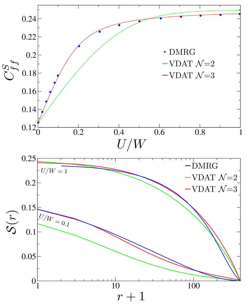
Figure 1: A comparison of VDAT and published DMRG resultsBarcza et al. (2019) for the Anderson impurity model on a ring with $L=1397$. (Panel a) A plot of $C_{ff}^{S}=\langle S_{f}^{z}S_{f}^{z}\rangle=\frac{1}{4}\langle(\hat{n}_{f\uparrow}-\hat{n}_{f\downarrow})^{2}\rangle$ vs. $U/W$. (Panel b) The unscreened spin $\mathcal{S}(r)$ vs. the distance from the impurity site.

Having all the machinery necessary to evaluate the total energy under the SPD, we can then minimize over the variational parameters in order to determine the ground state of the Hamiltonian. Given the specific parameterization of the SPD we have chosen (see reference Cheng and Marianetti (2020a), Section VII B 1), there will be $\lceil(\mathcal{N}-1)/2\rceil$ interacting variational parameters, while there will be $3\lfloor(\mathcal{N}-1)/2\rfloor$ non-interacting variational parameters. Therefore, the total number of iterations for minimizing the energy under the SPD will be a constant that is independent of $L$, and VDAT for $1<\mathcal{N}\leq 3$ should have a similar cost to $\mathcal{N}=1$ (i.e. Hartree-Fock).

We now evaluate the local spin correlation $C_{ff}^{S}=\langle S_{f}^{z}S_{f}^{z}\rangle=\frac{1}{4}\langle(\hat{n}_{f\uparrow}-\hat{n}_{f\downarrow})^{2}\rangle$, which probes the double occupancy on the impurity site (see Figure 1, panel $a$), and compare to numerically exact DMRG calculationsBarcza et al. (2019). For $\mathcal{N}=2$, which recovers the Gutzwiller wave function, the result is only a rough approximation to the DMRG results. Alternatively, $\mathcal{N}=3$ only shows very small deviations from the DMRG results. Clearly, the SPD converges extremely rapidly with respect to $\mathcal{N}$. What is especially remarkable is that $\mathcal{N}=3$ has a computational cost similar to Hartree-Fock, yet has a precision approaching DMRG. We can also compute the unscreened spin (see Figure 1, panel $b$), which is a far more challenging observable given that it involves a long range correlation between the impurity and the bathBarcza et al. (2019). Once again, $\mathcal{N}=2$ has reasonable but relatively inaccurate results, while $\mathcal{N}=3$ is quantitatively accurate.

The preceding approach of using the integer time Wick’s theorem to sum all diagrams would be intractable for a general interacting system. This motivates us to push forward our discrete action theory, and generalize the traditional tools of many-body physics. Consider the interacting integer time Green’s function under an SPD defined as

$$[\boldsymbol{g}]_{k\tau,k^{\prime}\tau^{\prime}} =\langle\text{T}\hat{a}_{k}^{\dagger}\left(\tau\right)\hat{a}_{k^{\prime}}\left(\tau^{\prime}\right)\rangle_{\hat{\varrho}},$$ (8)

where $\tau=1,\dots,\mathcal{N}$ and $k=1,\dots,L$ and $\hat{O}(\tau)$ is an operator in the integer time Heisenberg representation defined as

$$\hat{O}(\tau) =\hat{U}_{\tau}\hat{O}\hat{U}_{\tau}^{-1}, \hat{U}_{\tau}=\hat{\mathcal{P}}_{1}\dots\hat{\mathcal{P}}_{\tau}.$$ (9)

Furthermore, when constructing interaction energies and computing the gradient of the total energy with respect to the variational parameters, we will need general integer time correlation functions $\langle\textrm{T}\hat{O}_{1}(\tau_{1})...\hat{O}_{M}(\tau_{M})\rangle_{\hat{\varrho}}$; which can be rewritten in the integer time Schrodinger representation as

$$\frac{\langle\textrm{T}\hat{\mathcal{A}}\hat{O}_{1,S}(\tau_{1})...\hat{O}_{M,S}(\tau_{M})\rangle_{\hat{1}}}{\langle\textrm{T}\hat{\mathcal{A}}\rangle_{\hat{1}}},\hskip 10.00002pt\textrm{where}\hskip 10.00002pt\hat{\mathcal{A}}=\hat{\mathcal{A}}_{0}\hat{P},$$ (10)

$$\hat{\mathcal{A}}_{0}=\exp\big{(}\sum_{\tau=1}^{\mathcal{N}}\bm{\gamma}_{\tau}\cdot\hat{\bm{n}}_{S}(\tau)\big{)},\hskip 10.00002pt\hat{P}=\prod_{\tau=1}^{\mathcal{N}}\hat{P}_{\tau,S}(\tau),$$ (11)

and $\hat{O}_{S}(\tau)$ is an operator in the integer time Schrodinger representation where $\hat{O}_{S}(\tau)=\hat{O}$ after applying the time ordering operator. We refer to $\hat{\mathcal{A}}$ as the discrete action, given that it encodes all possible integer time correlations under the SPD. Moreover, we can generalize the form of $\hat{\mathcal{A}}$ such that it can describe integer time correlations beyond the SPD, and an important generalization allows for an $\hat{\mathcal{A}}_{0}$ which has off-diagonal integer time components as

$$\hat{\mathcal{A}}_{0}=\exp(\sum_{k\tau k^{\prime}\tau^{\prime}}[\boldsymbol{v}]_{k\tau,k^{\prime}\tau^{\prime}}\hat{a}_{k,S}^{\dagger}(\tau)\hat{a}_{k^{\prime},S}(\tau^{\prime})),$$ (12)

where $\boldsymbol{v}$ is a general matrix of dimension $L\mathcal{N}\times L\mathcal{N}$Cheng and Marianetti (2020a). We refer to this more general form as a canonical discrete action (CDA), which will be critical to exactly evaluating the SPD in $d=\infty$.

It is useful to define the discrete generating function, which encodes all information of the discrete action into a scalar function

$$Z(\boldsymbol{g}_{0})\equiv\langle\hat{\mathcal{A}}\rangle_{\hat{1}}/\langle\hat{\mathcal{A}}_{0}\rangle_{\hat{1}}.$$ (13)

For example, using the discrete generating function and the Lie group properties of the non-interacting many-body density matrix, we can derive the discrete Dyson equation

$$(\bm{g}^{-1}-\boldsymbol{1})=(\bm{g}_{0}^{-1}-\boldsymbol{1})\exp(-\boldsymbol{\Sigma})^{T},$$ (14)

where the integer time self-energy $\bm{\Sigma}$ and exponential integer time self-energy $\boldsymbol{S}$ are obtained from the generating function as

$$\exp\left(\bm{\Sigma}\right)^{T}=\boldsymbol{S}^{-1}=\boldsymbol{1}+\frac{\boldsymbol{1}}{Z\boldsymbol{1}-\frac{\partial Z}{\partial\boldsymbol{g}_{0}^{T}}\boldsymbol{g}_{0}}\frac{\partial Z}{\partial\boldsymbol{g}_{0}^{T}}.$$ (15)

This discrete Dyson equation plays a central role in our formalism, much like the traditional Dyson equation. In the limit of large $\mathcal{N}$, the discrete Dyson equation reverts to the usual Dyson equation assuming that the SPD is chosen as the Trotter-Suzuki decompositionCheng and Marianetti (2020a). While we have illustrated the single particle integer time Green’s function above, any n-particle integer time correlation function can be determined from the generating functionCheng and Marianetti (2020a).

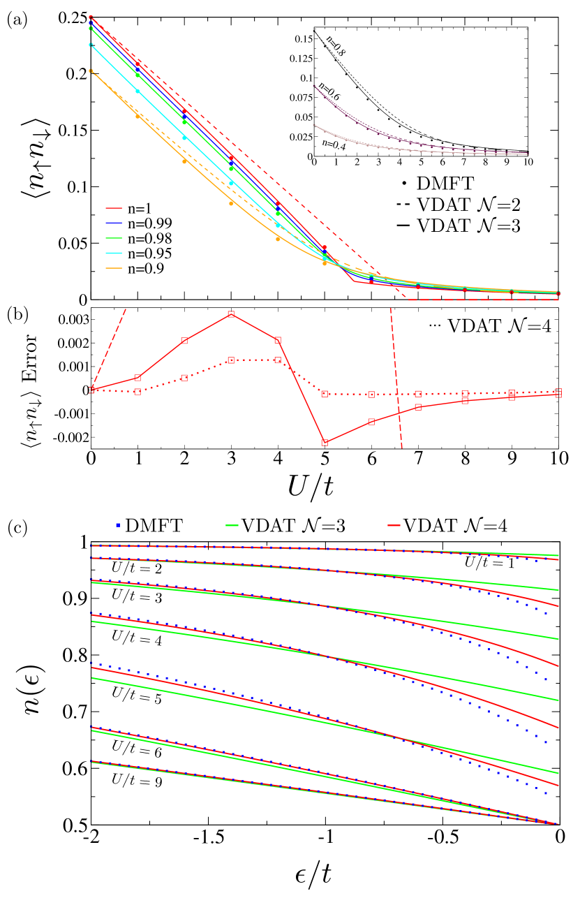
Figure 2: Results for the $d=\infty$ Hubbard model on the Bethe lattice. (Panel $a$) The double occupancy vs. $U/W$ for VDAT($\mathcal{N}=3$) (lines) and DMFT (points). Densities of 1, 0.99, 0.98, 0.95, and 0.9 are evaluated. (Inset) Densities of 0.8, 0.6, and 0.4 are evaluated. (Panel $b$) The difference in the double occupancy between VDAT($\mathcal{N}=2-4$) and DMFT vs. $U/W$. (Panel $c$) The density distribution vs. energy for various values of $U/t$ evaluated using VDAT($\mathcal{N}=3,4$) and DMFT.

Having completed the discrete action theory formalism, we now have the proper tools to study the single-band Hubbard model, and we use an SPD with an interacting projector $\hat{P}_{\tau}=\exp(\mu_{\tau}\sum_{i\sigma}\hat{n}_{i\sigma}+\sum_{i}u_{\tau}\hat{n}_{i\uparrow}\hat{n}_{i\downarrow})$, while the non-interacting projector uses uses a diagonal $\boldsymbol{\gamma}_{\tau}$ in the basis that diagonalizes the non-interacting Hamiltonian. In order to evaluate the discrete generating function, we introduce the self-consistent canonical discrete action approximation (SCDA), which is the integer time analogue of DMFTGeorges et al. (1996). The SCDA maps the SPD to a collection of CDA’s, with one CDA corresponding to each site in the lattice, and the non-interacting part of the CDA is determined self-consistently while the interacting part is taken from the SPD. The essence of the SCDA is the assumption that the integer time self-energy is local

$$\bm{\Sigma}_{ij}\left(\bm{g}\right)=\delta_{ij}\bm{\Sigma}_{loc}\left(\bm{g}_{loc}\right).$$ (16)

Analogous to DMFT, which assumes a local self-energy and becomes exact in $d=\infty$, the SCDA exactly evaluates the SPD in $d=\infty$. For example, the SCDA for $\mathcal{N}=2$ recovers the result that the Gutzwiller approximation exactly evaluates the Gutzwiller wave function in $d=\infty$Metzner and Vollhardt (1988). Additionally, the SCDA for $\mathcal{N}=3$ exactly evaluates generalizations of the Gutzwiller-Baeriswyl and Baeriswyl-Gutzwiller wave functions in $d=\infty$, which had not yet been achieved. For $\mathcal{N}>3$, the SCDA exactly evaluates an infinite number of variational wave functions in $d=\infty$ that have not yet been considered.

The SCDA algorithm exactly parallels the DMFT algorithm. We can begin with a guess for the non-interacting integer time Green’s function $\bm{\mathcal{G}}=\int d\epsilon D\left(\epsilon\right)\bm{g}_{0}\left(\epsilon\right)$ for the CDA. We can then compute the generating function of the CDA, which yields $\bm{S}_{loc}$. We then use this exponential integer time self-energy to update the interacting integer time Green’s function for each energy orbital as

$$\bm{g}\left(\epsilon\right)=\frac{\boldsymbol{1}}{\boldsymbol{g}_{0}\left(\epsilon\right)+\left(\boldsymbol{1}-\bm{g}_{0}\left(\epsilon\right)\right)\bm{S}_{loc}}\bm{g}_{0}\left(\epsilon\right).$$ (17)

Then we obtain the new interacting local integer time Green’s function as $\bm{g}_{loc}=\int d\epsilon D\left(\epsilon\right)\bm{g}\left(\epsilon\right)$. Finally, the new non-interacting integer time Green’s function of the CDA is

$$\bm{\mathcal{G}}=\bm{S}_{loc}\frac{\boldsymbol{1}}{\boldsymbol{1}+\bm{g}_{loc}\left(\bm{S}_{loc}-\boldsymbol{1}\right)}\bm{g}{}_{loc}.$$ (18)

This procedure must be iterated until self-consistency is achieved, which yields a single evaluation of the SPD for a given set of variational parameters. The above procedure is applicable to any Hubbard-like model, but it will yield an exact evaluation of the SPD for infinite dimensionsCheng and Marianetti (2020a).

The number of variational parameters for the interacting projector will be the same as the AIM, while for the non-interacting projector we restrict to five variational parameters for each integer timeCheng and Marianetti (2020a). The main computational complexity of solving the Hubbard model as compared to the AIM is that we must perform a self-consistency condition, though this can normally be achieved in small number of iterations. We now address the $d=\infty$ Hubbard model on the Bethe lattice. It should be emphasized that the computed ground state energy within VDAT is a rigorous upper bound for the exact ground state energy, and we can compare to the numerically exact dynamical mean-field theory results obtained using the numerical renormalization group (NRG) method as the impurity solverZitko and Pruschke (2009). We examine the double occupancy as a function of $U/t$, where we present VDAT results for $\mathcal{N}=3$ and selected results for $\mathcal{N}=2$, where the latter is the well known Gutzwiller approximation (see Figure 2, panel $a$). For half-filling, shown in red, we see that VDAT $\mathcal{N}=3$ is very close to the DMFT solutions (points), reliably capturing the Mott metal-insulator transition, and illustrating drastic improvement beyond $\mathcal{N}=2$. Furthermore, we can see that VDAT clearly captures the sensitive changes with small doping, illustrated for the densities of 1, 0.99, 0.98, 0.95, and 0.9. We can also proceed to much larger dopings (see inset), where VDAT once again reliably describes the DMFT solution. All VDAT results discussed thus far have been for $\mathcal{N}\leq 3$, and it is interesting to consider $\mathcal{N}=4$ to better understand the convergence of the VDAT. Therefore, we examine the error in the double occupancy at half filling for $\mathcal{N}=2-4$ (see Figure 2, panel $b$). We see that $\mathcal{N}=4$ has a smaller error for all values of $U/t$, as it must, and the error for large $U/t$ is nearly zero. Another interesting quantity is the density distribution (see Figure 2, panel $c$), which is more challenging given that only the average enters the total energy. It is well know that $\mathcal{N}=2$ (i.e. Gutzwiller) produces a constant density distribution, and we show that $\mathcal{N}>2$ produces a non-trivial energy dependence. This quantity converges less rapidly than the double occupancy, presumably because it does not directly enter the Hamiltonian.

In conclusion, we have proven that VDAT with $\mathcal{N}=3$ already yields efficient and precise results for the Anderson Impurity model and for the $d=\infty$ Hubbard model. Furthermore, it is straightforward to address the multi-orbital Hubbard modelCheng and Marianetti (2020a), which is under way. Given that VDAT recovers the Hartree-Fock and Gutzwiller wave functions, it is clear that VDAT can be combined with DFT in the same spirit as DFT+UAnisimov et al. (1997) and DFT+GutzwillerDeng et al. (2009); and DFT+VDAT would be a prime candidate as an efficient first-principles approach to strongly correlated materials, which should rival DFT+DMFTKotliar et al. (2006).

Additionally, there are many possible directions for future development, given the obvious parallels between the discrete action theory and traditional many-body Green’s function theory. Both diagrammatic and auxiliary field quantum Monte-Carlo could be generalized to our formalism. While our present work on the SPD has used real variational parameters, we can apply VDAT using an SPD with unitary projectorsCheng and Marianetti (2020a), which could have utility in quantum computingFarhi et al. (2014); Wecker et al. (2015); Grimsley et al. (2019) and unitary coupled cluster theoryBartlett et al. (1989); Taube and Bartlett (2006); Kutzelnigg (1991). Finally, VDAT will be a key tool for parameterizing energy functionals in the context of the off-shell effective energy theoryCheng and Marianetti (2020b), which can be viewed as a formally exact construction based on an $\mathcal{N}=2$ SPD.

This work was supported by the grant DE-SC0016507 funded by the U.S. Department of Energy, Office of Science. This research used resources of the National Energy Research Scientific Computing Center, a DOE Office of Science User Facility supported by the Office of Science of the U.S. Department of Energy under Contract No. DE-AC02-05CH11231.

References

- Jastrow (1955) R. Jastrow, Phys. Rev. 98, 1479 (1955).
- Gutzwiller (1963) M. C. Gutzwiller, Phys. Rev. Lett. 10, 159 (1963).
- Gutzwiller (1964) M. C. Gutzwiller, Physical Review 134, 923 (1964).
- Gutzwiller (1965) M. C. Gutzwiller, Physical Review 137, 1726 (1965).
- Mcculloch (2007) I. P. Mcculloch, Journal Of Statistical Mechanics-theory And Experiment 10, 10014 (2007).
- Schollwock (2005) U. Schollwock, Rev. Mod. Phys. 77, 259 (2005).
- Schollwock (2011) U. Schollwock, Annals Of Physics 326, 96 (2011).
- Suzuki (1993) M. Suzuki, Physica A-statistical Mechanics And Its Applications 194, 432 (1993).
- Georges et al. (1996) A. Georges, G. Kotliar, W. Krauth, and M. J. Rozenberg, Rev. Mod. Phys. 68, 13 (1996).
- Cheng and Marianetti (2020a) Z. Cheng and C. A. Marianetti, Phys. Rev. B [jointly submitted with current manuscript] 0, 0 (2020a).
- Trotter (1959) H. F. Trotter, Proceedings of the American Mathematical Society 10, 545 (1959).
- Suzuki (1976) M. Suzuki, Communications In Mathematical Physics 51, 183 (1976).
- Dzierzawa et al. (1995) M. Dzierzawa, D. Baeriswyl, and M. Distasio, Phys. Rev. B 51, 1993 (1995).
- Baeriswyl (1987) D. Baeriswyl, in Nonlinearity in Condensed Matter, edited by A. R. Bishop, D. K. Campbell, and S. E. Trullinger (Springer-Verlag, Berlin, 1987) 1st ed., pp. 183–193.
- Baeriswyl (2000) D. Baeriswyl, Foundations Of Physics 30, 2033 (2000).
- Otsuka (1992) H. Otsuka, J. Phys. Soc. Jpn. 61, 1645 (1992).
- Farhi et al. (2014) E. Farhi, J. Goldstone, and S. Gutmann, arXiv:1411.4028 (2014).
- Wecker et al. (2015) D. Wecker, M. B. Hastings, and M. Troyer, Physical Review A 92, 042303 (2015).
- Grimsley et al. (2019) H. R. Grimsley, S. E. Economou, E. Barnes, and N. J. Mayhall, Nature Communications 10, 3007 (2019).
- Fazekas and Penc (1988) P. Fazekas and K. Penc, International Journal of Modern Physics B 2, 1021 (1988).
- Yokoyama and Shiba (1990) H. Yokoyama and H. Shiba, J. Phys. Soc. Jpn. 59, 3669 (1990).
- Capello et al. (2005) M. Capello, F. Becca, M. Fabrizio, S. Sorella, and E. Tosatti, Phys. Rev. Lett. 94, 026406 (2005).
- Bartlett and Noga (1988) R. J. Bartlett and J. Noga, Chemical Physics Letters 150, 29 (1988).
- Bartlett et al. (1989) R. J. Bartlett, S. A. Kucharski, and J. Noga, Chemical Physics Letters 155, 133 (1989).
- Kutzelnigg (1991) W. Kutzelnigg, Theoretica Chimica Acta 80, 349 (1991).
- Taube and Bartlett (2006) A. G. Taube and R. J. Bartlett, International Journal Of Quantum Chemistry 106, 3393 (2006).
- Mahan (2000) G. D. Mahan, Many-Particle Physics (Physics of Solids and Liquids) (Springer, 2000).
- Barcza et al. (2019) G. Barcza, F. Gebhard, T. Linneweber, and O. Legeza, Phys. Rev. B 99, 165130 (2019).
- Metzner and Vollhardt (1988) W. Metzner and D. Vollhardt, Phys. Rev. B 37, 7382 (1988).
- Zitko and Pruschke (2009) R. Zitko and T. Pruschke, Phys. Rev. B 79, 085106 (2009).
- Anisimov et al. (1997) V. I. Anisimov, F. Aryasetiawan, and A. I. Lichtenstein, Journal Of Physics-condensed Matter 9, 767 (1997).
- Deng et al. (2009) X. Y. Deng, L. Wang, X. Dai, and Z. Fang, Phys. Rev. B 79, 075114 (2009).
- Kotliar et al. (2006) G. Kotliar, S. Y. Savrasov, K. Haule, V. S. Oudovenko, O. Parcollet, and C. A. Marianetti, Rev. Mod. Phys. 78, 865 (2006).
- Cheng and Marianetti (2020b) Z. Cheng and C. A. Marianetti, Phys. Rev. B 101, 081105 (2020b).