Foundations of the Variational Discrete Action Theory

Abstract

Variational wave functions and Green’s functions are two important paradigms for solving quantum Hamiltonians, each having their own advantages. Here we detail the Variational Discrete Action Theory (VDAT), which exploits the advantages of both paradigms in order to approximately solve the ground state of quantum Hamiltonians. VDAT consists of two central components: the sequential product density matrix (SPD) ansatz and a discrete action associated with the SPD. The SPD is a variational ansatz inspired by the Trotter decomposition and characterized by an integer $\mathcal{N}$, recovering many well known variational wave functions, in addition to the exact solution for $\mathcal{N}=\infty$. The discrete action describes all dynamical information of an effective integer time evolution with respect to the SPD. We generalize the path integral to our integer time formalism, which converts a dynamic correlation function in integer time to a static correlation function in a compound space. We also generalize the usual many-body Green’s function formalism to integer time, which results in analogous but distinct mathematical structures, yielding integer time versions of the generating functional, Dyson equation, and Bethe-Salpeter equation. We prove that the SPD can be exactly evaluated in the multi-band Anderson impurity model (AIM) by summing a finite number of diagrams. For the multi-band Hubbard model, we prove that the self-consistent canonical discrete action approximation (SCDA), which is the integer time analogue of the dynamical mean-field theory, exactly evaluates the SPD for d=$\infty$. VDAT within the SCDA provides an efficient yet reliable method for capturing the local physics of quantum lattice models, which will have broad applications for strongly correlated electron materials. More generally, VDAT should find applications in various many-body problems in physics.

I Introduction

The quantum many-body problem represents a forefront in most areas of physics, and determining the ground state of the Hamiltonian is a primary objective. Variational wave functions are a key paradigm for solving the ground state of a Hamiltonian. Simple variational approaches such as the Hartree-Fock approximation provide a baseline for understanding many-body systems at a modest computational cost. There are many more sophisticated variational wave functions, such as the Jastrow wave function[1, 2] or unitary coupled cluster[3, 4, 5], but most approaches do not have a natural mechanism for trading off between accuracy and computational cost, which will be a key idea addressed in this paper.

Another viewpoint for addressing the many-body problem is to start from the formally exact density matrix and perform the Trotter-Suzuki decomposition[6, 7, 8], yielding the Euclidean path integral, which may then be approximately evaluated using quantum Monte-Carlo or using a diagrammatic approach. A prominent example of the former is auxiliary field quantum Monte-Carlo (AFQMC)[9, 10], which requires a relatively fine discretization of imaginary time in order to achieve converged ground state properties. If one is only seeking ground state properties, no dynamical information needs to be extracted from the Green’s function, which motivates the possibility of obtaining highly precise ground state properties from an extremely coarse discretization of imaginary time. This suggestion can be realized by creating a variational density matrix ansatz based upon the Trotter-Suzuki decomposition, and in this paper we propose the sequential product density matrix (SPD). Given that the SPD is inspired by the Trotter-Suzuki decomposition, it is naturally characterized by an integer $\mathcal{N}$, which controls the trade-off between accuracy and computational complexity.

The SPD is an extremely generic ansatz which can recover a large number of well known variational wave functions. An example at $\mathcal{N}=1$ is the Hartree-Fock approximation, while examples at $\mathcal{N}=2$ include the Gutzwiller wave function[11, 12, 13] and the Jastrow wave function[1, 2] (see Subsection II.4 for a complete list). Therefore, we already begin with decades of intuition for the efficacy of this ansatz at small $\mathcal{N}$, and one can easily envision the potency of larger $\mathcal{N}$. Many formal constructions are useful for organizing ideas, but the question is whether or not they can be evaluated in practice. A key development in this paper is demonstrating that our proposed integer time Green’s function and its corresponding discrete action theory provide a rich formalism for systematically evaluating observables under the SPD ansatz. Most practically, this yields new theories that have not yet been discovered and can be implemented in practice. More generally, this discrete action theory provides a new way to think about variational wave functions in the context of Green’s function. The discrete action theory naturally gives rise to its own version of the path integral, generating functional, Dyson equation, and Bethe-Salpeter equation. Therefore, many of the key ideas from Green’s functions may be generalized to the discrete action theory. The discrete action theory can then be used along with the variational principle to give rise to the variational discrete action theory (VDAT). Furthermore, the discrete action theory provides many different avenues for precisely evaluating the SPD at a given set of variational parameters.

A decisive milestone of this paper is proving that a certain type of SPD can be exactly evaluated in infinite dimensions, implying that we can achieve a strict upper bound on the ground state energy in this case. This result extends the well known fact that the Gutzwiller wave function is exactly evaluated by the Gutzwiller approximation for the Hubbard model in $d=\infty$[14, 15, 16, 17], proving that the Gutwziller-Baeriswyl[18] and Baeriswyl-Gutzwiller[19] wave functions can be exactly evaluated in $d=\infty$, in addition to an infinite number of more precise generalizations. As a result, VDAT is a potent theory for efficiently and precisely evaluating the Hubbard model in $d=\infty$. Indeed, we have demonstrated that VDAT achieves highly precise results in the $d=\infty$ Hubbard model for $\mathcal{N}=3$[20]. The VDAT method can immediately be understood as a practically important tool given our knowledge of the dynamical mean-field theory (DMFT)[21, 22, 23], which allows for the numerically exact solution of the Hubbard model in infinite dimensions. DMFT is the de facto standard for capturing local physics in models of strongly correlated electrons, and plays a key role in describing realistic strongly correlated materials in the context of DFT+DMFT[24]. Given that VDAT precisely captures the physics of infinite dimensions at a tiny fraction of the cost of DMFT, VDAT might be transformational as an efficient replacement for DMFT in the context of ground state properties. A DFT+VDAT theory might finally yield a first-principles approach of strongly correlated electron materials with a computational overhead not far beyond DFT itself, yet contain all of the physics of DFT+DMFT, and more.

In this study, we restrict ourselves to static observables at zero temperature. Given that VDAT is a variational theory with an explicit density matrix ansatz, one can also naturally study static observables at finite temperatures, though doing so requires the direct evaluation of the entropy of the SPD. Evaluating the entropy is highly nontrivial, even in the relatively simple case of $\mathcal{N}=2$ or the Gutzwiller wave function[25, 26, 27]. Therefore, extending the VDAT formalism to finite temperatures will be pursued in future work. Another important direction for VDAT would be to study excited states, which are not naturally captured in a variational theory. However, one can straightforwardly apply the Landau-Gutzwiller quasiparticle approach[28], which would clearly result in a Fermi liquid picture which can go beyond Gutzwiller. More generally, there is a possibility that the incoherent part of the spectrum may be recovered with further extensions given that VDAT with $\mathcal{N}>2$ precisely captures the insulating phase in the single-band Hubbard model[20].

The structure of this manuscript is as follows. In Section II, we begin by motivating and introducing a generic SPD, and introduce three important classes of SPD which are useful for prominent models of interacting electrons. Additionally, we apply the SPD to the Hubbard plaquette, where it can be exactly evaluated, to illustrate the convergence of the SPD with respect to $\mathcal{N}$. In Section III, we introduce the notion of the integer correlation function, and demonstrate how it can be evaluated using the integer time Wick’s theorem. A pedagogical example is given for the Anderson impurity model containing a single bath site. In Section IV, we introduce the notion of a discrete action, and generalize the standard tools of many-body physics to the integer time case, including the integer time path integral, the discrete generating function, the discrete Dyson equation, and the discrete Bethe-Salpeter equation. In Section V, we introduce the canonical discrete action, and use it to evaluate the SPD that is associated with the Anderson impurity model. In Section VI, we introduce the self-consistent canonical discrete action approximation (SCDA), and we prove that it exactly evaluates the SPD-d in infinite dimensions. Furthermore, in the case of $\mathcal{N}=2$ we pedagogically illustrate how the SCDA recovers the Gutzwiller approximation, and we derive basis-independent, rotationally invariant Gutzwiller equations for the multi-band Hubbard model. In Section VII, we discuss the general workflow of performing a VDAT calculation. Finally, we provide an appendix which illustrates the Lie group properties of the non-interacting density matrix (see Subsection X.1), in addition to a second appendix which proves the integer time Wick’s theorem (see Subsection X.2). Additionally, we provide supplementary information which illustrates the evaluation of the CDA for the case of a single orbital and $\mathcal{N}=3$[29]. It should be noted that there is short companion manuscript for this paper, which highlights the basic aspects of the VDAT while presenting key results on the Anderson impurity model and the $d=\infty$ Hubbard model[20].

II Sequential Product Density Matrix (SPD)

II.1 Motivating the SPD

Here we motivate the notion of the sequential product density matrix (SPD), which is the variational ansatz for the VDAT. First, let us begin by recalling the variational principle at zero temperature. Given some Hamiltonian $\hat{H}$, the ground state energy is obtained by the constrained search over the density matrix ansatz as

$$\mathcal{E}=\min_{\hat{\rho}}\left\{\langle\hat{H}\rangle_{\hat{\rho}}|\hat{\rho}\in\mathcal{C}\right\},$$ (1)

where $\mathcal{C}$ denotes the space of all density matrices described by the ansatz, and we used the notation $\langle\hat{O}\rangle_{\hat{\rho}}=\textrm{Tr}(\hat{\rho}\hat{O})/\textrm{Tr}(\hat{\rho})$ for the measurement of some operator $\hat{O}$ under a density matrix $\hat{\rho}$.

We now consider a special case of the SPD ansatz which is dictated by the form of the Hamiltonian, and we refer to this ansatz as the Trotter SPD. The essence of the wave function version of the Trotter SPD was anticipated several decades ago[19]. To motivate the Trotter SPD, consider the Trotter-Suzuki Decomposition[6, 7, 8] of a finite temperature density matrix for a system with $L$ spin orbitals

$$\exp(-\beta\hat{H}) \approx\prod_{\tau=1}^{\mathcal{N}}\exp(-\frac{\beta}{\mathcal{N}}\hat{H}_{0})\exp(-\frac{\beta}{\mathcal{N}}\hat{V}),$$ (2)

where $\hat{H}=\hat{H}_{0}+\hat{V}$ is the Hamiltonian, $\hat{H}_{0}$ is the non-interacting part, and $\hat{V}$ is interacting part. The Trotter SPD ansatz can be obtained by replacing $-\beta/\mathcal{N}$ with variational parameters $\gamma_{\tau},g_{\tau}$ with $\tau=1\dots\mathcal{N}$ as

$$\hat{\varrho}=\exp(\gamma_{1}\hat{H}_{0})\exp(g_{1}\hat{V})\dots\exp(\gamma_{\mathcal{N}}\hat{H}_{0})\exp(g_{\mathcal{N}}\hat{V}).$$ (3)

We see that the Trotter SPD is composed of pairs of non-interacting and interacting projectors, which are sequentially multiplied together. Considering the case of $\mathcal{N}=2$

$$\hat{\varrho}=\exp(\gamma_{1}\hat{H}_{0})\exp(g_{1}\hat{V})\exp(\gamma_{2}\hat{H}_{0})\exp(g_{2}\hat{V}),$$ (4)

where we can restrict to a purely Hermitian form (see Section II.2 for a detailed discussion) as

$$\hat{\varrho}=\exp(g_{1}\hat{V})\exp(\gamma_{1}\hat{H}_{0})\exp(g_{1}^{*}\hat{V}).$$ (5)

In the limit of large $\mathcal{N}$ and $\beta$, the variational theorem can select $\gamma_{\tau}=g_{\tau}=-\beta/\mathcal{N}$ and recover the exact density matrix. For a given finite $\mathcal{N}$, the variational principle will gaurantee that the Trotter SPD will generate superior ground state results to any approach based on the standard Trotter-Suzuki decomposition, such as auxiliary field quantum Monte-Carlo (AFQMC)[9, 10, 30, 31].

To understand the convergence of the Trotter SPD with $\mathcal{N}$, it is useful to solve the Hubbard plaquette, which is the one dimensional Hubbard model with four sites and translational symmetry, at half-filling and zero temperature; where we can directly evaluate the exact solution. We restrict our attention to the case of real variational parameters (see Subsection II.3 for a general discussion). The Hubbard model is given by $\hat{H}_{0}=t\sum_{\langle ij\rangle\sigma}\hat{a}_{i\sigma}^{\dagger}\hat{a}_{j\sigma}$ and $\hat{V}=U\sum_{i}\hat{n}_{i\uparrow}\hat{n}_{i\downarrow}$, where $\langle ij\rangle$ denotes nearest neighbor sites. We now compare the double occupancy, $\langle\hat{n}_{i\uparrow}\hat{n}_{i\downarrow}\rangle=\partial\langle\hat{H}\rangle/\partial U$, of the exact solution and Trotter SPD ansatz at a given $\mathcal{N}$ (see Figure 1, panel $a$). For $\mathcal{N}=2$, which rigorously recovers the Gutzwiller wave function[11, 12, 13], there is relatively large disagreement with the exact solution, completely missing the discontinuity at $U/t=0$. Moving to $\mathcal{N}=3$, we recover the discontinuity, and move closer to the exact solution. For $\mathcal{N}=11$, there is almost no discernible difference with the exact solution, and we see that the error monotonically decreases with increasing $\mathcal{N}$. Similarly, the error for the total energy monotonically decreases with increasing $\mathcal{N}$, as it must (see Figure 1, panel $b$). This simple example illustrates the efficacy of the Trotter SPD ansatz[32]. However, it should be emphasized that one can only directly evaluate an SPD in the full Fock space for a sufficiently small system. For macroscopic systems in the thermodynamic limit, we will need a more advanced approach (see Sections III and IV).

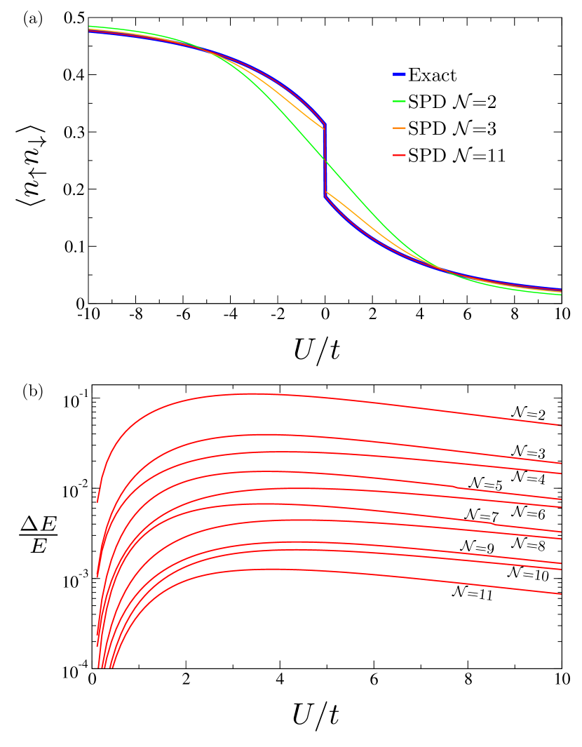
Figure 1: Results for the Hubbard Plaquette, comparing the Trotter SPD ansatz to the exact solution. (Panel a) Double occupancy vs. $U/t$ for $\mathcal{N}=$ 2, 3, and 11. (Panel b) Energy error vs. $U/t$ for $\mathcal{N}=$ 2-11.

II.2 Defining the SPD

The Trotter SPD defined in the preceding subsection is dictated based on the form of the Hamiltonian being studied, whereas a general SPD will not have such limitations. In general, one can enlarge both the non-interacting and interacting projectors to include operators which do not appear in the Hamiltonian itself, in addition to changing the relative weights of existing operators. For the non-interacting projector, we replace $\exp(\gamma_{\tau}\hat{H}_{0})$ from the Trotter SPD with $\exp\left(\bm{\gamma}_{\tau}\cdot\hat{\bm{n}}\right)$, where

$$\bm{\gamma}_{\tau}\cdot\hat{\bm{n}} \equiv\sum_{i=1}^{L}\sum_{j=1}^{L}[\bm{\gamma}_{\tau}]_{ij}[\hat{\bm{n}}]_{ij}, [\hat{\bm{n}}]_{ij}=\hat{a}_{i}^{\dagger}\hat{a}_{j},$$ (6)

where $[\bm{\gamma}_{\tau}]_{ij}$ are the variational parameters and $L$ is the number of spin orbitals. It should be noted that most general non-interacting projector would include the terms $\hat{a}_{i}^{\dagger}\hat{a}_{j}^{\dagger}$ and $\hat{a}_{i}\hat{a}_{j}$, but we presently omit them for brevity. For the interacting projector, we replace $\exp(g_{1}\hat{V})$ with $\hat{P}_{\tau}$, which is a general Bosonic interacting projector which will have various constraints (see Subsection II.3). Mathematically, the general SPD is then defined as

$$\hat{\varrho}=\exp\left(\bm{\gamma}_{1}\cdot\hat{\bm{n}}\right)\hat{P}_{1}\dots\exp\left(\bm{\gamma}_{\mathcal{N}}\cdot\hat{\bm{n}}\right)\hat{P}_{\mathcal{N}}=\hat{\mathcal{P}}_{1}\dots\hat{\mathcal{P}}_{\mathcal{N}},$$ (7)

$$\hat{\mathcal{P}}_{\tau}=\exp\left(\bm{\gamma}_{\tau}\cdot\hat{\bm{n}}\right)\hat{P}_{\tau},$$ (8)

$$\hat{P}_{\tau}=\exp(\hat{\mathcal{V}}_{\tau})=\sum_{\Gamma\Gamma^{\prime}}P_{\tau,\Gamma\Gamma^{\prime}}\hat{X}_{\Gamma\Gamma^{\prime}},$$ (9)

where $\Gamma,\Gamma^{\prime}$ label the basis of the Fock space, $\hat{X}_{\Gamma\Gamma^{\prime}}$ is a Hubbard operator, and $P_{\tau,\Gamma\Gamma^{\prime}}$ are the variational parameters. The SPD will always be constrained to be Hermitian and semi-definite, and this can be achieved in two distinct ways, which we denote as Gutzwiller-type (G-type) or Baeriswyl-type (B-type). For $\mathcal{N}=1,2,3$, the G-type and B-type SPD are

$$\hat{\varrho}_{G}^{\left(1\right)}= \exp( \bm{\gamma}_{1}\cdot\hat{\bm{n}}),$$ (10)

$$\hat{\varrho}_{G}^{\left(2\right)}= \hat{P}_{1}\exp( \bm{\gamma}_{2}\cdot\hat{\bm{n}})\hat{P}_{1}^{\dagger},$$ (11)

$$\hat{\varrho}_{G}^{\left(3\right)}= \exp\left(\bm{\gamma}_{1}\cdot\hat{\bm{n}}\right)\hat{P}_{1}\exp( \bm{\gamma}_{2}\cdot\hat{\bm{n}})\hat{P}_{1}^{\dagger}\exp(\bm{\gamma}_{1}^{\dagger}\cdot\hat{\bm{n}}),$$ (12)

$$\hat{\varrho}_{B}^{\left(1\right)}= \hat{P}_{1},$$ (13)

$$\hat{\varrho}_{B}^{\left(2\right)}= \exp\left(\bm{\gamma}_{1}\cdot\hat{\bm{n}}\right) \hat{P}_{1}\exp(\bm{\gamma}_{1}^{\dagger}\cdot\hat{\bm{n}}),$$ (14)

$$\hat{\varrho}_{B}^{\left(3\right)}= \hat{P}_{1}\exp\left(\bm{\gamma}_{2}\cdot\hat{\bm{n}}\right) \hat{P}_{2}\exp(\bm{\gamma}_{2}^{\dagger}\cdot\hat{\bm{n}})\hat{P}_{1}^{\dagger}.$$ (15)

For $\mathcal{N}=1$ and G-type, $\bm{\gamma}_{1}$ is a Hermitian matrix. For $\mathcal{N}=2,3$ and G-type, $\bm{\gamma}_{2}$ is a Hermitian matrix, while $\bm{\gamma}_{1}$ and $\hat{P}_{1}$ are unrestricted. For $\mathcal{N}=1,2$ and B-type, $\hat{P_{1}}$ is a Hermitian and semi-definite operator, while $\bm{\gamma}_{1}$ is unrestricted. For $\mathcal{N}=3$ and B-type, $\hat{P_{2}}$ is a Hermitian and semi-definite operator, while $\bm{\gamma}_{2}$ and $\hat{P_{1}}$ are unrestricted. It should be noted that the $\mathcal{N}+1$ G-type can always recover the $\mathcal{N}$ B-type, and vice versa. Throughout the manuscript, we will use the G-type unless otherwise specified.

It should be noted that the G-type and B-type ansatz are related by an abstract “dual” transformation, whereby one ansatz can be obtained from the other by interchanging the interacting projector with the non-interacting projector. This same notion of a dual transformation has been previously introduced in the context of the Gutzwiller, Baeriswyl, Gutzwiller-Baeriswyl, and Baeriswyl-Gutzwiller wave functions[19], in addition to the $\mathcal{K}$ and $\mathcal{X}$ formulations of the off-shell effective energy theory[33].

II.3 Classification of the SPD

The generically defined Hermitian and semi-definite SPD encompasses a broad variety of possibilities, and it is useful to consider various categorization schemes. The first categorization we consider is partitioning into projective, unitary, or general SPD. A projective SPD is the subset where the unrestricted projectors are Hermitian, while a unitary SPD is the subset where the unrestricted projectors are unitary (see Figure 2). Most variational wave functions in the early literature belong the projective subset of SPD’s, while examples of approaches which fall into the category of unitary SPD’s can be found in the context of quantum computing (see Subsection II.4 for a detailed discussion). In this manuscript, we largely focus on projective SPD’s, though we do explore simple cases of unitary SPD’s as well (see Subsection III.2.1 for examples).

The second major categorization scheme is based on the restrictions of the interacting projectors (see Figure 2). The choice of interacting projector has a trade-off between computational complexity and rate of convergence with respect to $\mathcal{N}$. For example, if the interacting projector is completely unrestricted, one already obtains the exact solution for the B-type at $\mathcal{N}=1$, but this simply amounts to directly diagonalizing the target Hamiltonian in the Fock space. While the particular Hamiltonian under consideration will ultimately guide the choice of interacting projectors for the SPD, there are certain interacting projectors which would be natural choices for wide classes of Hamiltonians. If one is considering a Hamiltonian where the interactions are local to some subspace, such as the Anderson impurity model (AIM), a natural choice for the interacting projector is

$$\hat{P}_{\tau} =\sum_{\Gamma\Gamma^{\prime}\in\mathcal{C}}P_{\tau,\Gamma\Gamma^{\prime}}\hat{X}_{\Gamma\Gamma^{\prime}},$$ (16)

where $\Gamma,\Gamma^{\prime}$ label the basis of the local subspace $\mathcal{C}$, $\hat{X}_{\Gamma\Gamma^{\prime}}$ is a Hubbard operator, and $P_{\tau,\Gamma\Gamma^{\prime}}$ are the variational parameters. We refer to this particular category of SPD as a local SPD (SPD-l).

Another common scenario for models of interacting electrons is where the interaction is local, but not restricted to a single subspace; prominent examples include the Hubbard model and the periodic Anderson impurity model. In such cases, it is natural to study an SPD where the interacting projectors are composed of disjoint interacting projectors, and we refer to such SPD as disjoint SPD (SPD-d). The SPD-d with $N$ disjoint regions has an interacting projector of

$$\hat{P}_{\tau}=\prod_{i=1}^{N}\hat{P}_{\tau,i}=\prod_{i=1}^{N}\left(\sum_{\Gamma\Gamma^{\prime}}P_{\tau,i,\Gamma\Gamma^{\prime}}\hat{X}_{i,\Gamma\Gamma^{\prime}}\right).$$ (17)

Another possible way to categorize the interacting projector is to restrict to n-particle interaction in $\hat{\mathcal{V}}_{\tau}$, but apply no other limitations; and we refer to this as SPD-n, where $n\geq 2$ is the number of excitations. Existing examples of the SPD-2 are the Jastrow wave function[1, 34, 35, 2], unitary coupled cluster[3, 4, 5], and the adaptive variational algorithm of Grimsley et al[36].

In presenting the most general form of the SPD, we introduce the possibility of having an infinite number of variational parameters, which is excessive in practice. While we will demonstrate that it is beneficial to have variational parameters which deviate from the form of the Hamiltonian itself, typically only a few degrees of freedom beyond the parameters present in the Hamiltonian are needed. The beauty of a variational theory is that no matter how the form of the projector is restricted, one always obtains an upper bound on the energy, so long as the SPD is evaluated exactly.

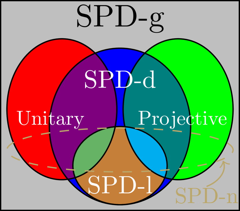
Figure 2: A schematic for the classification of SPD’s. The SPD-l has an interacting projector that is restricted to a local subspace. The SPD-d has an interacting projector which is composed of disjoint projectors. The SPD-g corresponds to a completely general interacting projector. The SPD-n is an SPD in which $\hat{\mathcal{V}}_{\tau}$ is restricted to n-particle operators. A unitary (projective) SPD is one in which the unrestricted projectors are unitary (Hermitian).

In summary, the SPD presents a systematic variational ansatz for studying quantum Hamiltonians. While the underlying idea behind the SPD was appreciated decades ago in the context of the generalizations of the Gutzwiller wave function[19], the general idea has not been fully exploited. A key advancement achieved by our discrete action theory is that the SPD can be formally understood in terms of an integer time Green’s function, which has a perfect parallel to the standard many-body Green’s function formalism, allowing one to generalize many of the existing ideas from many-body physics to the discrete action theory. It should be emphasized that the discrete action theory has very practical implications, such as allowing for the exact evaluation of SPD-d in infinite dimensions (see Subsection VI.2 for the proof).

II.4 Categorizing existing wave functions in terms of the SPD

In this subsection, we use the SPD to categorize existing variational wave function approaches within the literature (see Figure 3). We begin with the case of projective SPD’s, and first enumerate all G-type SPD’s. For $\mathcal{N}=1$, we have the well known Hartree-Fock approximation, given that Eq. 10 will result in the lowest energy single Slater determinant. For $\mathcal{N}=2$, the SPD-d recovers the Gutzwiller wave function[11, 12, 13]; the SPD-g recovers the variational coupled cluster (VCC) ansatz[37, 4]; the SPD-n recovers the Jastrow wave function[1, 34, 35, 2]. For $\mathcal{N}=3$, the SPD-d recovers the Gutzwiller-Baeriswyl wave function[18]. For the preceding two cases, variational quantum Monte-Carlo is typically used to evaluate the ansatz[38, 18, 39, 40, 2]. For $\mathcal{N}>3$, we are not aware of existing ansatz in the literature.

We now consider projective SPD’s of B-type. For $\mathcal{N}=1$, we are not aware of existing ansatz, which seems reasonable given that this would often amount to a crude approximation (see Subsection III.2.1 for an illustration). For $\mathcal{N}=2$, the SPD-d recovers a generalized version of the Baeriswyl wave function[41]. The SPD-d is more general given that the interacting projector is fully variational, whereas Baeriswyl made certain restrictions. For $\mathcal{N}=3$, the SPD-d recovers the Baeriswyl-Gutzwiller wave function[19]. For $\mathcal{N}>3$, we are not aware of existing ansatz in the literature.

We now consider the unitary SPD, and the most well known example is SPD-g for $\mathcal{N}=2$ in the case of the unitary coupled cluster (UCC) approach[3, 4, 5]. Due to the complexity of the Hamiltonians which are being studied with UCC, one cannot exactly evaluate the ansatz, resulting in applications to very small systems or uncontrolled approximations. For $\mathcal{N}>2$, there has recently been interest in the context of quantum computing. Farhi et al. proposed a Trotter-like ansatz composed of multiple unitary operations with the intent of evaluating it within a quantum computer[42]. These ideas were then extended and examined in the context of small Hubbard models[43]. A further generalization was made by Grimsley et al., where they considered pairs of non-interacting and two-particle interacting projectors[36]. All of these ansatz are pursued under the assumption that a quantum computer can be used to evaluate them.

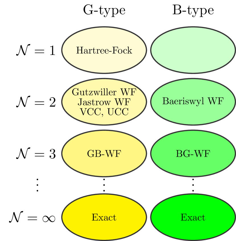
Figure 3: Existing variational wave functions (WF) classified in terms of the SPD, characterized by the number of integer time steps $\mathcal{N}$ and the type of SPD. The following acronyms are used: variation coupled cluster (VCC), unitary coupled cluster (UCC), Gutzwiller-Baeriswyl (GB), and Baeriswyl-Gutzwiller (BG).

II.5 Minimization of the total energy under the SPD

A key task in using any variational ansatz is to minimize the total energy with respect to the variational parameters. Given that there will typically be numerous variational parameters, it is critical to be able to compute the gradient of the energy with respect to the variational parameters. In this subsection, we demonstrate how to compute the gradient, which will showcase the emergence of integer time correlation functions.

To begin, we parameterize the non-interacting and interacting projectors as

$$\exp\left(\boldsymbol{\gamma}_{\tau}\left(\left\{c_{\tau i}\right\}\right)\cdot\hat{\bm{n}}\right), \hat{P}_{\tau}\left(\left\{g_{\tau i}\right\}\right),$$ (18)

where we have chosen a parameterization such that the derivatives have the following form

$$\frac{\partial\exp\left(\boldsymbol{\gamma}_{\tau}\left(\left\{c_{\tau i}\right\}\right)\cdot\hat{\bm{n}}\right)}{\partial c_{\tau i}}=\hat{K}_{\tau i}\exp\left(\boldsymbol{\gamma}_{\tau}\left(\left\{c_{\tau i}\right\}\right)\cdot\hat{\bm{n}}\right),$$ (19)

$$\frac{\partial\hat{P}_{\tau}\left(\left\{g_{\tau i}\right\}\right)}{\partial g_{\tau i}}=\hat{P}_{\tau}\left(\left\{g_{\tau i}\right\}\right)\hat{W}_{\tau i},$$ (20)

where $\hat{K}_{\tau i}$ and $\hat{W}_{\tau i}$ are operators which characterize the derivative. We note that this choice of parameterization is analogous to that of Sorella[40]. We can now compute the derivative of the energy as

$$\frac{\partial}{\partial c_{\tau i}}\langle\hat{H}\rangle_{\hat{\varrho}}=\frac{\partial}{\partial c_{\tau i}}\frac{\text{$\text{Tr}(\hat{\varrho}\hat{H}$)}}{\text{Tr}\left(\hat{\varrho}\right)}=$$

$$\langle\hat{K}_{\tau i}\left(\tau-1\right)\hat{H}\left(\mathcal{N}\right)\rangle_{\hat{\varrho}}-\langle\hat{K}_{\tau i}\left(\tau-1\right)\rangle_{\hat{\varrho}}\langle\hat{H}\left(\mathcal{N}\right)\rangle_{\hat{\varrho}},$$ (21)

$$\frac{\partial}{\partial g_{\tau i}}\langle\hat{H}\rangle_{\hat{\varrho}}=\frac{\partial}{\partial g_{\tau i}}\frac{\text{$\text{Tr}(\hat{\varrho}\hat{H})$}}{\text{Tr}(\hat{\varrho})}=$$

$$\langle\hat{W}_{\tau i}\left(\tau\right)\hat{H}\left(\mathcal{N}\right)\rangle_{\hat{\varrho}}-\langle\hat{W}_{\tau i}\left(\tau\right)\rangle_{\hat{\varrho}}\langle\hat{H}\left(\mathcal{N}\right)\rangle_{\hat{\varrho}},$$ (22)

where $\hat{O}(\tau)$ is an operator in the integer time Heisenberg representation defined as

$$\hat{O}(\tau) =\hat{U}_{\tau}\hat{O}\hat{U}_{\tau}^{-1}, \hat{U}_{\tau}=\hat{\mathcal{P}}_{1}\dots\hat{\mathcal{P}}_{\tau}.$$ (23)

This notion of integer time will be carefully introduced and explored in Sections III and IV. It should be noted that the second derivative can also be expressed in terms of integer time correlation functions, resulting in a new approximate saddle point for a given set of variational parameters. The fact that these derivatives can be evaluated in terms of computable correlation functions is critical to minimizing the total energy in practice.

III Integer Time Green’s function Formalism

III.1 Integer time correlation functions

While the SPD ansatz provides an intelligent route to approaching the exact solution, this form is only useful if it can be efficiently evaluated. Therefore, it will be essential to have a mathematical formalism which is conducive for developing robust approximations. We introduce the notation $\langle\hat{O}\rangle_{\hat{\rho}}=\textrm{Tr}(\hat{\rho}\hat{O})/\textrm{Tr}(\hat{\rho})$ for the measurement of some operator $\hat{O}$ under a density matrix $\hat{\rho}$. We begin by considering the expectation value of $\hat{O}$ under the SPD

$$\langle\hat{O}\rangle_{\hat{\varrho}} =\frac{\textrm{Tr}(\exp\left(\bm{\gamma}_{1}\cdot\hat{\bm{n}}\right)\hat{P}_{1}\dots\exp\left(\bm{\gamma}_{\mathcal{N}}\cdot\hat{\bm{n}}\right)\hat{P}_{\mathcal{N}}\hat{O})}{\textrm{Tr}(\exp\left(\bm{\gamma}_{1}\cdot\hat{\bm{n}}\right)\hat{P}_{1}\dots\exp\left(\bm{\gamma}_{\mathcal{N}}\cdot\hat{\bm{n}}\right)\hat{P}_{\mathcal{N}})}.$$ (24)

This expectation value can be re-expressed in the integer time interaction representation as

$$\langle\hat{O}\rangle_{\hat{\varrho}} =\frac{\langle\hat{P}_{1,I}(1)\hat{P}_{2,I}(2)\dots\hat{P}_{\mathcal{N},I}(\mathcal{N})\hat{O}_{I}(\mathcal{N})\rangle_{\hat{\varrho}_{0}}}{\langle\hat{P}_{1,I}(1)\hat{P}_{2,I}(2)\dots\hat{P}_{\mathcal{N},I}(\mathcal{N})\rangle_{\hat{\varrho}_{0}}},$$ (25)

where

$$\hat{\varrho}_{0}=\exp\left(\bm{\gamma}_{1}\cdot\hat{\bm{n}}\right)\dots\exp\left(\bm{\gamma}_{\mathcal{N}}\cdot\hat{\bm{n}}\right),$$ (26)

$$\hat{O}_{I}\left(\tau\right)=\hat{U}_{\tau;I}\hat{O}\hat{U}_{\tau;I}{}^{-1},$$ (27)

$$\hat{U}_{\tau;I}=\exp\left(\bm{\gamma}_{1}\cdot\hat{\bm{n}}\right)\dots\exp\left(\bm{\gamma}_{\tau}\cdot\hat{\bm{n}}\right),$$ (28)

where $\hat{\varrho}_{0}$ is the non-interacting SPD, the subscript $I$ denotes the integer time interaction representation, and $\tau=1,\dots,\mathcal{N}$. This interpretation of integer time evolution can be viewed as arising from a discrete action (see Subsection IV.1).

While this notion of integer time may appear artificial, it allows for a systematic evaluation using the integer time generalization of Wick’s theorem (see Appendix X.2 for a derivation). In the common scenario where the interacting projectors $\hat{P}_{i}$ will be the exponential of some interacting operator (see Eq. 9), it is natural to Taylor series expand such operators, yielding

$$\langle\hat{O}\rangle_{\hat{\varrho}} =\frac{\langle\textrm{T}\hat{P}_{1,I}(1)\hat{P}_{2,I}(2)\dots\hat{P}_{\mathcal{N},I}(\mathcal{N})\hat{O}_{I}(\mathcal{N})\rangle_{\hat{\varrho}_{0}}}{\langle\textrm{T}\hat{P}_{1,I}(1)\hat{P}_{2,I}(2)\dots\hat{P}_{\mathcal{N},I}(\mathcal{N})\rangle_{\hat{\varrho}_{0}}}$$ (29)

$$=\frac{\langle\textrm{T}\exp(\sum_{\tau=1}^{\mathcal{N}}\hat{\mathcal{V}}_{\tau,I}(\tau))\hat{O}_{I}(\mathcal{N})\rangle_{\hat{\varrho}_{0}}}{\langle\textrm{T}\exp(\sum_{\tau=1}^{\mathcal{N}}\hat{\mathcal{V}}_{\tau,I}(\tau))\rangle_{\hat{\varrho}_{0}}}$$ (30)

$$=\frac{\sum_{n=0}^{\infty}\frac{1}{n!}\langle\textrm{T}(\sum_{\tau=1}^{\mathcal{N}}\hat{\mathcal{V}}_{\tau,I}(\tau))^{n}\hat{O}_{I}(\mathcal{N})\rangle_{\hat{\varrho}_{0}}}{\sum_{n=0}^{\infty}\frac{1}{n!}\langle\textrm{T}(\sum_{\tau=1}^{\mathcal{N}}\hat{\mathcal{V}}_{\tau,I}(\tau))^{n}\rangle_{\hat{\varrho}_{0}}},$$ (31)

where the integer time ordering operator T first sorts the operators according to ascending integer time, and then according to the position in the original ordering of operators, and finally the result is presented from left to right; additionally, the resulting sign must be tracked when permuting Fermionic operators. It should be noted that our time convention is opposite to the usual definition[44]. It is useful to illustrate the integer time ordering operator with the example

$$\textrm{T}\hat{a}_{k,I}^{\dagger}(2)\hat{a}_{k^{\prime},I}(1)\hat{a}_{k,I}(2)=-\hat{a}_{k^{\prime},I}(1)\hat{a}_{k,I}^{\dagger}(2)\hat{a}_{k,I}(2).$$ (32)

Inspecting Eq. 31, it is clear that there are an infinite number of terms to be evaluated; and each term can be evaluated using the integer time Wick’s theorem (see Appendix III.2) in terms of the non-interacting integer time Green’s function

$$[\boldsymbol{g}_{0}]_{k\tau,k^{\prime}\tau^{\prime}}=\langle\text{T}\hat{a}_{k,I}^{\dagger}\left(\tau\right)a_{k^{\prime},I}\left(\tau^{\prime}\right)\rangle_{\hat{\varrho}_{0}},$$ (33)

where $k=1,\dots,L$ labels the spin-orbital index, and $\boldsymbol{g}_{0}$ is a matrix of dimension $L\mathcal{N}\times L\mathcal{N}$.

Having reformulated the expectation value of some operator in terms of integer time correlation functions, it becomes clear how to straightforwardly apply the integer time version of Wick’s theorem. This advancement will already allow us to exactly evaluate the SPD-l in terms of a finite number of diagrams (see Subsection III.2), allowing for the efficient and robust solution of the Anderson impurity model within VDAT[20]. Recently, Baeriswyl employed a perturbative approach to approximately evaluate a variant of the projective G-type SPD-d at $\mathcal{N}=3$ (as characterized from our general conventions) for the two dimensional Hubbard model[45]. Baeriswyl’s perturbative approach is recovered by our integer time formulation in the special case of $\mathcal{N}=3$ where we restrict Eq. 31 to second order, but our approach can naturally be applied at arbitrary $\mathcal{N}$ (it should be noted that $\tau$ is a variational parameter in Baeriswyl’s approach while $\tau$ is an integer time in ours).

III.2 Evaluating the SPD-l via Wick’s theorem

Having developed the integer time formalism, we already have the tools necessary to evaluate the SPD-l (see Eq. II), given that the interacting projector is confined to a subspace. Therefore, only a finite number of terms are required to evaluate an expectation value in this scenario, given as

$$\langle\hat{O}\rangle_{\hat{\varrho}}=$$

$$\frac{\sum_{\left\{\Gamma_{\tau}\Gamma^{\prime}_{\tau}\right\}}(\prod_{\tau}P_{\tau,\Gamma_{\tau}\Gamma^{\prime}_{\tau}})\langle\textrm{T}\prod_{\tau}\hat{X}_{\Gamma_{\tau}\Gamma^{\prime}_{\tau},I}(\tau)\hat{O}_{I}(\mathcal{N})\rangle_{\hat{\varrho}_{0}}}{\sum_{\left\{\Gamma_{\tau}\Gamma^{\prime}_{\tau}\right\}}(\prod_{\tau}P_{\tau,\Gamma_{\tau}\Gamma^{\prime}_{\tau}})\langle\textrm{T}\prod_{\tau}\hat{X}_{\Gamma_{\tau}\Gamma^{\prime}_{\tau},I}(\tau)\rangle_{\hat{\varrho}_{0}}},$$ (34)

where each term can be evaluated using the integer time Wick’s theorem (see Appendix X.2).

Given this capability of evaluating the SPD-l, we can already address many important Hamiltonians. For example, we can approximately solve the Anderson impurity model (AIM)[20]. For $\mathcal{N}=2$, the integer time formalism exactly evaluates the Gutzwiller wave function, which has long been available in the literature, but our $\mathcal{N}=3$ result had never been realized, and provides an accuracy comparable to the numerically exact density matrix renormalization group results[46] with relatively negligible computation cost. More generally, the above evaluation of the SPD-l allows us to evaluate the multi-orbital AIM, which we will address in future work.

We now consider pedagogical examples of the single orbital AIM with one bath site for $\mathcal{N}\leq 2$, evaluating unitary and projective SPD’s with G-type or B-type. Given that the exact solution can easily be evaluated by diagonalizing the Hamiltonian in the Fock space, this example provides a nice illustration of the evaluation of the SPD-l using the integer time Wick’s theorem.

III.2.1 Illustrative examples for $\mathcal{N}\leq 2$: Anderson impurity model with one bath

Here we study the AIM with only one bath orbital and particle-hole symmetry. The Hamiltonian is given as

$$\hat{H} =t\hat{K}+U\Delta\hat{d},$$ (35)

where

$$\hat{K}=\sum_{\sigma}(\hat{f}_{\sigma}^{\dagger}\hat{c}_{\sigma}+h.c.), \Delta\hat{d} =\prod_{\sigma}(\hat{f}_{\sigma}^{\dagger}\hat{f}_{\sigma}-\frac{1}{2}).$$ (36)

We first consider the case of $\mathcal{N}=1$ with a projective G-type SPD-l, given as

$$\hat{\varrho}=\exp(\gamma\hat{K}), \hat{P}_{1}=\hat{1},$$ (37)

where $\gamma$ is the non-interacting variational parameter. It will be inconvenient to use $\gamma$ directly given that it is not bounded, and therefore we can effectively reparameterize it with $\nu=\frac{1}{2}\tanh\left(\frac{\gamma}{2}\right)\in\left[-1/2,1/2\right]$ or $\gamma=2\text{$\tanh^{-1}\left(2\nu\right)$}$. As we have spin symmetry, we only need to compute the non-interacting integer time Green’s function for a given spin

$$\boldsymbol{g}_{\sigma;0}=\left(\begin{array}[]{cc}\frac{1}{2}&\nu\\ \nu&\frac{1}{2}\end{array}\right).$$ (40)

We can then use the integer time Wick’s theorem to compute the necessary integer time correlation functions required to evaluate the total energy

$$\langle\text{T}\hat{P}_{1,I}\left(1\right)\rangle_{\hat{\varrho}_{0}}=1,$$ (41)

$$\langle\text{T}\hat{P}_{1,I}\left(1\right)\Delta\hat{d}_{I}\left(1\right)\rangle_{\hat{\varrho}_{0}}=0,$$ (42)

$$\langle\text{T}\hat{P}_{1,I}\left(1\right)\hat{f}_{\sigma,I}^{\dagger}\left(1\right)\hat{c}_{\sigma,I}\left(1\right)\rangle_{\hat{\varrho}_{0}}=\nu.$$ (43)

The relevant expectation values can be obtained from the last time step, which is the only time step for $\mathcal{N}=1,$ as

$$\langle\hat{f}^{\dagger}\hat{c}\rangle_{\hat{\varrho}}=\nu, \langle\Delta\hat{d}\rangle_{\hat{\varrho}}=0.$$ (44)

Finally, the total energy can be written as

$$\mathcal{E} =\min_{\nu\in[-\frac{1}{2},\frac{1}{2}]}\left(4t\nu\right)=-2t.$$ (45)

We observe that $\mathcal{N}=1$ with a G-type SPD recovers the well known Hartree-Fock approximation, where the energy is independent of the Hubbard $U$ (given the chosen form of the interacting Hamiltonian).

We now move on to $\mathcal{N}=1$ with a B-type projective SPD-l, given as

$$\hat{\varrho}=\exp(g\Delta\hat{d}), \hat{P}_{1}=\exp(g\Delta\hat{d})=(\hat{1}+u\Delta\hat{d}).$$ (46)

Here we reparameterize the interacting variational parameter $g$ in terms of $u\in[-4,4]$. We proceed by constructing the non-interacting integer time Green’s function

$$\boldsymbol{g}_{0;\sigma}=\left(\begin{array}[]{cc}\frac{1}{2}&0\\ 0&\frac{1}{2}\end{array}\right),$$ (47)

and compute all the necessary integer time matrix elements

$$\langle\textrm{T}\hat{P}_{1,I}(1)\rangle_{\hat{\varrho}_{0}}=1,$$ (48)

$$\langle\textrm{T}\hat{P}_{1,I}(1)\Delta\hat{d}_{I}(1)\rangle_{\hat{\varrho}_{0}}=\frac{u}{16},$$ (49)

$$\langle\textrm{T}\hat{P}_{1,I}(1)\hat{f}_{\sigma,I}^{\dagger}(1)\hat{c}_{\sigma,I}(1)\rangle_{\hat{\varrho}_{0}}=0.$$ (50)

The relevant expectation values can be obtained as

$$\langle\hat{f}^{\dagger}\hat{c}\rangle_{\hat{\varrho}}=0, \langle\Delta\hat{d}\rangle_{\hat{\varrho}}=\frac{u}{16}.$$ (51)

The resulting total energy is then

$$\mathcal{E} =\min_{u\in\left[-4,4\right]}\left(U\frac{u}{16}\right)=-\frac{U}{4}.$$ (52)

Here we see that the energy is independent of the hopping parameter, given that this ansatz amounts to a collection of two decoupled atoms.

We now move on to $\mathcal{N}=2$ for the G-type projective SPD-l, given as

$$\hat{\varrho}=\exp(g\Delta\hat{d})\exp(\gamma\hat{K})\exp(g\Delta\hat{d}),$$ (53)

where the interacting projector is

$$\hat{P}_{1}=\hat{P}_{2}=\exp(g\Delta\hat{d})=(\hat{1}+u\Delta\hat{d}),$$ (54)

and $\gamma$ is reparameterized with $\nu$ as before, and there is no restriction on $u$ given that it occupies the outermost position in the SPD. The noninteracting integer time Green’s function is then

$$\boldsymbol{g}_{\sigma;0}=\left(\begin{array}[]{cccc}\frac{1}{2}&\nu&\frac{1}{2}&-\nu\\ \nu&\frac{1}{2}&-\nu&\frac{1}{2}\\ -\frac{1}{2}&-\nu&\frac{1}{2}&\nu\\ -\nu&-\frac{1}{2}&\nu&\frac{1}{2}\end{array}\right),$$ (59)

where we have used integer time major ordering of the basis, where integer time is the slow index and goes in ascending order and the orbital is the fast index and goes from $f$ to $c$, resulting in the four sequential indices $(f,1),(c,1),(f,2),(c,2)$. For example, we have $[\boldsymbol{g}_{\sigma;0}]_{13}=\langle\textrm{T}\hat{f}_{I}^{\dagger}(1)\hat{f}_{I}(2)\rangle_{\hat{\varrho}_{0}}$, etc. The necessary integer time correlation functions needed to compute the total energy are

$$\langle\text{T}\hat{P}_{1,I}\left(1\right)\hat{P}_{2,I}\left(2\right)\rangle_{\hat{\varrho}_{0}}=\frac{u^{2}}{16}+1,$$ (60)

$$\langle\text{T}\hat{P}_{1,I}\left(1\right)\hat{P}_{2,I}\left(2\right)\Delta\hat{d}_{I}\left(2\right)\rangle_{\hat{\varrho}_{0}}=\frac{u}{8},$$ (61)

$$\langle\text{T}\hat{P}_{1,I}\left(1\right)\hat{P}_{2,I}\left(2\right)\hat{f}_{\sigma,I}^{\dagger}\left(2\right)\hat{c}_{\sigma,I}\left(2\right)\rangle_{\hat{\varrho}_{0}}=\frac{-\nu}{16}(u^{2}-16).$$ (62)

The relevant expectation values can be obtained as

$$\langle\hat{f}^{\dagger}\hat{c}\rangle_{\hat{\varrho}}=\frac{16-u^{2}}{16+u^{2}}\nu, \langle\Delta\hat{d}\rangle_{\hat{\varrho}}=\frac{2u}{u^{2}+16}.$$ (63)

The ground state energy can then be obtained as

$$\mathcal{E} =\min_{\nu\in[-\frac{1}{2},\frac{1}{2}],u}\left(4t\nu\frac{16-u^{2}}{16+u^{2}}+U\frac{2u}{u^{2}+16}\right)$$

$$=\min_{u}\left(-2t\frac{16-u^{2}}{16+u^{2}}+U\frac{2u}{u^{2}+16}\right)$$

$$=-\frac{1}{4}\sqrt{64t^{2}+U^{2}}.$$

Notice that in this simple single bath case, $\mathcal{N}=2$ with the G-type projective SPD-l provides the exact ground state energy.

We now consider the B-type projective SPD-l for $\mathcal{N}=2$, given as

$$\hat{\varrho}=\exp(\gamma\hat{K})\exp(g\Delta\hat{d})\exp(\gamma\hat{K}),$$ (64)

where the interacting projectors are

$$\hat{P}_{1}=\exp(g\Delta\hat{d})=(\hat{1}+u\Delta\hat{d}), \hat{P}_{2}=\hat{1},$$ (65)

and we reparameterize $\gamma$ as in the previous case, though $\nu\in\left[-\infty,\infty\right]$ given that the non-interacting projector is in the outer position of the SPD; in addition to reparameterizing $g$ in terms of $u$, though here the interacting projector is in the center position of the SPD and therefore $u\in[-4,4]$. We can proceed by constructing the non-interacting integer time Green’s function

$$\boldsymbol{g}_{0;\sigma}=\left(\begin{array}[]{cccc}\frac{1}{2}&\frac{2\nu}{4\nu^{2}+1}&\frac{1-4\nu^{2}}{8\nu^{2}+2}&0\\ \frac{2\nu}{4\nu^{2}+1}&\frac{1}{2}&0&\frac{1-4\nu^{2}}{8\nu^{2}+2}\\ \frac{4\nu^{2}-1}{8\nu^{2}+2}&0&\frac{1}{2}&\frac{2\nu}{4\nu^{2}+1}\\ 0&\frac{4\nu^{2}-1}{8\nu^{2}+2}&\frac{2\nu}{4\nu^{2}+1}&\frac{1}{2}\end{array}\right).$$ (66)

We then compute all the necessary matrix elements

$$\langle\textrm{T}\hat{P}_{1,I}(1)\rangle_{\hat{\varrho}_{0}}=1,$$ (67)

$$\langle\textrm{T}\hat{P}_{1,I}(1)\Delta\hat{d}_{I}(2)\rangle_{\hat{\varrho}_{0}}=\frac{\left(1-4\nu^{2}\right)^{4}u}{16\left(4\nu^{2}+1\right)^{4}},$$ (68)

$$\langle\textrm{T}\hat{P}_{1,I}(1)\hat{f}_{\sigma,I}^{\dagger}(2)\hat{c}_{\sigma,I}(2)\rangle_{\hat{\varrho}_{0}}=\frac{2\nu}{4\nu^{2}+1}.$$ (69)

The relevant expectation values can then be obtained as

$$\langle\hat{f}^{\dagger}\hat{c}\rangle_{\hat{\varrho}}=\frac{2\nu}{4\nu^{2}+1}, \langle\Delta\hat{d}\rangle_{\hat{\varrho}}=\frac{\left(1-4\nu^{2}\right)^{4}u}{16\left(4\nu^{2}+1\right)^{4}}.$$ (70)

The resulting total energy is then

$$\mathcal{E} =\min_{u\in\left[-4,4\right],\nu}\left(t\frac{8\nu}{4\nu^{2}+1}+U\frac{\left(1-4\nu^{2}\right)^{4}u}{16\left(4\nu^{2}+1\right)^{4}}\right),$$ (71)

$$=\min_{\nu}\left(\frac{8\nu t}{4\nu^{2}+1}-\frac{\left(1-4\nu^{2}\right)^{4}U}{4\left(4\nu^{2}+1\right)^{4}}\right).$$ (72)

The saddle points are then found by individually solving the following two equations

$$\left(4\nu^{2}+1\right)^{3}t+2\nu\left(1-4\nu^{2}\right)^{2}U =0, \left(4\nu^{2}-1\right)=0.$$ (73)

For the former, we have

$$U =-\frac{\left(4\nu^{\star 2}+1\right)^{3}t}{2\nu^{\star}\left(1-4\nu^{\star 2}\right)^{2}}, \mathcal{E}=\frac{\left(16\nu^{\star 4}+56\nu^{\star 2}+1\right)t}{8\left(4\nu^{\star 3}+\nu^{\star}\right)}.$$ (74)

The ground state energy can then be written as

$$\mathcal{E}=\bigg{\{}\begin{array}[]{cc}\frac{\left(16\nu^{\star 4}+56\nu^{\star 2}+1\right)t}{8\left(4\nu^{\star 3}+\nu^{\star}\right)},&U\geq 6.75t\\ -2t,&U\leq 6.75t\end{array}$$ (75)

where for $U\leq 6.75t$, the B-type $\mathcal{N}=2$ projective SPD gives the same energy as the G-type $\mathcal{N}=1$ projective SPD.

We summarize the results for the ground state energy as a function of $U/t$ in these four cases in Figure 4. As noted above, the $\mathcal{N}=2$ G-type projective SPD (i.e. the Gutzwiller wave function) gives the exact solution in this case. The $\mathcal{N}=2$ B-type projective SPD is interesting given that is has multiple saddle points, foreshadowing the possibility of becoming stuck in a false minimum when minimizing the energy. Another point illustrated by this plot is that larger $\mathcal{N}$ always has a lower ground state energy, as it must.

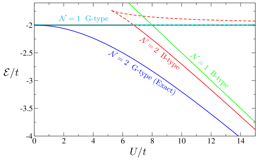
Figure 4: Ground state energy as a function of $U/t$ for the single orbital AIM with one bath site using VDAT for $\mathcal{N}=1,2$, with both G-type and B-type projective SPD-l. Dotted lines denote higher energy saddle points, while solid lines denote the ground state energy for a given $\mathcal{N}$.

All of the above cases have been for projective SPD-l, and now we consider unitary SPD-l. For $\mathcal{N}=1$, there is no difference between the projective and unitary case, so we begin with $\mathcal{N}=2$ G-type with an SPD given as

$$\hat{\varrho}=\exp(ig\Delta\hat{d})\exp(\gamma\hat{K})\exp(-ig\Delta\hat{d}),$$ (76)

where $g$ is a real number and the unconstrained projector is unitary. We reparameterize the interacting projector as

$$\hat{P}_{1} =1+iu\Delta\hat{d}=\hat{P}_{2}^{\dagger}.$$ (77)

The non-interacting integer time Green’s function is the same as in the projective case, given in Eq. 59. The integer time correlation functions needed to compute the total energy are

$$\langle\text{T}\hat{P}_{1,I}\left(1\right)\hat{P}_{2,I}\left(2\right)\rangle_{\hat{\varrho}_{0}}=\frac{u^{2}}{16}+1,$$ (78)

$$\langle\text{T}\hat{P}_{1,I}\left(1\right)\hat{P}_{2,I}\left(2\right)\Delta\hat{d}_{I}\left(2\right)\rangle_{\hat{\varrho}_{0}}=0,$$ (79)

$$\langle\text{T}\hat{P}_{1,I}\left(1\right)\hat{P}_{2,I}\left(2\right)\hat{f}_{\sigma,I}^{\dagger}\left(2\right)\hat{c}_{\sigma,I}\left(2\right)\rangle_{\hat{\varrho}_{0}}=\frac{-\nu}{16}(u^{2}-16).$$ (80)

The relevant expectation values can be obtained as

$$\langle\hat{f}^{\dagger}\hat{c}\rangle_{\hat{\varrho}}=\frac{16-u^{2}}{16+u^{2}}\nu, \langle\Delta\hat{d}\rangle_{\hat{\varrho}}=0.$$ (81)

The ground state energy can then be obtained as

$$\mathcal{E} =\min_{\nu\in[-\frac{1}{2},\frac{1}{2}],u}\left(4t\nu\frac{16-u^{2}}{16+u^{2}}\right)=-2t,$$ (82)

which is identical to $\mathcal{N}=1$ for the projective G-type case. Similarly, for the unitary case of the B-type at $\mathcal{N}=2$, the result is identical to the projective B-type at $\mathcal{N}=1$.

The unitary case for the G-type at $\mathcal{N}=3$ does indeed recover the exact solution (details not shown), similar to the projective case for the G-type at $\mathcal{N}=2$. Therefore, we see that the projective SPD is clearly superior to the unitary SPD in this Hamiltonian. This same trend was found when comparing the variational coupled cluster approach, which is a projective SPD, and the unitary coupled cluster approach, which is a unitary SPD, in the context of the Lipkin Hamiltonian[47].

IV The Discrete Action Theory

IV.1 Introducing and categorizing the discrete action

We have illustrated that the SPD can be evaluated using only the non-interacting integer time Green’s function and the integer time Wick’s theorem, allowing for the efficient evaluation of the SPD-l (see Section III). However, this path forward will not be able to extend to more complex scenarios such as SPD-d, where the interacting projector is not strictly local, which will require the summation of an infinite number of diagrams. A more sophisticated approach is needed, which motivates the introduction of a discrete action.

We begin by introducing both the integer time Heisenberg and Schrodinger representations. As discussed in Subsection III.1, the integer time evolution in the integer time interaction representation is defined as

$$\hat{O}_{I}\left(\tau\right)=\hat{U}_{\tau;I}\hat{O}\hat{U}_{\tau;I}{}^{-1},$$ (83)

$$\hat{U}_{\tau;I}=\exp\left(\bm{\gamma}_{1}\cdot\hat{\bm{n}}\right)\dots\exp\left(\bm{\gamma}_{\tau}\cdot\hat{\bm{n}}\right),$$ (84)

where $\tau=1,\dots,\mathcal{N}$. The integer time Green’s function under an SPD in the integer time interaction representation is then

$$[\boldsymbol{g}]_{k\tau,k^{\prime}\tau^{\prime}} =\frac{\langle\text{T}\big{(}\prod_{\tau=1}^{\mathcal{N}}\hat{P}_{\tau,I}(\tau)\big{)}\hat{a}_{k,I}^{\dagger}\left(\tau\right)\hat{a}_{k^{\prime},I}\left(\tau^{\prime}\right)\rangle_{\hat{\varrho}_{0}}}{\langle\text{T}\big{(}\prod_{\tau=1}^{\mathcal{N}}\hat{P}_{\tau,I}(\tau)\big{)}\rangle_{\hat{\varrho}_{0}}},$$ (85)

where $\tau=1,\dots,\mathcal{N}$ and $k=1,\dots,L$. Therefore, $\boldsymbol{g}$ is a matrix of dimension $L\mathcal{N}\times L\mathcal{N}$, and plays a similar role to the usual many-particle Green’s function.

In the integer time Heisenberg representation, integer time evolution of operators is given as

$$\hat{O}(\tau) =\hat{U}_{\tau}\hat{O}\hat{U}_{\tau}^{-1}, \hat{U}_{\tau}=\hat{\mathcal{P}}_{1}\dots\hat{\mathcal{P}}_{\tau}.$$ (86)

The integer time Green’s function under an SPD in the integer time Heisenberg representation is then

$$[\boldsymbol{g}]_{k\tau,k^{\prime}\tau^{\prime}} =\langle\text{T}\hat{a}_{k}^{\dagger}\left(\tau\right)\hat{a}_{k^{\prime}}\left(\tau^{\prime}\right)\rangle_{\hat{\varrho}}.$$ (87)

In the integer time Schrodinger representation, integer time evolution is defined as

$$\hat{O}_{S}(\tau)=\hat{O},$$ (88)

where the time index now only serves the purpose of tracking which integer time an operator is associated with, such that time ordering can be performed. The integer time Green’s function under an SPD in the integer time Schrodinger representation is then

$$[\boldsymbol{g}]_{k\tau,k^{\prime}\tau^{\prime}} =\frac{\langle\text{T}\big{(}\prod_{\tau=1}^{\mathcal{N}}\hat{\mathcal{P}}_{\tau,S}(\tau)\big{)}\hat{a}_{k,S}^{\dagger}\left(\tau\right)\hat{a}_{k^{\prime},S}\left(\tau^{\prime}\right)\rangle_{\hat{1}}}{\langle\text{T}\big{(}\prod_{\tau=1}^{\mathcal{N}}\hat{\mathcal{P}}_{\tau,S}(\tau)\big{)}\rangle_{\hat{1}}},$$ (89)

A more general integer time correlation function under the SPD can be represented in the Heisenberg, interaction, and Schrodinger representation, respectively, as

$$\langle\textrm{T}\hat{O}_{1}(\tau_{1})\dots\hat{O}_{M}(\tau_{M})\rangle_{\hat{\varrho}}$$

$$=\frac{\langle\textrm{T}\big{(}\prod_{\tau=1}^{\mathcal{N}}\hat{P}_{\tau,I}(\tau)\big{)}\hat{O}_{1,I}(\tau_{1})\dots\hat{O}_{M,I}(\tau_{M})\rangle_{\hat{\varrho}_{0}}}{\langle\textrm{T}\big{(}\prod_{\tau=1}^{\mathcal{N}}\hat{P}_{\tau,I}(\tau)\big{)}\rangle_{\hat{\varrho}_{0}}}$$ (90)

$$=\frac{\langle\textrm{T}\big{(}\prod_{\tau=1}^{\mathcal{N}}\hat{\mathcal{P}}_{\tau,S}(\tau)\big{)}\hat{O}_{1,S}(\tau_{1})\dots\hat{O}_{M,S}(\tau_{M})\rangle_{\hat{1}}}{\langle\textrm{T}\big{(}\prod_{\tau=1}^{\mathcal{N}}\hat{\mathcal{P}}_{\tau,S}(\tau)\big{)}\rangle_{\hat{1}}}.$$ (91)

We therefore have the three standard pictures for describing integer time correlations.

We now introduce the most general integer time correlation function, which is not necessarily associated with an SPD, and this is most naturally expressed in the Schrodinger represenation as

$$\frac{\langle\textrm{T}\hat{\mathcal{A}}\hat{O}_{1,S}(\tau_{1})\dots\hat{O}_{M,S}(\tau_{M})\rangle_{\hat{1}}}{\langle\textrm{T}\hat{\mathcal{A}}\rangle_{\hat{1}}},$$ (92)

where $\mathbb{\hat{\mathcal{A}}}$ is a discrete action (DA) which characterizes all possible integer time correlations for a given $\mathcal{N}$ and is defined as

$$\hat{\mathcal{A}}=\sum_{\begin{subarray}{c}\eta_{1}..\eta_{\mathcal{N}}\\ \eta^{\prime}_{1}...\eta^{\prime}_{\mathcal{N}}\end{subarray}}\mathcal{A}_{\eta_{1}..\eta_{\mathcal{N}},\eta^{\prime}_{1}..\eta^{\prime}_{\mathcal{N}}}\hat{X}_{\eta_{1}\eta^{\prime}_{1},S}\left(1\right)...\hat{X}_{\eta_{\mathcal{N}}\eta^{\prime}_{\mathcal{N}},S}\left(\mathcal{N}\right),$$ (93)

where $\hat{X}_{\Gamma\Gamma^{\prime}}=|\Gamma\rangle\langle\Gamma^{\prime}|$ is a Hubbard operator, $\{|\eta_{\tau}\rangle\}$ forms an orthonormal basis for the Fock space, and $\mathcal{A}_{\eta_{1}..\eta_{\mathcal{N}},\eta^{\prime}_{1}..\eta^{\prime}_{\mathcal{N}}}$ is the discrete action represented in the given basis. In the case of the SPD, the discrete action is a product of $\mathcal{N}$ distinct operators

$$\hat{\mathcal{A}}=\hat{\mathcal{P}}_{1,S}(1)\dots\hat{\mathcal{P}}_{\mathcal{N},S}(\mathcal{N}).$$ (94)

Given a system with $L$ spin orbitals, a general discrete action for $\mathcal{N}$ integer time steps will contain at most $4^{L\mathcal{N}}$ nonzero entries, which is exponentially larger than the discrete action of an SPD where there are at most $4^{L}\mathcal{N}$ nonzero entries. The more general discrete action will prove useful in practical applications.

We now categorize the common types of discrete actions, which can naturally be broken down into three varieties (see Figure 5 for a schematic): sequential discrete actions (SDA), canonical discrete actions (CDA), and general discrete actions (GDA). We start with GDA, which is defined as

$$\hat{\mathcal{A}}=\hat{\mathcal{A}}_{0}\hat{P},\hskip 10.00002pt\hat{\mathcal{A}}_{0}=\hat{\mathcal{A}}_{G}(\boldsymbol{g}_{0}),$$ (95)

$$\hat{\mathcal{A}}_{G}(\boldsymbol{g}_{0})=\exp([\boldsymbol{v}_{Q}(\boldsymbol{g}_{0})]_{k\tau,k^{\prime}\tau^{\prime}}\hat{a}_{k,S}^{\dagger}(\tau)\hat{a}_{k^{\prime},S}(\tau^{\prime})),$$ (96)

$$\hat{P}=P_{\eta_{1}..\eta_{\mathcal{N}},\eta^{\prime}_{1}..\eta^{\prime}_{\mathcal{N}}}\hat{X}_{\eta_{1}\eta^{\prime}_{1},S}\left(1\right)...\hat{X}_{\eta_{\mathcal{N}}\eta^{\prime}_{\mathcal{N}},S}\left(\mathcal{N}\right),$$ (97)

$$\boldsymbol{v}_{Q}(\boldsymbol{g}_{0})=\ln((\boldsymbol{g}_{0}^{-1}-1)^{-1}(\boldsymbol{g}_{Q}^{-1}-1))^{T},$$ (98)

$$[\boldsymbol{g}_{Q}]_{k\tau,k^{\prime}\tau^{\prime}}=\langle\text{T}\hat{a}_{k,S}^{\dagger}\left(\tau\right)\hat{a}_{k^{\prime},S}\left(\tau^{\prime}\right)\rangle_{\hat{1}},$$ (99)

where the Einstein summation convention has been used, and the derivation of Eq. 98 is given in Subsection IV.2. Therefore, we see that the GDA is composed of a non-interacting discrete action $\hat{\mathcal{A}}_{0}$ and an interacting projector $\hat{P}$, where both have no constraint with respect to the integer time structure.

The CDA is a GDA by restricting the interacting projector into a time blocked form as

$$\hat{P} =\prod_{\tau=1}^{\mathcal{N}}\hat{P}_{\tau,S}(\tau),$$ (100)

which will be very useful in evaluating the SPD-d (see Section VI). Finally, the SDA is the discrete action corresponding to an SPD, which can be viewed as a CDA by restricting the non-interacting discrete action into the following form

$$\hat{\mathcal{A}}_{0}=\exp(\sum_{\tau=1}^{\mathcal{N}}\boldsymbol{\gamma}_{\tau}\cdot\hat{\bm{n}}_{S}(\tau)),$$ (101)

where $\hat{\bm{n}}$ was defined in Eq. 6.

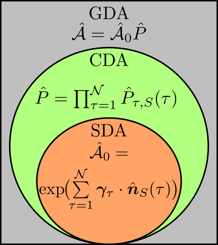
Figure 5: A schematic for the classification of discrete actions. The SDA is the discrete action corresponding to an SPD. The CDA is the discrete action where the corresponding non-interacting discrete action is integer time mixed. The GDA is a completely general discrete action. The SDA is a subset of the CDA, which is a subset of the GDA.

The form of the CDA and GDA requires the evaluation of an integer time ordered expression with nontrivial integer time structure, which is inconvenient to manipulate. Therefore, it is useful to develop a more adept mathematical framework which is conducive to handling such scenarios. This motivates the introduction of the compound space, which is the topic of the next subsection.

IV.2 Integer time path integral and the compound space

Here we prescribe a mathematical formalism to recast the integer time ordered correlations of a general discrete action as a static measurement under an effective density matrix in a compound quantum system. This can be viewed as a reformulation of the path integral. In the usual path integral formalism, one can interpret the action as the effective energy of a classical system (though for Fermions one needs Grassmann numbers, which have no classical counterpart) with the same spatial structure and one more dimension for the time correlation[48]. Thus, we have the well-known fact that $d$ dimensional quantum fields correspond to a ($d$+1) dimensional classical system. In the following, we reformulate this mapping, resulting in two key differences. First, as the number of time steps is finite, the number of points within the extra dimension is also finite. Second, for the evolution of each time step, we need to retain an exact operator form given that the $\mathcal{\hat{P}}_{i}$ can not be treated as an infinitesimally small expansion from the identity matrix. As a result, we obtain a compound quantum system with a Fock space of $\mathbb{H}_{c}=\otimes_{\tau=1}^{\mathcal{N}}\mathbb{H}$, where $\mathbb{H}$ is the Fock space of the original system.

To begin, we must define how we represent operators from the original system in the compound system. Each creation and destruction operator will be attached to a given integer time index when promoted to the compound space. For example, for a system with $L$ spin orbitals, any operator can be built algebraically from the $2L$ operators $\hat{a}_{1}^{\dagger},\dots,\hat{a}_{L}^{\dagger}$ and $\hat{a}_{1},\dots,\hat{a}_{L}$. Given $\mathcal{N}$ time steps, any operator for the compound system can be built algebraically from $2L\mathcal{N}$ operators $\textrm{\@text@baccent{$\hat{a}$}}_{1}^{\dagger(1)},\dots,\textrm{\@text@baccent{$\hat{a}$}}_{L}^{\dagger(1)},\dots,\textrm{\@text@baccent{$\hat{a}$}}_{1}^{\dagger(\tau)},\dots,\textrm{\@text@baccent{$\hat{a}$}}_{L}^{\dagger(\tau)},\dots,\textrm{\@text@baccent{$\hat{a}$}}_{1}^{\dagger(\mathcal{N})},\dots,\textrm{\@text@baccent{$\hat{a}$}}_{L}^{\dagger(\mathcal{N})}$ and $\textrm{\@text@baccent{$\hat{a}$}}_{1}^{(1)},\dots,\textrm{\@text@baccent{$\hat{a}$}}_{L}^{(1)},\dots,\textrm{\@text@baccent{$\hat{a}$}}_{1}^{(\tau)},\dots,\textrm{\@text@baccent{$\hat{a}$}}_{L}^{(\tau)},\dots,\textrm{\@text@baccent{$\hat{a}$}}_{1}^{(\mathcal{N})},\dots,\textrm{\@text@baccent{$\hat{a}$}}_{L}^{(\mathcal{N})}$ , where the underscore denotes an operator in the compound space, and the superscript $\tau$ associates the operator with integer time $\tau$. These operators in the compound space must obey the Fermionic anti-commutation relations, yielding

$$\left\{\textrm{\@text@baccent{$\hat{a}$}}_{k}^{\dagger(\tau)},\textrm{\@text@baccent{$\hat{a}$}}_{k^{\prime}}^{(\tau^{\prime})}\right\}=\delta_{kk^{\prime}}\delta_{\tau\tau^{\prime}},$$ (102)

$$\left\{\textrm{\@text@baccent{$\hat{a}$}}_{k}^{(\tau)},\textrm{\@text@baccent{$\hat{a}$}}_{k^{\prime}}^{(\tau^{\prime})}\right\}=\left\{\textrm{\@text@baccent{$\hat{a}$}}_{k}^{\dagger(\tau)},\textrm{\@text@baccent{$\hat{a}$}}_{k^{\prime}}^{\dagger(\tau^{\prime})}\right\}=0.$$ (103)

The commutation relations indicate that the time index has the same behavior as the orbital index in the compound space. In order to promote some generic operator $\hat{O}=f(\hat{a}_{1}^{\dagger},\dots,\hat{a}_{L}^{\dagger},\hat{a}_{1},\dots,\hat{a}_{L})$ associated with a given $\tau$, we obtain the corresponding operator in the compound space as $\textrm{\@text@baccent{$\hat{O}$}}^{(\tau)}=f(\textrm{\@text@baccent{$\hat{a}$}}_{1}^{\dagger(\tau)},\dots,\textrm{\@text@baccent{$\hat{a}$}}_{L}^{\dagger(\tau)},\textrm{\@text@baccent{$\hat{a}$}}_{1}^{(\tau)},\dots,\textrm{\@text@baccent{$\hat{a}$}}_{L}^{(\tau)})$.

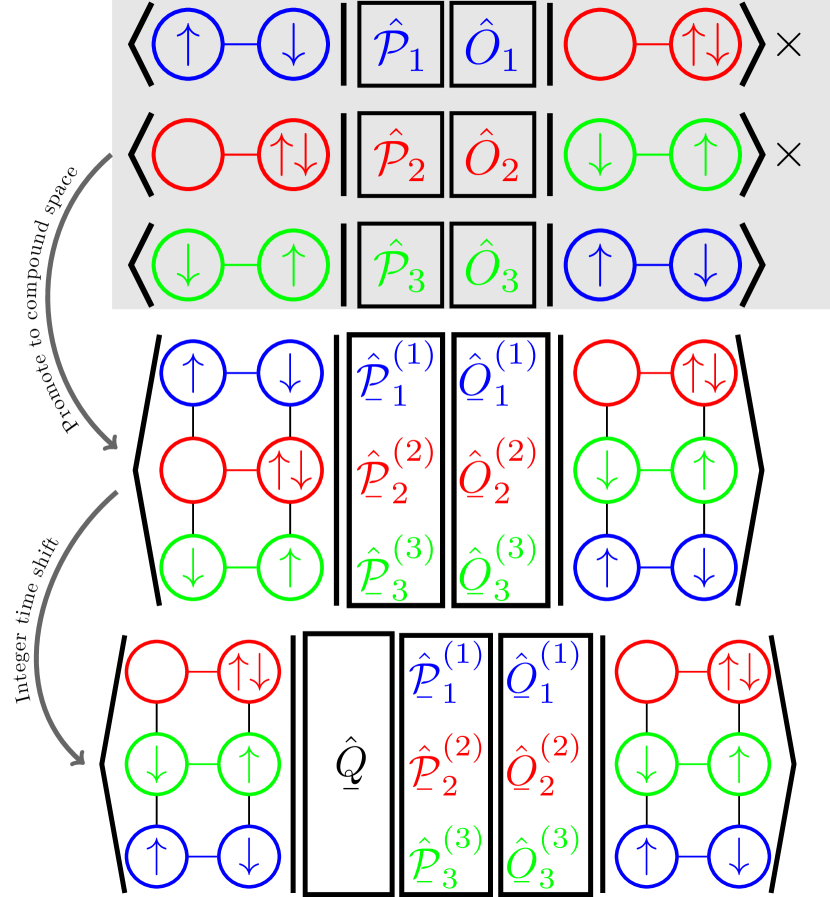
Figure 6: A schematic of the integer time path integral which derives a map to the compound space, using the example of the Hubbard dimer for $\mathcal{N}=3$. The first step denotes a particular snapshot within Eq. 105. The second step merges the state vectors from different time steps into the compound space, while the operators are promoted, illustrating Eq. 109. The final step illustrates the integer time shift operator $̱\hat{Q}$, which results in a diagonal matrix element, corresponding to Eq. 111.

Now we proceed to derive the mapping to the compound space in the special case of the SPD (see Figure 6 for a schematic of the following derivation). Considering a general integer time correlation function under the SPD and performing $\mathcal{N}$ identity insertions

$$\langle\textrm{T}\hat{O}_{1}(1)\dots\hat{O}_{\mathcal{N}}(\mathcal{N})\rangle_{\hat{\varrho}}=\textrm{Tr}(\hat{\mathcal{P}}_{1}\hat{O}_{1}\dots\hat{\mathcal{P}}_{\mathcal{N}}\hat{O}_{\mathcal{N}})/\textrm{Tr}(\hat{\mathcal{P}}_{1}\dots\hat{\mathcal{P}}_{\mathcal{N}})$$ (104)

$$=\frac{1}{C}\sum_{\Gamma_{1}\dots\Gamma_{\mathcal{N}}}\langle\Gamma_{1}|\exp(\bm{\gamma}_{1}\cdot\hat{\bm{n}})\hat{P}_{1}\hat{O}_{1}|\Gamma_{2}\rangle\langle\Gamma_{2}|\exp(\bm{\gamma}_{2}\cdot\hat{\bm{n}})\hat{P}_{2}\hat{O}_{2}|\Gamma_{3}\rangle\dots\langle\Gamma_{\mathcal{N}}|\exp(\bm{\gamma}_{\mathcal{N}}\cdot\hat{\bm{n}})\hat{P}_{\mathcal{N}}\hat{O}_{\mathcal{N}}|\Gamma_{1}\rangle$$ (105)

$$=\frac{1}{C}\sum_{\Gamma_{1}\dots\Gamma_{\mathcal{N}}}\langle\Gamma_{1}|\left(\sum_{\Gamma\Gamma^{\prime}}c_{1;\Gamma\Gamma^{\prime}}\hat{X}_{\Gamma\Gamma^{\prime}}\right)|\Gamma_{2}\rangle\langle\Gamma_{2}|\left(\sum_{\Gamma\Gamma^{\prime}}c_{2;\Gamma\Gamma^{\prime}}\hat{X}_{\Gamma\Gamma^{\prime}}\right)|\Gamma_{3}\rangle\dots\langle\Gamma_{\mathcal{N}}|\left(\sum_{\Gamma\Gamma^{\prime}}c_{\mathcal{N};\Gamma\Gamma^{\prime}}\hat{X}_{\Gamma\Gamma^{\prime}}\right)|\Gamma_{1}\rangle$$ (106)

$$=\frac{1}{C}\sum_{\Gamma_{1}\dots\Gamma_{\mathcal{N}}}c_{1;\Gamma_{1}\Gamma_{2}}c_{2;\Gamma_{2}\Gamma_{3}}\dots c_{\mathcal{N};\Gamma_{\mathcal{N}}\Gamma_{1}}\frac{\langle\Gamma_{1}\otimes\Gamma_{2}\dots\otimes\Gamma_{\mathcal{N}}|\textrm{\@text@baccent{$\hat{X}$}}_{\Gamma_{1}\Gamma_{2}}^{(1)}\textrm{\@text@baccent{$\hat{X}$}}_{\Gamma_{2}\Gamma_{3}}^{(2)}\dots\textrm{\@text@baccent{$\hat{X}$}}_{\Gamma_{\mathcal{N}}\Gamma_{1}}^{(\mathcal{N})}|\Gamma_{2}\otimes\Gamma_{3}\dots\otimes\Gamma_{1}\rangle}{\langle\Gamma_{1}\otimes\Gamma_{2}\dots\otimes\Gamma_{\mathcal{N}}|\textrm{\@text@baccent{$\hat{X}$}}_{\Gamma_{1}\Gamma_{2}}^{(1)}\textrm{\@text@baccent{$\hat{X}$}}_{\Gamma_{2}\Gamma_{3}}^{(2)}\dots\textrm{\@text@baccent{$\hat{X}$}}_{\Gamma_{\mathcal{N}}\Gamma_{1}}^{(\mathcal{N})}|\Gamma_{2}\otimes\Gamma_{3}\dots\otimes\Gamma_{1}\rangle}$$ (107)

$$=\frac{1}{C}\sum_{\Gamma_{1}...\Gamma_{\mathcal{N}}}\theta_{\Gamma_{2}\Gamma_{3}...\Gamma_{1}}\langle\Gamma_{1}\otimes\Gamma_{2}...\otimes\Gamma_{\mathcal{N}}|\left(\sum_{\Gamma\Gamma^{\prime}}c_{1;\Gamma\Gamma^{\prime}}\textrm{\@text@baccent{$\hat{X}$}}_{\Gamma\Gamma^{\prime}}^{(1)}\right)\left(\sum_{\Gamma\Gamma^{\prime}}c_{2;\Gamma\Gamma^{\prime}}\textrm{\@text@baccent{$\hat{X}$}}_{\Gamma\Gamma^{\prime}}^{(2)}\right)...\left(\sum_{\Gamma\Gamma^{\prime}}c_{\mathcal{N};\Gamma\Gamma^{\prime}}\textrm{\@text@baccent{$\hat{X}$}}_{\Gamma\Gamma^{\prime}}^{(\mathcal{N})}\right)|\Gamma_{2}\otimes\Gamma_{3}...\otimes\Gamma_{1}\rangle$$ (108)

$$=\frac{1}{C}\sum_{\Gamma_{1}\dots\Gamma_{\mathcal{N}}}\theta_{\Gamma_{2}\Gamma_{3}\dots\Gamma_{1}}\langle\Gamma_{1}\otimes\Gamma_{2}\dots\otimes\Gamma_{\mathcal{N}}|\exp(\bm{\gamma}_{1}\cdot\textrm{\@text@baccent{$\hat{\bm{n}}$}}^{(1)})\textrm{\@text@baccent{$\hat{P}$}}_{1}^{(1)}\textrm{\@text@baccent{$\hat{O}$}}_{1}^{(1)}\dots\exp(\bm{\gamma}_{\mathcal{N}}\cdot\textrm{\@text@baccent{$\hat{\bm{n}}$}}^{(\mathcal{N})})\textrm{\@text@baccent{$\hat{P}$}}_{\mathcal{N}}^{(\mathcal{N})}\textrm{\@text@baccent{$\hat{O}$}}_{\mathcal{N}}^{(\mathcal{N})}|\Gamma_{2}\otimes\Gamma_{3}\dots\otimes\Gamma_{1}\rangle$$ (109)

$$=\frac{1}{C}\text{Tr}\left(\textrm{\@text@baccent{$\hat{Q}$}}\exp(\bm{\gamma}_{1}\cdot\textrm{\@text@baccent{$\hat{\bm{n}}$}}^{(1)})\textrm{\@text@baccent{$\hat{P}$}}_{1}^{(1)}\textrm{\@text@baccent{$\hat{O}$}}_{1}^{(1)}\dots\exp(\bm{\gamma}_{\mathcal{N}}\cdot\textrm{\@text@baccent{$\hat{\bm{n}}$}}^{(\mathcal{N})})\textrm{\@text@baccent{$\hat{P}$}}_{\mathcal{N}}^{(\mathcal{N})}\textrm{\@text@baccent{$\hat{O}$}}_{\mathcal{N}}^{(\mathcal{N})}\right)$$ (110)

$$=\frac{1}{C}\text{Tr}\left(\textrm{\@text@baccent{$\hat{Q}$}}\exp(\bm{\gamma}_{1}\cdot\textrm{\@text@baccent{$\hat{\bm{n}}$}}^{(1)})\dots\exp(\bm{\gamma}_{\mathcal{N}}\cdot\textrm{\@text@baccent{$\hat{\bm{n}}$}}^{(\mathcal{N})})\textrm{\@text@baccent{$\hat{P}$}}_{1}^{(1)}\dots\textrm{\@text@baccent{$\hat{P}$}}_{\mathcal{N}}^{(\mathcal{N})}\textrm{\@text@baccent{$\hat{O}$}}_{1}^{(1)}\dots\textrm{\@text@baccent{$\hat{O}$}}_{\mathcal{N}}^{(\mathcal{N})}\right),$$ (111)

where

$$\theta_{\Gamma_{2}\Gamma_{3}..\Gamma_{1}}=\theta_{\Gamma_{2}\Gamma_{3}..\Gamma_{1}}^{-1}=\langle\Gamma_{1}\otimes\Gamma_{2}..\otimes\Gamma_{\mathcal{N}}|\textrm{\@text@baccent{$\hat{X}$}}_{\Gamma_{1}\Gamma_{2}}^{(1)}\dots\textrm{\@text@baccent{$\hat{X}$}}_{\Gamma_{\mathcal{N}-1}\Gamma_{\mathcal{N}}}^{(\mathcal{N}-1)}\textrm{\@text@baccent{$\hat{X}$}}_{\Gamma_{\mathcal{N}}\Gamma_{1}}^{(\mathcal{N})}|\Gamma_{2}\otimes\Gamma_{3}..\otimes\Gamma_{1}\rangle,$$ (112)

$$\textrm{\@text@baccent{$\hat{Q}$}}=\sum_{\Gamma_{1}\dots\Gamma_{\mathcal{N}}}\theta_{\Gamma_{2}\Gamma_{3}\dots\Gamma_{1}}|\Gamma_{2}\otimes\Gamma_{3}\dots\otimes\Gamma_{1}\rangle\langle\Gamma_{1}\otimes\Gamma_{2}\dots\otimes\Gamma_{\mathcal{N}}|=\sum_{\Gamma_{1}\dots\Gamma_{\mathcal{N}}}\textrm{\@text@baccent{$\hat{X}$}}_{\Gamma_{1}\Gamma_{\mathcal{N}}}^{(\mathcal{N})}\textrm{\@text@baccent{$\hat{X}$}}_{\Gamma_{\mathcal{N}}\Gamma_{\mathcal{N}-1}}^{(\mathcal{N}-1)}\dots\textrm{\@text@baccent{$\hat{X}$}}_{\Gamma_{2}\Gamma_{1}}^{(1)},$$ (113)

$$C=\text{Tr}(\hat{\varrho})=\text{Tr}\bigg{(}\textrm{\@text@baccent{$\hat{Q}$}}\exp(\sum_{\tau=1}^{\mathcal{N}}\bm{\gamma}_{\tau}\cdot\textrm{\@text@baccent{$\hat{\bm{n}}$}}^{(\tau)})\textrm{\@text@baccent{$\hat{P}$}}_{1}^{(1)}\dots\textrm{\@text@baccent{$\hat{P}$}}_{\mathcal{N}}^{(\mathcal{N})}\bigg{)}.$$ (114)

In Eq. 105, the identity insertions consist of states $|\Gamma_{\tau}\rangle$ built from applying the creation operators in the chosen basis set to the empty state. In Eq. 106, we express the operators in terms of Hubbard operators $\hat{X}_{\Gamma\Gamma^{\prime}}=|\Gamma\rangle\langle\Gamma^{\prime}|$ in the same basis set. In Eq. 107, we insert unity in order to connect the matrix elements with their corresponding operators in the compound space, where each Hubbard operator is formed via the promotion rules described above. In Eq. 108, the quantity $\theta_{\Gamma_{2}\Gamma_{3}..\Gamma_{1}}=\pm 1$, and we have introduced a summation over all Hubbard operators given that other terms will not contribute. Eq. 109 holds given that the promotion of operators to the compound space is linear. Eq. 110 introduces the shift operator $̱\hat{Q}$ which allows one to recast the sum as a trace, and can be recognized as the integer time version of $\exp(\int_{0}^{\beta}d\tau\bar{\varphi}(\tau)\partial_{\tau}\varphi(\tau))$ from the usual path integral[48]. Eq. 111 reorders all of the noninteracting projectors to the left, the interacting projectors in the middle, and the observables on the right, and it should be recalled that the operators $\hat{P}_{\tau}$ are Bosonic. Therefore, we see that an integer time ordered correlation function evaluated under an SPD is equivalent to a corresponding static expectation value in the compound space under an effective density matrix

$$\textrm{\@text@baccent{$\hat{\spdsymb}$}}=\textrm{\@text@baccent{$\hat{\spdsymb}$}}_{0}\prod_{\tau=1}^{\mathcal{N}}\textrm{\@text@baccent{$\hat{P}$}}_{\tau}^{(\tau)}, \textrm{\@text@baccent{$\hat{\spdsymb}$}}_{0}=\textrm{\@text@baccent{$\hat{Q}$}}\exp(\sum_{\tau=1}^{\mathcal{N}}\bm{\gamma}_{\tau}\cdot\textrm{\@text@baccent{$\hat{\bm{n}}$}}^{(\tau)}),$$ (115)

and it should be noted that the density matrix is not Hermitian in general. The previous derivation corresponded to a quantity which was initially time ordered, and in general we have

$$\langle\text{T}\hat{O}_{1}(\tau_{1})\dots\hat{O}_{M}(\tau_{M})\rangle_{\hat{\varrho}}=\langle\textrm{\@text@baccent{$\hat{O}$}}_{1}^{(\tau_{1})}\dots\textrm{\@text@baccent{$\hat{O}$}}_{M}^{(\tau_{M})}\rangle_{\textrm{\@text@baccent{$\hat{\spdsymb}$}}}.$$ (116)

Notice that the representation of $̱\hat{Q}$ in the compound space is completely determined from the convention in which we combine the $\mathcal{N}$ copies of the original system into the compound system. Therefore, we can straightforwardly determine $̱\hat{Q}$ by studying a special SPD $\hat{\varrho}_{Q}$ with $\mathcal{\hat{P}}_{\tau}=\hat{1}$, where we have

$$\frac{\text{Tr}\left(\textrm{\@text@baccent{$\hat{Q}$}}\textrm{\@text@baccent{$\hat{\bm{n}}$}}\right)}{\text{Tr}\left(\textrm{\@text@baccent{$\hat{Q}$}}\right)}=\boldsymbol{g}_{Q},$$ (117)

where $\boldsymbol{g}_{Q}$ is the single-particle integer time Green’s function for $\hat{\varrho}_{Q}$, which is equivalent to the definition in the Schrodinger representation given in Eq. 99. Given that any correlator within the noninteracting SPD can be evaluated using the integer time Wick’s theorem (see Appendix X.2), this indicates that $̱\hat{Q}$ must also be a noninteracting density matrix in the compound space. From the Lie group properties of the non-interacting density matrix (see Appendix X.1), we have

$$\hat{\rho}_{G}(\boldsymbol{g})=\exp\left(\ln\left(\frac{\boldsymbol{1}}{\bm{g}^{-1}-\boldsymbol{1}}\right)^{T}\cdot\textrm{\@text@baccent{$\hat{\bm{n}}$}}\right),$$ (118)

which implies that the integer time Green’s function uniquely determines a non-interacting density matrix in the compound space. Therefore, we can determine

$$\textrm{\@text@baccent{$\hat{Q}$}}=\hat{\rho}_{G}\left(\boldsymbol{g}_{Q}\right).$$ (119)

Given that $̱\hat{Q}$ is independent of the discrete action, this specific determination of $̱\hat{Q}$ applies in general.

Recall that Eq. 111 is specific to the case of an SPD, and we can generalize to the case of a general discrete action as

$$\textrm{\@text@baccent{$\hat{\spdsymb}$}}=\textrm{\@text@baccent{$\hat{Q}$}}\textrm{\@text@baccent{$\hat{\mathcal{A}}$}},$$ (120)

where $̱\hat{\mathcal{A}}$ is the promotion of $\hat{\mathcal{A}}$, given as

$$\textrm{\@text@baccent{$\hat{\mathcal{A}}$}}=\exp(\boldsymbol{v}_{Q}(\boldsymbol{g}_{0})\cdot\textrm{\@text@baccent{$\hat{\bm{n}}$}})P_{\eta_{1}..\eta_{\mathcal{N}},\eta^{\prime}_{1}..\eta^{\prime}_{\mathcal{N}}}\textrm{\@text@baccent{$\hat{X}$}}_{\eta_{1}\eta^{\prime}_{1}}^{\left(1\right)}...\textrm{\@text@baccent{$\hat{X}$}}_{\eta_{\mathcal{N}}\eta^{\prime}_{\mathcal{N}}}^{\left(\mathcal{N}\right)},$$ (121)

where the Einstein summation convention has been used. We now proceed to derive the expression for $\boldsymbol{v}_{Q}(\boldsymbol{g}_{0})$ as

$$\textrm{\@text@baccent{$\hat{\spdsymb}$}}_{0}=\textrm{\@text@baccent{$\hat{Q}$}}\exp(\boldsymbol{v}_{Q}(\boldsymbol{g}_{0})\cdot\textrm{\@text@baccent{$\hat{\bm{n}}$}})=\hat{\rho}_{G}\left(\boldsymbol{g}_{0}\right)\rightarrow$$ (122)

$$\boldsymbol{v}_{Q}(\boldsymbol{g}_{0})=\ln((\boldsymbol{g}_{0}^{-1}-1)^{-1}(\boldsymbol{g}_{Q}^{-1}-1))^{T}.$$ (123)

A general integer time correlation function can then be written as

$$\frac{\langle\textrm{T}\hat{\mathcal{A}}\hat{O}_{1,S}(\tau_{1})...\hat{O}_{M,S}(\tau_{M})\rangle_{\hat{1}}}{\langle\textrm{T}\hat{\mathcal{A}}\rangle_{\hat{1}}}=\langle\textrm{\@text@baccent{$\hat{O}$}}_{1}^{(\tau_{1})}...\textrm{\@text@baccent{$\hat{O}$}}_{M}^{(\tau_{M})}\rangle_{\textrm{\@text@baccent{$\hat{\spdsymb}$}}}.$$ (124)

We see that $̱\hat{\varrho}$ is a representation of the discrete action in the compound space, and we also refer to $̱\hat{\varrho}$ as the discrete action. Finally, the expression for the general discrete action in the compound space can be written as

$$\textrm{\@text@baccent{$\hat{\spdsymb}$}}=\hat{\rho}_{G}(\boldsymbol{g}_{0})\textrm{\@text@baccent{$\hat{P}$}}.$$ (125)

The CDA can also be written in the compound space, given as

$̱\hat{\varrho}$ $$=\hat{\rho}_{G}(\boldsymbol{g}_{0})\prod_{\tau=1}^{\mathcal{N}}\textrm{\@text@baccent{$\hat{P}$}}_{\tau}^{(\tau)}.$$ (126)

Given the abstract nature of the compound space, it is useful to consider some simple examples. Consider a non-interacting SPD with a single degree of freedom and $\mathcal{N}=2$

$$\hat{\varrho}_{0}=\exp(\gamma_{1}\hat{a}^{\dagger}\hat{a})\exp(\gamma_{2}\hat{a}^{\dagger}\hat{a}),$$ (127)

where

$$\hat{a}^{\dagger} =\left(\begin{array}[]{cc}0&0\\ 1&0\end{array}\right), \hat{a} =\left(\begin{array}[]{cc}0&1\\ 0&0\end{array}\right), \hat{n}=\hat{a}^{\dagger}\hat{a}=\left(\begin{array}[]{cc}0&0\\ 0&1\end{array}\right),$$ (134)

assuming an ordering of the basis as $|0\rangle,|1\rangle$. Consider the time ordered expectation value which can be directly evaluated as

$$\langle\textrm{T}\hat{a}_{I}^{\dagger}(1)\hat{a}_{I}(2)\rangle_{\hat{\varrho}_{0}}=\frac{\exp(\gamma_{1})}{1+\exp(\gamma_{1}+\gamma_{2})}.$$ (135)

Alternatively, we can evaluate the same quantity using the compound space. We begin by promoting all operators to the compound space as

$$\textrm{\@text@baccent{$\hat{a}$}}^{\dagger(1)} =\left(\begin{array}[]{cccc}0&0&0&0\\ 1&0&0&0\\ 0&0&0&0\\ 0&0&1&0\end{array}\right), \textrm{\@text@baccent{$\hat{a}$}}^{\dagger(2)}=\left(\begin{array}[]{cccc}0&0&0&0\\ 0&0&0&0\\ 1&0&0&0\\ 0&-1&0&0\end{array}\right),$$ (144)

where we have chosen an ordering of the basis as $|00\rangle$, $|01\rangle$, $|10\rangle$, and $|11\rangle$, where

$$|n_{2}n_{1}\rangle=(\textrm{\@text@baccent{$\hat{a}$}}^{\dagger(1)})^{n_{1}}(\textrm{\@text@baccent{$\hat{a}$}}^{\dagger(2)})^{n_{2}}|00\rangle.$$ (145)

The operator $̱\hat{Q}$ can then be constructed as

$$\textrm{\@text@baccent{$\hat{Q}$}}=\left(\begin{array}[]{cccc}1&0&0&0\\ 0&0&-1&0\\ 0&1&0&0\\ 0&0&0&1\end{array}\right)$$ (150)

and the effective density matrix is then

$$\textrm{\@text@baccent{$\hat{\spdsymb}$}}_{0}=\textrm{\@text@baccent{$\hat{Q}$}}\exp(\gamma_{1}\textrm{\@text@baccent{$\hat{a}$}}^{\dagger(1)}\textrm{\@text@baccent{$\hat{a}$}}^{(1)}+\gamma_{2}\textrm{\@text@baccent{$\hat{a}$}}^{(2)}\textrm{\@text@baccent{$\hat{a}$}}^{(2)}).$$ (151)

Finally, we can compute the desired expectation value as

$$\langle\textrm{\@text@baccent{$\hat{a}$}}^{\dagger(1)}\textrm{\@text@baccent{$\hat{a}$}}^{(2)}\rangle_{\textrm{\@text@baccent{$\hat{\spdsymb}$}}_{0}}=\frac{\exp(\gamma_{1})}{1+\exp(\gamma_{1}+\gamma_{2})},$$ (152)

recovering the previous result. This simple example illustrates how an integer time ordered correlation function is equivalent to a corresponding static expectation value in the compound space.

It is useful to explore the integer time correlation function from the viewpoint of coherent states. We begin by writing the integer time correlation function using the standard path integral as

$$\langle\hat{O}_{1}(1)...\hat{O}_{\mathcal{N}}(\mathcal{N})\rangle_{\hat{\varrho}}$$

$$=\frac{\langle\hat{P}_{1,I}(1)\hat{O}_{1,I}(1)...\hat{P}_{\mathcal{N},I}(\mathcal{N})\hat{O}_{\mathcal{N},I}(\mathcal{N})\rangle_{\hat{\varrho}_{0}}}{\langle\hat{P}_{1,I}(1)...\hat{P}_{\mathcal{N},I}(\mathcal{N})\rangle_{\hat{\varrho}_{0}}}$$ (153)

$$=\frac{\int D[\bar{\varphi},\varphi]\exp(S_{c})\lfloor\hat{P}_{1}\hat{O}_{1}\rfloor_{1}\dots\lfloor\hat{P}_{\mathcal{N}}\hat{O}_{\mathcal{N}}\rfloor_{\mathcal{N}}}{\int D[\bar{\varphi},\varphi]\exp(S_{c})\lfloor\hat{P}_{1}\rfloor_{1}\dots\lfloor\hat{P}_{\mathcal{N}}\rfloor_{\mathcal{N}}},$$ (154)

where the notation $\lfloor\hat{O}\rfloor_{\tau}$ indicates that the operator $\hat{O}$ is first transformed into a normal ordered form and then all creation/annihilation operators are converted to the corresponding Grassmann numbers at the time index $\tau$; and the action $S_{c}$ is the non-interacting action which has been separated into $\mathcal{N}$ pieces

$$S_{c} =\sum_{kk^{\prime}}\sum_{\tau=1}^{\mathcal{N}}\int_{\tau-1}^{\tau}d\tau^{\prime}\bar{\varphi}_{k\tau^{\prime}}(\frac{\partial}{\partial\tau^{\prime}}\delta_{kk^{\prime}}+\boldsymbol{\gamma}_{\tau kk^{\prime}})\varphi_{k^{\prime}\tau^{\prime}},$$ (155)

where $\varphi_{k,\tau}$ is the Grassmann variable corresponding to the operator $\hat{a}_{k}$ at time $\tau$ (it should be noted that our time convention is opposite to the usual definition[44]). Given that Eq. 154 only measures the correlations at integer times, we can trace out the Grassmann numbers in the intervals between integer times as

$$\langle\hat{O}_{1}(1)\dots\hat{O}_{\mathcal{N}}(\mathcal{N})\rangle_{\hat{\varrho}}=$$

$$\frac{\int(\prod_{k\tau}d\bar{\varphi}_{k,\tau}d\varphi_{k,\tau})\exp(S_{d})\lfloor\hat{P}_{1}\hat{O}_{1}\rfloor_{1}...\lfloor\hat{P}_{\mathcal{N}}\hat{O}_{\mathcal{N}}\rfloor_{\mathcal{N}}}{\int(\prod_{k\tau}d\bar{\varphi}_{k,\tau}d\varphi_{k,\tau})\exp(S_{d})\lfloor\hat{P}_{1}\rfloor_{1}...\lfloor\hat{P}_{\mathcal{N}}\rfloor_{\mathcal{N}}},$$ (156)

where

$$S_{d} =\sum_{kk^{\prime}}\sum_{\tau,\tau^{\prime}=1}^{\mathcal{N}}\bar{\varphi}_{k\tau}[\bm{g}_{0}^{-1}]_{k^{\prime}\tau^{\prime},k\tau}\varphi_{k^{\prime}\tau^{\prime}}=\bar{\boldsymbol{\varphi}}^{T}(\bm{g}_{0}^{-1})^{T}\boldsymbol{\varphi}$$ (157)

and $\bm{g}_{0}$ is the non-interacting integer time Green’s function defined in Eq. 33. Eq. 156 is an exact evaluation, and this is an alternate viewpoint to the discrete action in the compound space. However, due to the requirement of the normal ordering procedure in Eq. 156, one cannot directly apply standard techniques such as the generating functional. We can now see that a great advantage of the compound space is that it circumvents the need to transform an operator into normal ordered form.

IV.3 Discrete generating function and discrete Dyson equation

Two key concepts in many-body physics are the interacting single-particle Green’s function and the self-energy, which relates the non-interacting Green’s function to the the interacting Green’s function via the Dyson equation. Here we will further generalize these quantities to the integer time case corresponding to a GDA. The interacting integer time Green’s function under the GDA is given as

$$[\boldsymbol{g}]_{k\tau,k^{\prime}\tau^{\prime}} =\langle\textrm{\@text@baccent{$\hat{a}$}}_{k}^{(\tau)\dagger}\textrm{\@text@baccent{$\hat{a}$}}_{k^{\prime}}^{(\tau^{\prime})}\rangle_{\textrm{\@text@baccent{$\hat{\spdsymb}$}}},$$ (158)

where $\tau=1,\dots,\mathcal{N}$ and $k=1,\dots,L$ (see Eq. 86 for the definition of the integer time Heisenberg representation). Therefore, $\boldsymbol{g}$ is a matrix of dimension $L\mathcal{N}\times L\mathcal{N}$, and plays a similar role to the usual many-particle Green’s function. Furthermore, the two particle integer time Green’s function is given as

$$\langle\textrm{\@text@baccent{$\hat{a}$}}_{k_{1}}^{(\tau_{1})\dagger}\textrm{\@text@baccent{$\hat{a}$}}_{k_{2}}^{(\tau_{2})\dagger}\textrm{\@text@baccent{$\hat{a}$}}_{k_{3}}^{(\tau_{3})}\textrm{\@text@baccent{$\hat{a}$}}_{k_{4}}^{(\tau_{4})}\rangle_{\textrm{\@text@baccent{$\hat{\spdsymb}$}}}.$$ (159)

More generally, our goal in this subsection is to compute an arbitrary M-particle integer time Green’s function from the generating function, yielding a generalization of the Dyson equation, Bethe-Salpeter equation, etc.

To proceed, we introduce the generating function to generate $M$-particle integer time Green’s functions for a given SPD

$$\tilde{Z}(\boldsymbol{v}_{1},\dots,\boldsymbol{v}_{M})=$$

$$\frac{\langle\textrm{\@text@baccent{$\hat{P}$}}\exp([\boldsymbol{v}_{1}]_{ij}\textrm{\@text@baccent{$\hat{n}$}}_{ij})\dots\exp([\boldsymbol{v}_{M}]_{lk}\textrm{\@text@baccent{$\hat{n}$}}_{lk})\rangle_{\textrm{\@text@baccent{$\hat{\spdsymb}$}}_{0}}}{\langle\exp([\boldsymbol{v}_{1}]_{ij}\textrm{\@text@baccent{$\hat{n}$}}_{ij})\dots\exp([\boldsymbol{v}_{M}]_{lk}\textrm{\@text@baccent{$\hat{n}$}}_{lk})\rangle_{\textrm{\@text@baccent{$\hat{\spdsymb}$}}_{0}}},$$ (160)

where $\boldsymbol{v}$ is the source, $\textrm{\@text@baccent{$\hat{\spdsymb}$}}_{0}=\hat{\rho}_{G}(\boldsymbol{g}_{0})$ is the non-interacting discrete action, $̱\hat{P}$ is a general interacting projector, the indices $i,j,l,k$ are all two-tuples containing both an orbital and a time index such that $\textrm{\@text@baccent{$\hat{n}$}}_{(k,\tau)(k^{\prime},\tau^{\prime})}=\textrm{\@text@baccent{$\hat{a}$}}_{k}^{\dagger(\tau)}\textrm{\@text@baccent{$\hat{a}$}}_{k^{\prime}}^{(\tau^{\prime})}$, and Einstein notation for summations has been employed (and will be used throughout this subsection). It should be noted that the Lie group properties of the non-interacting density matrix (see Section X.1) demand that

$$\tilde{Z}(\boldsymbol{v}_{1},..,\boldsymbol{v}_{M})=\tilde{Z}\left(\boldsymbol{v}\right),$$ (161)

$$\boldsymbol{v}=\ln(\exp(\boldsymbol{v}_{1})\dots\exp(\boldsymbol{v}_{M})).$$ (162)

The first step is to derive the M-particle integer time Green’s functions in terms of derivatives of $\tilde{Z}\left(\boldsymbol{v}_{1},\dots,\boldsymbol{v}_{M}\right)$. Given that we are only concerned with the single-particle and two-particle integer time Green’s function in this paper, we restrict ourselves to $M=2$. Substituting into the expression for $\tilde{Z}$, we find

$$\tilde{Z}(\boldsymbol{v}_{1},\boldsymbol{v}_{2})=$$

$$\langle\textrm{\@text@baccent{$\hat{P}$}}\rangle_{\textrm{\@text@baccent{$\hat{\spdsymb}$}}_{0}}+[\boldsymbol{v}_{1}]_{ij}(\langle\textrm{\@text@baccent{$\hat{P}$}}\textrm{\@text@baccent{$\hat{n}$}}_{ij}\rangle_{\textrm{\@text@baccent{$\hat{\spdsymb}$}}_{0}}-\langle\textrm{\@text@baccent{$\hat{P}$}}\rangle_{\textrm{\@text@baccent{$\hat{\spdsymb}$}}_{0}}\langle\textrm{\@text@baccent{$\hat{n}$}}_{ij}\rangle_{\textrm{\@text@baccent{$\hat{\spdsymb}$}}_{0}})+$$

$$[\boldsymbol{v}_{2}]_{lk}(\langle\textrm{\@text@baccent{$\hat{P}$}}\textrm{\@text@baccent{$\hat{n}$}}_{lk}\rangle_{\textrm{\@text@baccent{$\hat{\spdsymb}$}}_{0}}-\langle\textrm{\@text@baccent{$\hat{P}$}}\rangle_{\textrm{\@text@baccent{$\hat{\spdsymb}$}}_{0}}\langle\textrm{\@text@baccent{$\hat{n}$}}_{lk}\rangle_{\textrm{\@text@baccent{$\hat{\spdsymb}$}}_{0}})$$

$$[\boldsymbol{v}_{1}]_{ij}[\boldsymbol{v}_{2}]_{lk}\bigg{(}\langle\textrm{\@text@baccent{$\hat{P}$}}\textrm{\@text@baccent{$\hat{n}$}}_{ij}\textrm{\@text@baccent{$\hat{n}$}}_{lk}\rangle_{\textrm{\@text@baccent{$\hat{\spdsymb}$}}_{0}}-\langle\textrm{\@text@baccent{$\hat{P}$}}\rangle_{\textrm{\@text@baccent{$\hat{\spdsymb}$}}_{0}}\langle\textrm{\@text@baccent{$\hat{n}$}}_{ij}\textrm{\@text@baccent{$\hat{n}$}}_{lk}\rangle_{\textrm{\@text@baccent{$\hat{\spdsymb}$}}_{0}}+$$

$$2\langle\textrm{\@text@baccent{$\hat{P}$}}\rangle_{\textrm{\@text@baccent{$\hat{\spdsymb}$}}_{0}}\langle\textrm{\@text@baccent{$\hat{n}$}}_{ij}\rangle_{\textrm{\@text@baccent{$\hat{\spdsymb}$}}_{0}}\langle\textrm{\@text@baccent{$\hat{n}$}}_{lk}\rangle_{\textrm{\@text@baccent{$\hat{\spdsymb}$}}_{0}}-$$

$$\langle\textrm{\@text@baccent{$\hat{n}$}}_{ij}\rangle_{\textrm{\@text@baccent{$\hat{\spdsymb}$}}_{0}}\langle\textrm{\@text@baccent{$\hat{P}$}}\textrm{\@text@baccent{$\hat{n}$}}_{lk}\rangle_{\textrm{\@text@baccent{$\hat{\spdsymb}$}}_{0}}-\langle\textrm{\@text@baccent{$\hat{P}$}}\textrm{\@text@baccent{$\hat{n}$}}_{ij}\rangle_{\textrm{\@text@baccent{$\hat{\spdsymb}$}}_{0}}\langle\textrm{\@text@baccent{$\hat{n}$}}_{lk}\rangle_{\textrm{\@text@baccent{$\hat{\spdsymb}$}}_{0}}\bigg{)}+\dots$$ (163)

We can now evaluate the first and second derivatives of $\tilde{Z}\left(\boldsymbol{v}_{1},\boldsymbol{v}_{2}\right)$ divided by $\tilde{Z}(\boldsymbol{0},\boldsymbol{0})$

$$\frac{1}{\tilde{Z}(\boldsymbol{0},\boldsymbol{0})}\left.\frac{\partial\tilde{Z}\left(\boldsymbol{v}_{1},\boldsymbol{v}_{2}\right)}{\partial[\boldsymbol{v}_{1}]_{ij}}\right|_{\boldsymbol{v}_{\ell}=\boldsymbol{0}}=\langle\textrm{\@text@baccent{$\hat{n}$}}_{ij}\rangle_{\textrm{\@text@baccent{$\hat{\spdsymb}$}}}-\langle\textrm{\@text@baccent{$\hat{n}$}}_{ij}\rangle_{\textrm{\@text@baccent{$\hat{\spdsymb}$}}_{0}},$$ (164)

$$\frac{1}{\tilde{Z}(\boldsymbol{0},\boldsymbol{0})}\left.\frac{\partial^{2}\tilde{Z}\left(\boldsymbol{v}_{1},\boldsymbol{v}_{2}\right)}{\partial[\boldsymbol{v}_{1}]_{ij}\partial[\boldsymbol{v}_{2}]_{lk}}\right|_{\boldsymbol{v}_{\ell}=\boldsymbol{0}}=$$

$$\langle\textrm{\@text@baccent{$\hat{n}$}}_{ij}\textrm{\@text@baccent{$\hat{n}$}}_{lk}\rangle_{\textrm{\@text@baccent{$\hat{\spdsymb}$}}}-\langle\textrm{\@text@baccent{$\hat{n}$}}_{ij}\textrm{\@text@baccent{$\hat{n}$}}_{lk}\rangle_{\textrm{\@text@baccent{$\hat{\spdsymb}$}}_{0}}+2\langle\textrm{\@text@baccent{$\hat{n}$}}_{ij}\rangle_{\textrm{\@text@baccent{$\hat{\spdsymb}$}}_{0}}\langle\textrm{\@text@baccent{$\hat{n}$}}_{lk}\rangle_{\textrm{\@text@baccent{$\hat{\spdsymb}$}}_{0}}-$$

$$\langle\textrm{\@text@baccent{$\hat{n}$}}_{ij}\rangle_{\textrm{\@text@baccent{$\hat{\spdsymb}$}}_{0}}\langle\textrm{\@text@baccent{$\hat{n}$}}_{lk}\rangle_{\textrm{\@text@baccent{$\hat{\spdsymb}$}}}-\langle\textrm{\@text@baccent{$\hat{n}$}}_{ij}\rangle_{\textrm{\@text@baccent{$\hat{\spdsymb}$}}}\langle\textrm{\@text@baccent{$\hat{n}$}}_{lk}\rangle_{\textrm{\@text@baccent{$\hat{\spdsymb}$}}_{0}},$$ (165)

where $\boldsymbol{v}_{\ell}=\boldsymbol{0}$ for $\ell=1,2$, and we used $\langle\textrm{\@text@baccent{$\hat{O}$}}\rangle_{\textrm{\@text@baccent{$\hat{\spdsymb}$}}}=\langle\textrm{\@text@baccent{$\hat{P}$}}\textrm{\@text@baccent{$\hat{O}$}}\rangle_{\textrm{\@text@baccent{$\hat{\spdsymb}$}}_{0}}/\langle\textrm{\@text@baccent{$\hat{P}$}}\rangle_{\textrm{\@text@baccent{$\hat{\spdsymb}$}}_{0}}$.

We now have all of the information we need to construct arbitrary one and two particle integer time Green’s functions. However, this formulation is somewhat inconvenient given that we will use Wick’s theorem to evaluate the generating function which necessitates the use of $\boldsymbol{g}_{0}$ instead of $\boldsymbol{v}$. Therefore, it is convenient to perform a change of variables into the non-interacting single-particle integer time Green’s function

$$Z(\boldsymbol{g}_{0})\equiv\langle\textrm{\@text@baccent{$\hat{P}$}}\rangle_{\hat{\rho}_{G}(\boldsymbol{g}_{0})}=\tilde{Z}\left(\boldsymbol{v}(\boldsymbol{g}_{0})\right),$$ (166)

$$\boldsymbol{v}(\boldsymbol{g}_{0})\equiv\ln\left(\left(\frac{\boldsymbol{1}}{\bm{g}_{0}^{-1}-\boldsymbol{1}}\right)^{T}\left(\bm{g}_{0}^{\star-1}-\boldsymbol{1}\right)^{T}\right),$$ (167)

where $\boldsymbol{v}(\boldsymbol{g}_{0})$ was obtained by inverting the following relation

$$\boldsymbol{g}_{0}(\boldsymbol{v})=\langle\boldsymbol{\textrm{\@text@baccent{$\hat{n}$}}}\rangle_{\exp(\boldsymbol{v}\cdot\textrm{\@text@baccent{$\hat{\bm{n}}$}})\textrm{\@text@baccent{$\hat{\spdsymb}$}}_{0}}$$ (168)

and $\bm{g}_{0}^{\star}$ is the single-particle integer time Green’s function under $\hat{\varrho}_{0}$ (i.e. $\bm{g}_{0}^{\star}=\bm{g}_{0}(\boldsymbol{0})$).

In order to convert equations 164 and 165 to functions of $\boldsymbol{\boldsymbol{g}}_{0}$, we translate the derivatives using the chain rule. First, we need the derivatives of $\boldsymbol{g}_{0}(\boldsymbol{v})$ with respect to $\boldsymbol{v}_{n}$

$$\left.\frac{\partial[\boldsymbol{g}_{0}]_{ij}}{\partial[\boldsymbol{v}_{n}]_{lk}}\right|_{\boldsymbol{v}_{\ell}=\boldsymbol{0}} =-\left.\frac{\partial[\boldsymbol{p}_{0}]_{ij}}{\partial[\boldsymbol{v}_{n}]_{lk}}\right|_{\boldsymbol{v}_{\ell}=\boldsymbol{0}}=[\boldsymbol{g}_{0}]_{ik}[\boldsymbol{p}_{0}]_{lj},$$ (169)

where $\boldsymbol{p}_{0}=\boldsymbol{1}-\boldsymbol{g}_{0}$. We can now construct the first derivative of $\tilde{Z}$ as

$$\left.\frac{\partial\tilde{Z}}{\partial[\boldsymbol{v}_{1}]_{ij}}\right|_{\boldsymbol{v}_{\ell}=\boldsymbol{0}}=\frac{\partial Z}{\partial[\boldsymbol{g}_{0}]_{mn}}[\boldsymbol{g}_{0}]_{mj}[\boldsymbol{p}_{0}]_{in}.$$ (170)

Similarly, for the second derivative

$$\left.\frac{\partial\tilde{Z}}{\partial[\boldsymbol{v}_{1}]_{ij}[\boldsymbol{v}_{2}]_{lk}}\right|_{\boldsymbol{v}_{\ell}=\boldsymbol{0}}=$$

$$\frac{\partial Z}{\partial[\boldsymbol{g}_{0}]_{mn}\partial[\boldsymbol{g}_{0}]_{st}}[\boldsymbol{g}_{0}]_{sk}[\boldsymbol{p}_{0}]_{lt}[\boldsymbol{g}_{0}]_{mj}[\boldsymbol{p}_{0}]_{in}+$$

$$\frac{\partial Z}{\partial[\boldsymbol{g}_{0}]_{mn}}\left([\boldsymbol{g}_{0}]_{mk}[\boldsymbol{p}_{0}]_{lj}[\boldsymbol{p}_{0}]_{in}-[\boldsymbol{g}_{0}]_{mj}[\boldsymbol{g}_{0}]_{ik}[\boldsymbol{p}_{0}]_{ln}\right).$$ (171)

We now have all derivatives of $\tilde{Z}$ up to second order in terms of derivatives of $Z$.

Given that we will always be evaluating the derivative for $\boldsymbol{g}_{0}=\boldsymbol{g}_{0}^{\star}$, we will suppress the star superscript hereafter. We can then write an equation for $\boldsymbol{g}$ as

$$[\boldsymbol{g}]_{ij} =[\boldsymbol{g}_{0}]_{ij}+\frac{1}{Z}\frac{\partial Z}{\partial[\boldsymbol{g}_{0}]_{mn}}[\boldsymbol{g}_{0}]_{mj}[\boldsymbol{1}-\boldsymbol{g}_{0}]_{in}.$$ (172)

Similarly, for the two-particle quantities, we can write the interacting single-particle and two-particle integer time Green’s functions in terms of the non-interacting integer time Green’s function and derivatives of the generating function as

$$\left\langle\textrm{\@text@baccent{$\hat{n}$}}_{ij}\textrm{\@text@baccent{$\hat{n}$}}_{lk}\right\rangle_{\textrm{\@text@baccent{$\hat{\spdsymb}$}}}=[\boldsymbol{g}_{0}]_{ij}[\boldsymbol{g}_{0}]_{lk}+[\boldsymbol{g}_{0}]_{ik}[\boldsymbol{p}_{0}]_{lj}+$$

$$\frac{1}{Z}\frac{\partial Z}{\partial[\boldsymbol{g}_{0}]_{mn}}\bigg{(}[\boldsymbol{g}_{0}]_{mk}[\boldsymbol{g}_{0}]_{ij}[\boldsymbol{p}_{0}]_{ln}+[\boldsymbol{g}_{0}]_{mj}[\boldsymbol{g}_{0}]_{lk}[\boldsymbol{p}_{0}]_{in}+$$

$$[\boldsymbol{g}_{0}]_{mk}[\boldsymbol{p}_{0}]_{lj}[\boldsymbol{p}_{0}]_{in}-[\boldsymbol{g}_{0}]_{mj}[\boldsymbol{g}_{0}]_{ik}[\boldsymbol{p}_{0}]_{ln}\bigg{)}+$$

$$\frac{1}{Z}\frac{\partial Z}{\partial[\boldsymbol{g}_{0}]_{mn}\partial[\boldsymbol{g}_{0}]_{st}}[\boldsymbol{g}_{0}]_{sk}[\boldsymbol{p}_{0}]_{lt}[\boldsymbol{g}_{0}]_{mj}[\boldsymbol{p}_{0}]_{in}.$$ (173)

Equation 172 can be rewritten in a more convenient form motivated from the Lie group structure of the non-interacting density matrix (see Section X.1). Introducing the integer time self-energy $\boldsymbol{\Sigma}$ and its exponential form $\boldsymbol{S}=\exp\left(-\boldsymbol{\Sigma}^{T}\right)$ as

$$\boldsymbol{S}=\left(Z\boldsymbol{1}+\left(\frac{\partial Z}{\partial\boldsymbol{g}_{0}^{T}}\right)\boldsymbol{p}_{0}\right)^{-1}\left(Z\boldsymbol{1}-\left(\frac{\partial Z}{\partial\boldsymbol{g}_{0}^{T}}\right)\boldsymbol{g}_{0}\right),$$ (174)

we arrive at

$$\left(\frac{\boldsymbol{1}}{\boldsymbol{g}^{-1}-\boldsymbol{1}}\right)^{T}=\left(\frac{\boldsymbol{1}}{\boldsymbol{g}_{0}^{-1}-\boldsymbol{1}}\right)^{T}\exp\left(\boldsymbol{\Sigma}\right),$$ (175)

which can be further rearranged to our preferred form of the discrete Dyson equation

$$\left(\bm{g}^{-1}-\boldsymbol{1}\right)=\left(\bm{g}_{0}^{-1}-\boldsymbol{1}\right)\boldsymbol{S}.$$ (176)

This discrete Dyson equation plays an important role in the discrete action theory, analogous to the usual Dyson equation. While we have only derived the equations for the one and two particle integer time Green’s functions, it should be clear that the above procedure can be formally executed for arbitrary M-particle integer time Green’s functions. It should be emphasized that $Z$ can be written as a finite polynomial of $\boldsymbol{g}_{0}$ if $̱\hat{P}$ contains a finite number of terms, which is why it is beneficial to perform the above change in variables.

It is useful to illustrate how the discrete Dyson equation connects with the usual Dyson equation, and we make this connection in two steps. We begin by rewriting the discrete Dyson equation as

$$\left(\frac{\boldsymbol{1}}{\boldsymbol{g}^{-1}-\boldsymbol{1}}\right)^{T}=\left(\frac{\boldsymbol{1}}{\boldsymbol{g}_{Q}^{-1}-\boldsymbol{1}}\right)^{T}\exp(\boldsymbol{v}_{0})\exp\left(\boldsymbol{\Sigma}\right),$$ (177)

where $\boldsymbol{v}_{0}$ is defined from

$$\left(\frac{\boldsymbol{1}}{\boldsymbol{g}_{0}^{-1}-\boldsymbol{1}}\right)^{T}=\left(\frac{\boldsymbol{1}}{\boldsymbol{g}_{Q}^{-1}-\boldsymbol{1}}\right)^{T}\exp(\boldsymbol{v}_{0}).$$ (178)

We now consider the limit of small $\boldsymbol{\Sigma}$ and $\boldsymbol{v}_{0}$, where we can Taylor series expand the above two equations and retain only leading order terms as

$$\boldsymbol{g}^{-1}-\boldsymbol{1}=(\boldsymbol{g}_{Q}^{-1}-\boldsymbol{1})(\boldsymbol{1}-\boldsymbol{v}_{0}^{T}-\boldsymbol{\Sigma}^{T}),$$ (179)

$$\boldsymbol{g}_{0}^{-1}-\boldsymbol{1}=(\boldsymbol{g}_{Q}^{-1}-\boldsymbol{1})(\boldsymbol{1}-\boldsymbol{v}_{0}^{T}).$$ (180)

We now additionally consider the large $\mathcal{N}$ limit. Given that

$$\left[\boldsymbol{g}_{Q}^{-1}\right]_{ij}=\begin{cases}-1&i=j+1\\ 1&i=j\\ 0&\text{otherwise}\end{cases},$$ (181)

we have $\boldsymbol{g}_{Q}^{-1}\boldsymbol{v}_{0}^{T}\approx 0$ and $\boldsymbol{g}_{Q}^{-1}\boldsymbol{\Sigma}^{T}\approx 0$ for large $\mathcal{N}$. Subtracting the above two Taylor series, we then have

$$\boldsymbol{g}^{-1}=\boldsymbol{g}_{0}^{-1}+\boldsymbol{\Sigma}^{T}.$$ (182)

If we select an SPD corresponding to the Trotter-Suzuki decomposition in the large $\mathcal{N}$ limit, the above equation will recover the usual Dyson equation.

V The Canonical Discrete Action

The CDA will prove to be relevant in the context of several different SPD’s. In particular, the SPD-l can be evaluated using the CDA. Additionally, the SPD-d can be evaluated in $d=\infty$ using a CDA with a self-consistently determined non-interacting integer time Green’s function. Therefore, there is utility in first studying the CDA in its own right, and we will later illustrate how it can be used to solve the AIM and the Hubbard model. The key step to evaluating the CDA is to compute the discrete generating function as

$$Z\left(\boldsymbol{g}_{0}\right)=\langle\prod_{\tau=1}^{\mathcal{N}}\textrm{\@text@baccent{$\hat{P}$}}_{\tau}^{\left(\tau\right)}\rangle_{\hat{\rho}_{G}\left(\boldsymbol{g}_{0}\right)}.$$ (183)

In the following subsections, we evaluate the generating function for the CDA in the special case of $\mathcal{N}=3$ with a single orbital. Subsequently, we show how the CDA can be used to evaluate the SPD-l. This particular case can be used to solve the single band AIM[20].

V.1 CDA for $\mathcal{N}=3$ with a single orbital

We now consider the CDA for two degenerate spin orbitals with $\mathcal{N}=3$ for interacting projectors $\hat{P}_{3}=\hat{1}$ and

$$\hat{P}_{1}=\hat{P}_{2}=(1-\mu-\frac{1}{4}u)\hat{1}+\mu(\hat{n}_{\uparrow}+\hat{n}_{\downarrow})+u\hat{n}_{\uparrow}\hat{n}_{\downarrow},$$ (184)

where $\mu$ and $u$ are variational parameters. The spin dependent $\boldsymbol{g}_{0}$ can be parameterized as

$$\boldsymbol{g}_{0}=\left(\begin{array}[]{cccccc}c_{11\uparrow}&0&c_{12\uparrow}&0&c_{13\uparrow}&0\\ 0&c_{11\downarrow}&0&c_{12\downarrow}&0&c_{13\downarrow}\\ c_{21\uparrow}&0&c_{22\uparrow}&0&c_{23\uparrow}&0\\ 0&c_{21\downarrow}&0&c_{22\downarrow}&0&c_{23\downarrow}\\ c_{31\uparrow}&0&c_{32\uparrow}&0&c_{33\uparrow}&0\\ 0&c_{31\downarrow}&0&c_{32\downarrow}&0&c_{33\downarrow}\end{array}\right),$$ (185)

where we have used the time major indexing scheme (see Subsection III.2.1), and the parameters $c_{ij\sigma}$ are arbitrary. The generating function can then be evaluated using the integer time Wick’s theorem, resulting in a polynomial of the form

$$Z\left(\boldsymbol{g}_{0}\right) =\left[Z\left(\boldsymbol{g}_{0}\right)\right]_{1}+\left[Z\left(\boldsymbol{g}_{0}\right)\right]_{2}u+\left[Z\left(\boldsymbol{g}_{0}\right)\right]_{3}u^{2}+$$

$$\left[Z\left(\boldsymbol{g}_{0}\right)\right]_{4}\mu+\left[Z\left(\boldsymbol{g}_{0}\right)\right]_{5}\mu u+\left[Z\left(\boldsymbol{g}_{0}\right)\right]_{6}\mu^{2},$$ (186)

where

$$\left[Z\left(\boldsymbol{g}_{0}\right)\right]_{1}= 1,$$ (187)

$$\left[Z\left(\boldsymbol{g}_{0}\right)\right]_{2}= c_{11\downarrow}c_{11\uparrow}+c_{22\downarrow}c_{22\uparrow}-\frac{1}{2},$$ (188)

$$\left[Z\left(\boldsymbol{g}_{0}\right)\right]_{3}= \frac{1}{16}\bigg{(}16c_{12\downarrow}c_{21\downarrow}\left(c_{12\uparrow}c_{21\uparrow}-c_{11\uparrow}c_{22\uparrow}\right)+$$

$$4c_{11\downarrow}\left(c_{11\uparrow}\left(4c_{22\downarrow}c_{22\uparrow}-1\right)-4c_{22\downarrow}c_{12\uparrow}c_{21\uparrow}\right)+$$

$$-4c_{22\downarrow}c_{22\uparrow}+1\bigg{)},$$ (189)

$$\left[Z\left(\boldsymbol{g}_{0}\right)\right]_{4}= c_{11\downarrow}+c_{22\downarrow}+c_{11\uparrow}+c_{22\uparrow}-2,$$ (190)

$$\left[Z\left(\boldsymbol{g}_{0}\right)\right]_{5}= \frac{1}{4}\bigg{(}-c_{22\downarrow}\left(4c_{12\uparrow}c_{21\uparrow}+4c_{22\uparrow}+1\right)+$$

$$c_{11\uparrow}\left(4c_{22\downarrow}c_{22\uparrow}-4c_{12\downarrow}c_{21\downarrow}-1\right)+$$

$$c_{11\downarrow}(4c_{22\downarrow}c_{22\uparrow}-4c_{12\uparrow}c_{21\uparrow}-1)+$$

$$4c_{11\uparrow}c_{11\downarrow}\left(c_{22\downarrow}+c_{22\uparrow}-1\right)$$

$$2-\left(4c_{12\downarrow}c_{21\downarrow}+1\right)c_{22\uparrow}\bigg{)},$$ (191)

$$\left[Z\left(\boldsymbol{g}_{0}\right)\right]_{6}= c_{11\downarrow}\left(c_{22\downarrow}+c_{22\uparrow}-1\right)+c_{11\uparrow}\left(c_{22\downarrow}+c_{22\uparrow}-1\right)$$

$$-c_{12\downarrow}c_{21\downarrow}-c_{22\downarrow}-c_{12\uparrow}c_{21\uparrow}-c_{22\uparrow}+1.$$ (192)

Each connected term in the above polynomial can be identified with an integer time Feynman diagram (see Figure 7 for a schematic). We now have the complete solution for this particular CDA, and any M-particle integer time correlation function can be evaluated via differentiation. For example, the single particle and two-particle integer time Green’s functions can be obtained by plugging $Z$ into equation 172 and 173, respectively (see [29] for explicit results).

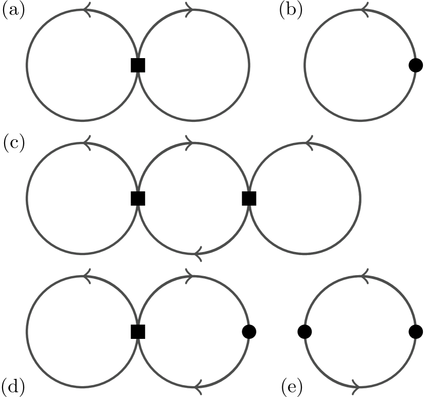
Figure 7: The connected integer time Feynman diagrams for the generating function of the CDA with interacting projectors defined in Eq. 184 at $\mathcal{N}=3$. Panels $a-e$ illustrate connected diagrams which appear in equations 188-192, respectively. Lines represent the non-interacting integer time Green’s function $\boldsymbol{g}_{0}$, squares represent the two-particle vertex associated with the variational parameter $u$, and circles represent the single-particle vertex associated with the variational parameter $\mu$.

V.2 Evaluating the SPD-l using the CDA

We now explore how to use the CDA in the context of the SPD-l. First recall that in Section III.2 we explored how to evaluate the SPD-l using a diagrammatic approach. Now we approach the same problem using the generating function and the CDA. Starting from the sequential discrete action of the SPD-l, we can trace out all of the orbitals that are not in the space of the interacting projector, which we denote as bath orbitals, and obtain a local discrete action as

$$\textrm{\@text@baccent{$\hat{\spdsymb}$}}_{loc} =\textrm{Tr}_{bath}\textrm{\@text@baccent{$\hat{\spdsymb}$}}=\textrm{Tr}_{bath}(\textrm{\@text@baccent{$\hat{\spdsymb}$}}_{0})\textrm{\@text@baccent{$\hat{P}$}}_{1}^{(1)}\dots\textrm{\@text@baccent{$\hat{P}$}}_{\mathcal{N}}^{(\mathcal{N})}$$ (193)

$$=\hat{\rho}_{G}(\boldsymbol{g}_{loc;0})\textrm{\@text@baccent{$\hat{P}$}}_{1}^{(1)}\dots\textrm{\@text@baccent{$\hat{P}$}}_{\mathcal{N}}^{(\mathcal{N})},$$ (194)

and we see that $\textrm{\@text@baccent{$\hat{\spdsymb}$}}_{loc}$ is indeed a CDA. If we study the generating function of the SPD-l, we find

$$Z(\boldsymbol{g}_{0})=\langle\textrm{\@text@baccent{$\hat{P}$}}\rangle_{\hat{\rho}_{G}(\boldsymbol{g}_{0})}=\langle\textrm{\@text@baccent{$\hat{P}$}}\rangle_{\hat{\rho}_{G}(\boldsymbol{g}_{loc;0})}=Z_{c}\left(\boldsymbol{g}_{loc;0}\right),$$ (195)

where $Z_{c}$ is the generating function of the CDA, the interacting projector is $\textrm{\@text@baccent{$\hat{P}$}}=\textrm{\@text@baccent{$\hat{P}$}}_{1}^{(1)}\dots\textrm{\@text@baccent{$\hat{P}$}}_{\mathcal{N}}^{(\mathcal{N})}$, and $\boldsymbol{g}_{loc;0}$ is the local impurity sub-block of the noninteracting integer time Green’s function, given as

$$\boldsymbol{g}_{0}=\left(\begin{array}[]{cc}\boldsymbol{g}_{loc;0}&\bm{g}_{lb;0}\\ \bm{g}_{bl;0}&\bm{g}_{bath;0}\end{array}\right),$$ (196)

and the latter equality in Eq. 195 holds given that $̱\hat{P}$ is local. Therefore, we can see that evaluating the SPD-l amounts to evaluating a CDA with the corresponding interacting projectors and a non-interacting integer time Green’s function $\boldsymbol{g}_{loc;0}$. It is useful to note that the integer time self-energy of the SPD-l is local

$$\boldsymbol{\Sigma}\left(\bm{g}_{0}\right)=\bm{\Sigma}_{loc}\left(\bm{g}_{loc;0}\right)\oplus\bm{0},$$ (197)

where $\bm{\Sigma}_{loc}$ is completely determined from $Z_{c}$, and this implies that

$$\bm{S}=\bm{S}_{loc}\oplus\boldsymbol{1}.$$ (198)

In summary, we have shown that by tracing out the bath orbitals of the SPD-l, one obtains a CDA which can be used to evaluate the SPD-l. In analogy to the traditional many-body Green’s function approach, the CDA is analogous to the action obtained by integrating out all bath states from the AIM. More precisely, for the particular case of the Trotter SPD-l in the large $\mathcal{N}$ limit, the Trotter SPD-l yields the exact density matrix of the corresponding Anderson impurity model, and the corresponding CDA is equivalent to the effective action of the impurity obtained by integrating out the bath sites.

VI Self-consistent Canonical Discrete Action (SCDA)

VI.1 Defining the SCDA algorithm

In the preceding sections, we have built a complete formalism for evaluating integer time correlation functions under a discrete action, which can then be used to evaluate an SPD. For a general SPD, one is still faced with a formidable problem, and therefore we need to develop approximations and search for relevant scenarios where an appropriate SPD can be exactly evaluated. Fortunately, all of the usual approaches from many-body physics can be generalized to our discrete action formalism.

A common scenario for models of interacting electrons is where the interaction is local, but not restricted to a single subspace; prominent examples include the Hubbard model and the periodic Anderson impurity model. In such cases, it is natural to study the SPD-d (see Section II), where the interacting projectors are composed of disjoint projectors. To specifically address the SPD-d, we introduce the self-consistent canonical discrete action approximation (SCDA), which is the integer time analogue of the dynamical mean-field theory (DMFT)[21, 22, 23]. The key idea for the SCDA is that the integer time self-energy is local, and this can be determined by mapping the SPD-d to a collection of CDA’s determined from a self-consistency condition. Analogous to DMFT, we will prove that the SCDA is an exact evaluation of the SPD-d in infinite dimensions (see Section VI.2).

We begin by outlining the SCDA in the most general case, in the absence of any symmetry, where we consider an SPD-d with $N$ sites and the interacting projectors are local within each site. The key idea for the SCDA is the assumption that the integer time self-energy is local

$$\bm{\Sigma}\left(\bm{g}\right)=\oplus_{i=1}^{N}\boldsymbol{\Sigma}_{i}(\boldsymbol{g}_{ii}),$$ (199)

where $i$ labels a given site. The self-consistent procedure can then be defined, beginning with an initial guess for the non-interacting integer time Green’s function of the CDA and the identification of the interacting projector of the CDA as that from site $i$ of the SPD-d, and we have

$$\bm{\mathcal{G}}_{i} =\boldsymbol{g}_{0;ii}, \textrm{\@text@baccent{$\hat{P}$}}_{i}=\prod_{\tau=1}^{\mathcal{N}}\textrm{\@text@baccent{$\hat{P}$}}_{i,\tau}^{(\tau)},$$ (200)

which completely defines the effective CDA for site $i$. The effective CDA can then be solved by computing the discrete generating function $Z_{i}$, yielding the exponential integer time self-energy $\boldsymbol{S}_{i}$ as

$$\boldsymbol{S}_{i}=\left(Z_{i}\boldsymbol{1}+\frac{\partial Z_{i}}{\partial\boldsymbol{\mathcal{G}}_{i}^{T}}(\boldsymbol{1}-\bm{\mathcal{G}}_{i})\right)^{-1}\left(Z_{i}\boldsymbol{1}-\frac{\partial Z_{i}}{\partial\boldsymbol{\mathcal{G}}_{i}^{T}}\bm{\mathcal{G}}_{i}\right).$$ (201)

In the absence of symmetry, one must solve a CDA for each site, yielding the total exponential self-energy for the system as

$$\boldsymbol{S}=\oplus_{i=1}^{N}\boldsymbol{S}_{i}.$$ (202)

The interacting integer time Green’s function can then be constructed as

$$\bm{g}=\frac{\boldsymbol{1}}{\boldsymbol{g}_{0}+\left(\boldsymbol{1}-\bm{g}_{0}\right)\bm{S}}\bm{g}_{0}.$$ (203)

Finally, we construct a new non-interacting integer time Green’s function, yielding the updated CDA

$$\bm{\mathcal{G}}_{i}=\bm{S}_{i}\frac{\boldsymbol{1}}{\left(\boldsymbol{1}+\bm{g}{}_{ii}\left(\bm{S}_{i}-\boldsymbol{1}\right)\right)}\bm{g}{}_{ii}.$$ (204)

This entire procedure is then iterated until self-consistency is achieved. Upon achieving self-consistency, one has completed a single evaluation of the SPD-d. In order to obtain the ground state energy, one needs to minimize over the variational parameters.

The preceding outline of the SCDA is applied to a generic system without symmetry, and now we specify the SCDA to the case of translation symmetry where all types of orbitals have the same density-of-states. We can begin with a guess for the non-interacting integer time impurity Green’s function $\bm{\mathcal{G}}$ as

$$\bm{\mathcal{G}}=\int d\epsilon D\left(\epsilon\right)\bm{g}_{0}\left(\epsilon\right),$$ (205)

where $D(\epsilon)$ is the density-of-states. This defines our effective CDA for the crystal, which can then be solved by computing the discrete generating function $Z$, yielding the local exponential integer time self-energy $\boldsymbol{S}$ as

$$\boldsymbol{S}_{loc}=\left(Z\boldsymbol{1}+\frac{\partial Z}{\partial\boldsymbol{\mathcal{G}}^{T}}(\boldsymbol{1}-\bm{\mathcal{G}})\right)^{-1}\left(Z\boldsymbol{1}-\frac{\partial Z}{\partial\boldsymbol{\mathcal{G}}^{T}}\bm{\mathcal{G}}\right).$$ (206)

We then use this integer time self-energy to update the interacting integer time Green’s function for each energy orbital as

$$\bm{g}\left(\epsilon\right)=\frac{\boldsymbol{1}}{\boldsymbol{g}_{0}\left(\epsilon\right)+\left(\boldsymbol{1}-\bm{g}_{0}\left(\epsilon\right)\right)\bm{S}_{loc}}\bm{g}_{0}\left(\epsilon\right).$$ (207)

Then we obtain the new interacting local integer time Green’s function as

$$\bm{g}_{loc}=\int d\epsilon D\left(\epsilon\right)\bm{g}\left(\epsilon\right).$$ (208)

Finally, we construct a new non-interacting integer time Green’s function, yielding the updated CDA as

$$\bm{\mathcal{G}}=\bm{S}_{loc}\frac{\boldsymbol{1}}{\left(\boldsymbol{1}+\bm{g}_{loc}\left(\bm{S}_{loc}-\boldsymbol{1}\right)\right)}\bm{g}{}_{loc}.$$ (209)

This process is then iterated until self-consistency is achieved, and then the entire procedure is iterated when minimizing over the variational parameters (see Figure 8).

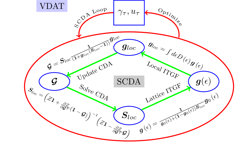
Figure 8: A schematic of how VDAT is used to solve for the ground state properties of a Hamiltonian under SPD-d within the SCDA. ITGF is the acronym for the integer time Green’s function.

VI.2 Proof that the SCDA is exact in $d=\infty$

Here we prove that the SCDA exactly evaluates the SPD-d in $d=\infty$ for a general multi-band Hubbard model, where the local interacting projectors $\hat{P}_{i}$ are confined to site $i$. The main idea follows the cavity construction method used for proving that DMFT is exact in infinite dimensions[21]. We begin by considering the non-interacting discrete action

$$\textrm{\@text@baccent{$\hat{\spdsymb}$}}_{0}=\textrm{\@text@baccent{$\hat{Q}$}}\exp(\bm{\gamma}_{1}\cdot\textrm{\@text@baccent{$\hat{\bm{n}}$}}^{(1)})...\exp(\bm{\gamma}_{\mathcal{N}}\cdot\textrm{\@text@baccent{$\hat{\bm{n}}$}}^{(\mathcal{N})}),$$ (210)

where

$$\exp(\bm{\gamma}_{\tau}\cdot\textrm{\@text@baccent{$\hat{\bm{n}}$}}^{(\tau)})=\exp(\sum_{\mathbf{k}\sigma}\gamma_{\mathbf{k}\sigma;\tau}\textrm{\@text@baccent{$\hat{n}$}}_{\mathbf{k}\sigma}^{(\tau)}),$$ (211)

In the cavity construction, one selects a particular site in the lattice, denoted site $i$, and traces out all other sites. We can rewrite the non-interacting discrete action in the following form

$$\textrm{\@text@baccent{$\hat{\spdsymb}$}}_{0}=\exp\left(\left(\bm{v}_{i}+\bm{v}_{b}+\bm{v}_{ib}\right)\cdot\textrm{\@text@baccent{$\hat{\bm{n}}$}}\right),$$ (212)

where $\boldsymbol{v}_{i}$ is a single-particle potential within site $i$, $\boldsymbol{v}_{b}$ is the single-particle potential of the remaining sites, and $\boldsymbol{v}_{ib}$ is the off-diagonal component of the single-particle potential between site $i$ and the remaining sites. We can then construct the local discrete action for site $i$ by tracing out all other sites

$$\textrm{\@text@baccent{$\hat{\spdsymb}$}}_{loc} =\text{Tr}_{/i}\bigg{(}\textrm{\@text@baccent{$\hat{\spdsymb}$}}_{0}\prod_{j}\textrm{\@text@baccent{$\hat{P}$}}_{j}\bigg{)}=\textrm{\@text@baccent{$\hat{\spdsymb}$}}_{loc;0}\textrm{\@text@baccent{$\hat{P}$}}_{i},$$ (213)

where

$$\textrm{\@text@baccent{$\hat{\spdsymb}$}}_{loc;0} =\text{Tr}_{/i}\bigg{(}\textrm{\@text@baccent{$\hat{\spdsymb}$}}_{0}\prod_{j\neq i}\textrm{\@text@baccent{$\hat{P}$}}_{j}\bigg{)}, \textrm{\@text@baccent{$\hat{P}$}}_{j}=\prod_{\tau=1}^{\mathcal{N}}\textrm{\@text@baccent{$\hat{P}$}}_{\tau,j}^{(\tau)}.$$ (214)

We now seek to prove that $\textrm{\@text@baccent{$\hat{\spdsymb}$}}_{loc}$ is a CDA in $d=\infty$. By expanding $\textrm{\@text@baccent{$\hat{\spdsymb}$}}_{loc;0}$ in terms of $\boldsymbol{v}_{ib}$, we prove that the interacting projectors within $\textrm{\@text@baccent{$\hat{\spdsymb}$}}_{loc;0}$ can be replaced by an effective non-interacting projector as

$$\textrm{\@text@baccent{$\hat{\spdsymb}$}}_{loc;0} =\text{Tr}_{/i}(\textrm{\@text@baccent{$\hat{\spdsymb}$}}_{0}\exp(\boldsymbol{\Sigma}_{B;i}\textrm{\@text@baccent{$\hat{\bm{n}}$}})),$$ (215)

where $\boldsymbol{\Sigma}_{B;i}$ is a single-particle potential for the sites not containing $i$. Recall the general expression for the expansion of the exponential of a sum of two operators $̱\hat{A}$ and $̱\hat{B}$

$$\exp(\textrm{\@text@baccent{$\hat{A}$}}+\textrm{\@text@baccent{$\hat{B}$}})=\exp(\textrm{\@text@baccent{$\hat{A}$}})+$$

$$\int_{0}^{1}d\lambda\exp(\lambda\textrm{\@text@baccent{$\hat{A}$}})\textrm{\@text@baccent{$\hat{B}$}}\exp((1-\lambda)\textrm{\@text@baccent{$\hat{A}$}})+$$

$$\int_{0}^{1}d\lambda_{1}\int_{\lambda_{1}}^{1}d\lambda_{2}\exp(\lambda_{1}\textrm{\@text@baccent{$\hat{A}$}})\textrm{\@text@baccent{$\hat{B}$}}\exp((\lambda_{2}-\lambda_{1})\textrm{\@text@baccent{$\hat{A}$}})\textrm{\@text@baccent{$\hat{B}$}}\times$$

$$\exp((1-\lambda_{2})\textrm{\@text@baccent{$\hat{A}$}})+\dots$$ (216)

and equating

$̱\hat{A}$ $$=(\bm{v}_{i}+\bm{v}_{b})\cdot\textrm{\@text@baccent{$\hat{\bm{n}}$}}=\textrm{\@text@baccent{$\hat{A}$}}_{i}+\textrm{\@text@baccent{$\hat{A}$}}_{b},$$ (217)

$$\textrm{\@text@baccent{$\hat{A}$}}_{i} =\bm{v}_{i}\cdot\textrm{\@text@baccent{$\hat{\bm{n}}$}}=\sum_{\tau\tau^{\prime}}v^{\tau\tau^{\prime}}\textrm{\@text@baccent{$\hat{a}$}}_{i}^{\dagger\left(\tau\right)}\textrm{\@text@baccent{$\hat{a}$}}_{i}^{\left(\tau^{\prime}\right)}+h.c.,$$ (218)

$$\textrm{\@text@baccent{$\hat{A}$}}_{b} =\bm{v}_{b}\cdot\textrm{\@text@baccent{$\hat{\bm{n}}$}}=\sum_{j\neq i,j^{\prime}\neq i,\tau\tau^{\prime}}v_{jj^{\prime}}^{\tau\tau^{\prime}}\textrm{\@text@baccent{$\hat{a}$}}_{j}^{\dagger\left(\tau\right)}\textrm{\@text@baccent{$\hat{a}$}}_{j^{\prime}}^{\left(\tau^{\prime}\right)},$$ (219)

$̱\hat{B}$ $$=\bm{v}_{ib}\cdot\textrm{\@text@baccent{$\hat{\bm{n}}$}}=\sum_{j\neq i,\tau\tau^{\prime}}(t_{j}^{\tau\tau^{\prime}}\textrm{\@text@baccent{$\hat{a}$}}_{i}^{\dagger\left(\tau\right)}\textrm{\@text@baccent{$\hat{a}$}}_{j}^{\left(\tau^{\prime}\right)}+h.c.),$$ (220)

we can then consider the expansion in $\boldsymbol{v}_{ib}$ order by order

$$\hat{\rho}_{loc;0}=\text{Tr}_{/i}\bigg{(}\exp(\textrm{\@text@baccent{$\hat{A}$}})\prod_{j\neq i}\hat{P}_{j}\bigg{)}+\left[\hat{\rho}_{loc;0}\right]_{1}+\dots$$ (221)

where

$$\left[\textrm{\@text@baccent{$\hat{\spdsymb}$}}_{loc;0}\right]_{1} =\text{Tr}_{/i}\left(\int_{0}^{1}d\lambda_{1}\exp(\lambda_{1}\textrm{\@text@baccent{$\hat{A}$}})\sum_{j_{1}\neq i,\tau\tau^{\prime}}\left(t_{j_{1}}^{\tau\tau^{\prime}}\textrm{\@text@baccent{$\hat{a}$}}_{i}^{\dagger\left(\tau\right)}\textrm{\@text@baccent{$\hat{a}$}}_{j_{1}}^{\left(\tau^{\prime}\right)}+h.c.\right)\exp((1-\lambda_{1})\textrm{\@text@baccent{$\hat{A}$}})\prod_{j\neq i}\textrm{\@text@baccent{$\hat{P}$}}_{j}\right),$$ (222)

$$\left[\textrm{\@text@baccent{$\hat{\spdsymb}$}}_{loc;0}\right]_{2} =\text{Tr}_{/i}\bigg{(}\int_{0}^{1}d\lambda_{1}\int_{\lambda_{1}}^{1}d\lambda_{2}\exp(\lambda_{1}\textrm{\@text@baccent{$\hat{A}$}})\sum_{j_{1}\neq i,\tau_{1}\tau_{1}^{\prime}}\left(t_{j_{1}}^{\tau_{1}\tau_{1}^{\prime}}\textrm{\@text@baccent{$\hat{a}$}}_{i}^{\dagger\left(\tau_{1}\right)}\textrm{\@text@baccent{$\hat{a}$}}_{j_{1}}^{\left(\tau_{1}^{\prime}\right)}+h.c.\right)\exp((\lambda_{2}-\lambda_{1})\textrm{\@text@baccent{$\hat{A}$}})$$

$$\times\sum_{j_{2}\neq i,\tau_{2}\tau_{2}^{\prime}}\left(t_{j_{2}}^{\tau_{2}\tau_{2}^{\prime}}\textrm{\@text@baccent{$\hat{a}$}}_{i}^{\dagger\left(\tau_{2}\right)}\textrm{\@text@baccent{$\hat{a}$}}_{j_{2}}^{\left(\tau_{2}^{\prime}\right)}+h.c.\right)\exp((1-\lambda_{2})\textrm{\@text@baccent{$\hat{A}$}})\prod_{j\neq i}\textrm{\@text@baccent{$\hat{P}$}}_{j}\bigg{)}.$$ (223)

We observe that a cavity Green’s function emerges as a key quantity to evaluate

$$G_{j_{1}j_{2}}^{\tau_{1}\tau_{2}}(\lambda_{1},\lambda_{2})=\text{Tr}_{/i}\bigg{(}\exp(\lambda_{1}\textrm{\@text@baccent{$\hat{A}$}}_{b})\textrm{\@text@baccent{$\hat{a}$}}_{j_{1}}^{\left(\tau_{1}\right)}\times$$

$$\exp((\lambda_{2}-\lambda_{1})\textrm{\@text@baccent{$\hat{A}$}}_{b})\textrm{\@text@baccent{$\hat{a}$}}_{j_{2}}^{\dagger\left(\tau_{2}\right)}\exp((1-\lambda_{2})\textrm{\@text@baccent{$\hat{A}$}}_{b})\prod_{j\neq i}\textrm{\@text@baccent{$\hat{P}$}}_{j}\bigg{)}.$$ (224)

Given that the projectors $\textrm{\@text@baccent{$\hat{P}$}}_{j}$ are local, the scaling of the cavity Green’s function is[21]

$$G_{j_{1}j_{2}}^{\tau_{1}\tau_{2}}(\lambda_{1},\lambda_{2}) \sim\left(\frac{1}{\sqrt{d}}\right)^{\left|j-j^{\prime}\right|},$$ (225)

where $d$ is the dimension of the lattice. Analogous to the case of DMFT, the local discrete action $\textrm{\@text@baccent{$\hat{\spdsymb}$}}_{loc;0}$ only depends on $G_{j_{1}j_{2}}^{\tau_{1}\tau_{2}}(0,0)$ and $\textrm{\@text@baccent{$\hat{A}$}}_{b}$. To illustrate this, consider the second order contribution

$$\text{Tr}_{/i}\bigg{(} \exp(\lambda_{1}\textrm{\@text@baccent{$\hat{A}$}})t_{j_{1}}^{\tau_{1}\tau_{1}^{\prime}}\textrm{\@text@baccent{$\hat{a}$}}_{i}^{\dagger\left(\tau_{1}\right)}\textrm{\@text@baccent{$\hat{a}$}}_{j_{1}}^{\left(\tau_{1}^{\prime}\right)}\exp((\lambda_{2}-\lambda_{1})\textrm{\@text@baccent{$\hat{A}$}})\times$$

$$t_{j_{2}}^{\tau_{2}\tau_{2}^{\prime}}\textrm{\@text@baccent{$\hat{a}$}}_{j_{2}}^{\dagger\left(\tau_{2}\right)}\textrm{\@text@baccent{$\hat{a}$}}_{i}^{\left(\tau_{2}^{\prime}\right)}\exp((1-\lambda_{2})\textrm{\@text@baccent{$\hat{A}$}})\prod_{j\neq i}\textrm{\@text@baccent{$\hat{P}$}}_{j}\bigg{)}$$

$$= t_{j_{1}}^{\tau_{1}\tau_{1}^{\prime}}t_{j_{2}}^{\tau_{2}\tau_{2}^{\prime}}G_{j_{1}j_{2}}^{\tau_{1}^{\prime}\tau_{2}}(\lambda_{1},\lambda_{2})\exp(\lambda_{1}\textrm{\@text@baccent{$\hat{A}$}}_{i})\textrm{\@text@baccent{$\hat{a}$}}_{i}^{\dagger\left(\tau_{1}\right)}\times$$

$$\exp((\lambda_{2}-\lambda_{1})\textrm{\@text@baccent{$\hat{A}$}}_{i})\textrm{\@text@baccent{$\hat{a}$}}_{i}^{\left(\tau_{2}^{\prime}\right)}\exp((1-\lambda_{2})\textrm{\@text@baccent{$\hat{A}$}}_{i}),$$ (226)

where the Einstein summation convention is assumed for the orbital and time index. The total scaling of this term will be

$$d^{|j_{1}-i|}d^{|j_{2}-i|}d^{-\frac{1}{2}|j_{1}-i|}d^{-\frac{1}{2}|j_{2}-i|}d^{-\frac{1}{2}|j_{1}-j_{2}|}\sim 1.$$ (227)

Considering a fourth order contribution

$$t_{j_{1}}^{\tau_{1}\tau_{1}^{\prime}}t_{j_{2}}^{\tau_{2}\tau_{2}^{\prime}}t_{j_{3}}^{\tau_{3}\tau_{3}^{\prime}}t_{j_{4}}^{\tau_{4}\tau_{4}^{\prime}}G_{j_{1}j_{2}j_{3}j_{4}}^{\tau_{1}^{\prime}\tau_{2}\tau_{3}^{\prime}\tau_{4}}(\lambda_{1},\lambda_{2},\lambda_{3},\lambda_{4})\exp(\lambda_{1}\textrm{\@text@baccent{$\hat{A}$}}_{i})\times$$

$$a_{i}^{\dagger\left(\tau_{1}\right)}\exp((\lambda_{2}-\lambda_{1})\textrm{\@text@baccent{$\hat{A}$}}_{i})a_{i}^{\left(\tau_{2}^{\prime}\right)}\exp((\lambda_{3}-\lambda_{2})\textrm{\@text@baccent{$\hat{A}$}}_{i})\times$$

$$a_{i}^{\dagger\left(\tau_{3}\right)}\exp((\lambda_{4}-\lambda_{3})\textrm{\@text@baccent{$\hat{A}$}}_{i})a_{i}^{\left(\tau_{4}^{\prime}\right)}\exp((1-\lambda_{4})\textrm{\@text@baccent{$\hat{A}$}}_{i}),$$ (228)

the scaling for one of the connected portions is

$$d^{|j_{1}-i|}d^{|j_{2}-i|}d^{|j_{3}-i|}d^{|j_{4}-i|}d^{-\frac{1}{2}|j_{1}-i|}d^{-\frac{1}{2}|j_{2}-i|}\times$$

$$d^{-\frac{1}{2}|j_{3}-i|}d^{-\frac{1}{2}|j_{4}-i|}d^{-\frac{1}{2}|j_{1}-j_{2}|}d^{-\frac{1}{2}|j_{2}-j_{3}|}d^{-\frac{1}{2}|j_{3}-j_{4}|}$$ (229)

$$\sim d^{-\frac{1}{2}|j_{2}-j_{3}|}\rightarrow 0,$$ (230)

and all other connected diagrams will scale to zero as well. The same result holds for higher orders, thus proving Eq. 215.

We proceed by rewriting $\textrm{\@text@baccent{$\hat{\spdsymb}$}}_{loc;0}$ as

$$\textrm{\@text@baccent{$\hat{\spdsymb}$}}_{loc;0}=\text{Tr}_{/i}\left(\textrm{\@text@baccent{$\hat{\spdsymb}$}}^{\star}\exp\left(-\boldsymbol{\Sigma}_{loc;i}\cdot\textrm{\@text@baccent{$\hat{\bm{n}}$}}\right)\right),$$ (231)

$$\textrm{\@text@baccent{$\hat{\spdsymb}$}}^{\star}=\textrm{\@text@baccent{$\hat{\spdsymb}$}}_{0}\exp\left(\left(\boldsymbol{\Sigma}_{B;i}+\boldsymbol{\Sigma}_{loc;i}\right)\cdot\textrm{\@text@baccent{$\hat{\bm{n}}$}}\right),$$ (232)

where $\boldsymbol{\Sigma}_{loc;i}$ is the integer time self-energy for the CDA with a given $\textrm{\@text@baccent{$\hat{\spdsymb}$}}_{loc;0}$ and thus is a single-particle potential within the site $i$; and $\textrm{\@text@baccent{$\hat{\spdsymb}$}}^{\star}$ is a non-interacting discrete action that has the same integer time Green’s function as $̱\hat{\varrho}$. It should be noted that $\boldsymbol{\Sigma}_{loc;i}$ and $\boldsymbol{\Sigma}_{B;i}$ occupy distinct blocks within the integer time self-energy matrix and do not mix.

Finally, we prove that $\boldsymbol{\Sigma}$ is the sum of the local integer time self-energy for all sites. To see this, we notice that the above construction can be applied to every site $i$, and thus we have $\boldsymbol{\Sigma}=\boldsymbol{\Sigma}_{B;i}+\boldsymbol{\Sigma}_{loc;i}$ for every site $i$. Recalling the block structure of the self-energy, we can solve for $\boldsymbol{\Sigma}=\sum_{i}\boldsymbol{\Sigma}_{loc;i}$ , proving the SCDA self-consistency condition, analogous to DMFT.

For the special case of $\mathcal{N}=2$ with a G-type SPD-d, the SCDA recovers the classic observation that the Gutzwiller approximation exactly evaluates the Gutzwiller wave function in $d=\infty$ [14, 15, 16, 17]. For $\mathcal{N}=2$ with a B-type SPD-d, our proof demonstrates that the Baeriswyl wave function[41] is exactly evaluated in $d=\infty$ via the SCDA, which was not previously known. For the case of $\mathcal{N}=3$, we see that the Gutzwiller-Baeriswyl[18] and Baeriswyl-Gutzwiller[19] wave functions can be exactly evaluated in $d=\infty$, which also was not known. Furthermore, there are an infinite number of wave functions for $\mathcal{N}\geq 4$ which have not been considered, but can be exactly evaluated via the SCDA.

VI.3 The SCDA for $\mathcal{N}=2$

Here we consider the case of $\mathcal{N}=2$ for the Hubbard model, which is of practical importance given that it recovers the Gutzwiller approximation. We will demonstrate that the SCDA at $\mathcal{N}=2$ is a very special case in that the SCDA self-consistency condition can be achieved a priori by choosing $\boldsymbol{\mathcal{G}}$ as the non-interacting local integer time Green’s function and constraining the interacting projector such that $\hat{\varrho}_{loc}$ and $\hat{\varrho}_{loc;0}$ have the same local single-particle density matrix. Given this particular implementation of the SCDA at $\mathcal{N}=2$, we can explicitly derive the Gutzwiller equations. Alternatively, we could choose not follow such constraints, and then the SCDA self-consistency condition cannot be fulfulled a priori, though we are gauranteed to reach the same ground state properties. This latter scenario could be numerically beneficial given that we will not need to satisfy any constraint when minimizing over the variational parameters, though we will need to execute the SCDA self-consistency condition instead.

In the remainder of this subsection, we will explicitly derive the Gutzwiller equations in a sequence of increasingly complex scenarios: the single-band Hubbard model at half-filling, the multi-band Hubbard model at arbitrary filling but with symmtery dictating that the local single-particle density matrix is diagonal, and finally the most general possible case for the multi-band Hubbard model. The last case results in rotationally invariant Gutzwiller equations in an arbitrary basis, which have not yet been presented in the literature; and they recover the particular case of a “mixed original-natural basis”[49].

VI.3.1 Single-band Hubbard model at half-filling

To understand how the SCDA works, we study the case of $\mathcal{N}=2$ for a G-type SPD-d, which recovers the Gutzwiller approximation. We first focus on the case of the one band model at half-filling, and we later generalize to the multi-orbital case at arbitrary density. For the former, the SPD-d is

$$\hat{\varrho}=\exp(\sum_{i}u\Delta\hat{d}_{i})\exp(\sum_{\epsilon\sigma}\gamma_{\sigma}(\epsilon)\hat{n}_{\epsilon\sigma})\exp(\sum_{i}u\Delta\hat{d}_{i}),$$ (233)

where $\Delta\hat{d}$ is defined in Eq. 36, $\hat{n}_{\epsilon\sigma}$ is the number operator for the orbital with energy $\epsilon$ and spin $\sigma$, and the variational parameters are $u$ and $\gamma_{\sigma}(\epsilon)$. Thus, the non-interacting integer time Green’s function for spin $\sigma$ and energy $\epsilon$ is

$$\bm{g}_{0;\sigma}(\epsilon)=\begin{pmatrix}n_{\sigma}(\epsilon)&\left(1-n_{\sigma}(\epsilon)\right)\\ -n_{\sigma}(\epsilon)&n_{\sigma}(\epsilon)\end{pmatrix},$$ (234)

where

$$n_{\sigma}(\epsilon)=\frac{1}{1+\exp\left(-\gamma_{\sigma}(\epsilon)\right)}\in[0,1],$$ (235)

is used as a reparameterization of the variational parameter $\gamma_{\sigma}(\epsilon)$. As an initial guess, we choose the non-interacting integer time Green’s function of the CDA as the local non-interacting integer time Green’s function, given as

$$\boldsymbol{\mathcal{G}}_{\sigma}=\int d\epsilon D(\epsilon)\bm{g}_{0;\sigma}(\epsilon)=\begin{pmatrix}\frac{1}{2}&\frac{1}{2}\\ -\frac{1}{2}&\frac{1}{2}\end{pmatrix},$$ (236)

where $D(\epsilon)$ is the density-of-states per spin. It will also be necessary to introduce $\boldsymbol{\mathcal{G}}$ for an arbitrary density and spin as

$$\boldsymbol{\mathcal{G}}=\left(\begin{array}[]{cccc}a_{11\uparrow}&0&a_{12\uparrow}&0\\ 0&a_{11\downarrow}&0&a_{12\downarrow}\\ a_{21\uparrow}&0&a_{22\uparrow}&0\\ 0&a_{21\downarrow}&0&a_{22\downarrow}\end{array}\right),$$ (237)

where we have used the time major scheme (see Subsection III.2.1 for a definition), and this more general definition is needed given that we will take the derivative of the discrete generating function. The discrete generating function is given as

$$Z =1+\frac{1}{16}(uZ_{1}+u^{2}Z_{2}),$$ (238)

where

$$Z_{1}=8\left(\left(2a_{22\downarrow}-1\right)a_{22\uparrow}-a_{22\downarrow}\right)+$$

$$16a_{11\downarrow}a_{11\uparrow}-8a_{11\downarrow}-8a_{11\uparrow}+8,$$ (239)

and

$$Z_{2}=4a_{12\downarrow}a_{21\downarrow}\left(4a_{12\uparrow}a_{21\uparrow}+2a_{22\uparrow}-1\right)+1+$$

$$2\left(\left(2a_{22\downarrow}-1\right)a_{22\uparrow}-a_{22\downarrow}\right)-4a_{22\downarrow}a_{11\uparrow}\left(2a_{22\uparrow}-1\right)+$$

$$4a_{11\downarrow}\left(2\left(1-2a_{22\downarrow}\right)a_{12\uparrow}a_{21\uparrow}+a_{22\downarrow}\left(1-2a_{22\uparrow}\right)\right)+$$

$$4a_{11\downarrow}\left(a_{22\uparrow}-2a_{11\uparrow}a_{22\uparrow}+2a_{22\downarrow}a_{11\uparrow}\left(2a_{22\uparrow}-1\right)\right)+$$

$$4\left(2a_{22\downarrow}-1\right)a_{12\uparrow}a_{21\uparrow}-8a_{12\downarrow}a_{21\downarrow}a_{11\uparrow}\left(2a_{22\uparrow}-1\right)+$$

$$a_{11\downarrow}\left(4a_{11\uparrow}-2\right)-2a_{11\uparrow}+4a_{11\uparrow}a_{22\uparrow}.$$ (240)

Evaluating $Z$ and its derivatives for half filling gives

$$Z=\frac{u^{2}}{16}+1, \frac{\partial Z}{\partial\boldsymbol{\mathcal{G}}_{\sigma}^{T}}=\left(\begin{array}[]{cc}0&-\frac{u^{2}}{8}\\ \frac{u^{2}}{8}&0\end{array}\right),$$ (243)

and using the discrete Dyson equation, we have

$$\boldsymbol{g}_{\sigma} =\boldsymbol{\mathcal{G}}_{\sigma}+\frac{1}{Z}(\boldsymbol{1}-\boldsymbol{\mathcal{G}}_{\sigma})\frac{\partial Z}{\partial\boldsymbol{\mathcal{G}}_{\sigma}^{T}}\boldsymbol{\mathcal{G}}_{\sigma}$$ (244)

$$=\left(\begin{array}[]{cc}\frac{1}{2}&\frac{1}{2}z(u)\\ -\frac{1}{2}z(u)&\frac{1}{2}\end{array}\right),$$ (247)

where

$$z(u)=\frac{32}{u^{2}+16}-1.$$ (248)

The exponential integer time self-energy can be constructed as

$$S_{\sigma} =\left(Z+\frac{\partial Z}{\partial\boldsymbol{\mathcal{G}}_{\sigma}^{T}}(1-\boldsymbol{\mathcal{G}}_{\sigma})\right)^{-1}\left(Z-\frac{\partial Z}{\partial\boldsymbol{\mathcal{G}}_{\sigma}^{T}}\boldsymbol{\mathcal{G}}_{\sigma}\right)$$ (249)

$$=\left(\begin{array}[]{cc}\frac{512}{u^{4}+256}-1&\frac{32u^{2}}{u^{4}+256}\\ -\frac{32u^{2}}{u^{4}+256}&\frac{512}{u^{4}+256}-1\end{array}\right)$$ (252)

$$=\left(\begin{array}[]{cc}\frac{2z(u)}{z(u)^{2}+1}&\frac{2}{z(u)^{2}+1}-1\\ 1-\frac{2}{z(u)^{2}+1}&\frac{2z(u)}{z(u)^{2}+1}\end{array}\right).$$ (255)

The interacting integer time Green’s function for a given $\epsilon\sigma$ is then

$$\bm{g}_{\sigma}(\epsilon)=\begin{pmatrix}n_{\sigma}(\epsilon)&\left(1-n_{\sigma}(\epsilon)\right)z(u)\\ -n_{\sigma}(\epsilon)z(u)&\left(n_{\sigma}(\epsilon)-\frac{1}{2}\right)z(u)^{2}+\frac{1}{2}\end{pmatrix}.$$ (256)

The new interacting local integer time Green’s function can then be constructed as

$$\bm{g}^{\prime}_{loc;\sigma}=\int d\epsilon D\left(\epsilon\right)\bm{g}_{\sigma}(\epsilon)=\begin{pmatrix}\frac{1}{2}&\frac{1}{2}z(u)\\ -\frac{1}{2}z(u)&\frac{1}{2}\end{pmatrix},$$ (257)

which is same as the interacting local integer time Green’s function from the initial guess. Therefore, we have already achieved self-consistency. In order to evaluate the ground state energy, we also need to evaluate the double occupancy as

$$\langle\Delta\hat{d}\rangle_{\hat{\varrho}} =\frac{2u}{u^{2}+16}\equiv\Delta d,$$ (258)

which is computed by evaluating Eq. 173. Now we can proceed to minimize over the variational parameters

$$\mathcal{E} =\min_{u,n_{\epsilon\sigma}\in\left[0,1\right]}\left(\frac{2uU}{u^{2}+16}+\sum_{\sigma}\int d\epsilon D(\epsilon)n_{\sigma}(\epsilon)z(u)^{2}\right)$$ (259)

$$=\min_{u}\left(\frac{2uU}{u^{2}+16}+\epsilon_{0}z(u)^{2}\right)$$ (260)

$$=\min_{\Delta d\in[-\frac{1}{4},\frac{1}{4}]}(\Delta dU+\epsilon_{0}(1-(4\Delta d)^{2}))$$ (261)

$$=\begin{cases}\epsilon_{0}-\frac{U^{2}}{64\epsilon_{0}}&U\leq 8\epsilon_{0}\\ 0&U\geq 8\epsilon_{0}\end{cases},$$ (262)

where $\epsilon_{0}=2\int_{-\infty}^{0}d\epsilon D(\epsilon)\epsilon$. Here we see that we have recovered the Gutzwiller approximation, with the Brinkman-Rice transition[50] at $U=8\epsilon_{0}$.

VI.3.2 Multi-band Hubbard model at arbitrary filling with a diagonal local single-particle density matrix

Here the preceding analysis is generalized to the multi-band Hubbard model for the special case where symmetry dictates that the local single-particle density matrix is diagonal, and we recover the usual Gutzwilller approximation in this scenario. We begin with the SPD for this multi-band case

$$\hat{\varrho}=\left(\prod_{i}\hat{P}_{1,i}\right)\exp(\sum_{\epsilon\alpha}\gamma_{\alpha}(\epsilon)\hat{n}_{\epsilon\alpha})\left(\prod_{i}\hat{P}_{2,i}\right),$$ (263)

where $\hat{P}_{1,i}=\sum_{\Gamma\Gamma^{\prime}}P_{1,\Gamma\Gamma^{\prime}}\hat{X}_{i;\Gamma\Gamma^{\prime}}=\hat{P}_{2,i}^{\dagger}$ is the interacting projector of site $i$ in the physical space, and the variational parameters are $P_{1,\Gamma\Gamma^{\prime}}$. The non-interacting integer time Green’s function for orbital $\epsilon\alpha$ is then

$$\bm{g}_{0;\alpha}(\epsilon)=\begin{pmatrix}n_{\alpha}(\epsilon)&\left(1-n_{\alpha}(\epsilon)\right)\\ -n_{\alpha}(\epsilon)&n_{\alpha}(\epsilon)\end{pmatrix},$$ (264)

where

$$n_{\alpha}(\epsilon)=\frac{1}{1+\exp\left(-\gamma_{\alpha}(\epsilon)\right)}\in[0,1]$$ (265)

is used as a reparameterization of the variational parameters $\gamma_{\alpha}(\epsilon)$. As an initial guess, we choose the non-interacting integer time Green’s function of the CDA to be the non-interacting local integer time Green’s function

$$\boldsymbol{\mathcal{G}}_{\alpha}=\int d\epsilon D_{\alpha}\left(\epsilon\right)\bm{g}_{0;\alpha}(\epsilon)=\begin{pmatrix}\bar{n}_{\alpha}&\left(1-\bar{n}_{\alpha}\right)\\ -\bar{n}_{\alpha}&\bar{n}_{\alpha}\end{pmatrix},$$ (266)

where $D_{\alpha}(\epsilon)$ is the partial density-of-states and $\bar{n}_{\alpha}=\int d\epsilon D_{\alpha}\left(\epsilon\right)n_{\alpha}(\epsilon)$. Considering the CDA of site $i$ for this SPD-d, we have

$$\textrm{\@text@baccent{$\hat{\spdsymb}$}}_{loc}=\textrm{\@text@baccent{$\hat{\spdsymb}$}}_{loc;0}\textrm{\@text@baccent{$\hat{P}$}}_{1,i}^{(1)}\textrm{\@text@baccent{$\hat{P}$}}_{2,i}^{(2)},$$ (267)

$$\textrm{\@text@baccent{$\hat{\spdsymb}$}}_{loc;0}=\hat{\rho}_{G}(\boldsymbol{\mathcal{G}})=\textrm{\@text@baccent{$\hat{Q}$}}\exp(\boldsymbol{v}_{1}\cdot\textrm{\@text@baccent{$\hat{\bm{n}}$}}_{i}^{(1)}+\boldsymbol{v}_{2}\cdot\textrm{\@text@baccent{$\hat{\bm{n}}$}}_{i}^{(2)}),$$ (268)

where

$$\boldsymbol{v}_{1} =0, [\boldsymbol{v}_{2}]_{\alpha,\alpha^{\prime}}=-\delta_{\alpha,\alpha^{\prime}}\ln(\bar{n}_{\alpha}^{-1}-1).$$ (269)

We see that $\textrm{\@text@baccent{$\hat{\spdsymb}$}}_{loc}$ is an effective discrete action of an SPD given as

$$\hat{\varrho}_{loc}=\exp(\boldsymbol{v}_{1}\cdot\hat{\bm{n}}_{i})\hat{P}_{1,i}\exp(\boldsymbol{v}_{2}\cdot\hat{\bm{n}}_{i})\hat{P}_{2,i},$$ (270)

and

$$\hat{\varrho}_{loc;0}=\exp(\boldsymbol{v}_{1}\cdot\hat{\bm{n}}_{i})\exp(\boldsymbol{v}_{2}\cdot\hat{\bm{n}}_{i}).$$ (271)

We can now directly evaluate the interacting integer time Green’s function as

$$\bm{g}_{loc;\alpha}=\begin{pmatrix}\bar{n}_{\alpha}&\left(1-\bar{n}_{\alpha}\right)z_{\alpha}\\ -\bar{n}_{\alpha}z_{\alpha}&\bar{n}_{\alpha}\end{pmatrix},$$ (272)

where

$$z_{\alpha} =\frac{\text{Tr}\left(\hat{P}_{1,i}\hat{a}_{i\alpha}^{\dagger}\hat{\varrho}_{loc;0}\hat{P}_{2,i}\hat{a}_{i\alpha}\right)}{\text{Tr}\left(\hat{a}_{i\alpha}^{\dagger}\hat{\varrho}_{loc;0}\hat{a}_{i\alpha}\right)},$$ (273)

and the constraints on the normalization of the SPD require that

$$\frac{\text{Tr}\left(\hat{P}_{1,i}\hat{\varrho}_{loc;0}\hat{P}_{2,i}\right)}{\text{Tr}\left(\hat{\varrho}_{loc;0}\right)}=1,$$ (274)

while the constraint of the local density matrix requires

$$\frac{\text{Tr}\left(\hat{P}_{1,i}\hat{\varrho}_{loc;0}\hat{P}_{2,i}\hat{a}_{i\alpha}^{\dagger}\hat{a}_{i\alpha}\right)}{\text{Tr}\left(\hat{\varrho}_{loc;0}\right)}=\bar{n}_{\alpha}.$$ (275)

To connect with the corresponding expression for the multiband Gutzwiller approximation[51, 52, 53, 49] in this case, we can rewrite $z_{\alpha}$ as

$$z_{\alpha} =\frac{\text{Tr}\left(\hat{P}_{1,i}\sqrt{\hat{\varrho}_{loc;0}}\hat{a}_{i\alpha}^{\dagger}\sqrt{\hat{\varrho}_{loc;0}}\hat{P}_{1,i}^{\dagger}\hat{a}_{i\alpha}\right)}{\text{Tr}\left(\sqrt{\hat{\varrho}_{loc;0}}\hat{a}_{i\alpha}^{\dagger}\sqrt{\hat{\varrho}_{loc;0}}\hat{a}_{i\alpha}\right)},$$ (276)

given that $\boldsymbol{v}_{2}$ is diagonal in the $\alpha,\sigma$ basis. We can also connect with the form presented in the off-shell effective energy theory[33] for the $\mathcal{K}$ formulation within the central point expansion as

$$z_{\alpha}=\frac{\text{Tr}\left(\sqrt{\hat{\varrho}_{loc}}\hat{a}_{i\alpha}^{\dagger}\sqrt{\hat{\varrho}_{loc}}\hat{a}_{i\alpha}\right)}{\text{Tr}\left(\sqrt{\hat{\varrho}_{loc;0}}\hat{a}_{i\alpha}^{\dagger}\sqrt{\hat{\varrho}_{loc;0}}\hat{a}_{i\alpha}\right)},$$ (277)

where we have assumed that $\hat{P}_{1}$ commutes with $\hat{\varrho}_{loc;0}$. We can now compute the exponential integer time self-energy as

$$\bm{S}_{loc;\alpha}=\left(\begin{array}[]{cc}\frac{z_{\alpha}}{-\bar{n}_{\alpha}z_{\alpha}^{2}+\bar{n}_{\alpha}+z_{\alpha}^{2}}&\frac{1}{-\bar{n}_{\alpha}z_{\alpha}^{2}+\bar{n}_{\alpha}+z_{\alpha}^{2}}-1\\ \frac{\bar{n}_{\alpha}-\bar{n}_{\alpha}z_{\alpha}^{2}}{(\bar{n}_{\alpha}-1)z_{\alpha}^{2}-\bar{n}_{\alpha}}&\frac{z_{\alpha}}{-\bar{n}_{\alpha}z_{\alpha}^{2}+\bar{n}_{\alpha}+z_{\alpha}^{2}}\end{array}\right).$$ (280)

Now, we have

$$\bm{g}_{\alpha}(\epsilon) =\left(\begin{array}[]{cc}n_{\alpha}(\epsilon)&z_{\alpha}(1-n_{\alpha}(\epsilon))\\ -z_{\alpha}n_{\alpha}(\epsilon)&z_{\alpha}^{2}(n_{\alpha}(\epsilon)-\bar{n}_{\alpha})+\bar{n}_{\alpha}\end{array}\right),$$ (283)

and the new local interacting integer time Green’s function can then be computed as

$$\boldsymbol{g}_{loc;\alpha}=\int d\epsilon D_{\alpha}(\epsilon)\bm{g}_{\alpha}(\epsilon)=\left(\begin{array}[]{cc}\bar{n}_{\alpha}&z_{\alpha}(1-\bar{n}_{\alpha})\\ -z_{\alpha}\bar{n}_{\alpha}&\bar{n}_{\alpha}\end{array}\right),$$ (284)

thus proving that self-consistency has been achieved. Finally, the ground state energy can be constructed as

$$\mathcal{E}=\min_{\begin{array}[]{c}P_{1,i,\Gamma\Gamma^{\prime}}\\ n_{\alpha}(\epsilon)\in[0,1]\end{array}}\bigg{\{}\sum_{\alpha}\int d\epsilon D_{\alpha}(\epsilon)\epsilon\left(z_{\alpha}^{2}(n_{\alpha}(\epsilon)-\bar{n}_{\alpha})+\bar{n}_{\alpha}\right)+\langle\hat{H}_{loc}\rangle_{\hat{\varrho}_{loc}}|P_{1,i,\Gamma\Gamma^{\prime}}\in\mathcal{C}\bigg{\}},$$ (287)

where $\mathcal{C}$ denotes that the constraints in equations 274 and 275 must be satisfied. In summary, the above analysis proves that the G-type $\mathcal{N}=2$ SPD-d recovers the multi-orbital Gutzwiller approximation in this case.

VI.3.3 Multi-band Hubbard model: the general case.

Here we treat the most general case of the multi-orbital Hubbard model, where the Hamiltonian is defined as

$$\hat{H}=\sum_{k\alpha\beta}t_{\alpha\beta}(k)\hat{a}_{k\alpha}^{\dagger}\hat{a}_{k\beta}+\sum_{i}\hat{H}_{loc,i}$$

where $k$ is a reciprocal lattice point in a $\mathscr{D}$ dimensional crystal; the spin orbital indices are labeled by $\alpha,\beta$ (with a total number of spin orbitals $M$ at a given $k$-point); and $\hat{H}_{loc,i}$ is a completely general local interaction at site $i$. The corresponding SPD-d is then

$$\hat{\varrho}=\left(\prod_{i}\hat{P}_{1,i}\right)\exp(\sum_{k}\bm{\gamma}(k)\cdot\hat{\bm{n}}_{k})\left(\prod_{i}\hat{P}_{2,i}\right),$$ (288)

where $\hat{P}_{1,i}=\sum_{\Gamma\Gamma^{\prime}}P_{1,i,\Gamma\Gamma^{\prime}}\hat{X}_{i;\Gamma\Gamma^{\prime}}=\hat{P}_{2,i}^{\dagger}$ is the interacting projector of site $i$ in the physical space, and the variational parameters for a given $k$ are encoded in the $M\times M$ matrix $\bm{\gamma}(k)$. The non-interacting integer time Green’s function for the $k$ point is a $2M\times 2M$ matrix given as

$$\bm{g}_{0}(k)=\begin{pmatrix}\boldsymbol{n}(k)&\left(\boldsymbol{1}-\boldsymbol{n}(k)\right)\\ -\boldsymbol{n}(k)&\boldsymbol{n}(k)\end{pmatrix},$$ (289)

where

$$\boldsymbol{n}(k)=\left(\frac{\boldsymbol{1}}{\boldsymbol{1}+\exp\left(-\bm{\gamma}(k)\right)}\right)^{T}$$ (290)

is used as a reparameterization of the variational parameters $\bm{\gamma}(k)$, and $\boldsymbol{n}(k)$ is constrained to be Hermitian with eigenvalues between zero and one. As an initial guess, we choose the non-interacting integer time Green’s function of the CDA to be the non-interacting local integer time Green’s function

$$\boldsymbol{\mathcal{G}}=\frac{V}{(2\pi)^{\mathscr{D}}}\int d^{\mathscr{D}}k\bm{g}_{0}(k)=\begin{pmatrix}\bar{\boldsymbol{n}}&\left(\boldsymbol{1}-\bar{\boldsymbol{n}}\right)\\ -\bar{\boldsymbol{n}}&\bar{\boldsymbol{n}}\end{pmatrix},$$ (291)

where $\bar{\boldsymbol{n}}=\frac{V}{(2\pi)^{\mathscr{D}}}\int d^{\mathscr{D}}k\boldsymbol{n}(k)$. Considering the CDA at site $i$ for this SPD-d, we have

$$\textrm{\@text@baccent{$\hat{\spdsymb}$}}_{loc}=\textrm{\@text@baccent{$\hat{\spdsymb}$}}_{loc;0}\textrm{\@text@baccent{$\hat{P}$}}_{1,i}^{(1)}\textrm{\@text@baccent{$\hat{P}$}}_{2,i}^{(2)},$$ (292)

$$\textrm{\@text@baccent{$\hat{\spdsymb}$}}_{loc;0}=\hat{\rho}_{G}(\boldsymbol{\mathcal{G}})=\textrm{\@text@baccent{$\hat{Q}$}}\exp(\boldsymbol{v}_{1}\cdot\textrm{\@text@baccent{$\hat{\bm{n}}$}}_{i}^{(1)}+\boldsymbol{v}_{2}\cdot\textrm{\@text@baccent{$\hat{\bm{n}}$}}_{i}^{(2)}),$$ (293)

where

$$\boldsymbol{v}_{1} =0, \boldsymbol{v}_{2}=-\ln(\bar{\boldsymbol{n}}^{-1}-1)^{T}.$$ (294)

We see that $\textrm{\@text@baccent{$\hat{\spdsymb}$}}_{loc}$ is an effective discrete action of an SPD given as

$$\hat{\varrho}_{loc}=\exp(\boldsymbol{v}_{1}\cdot\hat{\bm{n}}_{i})\hat{P}_{1,i}\exp(\boldsymbol{v}_{2}\cdot\hat{\bm{n}}_{i})\hat{P}_{2,i},$$ (295)

and the non-interacting SPD is then

$$\hat{\varrho}_{loc;0}=\exp(\boldsymbol{v}_{1}\cdot\hat{\bm{n}}_{i})\exp(\boldsymbol{v}_{2}\cdot\hat{\bm{n}}_{i}).$$ (296)

As before, we enforce the constraints on the interacting projectors as

$$\frac{\text{Tr}\left(\hat{P}_{1,i}\hat{\varrho}_{loc;0}\hat{P}_{2,i}\right)}{\text{Tr}\left(\hat{\varrho}_{loc;0}\right)}=1, \frac{\text{Tr}\left(\hat{P}_{1,i}\hat{\varrho}_{loc;0}\hat{P}_{2,i}\hat{\bm{n}}_{i}\right)}{\text{Tr}\left(\hat{\varrho}_{loc;0}\right)}=\bar{\boldsymbol{n}}.$$ (297)

We can now directly evaluate the interacting integer time Green’s function as

$$\bm{g}_{loc}=\begin{pmatrix}\bar{\boldsymbol{n}}&\boldsymbol{B}\\ -\boldsymbol{A}&\bar{\boldsymbol{n}}\end{pmatrix},$$ (298)

where

$$A_{\alpha\beta} =\frac{\text{Tr}\left(\hat{P}_{1,i}\hat{a}_{i\beta}\hat{\varrho}_{loc;0}\hat{P}_{2,i}\hat{a}_{i\alpha}^{\dagger}\right)}{\text{Tr}\left(\hat{\varrho}_{loc;0}\right)},$$ (299)

$$B_{\alpha\beta} =\frac{\text{Tr}\left(\hat{P}_{1,i}\hat{a}_{i\alpha}^{\dagger}\hat{\varrho}_{loc;0}\hat{P}_{2,i}\hat{a}_{i\beta}\right)}{\text{Tr}\left(\hat{\varrho}_{loc;0}\right)}.$$ (300)

Using the discrete Dyson equation, we can evaluate the local exponential integer time self-energy as

$$\boldsymbol{S}_{loc} =\left(\boldsymbol{\mathcal{G}}^{-1}-\boldsymbol{1}\right)^{-1}\left(\boldsymbol{g}_{loc}^{-1}-\boldsymbol{1}\right)$$ (301)

$$=\begin{pmatrix}\begin{array}[]{cc}\left[\boldsymbol{g}_{loc}^{-1}\right]_{21}&\left[\boldsymbol{g}_{loc}^{-1}\right]_{22}-\boldsymbol{1}\\ \frac{\boldsymbol{1}}{\boldsymbol{1}-\bar{\boldsymbol{n}}^{-1}}\left(\left[\boldsymbol{g}_{loc}^{-1}\right]_{11}-\boldsymbol{1}\right)&\frac{\boldsymbol{1}}{\boldsymbol{1}-\bar{\boldsymbol{n}}^{-1}}\left[\boldsymbol{g}_{loc}^{-1}\right]_{12}\end{array}\end{pmatrix}.$$ (302)

Now, for a given $k$ point we can use the discreet Dyson equation to obtain the interacting integer time Green’s function

$$\boldsymbol{g}\left(k\right)^{-1}-\boldsymbol{1}=\left(\boldsymbol{g}_{0}\left(k\right)^{-1}-\boldsymbol{1}\right)\boldsymbol{S}_{loc}=$$ (303)

$$\begin{pmatrix}\begin{array}[]{cc}\boldsymbol{C}(k)\left(\left[\boldsymbol{g}_{loc}^{-1}\right]_{11}-\boldsymbol{1}\right)&\boldsymbol{C}(k)\left[\boldsymbol{g}_{loc}^{-1}\right]_{12}\\ \left[\boldsymbol{g}_{loc}^{-1}\right]_{21}&\left[\boldsymbol{g}_{loc}^{-1}\right]_{22}-\boldsymbol{1}\end{array}\end{pmatrix},$$ (304)

where

$$\boldsymbol{C}(k)=\left(\boldsymbol{1}-\boldsymbol{n}(k)^{-1}\right)\left(\boldsymbol{1}-\bar{\boldsymbol{n}}^{-1}\right)^{-1},$$ (305)

and finally we have

$$\boldsymbol{g}\left(k\right)=\begin{pmatrix}\boldsymbol{n}(k)&(\boldsymbol{1}-\boldsymbol{n}(k))\frac{\boldsymbol{1}}{\boldsymbol{1}-\bar{\boldsymbol{n}}}\boldsymbol{B}\\ -\boldsymbol{A}\bar{\boldsymbol{n}}^{-1}\boldsymbol{n}(k)&\bar{\boldsymbol{n}}+\boldsymbol{A}\bar{\boldsymbol{n}}^{-1}(\boldsymbol{n}(k)-\bar{\boldsymbol{n}})\frac{\boldsymbol{1}}{\boldsymbol{1}-\bar{\boldsymbol{n}}}\boldsymbol{B}\end{pmatrix}.$$ (306)

We therefore have proven that self-consistency has been achieved. The total energy can then be written as

$$\mathcal{E}=\min\left\{K+\langle\hat{H}_{loc}\rangle_{\hat{\varrho}_{loc}}\right\},$$ (307)

where the kinetic energy $K$ is given as

$$K =\frac{V}{(2\pi)^{\mathscr{D}}}\int d^{\mathscr{D}}k\text{Tr}\left(\boldsymbol{t}\left(k\right)^{T}\boldsymbol{A}\bar{\boldsymbol{n}}^{-1}\boldsymbol{n}(k)(\boldsymbol{1}-\bar{\boldsymbol{n}})^{-1}\boldsymbol{B}\right),$$ (308)

and the minimization over all variational parameters is performed under the constraints given in Eq. 297 and the restriction that $\boldsymbol{n}(k)$ is Hermitian with eigenvalues between zero and one. We emphasize that our expression for the total energy is fully rotationally invariant and holds for an arbitrary basis.

Although it is not immediately obvious, Eq. 307 recovers the particular rotationally invariant multi-orbital Gutzwiller equation of Ref. 49 when we specialize to the case of a “mixed original-natural basis”. This can be seen by inserting the identity as

$$K =\frac{V}{(2\pi)^{D}}\int d^{D}k\text{Tr}\left(\boldsymbol{t}\left(k\right)^{T}\boldsymbol{A}\boldsymbol{U}\boldsymbol{U}^{\dagger}\bar{\boldsymbol{n}}^{-1}\boldsymbol{U}\boldsymbol{U}^{\dagger}\boldsymbol{n}(k)\boldsymbol{U}\boldsymbol{U}^{\dagger}(\boldsymbol{1}-\bar{\boldsymbol{n}})^{-1}\boldsymbol{U}\boldsymbol{U}^{\dagger}\boldsymbol{B}\right)$$ (309)

$$=\frac{V}{(2\pi)^{D}}\int d^{D}k\sum_{\beta\alpha\gamma\delta}\left([\boldsymbol{t}\left(k\right)^{T}]_{\beta\alpha}[\boldsymbol{A}\boldsymbol{U}]_{\alpha\gamma}\frac{1}{n_{\gamma}^{0}}[\boldsymbol{U}^{\dagger}\boldsymbol{n}(k)\boldsymbol{U}]_{\gamma\delta}\frac{1}{1-n_{\delta}^{0}}[\boldsymbol{U}^{\dagger}\boldsymbol{B}]_{\delta\beta}\right)$$ (310)

where $\boldsymbol{U}$ is a unitary transformation that diagonalizes the local single-particle density matrix

$$[\boldsymbol{U}^{\dagger}\bar{\boldsymbol{n}}\boldsymbol{U}]_{\alpha\beta} =\langle\hat{d}_{R\alpha}^{\dagger}\hat{d}_{R\beta}\rangle_{\hat{\varrho}_{loc;0}}=n_{\alpha}^{0}\delta_{\alpha\beta}$$ (311)

and

$$[\boldsymbol{U}^{\dagger}\boldsymbol{n}(k)\boldsymbol{U}]_{\alpha\beta}=\langle\hat{d}_{k\alpha}^{\dagger}\hat{d}_{k\beta}\rangle_{\hat{\varrho}_{0}}$$ (312)

where $R$ labels the site of the SCDA and $\hat{d}_{k\delta}=\sum_{l}\hat{a}_{kl}[\boldsymbol{U}]_{l\delta}$ is the annihlation operator of the natural orbital. We can then evaluate the matrix elements of $\boldsymbol{A}\boldsymbol{U}$ as

$$[\boldsymbol{A}\boldsymbol{U}]_{\alpha\gamma}=\sum_{l}\frac{\text{Tr}\left(\hat{P}_{1,R}\hat{a}_{Rl}\hat{\varrho}_{loc;0}\hat{P}_{2,R}\hat{a}_{R\alpha}^{\dagger}\right)}{\text{Tr}\left(\hat{\varrho}_{loc;0}\right)}[\boldsymbol{U}]_{l\gamma}$$ (313)

$$=\frac{\text{Tr}\left(\hat{P}_{1,R}\hat{d}_{R\gamma}\hat{\varrho}_{loc;0}\hat{P}_{2,R}\hat{a}_{R\alpha}^{\dagger}\right)}{\text{Tr}\left(\hat{\varrho}_{loc;0}\right)}$$ (314)

$$=\frac{\text{Tr}\left(\hat{P}_{1,R}\sqrt{\hat{\varrho}_{loc;0}}\hat{d}_{R\gamma}\sqrt{\hat{\varrho}_{loc;0}}\hat{P}_{2,R}\hat{a}_{R\alpha}^{\dagger}\right)}{\text{Tr}\left(\hat{\varrho}_{loc;0}\right)}\sqrt{\frac{n_{\gamma}^{0}}{1-n_{\gamma}^{0}}}$$ (315)

$$=\textrm{Tr}\left(\phi f_{\gamma}\phi^{\dagger}f_{\alpha}^{\dagger}\right)\sqrt{\frac{n_{\gamma}^{0}}{1-n_{\gamma}^{0}}}=\mathcal{R}_{\alpha\gamma}n_{\gamma}^{0},$$ (316)

where

$$[\phi]_{\Gamma n} =\langle\Gamma;R|\hat{P}_{1,R}\sqrt{\hat{\varrho}_{loc;0}}|n;R\rangle,$$ (317)

$${}[f_{\gamma}]_{nn^{\prime}} =\langle n;R|\hat{d}_{R\gamma}|n^{\prime};R\rangle,$$ (318)

$${}[f_{\gamma}]_{\Gamma\Gamma^{\prime}} =\langle\Gamma;R|\hat{a}_{R\gamma}|\Gamma^{\prime};R\rangle,$$ (319)

$$\mathcal{R}_{\alpha\gamma} =\frac{\textrm{Tr}\left(\phi f_{\gamma}\phi^{\dagger}f_{\alpha}^{\dagger}\right)}{\sqrt{n_{\gamma}^{0}(1-n_{\gamma}^{0})}},$$ (320)

and it is critical to establish a consistent ordering of the original and natural states for evaluating $f_{\gamma}$[49]. Similarly, we can construct the matrix elements of $\boldsymbol{U}^{\dagger}\boldsymbol{B}$ as

$$[\boldsymbol{U}^{\dagger}\boldsymbol{B}]_{\delta\beta}=\sum_{l}[\boldsymbol{U}^{\dagger}]_{\delta l}\frac{\text{Tr}\left(\hat{P}_{1,R}\hat{a}_{Rl}^{\dagger}\hat{\varrho}_{loc;0}\hat{P}_{2,R}\hat{a}_{R\beta}\right)}{\text{Tr}\left(\hat{\varrho}_{loc;0}\right)}$$ (321)

$$=\frac{\text{Tr}\left(\hat{P}_{1,R}\hat{d}_{R\delta}^{\dagger}\hat{\varrho}_{loc;0}\hat{P}_{2,R}\hat{a}_{R\beta}\right)}{\text{Tr}\left(\hat{\varrho}_{loc;0}\right)}$$ (322)

$$=\frac{\text{Tr}\left(\hat{P}_{1,R}\sqrt{\hat{\varrho}_{loc;0}}\hat{d}_{R\delta}^{\dagger}\sqrt{\hat{\varrho}_{loc;0}}\hat{P}_{2,R}\hat{a}_{R\beta}\right)}{\text{Tr}\left(\hat{\varrho}_{loc;0}\right)}\sqrt{\frac{1-n_{\delta}^{0}}{n_{\delta}^{0}}}$$ (323)

$$=\text{Tr}\left(\phi f_{\delta}^{\dagger}\phi^{\dagger}f_{\beta}\right)\sqrt{\frac{1-n_{\delta}^{0}}{n_{\delta}^{0}}}=\mathcal{R}_{\beta\delta}^{*}(1-n_{\delta}^{0}).$$ (324)

Finally, we can express the kinetic energy as

$$K=\frac{V}{(2\pi)^{\mathscr{D}}}\int d^{\mathscr{D}}k\sum_{\alpha\beta\gamma\delta}[\boldsymbol{t}\left(k\right)]_{\alpha\beta}\mathcal{R}_{\alpha\gamma}\mathcal{R}_{\beta\delta}^{*}\langle\hat{d}_{k\gamma}^{\dagger}\hat{d}_{k\delta}\rangle_{\hat{\varrho}_{0}},$$ (325)

which is simply the Fourier transform of the kinetic energy in Eq. 27 of Ref. 49, while the potential energy is straightforwardly equivalent.

VII VDAT Workflow

VII.1 General considerations

Having presented the entire VDAT formalism, we now discuss the overall execution of the theory (see Figure 9 for a schematic). We begin with some Hamiltonian for which we need to solve the ground state properties. The first step is to choose an appropriate SPD for the given Hamiltonian, and the best choice will not be a priori obvious given the competition between the complexity of the interacting projector versus the number of integer time steps (see discussion in Subsection II.3). Broadly speaking, it will be clear that SPD-l would be used for a model with strictly local interactions, SPD-d would be used for lattice models with interactions restricted to some range, and SPD-2 would be natural for a general model with long range Coulomb interactions. The details of the interacting projectors in each case may be tailored to the problem at hand. Given that the projective SPD appears to converge faster with $\mathcal{N}$ as compared to the unitary SPD, the former is recommended (see Subsection III.2.1 for a comparison).

Having selected an SPD, our approach is to use the discrete action theory to evaluate it. In the case of SPD-l, we can always use the CDA to evaluate it. In the case of SPD-d, a possible choice would be to use the SCDA, though for a finite dimensional lattice this would only be an approximate evaluation of the SPD-d. Other choices would involve a stochastic evaluation of the integer time Feynman diagrams, which would provide a numerically exact evaluation, though we have not explored this in the present manuscript. In the case of SPD-2, there could be various possibilities. First, a stochastic evaluation would be possible. Second, a diagrammatic evaluation based on some class of integer time Feynman diagrams, such as the GW approach[54], would be possible, though this would be an approximate evaluation.

Having evaluated the SPD within the discrete action theory, the final step is to minimize the ground state energy over the variational parameters, which involves reevaluating the SPD at different sets of variational parameters. In general, one can obtain the gradient of the total energy with respect to the variational parameters in terms of the integer time correlation functions, which is critical for an efficient minimization (see Subsection II.5). For $\mathcal{N}=1$ and $\mathcal{N}=2$, there are cases where the total energy can be written in a closed form in terms of the variational parameters, such that the gradient can be trivially evaluated. In any case, it useful to contemplate how much variational freedom is actually needed to achieve precise ground state properties, and we explore the parameterization of the SPD in the following sections.

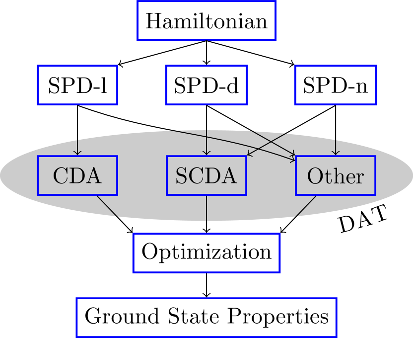
Figure 9: A schematic of the VDAT workflow.

VII.2 Parameterization of the SPD

An SPD will normally contain a large number of variational parameters, potentially even infinite. Our definition of an SPD dictates that the non-interacting SPD has full variational freedom, and then in practice one can decide whether or not to exploit all of it. We emphasize that this philosophy sometimes departs with common practices in related variational wave functions, such as in the case of the Baeriswyl wave function (i.e. $\mathcal{N}=2$, B-type SPD), which typically only has a single variational parameter for the kinetic projectors[41, 55]. Alternatively, for Hartree-Fock (i.e. $\mathcal{N}=1$, G-type SPD), full variational freedom for the non-interacting projectors is exploited. In any case, we have proven that for $\mathcal{N}\geq 3$, even very naive schemes for parameterizing the space of non-interacting variational parameters in terms of a small number of variables can give highly precise results[20]. We will present examples in the context of the Hubbard model and AIM to illustrate these ideas.

In terms of the interacting projector, the number of variational parameters could be as large as the Fock space that the interacting projectors span, which can be impractical even in principle; or it could be as small as one variational parameter, which would still recover the exact solution in the large $\mathcal{N}$ limit. In the examples considered below, we will only be evaluating a single interacting orbital, such that there is only a single variational parameter at each integer time. The remainder of this section focuses purely on parameterizing the non-interacting projector for applications with $\mathcal{N}\geq 3$, which have been used in our accompanying applications[20].

VII.2.1 Parameterization of SPD-l for the AIM on a ring

Here we consider the Anderson Impurity model (AIM) on a ring[46], given by

$$\hat{H}=\hat{H}_{0}+\hat{V},\hskip 10.00002pt\hat{V}=U\left(\hat{f}_{\uparrow}^{\dagger}\hat{f}_{\uparrow}-\frac{1}{2}\right)\left(\hat{f}_{\downarrow}^{\dagger}\hat{f}_{\downarrow}-\frac{1}{2}\right),$$ (326)

$$\hat{H}_{0}=v\sum_{\sigma}(\hat{f}_{\sigma}^{\dagger}\hat{c}_{0,\sigma}+h.c.)-\frac{W}{4}\sum_{\sigma,n=0}^{L-1}\left(\hat{c}_{n,\sigma}^{\dagger}\hat{c}_{n+1,\sigma}+h.c\right).$$ (327)

The interacting projector of the SPD-l is given as

$$\hat{P}_{\tau} =P_{\tau,0}\hat{X}_{0}+P_{\tau,\downarrow}\hat{X}_{\downarrow}+P_{\tau,\uparrow}\hat{X}_{\uparrow}+P_{\tau,\uparrow\downarrow}\hat{X}_{\uparrow\downarrow}$$ (328)

$$=(1-\mu_{\tau}-\frac{1}{4}u_{\tau})\hat{1}+\mu_{\tau}\sum_{\sigma}\hat{f}_{\sigma}^{\dagger}\hat{f}_{\sigma}+u_{\tau}\hat{f}_{\uparrow}^{\dagger}\hat{f}_{\uparrow}\hat{f}_{\downarrow}^{\dagger}\hat{f}_{\downarrow},$$ (329)

where $\hat{X}_{\Gamma}$ are diagonal Hubbard operators and $P_{\tau,\Gamma}$ are variational parameters, which can then be constrained using the density and normalization. For this case of spin symmetry, we formally have two variational parameters $u_{\tau}$ and $\mu_{\tau}$ for each time step, though the latter should be considered as a parameter to constrain the local density.

For the non-interacting projector, we allow for three variational parameters: one for each independent parameter in the non-interacting Hamiltonian, though one parameter will be fixed by the total density. In order to implement this, it is most convenient to use a diagonal form, so we construct an effective basis which is a function of the three variational parameters, which then allows us to enforce a semi-definite matrix. The non-interacting projector is given by

$$\exp\left(\bm{\gamma}_{\tau}\cdot\hat{\bm{n}}\right)=\prod_{j\sigma}\big{(}(1+h(\epsilon_{j\sigma;\tau})(\hat{b}_{j\sigma}^{\dagger}\hat{b}_{j\sigma}-\frac{1}{2})\big{)},$$ (330)

where $\epsilon_{j\sigma;\tau}$ are functions of the variational parameters given by

$$\sum_{j\sigma}\epsilon_{j\sigma;\tau}\hat{b}_{j\sigma}^{\dagger}\hat{b}_{j\sigma}=\eta_{1;\tau}\sum_{\sigma}\left(\hat{f}_{\sigma}^{\dagger}\hat{c}_{0,\sigma}+h.c.\right)-$$

$$\eta_{2;\tau}\sum_{\sigma,n=0}^{L-1}\left(\hat{c}_{n,\sigma}^{\dagger}\hat{c}_{n+1,\sigma}+h.c\right)+\eta_{3;\tau}\hat{N},$$ (331)

and $\eta_{1;\tau},\eta_{2;\tau},\eta_{3;\tau}$ are the variational parameters, the indices $j,\sigma$ label the eigenstates of the above diagonalized form, and the function $h$ is defined as

$$h(x)=\begin{cases}2,&x>2\\ x,&-2<x\leq 2\\ -2,&x\leq-2.\end{cases}$$ (332)

VII.2.2 Parameterization of the SPD-d for the Hubbard model

Here we consider the single-band Hubbard model in an arbitrary dimension, defined as

$$\hat{H}=\sum_{ij\sigma}t_{ij}\hat{a}_{i\sigma}^{\dagger}\hat{a}_{j\sigma}+U\sum_{i}\hat{d}_{i},$$ (333)

where $\hat{d}_{i}=\hat{n}_{i\uparrow}\hat{n}_{i\downarrow}$, and we employ the SPD-d with local interacting projectors

$$\hat{P}_{\tau} =\prod_{i}\big{(}(1-\mu_{\tau}-\frac{1}{4}u_{\tau})\hat{1}+\mu_{\tau}\sum_{\sigma}\hat{n}_{i\sigma}+u_{\tau}\hat{d}_{i}\big{)},$$ (334)

where $\hat{P}_{\tau}$ is a product of local projectors with the same form as Eq. 329, and translation symmetry has been assumed.

The non-interacting projector for this SPD-d is simpler than the case of the SPD-l for the AIM, presented in the preceding section, given that translation symmetry fully diagonalizes the non-interacting Hamiltonian. In this case, we choose four variational parameters, allowing more freedom than the non-interacting form of the Hamiltonian, which only has nearest neighbor hopping. We have the following form for the non-interacting projector

$$\exp\left(\bm{\gamma}_{\tau}\cdot\hat{\bm{n}}\right)=\prod_{\mathbf{k}\sigma}\left(1+h(w_{\mathbf{k}\sigma;\tau})(\hat{n}_{\mathbf{k}\sigma}-\frac{1}{2})\right),$$ (335)

where

$$w_{\mathbf{k}\sigma;\tau}=\eta_{1}\theta(\epsilon_{\mathbf{k}\sigma}-\eta_{2})+\eta_{3}f(\epsilon_{\mathbf{k}\sigma}-\eta_{2},\eta_{4})+\eta_{2},$$ (336)

$$f(x,\alpha)=\textrm{sign}(x)(1-\exp(-\alpha|x|))/(1-\exp(-\alpha)).$$ (337)

where $h(x)$ is defined in Eq. 332 and the four variational parameters are $\eta_{i}$. The form of $w_{\mathbf{k}\sigma;\tau}$ is chosen such that it recovers the Baeriswyl kinetic projector when $\eta_{1}=0$ and $\eta_{4}\rightarrow 0$, thus allowing extra variational freedom. This particular form was motivated by examining the density distribution within perturbation theory. However, even when restricting to $\eta_{2}$ and $\eta_{3}$, the results for the ground state energy are nearly unchanged.

VIII Summary and Conclusions

In this work, we have introduced the variational discrete action theory (VDAT), which is a systematic variational approach for solving the ground state of quantum many-body Hamiltonians. VDAT consists of two important components: a variational ansatz referred to as the sequential product density matrix (SPD) and a general formalism to compute observables under the SPD, where the latter is referred to as the discrete action theory (DAT). It should be emphasized that when DAT exactly evaluates the energy of some Hamiltonian under the SPD, the result is a rigorous upper bound to the exact ground state energy, and minimization over the variational parameters within the SPD will provide the optimal solution for the SPD at a given $\mathcal{N}$. While for typical discretized Green’s function approaches, such as auxiliary field quantum Monte-Carlo, a large number of time steps are required, VDAT can provide remarkably accurate ground state results even for very small $\mathcal{N}$.

The SPD is clearly inspired by the Trotter-Suzuki decomposition, and the essence of the idea in the context of variational wave functions can be traced back to the work of Baeriswyl and coworkers decades ago[19]. However, without a clear prescription for evaluation, it is a tool of limited applicability; and the discrete action theory put forward in this paper greatly extends the reach of the SPD. In this paper, we put forward the most generic notion of an SPD, which can be partitioned into unitary, projective, and general cases. There are always two ways to constrain the SPD to be Hermitian and semi-definite: Gutzwiller-type and Baeriswyl-type, denoted G-type and B-type. We introduced three important classes of SPD in this work: the local SPD (SPD-l), the disjoint SPD (SPD-d), and the n-particle SPD (SPD-n). The key characteristic of an SPD-l is that it has a finite number of local interacting projectors, and the SPD-l is naturally applied to models where the interactions are restricted to some subspace, like the Anderson impurity model. Alternatively, the SPD-d has multiple sets of local interacting projectors which do not overlap, and the SPD-d is naturally applied to interacting lattice model like the Hubbard model or periodic Anderson model. The SPD-n has a general n-particle interacting projector, and the n=2 case would naturally apply to models with long range Coulomb repulsion.

In order to evaluate observables under the SPD, we introduced the integer time Green’s function formalism, which can be generally characterized by a discrete action. We demonstrate that for the SPD-l, one can sum all local diagrams, allowing for the exact evaluation of observables under the SPD-l, and illustrations for $\mathcal{N}\leq 2$ are provided for the AIM. To evaluate the SPD-d, the more advanced tools of many-body physics had to be generalized to our integer time formalism. We first generalized the path integral to integer time, demonstrating that integer time correlation functions under the SPD are equivalent to a static correlation function in a compound Fock space under an effective density matrix. Just as in the case of the usual path integral, the integer time case unifies the role of spatial and temporal degrees of freedom, allowing a straightforward generalization of the generating functional, Dyson equation, and Bethe-Salpeter equation to integer time.

We introduced a hierarchical scheme to categorize three types of discrete actions: the sequential discrete action (SDA), the canonical discrete action (CDA), and the general discrete action (GDA); where we the former is always a subset of the latter. The SDA is the discrete action of an SPD, which is a product of three operators in the compound space: a shift matrix $̱\hat{Q}$, a promoted sequential product of non-interacting projectors, and a promoted sequential product of interacting projectors. For the SDA, only $̱\hat{Q}$ introduces correlations between different integer times, while the other two components are integer time blocked. The CDA, is a product of two operators in the compound space: a general non-interacting projector and a promoted sequential product of interacting projectors. For the CDA, only the non-interacing projector introduces correlations between different integer times, while the interacting projectors are integer time blocked. The GDA is a general operator in the compound space.

A key step forward in this paper is the self-consistent canonical discrete action approximation (SCDA), which is the integer time generalization of the dynamical mean-field theory. In general, the SPD-d cannot be exactly evaluated. However, we prove that in $d=\infty$, the SPD-d can be exactly mapped to a CDA with a self-consistently determined non-interacting integer time Green’s function. Therefore, the SPD-d can be exactly evaluated for the Hubbard model in $d=\infty$, making VDAT a potent tool for solving the multi-band Hubbard model. For $\mathcal{N}=2$, this recovers the classic result that the Gutzwiller approximation exactly evaluates the Gutzwiller wave function in $d=\infty$[14, 15, 16, 17]. For $\mathcal{N}=3$, this proves that both the Gutzwiller-Baeriswyl and the Baeriswyl-Gutzwiller wave functions can be exactly evaluate in $d=\infty$. For $\mathcal{N}\geq 4$, this yields new variational wave functions that can be exactly evaluated in $d=\infty$ (see Reference 20 for applications). The VDAT gives a long awaited variational understanding of $d=\infty$, which traditionally necessitated the use of Green’s function based approaches. The SPD-d within the SCDA can also be applied as an approximation in finite dimensions, improving upon well characterized theories such as the Gutzwiller approximation.

The VDAT formalism unifies many seemingly disparate variational wave functions, connecting Hartree-Fock, the Gutzwiller wave function, etc, all into the same framework, while putting forward an infinite number of extensions. Equally importantly, the integer time Green’s function and the discrete action theory provides a paradigm for generalizing concepts from the standard many-body Green’s functions methods. For example, once the general formalism was identified, it was obvious how to realize the dynamical mean-field theory in the integer time formalism, allowing for remarkably accurate results at $\mathcal{N}=3$[20].

There are many near term and far term directions to consider for VDAT. In the near term, the multi-band Hubbard model is the most obvious target. Given that the Gutzwiller approximation is known to produce reasonable results in the Fermi-liquid regime of the multi-band Hubbard model[56, 49], and that we know VDAT($\mathcal{N}=3$) precisely captures the metallic and insulating regime of the one band model in $d=\infty$[20], VDAT($\mathcal{N}=3$) within the SCDA should be sufficiently accurate for the multi-band case. Further applications could include novel approaches for evaluating the SPD-d in low dimensions using quantum Monte-Carlo, which would expand upon the recent work of Baeriswyl in the 2d Hubbard model[45], which in our language was a perturbative evaluation of a G-type SPD-d at $\mathcal{N}=3$. Other interesting applications include the homogeneous electron gas, which could require the use of an integer time generalized auxiliary field QMC to evaluate the SPD-2. In terms of further methodological developments, it will be useful to consider finite temperatures, where one must develop approaches for evaluating the entropy. Furthermore, it will be useful to extend the Landau-Gutzwiller quasiparticle approach[28] in the context of VDAT, such that excited state properties can be treated.

IX Acknowledgments

This work was supported by the grant DE-SC0016507 funded by the U.S. Department of Energy, Office of Science. This research used resources of the National Energy Research Scientific Computing Center, a DOE Office of Science User Facility supported by the Office of Science of the U.S. Department of Energy under Contract No. DE-AC02-05CH11231.

X Appendix

X.1 Lie group properties of non-interacting systems

In this appendix, we study the properties of the density matrices that are exponentially generated from single particle potentials, and this applies equally both to the physical Fock space and the compound space (see Section IV.2). Understanding these objects is critical given that they are the noninteracting projectors of the SPD. We start with a system containing $L$ spin orbitals, and we define a generalized non-interacting many-body density matrix as

$$\hat{\rho}\left(\boldsymbol{v}\right)=\exp(\boldsymbol{v}\cdot\hat{\bm{n}})=\exp\bigg{(}\sum_{ij}v_{ij}\hat{a}_{i}^{\dagger}\hat{a}_{j}\bigg{)},$$ (338)

and we refer to this as generalized because $v_{ij}$ forms a complex matrix that is not necessarily Hermitian. In order to understand that this operator can be viewed as being generated from a Lie algebra, we rewrite Eq. 338 in the form

$$\hat{\rho}\left(\boldsymbol{v}\right)=\exp(\sum_{\Gamma}v_{\Gamma}\hat{O}_{\Gamma}),$$ (339)

where $\Gamma=\left(i,j\right)$ and $\hat{O}_{\left(i,j\right)}=\hat{a}_{i}^{\dagger}\hat{a}_{j}$. From the anti-commutation relation $\{\hat{a}_{i}^{\dagger},\hat{a}_{j}\}=\delta_{ij}$, we deduce

$$\left[\hat{O}_{\left(i,j\right)},\hat{O}_{\left(k,l\right)}\right] =\hat{O}_{\left(i,l\right)}\delta_{kj}-\hat{O}_{\left(k,j\right)}\delta_{il}.$$ (340)

Therefore, the operators $\hat{O}_{\Gamma}$ form a Lie algebra and $\hat{\rho}\left(\boldsymbol{v}\right)$ form a Lie group. This Lie group structure has long been recognized[57, 58], though previous application did not consider non-Hermitian cases.

It is impractical to directly compute the non-interacting density matrix in the Fock space for a large system, and therefore we need a more efficient approach, which can be achieved by finding an isomorphism of the Lie algebra $\hat{O}_{\Gamma}\leftrightarrow A_{\Gamma}$. The matrices $A_{\Gamma}$ are defined as

$$[A_{(i,j)}]_{ml}=\delta_{im}\delta_{jl},$$ (341)

and have dimension $L\times L$. The commutation relations are given as

$$\left[A_{\left(i,j\right)},A_{\left(k,l\right)}\right] =A_{\left(i,l\right)}\delta_{k,j}-A_{\left(k,j\right)}\delta_{il},$$ (342)

which have the same commutation relations as $\hat{O}_{\left(i,j\right)}$, proving the isomorphism. Therefore, we have the map

$$\hat{\rho}\left(\boldsymbol{v}\right) = \exp\left(\sum_{\Gamma}v_{\Gamma}\hat{O}_{\Gamma}\right)$$ (343)

$$\updownarrow$$

$$\exp\left(\boldsymbol{v}\right) = \exp\left(\sum_{\Gamma}v_{\Gamma}A_{\Gamma}\right).$$ (344)

The single-particle density matrix is defined as

$$\boldsymbol{n}\left(\boldsymbol{v}\right) =\langle\hat{\bm{n}}\rangle_{\hat{\rho}(\boldsymbol{v})}=\begin{pmatrix}\langle\hat{a}_{1}^{\dagger}\hat{a}_{1}\rangle_{\hat{\rho}(\boldsymbol{v})}&\dots&\langle\hat{a}_{1}^{\dagger}\hat{a}_{L}\rangle_{\hat{\rho}(\boldsymbol{v})}\\ \dots&\dots&\dots\\ \langle\hat{a}_{L}^{\dagger}\hat{a}_{1}\rangle_{\hat{\rho}(\boldsymbol{v})}&\dots&\langle\hat{a}_{L}^{\dagger}\hat{a}_{L}\rangle_{\hat{\rho}(\boldsymbol{v})}\end{pmatrix}$$ (345)

$$=\left(\frac{\boldsymbol{1}}{\boldsymbol{1}+\exp\left(-\boldsymbol{v}\right)}\right)^{T}.$$ (346)

The above equation can be derived as following, starting with

$$\text{Tr}\left(\hat{\rho}\left(\boldsymbol{v}\right)\right)=\text{det}\left(\boldsymbol{1}+\exp\left(\boldsymbol{v}\right)\right),$$ (347)

and writing the single particle density matrix as a derivative, we have

$$\boldsymbol{n}\left(\bm{v}\right) =\frac{\partial\ln\left(\text{Tr}\left(\hat{\rho}\left(\bm{v}\right)\right)\right)}{\partial\bm{v}}=\frac{\partial\ln\left(\text{det}\left(\boldsymbol{1}+\exp\left(\bm{v}\right)\right)\right)}{\partial\bm{v}}$$ (348)

$$=\frac{\partial\text{Tr}\left(\text{$\ln$}\left(\boldsymbol{1}+\exp\left(\bm{v}\right)\right)\right)}{\partial\bm{v}}=\left(\frac{\boldsymbol{1}}{\boldsymbol{1}+\exp\left(-\bm{v}\right)}\right)^{T}.$$ (349)

Now we consider group multiplication in terms of $\bm{n}$. We begin by parametrizing the group element in terms of $\bm{n}$ as

$$\exp\left(\bm{v}\right)=\left(\frac{\boldsymbol{1}}{\bm{n}\left(\bm{v}\right)^{-1}-\boldsymbol{1}}\right)^{T},$$ (350)

and recalling the group multiplication

$$\exp\left(\bm{v}\right)=\exp\left(\bm{v}_{1}\right)\exp\left(\bm{v}_{2}\right),$$ (351)

we then have

$$\left(\bm{n}^{-1}-\bm{1}\right)=\left(\bm{n}_{1}^{-1}-\bm{1}\right)\left(\bm{n}_{2}^{-1}-\bm{1}\right),$$ (352)

and solving for $\boldsymbol{n}$ we have

$$\bm{n}=\bm{n}_{2}\left(\bm{1}-\bm{n}_{1}-\bm{n}_{2}+2\bm{n}_{1}\bm{n}_{2}\right)^{-1}\bm{n}_{1}=\bm{n}_{1}\star\bm{n}_{2}.$$ (353)

Finally, we have the group multiplication rules in terms of $\bm{n}$. This is very useful given that we will normally parameterize the non-interacting projector in terms of the single particle density matrix instead of the potential $\boldsymbol{v}$.

Recall that the integer time Green’s function is a non-Hermitian single-particle density matrix in the compound space. Therefore, the preceding derivations will greatly facilitate the manipulation of the integer time Green’s function. Consider a non-interacting SPD $\hat{\varrho}=\mathcal{\hat{P}}_{1}...\mathcal{\hat{P}}_{\mathcal{N}}$, with $\mathcal{\hat{P}}_{\tau}=\exp\left(\bm{\gamma}_{\tau}\cdot\hat{\bm{n}}\right)$, which can be reparameterized using

$$\boldsymbol{n}_{\tau}=\left(\frac{\boldsymbol{1}}{\boldsymbol{1}+\exp\left(-\bm{\gamma}_{\tau}\right)}\right)^{T}.$$ (354)

Using the group notation, we can write the non-interacting integer time Green’s function as

$$\bm{g}_{0}=\bm{g}_{Q}\star\textrm{diag($\bm{n}_{1}$,..,$\bm{n}_{\mathcal{N}}$)},$$ (355)

where $\bm{g}_{Q}$ is defined in Eq. 117. For the special case of $\mathcal{N}=2$, we have

$$\bm{g}_{0}=\begin{pmatrix}\bm{n}_{2}\star\bm{n}_{1}&\left(\bm{n}_{2}^{-1}-\bm{1}\right)\bm{n}_{1}\star\bm{n}_{2}\\ -\left(\bm{n}_{1}^{-1}-\bm{1}\right)\bm{n}_{2}\star\bm{n}_{1}&\bm{n}_{1}\star\bm{n}_{2}\end{pmatrix}.$$ (356)

The preceding case is very important for a non-interacting SPD at a general $\mathcal{N}$ given that one can always split the sequential integer time blocks into two parts, and iteratively apply Eq. 356 using

$$\hat{\varrho}^{\prime}=\left(\mathcal{\hat{P}}_{j+1}...\mathcal{\hat{P}}_{i-1}\mathcal{\hat{P}}_{i}\right)\left(\mathcal{\hat{P}}_{i+1}..\mathcal{\hat{P}}_{j}\right)=\mathcal{\hat{P}}^{\prime}_{1}\mathcal{\hat{P}}^{\prime}_{2}.$$ (357)

X.2 Proof of the integer time Wick’s theorem

Wick’s theorem is an important tool for evaluating expectation values in a non-interacting system, and it is imperative to generalize this to the integer time formalism. We begin by introducing a unified notation for creation and annihilation operators as

$$\hat{A}_{i\theta}=\begin{cases}\hat{a}_{i}^{\dagger},&\theta=0\\ \hat{a}_{i},&\theta=1\end{cases}.$$ (358)

Next, we consider how to commute $\hat{A}_{i\theta}$ with the non-interacting density matrix (see Subsection II.2)

$$\hat{A}_{i\theta}\exp\left(\bm{v}\cdot\hat{\bm{n}}\right)=M_{i\theta,i^{\prime}\theta^{\prime}}\left(\bm{v}\right)\exp\left(\bm{v}\cdot\hat{\bm{n}}\right)\hat{A}_{i^{\prime}\theta^{\prime}},$$ (359)

where

$$M_{i\theta,i^{\prime}\theta^{\prime}}\left(\bm{v}\right)=\begin{cases}\left[\exp\left(-\bm{v}^{T}\right)\right]_{ii^{\prime}}\delta_{\theta,\theta^{\prime}},&\theta=0\\ \left[\exp\left(\bm{v}\right)\right]_{ii^{\prime}}\delta_{\theta,\theta^{\prime}},&\theta=1\end{cases}$$ (360)

and Einstein notation is employed throughout this section. Note that the above can be further generalized by considering pairing terms, which have not presently been included in $\hat{\bm{n}}$. Recall the integer time Heisenberg representation for the non-interacting SPD

$$\hat{A}_{i\theta}\left(\tau\right)=U_{\tau}\hat{A}_{i\theta}U_{\tau}^{-1},$$ (361)

where

$$U_{\tau}=\exp\left(\bm{v}_{1}\cdot\hat{\bm{n}}\right)...\exp\left(\bm{v}_{\tau}\cdot\hat{\bm{n}}\right)=\exp\left(V_{1,\tau}\cdot\hat{\bm{n}}\right).$$ (362)

We can then use Eq. 359 and Eq. 361 to find

$$\hat{A}_{i\theta}=M_{i\theta,i^{\prime}\theta^{\prime}}(V_{1,\tau})\hat{A}_{i^{\prime}\theta^{\prime}}(\tau),$$ (363)

$$\hat{A}_{i\theta}(\tau)=M_{i\theta,i^{\prime}\theta^{\prime}}(-V_{1,\tau})\hat{A}_{i^{\prime}\theta^{\prime}}.$$ (364)

For $\tau_{1}\leq\tau_{2}$, we then have

$$\hat{A}_{i\theta}(\tau_{2}) =M_{i\theta,i^{\prime}\theta^{\prime}}(-V_{1,\tau_{2}})\hat{A}_{i^{\prime}\theta^{\prime}}$$ (365)

$$=M_{i\theta,i^{\prime}\theta^{\prime}}(-V_{1,\tau_{2}})M_{i^{\prime}\theta^{\prime},i^{\prime\prime}\theta^{\prime\prime}}(V_{1,\tau_{1}})\hat{A}_{i^{\prime\prime}\theta^{\prime\prime}}(\tau_{1}).$$ (366)

Recalling the Lie group isomorphism

$$M\left(V\right)\leftrightarrow\exp\left(V\right)$$ (367)

and the identity

$$\exp\left(-V_{1,\tau_{2}}\right)\exp\left(V_{1,\tau_{1}}\right)=\exp\left(-V_{\tau_{1}+1,\tau_{2}}\right),$$ (368)

where

$$\exp\left(\bm{v}_{\tau_{1}}\right)...\exp\left(\bm{v}_{\tau_{2}}\right)=\exp\left(V_{\tau_{1},\tau_{2}}\right),$$ (369)

we then have

$$M_{i\theta,i^{\prime}\theta^{\prime}}(-V_{1,\tau_{2}})M_{i^{\prime}\theta^{\prime},i^{\prime\prime}\theta^{\prime\prime}}\left(V_{1,\tau_{1}}\right)$$

$$=M_{i\theta,i^{\prime\prime}\theta^{\prime\prime},}(-V_{\tau_{1}+1,\tau_{2}}),$$ (370)

which yields

$$\hat{A}_{i\theta}(\tau_{2})=M_{i\theta,i^{\prime}\theta^{\prime}}(-V_{\tau_{1}+1,\tau_{2}})\hat{A}_{i^{\prime}\theta^{\prime}}(\tau_{1}),$$ (371)

$$\hat{A}_{i\theta}\left(\tau_{1}\right)=M_{i\theta,i^{\prime}\theta^{\prime}}(V_{\tau_{1}+1,\tau_{2}})\hat{A}_{i^{\prime}\theta^{\prime}}(\tau_{2}).$$ (372)

We also have

$$\left\{\hat{A}_{i\theta}\left(\tau\right),\hat{A}_{i^{\prime}\theta^{\prime}}\left(\tau\right)\right\}=\delta_{ii^{\prime}}\delta_{\theta+\theta^{\prime},1}\equiv\Delta_{i\theta,i^{\prime}\theta^{\prime}}.$$ (373)

Considering $\tau_{1}\leq\tau_{2}$ and $\bm{v}_{i+\mathcal{N}}=\bm{v}_{i}$, we have

$$\langle\hat{A}_{i_{1}\theta_{1}}(\tau_{1})\hat{A}_{i_{2}\theta_{2}}(\tau_{2})\rangle$$

$$=M_{i_{1}\theta_{1},i^{\prime}_{1}\theta^{\prime}_{1}}(V_{\tau_{1}+1,\tau_{2}})\langle\hat{A}_{i^{\prime}_{1}\theta^{\prime}_{1}}(\tau_{2})\hat{A}_{i_{2}\theta_{2}}(\tau_{2})\rangle$$ (374)

$$=M_{i_{1}\theta_{1},i^{\prime}_{1}\theta^{\prime}_{1}}(V_{\tau_{1}+1,\tau_{2}})\Delta_{i^{\prime}_{1}\theta^{\prime}_{1},i^{\prime}_{2}\theta^{\prime}_{2}}-$$

$$M_{i_{1}\theta_{1},i^{\prime}_{1}\theta^{\prime}_{1}}(V_{\tau_{1}+1,\tau_{2}})\langle\hat{A}_{i_{2}\theta_{2}}(\tau_{2})\hat{A}_{i^{\prime}_{1}\theta^{\prime}_{1}}(\tau_{2})\rangle$$ (375)

$$=M_{i_{1}\theta_{1},i^{\prime}_{1}\theta^{\prime}_{1}}(V_{\tau_{1}+1,\tau_{2}})\Delta_{i^{\prime}_{1}\theta^{\prime}_{1},i_{2}\theta_{2}}-$$

$$M_{i_{1}\theta_{1},i^{\prime}_{1}\theta^{\prime}_{1}}(V_{\tau_{1}+1,\tau_{1}+\mathcal{N}})\langle\hat{A}_{i_{2}\theta_{2}}(\tau_{2})\hat{A}_{i^{\prime}_{1}\theta^{\prime}_{1}}(\tau_{1}+\mathcal{N})\rangle$$ (376)

$$=M_{i_{1}\theta_{1},i^{\prime}_{1}\theta^{\prime}_{1}}(V_{\tau_{1}+1,\tau_{2}})\Delta_{i^{\prime}_{1}\theta^{\prime}_{1},i_{2}\theta_{2}}-$$

$$M_{i_{1}\theta_{1},i^{\prime}_{1}\theta^{\prime}_{1}}(V_{\tau_{1}+1,\tau_{1}+\mathcal{N}})\langle\hat{A}_{i^{\prime}_{1}\theta^{\prime}_{1}}(\tau_{1})\hat{A}_{i_{2}\theta_{2}}(\tau_{2})\rangle.$$ (377)

Therefore, we have

$$(\delta_{i_{1}\theta_{1},i^{\prime}_{1}\theta^{\prime}_{1}}+M_{i_{1}\theta_{1},i^{\prime}_{1}\theta^{\prime}_{1}}(V_{\tau_{1}+1,\tau_{1}+\mathcal{N}}))\langle\hat{A}_{i^{\prime}_{1}\theta^{\prime}_{1}}(\tau_{1})\hat{A}_{i_{2}\theta_{2}}(\tau_{2})\rangle$$

$$=M_{i_{1}\theta_{1},i^{\prime}_{1}\theta^{\prime}_{1}}(V_{\tau_{1}+1,\tau_{2}})\Delta_{i^{\prime}_{1}\theta^{\prime}_{1},i_{2}\theta_{2}},$$ (378)

and we can solve for the integer time Green’s function as

$$\langle\hat{A}_{i_{1}\theta{}_{1}}(\tau_{1})\hat{A}_{i_{2}\theta_{2}}(\tau_{2})\rangle=$$

$$\left[\frac{1}{1+M(V_{\tau_{1}+1,\tau_{1}+N})}M(V_{\tau_{1}+1,\tau_{2}})\Delta\right]_{i_{1}\theta_{1},i_{2}\theta_{2}}.$$ (379)

Now we consider how to evaluate the general case of an M-particle integer time Green’s function.

Considering the case where the $\tau_{i}$ are ordered and $N=2M$, we have

$$\langle\hat{A}_{i_{1}\theta_{1}}(\tau_{1})\hat{A}_{i_{2}\theta_{2}}(\tau_{2})...\hat{A}_{i_{N}\theta_{N}}(\tau_{N})\rangle$$

$$=M_{i_{1}\theta_{1},i^{\prime}_{1}\theta^{\prime}_{1}}(V_{\tau_{1}+1,\tau_{2}})\langle\hat{A}_{i^{\prime}_{1}\theta^{\prime}_{1}}(\tau_{2})\hat{A}_{i_{2}\theta_{2}}(\tau_{2})...\hat{A}_{i_{N}\theta_{N}}(\tau_{N})\rangle$$

$$=M_{i_{1}\theta_{1},i^{\prime}_{1}\theta^{\prime}_{1}}(V_{\tau_{1}+1,\tau_{2}})\times$$

$$\langle\big{(}\Delta_{i^{\prime}_{1}\theta^{\prime}_{1},i_{2}\theta_{2}}-\hat{A}_{i_{2}\theta_{2}}(\tau_{2})\hat{A}_{i^{\prime}_{1}\theta^{\prime}_{1}}(\tau_{2})\big{)}...\hat{A}_{i_{N}\theta_{N}}(\tau_{N})\rangle$$

$$=M_{i_{1}\theta_{1},i^{\prime}_{1}\theta^{\prime}_{1}}(V_{\tau_{1}+1,\tau_{2}})\Delta_{i^{\prime}_{1}\theta^{\prime}_{1},i_{2}\theta_{2}}\langle\hat{A}_{i_{3}\theta_{3}}(\tau_{3})...\hat{A}_{i_{N}\theta_{N}}(\tau_{N})\rangle$$

$$-M_{i_{1}\theta_{1},i^{\prime}_{1}\theta^{\prime}_{1}}(V_{\tau_{1}+1,\tau_{2}})\times$$

$$\langle\hat{A}_{i_{2}\theta_{2}}(\tau_{2})\hat{A}_{i^{\prime}_{1}\theta^{\prime}_{1}}(\tau_{2})\hat{A}_{i_{3}\theta_{3}}(\tau_{3})...\hat{A}_{i_{N}\theta_{N}}(\tau_{N})\rangle$$

$$=M_{i_{1}\theta_{1},i^{\prime}_{1}\theta^{\prime}_{1}}(V_{\tau_{1}+1,\tau_{2}})\Delta_{i^{\prime}_{1}\theta^{\prime}_{1},i_{2}\theta_{2}}\langle\hat{A}_{i_{3}\theta_{3}}(\tau_{3})...\hat{A}_{i_{N}\theta_{N}}(\tau_{N})\rangle$$

$$-M_{i_{1}\theta_{1},i^{\prime}_{1}\theta^{\prime}_{1}}(V_{\tau_{1}+1,\tau_{3}})\times$$

$$\langle\hat{A}_{i_{2}\theta_{2}}(\tau_{2})(\Delta_{i^{\prime}_{1}\theta^{\prime}_{1},i_{3}\theta_{3}}-\hat{A}_{i_{3}\theta_{3}}(\tau_{3})\hat{A}_{i^{\prime}_{1}\theta^{\prime}_{1}}(\tau_{3}))...\hat{A}_{i_{N}\theta_{N}}(\tau_{N})\rangle$$

$$=\sum_{\ell=2}^{N}\left(-1\right)^{\ell}M_{i_{1}\theta_{1},i^{\prime}_{1}\theta^{\prime}_{1}}(V_{\tau_{1}+1,\tau_{\ell}})\Delta_{i^{\prime}_{1}\theta^{\prime}_{1},i_{\ell}\theta_{\ell}}\times$$

$$\langle\hat{A}_{i_{2}\theta_{2}}(\tau_{2})...\hat{A}_{i_{\ell-1}\theta_{\ell-1}}(\tau_{\ell-1})\hat{A}_{i_{\ell+1}\theta_{\ell+1}}(\tau_{\ell+1})...\hat{A}_{i_{N}\theta_{N}}(\tau_{N})\rangle$$

$$-M_{i_{1}\theta_{1},i^{\prime}_{1}\theta^{\prime}_{1}}(V_{\tau_{1}+1,\tau_{1}+N})\times$$

$$\langle\hat{A}_{i^{\prime}_{1}\theta^{\prime}_{1}}(\tau_{1})\hat{A}_{i_{2}\theta_{2}}(\tau_{2})...\hat{A}_{i_{N}\theta_{N}}(\tau_{N})\rangle.$$ (380)

Therefore, the M-particle Green’s function can be written as a summation of the product of a single-particle and $(M-1)$-particle integer time Green’s functions.

$$\langle\hat{A}_{i_{1}\theta_{1}}(\tau_{1})\hat{A}_{i_{2}\theta_{2}}(\tau_{2})...\hat{A}_{i_{N}\theta_{N}}(\tau_{N})\rangle$$

$$=\sum_{\ell=2}^{N}\left(-1\right)^{\ell}\langle\hat{A}_{i_{1}\theta_{1}}(\tau_{1})\hat{A}_{i_{\ell}\theta_{\ell}}(\tau_{\ell})\rangle\times$$

$$\langle\hat{A}_{i_{2}\theta_{2}}(\tau_{2})..\hat{A}_{i_{\ell-1}\theta_{\ell-1}}(\tau_{\ell-1})\hat{A}_{i_{\ell+1}\theta_{\ell+1}}(\tau_{\ell+1})...\hat{A}_{i_{N}\theta_{N}}(\tau_{N})\rangle.$$ (381)

Iteratively applying the preceding equation proves Wick’s theorem.

References

• Jastrow [1955] R. Jastrow, Phys. Rev. 98, 1479 (1955).
• Capello et al. [2005] M. Capello, F. Becca, M. Fabrizio, S. Sorella,  and E. Tosatti, Phys. Rev. Lett. 94, 026406 (2005).
• Bartlett et al. [1989] R. J. Bartlett, S. A. Kucharski,  and J. Noga, Chemical Physics Letters 155, 133 (1989).
• Kutzelnigg [1991] W. Kutzelnigg, Theoretica Chimica Acta 80, 349 (1991).
• Taube and Bartlett [2006] A. G. Taube and R. J. Bartlett, International Journal Of Quantum Chemistry 106, 3393 (2006).
• Trotter [1959] H. F. Trotter, Proceedings of the American Mathematical Society 10, 545 (1959).
• Suzuki [1976] M. Suzuki, Communications In Mathematical Physics 51, 183 (1976).
• Suzuki [1993] M. Suzuki, Physica A-statistical Mechanics And Its Applications 194, 432 (1993).
• Hubbard [1959] J. Hubbard, Phys. Rev. Lett. 3, 77 (1959).
• Blankenbecler et al. [1981] R. Blankenbecler, D. J. Scalapino,  and R. L. Sugar, Physical Review D 24, 2278 (1981).
• Gutzwiller [1963] M. C. Gutzwiller, Phys. Rev. Lett. 10, 159 (1963).
• Gutzwiller [1964] M. C. Gutzwiller, Physical Review 134, 923 (1964).
• Gutzwiller [1965] M. C. Gutzwiller, Physical Review 137, 1726 (1965).
• Metzner and Vollhardt [1987] W. Metzner and D. Vollhardt, Phys. Rev. Lett. 59, 121 (1987).
• Metzner and Vollhardt [1988] W. Metzner and D. Vollhardt, Phys. Rev. B 37, 7382 (1988).
• Metzner and Vollhardt [1989] W. Metzner and D. Vollhardt, Phys. Rev. Lett. 62, 324 (1989).
• Bunemann et al. [1997] J. Bunemann, F. Gebhard,  and W. Weber, Journal Of Physics-condensed Matter 9, 7343 (1997).
• Otsuka [1992] H. Otsuka, J. Phys. Soc. Jpn. 61, 1645 (1992).
• Dzierzawa et al. [1995] M. Dzierzawa, D. Baeriswyl,  and M. Distasio, Phys. Rev. B 51, 1993 (1995).
• Cheng and Marianetti [2020a] Z. Cheng and C. A. Marianetti, Phys. Rev. Lett. [jointly submitted with current manuscript] 0, 0 (2020a).
• Georges et al. [1996] A. Georges, G. Kotliar, W. Krauth,  and M. J. Rozenberg, Rev. Mod. Phys. 68, 13 (1996).
• Kotliar and Vollhardt [2004] G. Kotliar and D. Vollhardt, Physics Today 57, 53 (2004).
• Vollhardt [2012] D. Vollhardt, Annalen Der Physik 524, 1 (2012).
• Kotliar et al. [2006] G. Kotliar, S. Y. Savrasov, K. Haule, V. S. Oudovenko, O. Parcollet,  and C. A. Marianetti, Rev. Mod. Phys. 78, 865 (2006).
• Wang et al. [2010] W. S. Wang, X. M. He, D. Wang, Q. H. Wang, Z. D. Wang,  and F. C. Zhang, Phys. Rev. B 82, 125105 (2010).
• Sandri et al. [2013] M. Sandri, M. Capone,  and M. Fabrizio, Phys. Rev. B 87, 205108 (2013).
• Lanata et al. [2015] N. Lanata, X. Y. Deng,  and G. Kotliar, Phys. Rev. B 92, 081108 (2015).
• Bunemann et al. [2003] J. Bunemann, F. Gebhard,  and R. Thul, Physical Review B 67, 075103 (2003).
• [29] See Supplemental Material at [URL will be inserted by publisher] for analytic results of the CDA for one orbital at $\mathcal{N}=3$.
• Hirsch [1983] J. E. Hirsch, Phys. Rev. B 28, 4059 (1983).
• Hirsch and Fye [1986] J. E. Hirsch and R. M. Fye, Phys. Rev. Lett. 56, 2521 (1986).
• [32] Baeriswyl et al. have also presented pedagogical results for the Hubbard plaquette using what is labeled as the Gutwziller wavefunction[45]. In this specific case, they choose an unprojected wavefunction which is a mixture of several Slater determinants; in contrast to usual applications.
• Cheng and Marianetti [2020b] Z. Cheng and C. A. Marianetti, Phys. Rev. B 101, 081105 (2020b).
• Fazekas and Penc [1988] P. Fazekas and K. Penc, International Journal of Modern Physics B 2, 1021 (1988).
• Yokoyama and Shiba [1990] H. Yokoyama and H. Shiba, J. Phys. Soc. Jpn. 59, 3669 (1990).
• Grimsley et al. [2019] H. R. Grimsley, S. E. Economou, E. Barnes,  and N. J. Mayhall, Nature Communications 10, 3007 (2019).
• Bartlett and Noga [1988] R. J. Bartlett and J. Noga, Chemical Physics Letters 150, 29 (1988).
• Ceperley et al. [1977] D. Ceperley, G. V. Chester,  and M. H. Kalos, Physical Review B 16, 3081 (1977).
• Sorella [2001] S. Sorella, Phys. Rev. B 64, 024512 (2001).
• Sorella [2005] S. Sorella, Phys. Rev. B 71, 241103 (2005).
• Baeriswyl [1987] D. Baeriswyl, in Nonlinearity in Condensed Matter, edited by A. R. Bishop, D. K. Campbell,  and S. E. Trullinger (Springer-Verlag, Berlin, 1987) 1st ed., pp. 183–193.
• Farhi et al. [2014] E. Farhi, J. Goldstone,  and S. Gutmann, arXiv:1411.4028  (2014).
• Wecker et al. [2015] D. Wecker, M. B. Hastings,  and M. Troyer, Physical Review A 92, 042303 (2015).
• Mahan [2000] G. D. Mahan, Many-Particle Physics (Physics of Solids and Liquids) (Springer, 2000).
• Baeriswyl [2019] D. Baeriswyl, Phys. Rev. B 99, 235152 (2019).
• Barcza et al. [2019] G. Barcza, F. Gebhard, T. Linneweber,  and O. Legeza, Phys. Rev. B 99, 165130 (2019).
• Harsha et al. [2018] G. Harsha, T. Shiozaki,  and G. E. Scuseria, Journal Of Chemical Physics 148, 044107 (2018).
• Negele and Orland [1998] J. W. Negele and H. Orland, Quantum Many-particle Systems (Perseus Books, 1998).
• Lanata et al. [2012] N. Lanata, H. Strand, X. Dai,  and B. Hellsing, Phys. Rev. B 85, 035133 (2012).
• Brinkman and Rice [1970] W. F. Brinkman and T. M. Rice, Physical Review B-solid State 2, 4302 (1970).
• Bunemann et al. [1998] J. Bunemann, W. Weber,  and F. Gebhard, Phys. Rev. B 57, 6896 (1998).
• Bunemann and Gebhard [2007] J. Bunemann and F. Gebhard, Phys. Rev. B 76, 193104 (2007).
• Bunemann et al. [2012] J. Bunemann, F. Gebhard, T. Schickling,  and W. Weber, Physica Status Solidi B-basic Solid State Physics 249, 1282 (2012).
• Aryasetiawan and Gunnarsson [1998] F. Aryasetiawan and O. Gunnarsson, Reports On Progress In Physics 61, 237 (1998).
• Baeriswyl et al. [2009] D. Baeriswyl, D. Eichenberger,  and M. Menteshashvili, New Journal Of Physics 11, 075010 (2009).
• Deng et al. [2009] X. Y. Deng, L. Wang, X. Dai,  and Z. Fang, Phys. Rev. B 79, 075114 (2009).
• Wybourne [1973] B. G. Wybourne, International Journal Of Quantum Chemistry 7, 1117 (1973).
• Fukutome et al. [1977] H. Fukutome, M. Yamamura,  and S. Nishiyama, Progress Of Theoretical Physics 57, 1554 (1977).