HexGen and Hex2Spline: Polycube-based Hexahedral Mesh Generation and Spline Modeling for Isogeometric Analysis Applications in LS-DYNA

Abstract

In this paper, we present two software packages, HexGen and Hex2Spline, that seamlessly integrate geometry design with isogeometric analysis (IGA) in LS-DYNA. Given a boundary representation of a solid model, HexGen creates a hexahedral mesh by utilizing a semi-automatic polycube-based mesh generation method. Hex2Spline takes the output hexahedral mesh from HexGen as the input control mesh and constructs volumetric truncated hierarchical splines. Through Bézier extraction, Hex2Spline transfers spline information to LS-DYNA and performs IGA therein. We explain the underlying algorithms in each software package and use a rod model to explain how to run the software. We also apply our software to several other complex models to test its robustness. Our goal is to provide a robust volumetric modeling tool and thus expand the boundary of IGA to volume-based industrial applications.

1 Introduction

Isogeometric analysis (IGA) Hughes is a computational technique that integrates computer aided design (CAD) with simulation methods such as finite element analysis (FEA). It adopts the idea of design-through-analysis and enables direct analysis of the designed geometry. IGA has many advantages over traditional FEA such as exact, smooth geometric representation and superior numerical performance. Many software packages have been developed for IGA and there are mainly two directions. The first direction is to incorporate IGA with commercial finite element software. For example, the user subroutine UEL in Abaqus is used to define IGA elements and perform IGA in Abaqus YicongLai2015 ; Lai2017 . The second direction is to develop open software packages. GeoPDEs deFalco20111020 and igatools pauletti2015igatools work on NURBS (Non-Uniform Rational B-Spline) patches and provide a general framework to implement IGA methods. PetIGA Dalcin2016 is another framework for IGA based on PETSc balay1997efficient . These software packages help boost the use of IGA in engineering applications. However, these packages are analysis-oriented. Currently, there is no available toolkit from the geometric modeling side, especially for volume parameterization. Therefore, the motivation of our work is to develop a geometric modeling tool to bridge the gap between geometric design and IGA analysis.

There are two major challenges in volume parameterization, control mesh generation and volumetric spline construction. A control mesh is generally an unstructured hexahedral (hex) mesh. Various strategies have been proposed in the literature ref:zhangbook for unstructured hex mesh generation, such as grid-based or octree-based schneiders1996grid ; S97 , medial surface Price1995 ; price1997hexahedral , plastering Blacker1991 ; SKOB06 , whisker weaving FM99 and vector field-based methods nieser2011cubecover . These methods have created hex meshes for certain geometries, but are not robust and reliable for arbitrary geometries. The polycube-based method Tarini2004 ; Gregson2011 is another appealing approach for all-hex meshing. A smooth harmonic field LeiLiu2012a was used to generate polycubes for arbitrary genus geometries. Boolean operations LZH2014 were introduced to cope with arbitrary genus geometries. In Liu2015 , polycube structure was generated based on the skeleton branches of a geometric model. For these methods, the hex mesh quality is directly affected by the polycube structure and mapping distortion. Computing the polycube structure with a low-distortion mapping remains an open problem for arbitrary geometries. It is essential to improve the mesh quality for analysis by using methods such as pillowing, smoothing and optimization qian2010quality ; YZhang2009c ; wenyan2011b ; qian2012automatic . Pillowing is a sheet insertion technique that eliminates the situations where two neighboring hex elements share more than one face. Smoothing and optimization are used to further improve mesh quality by relocating vertices. In our software, we implement all the above mentioned methods for quality improvement.

The second ingredient in volume parameterization is volumetric spline construction. Several algorithms have been developed. The initial development of IGA was based on NURBS. Since it adopts a global tensor-product structure, it does not support local refinement. T-splines were initially developed to support local refinement for surfaces ref:sederberg03 ; Sederberg1 . For solid models, the rational T-spline basis functions were used to convert unstructured hex meshes to solid T-splines Wenyan2011a . Boolean operations LZH2014 and skeletons Liu2015 are used to create hex meshes, which are later converted to T-meshes. However, local refinement using T-splines requires extensive mesh manipulation to satisfy desired properties such as linear independence. Hierarchical spline is an alternative to T-spline to avoid this issue. Several techniques were then developed based on hierarchical B-splines (HB-splines) ref:forsey88 ; ref:vuong11 , such as truncated hierarchical B-splines (THB-splines) ref_giannelli12 ; Giannelli2014 .

In this paper, we integrate our semi-automatic polycube-based mesh generation with the volumetric truncated hierarchical spline construction (TH-spline3D) wei17a to perform IGA on volumetric models in LS-DYNA. The developed software packages feature: 1) semi-automatic polycube-based all-hex mesh generation from a CAD model; 2) TH-spline3D construction on hex meshes; and 3) Bézier extraction for LS-DYNA. We first overview the entire pipeline and explain the algorithm behind each module of the pipeline. We then provide various examples to explain how to run the software package. The main objective of the software package is to make our pipeline accessible to industrial and academic communities who are interested in real-world engineering applications. Our software favors versatility over efficiency. We will use a concrete example to go through all the steps in running the software. In particular, when user intervention is needed, we will explain details of the involved manual work.

The paper is outlined as follows. In Section 2, we overview the pipeline. In Section 3, we present the HexGen software package that conducts semi-automatic polycube-based all-hex mesh generation from a CAD file. In Section 4, we talk about Hex2Spline that constructs TH-spline3D on hex meshes and performs Bézier extraction for IGA in LS-DYNA. Finally, in Section 5, we demonstrate several complex models using our software package.

2 Pipeline design

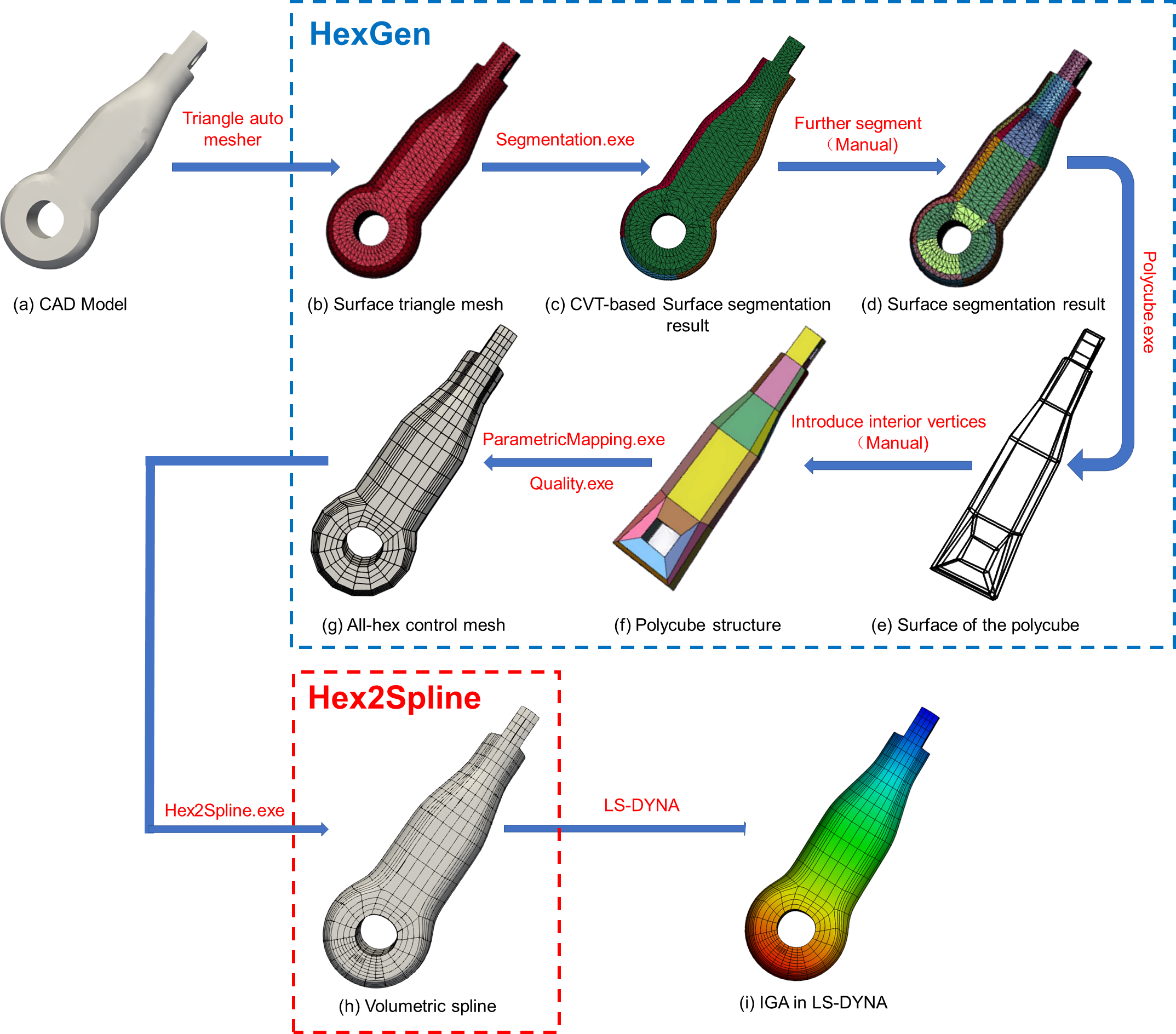
Figure 1: The HexGen software package and the Hex2Spline software package. The red text on each arrow shows the operation between two steps. The manual work is involved in further segmentation and introducing interior vertices.

Our pipeline incorporates two software packages to bridge the gap between the input CAD model with IGA in LS-DYNA, as shown in Fig. 1. We first use the HexGen software package to build an all-hex mesh for the CAD model. With a high quality all-hex mesh generated, we then use the Hex2Spline software package to construct TH-spline3D and extract Bézier information for LS-DYNA.

As shown in Fig. 1, we first generate a triangle mesh from the CAD model by using the free software LS-PrePost, which is a pre and post-processor for LS-DYNA. Then we use centroidal Voronoi tessellation (CVT) segmentation HZ2015CMAME to create a polycube structure Tarini2004 , which is used to generate all-hex meshes via parametric mapping floater1997 and octree subdivision wenyan2011b . The quality of the all-hex mesh is evaluated to ensure that the resulting volumetric spline model can be used in IGA. In case that a poor quality hex mesh is generated, the program has several quality improvement functions, including pillowing YZhang2009c , smoothing, and optimization qian2012automatic . Each quality improvement function can be run independently and one can use these functions to improve the mesh quality.

Once a good quality hex mesh is obtained, one can run the Hex2Spline program to build volumetric splines. In particular, TH-spline3D is built on the unstructured hex mesh and it also supports local refinement. The Hex2Spline can output the Bézier extraction information of TH-spline3D in a format that can be imported into LS-DYNA to perform IGA. Currently, our software only has a command-line interface (CLI). Users need to specify necessary options via the command line to run the software. In Sections 3 and 4, we will explain the algorithms implemented in each software as well as how to run the software in detail.

3 HexGen: Polycube-based hex mesh generation

Surface segmentation, polycube construction, parametric mapping, and octree subdivision are used together in the HexGen software package to construct an all-hex mesh from the boundary representation given by the input CAD model. Given an triangle mesh generated from the CAD model, we first use surface segmentation to divide the mesh into several surface patches that satisfy the polycube structure constraints, which will be discussed in Section 3.1. Then, the corner vertices, edges and face information of each surface patch are extracted from the surface segmentation result to construct a polycube structure. Each component of the polycube structure is topologically equivalent to a cube. Finally, we generate the all-hex mesh through parametric mapping and octree subdivision. Quality improvement techniques can be used to further improve the mesh quality.

In this section, we introduce the main algorithm for each module of the HexGen software package, namely surface segmentation, polycube construction, parametric mapping and octree subdivision, and quality improvement. We use a rod model (see Fig. 1) to explain how to run CLI for each module. We also discuss the user intervention that is involved in the semi-automatic polycube-based hex mesh generation.

3.1 Surface segmentation

The surface segmentation in the pipeline framework is implemented based on CVT segmentation HZ2015CMAME . CVT segmentation is used to classify vertices into different groups by minimizing an energy function. Each group is called a Voronoi region $\{{V_{j}}\}$ and it has a corresponding center called a generator $\{{g_{j}}\}$. The Voronoi region and its corresponding generator are updated iteratively in the minimization process. In HZ2015CMAME , each element of the surface triangle mesh is assigned to one of the six Voronoi regions $\{{V_{j}}\}_{j=1}^{6}$ based on the normal vector ${\varkappa_{{}_{\mathcal{T}(i)}}}$ of the surface, where ${{\mathcal{T}(i)}}$ is the $i^{th}$ element of the surface triangle mesh ${{\mathcal{T}}}$. The initial generators of the Voronoi regions are the three principal normal vectors and their opposite normals vectors ($\pm X$, $\pm Y$, $\pm Z$). Two energy functions and their corresponding distance functions are used together in HZ2015CMAME . The classical energy function and its corresponding distance function provide initial Voronoi regions and generators. Then the harmonic boundary-enhanced (HBE) energy function and its corresponding distance function are applied to eliminate non-monotone boundaries. The detailed definitions of energy functions and their corresponding distance functions are described in HZ2015CMAME . Here, we summarize the surface segmentation process in Surface Segmentation Algorithm.

Surface Segmentation Algorithm

1:Manifold triangular surface mesh $\mathcal{T}$, weighting factor $\omega$

2:Manifold triangular surface mesh including segmentation information

3:Calculate the unit normal ${\varkappa_{{}_{\mathcal{T}(i)}}}$ of the triangle mesh

4:Use six principal axes ($\pm X$, $\pm Y$, $\pm Z$) as the initial generators $\{{g_{j}}\}_{j=1}^{6}$

5:

6:while  classical energy not converge do

7:     Associate ${\varkappa_{{}_{\mathcal{T}(i)}}}$ with $\{{g_{j}}\}_{j=1}^{6}$ by using classical distance functions

8:     for each unit normal ${\varkappa_{{}_{\mathcal{T}(i)}}}$ in group $\{{V_{j}}\}$ do

9:         Update generators ${g_{j}}$ based on classical energy function

10:     end for

11:end while

12:

13:Use CVT results as the input for HBE CVT

14:while HBE energy not converge do

15:     Associate ${\varkappa_{{}_{\mathcal{T}(i)}}}$ with $\{{g_{j}}\}_{j=1}^{6}$ by using the HBE distance functions controlled by weighting factor $\omega$

16:     for each unit normal ${\varkappa_{{}_{{}_{\mathcal{T}(i)}}}}$ in group $\{{V_{j}}\}$ do

17:         Update generators ${g_{j}}$ based on HBE energy function

18:     end for

19:end while

Through the above pseudocode in Surface Segmentation Algorithm, we describe two energy minimization processes, which are combined together to yield a monotone segmentation. When we use the HBE distance function to define Voronoi regions, we use a weighting factor $\omega$ to control the balance between the classical distance and the boundary-enhanced term (see Eq. 4 in HZ2015CMAME ).

Based on Surface Segmentation Algorithm, we implement and organize the code into a CLI program (Segmentation.exe), which can segment a given triangle mesh into 6 Voronoi regions. Users can give options through the command line to run Segmentation.exe. Taking the rod model as an example, we first generate a triangle mesh from its CAD model by using LS-PrePost. Then we segment the triangle mesh by running the following command:

⬇

1Segmentation.exe -i rod_tri.k -o rod_initial_write.k -m rod_manual.txt -l 0.1

There are four options used in the command:

• -i: Surface triangle mesh of the input geometry (rod_tri.k);

• -o: Output segmentation result (rod_initial_write.k);

• -m: Input file with user intervention (rod_manual.txt); and

• -l: Weighting factor $\omega$ used in HBE distance function.

The input and output are .k files, which can be read by LS-PrePost. We refer readers to manual2007version , which explains the file format. We use -l to control the balance between the distance and the boundary-enhanced term. The weighting factor $\omega$ can be assigned any arbitrary positive value; however, to obtain the best segmentation behavior, $\omega$ must take small value. We find that when $\omega=0.1$, the segmentation result of the rod model has fewer zig-zags and outliers. Users need to do a trial and error to obtain a good weighting factor. Note that zig-zags and outliers may still exist regardless of the choice of $\omega$. To fix this issue, user intervention is needed to prepare a file that stores the correct segmentation result for such elements. Segmentation.exe can read this file through option -m to improve the segmentation result. The snippets of the input text file for the rod model are given in Appendix A1.

Once we get the initial segmentation result, we need to further segment each Voronoi region into several patches to satisfy the topological constraints for polycube construction (see Fig. 1(d)). The following three conditions should be satisfied during the further segmentation: 1) two patches with opposite orientations (e.g., +X and -X) cannot share a boundary; 2) each corner vertex must be shared by more than two patches; and 3) each patch must have four boundaries. Note that we define the corner vertex as a vertex locating at the corner of the cubic region in the model.

The further segmentation is done manually by using the patch ID reassigning function in LS-PrePost. The detailed operation is shown in Appendix A2.

In addition to the issue with zig-zags and outliers, the algorithm has several limitations. For example, Surface Segmentation Algorithm cannot guarantee a good quality polycube structure, which will affect the quality of hex mesh. Elements with small or negative scaled Jacobian in a hex mesh may appear. Some adjustments on the polycube structure and quality improvement are needed as a follow-up step.

3.2 Polycube construction

In this section, we discuss the detailed algorithm of polycube construction using the segmented triangle mesh. A polycube consisting of multiple cubes is topologically equivalent to the original geometry. Several automatic polycube construction algorithms have been proposed in the literature He2009369 ; LinJ2008 ; HZ2015CMAME , but it is challenging to generalize these methods to general CAD models. To achieve versatility for real industrial applications, we develop a semi-automatic polycube construction software based on the segmented surface. However, for some complex geometries, it may slow down the process because of the potentially heavy user intervention.

The key information we need for a polycube is its corners and the connectivity relationship among them. For the surface of polycube, we can automatically get the corners and build their connectivity based on the segmentation result by using Polycube Boundary Surface Construction Algorithm. However, it is usually difficult to obtain inner vertices and their connectivity as we only have a surface input without any information about the interior volume. Indeed, this is also the place that involves user intervention, where we use LS-PrePost to manually build the interior connectivity. The detailed operation is shown in Appendix A3. As the auxiliary information for this user intervention, Polycube Boundary Surface Construction Algorithm will output corners and connectivity of the segmented surface patches into .k file. Finally, the generated polycube structure is the cubic regions splitting the volumetric domain of the geometry.

Polycube Boundary Surface Construction Algorithm

1:Manifold triangular surface mesh including segmentation information

2:The boundary surface of the polycube structure

3:

4:for each vertex $v_{i}$ do

5:     Get the number of patches $n$ which the vertex $v_{i}$ surrounding

6:     if $\mathbf{n}\geq 3$ then

7:         Mark the vertex as a corner $v_{i}^{c}$

8:     end if

9:end for

10:Output file including corner coordinates

11:

12:for each patches $\{{S_{j}}\}$ do

13:     Find its four corners $v_{i}^{c}$ which define a quad $\mathcal{Q}_{j}$

14:end for

15:Extract edge information from $\mathcal{Q}_{j}$

16:Output files of connectivity relationship including edges and faces

We implement and organize the code into a CLI program (PolyCube.exe) based on Polycube Boundary Surface Construction Algorithm. For the rod model, we run the following command to extract the corners and their connectivity for the boundary surface of its polycube:

⬇

1PolyCube.exe -i rod_initial_read.k -o rod_polycube_structure.k -c 1

There are four options used in the command:

• -i: Surface triangle mesh with the segmentation information (rod_initial_read.k);

• -o: Polycube surface connectivity (rod_polycube_structure.k) for polycube construction in LS-PrePost; and

• -c: Control indicator if some additional file needs to be output

  • -c 0: No output; and

  • -c 1: Output corner points, edges, faces of polycube structure.

The output .k file contains the corners and their connectivity for the boundary surface of the polycube (see Fig. 2(a)). Users need to import it into LS-PrePost and manually create interior corners and corresponding connectivity (see Fig. 2(b)) to build a polycube structure (see Fig. 1(f)). We also provide option -c to output the corners, edges, and faces of the polycube structure if users intend to use other software to build a polycube structure. Users can find their file format in Appendix A4.

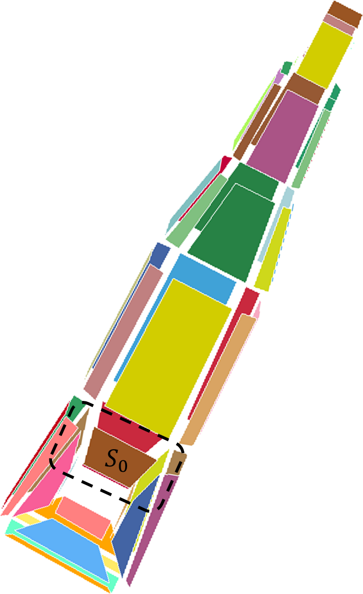
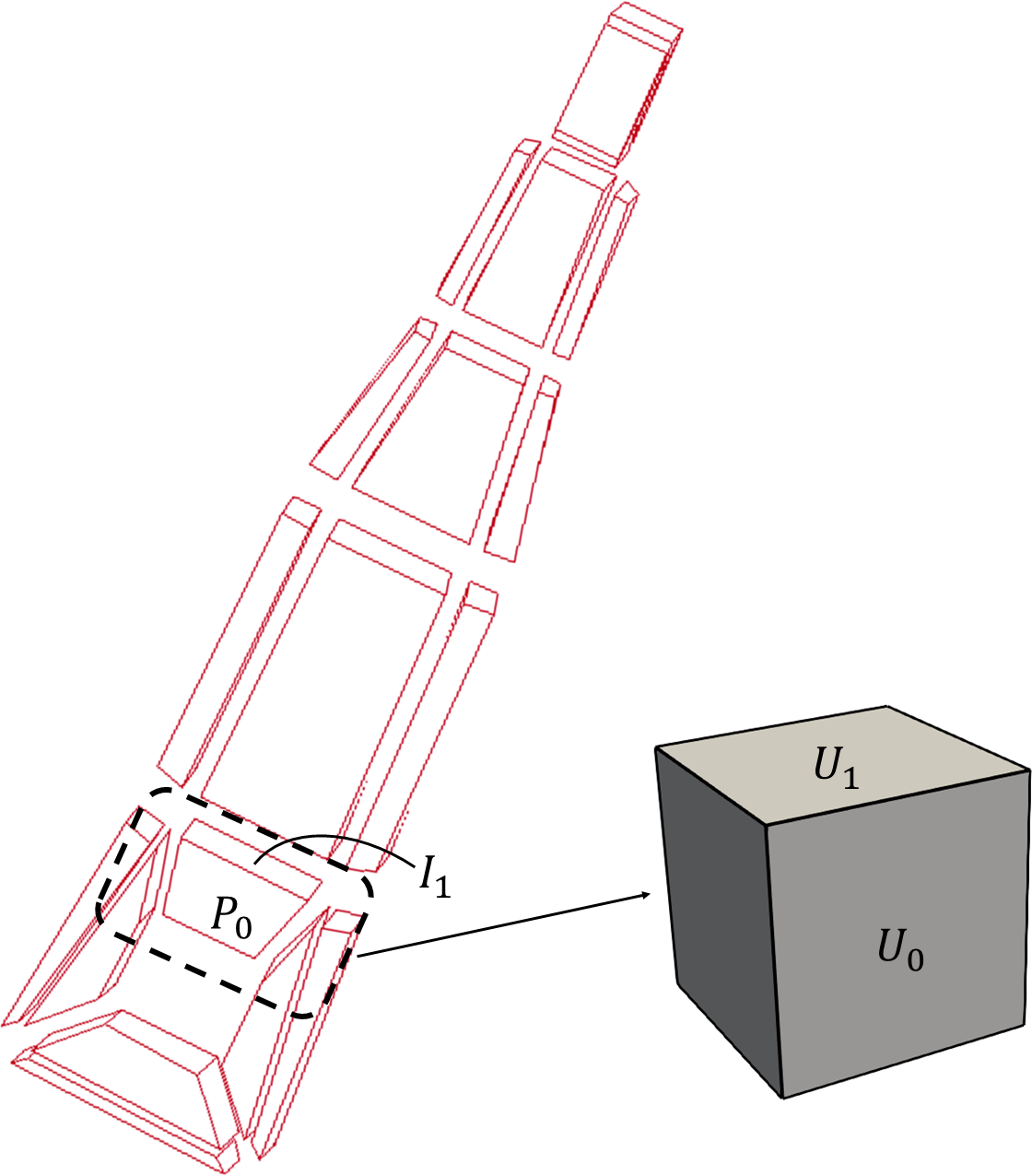
(a)	(b)

Figure 2: The polycube construction and the parametric mapping process. (a) The boundary surface of the polycube generated by Polycube Boundary Surface Construction Algorithm; (b) The interior corners and connectivity manually created in LS-PrePost to generate polycube structure. We split the polycube into multiple cubes and use each individual cube as the parametric domain. $S_{0}$, $P_{0}$ and $U_{0}$ are used for parametric mapping. $I_{1}$ and $U_{1}$ are used for linear interpolation to create interior vertices of the mesh.

3.3 Parametric mapping and octree subdivision

After the polycube is constructed, we need to build a bijective mapping between the input triangle mesh and the boundary surface of the polycube structure. In our software, we implement the same idea as in Liu2015 to use a unit cube as the parametric domain for polycube structure. As a result, we can construct a generalized polycube structure (see Fig. 2(b)) that can align with the given geometry better and generate a high quality hex mesh.

Through the pseudocode in Parametric Mapping Algorithm, we describe how the segmented surface mesh, the polycube structure and the unit cube are combined to create a (volume) parametric mapping and octree subdivision. Let $\{S_{i}\}_{i=1}^{N}$ be the segmented surface patches coming from the segmentation result (see Fig. 2(a)). Each segmented surface patch corresponds to one boundary surface of the polycube $P_{i}$ $(1\leq i\leq N)$ (see Fig. 2(b)), where $N$ is the number of the boundary surface. There are also interior surfaces, denoted by $I_{j}$ $(1\leq j\leq M)$, where $M$ is the number of the interior surface. The union of $\{P_{i}\}_{i=1}^{N}$ and $\{I_{j}\}_{j=1}^{M}$ is the set of surfaces of the polycube structure. For the parametric domain, let $\{U_{k}\}_{k=1}^{6}$ denote the six surface patches of the unit cube (see Fig. 2(b)).

Each cubic region in the polycube structure represents one volumetric region of the geometry and has a unit cube as its parametric domain. Fig. 2(b) shows the example of one cubic region and its corresponding volume domain of the geometry marked in the dashed rectangle. Therefore, for each cube in the polycube structure, we can find its boundary surface $P_{i}$ and map the segmented surface patch $S_{i}$ to its corresponding parametric surface $U_{k}$ of the unit cube. To map $S_{i}$ to $U_{k}$, we first map its corresponding boundary edges of $S_{i}$ to the boundary edges of $U_{k}$. Then we get the parameterization of $S_{i}$ by using the cotangent Laplace operator to compute the harmonic function wenyan2011b ; eck1995multiresolution . Note that for an interior surface $I_{j}$ of the polycube structure, we skip the parametric mapping step.

An all-hex mesh can be obtained from this surface parameterization combined with the octree subdivision. We generate the hex element for each cubic region in the following process. To obtain vertex coordinates on the segmented patch $S_{i}$, we first subdivide the unit cube (see Fig. 2(b)) recursively to get their parametric coordinates. The physical coordinates can be obtained by using the parametric mapping, which has a one-to-one correspondence between the parametric domain $U_{k}$ and the physical domain $S_{i}$. To obtain the vertices on the interior surface of the cubic region, we skip the parametric mapping step and directly use the linear interpolation to calculate the physical coordinates. Fig. 2 shows the example of the rod model. A composition of mappings among $S_{0}$, $P_{0}$ and $U_{0}$ is done to build parametric mapping and obtain vertex coordinates on the surface $S_{0}$. $I_{1}$ and $U_{1}$ are combined for linear interpolation to obtain the vertices on the interior surface of the cubic region. Finally, the vertices inside the cubic region are calculated by linear interpolation. The entire all-hex mesh is built by going through all the cubic regions.

Based on Parametric Mapping Algorithm, we implement and organize the code into a CLI program ( ParametricMapping.exe) that can generate an all-hex mesh by combining parametric mapping with the octree subdivision. Here, we run the following command to generate an all-hex mesh for the rod model:

⬇

1ParametricMapping.exe -i rod_indexPatch_read.k -p

2rod_polycube_structure.k -o rod_hex.vtk -s 2

There are three options used in the command:

• -i: Surface triangle mesh of the input geometry with segmentation information (rod_indexPatch_read.k);

• -o: Unstructured hex mesh (rod_hex.vtk);

• -p: Polycube structure (rod_polycube_structure.k); and

• -s: Octree level.

We use -i to set the segmentation file generated in Section 3.1 and use -p to set the polycube structure created in Section 3.2. Option -s is used to set the level of recursive subdivision to be applied. There is no subdivision if we set -s to be 0. In the rod model, we set -s to be 2 to create a level-2 all-hex mesh. The output all-hex mesh is stored in the VTK format (see Fig. 1(g)) and it can be visualized in Paraview ahrens2005paraview .

Parametric Mapping Algorithm

1:Segmented triangle mesh $\mathcal{T}=\{S_{i}\}_{i=1}^{N}$, polycube structure

2:All-hex mesh

3:Find boundary surfaces $\{P_{i}\}_{i=1}^{N}$ and interior surfaces $\{I_{j}\}_{j=1}^{M}$ in the polycube structure

4:

5:for each cube in the polycube structure do

6:     Create a unit cube $\{U_{k}\}_{k=1}^{6}$ as the parametric domain

7:     for each surface in the cube do

8:         if it is a boundary surface $P_{i}$ then

9:              Get the surface parameterization $f:S_{i}\to U_{k}\subset\mathbb{R}^{2}$

10:         end if

11:     end for

12:end for

13:

14:for each cube in the polycube structure do

15:     Subdivide the unit cube $\{U_{k}\}_{k=1}^{6}$ recursively to get parametric coordinates $v_{{}_{para}}$

16:     for each surface in the cube do

17:         if it is a boundary surface $P_{i}$ then

18:              Obtain physical coordinates using $f^{-1}(v_{{}_{para}})$

19:         else if it is an interior surface $I_{j}$ then

20:              Obtain physical coordinates using linear interpolation

21:         end if

22:     end for

23:     Obtain interior vertices in the cubic region using linear interpolation

24:end for

25:Combine hex elements from each cubic region

3.4 Quality improvement

If the quality of the hex mesh is not satisfactory, quality improvement needs to be applied to the hex mesh. We integrate three quality improvement techniques in the software package, namely pillowing, smoothing and optimization. Users can improve mesh quality through the command line options before building volumetric splines.

We first use pillowing to insert one layer around the boundary wenyan2011b . By using the pillowing technique, we ensure that each element has at most one face on the boundary, which can help improve the mesh quality around the boundary. After pillowing, smoothing and optimization wenyan2011b are used to further improve mesh quality. For smoothing, different relocation methods are applied to three types of vertices: vertices on sharp edges on the boundary, vertices on the boundary surface, and interior vertices. For each sharp-edge vertex, we first detect its two neighboring vertices on the curve, and then calculate their middle point. For each vertex on the boundary surface, we calculate the area center of its neighboring boundary quadrilaterals (quads). For each interior vertex, we calculate the weighted volume center of its neighboring hex elements as the new position. We relocate a vertex in an iterative way. Each time the vertex moves only a small step towards the new position and this movement is done only if the new location results in an improved local Jacobian.

If there are still poor quality elements after smoothing, we run the optimization whose objective function is the Jacobian. Each vertex is then moved toward an optimal position that maximizes the worst Jacobian. We present Quality Improvement Algorithm for quality improvement. Here, we show how to improve mesh quality for the rod model. We first run the following command to perform pillowing on the rod model:

⬇

1Quality.exe -i rod_hex.vtk -Q -m 1 -n 1 -o rod_hex_pillow.vtk

There are four options used in the command:

• -i: Unstructured hex mesh (rod_hex.vtk);

• -o: The hex mesh after quality improvement (rod_hex_pillow.vtk);

• -m: Improvement method. Pillowing when -m 1; and

• -n: Number of pillowing layer.

Option -n allows users to specify the number of layers to be inserted. With -n 1, we insert one layer around the boundary, which is enough to ensure each element have at most one face on the boundary. The result is shown in Fig. 3(a).

After pillowing, we can use the following command to smooth the mesh:

⬇

1Quality.exe -i rod_hex_pillow.vtk -Q -m 2 -p 0.001 -n 50 -s 2 -o rod_hex_pillow_lap.vtk

There are seven options used in the command:

• -i: The input unstructured hex mesh in the vtk format (rod_hex_pillow.vtk);

• -o: The output hex mesh after quality improvement (rod_hex_pillow_lap.vtk);

• -m: Improvement method. Smoothing when -m 2; and

• -s: Sharp feature preservation

  • -s 0: No sharp features are preserved;

  • -s 1: Detect sharp features automatically, and set tolerance -t; and

  • -s 2: Manually select sharp feature points and store the indices in the ”sharp.txt” file.

• -t: Tolerance for automatically detecting sharp features;

• -p: Step size for smoothing; and

• -n: Number of steps for smoothing.

By using the above command, we relocate a vertex only if the new location will improve the local scaled Jacobian. Option -s is used to preserve sharp features. Here, sharp feature detection is only based on the mesh normal information. Therefore, it is not robust for complex geometries and manual work is needed to adjust sharp features. When we use automatic detection with option -s 1, we need to set a tolerance -t. There is no typical number for this option. We need to do a trial and error to get the optimal value. For the rod model, we set it to be 0.8. However, some sharp features may not be detected regardless of the tolerance. User intervention is needed with the option -s 2 if automatic detection is not satisfactory. Through this command line option, Quality.exe will read an input file that includes the user-defined sharp features. The snippets of the related file is shown in Appendix A5.

Then we run the optimization step by using the command:

⬇

1Quality.exe -i rod_hex_pillow_smooth.vtk -Q -m 3 -p 0.001 -n 15 -o rod_hex_pillow_smooth_opt.vtk

There are five options used in the command:

• -i: Unstructured hex mesh (rod_hex_pillow_smooth.vtk);

• -o: The hex mesh after quality improvement (rod_hex_pillow_smooth_opt.vtk);

• -t: Tolerance related to sharp feature preservation;

• -m: Improvement method. Optimization when -m 3;

• -p: Step size for optimization; and

• -n: Number of steps for optimization.

The quality improvement result for the rod model is shown in Fig. 3 with a boundary layer created using pillowing, followed up by smoothing and optimization.

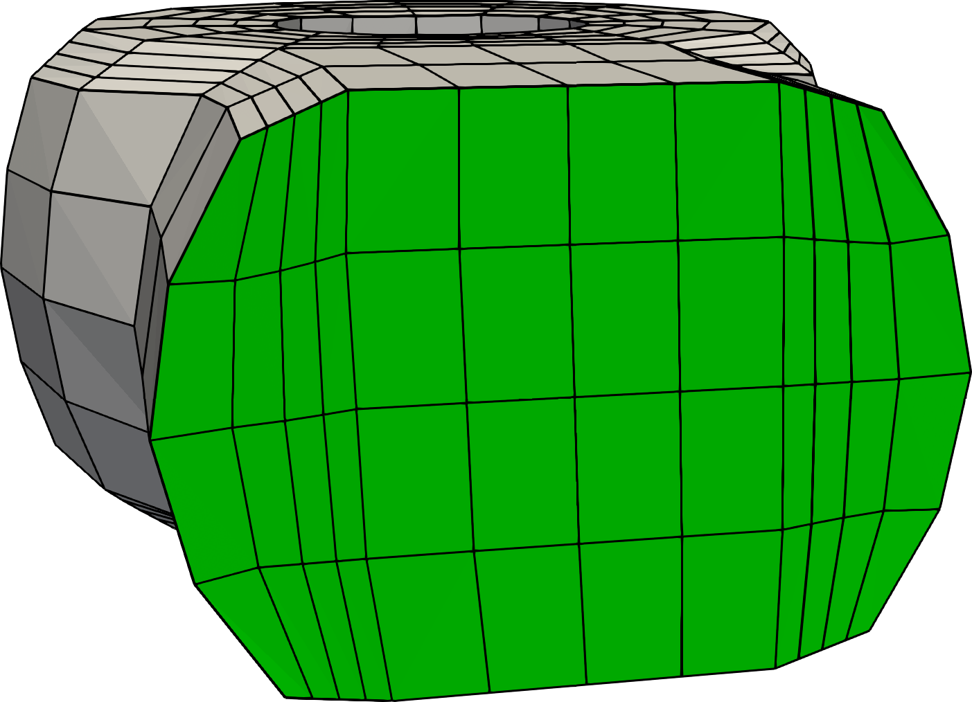
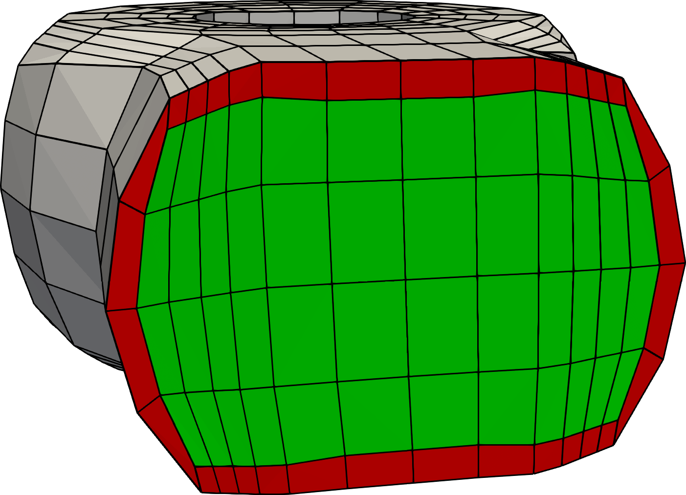
(a)		(b)

Figure 3: Mesh quality improvement. (a) The original mesh before quality improvement; (b) The mesh after pillowing, smoothing and optimization. Part of the mesh is removed to show the interior. The elements on the original cross section are labeled in green color while the inserted boundary layer is labeled in red color.

Quality Improvement Algorithm

1:Hex mesh, step number $n$

2:Hex mesh with improved quality

3:

4:Insert an outer layer to the input mesh

5:

6:while  iteration ¡ $n$ do

7:     for each vertex $v_{i}$ do

8:         if $v_{i}$ is on a sharp edge then

9:              if  improving the local Jacobian then

10:                  Relocate $v_{i}$ a small step towards the middle of its neighboring vertices

11:              end if

12:         else if $v_{i}$ is on the boundary surface then

13:              if  improving the local Jacobian then

14:                  Relocate $v_{i}$ a small step towards the the area center of its neighboring boundary quads

15:              end if

16:         else if $v_{i}$ is an interior vertex  then

17:              if  improving the local Jacobian then

18:                  Relocate $v_{i}$ a small step towards the weighted volume center of its neighboring elements

19:              end if

20:         end if

21:     end for

22:end while

23:

24:while  iteration ¡ $n$ do

25:     for each negative Jacobian element do

26:         if  improving the local Jacobian then

27:              Relocate $v_{i}$ to maximize the Jacobian

28:         end if

29:     end for

30:     Relocate vertices where Jacobian is minimum to maximize the worst Jacobian

31:end while

4 Hex2Spline: Unstructured spline construction

With the generated hex mesh as the input control mesh, now we present the Hex2Spline software package to build TH-spline3D. TH-spline3D can define spline functions on arbitrarily unstructured hex meshes. It further supports local refinement for adaptive IGA. Hex2Spline can output the Bézier information of constructed volumetric splines, which can be easily used in LS-DYNA or any other existing IGA frameworks. In the following, we introduce the main algorithm for each component of the Hex2Spline software package, including blending functions on an unstructured hex mesh, TH-spline3D with local refinement, and Bézier extraction.

4.1 Blending functions on an unstructured hex mesh

In this section, we describe how to build blending functions on an all-hex mesh. Hex2Spline supports arbitrarily unstructured all-hex mesh. In the following, we denote $\Omega_{e}$ as an hex element indexed by $e$. There are three types of elements in the hex mesh: boundary elements, interior regular elements and interior irregular elements. The element is defined as a boundary element if it contains a boundary vertex; otherwise, it is an interior element. For an interior element, if it contains an extraordinary edge, we call it an irregular element; otherwise, it is a regular element. In the following, we discuss the main algorithm for building blending functions on boundary elements and interior irregular elements. A regular interior element is a special case of an irregular interior element whose blending functions are merely tricubic B-splines. Note that the following construction only applies to tricubic splines with uniform knot intervals (i.e., the same knot interval for every edge).

Blending Functions Algorithm (Interior) shows the pseudocode to obtain the blending functions defined on an interior irregular element. They are obtained through the Bézier extraction matrix $\mathbf{M}$. $\mathbf{M}$ can be obtained by computing the 64 Bézier control points $\mathbf{Q}_{e}$ from a local spline control mesh $\mathcal{N}$ that consists of $\Omega_{e}$ and its one-ring neighborhood. Each of these Bézier points is obtained by a convex combination of the vertices in the local control mesh, and we have $\mathbf{Q}_{e}=\mathbf{M}\mathbf{P}$, where $\mathbf{P}$ is the vector of vertices in the local control mesh. Then the blending functions on $\Omega_{e}$ are defined by using the transpose of $\mathbf{M}$, that is, $\mathbf{B}_{e}=\mathbf{M}^{T}\mathbf{b}$, where

$$\mathbf{b}= [N_{0}(u)N_{0}(v)N_{0}(w),\ldots,N_{0}(u)N_{1}(v)N_{0}(w),N_{1}(u)N_{1}(v)N_{0}(w),$$

$$\ldots,N_{0}(u)N_{0}(v)N_{1}(w),N_{1}(u)N_{0}(v)N_{1}(w),\ldots,N_{3}(u)N_{3}(v)N_{3}(w)]^{T},$$

is the vector of 64 tricubic Bernstein polynomials. Each univariate cubic Bernstein polynomial is given as $N_{k}(t)=\dbinom{3}{k}(1-t)^{3-k}t^{k}$ ($k=0,\ldots,3$). Readers can refer to wei17a for the coefficients of $\mathbf{M}$. Note that we only need $\mathbf{M}$ to define $\mathbf{B}_{e}$, and we do not actually compute Bézier points.

Blending Functions Algorithm (Interior)

1:An interior element $\Omega_{e}$ and its local control mesh $\mathcal{N}$

2:The blending functions $\mathbf{B}_{e}$

3:

4:for each Bézier point $Q_{e,i}$ of $\Omega_{e}$, where $i=0,\ldots,63$ do

5:     if  $Q_{e,i}$ is body point then

6:         Compute its coordinates based on $\mathbf{P}$

7:     else if  $Q_{e,i}$ is face, edge, corner point then

8:         Compute its coordinates by averaging the nearest body points

9:     end if

10:end for

11:Ensemble matrix $\mathbf{M}$ such that $\mathbf{Q}_{e}=\mathbf{M}\mathbf{P}$

12:

13:$\mathbf{B}_{e}=\mathbf{M}^{T}\mathbf{b}$

Blending Functions Algorithm (Boundary) shows the pseudocode to define blending functions on a boundary element. The body Bézier points and the Bézier points on the interior corners, edges or faces are obtained the same way as in Blending Functions Algorithm (Interior), while the Bézier points on the boundary is defined using only the boundary quadrilateral mesh. The 16 Bézier points on a boundary face can be obtained by convex combinations of the vertices on the local quad control mesh. The detailed computation method is explained in wei17a . We finally get all the Bézier points as $\mathbf{Q}_{e}=\mathbf{M}\mathbf{P}$. The blending functions are then defined by $\mathbf{B}_{e}=\mathbf{M}^{T}\mathbf{b}$. Note that Blending Functions Algorithm (Boundary) can also be used to preserve sharp features in the mesh by adjusting the Bézier extraction matrix $\mathbf{M}$. Reader can refer to wei17a for details.

Blending Functions Algorithm (Boundary)

1:A boundary element $\Omega_{e}$ and its local control mesh $\mathcal{N}$; sharp feature information

2:The blending functions $\mathbf{B}_{e}$

3:

4:for each Bézier point $Q_{e,i}$ of $\Omega_{e}$, where $i=0,\ldots,63$ do

5:     if $Q_{e,i}$ corresponds to a sharp corner $P_{k}$ then

6:         $Q_{e,i}=P_{k}$

7:     else if  $Q_{e,i}$ is on a sharp edge then

8:         Compute its coordinates as a convex combination of the two end points of the sharp edge

9:     else if  $Q_{e,i}$ is on the boundary then

10:         if  $Q_{e,i}$ is a face point then

11:              Compute its coordinates based on $P_{k}$

12:         else if  $Q_{e,i}$ is an edge or a corner point then

13:              Compute its coordinates by averaging the nearest boundary face points

14:         end if

15:     else if  $Q_{e,i}$ is a body point or on an interior surface then

16:         Calculate $Q_{e,i}$ the same as Blending Functions Algorithm (Interior)

17:     end if

18:end for

19:Ensemble matrix $\mathbf{M}$ such that $\mathbf{Q}_{e}=\mathbf{M}\mathbf{P}$

20:

21:$\mathbf{B}_{e}=\mathbf{M}^{T}\mathbf{b}$

4.2 TH-spline3D for local refinement

The next step is to introduce local refinement to achieve computational efficiency and accuracy. TH-spline3D employs a hierarchical structure and uses the truncation mechanism to perform local refinement. Global refinement is also supported since it is a special case of local refinement, and it is done by Catmull-Clark subdivision for solids ref:bajaj02 ; ref:burkhart10 .

TH-spline3D Algorithm shows the pseudocode to construct TH-spline3D based on the blending functions developed in Section 4.1. Locally refined meshes as well as spline functions between different levels are related through Catmull-Clark subdivision for solids.

The program allows users to specify a list of target elements to be locally refined. This is enabled by reading a series of user-defined files to the program, each of which contains indices of target elements at a certain level. The input mesh is treated as the level-0 mesh by default, one needs to provide a file named ”lev_rfid.txt” to refine certain level-0 elements. As a result, a level-1 mesh is generated that can be used to define multi-level local refinement. One can check the hierarchical control meshes and add more elements in the ”lev_rfid.txt” file to further refine the mesh.

The remaining procedure to construct TH-spline3D is automatic and can be divided into three steps: i) refine target elements by Catmull-Clark subdivision for solids, ii) select certain blending functions from hierarchical meshes, and iii) truncate some blending functions on the coarse mesh. Then with the help of Blending Functions Algorithm (Interior) and Blending Functions Algorithm (Boundary), we can construct TH-spline3D on hierarchical control meshes. Readers can refer to wei17a for details.

TH-spline3D Algorithm

1:Initial control points $\mathbf{P}^{0}$ and their associated blending functions $\mathcal{B}^{0}$, element $\Omega_{e}$ and its local control mesh $\mathcal{N}$

2:The truncated blending functions $\mathcal{B}_{\text{TH-spline3D}}$

3:

4:if local refinement is needed then

5:     Generate mesh $\mathcal{M}^{\ell+1}$ from mesh $\mathcal{M}^{\ell}$ based on Catmull-Clark subdivision ref:bajaj02 ; ref:burkhart10

6:end if

7:Ensemble matrix $\mathbf{C}$ so that $\mathbf{P}^{\ell+1}=\mathbf{C}\mathbf{P}^{\ell}$

8:

9:Compute the Bézier control points on hierarchical structure $\mathbf{Q}^{\ell+1}=\mathbf{M}\mathbf{\mathbf{P}^{\ell+1}}$

10:Construct the hierarchical B-splines on the hierarchical control meshes by using Blending Functions Algorithm (Interior) or Blending Functions Algorithm (Boundary)

11:

12:Select the blending function to be active

13:Truncate chosen blending functions

14:Collect all the blending functions ($\mathcal{B}_{\text{TH-spline3D}}^{\ell+1}$) up to Level $\ell+1$

4.3 Bézier extraction for LS-DYNA

After blending functions are defined based on Bernstein polynomials, the Bézier information of the constructed volumetric splines can be written in the BEXT file for LS-DYNA. The program will also output files for the visualization of Bézier mesh in Paraview ahrens2005paraview . The BEXT file contains all the control points and the Bézier extraction matrix $\mathbf{M}^{T}$ for each Bézier element. We reduce the file size by using both sparse and dense formats to write $\mathbf{M}^{T}$. The matrix is output row by row. In a sparse format, only non-zeros of a row are output, where an index is paired with each non-zero coefficient to indicate its column location in the matrix. On the other hand, an entire row is output in the dense format without additional column indices. The choice of the two formats depend on the number of non-zeros in a row. The sparse format is favored when the row only has a few non-zeros. The snippets of the BEXT format file is shown in Appendix A6.

4.4 Applying Hex2Spline to the rod model

Based on the above algorithms, we implement and organize the code into a CLI program (Hex2Spline.exe) that can construct TH-spline3D on an unstructured hex mesh and extract Bézier information for analysis. During the spline construction, users can specify if refinement is needed. In the end, Hex2Spline generates the BEXT file for LS-DYNA. The program also supports sharp feature preservation. All the available options for this program are explained as follows:

• -i: Unstructured hex mesh (rod_hex.vtk);

• -o: The BEXT file for LS-DYNA (rod_hex_BEXT.txt);

• -S: Spline construction mode;

• -s: Sharp feature preservation;

  • -s 0: No sharp features need to be preserved;

  • -s 1: Detect sharp feature automatically, and set tolerance -t; and

  • -s 2: Manually select sharp feature points and store them in ”sharp.txt”.

• -g: Set the level of global refinement;

• -l: Enable local refinement; and

• -t: Tolerance related to sharp feature preservation.

Here, we apply local refinement to create a hierarchical mesh of the rod model (see Fig. 1(g)) by using the command:

⬇

1Hex2Spline.exe -i rod_hex.vtk -S -s 2 -l -o rod_hex.BEXT

In the command, we use the option -l to switch on the local refinement mode and construct TH-spline3D with local refinement. Unlike global refinement, users need to prepare a ”lev_rfid.txt” file to specify indices of target elements. Fig. 4(b) shows the spline construction with one level local refinement. Users can perform further refinements level by level. For example, users can edit the ”lev_rfid.txt” file to include more elements and use the same command to perform two levels of local refinement and the result is shown in Fig. 4(c):

⬇

1Hex2Spline.exe -i rod_hex.vtk -S -s 2 -l 2

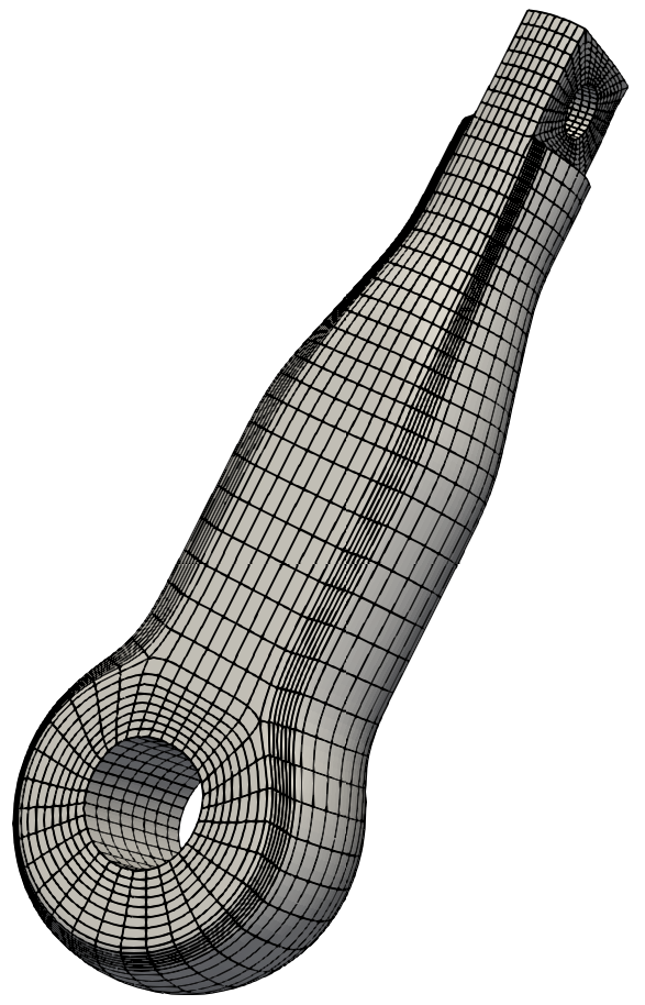
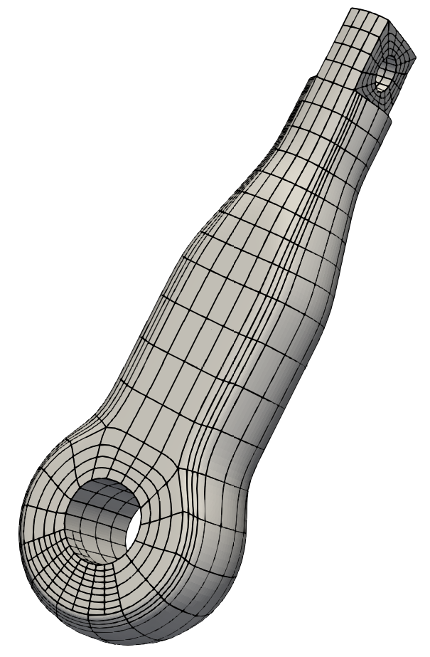
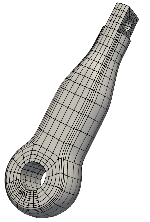
(a)	(b)	(c)

Figure 4: The visualization of the output Bézier mesh with: (a) global refinement; (b) one level local refinement; and (c) two levels of local refinement.

Users can also use the following command to perform spline construction with one level global refinement and the result is shown in Fig. 4(a):

⬇

1Hex2Spline.exe -i rod_hex.vtk -o rod_hex -S -s 2 -g 1

Here we use the option -g to switch on global refinement mode and set the argument to 1 to construct spline with one level global refinement.

5 Applications using HexGen and Hex2Spline

The algorithms discussed in Sections 3 and 4 are implemented in C++. The Eigen library eigenweb and Intel MKL intel-alt are used for matrix and vector operations and numerical linear algebra. We also take advantage of openMP to support multi-threading computation. We use a compiler-independent building system (CMake) and a version-control system (Git) to support software development. We have compiled the source code into two software packages,

• Hex2Gen software package:

  • Segmentation module (Segmentation.exe);

  • Polycube construction module (Polycube.exe);

  • All-hex mesh generation module (ParametricMapping.exe); and

  • Quality improvement module (Quality.exe).

• Hex2Spline software package:

  • Volumetric spline construction module (Hex2Spline.exe).

The software is open-source and can be found in the following Github link (https://github.com/yu-yuxuan/HexGen_Hex2Spline).

We have applied the software packages to several models and generated all-hex meshes with good quality. For each model, we show the HBECVT based segmentation result, further segmentation result, corresponding polycube structure, and the all-hex mesh. These models include: two types of mount and hepta models (Fig. 5); engine mount and lower arm from Honda Co. along with rockerarm (Fig. 6); ant, bust, and fertility models (Fig. 7); and the joint model from Honda Co. (Fig. 8). Table 1 shows the statistics of all testing models. We use the scaled Jacobian to evaluate the quality of all-hex meshes. From Table 1, we can observe that the obtained all-hex meshes have good quality (minimal Jacobian $>$ 0.1). Figs. 5-8(a) show HBECVT segmentation results of testing models, we can observe that the initial segmentation results generated by the HBECVT do not satisfy the topological constraints for polycube construction. We need to further segment each Voronoi region into several patches. The generated polycubes (Figs. 5-8(b)) align with the given geometry better, which in turn induces less mesh distortion and yields a mesh of better quality.

After generating all-hex meshes (Figs. 5-8(c)), we tested all the models for IGA by using TH-spline3D. Bézier elements are extracted for the IGA analysis (Figs. 5-8(d)). For each testing model in Figs. 5-7 , we use LS-DYNA to perform eigenvalue analysis and show the first mode result. For the testing model in Fig. 8, we show the result of solving a Poisson problem in LS-DYNA. From the results we can observe that our algorithm yields valid TH-spline3D for IGA applications in LS-DYNA.

Table 1: Statistics of all the tested models.

Model	Input triangle mesh	Octree	Output hex mesh	Jacobian
	(vertices, elements)	levels	(vertices, elements)	worst
rod (Fig. 1)	(2,238, 4,480)	2	(1,815, 1,280)	0.32
mount1 (Fig. 5)	(886, 1,782)	2	(5,849, 4,480)	0.16
mount2 (Fig. 5)	(895, 1,802)	2	(7,945, 6,208)	0.14
hepta (Fig. 5)	(676, 1,348)	1	(1,259, 944)	0.24
engine mount (Fig. 6)	(57,487, 114,982)	2	(7,338, 5,888)	0.11
lower arm (Fig. 6)	(165,201, 330,410)	1	(1,996, 1,328)	0.10
rockerarm (Fig. 6)	(11,655, 23,310	2	(6,880, 5,696)	0.10
ant (Fig. 7)	(7,216, 14,428)	2	(7,711, 6,176)	0.17
bust (Fig. 7)	(12,596, 25,188)	4	(103,299, 98,816)	0.11
fertility (Fig. 7)	(6,622, 13,256)	2	(4,983, 4,000)	0.20
joint (Fig. 8)	(3,806, 7,612)	2	(7,512, 6,144)	0.10

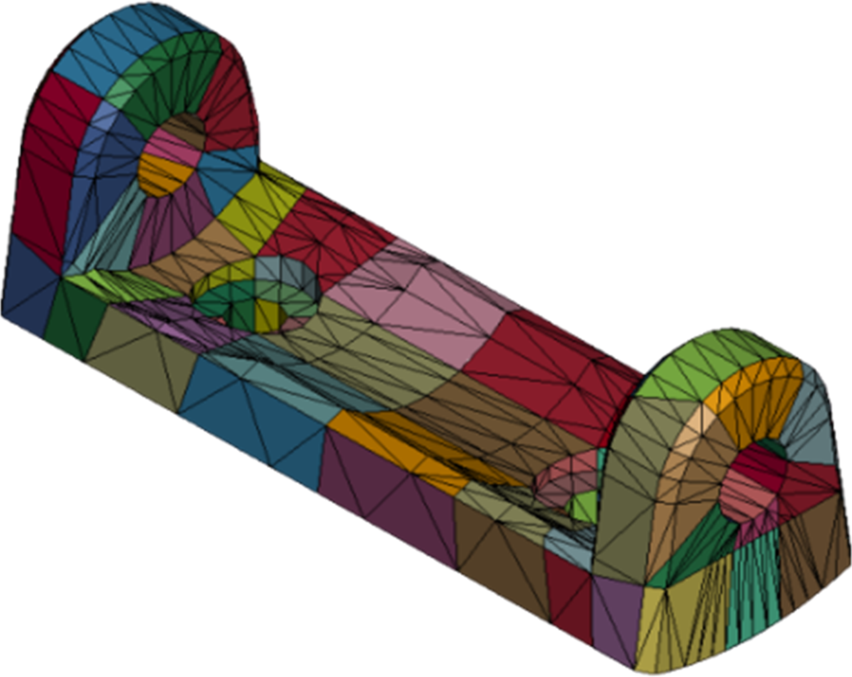
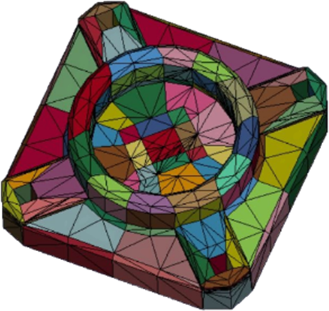
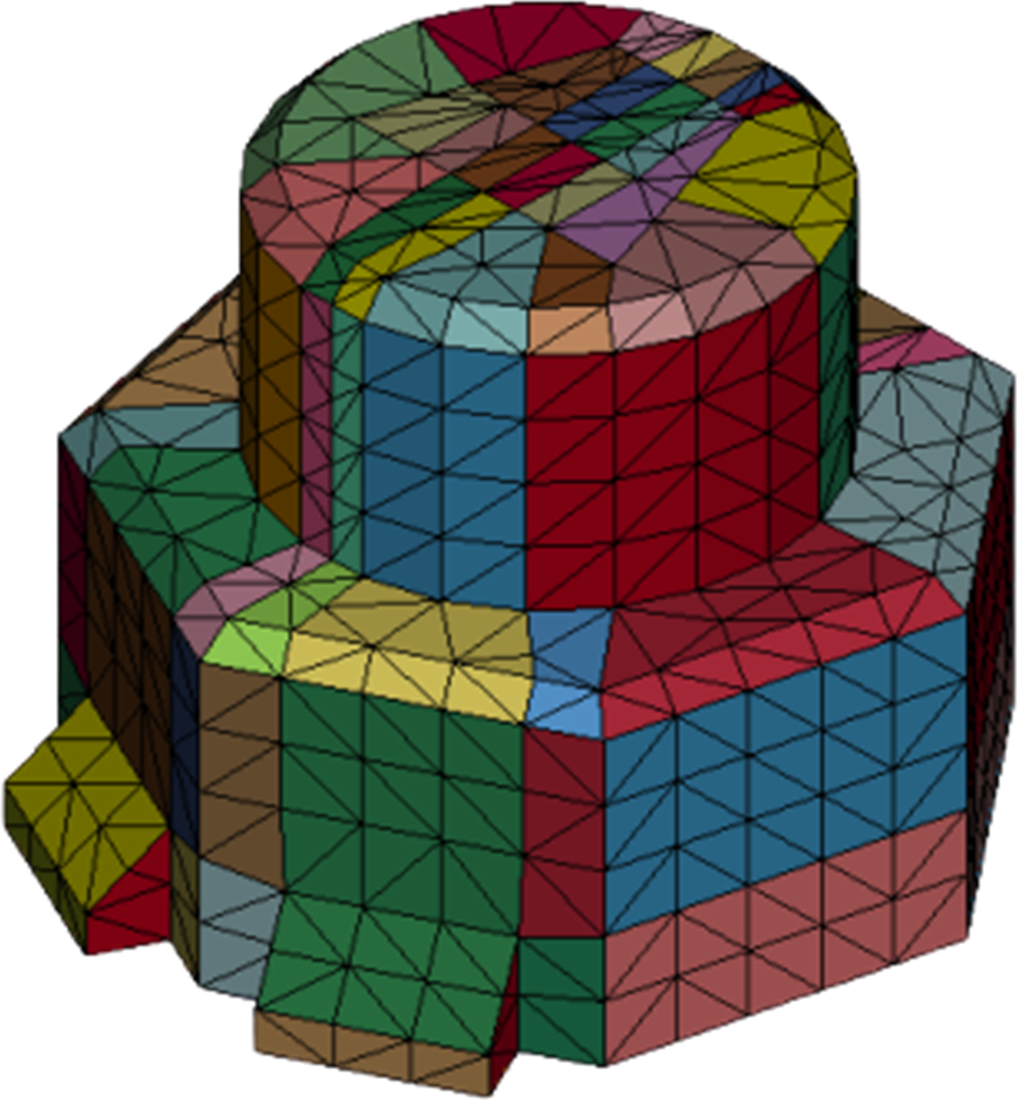
	(a)
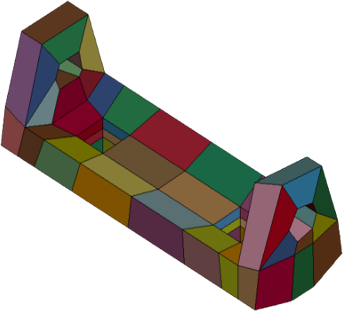
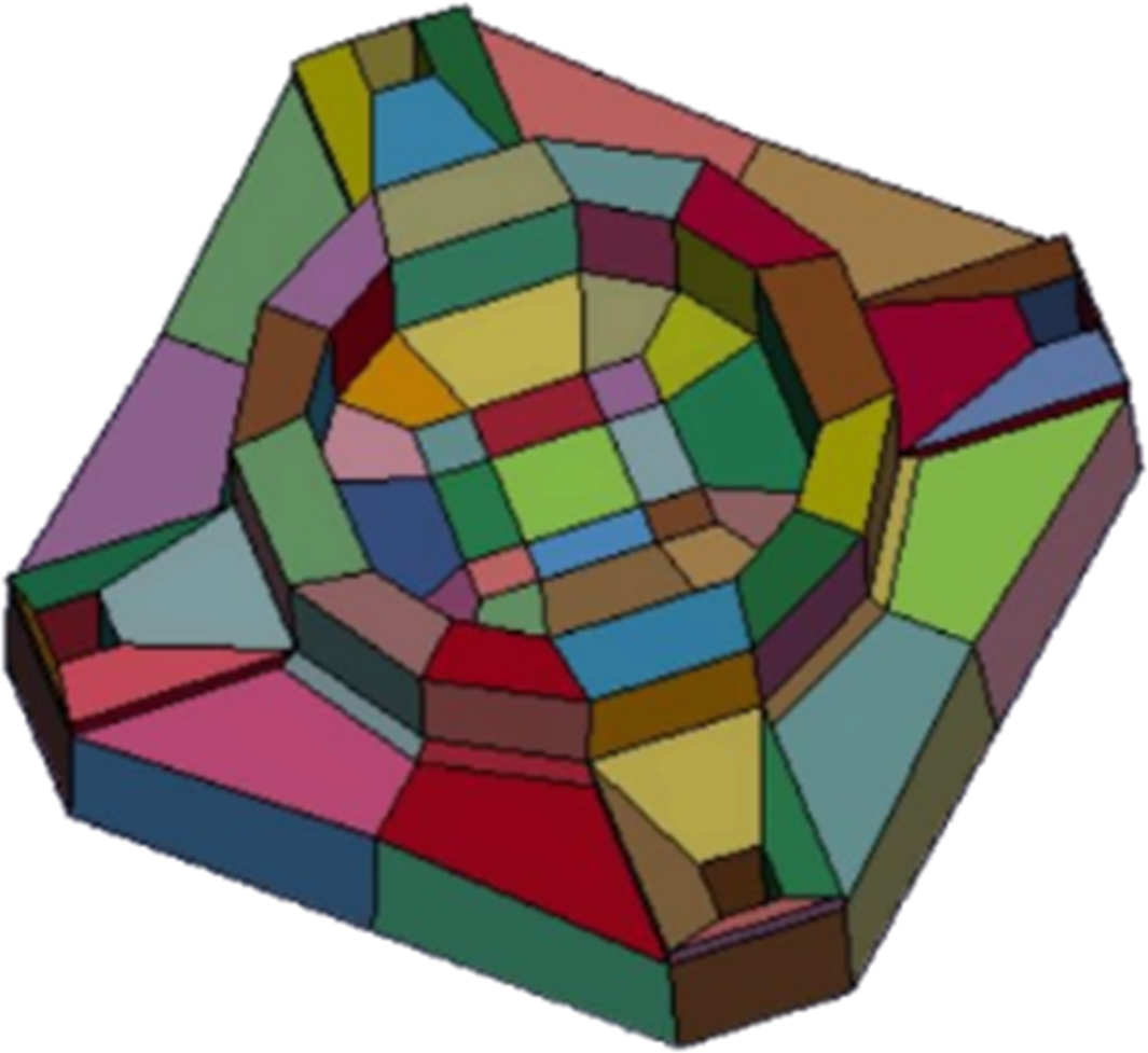
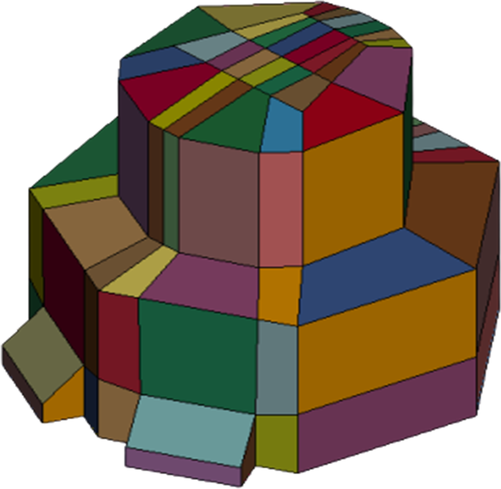
	(b)
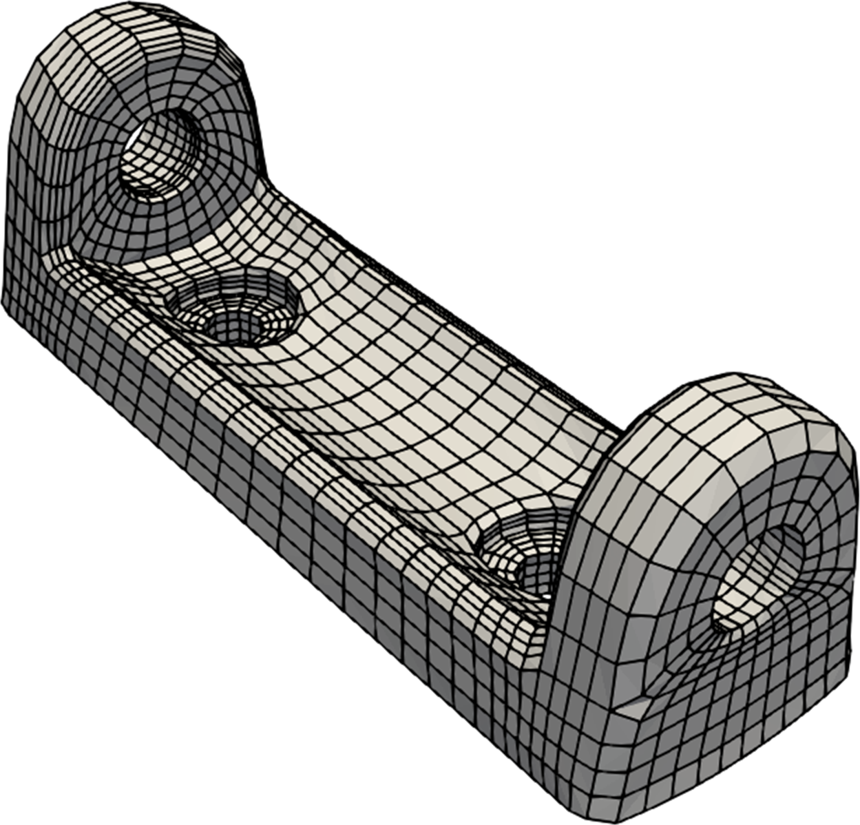
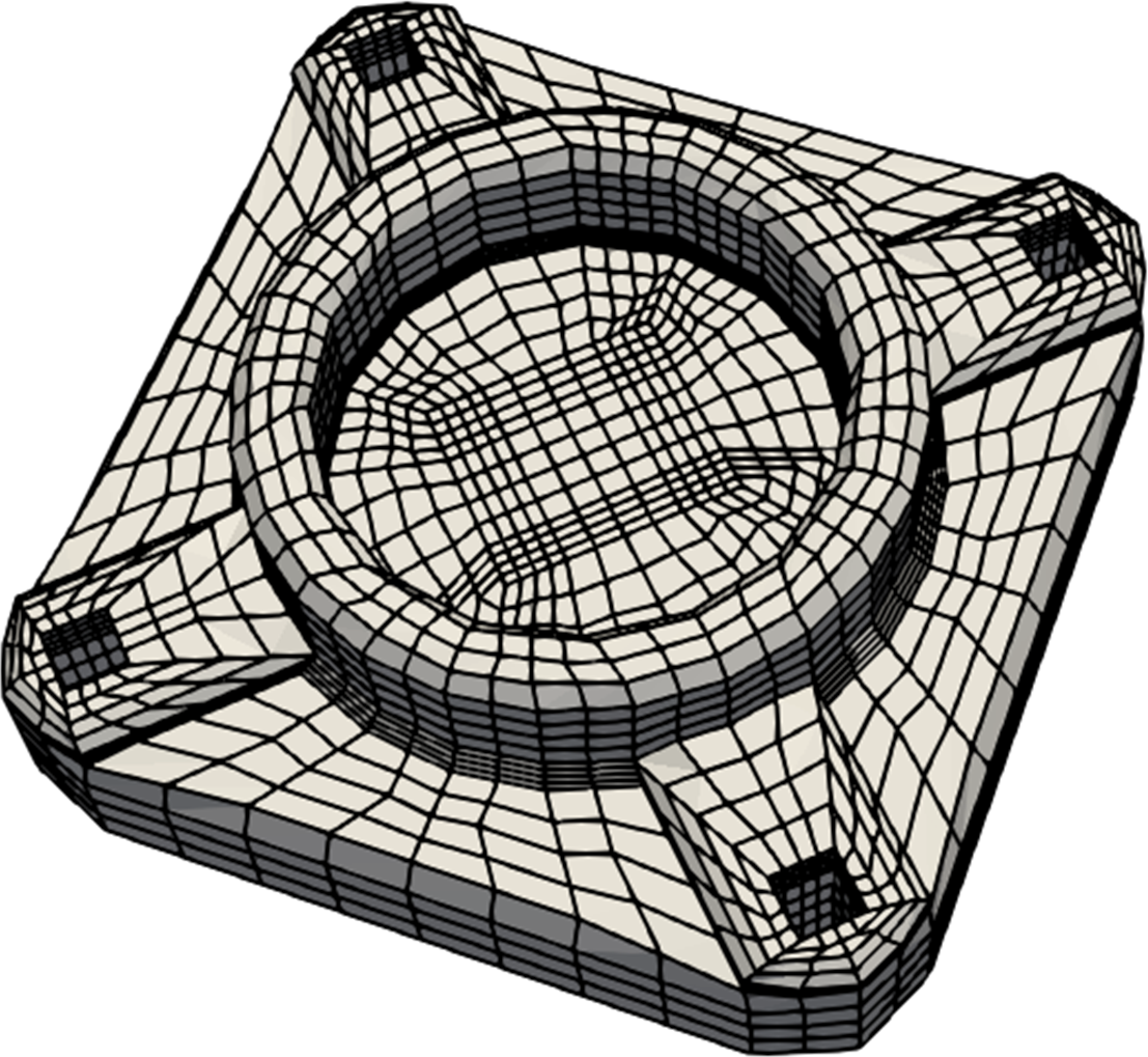
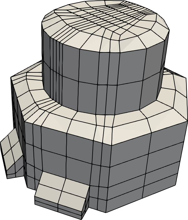
	(c)
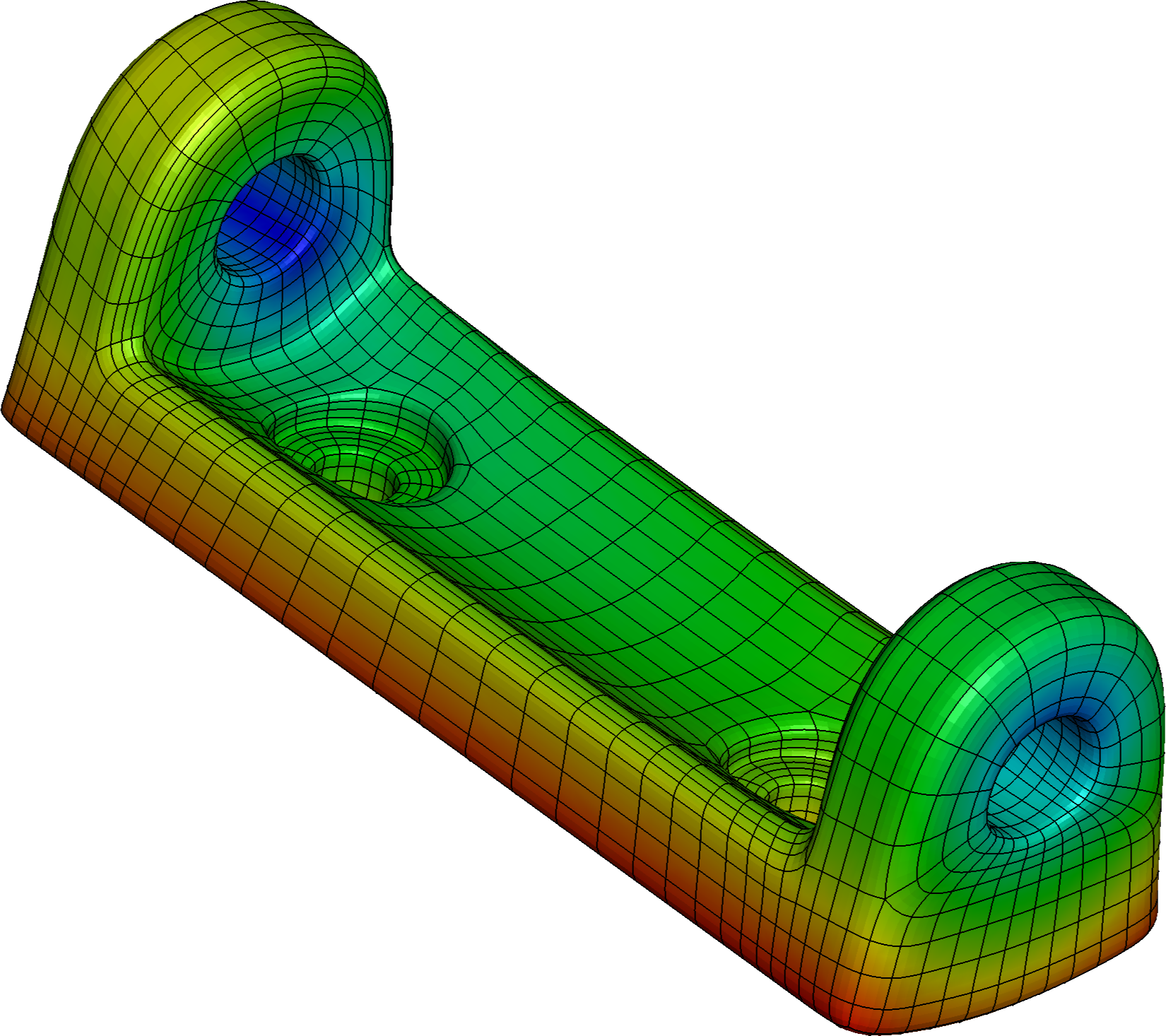
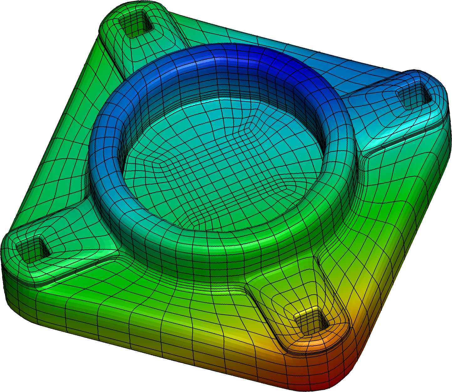
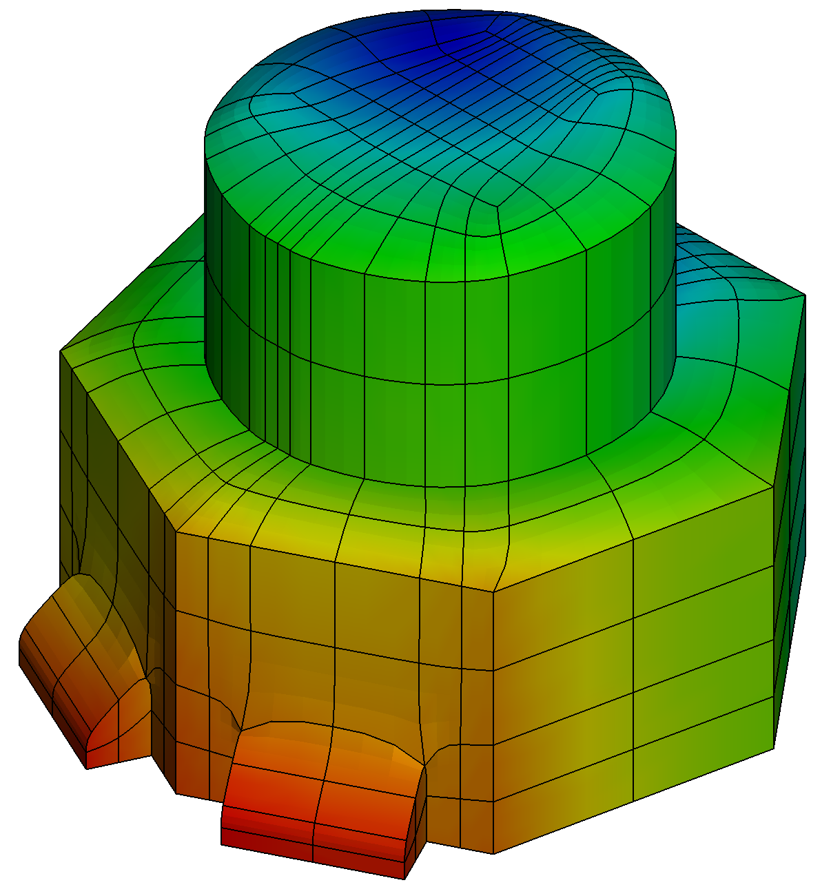
	(d)

Figure 5: Results of two types of mount and hepta models. (a) Surface triangle meshes and segmentation results; (b) Polycube structures; (c) All-hex control meshes; (d) Volumetric splines with IGA results of eigenvalue analysis in LS-DYNA.

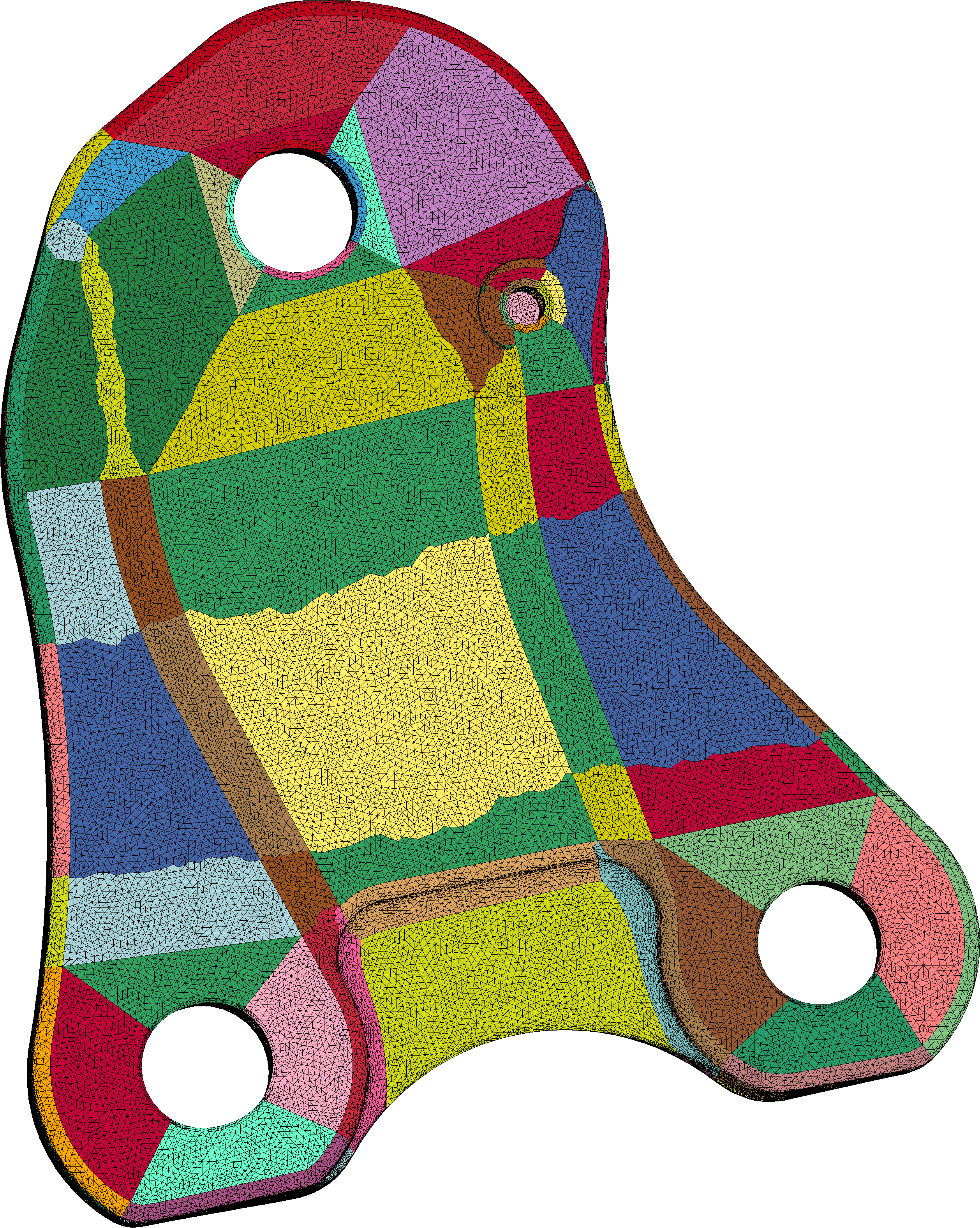
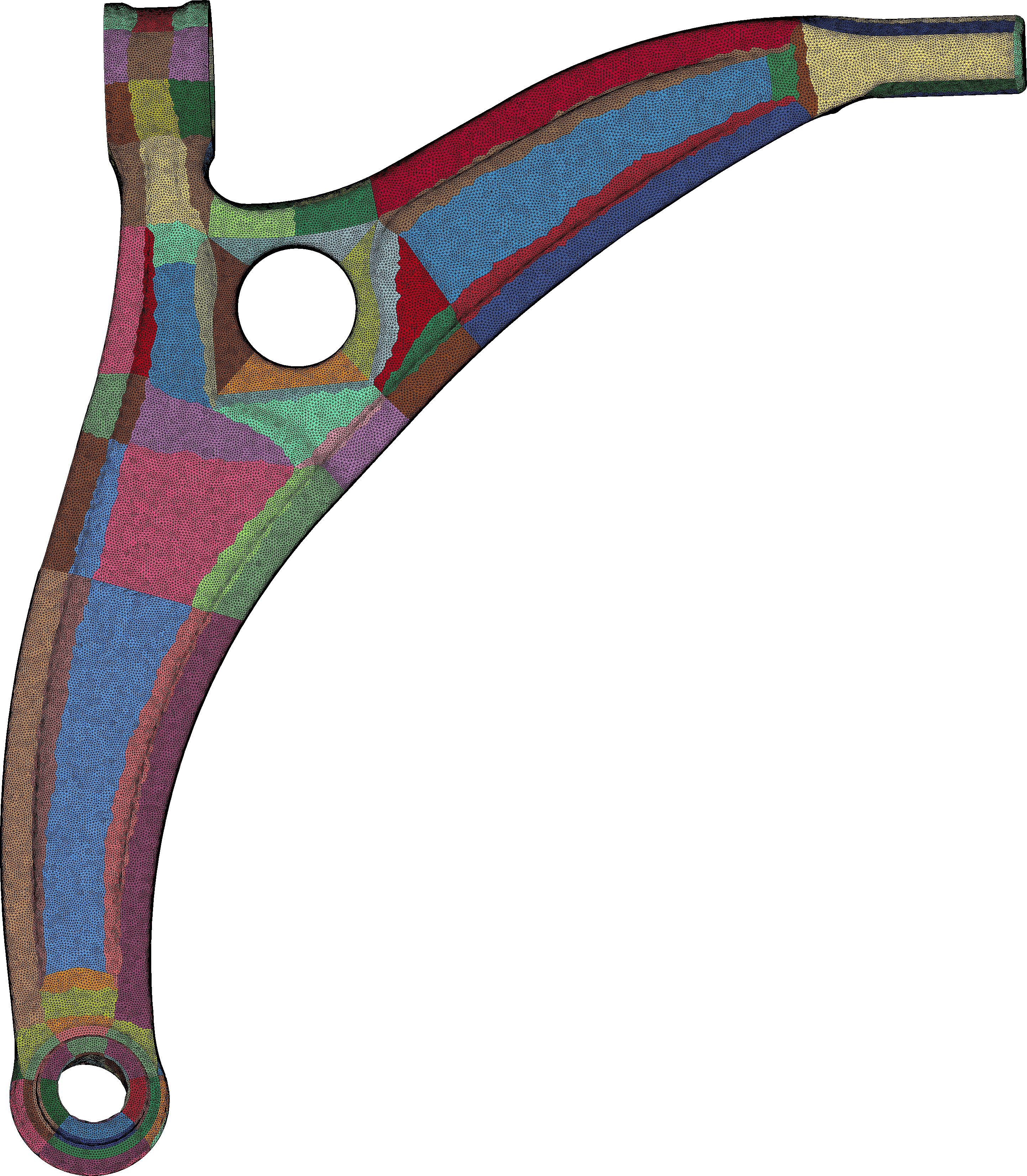
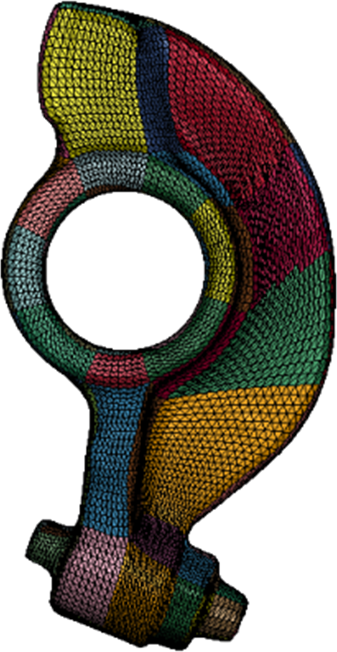
	(a)
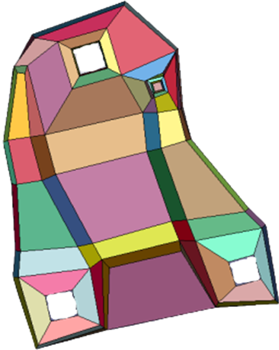
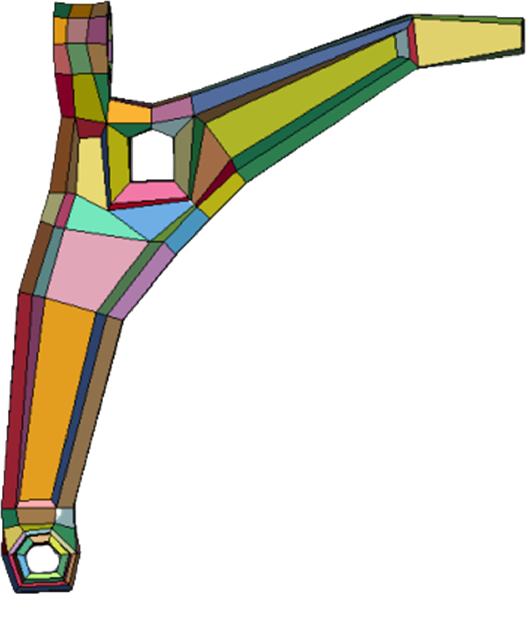
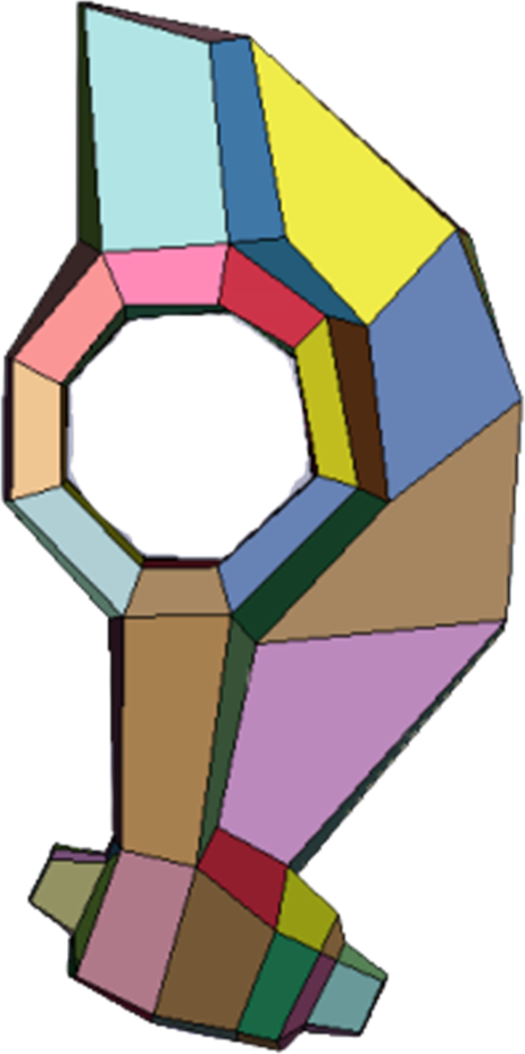
	(b)
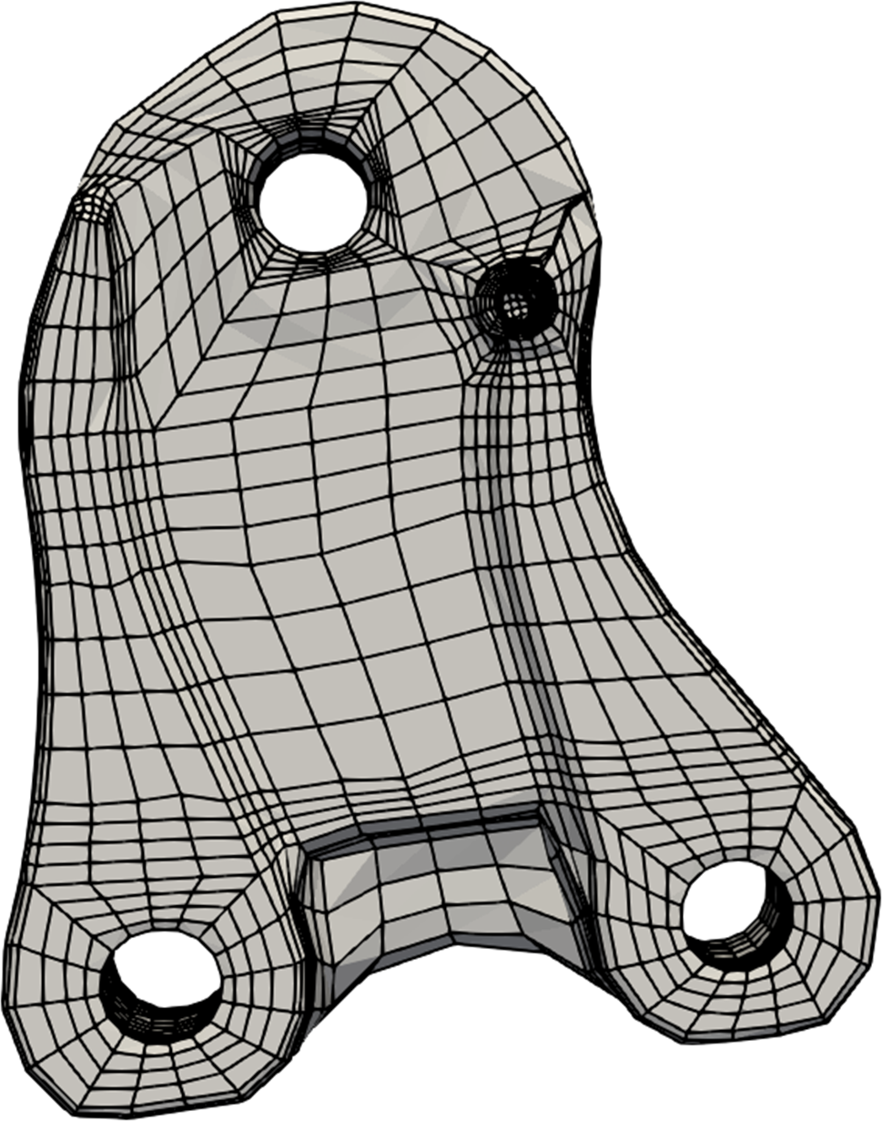
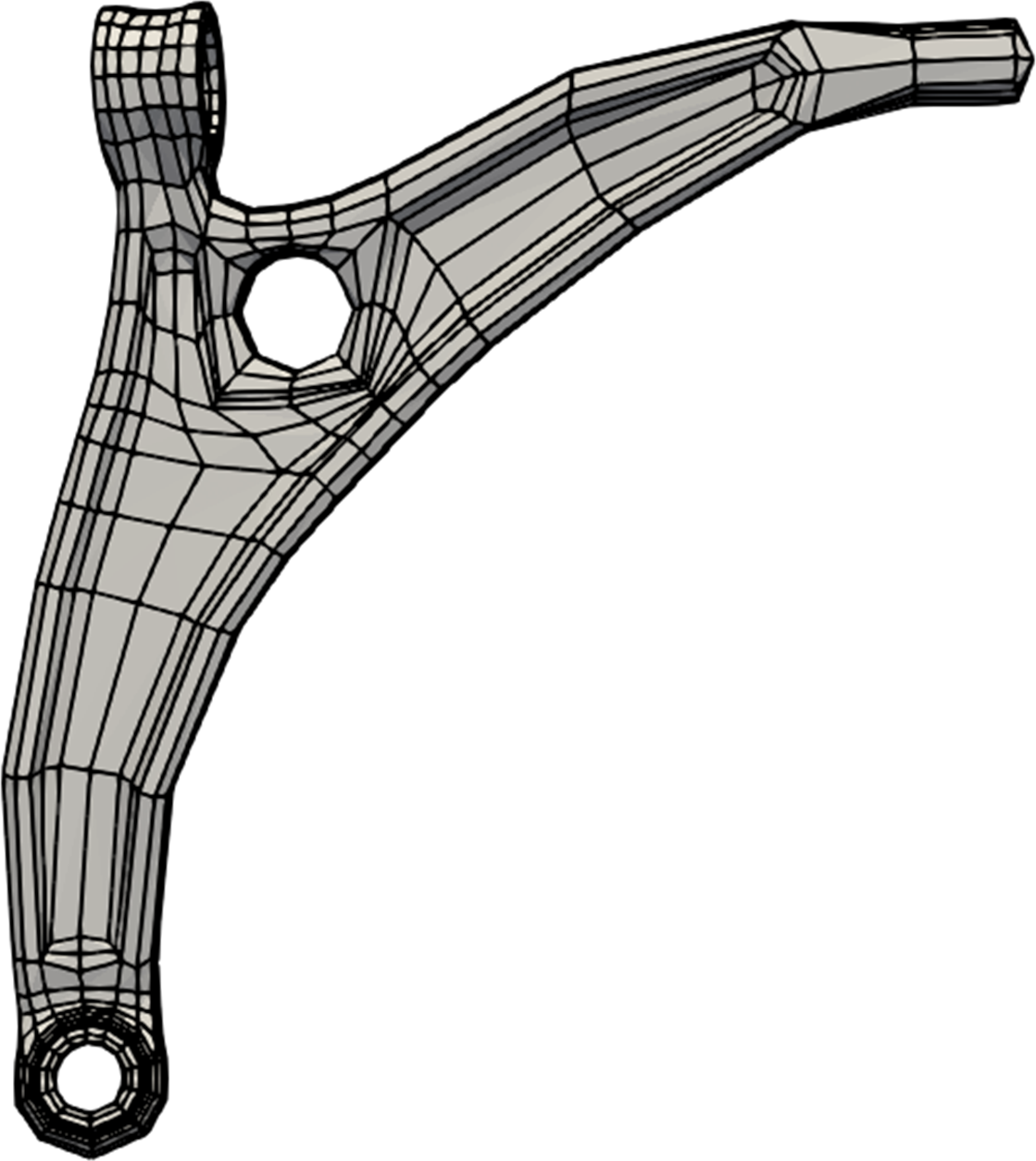
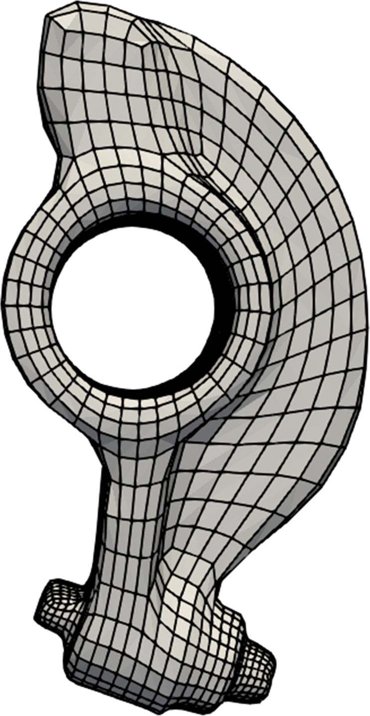
	(c)
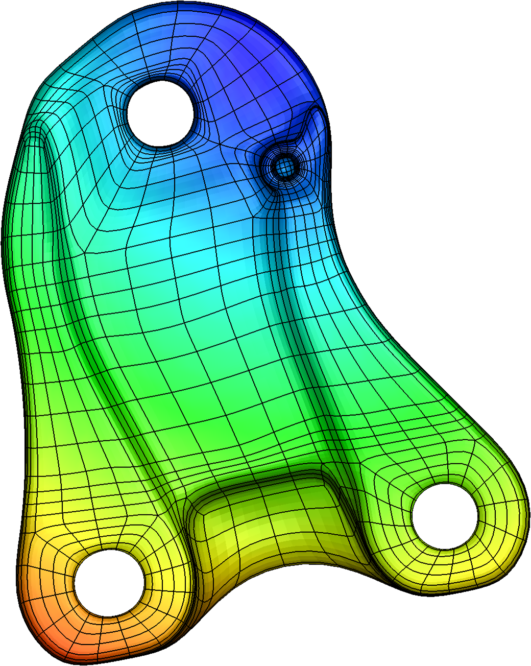
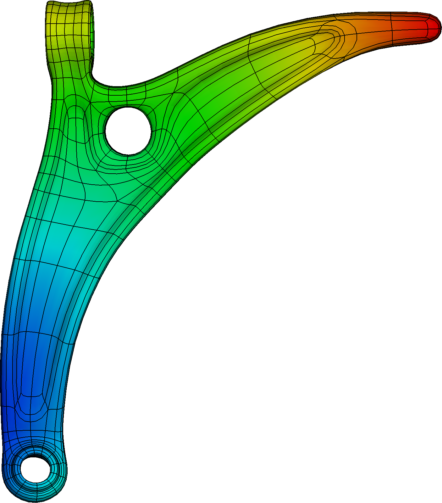
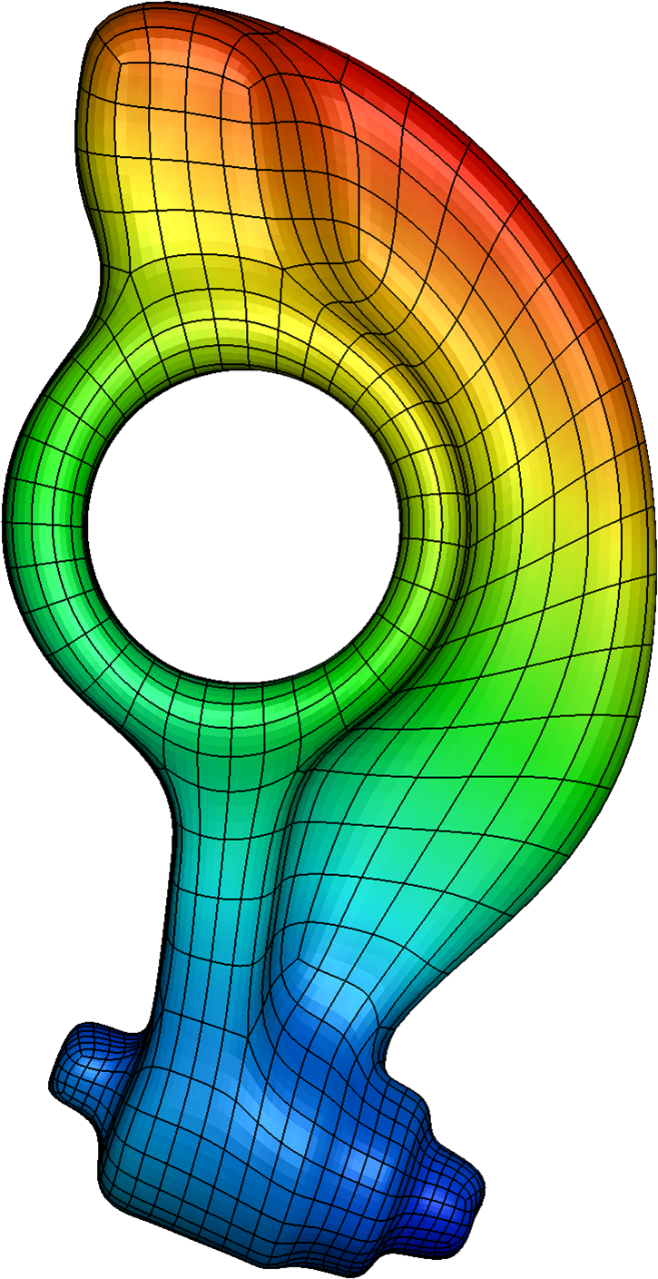
	(d)

Figure 6: Results of engine mount, lower arm, and rockerarm model. (a) Surface triangle meshes and segmentation results; (b) Polycube structures; (c) All-hex control meshes; (d) Volumetric splines with IGA results of eigenvalue analysis in LS-DYNA.

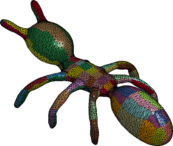
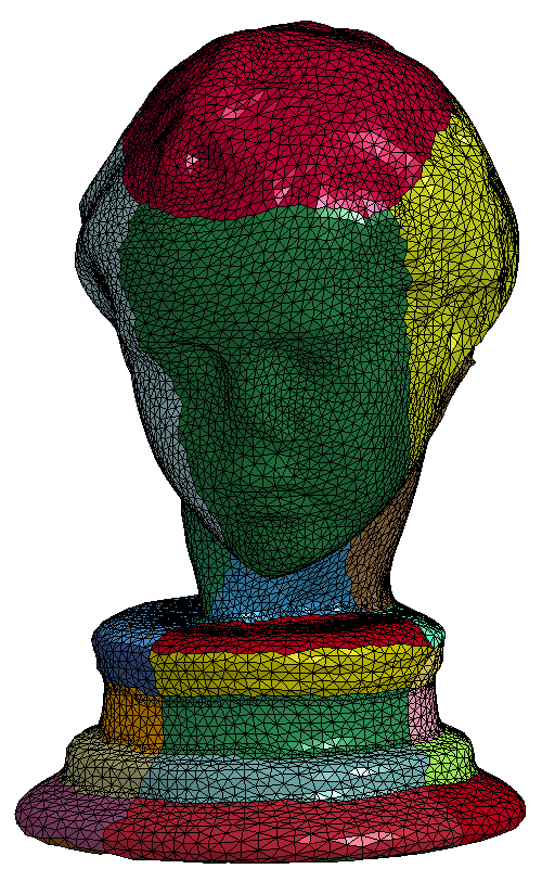
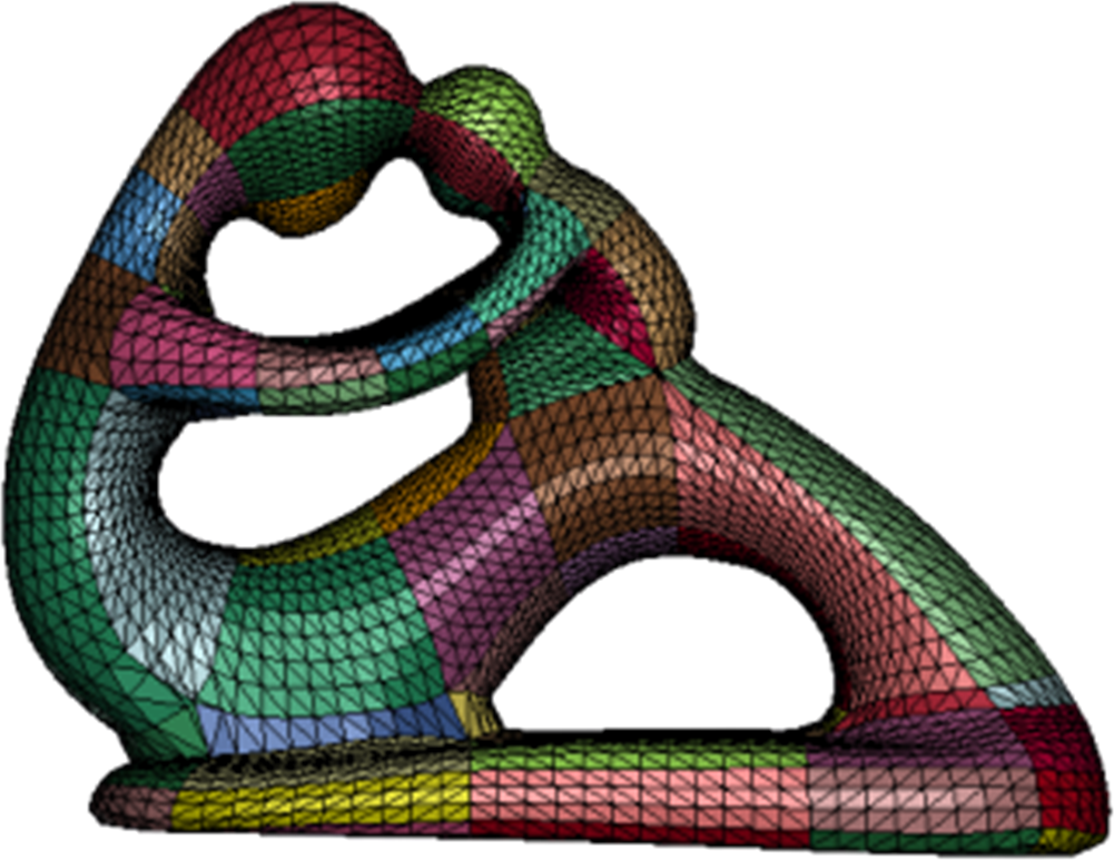
	(a)
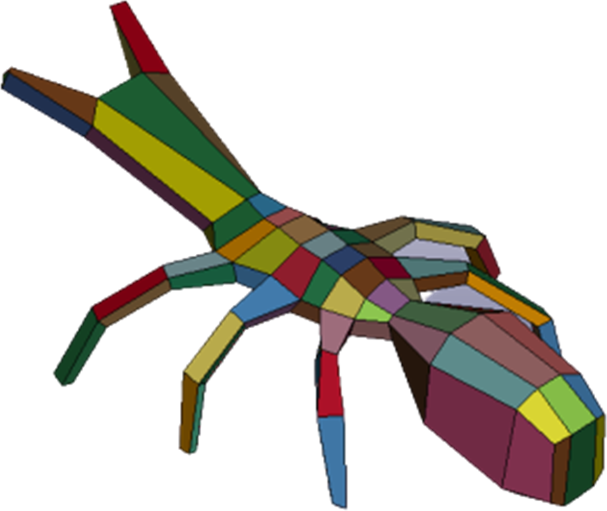
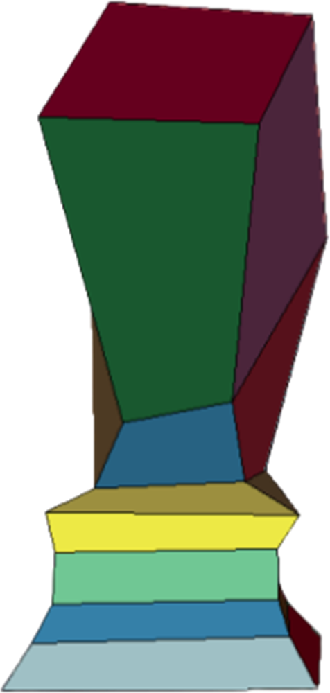
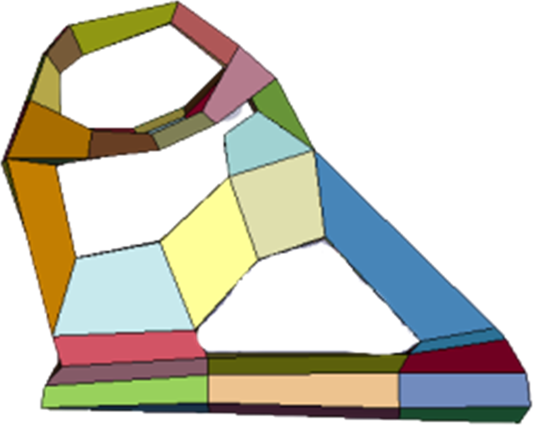
	(b)
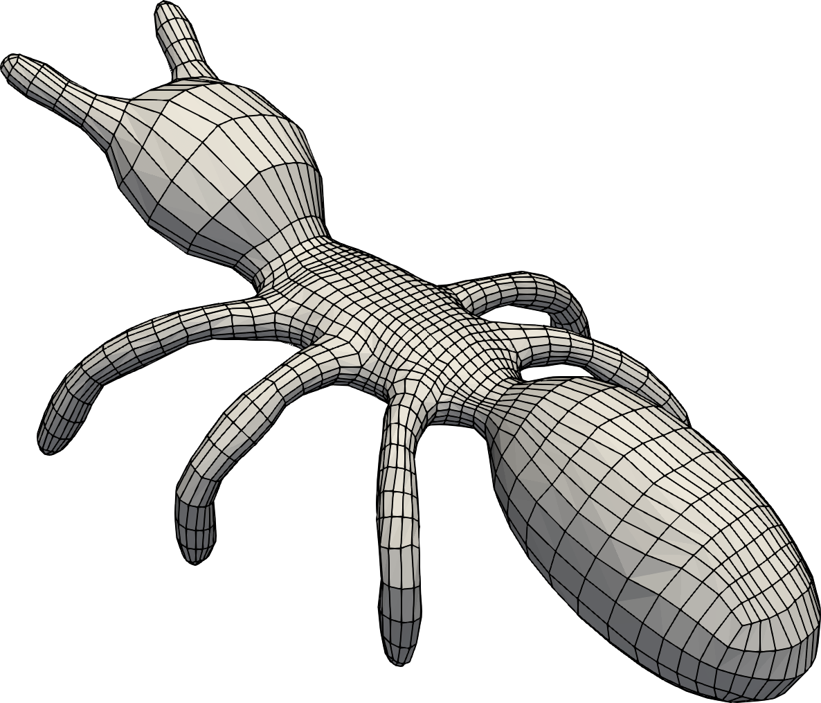
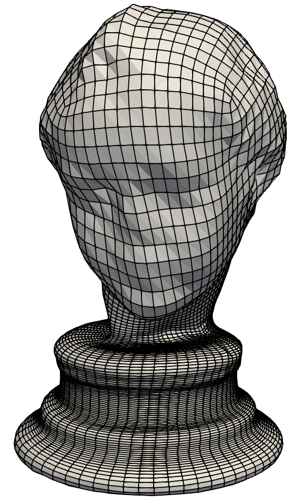
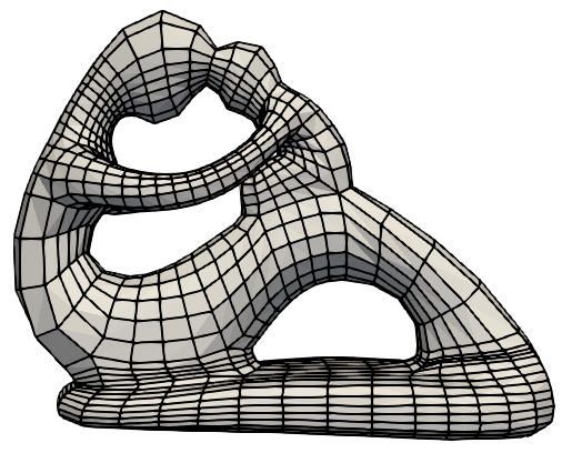
	(c)
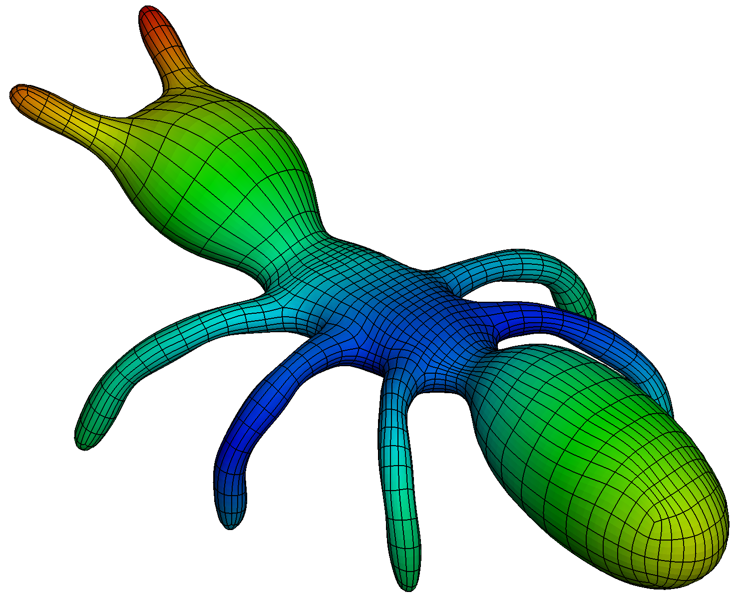
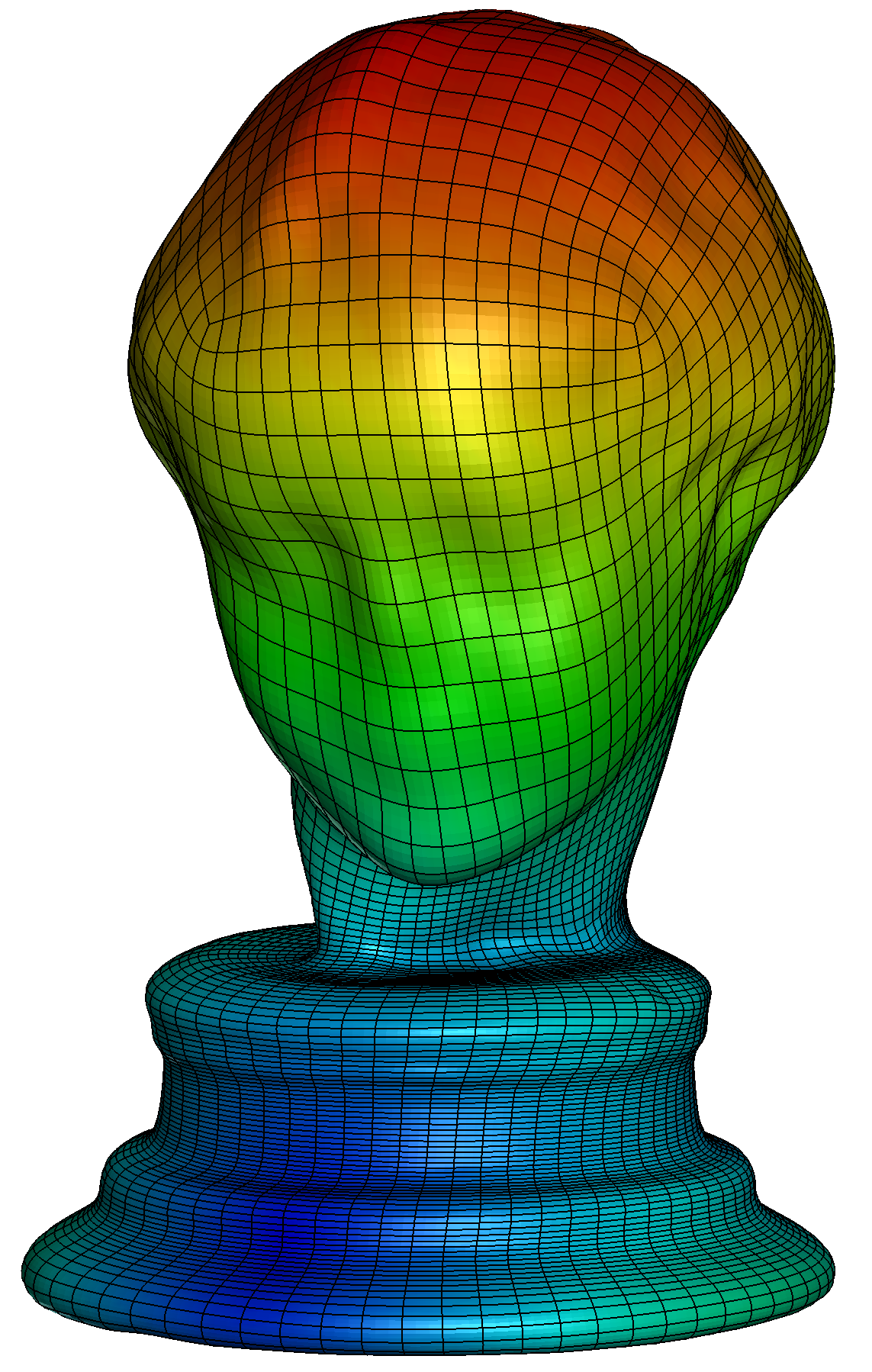
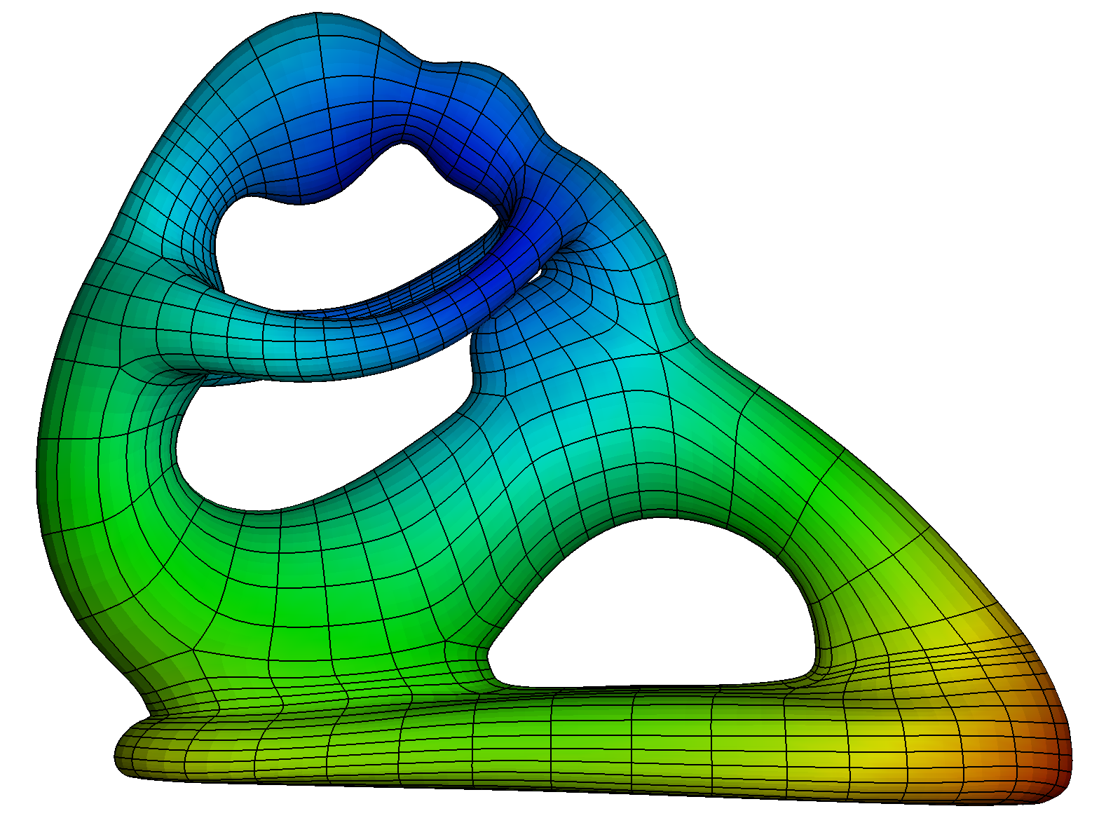
	(d)

Figure 7: Results of ant, bust, and fertility model. (a) Surface triangle meshes and segmentation results; (b) Polycube structures; (c) All-hex control meshes; (d) Volumetric splines with IGA results of eigenvalue analysis in LS-DYNA.

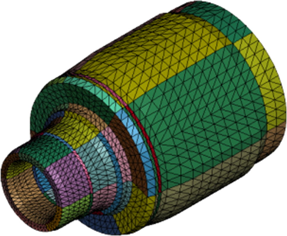
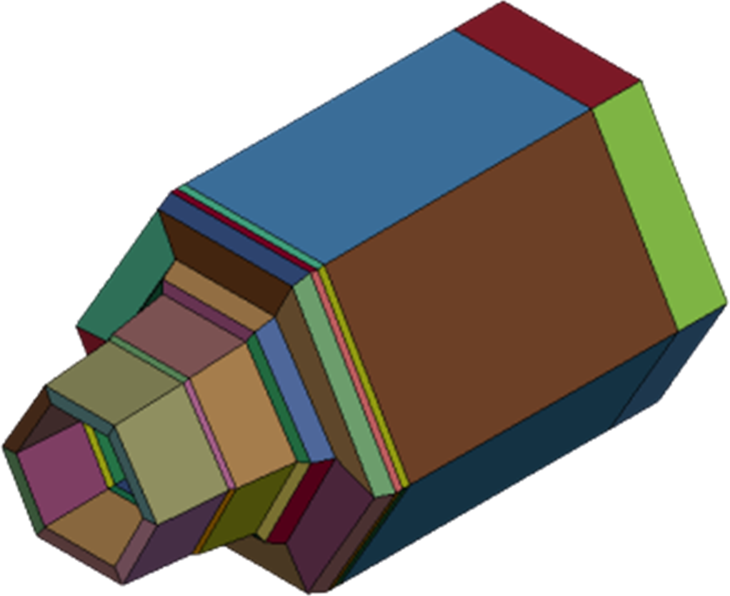
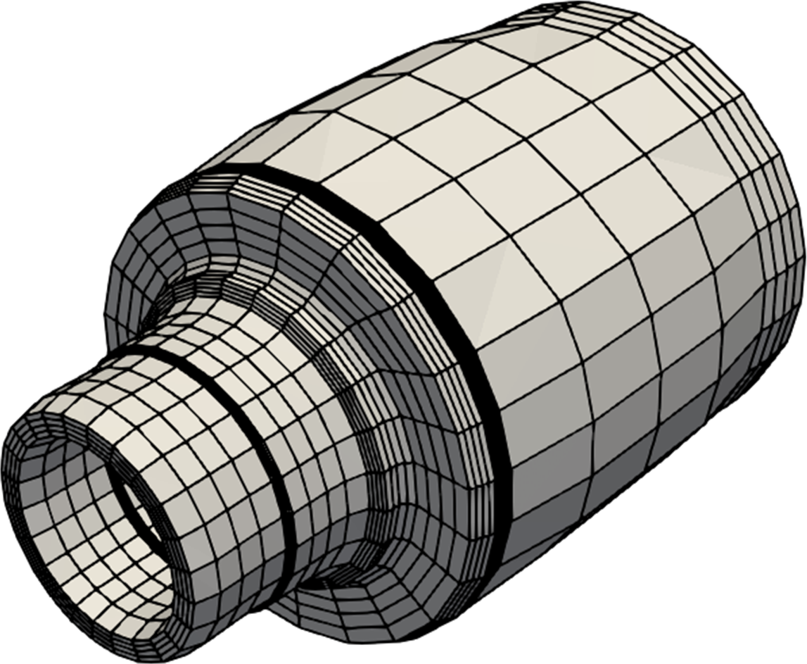
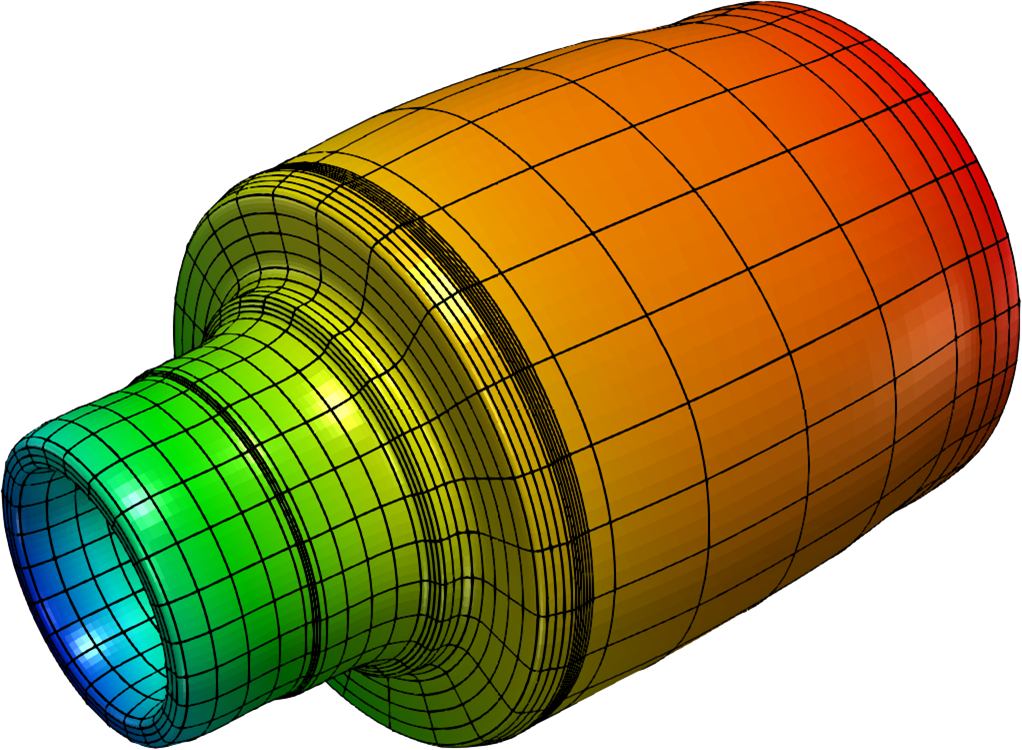
(a)	(b)	(c)	(d)

Figure 8: Results of joint model. (a) Surface triangle meshes and segmentation results; (b) Polycube structures; (c) All-hex control meshes; (d) Volumetric splines with IGA results of solving Poisson equation in LS-DYNA.

6 Conclusion and future work

In this paper, we present two software packages (HexGen and Hex2Spline) for IGA applications in LS-DYNA. The main goal of HexGen and Hex2Spline is to make our pipeline accessible to industrial and academic communities who are interested in real-world engineering applications. The all-hex mesh generation program (HexGen) can generate all-hex meshes. It consists of four executable files, namely segmentation module (Segmentation.exe), polycube construction module (Polycube.exe), all-hex mesh generation module (ParametricMapping.exe) and quality improvement module (Quality.exe). The volumetric spline construction program (Hex2Spline.exe) is developed based on the spline construction method in wei17a . Users can generate a volumetric spline model given any unstructured hex mesh and output a BEXT file to perform IGA in LS-DYNA. Both programs are compiled in executable files and can be easily run in the Command Prompt (cmd) in platform. The rod model is used to explain how to use these two programs in detail. We also tested our software package using several other models.

In conclusion, we integrate our hex mesh generation and volumetric spline construction techniques and develop a software platform to create IGA models for LS-DYNA. Our software also has limitations that we will address in our future work. First, the hex mesh generation module is semi-automatic and needs user intervention to create polycube structure. We will improve the underneath algorithm and make polycube construction more automatic. In addition, our software cannot guarantee to generate good quality hex mesh for complex geometry. Therefore, in the future we will expand our software package to use hex-dominant meshing methods to create hybrid meshes for IGA applications.

Appendix

A1 Input text file to correct segmentation result from Segmentation.exe

In this section, we describe the data format of the input text file used in Segmentation.exe to correct the segmentation result. One can prepare this file to move elements on the wrong patch to the desired patch. In this text file, each row has two values to define this modification of one element (see List 1). The first value indicates the element index in the triangular mesh and the second value is the desired patch index. Segmentation.exe can read this file through option -m to improve the segmentation result.

⬇

1 355 1

2 356 1

3 361 1

4 362 1

5 365 1

6 366 1

7 369 1

8 370 1

9 495 6

10 496 6

11 499 6

12 500 6

List 1: Snippets of the input text file

A2 Further segmentation in LS-PrePost

In this section, we introduce how to perform further segmentation in LS-PrePost and obtain an admissible segmentation for polycube construction. It mainly involves reassigning elements to different patches and there are four steps to achieve this (see Fig. A1): 1) click move/copy tab; 2) select elements; 3) reassign the patch ID; and 4) click the Apply button to finish.

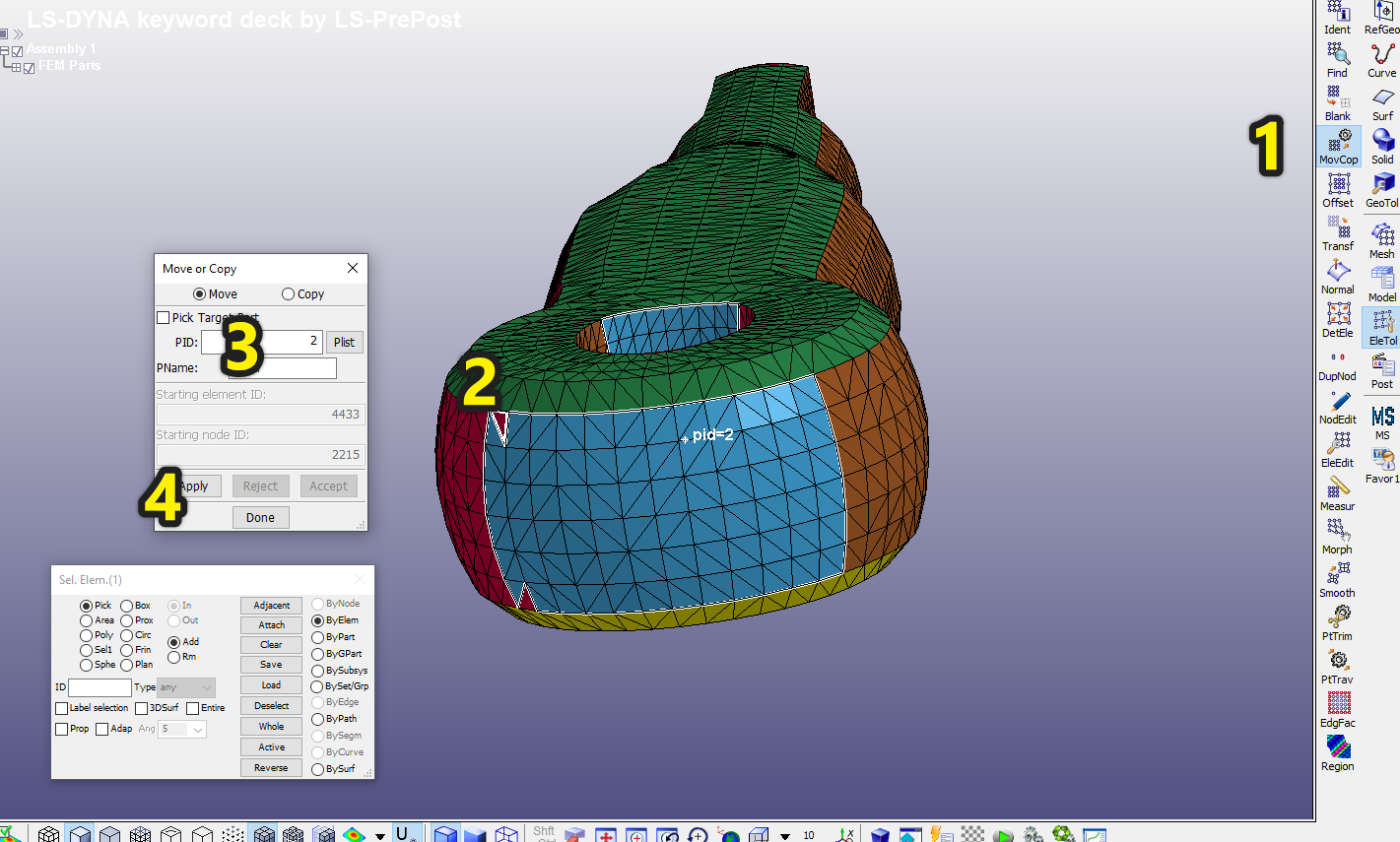
Figure A1: The detailed operations for further segmentation.

A3 Building the interior connectivity of polycube structure in LS-PrePost

In this section, we use the rod model to introduce how to build the interior connectivity of polycube structure in LS-PrePost. There are four steps to create one cubic region ( see Fig. A2): 1) click EleEdt tab; 2) select Elem Type as Hexa; 3) select eight nodes to define cubic regions, you can also check the selection on the float box; and 4) click the Accept button to finish. By repeating the same operation, we generate the polycube structure with multiple cubic regions to split the volumetric domain of the geometry.

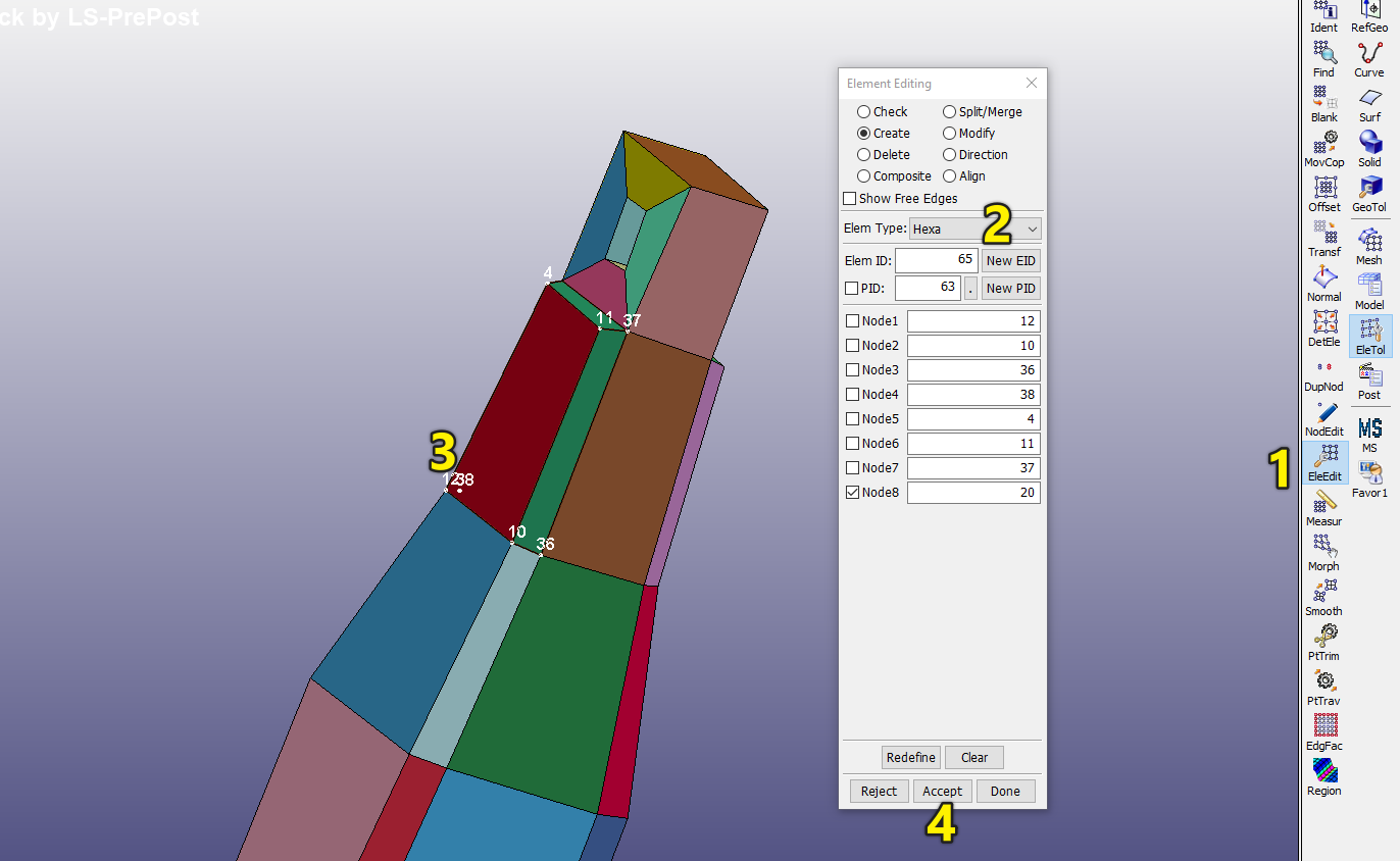
Figure A2: The detailed operations to build the interior connectivity of polycube structure.

A4 Output text file from Polycube.exe

In CLI program (PolyCube.exe), we output a .k file which contains the corners and their connectivity for the boundary surface of the polycube. It can be directly opened by LS-PrePost. If one intends to use other software to build a polycube structure, we also provide option to output the corners, edges, and faces of the polycube in three separate text files (see Lists 2-4). In the corner file, each row depicts the associated vertex ($v_{i}$) information. The first value indicates the index of the vertex in the triangles mesh, the last three values are its x, y, z coordinates ($x_{i},y_{i},z_{i}$). In the edge file, each row uses the indices of two corners to define the edge between them. These indices should agree with the corner file. The face file stores the information of boundary faces on polycube structure. Each row contains four vertex indices in counter-clockwise order to define the connectivity of one face.

⬇

121 4.06622 0.0052 2.31336

2143 16.4588 0.7317 2.29912

3153 4.0543 3.3803 2.31406

4371 16.4604 2.67402 4.12666

5391 13.5206 0.65268 2.07416

List 2: Snippets of the corner file

⬇

171,446

2436,446

3436,442

4371,442

51464,1639

61601,1639

List 3: Snippets of the edge file

⬇

171,446,436,442

21464,1639,1601,1503

31439,1664,1639,1464

41744,1917,1877,1784

51246,1784,1877,153

List 4: Snippets of the face file

A5 Sharp feature file for Quality.exe and Hex2Spline.exe

This section describes how to manually define sharp features for Quality.exe and Hex2Spline.exe. One can prepare an input file including the sharp feature information with the help of Paraview. There are four steps (see Fig. A3): 1) select the points along the sharp feature; 2) use Extract selection function to extract the indices of these nodes; 3) check the selected points information under ”Properties”; and 4) copy the index to ”sharp.txt” file and use it as the input sharp feature file for Quality.exe and Hex2Spline.exe.

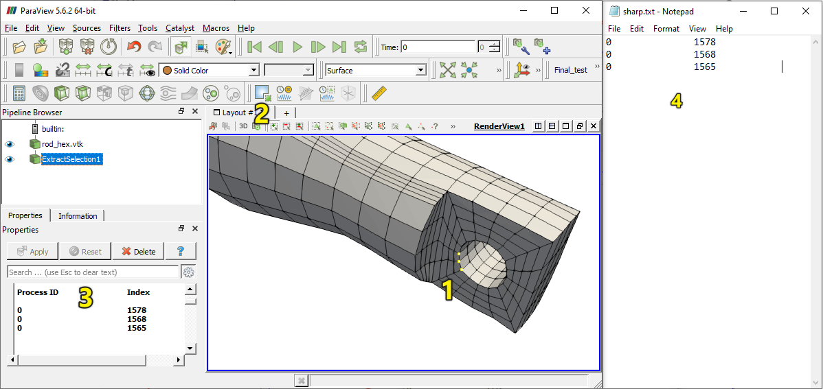
Figure A3: The detailed operations to create user-defined sharp features.

A6 Input BEXT file for LS-DYNA

In this section, we describe the data format of BEXT file for IGA in LS-DYNA. The BEXT file consists of two parts to store the spline information: 1) control point (Fig. A4A); and 2) Bézier element including the indices of control points supported by this Bézier element (Fig. A4B) and the Bézier extraction matrix (Fig. A4C). The Bézier extraction matrix is output row by row and the format of each row depends on the number of non-zero values in this row. If this row has less than 20 non-zeros, a sparse format is used to store their column indices and values; otherwise, a dense format is used to store all values in this row. To distinguish between two formats, a sparse row begins with s while a dense row begins with d.

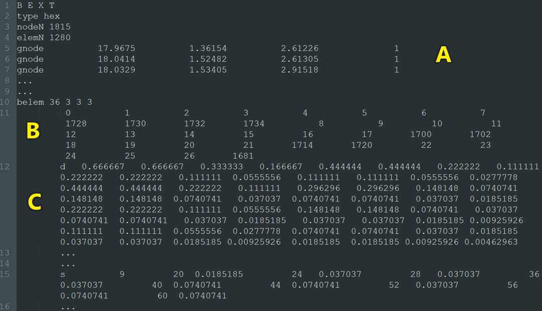
Figure A4: Snippets of the BEXT file.

References

- (1) Ahrens, J., Geveci, B., Law, C.: Paraview: An end-user tool for large data visualization. The Visualization Handbook 717 (2005)
- (2) Bajaj, C., Schaefer, S., Warren, J., Xu, G.: A subdivision scheme for hexahedral meshes. The Visual Computer 18, 343–356 (2002)
- (3) Balay, S., Gropp, W.D., McInnes, L.C., Smith, B.F.: Efficient management of parallelism in object-oriented numerical software libraries. In: Modern Software Tools for Scientific Computing, pp. 163–202. Springer (1997)
- (4) Blacker, T.D., Stephenson, M.B.: Paving: A new approach to automated quadrilateral mesh generation. International Journal for Numerical Methods in Engineering 32(4), 811–847 (1991)
- (5) Burkhart, D., Hamann, B., Umlauf, G.: Iso-geometric finite element analysis based on Catmull-Clark subdivision solids. Computer Graphics Forum 29, 1575–1584 (2010)
- (6) Dalcin, L., Collier, N., Vignal, P., Côrtes, A.M., Calo, V.M.: PetIGA: A framework for high-performance isogeometric analysis. Computer Methods in Applied Mechanics and Engineering 308, 151–181 (2016)
- (7) De Falco, C., Reali, A., Vázquez, R.: GeoPDEs: A research tool for isogeometric analysis of PDEs. Advances in Engineering Software 42(12), 1020–1034 (2011)
- (8) Eck, M., DeRose, T., Duchamp, T., Hoppe, H., Lounsbery, M., Stuetzle, W.: Multiresolution analysis of arbitrary meshes. In: Proceedings of the 22nd Annual Conference on Computer Graphics and Interactive Techniques, pp. 173–182 (1995)
- (9) Floater, M.S.: Parametrization and smooth approximation of surface triangulations. Computer Aided Geometric Design 14(3), 231–250 (1997)
- (10) Folwell, N., Mitchell, S.: Reliable whisker weaving via curve contraction. Engineering with Computers 15(3), 292–302 (1999)
- (11) Forsey, D.R., Bartels, R.H.: Hierarchical B-spline refinement. Computer Graphics 22, 205–212 (1988)
- (12) Giannelli, C., Jüttler, B., Speleers, H.: THB-splines: The truncated basis for hierarchical splines. Computer Aided Geometric Design 29, 485–498 (2012)
- (13) Giannelli, C., Jüttler, B., Speleers, H.: Strongly stable bases for adaptively refined multilevel spline spaces. Advances in Computational Mathematics 40(2), 459–490 (2014)
- (14) Gregson, J., Sheffer, A., Zhang, E.: All-Hex mesh generation via volumetric polycube deformation. Computer Graphics Forum 30(5), 1407–1416 (2011)
- (15) Guennebaud, G., Jacob, B.: Eigen v3 (2010). http://eigen.tuxfamily.org
- (16) He, Y., Wang, H., Fu, C., Qin, H.: A divide-and-conquer approach for automatic polycube map construction. Computers & Graphics 33(3), 369–380 (2009)
- (17) Hu, K., Zhang, Y.J.: Centroidal Voronoi tessellation based polycube construction for adaptive all-hexahedral mesh generation. Computer Methods in Applied Mechanics and Engineering 305, 405–421 (2016)
- (18) Hughes, T.J.R., Cottrell, J.A., Bazilevs, Y.: Isogeometric analysis: CAD, finite elements, NURBS, exact geometry, and mesh refinement. Computer Methods in Applied Mechanics and Engineering 194, 4135–4195 (2005)
- (19) Intel: Math kernel library. https://software.intel.com/en-us/intel-mkl
- (20) Lai, Y., Liu, L., Zhang, Y., Chen, J., Fang, E., Lua, J.: Rhino 3D to Abaqus design-through-analysis: A T-spline based IGA software platform. In: Y. Bazilevs, K. Takizawa (eds.) The Edited Volume of the Modeling and Simulation in Science, Engineering and Technology Book Series Devoted to AFSI 2014 - A Birthday Celebration Conference for Tayfun Tezduyar. Springer (2015)
- (21) Lai, Y., Zhang, Y.J., Liu, L., Wei, X., Fang, E., Lua, J.: Integrating CAD with Abaqus: A practical isogeometric analysis software platform for industrial applications. Computers and Mathematics with Applications 74(7), 1648–1660 (2017)
- (22) Lin, J., Jin, X., Fan, Z., Wang, C.: Automatic polycube-maps. In: Advances in Geometric Modeling and Processing, Lecture Notes in Computer Science, vol. 4975, pp. 3–16. Springer Berlin / Heidelberg (2008)
- (23) Liu, L., Zhang, Y., Hughes, T.J., Scott, M.A., Sederberg, T.W.: Volumetric T-spline construction using Boolean operations. Engineering with Computers 30(4), 425–439 (2014)
- (24) Liu, L., Zhang, Y., Liu, Y., Wang, W.: Feature-preserving T-mesh construction using skeleton-based polycubes. Computer Aided Design 58, 162–172 (2015)
- (25) Livermore Software Technology Corporation: LS-DYNA Keyword User’s Manual (2007)
- (26) Nieser, M., Reitebuch, U., Polthier, K.: Cubecover- parameterization of 3d volumes. Computer Graphics Forum 30(5), 1397–1406 (2011)
- (27) Pauletti, M.S., Martinelli, M., Cavallini, N., Antolin, P.: Igatools: An isogeometric analysis library. SIAM Journal on Scientific Computing 37(4), C465—-C496 (2015)
- (28) Price, M.A., Armstrong, C.G.: Hexahedral mesh generation by medial surface subdivision: Part II. Solids with flat and concave edges. International Journal for Numerical Methods in Engineering 40(1), 111–136 (1997)
- (29) Price, M.A., Armstrong, C.G., Sabin, M.A.: Hexahedral mesh generation by medial surface subdivision: Part I. Solids with convex edges. International Journal for Numerical Methods in Engineering 38(19), 3335–3359 (1995)
- (30) Qian, J., Zhang, Y.: Automatic unstructured all-hexahedral mesh generation from B-Reps for non-manifold CAD assemblies. Engineering with Computers 28(4), 345–359 (2012)
- (31) Qian, J., Zhang, Y., Wang, W., Lewis, A.C., Qidwai, M.A.S., Geltmacher, A.B.: Quality improvement of non-manifold hexahedral meshes for critical feature determination of microstructure materials. International Journal for Numerical Methods in Engineering 82(11), 1406–1423 (2010)
- (32) Schneiders, R.: A grid-based algorithm for the generation of hexahedral element meshes. Engineering with computers 12(3-4), 168–177 (1996)
- (33) Schneiders, R.: An algorithm for the generation of hexahedral element meshes based on an octree technique. 6th International Meshing Roundtable pp. 195–196 (1997)
- (34) Sederberg, T.W., Cardon, D.L., Finnigan, G.T., North, N.S., Zheng, J., Lyche, T.: T-spline Simplification and Local Refinement. In: ACM SIGGRAPH, pp. 276–283 (2004)
- (35) Sederberg, T.W., Zheng, J., Bakenov, A., Nasri, A.: T-splines and T-NURCCs. ACM Transactions on Graphics 22, 477–484 (2003)
- (36) Staten, M., Kerr, R., Owen, S., Blacker, T.: Unconstrained paving and plastering: Progress update. Proceedings of 15th International Meshing Roundtable pp. 469–486 (2006)
- (37) Tarini, M., Hormann, K., Cignoni, P., Montani, C.: polycube-maps. ACM Transactions on Graphics 23(3), 853–860 (2004)
- (38) Vuong, A.V., Giannelli, C., Jüttler, B., Simeon, B.: A hierarchical approach to adaptive local refinement in isogeometric analysis. Computer Methods in Applied Mechanics and Engineering 200, 3554–3567 (2011)
- (39) Wang, W., Zhang, Y., Liu, L., Hughes, T.J.R.: Trivariate solid T-spline construction from boundary triangulations with arbitrary genus topology. Computer Aided Design 45(2), 351–360 (2013)
- (40) Wang, W., Zhang, Y., Xu, G., Hughes, T.J.R.: Converting an unstructured quadrilateral/hexahedral mesh to a rational T-spline. Computational Mechanics 50(1), 65–84 (2012)
- (41) Wei, X., Zhang, Y., Hughes, T.J.R.: Truncated hierarchical tricubic C0 spline construction on unstructured hexahedral meshes for isogeometric analysis applications. Computers and Mathematics with Applications 74(9), 2203–2220 (2017)
- (42) Zhang, Y.: Geometric Modeling and Mesh Generation from Scanned Images. Chapman and Hall/CRC (2016)
- (43) Zhang, Y., Bajaj, C.L., Xu, G.: Surface smoothing and quality improvement of quadrilateral/hexahedral meshes with geometric flow. Communications in Numerical Methods in Engineering 25(1), 1–18 (2009)
- (44) Zhang, Y., Wang, W., Hughes, T.J.R.: Solid T-spline construction from boundary representations for genus-zero geometry. Computer Methods in Applied Mechanics and Engineering 249, 185–197 (2012)