Approximate Midpoint Policy Iteration for Linear Quadratic Control

Abstract

We present a midpoint policy iteration algorithm to solve linear quadratic optimal control problems in both model-based and model-free settings. The algorithm is a variation of Newton’s method, and we show that in the model-based setting it achieves cubic convergence, which is superior to standard policy iteration and policy gradient algorithms that achieve quadratic and linear convergence, respectively. We also demonstrate that the algorithm can be approximately implemented without knowledge of the dynamics model by using least-squares estimates of the state-action value function from trajectory data, from which policy improvements can be obtained. With sufficient trajectory data, the policy iterates converge cubically to approximately optimal policies, and this occurs with the same available sample budget as the approximate standard policy iteration. Numerical experiments demonstrate effectiveness of the proposed algorithms.

1 Introduction

With the recent confluence of reinforcement learning and data-driven optimal control, there is renewed interest in fully understanding convergence, sample complexity, and robustness in both “model-based” and “model-free” algorithms. Linear quadratic problems in continuous spaces provide benchmarks where strong theoretical statements can be made. In practice, it is often difficult or impossible to develop a model of a system from first-principles. In this case, one may use so-called “model-based” system identification methods which attempt to estimate a model of the dynamics from observed sample data, then solve the Riccati equation using the identified system matrices. An approximately optimal control policy is then computed assuming certainty-equivalence [Mania et al.(2019)Mania, Tu, and Recht, Oymak and Ozay(2019), Coppens and Patrinos(2020)] or using robust control approaches to explicitly account for model uncertainty [Dean et al.(2018)Dean, Mania, Matni, Recht, and Tu, Dean et al.(2019)Dean, Mania, Matni, Recht, and Tu, Gravell and Summers(2020), Coppens et al.(2020)Coppens, Schuurmans, and Patrinos]. The analyses in these recent works has focused on providing finite-sample performance/suboptimality guarantees.

As an alternative, so-called “model-free” methods may also be used, which do not attempt to learn a model of the dynamics. The category of policy optimization methods which directly attempt to optimize the control policy, including policy gradient, has received significant attention recently for standard LQR [Fazel et al.(2018)Fazel, Ge, Kakade, and Mesbahi, Bu et al.(2020)Bu, Mesbahi, and Mesbahi], multiplicative-noise LQR [Gravell et al.(2021a)Gravell, Esfahani, and Summers], Markov jump LQR [Jansch-Porto et al.(2020)Jansch-Porto, Hu, and Dullerud], and LQ games related to $\mathcal{H}_{\infty}$ robust control [Zhang et al.(2019)Zhang, Yang, and Basar, Bu et al.(2019)Bu, Ratliff, and Mesbahi].

Between the fully model-based system identification approaches and the fully model-free policy optimization approaches lies another category of methods, which we denote as value function approximation methods. These methods attempt to estimate value functions then compute policies which are optimal with respect to these value functions. This class of methods includes approximate dynamic programming, exemplified by approximate value iteration, which estimates state-value functions, and approximate policy iteration, which estimates state-action value functions. In particular, for LQR problems, approximate policy iteration was studied by [Bradtke et al.(1994)Bradtke, Ydstie, and Barto, Krauth et al.(2019)Krauth, Tu, and Recht] and by [Fazel et al.(2018)Fazel, Ge, Kakade, and Mesbahi, Bu et al.(2020)Bu, Mesbahi, and Mesbahi] under the guise of a quasi-Newton method. For LQ games, approximate policy iteration was studied by [Al-Tamimi et al.(2007)Al-Tamimi, Lewis, and Abu-Khalaf] under the guise of Q-learning, and by [Luo et al.(2020)Luo, Yang, and Liu, Gravell et al.(2021b)Gravell, Ganapathy, and Summers]. Note that approximate policy iteration is sometimes called quasi-Newton or Q-learning.

In stochastic optimal control, the functional Bellman equation gives a sufficient and necessary condition for optimality of a control policy ([Bellman(1959)]). It has been long-known, but perhaps underappreciated, that application of Newton’s method to find the root of the functional Bellman equation in stochastic optimal control is equivalent to the dynamic programming algorithm of policy iteration ([Puterman and Brumelle(1979), Madani(2002)]). In this most general setting, conditions for and rates of convergence are available ([Puterman and Brumelle(1979), Madani(2002)]), but may be difficult or impossible to verify in practice. Furthermore, even representing the value functions and policies and executing the policy iteration updates may be intractable. This motivates the basic approximation of such problems by linear dynamics and quadratic costs over finite-dimensional, infinite-cardinality state and action spaces. In linear-quadratic problems, the Bellman equation becomes a matrix algebraic Riccati equation, and application of the Newton method to the Riccati equation yields the well-known Kleinman-Hewer algorithm. The Newton method has many variations devised to improve the convergence rate and information efficiency, including higher-order methods (such as Halley ([Cuyt and Rall(1985)]), super-Halley ([Gutiérrez and Hernández(2001)]), and Chebyshev ([Argyros and Chen(1993)])), and multi-point methods ([Traub(1964)]), which compute derivatives at multiple points and of which the midpoint method is the simplest member. Some of these have been applied to solving Riccati equations by [Anderson(1978), Guo and Laub(2000), Damm and Hinrichsen(2001), Freiling and Hochhaus(2004), Hernández-Verón and Romero(2018)], but without consideration of the situation when the dynamics are not perfectly known. Our main contributions are:

1. We present a midpoint policy iteration algorithm to solve linear quadratic optimal control problems when the dynamics are both known (Algorithm 1) and unknown (Algorithm 4).

2. We demonstrate that the method converges, and does so at a faster cubic rate than standard policy iteration or policy gradient, which converge at quadratic and linear rates, respectively.

3. We show that approximate midpoint policy iteration converges faster in the model-free setting even with the same available sample budget as the approximate standard policy iteration.

4. We present numerical experiments that illustrate and demonstrate the effectiveness of the algorithms and provide an open-source implementation to facilitate their wider use.

2 Preliminaries

Symbol	Meaning
$\mathbb{R}^{n\times m}$	Space of real-valued $n\times m$ matrices
$\mathbb{S}^{n}$	Space of symmetric real-valued $n\times n$ matrices
$\mathbb{S}^{n}_{+}$	Space of symmetric real-valued positive semidefinite $n\times n$ matrices
$\mathbb{S}^{n}_{++}$	Space of symmetric real-valued strictly positive definite $n\times n$ matrices
$\rho(M)$	Spectral radius (greatest magnitude of an eigenvalue) of a square matrix $M$
$\lVert M\rVert$	Spectral norm (greatest singular value) of a matrix $M$
$\lVert M\rVert_{F}$	Frobenius norm (Euclidean norm of the vector of singular values) of a matrix $M$
$M\otimes N$	Kronecker product of matrices $M$ and $N$
$\operatorname{vec}(M)$	Vectorization of matrix $M$ by stacking its columns
$\operatorname{mat}(v)$	Matricization of vector $v$ such that $\operatorname{mat}(\operatorname{vec}(M))=M$
$\operatorname{svec}(M)$	Symmetric vectorization of matrix $M$ by stacking columns of the upper triangular part, including the main diagonal, with off-diagonal entries multiplied by $\sqrt{2}$ such that $\lVert M\rVert_{F}^{2}=\operatorname{svec}(M)^{\intercal}\operatorname{svec}(M)$
$\operatorname{smat}(v)$	Symmetric matricization of vector $v$ i.e. inverse operation of $\operatorname{svec}(\cdot)$ such that $\operatorname{smat}(\operatorname{svec}(M))=M$
$M\succ(\succeq)\ 0$	Matrix $M$ is positive (semi)definite
$M\succ(\succeq)\ N$	Matrix $M$ succeeds matrix $N$ as $M-N\succ(\succeq)\ 0$

The infinite-horizon average-cost time-invariant linear quadratic regulator (LQR) problem is

$$\underset{{\pi\in\Pi}}{\text{minimize}}\quad \lim_{T\to\infty}\frac{1}{T}\mathbb{E}_{x_{0},w_{t}}\sum_{t=0}^{T}\begin{bmatrix}x_{t}\\ u_{t}\end{bmatrix}^{\intercal}\begin{bmatrix}Q_{xx}&Q_{xu}\\ Q_{ux}&Q_{uu}\end{bmatrix}\begin{bmatrix}x_{t}\\ u_{t}\end{bmatrix},$$ (1)

subject to $$x_{t+1}=Ax_{t}+Bu_{t}+w_{t},$$

where $x_{t}\in\mathbb{R}^{n}$ is the system state, $u_{t}\in\mathbb{R}^{m}$ is the control input, and $w_{t}$ is i.i.d. process noise with zero mean and covariance matrix $W$. The state-to-state system matrix $A\in\mathbb{R}^{n\times n}$ and input-to-state system matrix $B\in\mathbb{R}^{n\times m}$ may or may not be known; we present algorithms for both settings. The optimization is over the space $\Pi$ of (measurable) history dependent feedback policies $\pi=\{\pi_{t}\}_{t=0}^{\infty}$ with $u_{t}=\pi_{t}(x_{0:t},u_{0:t-1})$. The penalty weight matrix

$$Q=\begin{bmatrix}Q_{xx}&Q_{xu}\\ Q_{ux}&Q_{uu}\end{bmatrix}\in\mathbb{S}^{n+m}$$

has blocks $Q_{xx}$, $Q_{uu}$, $Q_{xu}=Q_{ux}^{\intercal}$ which quadratically penalize deviations of the state, input, and product of state and input from the origin, respectively. We assume the pair $(A,B)$ is stabilizable, the pair $(A,Q_{xx}^{1/2})$ is detectable, and the penalty matrices satisfy the definiteness condition $Q\succ 0$, in order to ensure feasibility of the problem (see [Anderson and Moore(2007)]). An LQR problem is fully described by the tuple of problem data $(A,B,Q)$, which are fixed after problem definition. In general, operators denoted by uppercase calligraphic letters depend on the problem data $(A,B,Q)$, but we will not explicitly notate this for brevity; dependence on other parameters will be denoted explicitly by functional arguments. We index over time in the evolution of a dynamical system with the letter $t$, and index over iterations of an algorithm with the letter $k$.

Dynamic programming can be used to show that the optimal policy that solves (1) is linear state-feedback

$$u_{t}=Kx_{t},$$

where the gain matrix $K=\mathcal{K}(P)$ is expressed through the linear-fractional operator $\mathcal{K}$

$$\mathcal{K}(P) \coloneqq-\left(Q_{uu}+B^{\intercal}PB\right)^{-1}(Q_{ux}+B^{\intercal}PA),$$

and $P$ is the optimal value matrix found by solving the algebraic Riccati equation (ARE)

$$\mathcal{R}(P)=0,$$ (2)

where $\mathcal{R}$ is the quadratic-fractional Riccati operator

$$\mathcal{R}(P) \coloneqq-P+Q_{xx}+A^{\intercal}PA-(Q_{xu}+A^{\intercal}PB)\left(Q_{uu}+B^{\intercal}PB\right)^{-1}(Q_{ux}+B^{\intercal}PA).$$

The optimal gain and value matrix operators can be expressed more compactly as

$$\mathcal{K}(P) =-\mathcal{H}_{uu}^{-1}(P)\mathcal{H}_{ux}(P),$$

$$\mathcal{R}(P) =-P+\mathcal{H}_{xx}(P)-\mathcal{H}_{xu}(P)\mathcal{H}_{uu}^{-1}(P)\mathcal{H}_{ux}(P)$$

where $\mathcal{H}$ is the state-action value matrix operator

$$\mathcal{H}(P)=\begin{bmatrix}\mathcal{H}_{xx}(P)&\mathcal{H}_{xu}(P)\\ \mathcal{H}_{ux}(P)&\mathcal{H}_{uu}(P)\end{bmatrix}\coloneqq Q+\begin{bmatrix}A&B\end{bmatrix}^{\intercal}P\begin{bmatrix}A&B\end{bmatrix}.$$

The discrete-time Lyapunov equation with matrix $F$ and symmetric matrix $S$ is

$$X=F^{\intercal}XF+S,$$

whose solution we denote by $X=\texttt{DLYAP}(F,S)$, which is unique if $F$ is Schur stable.

2.1 Derivatives of the Riccati operator

The first total derivative of the Riccati operator evaluated at point $P\in\mathbb{S}^{n}$ is denoted as $\mathcal{R}^{\prime}(P)\in\mathbb{S}^{n}\times\mathbb{S}^{n}$. With a slight abuse of notation, the first directional derivative of the Riccati operator evaluated at point $P$ in direction $X$ is denoted as $\mathcal{R}^{\prime}(P,X)\in\mathbb{S}^{n}$. Computation of the first directional derivative is straightforward and follows e.g. the derivation given by [Luo et al.(2020)Luo, Yang, and Liu]. The general limit definition of this derivative is

$$\mathcal{R}^{\prime}(P,X)\coloneqq\lim_{\varepsilon\to 0}\frac{\mathcal{R}(P+\varepsilon X)-\mathcal{R}(P)}{\varepsilon}=\left.\frac{d\mathcal{R}(P+\varepsilon X)}{d\varepsilon}\right|_{\varepsilon=0}$$

Notice that since $\mathcal{R}:\mathbb{S}^{n}\to\mathbb{S}^{n}$ it follows that $\mathcal{R}^{\prime}(\cdot,\cdot):\mathbb{S}^{n}\times\mathbb{S}^{n}\to\mathbb{S}^{n}$. In evaluating the first directional derivative, it will be useful note that

$$\mathcal{H}(P+\varepsilon X)=Q+\begin{bmatrix}A&B\end{bmatrix}^{\intercal}(P+\varepsilon X)\begin{bmatrix}A&B\end{bmatrix}.$$

The first derivative is then

$$\mathcal{R}^{\prime}(P,X) =\left.\frac{d\mathcal{R}(P+\varepsilon X)}{d\varepsilon}\right|_{\varepsilon=0}$$

$$=\left.\frac{d}{d\varepsilon}\left[-(P+\varepsilon X)+\mathcal{H}_{xx}(P+\varepsilon X)-\mathcal{H}_{xu}(P+\varepsilon X)\mathcal{H}_{uu}^{-1}(P+\varepsilon X)\mathcal{H}_{ux}(P+\varepsilon X)\right]\right|_{\varepsilon=0}$$

At this point it will be useful to evaluate the following expressions:

$$\left.\frac{d\mathcal{H}(P+\varepsilon X)}{d\varepsilon}\right|_{\varepsilon=0} =\left.\frac{d}{d\varepsilon}\left[Q+\begin{bmatrix}A&B\end{bmatrix}^{\intercal}(P+\varepsilon X)\begin{bmatrix}A&B\end{bmatrix}\right]\right|_{\varepsilon=0}$$

$$=\begin{bmatrix}A&B\end{bmatrix}^{\intercal}X\begin{bmatrix}A&B\end{bmatrix},$$

and

$$\left.\frac{d\mathcal{H}_{uu}^{-1}(P+\varepsilon X)}{d\varepsilon}\right|_{\varepsilon=0} =-\mathcal{H}_{uu}^{-1}(P)\left.\frac{d\mathcal{H}_{uu}(P+\varepsilon X)}{d\varepsilon}\right|_{\varepsilon=0}\mathcal{H}_{uu}^{-1}(P)$$

$$=-\left(Q_{uu}+B^{\intercal}PB\right)^{-1}\left(B^{\intercal}XB\right)\left(Q_{uu}+B^{\intercal}PB\right)^{-1},$$

where we used the rule for a derivative of a matrix inverse e.g. as in [Selby(1974)]. Continuing with the first derivative,

$$\mathcal{R}^{\prime}(P,X) =\left.\frac{d}{d\varepsilon}\left[-(P+\varepsilon X)+\mathcal{H}_{xx}(P+\varepsilon X)-\mathcal{H}_{xu}(P+\varepsilon X)\mathcal{H}_{uu}^{-1}(P+\varepsilon X)\mathcal{H}_{ux}(P+\varepsilon X)\right]\right|_{\varepsilon=0}$$

$$=-\left.\frac{d}{d\varepsilon}\left[P+\varepsilon X\right]\right|_{\varepsilon=0}+\left.\frac{d}{d\varepsilon}\left[\mathcal{H}_{xx}(P+\varepsilon X)\right]\right|_{\varepsilon=0}$$

$$\quad-\left.\frac{d}{d\varepsilon}\left[\mathcal{H}_{xu}(P+\varepsilon X)\right]\right|_{\varepsilon=0}\mathcal{H}_{uu}^{-1}(P)\mathcal{H}_{ux}(P)$$

$$\quad-\mathcal{H}_{xu}(P)\left.\frac{d}{d\varepsilon}\left[\mathcal{H}_{uu}^{-1}(P+\varepsilon X)\right]\right|_{\varepsilon=0}\mathcal{H}_{ux}(P)$$

$$\quad-\mathcal{H}_{xu}(P)\mathcal{H}_{uu}^{-1}(P)\left.\frac{d}{d\varepsilon}\left[\mathcal{H}_{ux}(P+\varepsilon X)\right]\right|_{\varepsilon=0}$$

$$=-X+A^{\intercal}XA$$

$$\quad-A^{\intercal}XB\left(Q_{uu}+B^{\intercal}PB\right)^{-1}(Q_{ux}+B^{\intercal}PA)$$

$$\quad-(Q_{xu}+A^{\intercal}PB)\left(Q_{uu}+B^{\intercal}PB\right)^{-1}B^{\intercal}XA$$

$$\quad+A^{\intercal}PB\left(Q_{uu}+B^{\intercal}PB\right)^{-1}B^{\intercal}XB\left(Q_{uu}+B^{\intercal}PB\right)^{-1}B^{\intercal}PA$$ (3)

where we used the product rule for matrix derivatives.

2.2 Identities

Considering two symmetric matrices $P,X$ and the related gains

$$K =\mathcal{K}(P)=-\left(Q_{uu}+B^{\intercal}PB\right)^{-1}(Q_{ux}+B^{\intercal}PA),$$

$$L =\mathcal{K}(X)=-\left(Q_{uu}+B^{\intercal}XB\right)^{-1}(Q_{ux}+B^{\intercal}XA),$$

we have

$$Q_{ux}+Q_{uu}K =-B^{\intercal}P(A+BK),$$

$$K^{\intercal}Q_{ux}+K^{\intercal}Q_{uu}K =-(BK)^{\intercal}P(A+BK).$$

Thus the Riccati operator $\mathcal{R}(P)$ can be rewritten as

$$\mathcal{R}(P) =-P+Q_{xx}+Q_{xu}K+A^{\intercal}P(A+BK)$$

$$=-P+Q_{xx}+Q_{xu}K-(BK)^{\intercal}P(A+BK)+(A+BK)^{\intercal}P(A+BK)$$

$$=-P+\begin{bmatrix}I\\ K\end{bmatrix}^{\intercal}\begin{bmatrix}Q_{xx}&Q_{xu}\\ Q_{ux}&Q_{uu}\end{bmatrix}\begin{bmatrix}I\\ K\end{bmatrix}+(A+BK)^{\intercal}P(A+BK)$$

$$=-P+\begin{bmatrix}I\\ K\end{bmatrix}^{\intercal}\left(Q+\begin{bmatrix}A&B\end{bmatrix}^{\intercal}P\begin{bmatrix}A&B\end{bmatrix}\right)\begin{bmatrix}I\\ K\end{bmatrix},$$

and the derivative $\mathcal{R}^{\prime}(X,P)$ can be written using (3) as

$$\mathcal{R}^{\prime}(X,P) =-P+(A+BL)^{\intercal}P(A+BL).$$

and we have the identity

$$\mathcal{R}(P)-\mathcal{R}^{\prime}(X,P) =\begin{bmatrix}I\\ K\end{bmatrix}^{\intercal}Q\begin{bmatrix}I\\ K\end{bmatrix}+(A+BK)^{\intercal}P(A+BK)-(A+BL)^{\intercal}P(A+BL).$$ (4)

In the case of $X=P$, identity (4) specializes to

$$\mathcal{R}(P)-\mathcal{R}^{\prime}(P,P) =\begin{bmatrix}I\\ K\end{bmatrix}^{\intercal}Q\begin{bmatrix}I\\ K\end{bmatrix}.$$ (5)

3 Generic Newton methods

First we consider finding a solution to the equation $f(x)=0$ where $f:\mathbb{R}^{n}\to\mathbb{R}^{n}$, whose total derivative at a point $x$ is $f^{\prime}(x)\in\mathbb{R}^{n\times n}$. The methods under consideration can be understood and derived as the numerical integration of the following Newton-Leibniz integral from the second fundamental theorem of calculus:

$$0=f(x)=f\left(x_{k}\right)+\int_{x_{k}}^{x}f^{\prime}(t)dt.$$ (6)

3.1 Newton method

The Newton method, due originally in heavily modified form to [Newton(1711), Raphson(1702)] and originally in the general differential form to [Simpson(1740)] (see the historical notes of [Kollerstrom(1992), Deuflhard(2012)]), begins with an initial guess $x_{0}$ then proceeds with iterations

$$x_{k+1} =x_{k}-f^{\prime}(x_{k})^{-1}f(x_{k}),$$

until convergence. Intuitively, the Newton method forms a linear approximation $f(x_{k})+f^{\prime}(x_{k})(x-x_{k})$ to the function $f$ at $x_{k}$, and assigns the point where the linear approximation crosses $0$ as the next iterate. The Newton method can be derived from (6) by using left rectangular integration.

The Newton update can be rearranged into the Newton equation

$$f^{\prime}(x_{k})(x_{k+1}-x_{k})=-f(x_{k}),$$

where the left-hand side is recognized as the directional derivative of $f$ evaluated at point $x_{k}$ in direction $x_{k+1}-x_{k}$. This rearrangement implies that the Newton method does not require explicit evaluation of the entire total derivative $f^{\prime}(x_{k})$ so long as a suitable direction $x_{k+1}-x_{k}$ can be found which solves the Newton equation. This will become important in the LQR setting as we use this fact to avoid notating and computing large order-4 tensors.

This technique uses derivative information at a single point and is known to achieve quadratic convergence in a neighborhood of the root ([Kantorovich(1948)]). In the setting of both continuous- and discrete-time LQR, this algorithm is known to achieve quadratic convergence globally, as shown by [Kleinman(1968), Hewer(1971), Bu et al.(2020)Bu, Mesbahi, and Mesbahi].

3.2 Mid-point Newton method

The midpoint Newton method, due originally to [Traub(1964)], begins with an initial guess $x_{0}$ then proceeds with iterations

$$x^{N}_{k+1} =x_{k}-f^{\prime}(x_{k})^{-1}f(x_{k}),$$

$$x^{M}_{k} =\frac{1}{2}(x_{k}+x^{N}_{k+1}),$$

$$x_{k+1} =x_{k}-f^{\prime}(x^{M}_{k})^{-1}f(x_{k}),$$

until convergence. The midpoint Newton method can be derived from (6) by using midpoint rectangular integration. Intuitively, much like the Newton method, the midpoint Newton method forms a linear approximation $f(x_{k})+f^{\prime}(x^{M}_{k})(x-x_{k})$ to the function $f$ at $x_{k}$, and assigns the point where the linear approximation crosses $0$ as the next iterate. The distinction is that the slope of the linear approximation is not evaluated at $x_{k}$ as in the Newton method, but rather at the midpoint $x^{M}_{k}=\frac{1}{2}(x_{k}+x^{N}_{k+1})$ where $x^{N}_{k+1}$ is the Newton iterate.

The updates can be rearranged into the Newton equations

$$f^{\prime}(x_{k})(x^{N}_{k+1}-x_{k}) =-f(x_{k}),$$

$$f^{\prime}(x^{M}_{k})(x_{k+1}-x_{k}) =-f(x_{k}),$$

where the left-hand side of the first equation is recognized as the directional derivative of $f$ evaluated at point $x_{k}$ in direction $x^{N}_{k+1}-x_{k}$; the second equation is of the same form. This rearrangement implies that the midpoint Newton method does not require explicit evaluation of the entire total derivative $f^{\prime}(x_{k})$ so long as a suitable direction $x_{k+1}-x_{k}$ can be found which solves the Newton equation. This will become important in the LQR setting as we use this fact to avoid notating and computing large order-4 tensors.

Each iteration in this technique uses derivative information at two points, $x_{k}$ and $x^{M}_{k}$. This method has been shown to achieve cubic convergence in a neighborhood of the root by [Nedzhibov(2002), Homeier(2004), Babajee and Dauhoo(2006)].

4 Exact midpoint policy iteration

We now consider application of the midpoint Newton method to the Riccati equation (2). Although (2) could be brought to the vector form $f(x)=0$ by vectorization with $x=\operatorname{svec}(P)$ and $f(x)=\operatorname{svec}(\mathcal{R}(\operatorname{smat}(x)))$, it will be simpler to leave the equations in matrix form, which is possible due to the special form of the Newton-type updates, which only involve directional derivatives (and not total derivatives). Applying the midpoint Newton update to (2) yields

$$P^{N}_{k+1} =P_{k}-\mathcal{R}^{\prime}(P_{k})^{-1}(\mathcal{R}(P_{k})),$$

$$P^{M}_{k} =\frac{1}{2}\left(P^{N}_{k+1}+P_{k}\right),$$

$$P_{k+1} =P_{k}-\mathcal{R}^{\prime}(P^{M}_{k})^{-1}(\mathcal{R}(P_{k})),$$

The updates can be rearranged into the Newton equations

$$\mathcal{R}^{\prime}(P_{k},P^{N}_{k+1}-P_{k}) =-\mathcal{R}(P_{k})$$ (7)

$$\mathcal{R}^{\prime}(P^{M}_{k},P_{k+1}-P_{k}) =-\mathcal{R}(P_{k})$$ (8)

and further by linearity of $\mathcal{R}^{\prime}(\cdot,X)$ in $X$ to

$$\mathcal{R}^{\prime}(P_{k},P^{N}_{k+1}) =\mathcal{R}^{\prime}(P_{k},P_{k})-\mathcal{R}(P_{k}),$$

$$\mathcal{R}^{\prime}(P^{M}_{k},P_{k+1}) =\mathcal{R}^{\prime}(P^{M}_{k},P_{k})-\mathcal{R}(P_{k}).$$

Recalling the expression for $\mathcal{R}^{\prime}$in (3) for the left-hand sides and applying the identities in (4) and (5) to the right-hand sides, these become the Lyapunov equations

$$P^{N}_{k+1} =(A+BK_{k})^{\intercal}P^{N}_{k+1}(A+BK_{k})+Q+K_{k}^{\intercal}RK_{k},$$

$$P_{k+1} =(A+BL_{k})^{\intercal}P^{N}_{k+1}(A+BL_{k})+Q+K_{k}^{\intercal}RK_{k}+(A+BK_{k})^{\intercal}P_{k}(A+BK_{k})$$

$$\hskip 221.93158pt-(A+BL_{k})^{\intercal}P_{k}(A+BL_{k}),$$

or more compactly,

$$P^{N}_{k+1} =\texttt{DLYAP}(F^{N},S^{N}),$$

$$P_{k+1} =\texttt{DLYAP}(F^{M},S^{M}),$$

where

$$\begin{array}[]{r@{\,} c@{\,} l@{\quad} r@{\,} c@{\,} l@{\,} }F^{N}&=&A+BK_{k},&S^{N}&=&\begin{bmatrix}I\\ K_{k}\end{bmatrix}^{\intercal}Q\begin{bmatrix}I\\ K_{k}\end{bmatrix}\\ F^{M}&=&A+BL_{k},&S^{M}&=&\begin{bmatrix}I\\ K_{k}\end{bmatrix}^{\intercal}Q\begin{bmatrix}I\\ K_{k}\end{bmatrix}+(A+BK_{k})^{\intercal}P_{k}(A+BK_{k})\\ &&&&&\hskip 73.97733pt-(A+BL_{k})^{\intercal}P_{k}(A+BL_{k})\end{array}$$

where

$$K_{k}=\mathcal{K}(P_{k}),\qquad L_{k}=\mathcal{K}(M_{k}),\qquad M_{k}=\frac{1}{2}(P_{k}+P^{N}_{k+1}).$$

These updates are collected in the full midpoint policy iteration in Algorithm 1.

Algorithm 1 Exact midpoint policy iteration (MPI)

0:  System matrices $A,B$, penalty matrix $Q$, initial stabilizing gain $K_{0}$, tolerance $\varepsilon$

1:  Initialize: $k=0$, $P_{-1}=\infty I_{n}$, and $P_{0}=\texttt{DLYAP}(F,S)$ where $F=A+BK_{0}$ and $S=\begin{bmatrix}I&K_{0}^{\intercal}\end{bmatrix}Q\begin{bmatrix}I&K_{0}^{\intercal}\end{bmatrix}^{\intercal}.$

2:  while $\|P_{k}-P_{k-1}\|>\varepsilon$ do

3:     Compute $K_{k}=\mathcal{K}(P_{k}).$

4:     Compute $F^{N}=A+BK_{k}$, and $S^{N}=\begin{bmatrix}I&K_{k}^{\intercal}\end{bmatrix}Q\begin{bmatrix}I&K_{k}^{\intercal}\end{bmatrix}^{\intercal}.$

5:     Solve $P^{N}_{k+1}=\texttt{DLYAP}(F^{N},S^{N})$

6:     Compute $M_{k}=\frac{1}{2}(P_{k}+P^{N}_{k+1})$ and $L_{k}=\mathcal{K}(M_{k}).$

7:     Compute $F^{M}=A+BL_{k}$, and$S^{M}=\begin{bmatrix}I&K_{k}^{\intercal}\end{bmatrix}Q\begin{bmatrix}I&K_{k}^{\intercal}\end{bmatrix}^{\intercal}+(A+BK_{k})^{\intercal}P_{k}(A+BK_{k})-(A+BL_{k})^{\intercal}P_{k}(A+BL_{k}).$

8:     Solve $P_{k+1}=\texttt{DLYAP}(F^{M},S^{M}).$

9:     $k\leftarrow k+1$

9:  $P_{k}$, $K_{k}=\mathcal{K}(P_{k})$

Proposition 4.1.

Consider Exact Midpoint Policy Iteration in Algorithm 1. For any feasible problem instance, there exists a neighborhood around the optimal gain $K^{*}$ from which any initial gain $K_{0}$ yields cubic convergence, i.e. $\|K_{k+1}-K^{*}\|\leq\mathcal{O}\left(\|K_{k}-K^{*}\|^{3}\right)$ where $\|\cdot\|$ is any matrix norm.

Proof 4.2.

By the assumptions on $(A,B,Q)$, the closed-loop matrix under the optimal gain satisfies $\rho(A+BK^{*})<1$. Since the spectral radius of the closed-loop matrix $A+BK$ is continuous with respect to (each entry of) the gain $K$ (see [Tyrtyshnikov(2012)]), it follows that there exists a radius $\varepsilon_{0}>0$ and ball $\mathcal{B}_{0}=\{K:\ \|K-K^{*}\|<\varepsilon_{0}\}$ around the optimal gain $K^{*}$ within which any gain $K$ is stabilizing.

For use later, define the following quantities and operators in terms of the system data $(A,B,Q)$ and gain $K$. Let $P$ be the solution to

$$P={F}^{\intercal}PF+S$$

where $F=A+BK$ and $S=\begin{bmatrix}I&{K}^{\intercal}\end{bmatrix}Q\begin{bmatrix}I&{K}^{\intercal}\end{bmatrix}^{\intercal}$. Let $K^{N}=\mathcal{K}(P)$. Let $P^{N}$ be the solution to

$$P^{N}={F^{N}}^{\intercal}PF^{N}+S^{N}$$

where $F^{N}=A+BK^{N}$ and $S^{N}=\begin{bmatrix}I&{K^{N}}^{\intercal}\end{bmatrix}Q\begin{bmatrix}I&{K^{N}}^{\intercal}\end{bmatrix}^{\intercal}$. Let $P^{M}=\frac{1}{2}(P+P^{N})$. Let $K^{M}=\mathcal{K}(P^{M})$ and $F^{M}=A+BK^{M}$. Define the operator

$$\mathcal{Y}(K)=P^{N}-{F^{M}}^{\intercal}P^{N}F^{M}+\mathcal{R}(P).$$

Now, at the optimal gain $K=K^{*}=\mathcal{R}(P^{*})$, we have that $K^{N}=K^{M}=K^{*}$ and $P^{N}=P^{M}=P^{*}$ where $P^{*}$ solves the Riccati equation $\mathcal{R}(P^{*})=0$. Therefore,

$$\mathcal{Y}(K^{*}) =P^{*}-(A+BK^{*})^{\intercal}P^{*}(A+BK^{*})+0$$

$$=\begin{bmatrix}I&{K^{*}}^{\intercal}\end{bmatrix}Q\begin{bmatrix}I&{K^{*}}^{\intercal}\end{bmatrix}^{\intercal}\succ 0$$

By inspection of all the preceding relevant quantities, $\mathcal{Y}(K)$ is continuous with respect to $K$, and therefore there exists a radius $\varepsilon_{1}>0$ and ball $\mathcal{B}_{1}=\{K:\ \|K-K^{*}\|<\varepsilon_{1}\}$ around the optimal gain $K^{*}$ within which any gain $K$ satisfies $\mathcal{Y}(K)\succ 0$. Define $\varepsilon=\min(\varepsilon_{0},\varepsilon_{1})$ and likewise $\mathcal{B}=\{K:\ \|K-K^{*}\|<\varepsilon\}$.

Consider an arbitrary matrix $P$ computed from an arbitrary gain $K$ within $\mathcal{B}$ as the solution to the Lyapunov equation

$$P=(A+BK)^{\intercal}P(A+BK)+\begin{bmatrix}I&K^{\intercal}\end{bmatrix}Q\begin{bmatrix}I&K^{\intercal}\end{bmatrix}^{\intercal},$$ (9)

which is well defined since $K$ is stabilizing and $Q\succ 0$. Define the set

$$\mathcal{P}=\{P:P\text{ solves \eqref{eq:generic_dlyap} with }K\in\mathcal{B}\}.$$

Theorem 2 of [Homeier(2004)] requires that the inverse $\mathcal{R}(P)^{-1}$ exist everywhere in $\mathcal{B}$; however the proof of Theorem 2 of [Homeier(2004)] only uses this assumption in order to ensure that solutions to the Newton equations (7) and (8) exist and are unique. Therefore, it suffices to prove just that solutions to the Newton equations (7) and (8) exist and are unique for any $P$ in $\mathcal{P}$. Write the first Newton equation (7) as

$$\mathcal{R}(P,P^{N}-P)=-\mathcal{R}(P).$$

Using the expression (3), this can be rewritten as

$$P-P^{N}=(A+BK^{N})^{\intercal}(P-P^{N})(A+BK^{N})-\mathcal{R}(P).$$ (10)

where $K^{N}=\mathcal{K}(P)$. By e.g. [Bertsekas et al.(1995)Bertsekas, Bertsekas, Bertsekas, and Bertsekas] the matrix $-\mathcal{R}(P)\succ 0$ (this is related to convergence of value iteration). Also, because $K^{N}=\mathcal{K}(P)$ we may apply the Wonham-like identity developed in [Hewer(1971)]

$$P={F^{N}}^{\intercal}PF^{N}+S$$

where $F^{N}=A+BK^{N}$ and

$$S=\begin{bmatrix}I&{K^{N}}^{\intercal}\end{bmatrix}Q\begin{bmatrix}I&{K^{N}}^{\intercal}\end{bmatrix}^{\intercal}+(K-K^{N})^{\intercal}(Q_{uu}+B^{\intercal}PB)(K-K^{N})\succ 0,$$

which shows that the gain $K^{N}$ is stabilizing i.e. $A+BK^{N}$ is Schur stable. Therefore the solution to (10) is unique and well defined (and positive definite).

Similarly, write the second Newton equation (8) as

$$\mathcal{R}(P^{M},P^{+}-P)=-\mathcal{R}(P)$$

where $P^{M}=\frac{1}{2}(P+P^{N})$ and $P^{N}$ solves the first Newton equation (10), equivalently

$$P^{N} ={F^{N}}^{\intercal}P^{N}F^{N}+S^{N}$$

where $S^{N}=\begin{bmatrix}I&{K^{N}}^{\intercal}\end{bmatrix}Q\begin{bmatrix}I&{K^{N}}^{\intercal}\end{bmatrix}^{\intercal}$. Using the expression (3), the second Newton equation (8) can be further rewritten as

$$P-P^{+}=(A+BK^{M})^{\intercal}(P-P^{+})(A+BK^{M})-\mathcal{R}(P).$$ (11)

where $K^{M}=\mathcal{K}(P^{M})$. Again, by e.g. [Bertsekas et al.(1995)Bertsekas, Bertsekas, Bertsekas, and Bertsekas] the matrix $-\mathcal{R}(P)\succ 0$. By construction $P^{M}=\frac{1}{2}(P+P^{N})$, so combining the expressions

$$P ={F^{N}}^{\intercal}PF^{N}+S,$$

$$P^{N} ={F^{N}}^{\intercal}P^{N}F^{N}+S^{N}$$

we obtain

$$P^{M} =\frac{1}{2}(P+P^{N})$$

$$=\frac{1}{2}\left({F^{N}}^{\intercal}PF^{N}+S+{F^{N}}^{\intercal}P^{N}F^{N}+S^{N}\right)$$

$$={F^{N}}^{\intercal}\left(\frac{1}{2}(P+P^{N})\right)F^{N}+\frac{1}{2}(S+S^{N})$$

$$={F^{N}}^{\intercal}P^{M}F^{N}+\frac{1}{2}(S+S^{N})$$

and using $K^{M}=\mathcal{K}(P^{M})$ and the Wonham-like identity of [Hewer(1971)] again we obtain

$$P^{M}={F^{M}}^{\intercal}P^{M}F^{M}+S^{M}$$

where $F^{M}=A+BK^{M}$ and

$$S^{M}=\frac{1}{2}(S+S^{N})+(K^{N}-K^{M})^{\intercal}(Q_{uu}+B^{\intercal}P^{M}B)(K^{N}-K^{M})\succ 0,$$

which shows that the gain $K^{M}$ is stabilizing i.e. $A+BK^{M}$ is Schur stable. Therefore the solution to (11) is unique and well defined (and positive definite). Since $P$ in $\mathcal{P}$ was arbitrary, we have proved the assertion that solutions to the Newton equations (7) and (8) exist and are unique for any $P$ in $\mathcal{P}$. Furthermore, $P^{+}$ equivalently solves the Lyapunov equation

$$P^{+}={F^{M}}^{\intercal}P^{+}F^{M}+S^{+}$$

where

$$S^{+}=P^{N}-{F^{M}}^{\intercal}P^{N}F^{M}+\mathcal{R}(P)\succ 0$$

where the positive definiteness of $S^{+}$ follows by the restriction of $K$ to $\mathcal{B}_{1}$, and therefore $P^{+}$ proves stability of $K^{M}$.

Theorem 2 of [Homeier(2004)] also requires that $\mathcal{R}$ be sufficiently smooth with bounded derivatives up to third order in $\mathcal{B}$. Any $P\in\mathcal{P}$ is positive definite and bounded above since $P$ solves (9) and $K\in\mathcal{K}$ is stable. Also, by assumption we have $Q_{uu}\succ 0$. Therefore, the term $Q_{uu}+B^{\intercal}PB\succeq Q_{uu}\succ 0$ so its inverse is well defined and bounded above. By examination of (2) and (3) it is evident that $\mathcal{R}$ and $\mathcal{R}^{\prime}$ are analytic functions with upper bounds by the preceding arguments. Higher-order derivatives of $\mathcal{R}$ follow similar Lyapunov equations as $\mathcal{R}^{\prime}$ and are thus also upper bounded on $\mathcal{P}$.

The assumptions of Theorem 2 of [Homeier(2004)] are satisfied, and thus we conclude that the iterates converge $\|P_{k+1}-P^{*}\|<c\|P_{k}-P^{*}\|$ for some $c\in[0,1)$ and do so at a cubic rate $\|P_{k+1}-P^{*}\|\leq\mathcal{O}\left(\|P_{k}-P^{*}\|^{3}\right)$. Consider $K_{k}=K$ so $P_{k+1}=P^{+}$, and $L_{k}=K^{M}$. Since $K_{k+1}=\mathcal{K}(P_{k+1})$ and $P_{k+1}$ proves stability of a gain matrix $K^{M}$, this implies Schur stability of every $A+BK_{k}$ (using the Wonham-like identity of [Hewer(1971)]). Likewise, since the sequence of $P_{k}$ approach the limit $P^{*}$ and $K_{k}=\mathcal{K}(P_{k})$, the sequence of $K_{k}$ approach the limit $K^{*}$. Since $\|K_{k}-K^{*}\|=\|\mathcal{K}(P_{k})-\mathcal{K}(P^{*})\|=\mathcal{O}(\|P_{k}-P^{*}\|)$, we conclude the same cubic convergence result holds for $K_{k}$.

5 Approximate midpoint policy iteration

In the model-free setting we do not have access to the dynamics matrices $(A,B)$, so we cannot execute the updates in Algorithm 1. However, the gain $K=\mathcal{K}(P)$ can be computed solely from the state-action value matrix $H=\mathcal{H}(P)$ as $K=-H_{uu}^{-1}H_{ux}$. Thus, if we can obtain accurate estimates of $H$, we can use the estimate of $H$ to compute $K$ and we need not perform any other updates that depend explicitly on $(A,B)$. We begin by summarizing an existing method in the literature for estimating state-action value functions from observed state-and-input trajectories.

5.1 State-action value estimation

First, we connect the matrix $H$ with the (relative) state-action value ($\mathcal{Q}$) function, which determines the (relative) cost of starting in state $x=x_{0}$, taking action $u=u_{0}$, then following the policy $u_{t}=Kx_{t}$ thereafter:

$$\operatorname{Tr}(PW)+\mathcal{Q}_{K}(x,u) =\begin{bmatrix}x\\ u\end{bmatrix}^{\intercal}\begin{bmatrix}Q_{xx}&Q_{xu}\\ Q_{ux}&Q_{uu}\end{bmatrix}\begin{bmatrix}x\\ u\end{bmatrix}+\underset{w}{\mathbb{E}}\Big{[}(Ax+Bu+w)^{\intercal}P(Ax+Bu+w)\Big{]}$$

$$=\begin{bmatrix}x\\ u\end{bmatrix}^{\intercal}\begin{bmatrix}H_{xx}&H_{xu}\\ H_{ux}&H_{uu}\end{bmatrix}\begin{bmatrix}x\\ u\end{bmatrix}+\operatorname{Tr}(PW)$$

or simply

$$\mathcal{Q}_{K}(x,u) =\begin{bmatrix}x\\ u\end{bmatrix}^{\intercal}\begin{bmatrix}H_{xx}&H_{xu}\\ H_{ux}&H_{uu}\end{bmatrix}\begin{bmatrix}x\\ u\end{bmatrix}$$

where $H=\mathcal{H}(P)$ and $P$ is the solution to

$$\texttt{DLYAP}\left(A+BK,\begin{bmatrix}I\\ K\end{bmatrix}^{\intercal}\begin{bmatrix}Q_{xx}&Q_{xu}\\ Q_{ux}&Q_{uu}\end{bmatrix}\begin{bmatrix}I\\ K\end{bmatrix}\right)$$ (12)

From this expression it is clear that a state-input trajectory, or “rollout,” $\mathcal{D}=\{x_{t},u_{t}\}_{t=0}^{\ell}$ must satisfy this cost relationship, which can be used to estimate $H$. In particular, least-squares temporal difference learning for $\mathcal{Q}$-functions (LSTDQ) was originally introduced by [Lagoudakis and Parr(2003)] and analyzed by [Abbasi-Yadkori et al.(2019)Abbasi-Yadkori, Lazic, and Szepesvári, Krauth et al.(2019)Krauth, Tu, and Recht], and is known to be a consistent and unbiased estimator of $H$. Following the development of [Krauth et al.(2019)Krauth, Tu, and Recht], the LSTDQ estimator is summarized in Algorithm 2.

Algorithm 2 LSTDQ: Least-squares temporal difference learning for $Q$-functions

0:  Rollout $\mathcal{D}=\{x_{t},u_{t}\}_{t=0}^{\ell}$, gain matrix $K^{\text{eval}}$, penalty matrix $Q$, noise covariance $W$.

1:  Compute augmented rollout $\{z_{t},v_{t},c_{t}\}_{t=0}^{\ell}$ where $z_{t}=\begin{bmatrix}x\\ u\end{bmatrix},\ v_{t}=\begin{bmatrix}x\\ K^{\text{eval}}x\end{bmatrix},\ c_{t}=z_{t}^{\intercal}Qz_{t}.$

2:  Use feature map $\phi(z)=\operatorname{svec}\left(zz^{\intercal}\right)$ and noise quantity $\psi=\operatorname{svec}\left(\begin{bmatrix}I\\ K^{\text{eval}}\end{bmatrix}W\begin{bmatrix}I\\ K^{\text{eval}}\end{bmatrix}^{\intercal}\right)$ and compute the parameter estimate $\hat{\Theta}=\Big{(}\sum_{t=1}^{\ell}\phi(z_{t})(\phi(z_{t})-\phi(v_{t+1})+\psi)^{\intercal}\Big{)}^{\dagger}\sum_{t=1}^{\ell}\phi(z_{t})c_{t}.$

2:  $\hat{H}=\operatorname{smat}(\hat{\Theta})$.

We collect rollouts to feed into Algorithm 2 via Algorithm 3, i.e. by initializing the state with $x_{0}$ drawn from the given initial state distribution $\mathcal{X}_{0}$, then generating control inputs according to $u_{t}=K^{\text{play}}x_{t}+u^{\text{explore}}_{t}$ where $K^{\text{play}}$ is a stabilizing gain matrix, and $u^{\text{explore}}_{t}$ is an exploration noise drawn from a distribution $\mathcal{U}_{t}$, assumed Gaussian in this work, to ensure persistence of excitation.

Algorithm 3 ROLLOUT: Rollout collection

0:  Gain $K^{\text{play}}$, rollout length $\ell$, initial state distribution $\mathcal{X}_{0}$, exploration distributions $\{\mathcal{U}_{t}\}_{t=0}^{\ell}$.

1:  Initialize state $x_{0}\sim\mathcal{X}_{0}$

2:  for $t=0,1,2,\ldots,\ell$ do

3:     Sample exploratory control input $u^{\text{explore}}_{t}\sim\mathcal{U}_{t}$ and disturbance $w_{t}\sim W$

4:     Generate control input $u_{t}=K^{\text{play}}x_{t}+u^{\text{explore}}_{t}$

5:     Record state $x_{t}$ and input $u_{t}$

6:     Update state according to $x_{t+1}=Ax_{t}+Bu_{t}+w_{t}$

6:  $\mathcal{D}=\{x_{t},u_{t}\}_{t=0}^{\ell}$.

Note that LSTDQ is an off-policy method, and thus the gain $K^{\text{play}}$ used to generate the data in Algorithm 3 and the gain $K^{\text{eval}}$ whose state-action value matrix is estimated in Algorithm 2 need not be identical. We will use this fact in the next section to give an off-policy, offline (OFF) and on-policy, online (ON) version of our algorithm. Likewise, the penalty matrix $Q$ used in Algorithm 2 need not be the same as the one in the original problem statement, which is critical to developing the model-free midpoint update in the next section.

5.2 Derivation of approximate midpoint policy iteration

We have shown that estimates of the state-action value matrix $H$ can be obtained by LSTDQ using either off-policy or on-policy data. In the following development, (OFF) denotes a variant where a single off-policy rollout $\mathcal{D}$ is collected offline before running the system, and (ON) denotes a variant where new on-policy rollouts are collected at each iteration. Also, an overhat symbol “ $\hat{}$ ” denotes an estimated quantity while the absence of one denotes an exact quantity.

In approximate policy iteration, we can simply form the estimate $\hat{H}_{k}$ using LSTDQ (see [Krauth et al.(2019)Krauth, Tu, and Recht]). For approximate midpoint policy iteration, the form of $\hat{H}_{k}$ is more complicated and requires multiple steps. To derive approximate midpoint policy iteration, we will re-order some of the steps in the loop of Algorithm 1. Specifically, move the gain calculation in step 3 to the end after step 9. We will also replace explicit computation of the value function matrices with estimation of state-action value matrices, i.e. subsume the pairs of steps 4, 5 and 8,9 into single steps, and work with $H$ instead of $P$. Thus, at the beginning of each iteration we have in hand an estimated state-action value matrix $\hat{H}_{k}$ and gain matrix $\hat{K}_{k}$ satisfying $\hat{K}_{k}=-\hat{H}_{uu,k}^{-1}\hat{H}_{ux,k}$.

First we translate steps 4, 5, 6, and 7 to a model-free version. Working backwards starting with step 7, in order to estimate $L_{k}$, it suffices to estimate $\mathcal{H}(M_{k})$ since $L_{k}=-\mathcal{H}(M_{k})_{uu}^{-1}\mathcal{H}(M_{k})_{ux}$. In order to find $\mathcal{H}(M_{k})$, notice that the operator $\mathcal{H}(X)$ is linear in $X$, so

$$\mathcal{H}(M_{k})=\mathcal{H}\left(\frac{1}{2}(P_{k}+P^{N}_{k+1})\right)=\frac{1}{2}\left(\mathcal{H}(P_{k})+\mathcal{H}(P^{N}_{k+1})\right).$$

Therefore we can estimate $\mathcal{H}(M_{k})$ by estimating $\mathcal{H}(P_{k})$ and $\mathcal{H}(P^{N}_{k+1})$ separately and taking their midpoint. Since the estimate $\hat{H}_{k}$ of $\mathcal{H}(P_{k})$ is known from the prior iteration, what remains is to find an estimate $\hat{H}^{N}_{k+1}$ of $\mathcal{H}(P^{N}_{k+1})$ by

$$\text{collecting }\mathcal{D}^{N} =\texttt{ROLLOUT}(\hat{K}_{k},\ell,\mathcal{X}_{0},\{\mathcal{U}_{t}\}_{t=0}^{\ell}),$$ (ON)

or

$$\text{using }\mathcal{D}^{N} =\mathcal{D},$$ (OFF)

and estimating $\hat{H}^{N}_{k+1}=\texttt{LSTDQ}(\mathcal{D}^{N},\hat{K}_{k},Q)$.
Then we form the estimated gain $\hat{L}_{k}=-{\hat{H}^{M}_{uu,k}}{}^{-1}\hat{H}^{M}_{ux,k}$ where $\hat{H}^{M}_{k}=\frac{1}{2}(\hat{H}_{k}+\hat{H}^{N}_{k+1})$.

Now we translate steps 8, 9, and 2 to a model-free version. Working backwards, starting with step 2, in order to estimate $K_{k+1}$, it suffices to find an estimate $\hat{H}_{k+1}$ of matrix $\mathcal{H}(P_{k+1})$ since $K_{k+1}=-\mathcal{H}(P_{k+1})_{uu}^{-1}\mathcal{H}(P_{k+1})_{ux}$. From steps 8 and 9, we want to estimate

$$H_{k+1} =\mathcal{H}(P_{k+1})=Q+\begin{bmatrix}A&B\end{bmatrix}^{\intercal}P_{k+1}\begin{bmatrix}A&B\end{bmatrix},$$ (13)

$$\text{where }\quad P_{k+1} =\texttt{DLYAP}\left(F^{M},S^{M}\right),$$ (14)

$$F^{M} =A+BL_{k},$$

$$S^{M} =\begin{bmatrix}I\\ K_{k}\end{bmatrix}^{\intercal}\left(Q+\begin{bmatrix}A&B\end{bmatrix}^{\intercal}P_{k}\begin{bmatrix}A&B\end{bmatrix}\right)\begin{bmatrix}I\\ K_{k}\end{bmatrix}-\begin{bmatrix}I\\ L_{k}\end{bmatrix}^{\intercal}\begin{bmatrix}A&B\end{bmatrix}^{\intercal}P_{k}\begin{bmatrix}A&B\end{bmatrix}\begin{bmatrix}I\\ L_{k}\end{bmatrix}.$$

Comparing the two arguments to $\texttt{DLYAP}(\cdot,\cdot)$ in (12) and (14), we desire both

$$A+BK =A+BL_{k},$$ (15)

$$\begin{bmatrix}I\\ K\end{bmatrix}^{\intercal}Q^{M}\begin{bmatrix}I\\ K\end{bmatrix} =S^{M}.$$ (16)

Clearly it suffices to take $K=L_{k}$ in (15). Notice that, critically, all quantities in $S^{M}$ on the right-hand side of (15) have been estimated already, i.e. $\hat{K}_{k}$, $\hat{L}_{k}$, $\hat{H}_{k}$ have been calculated already and

$$Q+\begin{bmatrix}A&B\end{bmatrix}^{\intercal}P_{k}\begin{bmatrix}A&B\end{bmatrix} =H_{k},$$

$$\begin{bmatrix}A&B\end{bmatrix}^{\intercal}P_{k}\begin{bmatrix}A&B\end{bmatrix} =H_{k}-Q.$$

Substituting $K=L_{k}$ in (15) and comparing coefficients, it suffices to estimate $Q^{M}$ by

$$\hat{Q}^{M}=\begin{bmatrix}\begin{bmatrix}I&\hat{K}_{k}^{\intercal}\end{bmatrix}\hat{H}_{k}\begin{bmatrix}I&\hat{K}_{k}^{\intercal}\end{bmatrix}^{\intercal}&0\\ 0&0\end{bmatrix}-(\hat{H}_{k}-Q).$$ (17)

At this point, establish the rollout $\mathcal{D}^{M}$ either by

$$\text{collecting }\mathcal{D}^{M} =\texttt{ROLLOUT}(\hat{L}_{k},\ell,\mathcal{X}_{0},\{\mathcal{U}_{t}\}_{t=0}^{\ell}),$$ (ON)

or

$$\text{using }\mathcal{D}^{M} =\mathcal{D}.$$ (OFF)

Then the matrix $\hat{H}^{O}_{k+1}=\texttt{LSTDQ}(\mathcal{D}^{M},\hat{L}_{k},\hat{Q}^{M})$ estimates

$$H^{O}_{k+1}=Q^{M}+\begin{bmatrix}A&B\end{bmatrix}^{\intercal}P_{k+1}\begin{bmatrix}A&B\end{bmatrix}.$$

However, we need

$$H_{k+1}=Q+\begin{bmatrix}A&B\end{bmatrix}^{\intercal}P_{k+1}\begin{bmatrix}A&B\end{bmatrix},$$

which is easily found by offsetting $H^{O}_{k+1}$ as

$$H_{k+1}=H^{O}_{k+1}+(Q-Q^{M}),$$

and thus

$$\hat{H}_{k+1}=\hat{H}^{O}_{k+1}+(Q-\hat{Q}^{M})$$

estimates $H_{k+1}$. One further consideration to address is the initial estimate $\hat{H}_{0}$; since we do not have a prior iterate to use, we simply collect $\mathcal{D}=\texttt{ROLLOUT}(\hat{K}_{0},\ell,\mathcal{X}_{0},\{\mathcal{U}_{t}\}_{t=0}^{\ell})$ and estimate $\hat{H}_{0}=\texttt{LSTDQ}(\mathcal{D},\hat{K}_{0},Q)$ i.e. the first iteration will be a standard approximate policy iteration/Newton step. Importantly, the initial gain $\hat{K}_{0}$ must stabilize the system so that the value functions are finite-valued. Also, although a convergence criterion such as $\|\hat{H}_{k}-\hat{H}_{k-1}\|>\varepsilon$ could be used, it is more straightforward to use a fixed number of iterations $N$ so that the influence of stochastic errors in $\hat{H}_{k}$ does not lead to premature termination of the program. Likewise, a schedule of increasing rollout lengths $\ell$ could be used for the (ON) variant to achieve increasing accuracy, but finding a meaningful schedule which properly matches the fast convergence rate of the algorithm requires more extensive analysis. The full set of updates are compiled in Algorithm 4.

Algorithm 4 Approximate midpoint policy iteration (AMPI)

0:  Penalty $Q$, gain $\hat{K}_{0}$, number of iterations $N$, rollout length $\ell$, distributions $\mathcal{X}_{0}$, $\{\mathcal{U}_{t}\}_{t=0}^{\ell}$.

1:  Initialize: $\hat{H}_{-1}=\infty I_{n+m}$ and $k=0$

2:  Collect $\mathcal{D}=\texttt{ROLLOUT}(\hat{K}_{0},\ell,\mathcal{X}_{0},\{\mathcal{U}_{t}\}_{t=0}^{\ell})$

3:  Estimate value matrix $\hat{H}_{0}=\texttt{LSTDQ}(\mathcal{D},K_{0},Q)$.

4:  while $k<N$ do

5:     Set $\mathcal{D}^{N}=\mathcal{D}$ (OFF), or collect $\mathcal{D}^{N}=\texttt{ROLLOUT}(\hat{K}_{k},\ell,\mathcal{X}_{0},\{\mathcal{U}_{t}\}_{t=0}^{\ell})$ (ON)

6:     Estimate value matrix $\hat{H}^{N}_{k+1}=\texttt{LSTDQ}(\mathcal{D}^{N},\hat{K}_{k},Q)$.

7:     Form the midpoint value estimate $\hat{H}^{M}_{k}=\frac{1}{2}(\hat{H}_{k}+\hat{H}^{N}_{k+1}).$

8:     Compute the midpoint gain $\hat{L}_{k}=-{\hat{H}^{M}_{uu,k}}{}^{-1}\hat{H}^{M}_{ux,k}.$

9:     Set $\mathcal{D}^{M}=\mathcal{D}$ (OFF), or collect $\mathcal{D}^{M}=\texttt{ROLLOUT}(\hat{L}_{k},\ell,\mathcal{X}_{0},\{\mathcal{U}_{t}\}_{t=0}^{\ell})$ (ON)

10:     Estimate $\hat{H}^{O}_{k+1}=\texttt{LSTDQ}(\mathcal{D}^{M},\hat{L}_{k},\hat{Q}^{M})$ where $Q^{M}=\begin{bmatrix}\begin{bmatrix}I\\ \hat{K}_{k}\end{bmatrix}^{\intercal}\hat{H}_{k}\begin{bmatrix}I\\ \hat{K}_{k}\end{bmatrix}&0\\ 0&0\end{bmatrix}-(\hat{H}_{k}-Q).$

11:     Compute the estimated value matrix $\hat{H}_{k+1}=\hat{H}^{O}_{k+1}+(Q-\hat{Q}^{M})$.

12:     Compute the gain $\hat{K}_{k+1}=-\hat{H}_{uu,k+1}^{-1}\hat{H}_{ux,k+1}.$

13:     $k\leftarrow k+1$

13:  $\hat{H}_{k}$, $\hat{K}_{k}$

Proposition 5.1.

Consider Approximate Midpoint Policy Iteration in Algorithm 4. As the rollout length $\ell$ grows to infinity, the state-action value matrix estimate $\hat{H}_{k}$ converges to the exact value. Thus, in the infinite data limit, for any feasible problem instance, there exists a neighborhood around the optimal gain $K^{*}$ from which any initial gain $\hat{K}_{0}$ converges cubically to $K^{*}$.

Proof 5.2.

The claim follows by Proposition 4.1 and the fact that LSTDQ is a consistent estimator [Lagoudakis and Parr(2003), Krauth et al.(2019)Krauth, Tu, and Recht], i.e. as $\ell\to\infty$ the estimates $\hat{H}$ used in Algorithm 4 approach the true values $H$ indirectly used in Algorithm 1.

6 Numerical experiments

In this section we compare the empirical performance of proposed midpoint policy iteration (MPI) with standard policy iteration (PI), as well as their approximate versions (AMPI) and (API). In all experiments, regardless of whether the exact or approximate algorithm is used, we evaluated the value matrix $P_{k}$ associated to the policy gains $K_{k}$ at each iteration $k$ on the true system, i.e. the solution to $P_{k}=\texttt{DLYAP}\left(A+BK_{k},\begin{bmatrix}I&K_{k}^{\intercal}\end{bmatrix}Q\begin{bmatrix}I&K_{k}^{\intercal}\end{bmatrix}^{\intercal}\right)$. We then normalized the deviation $\|P_{k}-P^{*}\|$, where $P^{*}$ solves the Riccati equation (2), by the quantity $\|P^{*}\|$. This gives a meaningful metric to compare different suboptimal gains. We also elected to focus on the off-policy version (OFF) of AMPI and API in order to achieve a more direct and fair comparison between the midpoint and standard methods; each is given access to precisely the same sample data and initial policy, so differences in convergence are entirely due to the algorithms. Nevertheless, similar results were observed in the on-policy online setting (ON), albeit with more variation between Monte Carlo runs due to differing sample data. Python code which implements the proposed algorithms and reproduces the experimental results is available at https://github.com/TSummersLab/midpoint-policy-iteration.

6.1 Representative example

Here we consider one of the simplest tasks in the control discipline: regulating an inertial mass using a force input. The stochastic continuous-time dynamics of the second-order system are

$$dx=A_{c}x\ dt+B_{c}u\ dt+dw$$

where

$$A_{c}=\begin{bmatrix}0&1\\ 0&0\end{bmatrix},\quad B_{c}=\begin{bmatrix}0\\ \frac{1}{\mu}\end{bmatrix},$$

with mass $\mu>0$, state $x\in\mathbb{R}^{2}$ where the first state is the position and the second state is the velocity, force input $u\in\mathbb{R}$, and $dw\in\mathbb{R}^{2}$ is a Wiener process with covariance $W_{c}\succeq 0$. Forward-Euler discretization of the continuous-time dynamics with sampling time $\Delta t$ yields the discrete-time dynamics

$$x_{t+1}=Ax_{t}+Bu_{t}+w_{t}$$

where

$$A=\begin{bmatrix}1&\Delta t\\ 0&1\end{bmatrix},\quad B=\begin{bmatrix}0\\ \frac{\Delta t}{\mu}\end{bmatrix},$$

with $w_{t}\sim\mathcal{N}(0,W)$ with $W=\Delta t\cdot W_{c}$. We used $\mu=1$, $\Delta t=0.01$, $W_{c}=0.01I_{2}$, $Q=I_{3}$. The initial gain was chosen by perturbing the optimal gain $K^{*}$ in a random direction such that the initial relative error $\|P_{k}-P^{*}\|/\|P^{*}\|=10$; in particular the initial gain was $K_{0}=\begin{bmatrix}-0.035&-2.087\end{bmatrix}$. For the approximate algorithms, we used the hyperparameters $\ell=300$, $\mathcal{X}_{0}=\mathcal{N}(0,I_{2})$, $\mathcal{U}_{t}=\mathcal{N}(0,I_{2})$ for $t=0,1,\ldots,\ell$.

The results of applying midpoint policy iteration and the standard policy iteration are plotted in Figure LABEL:fig:inertial_mass_convergence. Clearly MPI and AMPI converge more quickly to the (approximate) optimal policy than PI and API, with MPI converging to machine precision in 7 iterations vs 9 iterations for PI, and AMPI converging to noise precision in 6 iterations vs 8 iterations for API.

fig:inertial_mass_convergence

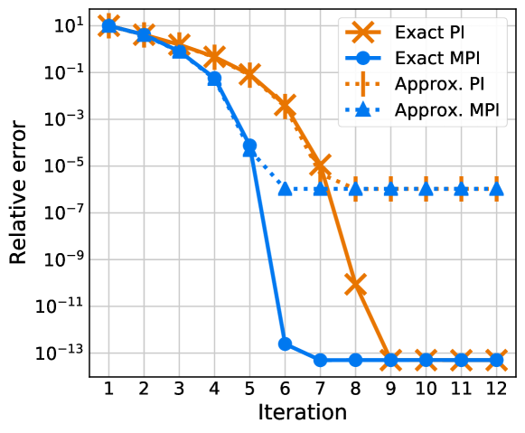
Figure 1: Relative value error $\|P_{k}-P^{*}\|/\|P^{*}\|$ vs iteration count $k$ using PI and MPI on the inertial mass control problem.

6.2 Randomized examples

Next we apply the exact and approximate PI algorithms on $10000$ unique problem instances in a Monte Carlo-style approach, where problem data was generated randomly with $n=4$, $m=2$, entries of $A$ drawn from $\mathcal{N}(0,1)$ and $A$ scaled so $\rho(A)\sim\text{Unif}([0,2])$, entries of $B$ drawn from $\text{Unif}([0,1])$, and $Q=U\Lambda U^{\intercal}\succ 0$ with $\Lambda$ diagonal with entries drawn from $\text{Unif}([0,1])$ and $U$ orthogonal by taking the QR-factorization of a square matrix with entries drawn from $\mathcal{N}(0,1)$, where we denote the uniform distribution on the interval $[a,b]$ by $\text{Unif}([a,b])$ and the multivariate Gaussian distribution with mean $\mu$ and variance $\Sigma$ by $\mathcal{N}(\mu,\Sigma)$. We used a small process noise covariance of $W=10^{-6}I_{4}$ to avoid unstable iterates due to excessive data-based approximation error of $H$, over all problem instances. All initial gains $K_{0}$ were chosen by perturbing the optimal gain $K^{*}$ in a random direction such that the initial relative error $\|P_{k}-P^{*}\|/\|P^{*}\|=10$. For the approximate algorithms, we used the hyperparameters $\ell=100$, $\mathcal{X}_{0}=\mathcal{N}(0,I_{2})$, $\mathcal{U}_{t}=\mathcal{N}(0,I_{2})$ for $t=0,1,\ldots,\ell$.

In Figures LABEL:fig:plot_error_monte_carlo_true_scatter, LABEL:fig:plot_error_monte_carlo_false_scatter, LABEL:fig:plot_error_monte_carlo_false_scatter_on we plot the relative value error $\|P_{k}-P^{*}\|/\|P^{*}\|$ over iterations, and each scatter point represents a unique Monte Carlo sample, i.e. a unique problem instance, initial gain, and rollout. Each plot shows the empirical distribution of errors at the iteration count $k$ labeled in the subplot titles above each plot. The x-axis is the spectral radius of $A$ which characterizes open-loop stability.

• Figure LABEL:fig:plot_error_monte_carlo_true_scatter shows the results of the exact algorithms i.e. Algorithm 1.

• Figure LABEL:fig:plot_error_monte_carlo_false_scatter shows the results of the offline approximate algorithms i.e. Algorithm 4 (OFF).

• Figure LABEL:fig:plot_error_monte_carlo_false_scatter_on shows the results of the online approximate algorithms i.e. Algorithm 4 (ON).

In sub-Figures LABEL:fig:plot_error_monte_carlo_true_scatter (b), LABEL:fig:plot_error_monte_carlo_false_scatter (b), LABEL:fig:plot_error_monte_carlo_false_scatter_on (b), scatter points lying below 1.0 on the y-axis indicate that the midpoint method achieves lower error than the standard method on the same problem instance.

From Figure LABEL:fig:plot_error_monte_carlo_true_scatter (a), it is clear that MPI achieves extremely fast convergence to the optimal gain, with the relative error being less than $10^{-13}$, essentially machine precision, on almost all problem instances after just 5 iterations. From Figure LABEL:fig:plot_error_monte_carlo_true_scatter (b), we see that MPI achieves significantly lower error than PI on iteration counts $2,3,4,5$ for almost all problem instances. The relative differences in error on iteration counts $6,7$ are due to machine precision error and are negligible for the purposes of comparison i.e. after 6 iterations both algorithms have effectively converged to the same solution.

We observe very similar results using the approximate algorithms. From Figure LABEL:fig:plot_error_monte_carlo_false_scatter (a), it is clear that AMPI achieves extremely fast convergence to a good approximation of the optimal gain, with the relative error being less than $10^{-6}$ on almost all problem instances after just 4 iterations. From Figure LABEL:fig:plot_error_monte_carlo_false_scatter (b), we see that AMPI achieves significantly lower error than API on iteration counts $2,3,4,5$ for almost all problem instances; recall that Algorithm 4 takes a standard PI step on the first iteration, explaining the identical performance on $k=1$. Similar trends are observed in Figure LABEL:fig:plot_error_monte_carlo_false_scatter_on with the online variant (ON), but the variation is much greater. Nevertheless, AMPI provides a clear advantage on iteration counts $2,3,4,5$, beating API in terms of relative error most of the time.

fig:plot_error_monte_carlo_true_scatter [Relative error using MPI]
 
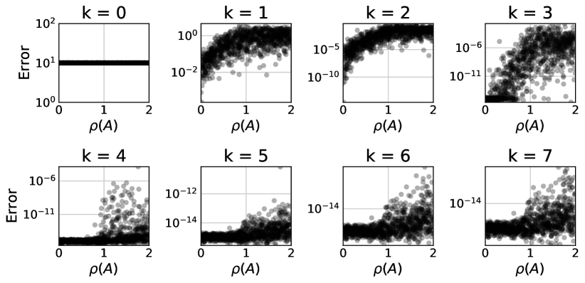
[Ratio of relative errors using MPI/PI]

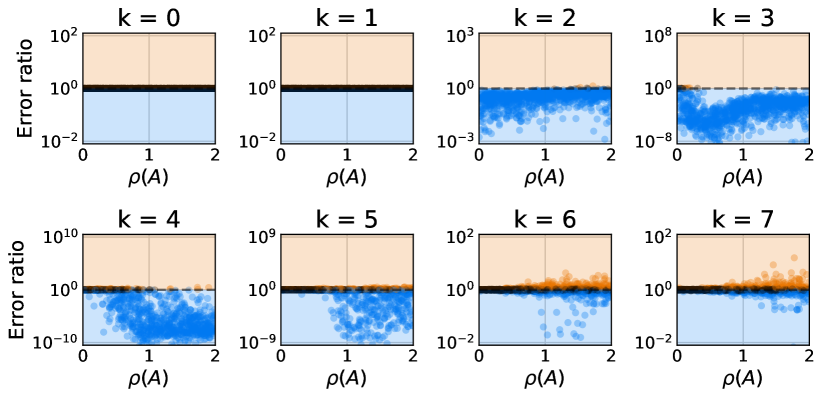
Figure 2: (a) Relative value error $\|P_{k}-P^{*}\|/\|P^{*}\|$ using MPI and (b) ratio of relative error using MPI divided by that using PI.

fig:plot_error_monte_carlo_false_scatter [Relative error using AMPI (OFF)]
 
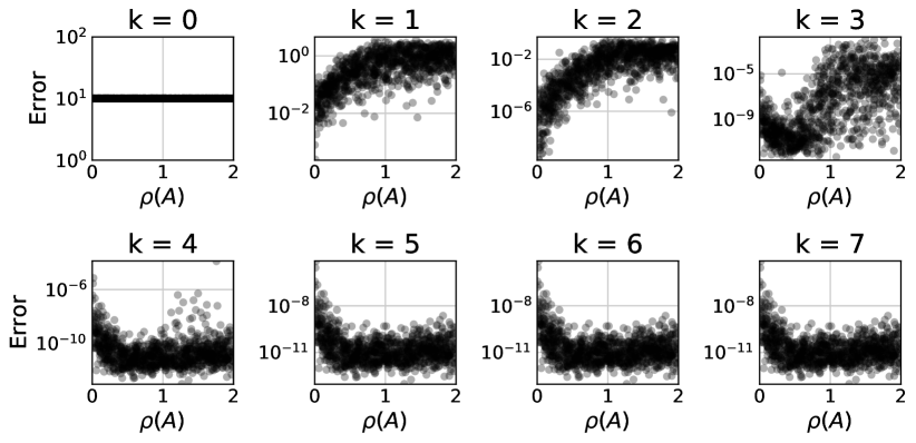
[Ratio of relative errors using AMPI/API (OFF)]

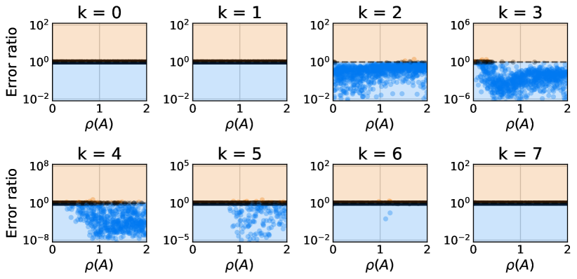
Figure 3: (a) Relative value error $\|P_{k}-P^{*}\|/\|P^{*}\|$ using AMPI and (b) ratio of relative error using AMPI divided by that using API, all with the offline algorithm variant (OFF).

fig:plot_error_monte_carlo_false_scatter_on [Relative error using AMPI (ON)]
 
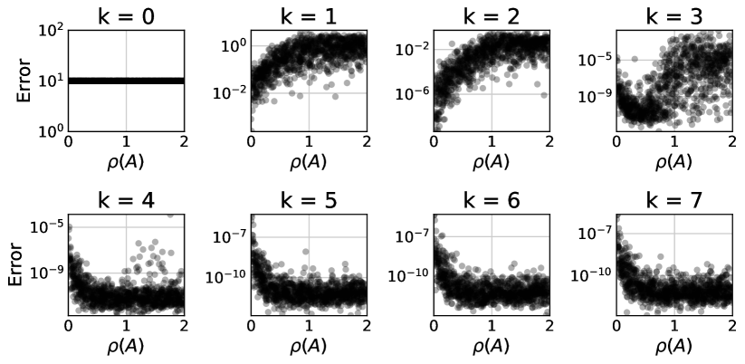
[Ratio of relative errors using AMPI/API (ON)]

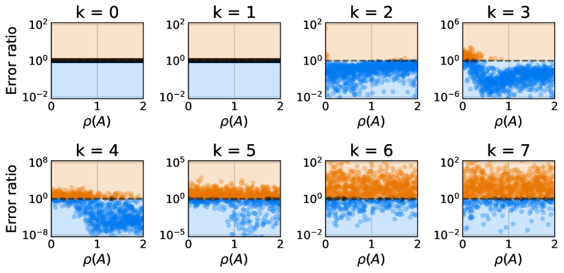
Figure 4: (a) Relative value error $\|P_{k}-P^{*}\|/\|P^{*}\|$ using AMPI and (b) ratio of relative error using AMPI divided by that using API, all with the offline algorithm variant (ON).

7 Conclusions and future work

Empirically, we found that regardless of the stabilizing initial policy chosen, convergence to the optimum always occurred when using the exact midpoint method. Likewise, we also found that approximate midpoint and standard PI converge to the same approximately optimal policy, and hence value matrix $P$, after enough iterations when evaluated on the same fixed off-policy rollout data $\mathcal{D}$. We conjecture that such robust, finite-data convergence properties can be proven rigorously, which we leave to future work.

This algorithm is perhaps most useful in the regime of practical problems in the online setting where it is relatively expensive to collect data and relatively cheap to perform the computations required to execute the updates. In such scenarios, the goal is to converge in as few iterations as possible, and MPI shows a clear advantage. Both the exact and approximate midpoint PI incur a computation cost double that of their standard PI counterparts. Theoretically, the faster cubic convergence rate of MPI over the quadratic convergence rate of PI should dominate this order constant (2$\times$) cost with sufficiently many iterations. However, unfortunately, due to finite machine precision, the total number of useful iterations that increase the precision of the optimal policy is limited, and the per-iteration cost largely counteracts the faster over-iteration convergence of MPI. This phenomenon becomes even more apparent in the model-free case where the “noise floor” is even higher. However, this disadvantage may be reduced by employing iterative Lyapunov equation solvers in Algorithm 1 or iterative (recursive) least-squares solvers in Algorithm 4 and warm-starting the midpoint equation with the Newton solution. Furthermore, the benefit of the faster convergence of the midpoint PI may become more important in extensions to nonlinear systems, where the order constants in Propositions 4.1 and 5.1 are smaller.

The current methodology is certainty-equivalent in the sense that we treat the estimated value functions as correct. Future work will explore ways to estimate and account for uncertainty in the value function estimate explicitly to minimize regret risk in the initial transient stage of learning when the amount of information is low and uncertainty is high.

References

- [Abbasi-Yadkori et al.(2019)Abbasi-Yadkori, Lazic, and Szepesvári] Yasin Abbasi-Yadkori, Nevena Lazic, and Csaba Szepesvári. Model-free linear quadratic control via reduction to expert prediction. In The 22nd International Conference on Artificial Intelligence and Statistics, pages 3108–3117, 2019.
- [Al-Tamimi et al.(2007)Al-Tamimi, Lewis, and Abu-Khalaf] Asma Al-Tamimi, Frank L Lewis, and Murad Abu-Khalaf. Model-free Q-learning designs for linear discrete-time zero-sum games with application to H-infinity control. Automatica, 43(3):473–481, 2007.
- [Anderson(1978)] Brian DO Anderson. Second-order convergent algorithms for the steady-state Riccati equation. International Journal of Control, 28(2):295–306, 1978.
- [Anderson and Moore(2007)] Brian DO Anderson and John B Moore. Optimal control: linear quadratic methods. Courier Corporation, 2007.
- [Argyros and Chen(1993)] Ioannis K Argyros and Dong Chen. Results on the chebyshev method in banach spaces. Proyecciones (Antofagasta, On line), 12(2):119–128, 1993.
- [Babajee and Dauhoo(2006)] D.K.R. Babajee and M.Z. Dauhoo. An analysis of the properties of the variants of Newton’s method with third order convergence. Applied Mathematics and Computation, 183(1):659 – 684, 2006. ISSN 0096-3003. https://doi.org/10.1016/j.amc.2006.05.116. URL \urlhttp://www.sciencedirect.com/science/article/pii/S0096300306006011.
- [Bellman(1959)] R.E. Bellman. Dynamic Programming. Dover paperback edition (2003). Princeton University Press, 1959. ISBN 0486428095.
- [Bertsekas et al.(1995)Bertsekas, Bertsekas, Bertsekas, and Bertsekas] Dimitri P Bertsekas, Dimitri P Bertsekas, Dimitri P Bertsekas, and Dimitri P Bertsekas. Dynamic programming and optimal control, volume 1. Athena scientific Belmont, MA, 1995.
- [Bradtke et al.(1994)Bradtke, Ydstie, and Barto] Steven J Bradtke, B Erik Ydstie, and Andrew G Barto. Adaptive linear quadratic control using policy iteration. In Proceedings of 1994 American Control Conference-ACC’94, volume 3, pages 3475–3479. IEEE, 1994.
- [Bu et al.(2020)Bu, Mesbahi, and Mesbahi] J. Bu, A. Mesbahi, and M. Mesbahi. LQR via first order flows. In 2020 American Control Conference (ACC), pages 4683–4688, 2020. 10.23919/ACC45564.2020.9147853.
- [Bu et al.(2019)Bu, Ratliff, and Mesbahi] Jingjing Bu, Lillian J Ratliff, and Mehran Mesbahi. Global convergence of policy gradient for sequential zero-sum linear quadratic dynamic games. arXiv preprint arXiv:1911.04672, 2019.
- [Coppens and Patrinos(2020)] Peter Coppens and Panagiotis Patrinos. Sample complexity of data-driven stochastic LQR with multiplicative uncertainty. arXiv preprint arXiv:2005.12167, 2020.
- [Coppens et al.(2020)Coppens, Schuurmans, and Patrinos] Peter Coppens, Mathijs Schuurmans, and Panagiotis Patrinos. Data-driven distributionally robust LQR with multiplicative noise. In Learning for Dynamics and Control, pages 521–530. PMLR, 2020.
- [Cuyt and Rall(1985)] Annie AM Cuyt and Louis B Rall. Computational implementation of the multivariate halley method for solving nonlinear systems of equations. ACM Transactions on Mathematical Software (TOMS), 11(1):20–36, 1985.
- [Damm and Hinrichsen(2001)] Tobias Damm and Diederich Hinrichsen. Newton’s method for a rational matrix equation occurring in stochastic control. Linear Algebra and its Applications, 332:81–109, 2001.
- [Dean et al.(2018)Dean, Mania, Matni, Recht, and Tu] Sarah Dean, Horia Mania, Nikolai Matni, Benjamin Recht, and Stephen Tu. Regret bounds for robust adaptive control of the linear quadratic regulator. In Advances in Neural Information Processing Systems, pages 4188–4197, 2018.
- [Dean et al.(2019)Dean, Mania, Matni, Recht, and Tu] Sarah Dean, Horia Mania, Nikolai Matni, Benjamin Recht, and Stephen Tu. On the sample complexity of the linear quadratic regulator. Foundations of Computational Mathematics, Aug 2019. ISSN 1615-3383.
- [Deuflhard(2012)] Peter Deuflhard. A short history of Newton’s method. Documenta Mathematica, pages 25–30, 2012.
- [Fazel et al.(2018)Fazel, Ge, Kakade, and Mesbahi] Maryam Fazel, Rong Ge, Sham Kakade, and Mehran Mesbahi. Global convergence of policy gradient methods for the linear quadratic regulator. In Proceedings of the 35th International Conference on Machine Learning, volume 80 of Proceedings of Machine Learning Research, pages 1467–1476. PMLR, 10–15 Jul 2018.
- [Freiling and Hochhaus(2004)] G Freiling and A Hochhaus. On a class of rational matrix differential equations arising in stochastic control. Linear Algebra and its Applications, 379:43 – 68, 2004. ISSN 0024-3795. https://doi.org/10.1016/S0024-3795(02)00651-1. URL \urlhttp://www.sciencedirect.com/science/article/pii/S0024379502006511. Special Issue on the Tenth ILAS Conference (Auburn, 2002).
- [Gravell and Summers(2020)] Benjamin Gravell and Tyler Summers. Robust learning-based control via bootstrapped multiplicative noise. In Proceedings of the 2nd Conference on Learning for Dynamics and Control, volume 120 of Proceedings of Machine Learning Research, pages 599–607. PMLR, 10–11 Jun 2020. URL \urlhttps://proceedings.mlr.press/v120/gravell20a.html.
- [Gravell et al.(2021a)Gravell, Esfahani, and Summers] Benjamin Gravell, Peyman Mohajerin Esfahani, and Tyler Summers. Learning optimal controllers for linear systems with multiplicative noise via policy gradient. IEEE Transactions on Automatic Control, 66(11):5283–5298, 2021a. 10.1109/TAC.2020.3037046.
- [Gravell et al.(2021b)Gravell, Ganapathy, and Summers] Benjamin Gravell, Karthik Ganapathy, and Tyler Summers. Policy iteration for linear quadratic games with stochastic parameters. IEEE Control Systems Letters, 5(1):307–312, 2021b. 10.1109/LCSYS.2020.3001883.
- [Guo and Laub(2000)] Chun-Hua Guo and Alan J Laub. On a Newton-like method for solving algebraic Riccati equations. SIAM Journal on Matrix Analysis and Applications, 21(2):694–698, 2000.
- [Gutiérrez and Hernández(2001)] J. M. Gutiérrez and M. A. Hernández. An acceleration of Newton’s method: Super-Halley method. Appl. Math. Comput., 117(2–3):223–239, January 2001. ISSN 0096-3003. 10.1016/S0096-3003(99)00175-7. URL \urlhttps://doi.org/10.1016/S0096-3003(99)00175-7.
- [Hernández-Verón and Romero(2018)] Miguel Angel Hernández-Verón and N Romero. Solving symmetric algebraic Riccati equations with high order iterative schemes. Mediterranean Journal of Mathematics, 15(2):51, 2018.
- [Hewer(1971)] G Hewer. An iterative technique for the computation of the steady state gains for the discrete optimal regulator. IEEE Transactions on Automatic Control, 16(4):382–384, 1971.
- [Homeier(2004)] H.H.H Homeier. A modified newton method with cubic convergence: the multivariate case. Journal of Computational and Applied Mathematics, 169(1):161 – 169, 2004. ISSN 0377-0427. https://doi.org/10.1016/j.cam.2003.12.041. URL \urlhttp://www.sciencedirect.com/science/article/pii/S0377042703010215.
- [Jansch-Porto et al.(2020)Jansch-Porto, Hu, and Dullerud] J. P. Jansch-Porto, B. Hu, and G. E. Dullerud. Convergence guarantees of policy optimization methods for markovian jump linear systems. In 2020 American Control Conference (ACC), pages 2882–2887, 2020. 10.23919/ACC45564.2020.9147571.
- [Kantorovich(1948)] LV Kantorovich. On newton’s method for functional equations. In Dokl. Akad. Nauk SSSR, volume 59, pages 1237–1240, 1948.
- [Kleinman(1968)] David Kleinman. On an iterative technique for Riccati equation computations. IEEE Transactions on Automatic Control, 13(1):114–115, 1968.
- [Kollerstrom(1992)] Nick Kollerstrom. Thomas Simpson and ‘Newton’s method of approximation’: an enduring myth. The British journal for the history of science, 25(3):347–354, 1992.
- [Krauth et al.(2019)Krauth, Tu, and Recht] Karl Krauth, Stephen Tu, and Benjamin Recht. Finite-time analysis of approximate policy iteration for the linear quadratic regulator. In Advances in Neural Information Processing Systems, pages 8512–8522, 2019.
- [Lagoudakis and Parr(2003)] Michail G. Lagoudakis and Ronald Parr. Least-squares policy iteration. J. Mach. Learn. Res., 4:1107–1149, December 2003. ISSN 1532-4435.
- [Luo et al.(2020)Luo, Yang, and Liu] B. Luo, Y. Yang, and D. Liu. Policy iteration Q-learning for data-based two-player zero-sum game of linear discrete-time systems. IEEE Transactions on Cybernetics, pages 1–11, 2020.
- [Madani(2002)] Omid Madani. On policy iteration as a Newton’s method and polynomial policy iteration algorithms. In AAAI/IAAI, pages 273–278, 2002.
- [Mania et al.(2019)Mania, Tu, and Recht] Horia Mania, Stephen Tu, and Benjamin Recht. Certainty equivalent control of LQR is efficient. ArXiv, abs/1902.07826, 2019.
- [Nedzhibov(2002)] Gyurhan Nedzhibov. On a few iterative methods for solving nonlinear equations. Application of mathematics in engineering and economics, 28:1–8, 2002.
- [Newton(1711)] Isaac Newton. De analysi per aequationes numero terminorum infinitas. 1711.
- [Oymak and Ozay(2019)] Samet Oymak and Necmiye Ozay. Non-asymptotic identification of LTI systems from a single trajectory. In 2019 American Control Conference (ACC), pages 5655–5661. IEEE, 2019.
- [Puterman and Brumelle(1979)] Martin L. Puterman and Shelby L. Brumelle. On the convergence of policy iteration in stationary dynamic programming. Mathematics of Operations Research, 4(1):60–69, 1979. ISSN 0364765X, 15265471. URL \urlhttp://www.jstor.org/stable/3689239.
- [Raphson(1702)] Joseph Raphson. Analysis aequationum universalis: seu ad aequationes algebraicas resolvendas methodus generalis, & expedita, ex nova infinitarum serierum methodo, deducta ac demonstrata, volume 1. Typis TB prostant venales apud A. & I. Churchill, 1702.
- [Selby(1974)] Samuel M Selby. CRC standard mathematical tables, 1974.
- [Simpson(1740)] Thomas Simpson. Essays on Several Curious and Useful Subjects, in Speculative and Mix’d Mathematicks. H. Woodfall, 1740.
- [Traub(1964)] Joe Fred Traub. Iterative methods for the solution of equations. 1964.
- [Tyrtyshnikov(2012)] Eugene E Tyrtyshnikov. A brief introduction to numerical analysis. Springer Science & Business Media, 2012.
- [Zhang et al.(2019)Zhang, Yang, and Basar] Kaiqing Zhang, Zhuoran Yang, and Tamer Basar. Policy optimization provably converges to Nash equilibria in zero-sum linear quadratic games. In Advances in Neural Information Processing Systems, pages 11598–11610, 2019.