Gauge couplings evolution from the Standard Model, through Pati-Salam theory, into $\mathrm{E}_{8}$ unification of families and forces

Abstract

We explore the potential of ultimate unification of the Standard Model matter and gauge sectors into a single $E_{8}$ superfield in ten dimensions via an intermediate Pati-Salam gauge theory. Through a consistent realisation of a $\mathbb{T}^{6}/(\mathbb{Z}_{6}\times\mathbb{Z}_{2})$ orbifolding procedure accompanied by the Wilson line breaking mechanism and Renormalisation Group evolution of gauge couplings, we have established several benchmark scenarios for New Physics that are worth further phenomenological exploration.

I Introduction

Grand Unified Theories (GUTs) aim to unify the three independent gauge interactions of the Standard Model (SM) into a single one. Among the simplest ways to achieve this is via an $SU(5)$ gauge symmetry Georgi:1974sy . One can also extend the gauge symmetry to unify all the SM fermions of a single family into one $SO(10)$ representation Fritzsch:1974nn . Enlarging the gauge group even further into $E_{6}$, one could unify the SM Higgs sector and a full family of fermions into a single representation King:2005my by means of the simple ${\cal N}=1$ supersymmetry (SUSY).

Such a step-by-step enlarging of the gauge symmetry group can be studied through its Dynkin diagram and is known to follow the exceptional chain Buchmuller:1985rc ; Koca:1982zi ,

$$SU(3)_{C}\times SU(2)_{L}\times U(1)_{Y}\subset SU(5)\subset SO(10)\subset E_{6}\subset E_{7}\subset E_{8}\,.$$ (1)

Note, the group $E_{8}$ is the largest group of the chain and is specially relevant as its adjoint representation $(\textbf{248})$ is the same as the fundamental one Slansky:1981yr . This suggests that the SM gauge fields can be in principle unified with the SM fermions provided that a maximal $\mathcal{N}=4$ SUSY is realised. Furthermore, it also provides an $SU(3)$ flavor (or family) symmetry as a coset of $E_{8}$ to $E_{6}$ reduction.

There is a plethora of models in the literature that aim to build GUTs including flavor symmetries King:2001uz ; King:2017guk ; Hagedorn:2010th ; Antusch:2014poa ; Bjorkeroth:2015ora ; Bjorkeroth:2015uou ; Bjorkeroth:2017ybg ; deAnda:2017yeb ; CarcamoHernandez:2020owa ; Morais:2020ypd ; Morais:2020odg ; Camargo-Molina:2016yqm ; Camargo-Molina:2017kxd ; Camargo-Molina:2016yqm ; Camargo-Molina:2016bwm and extra dimensions (EDs), Altarelli:2008bg ; Burrows:2009pi ; Burrows:2010wz ; deAnda:2018oik ; Altarelli:2006kg ; Adulpravitchai:2010na ; Adulpravitchai:2009id ; Asaka:2001eh ; deAnda:2019jxw ; deAnda:2018ecu ; deAnda:2018yfp ). In order to achieve viability, most require a number of independent groups and quite a large number of fields. As alluded above, the group $E_{8}$ seems to be a good bet for a complete unification of SM vectors, fermions and scalars and has indeed been widely studied both in the context of string theory Ibanez:1987pj ; Parr:2020oar and within the framework of quantum field theory (QFT) Adler:2002yg ; Adler:2004uj ; Garibaldi:2016zgm ; Thomas:1985be ; Konshtein:1980km ; Baaklini:1980fv ; Baaklini:1980uq ; Barr:1987pu ; Bars:1980mb ; Koca:1981xd ; Mahapatra:1988gc ; Ong:1984ej ; Camargo-Molina:2016yqm ; Olive:1982ai .

The first challenge posed by $E_{8}$ is that it is a real group (as is extended SUSY) while the SM requires chiral representations. A way forward is to assume the existence of extra dimensions which are orbifolded in such a way that, after their compactification, the massless chiral representations containing the SM fermion sectors remain. Furthermore, extended SUSY can also be generated from the EDs ArkaniHamed:2001tb ; Brink:1976bc . A big challenge is to avoid the presence of too many massless states in the low-energy limit of the theory typically originating by an orbifolding procedure of $E_{8}$. A consistent resolution may be found by a combination of orbifolding and the Wilson line symmetry-breaking mechanism, also associated to the specific orbifold structure, providing a reduction of the symmetry group and generation of large masses for many of the unobserved states.

One of the main requirements for a consistent GUT is gauge couplings unification, i.e., when the SM gauge couplings are evolved from their measured values at the electroweak (EW) scale up to the high-energy scales and they match into a single coupling of a unified gauge group. Recently Aranda:2020noz ; Aranda:2020zms , some of us presented a framework where the $E_{8}$ gauge symmetry with $\mathcal{N}=1$ SUSY is considered in 10d corresponding to an extended $\mathcal{N}=4$ SUSY in 4d, where the EDs are orbifolded so that after the compactification stage only simple SUSY and Pati-Salam symmetry remain Pati:1973uk .

In this paper, we study a particular realisation of the GUT with $E_{8}$ gauge symmetry in 10d, where the full SM (Higgs, gauge, fermion) field content is unified into a single $E_{8}$ gauge superfield. Through the $\mathbb{T}^{6}/(\mathbb{Z}_{6}\times\mathbb{Z}_{2})$ orbifold, the $E_{8}$ symmetry is broken down into $SU(4)_{PS}\times SU(2)_{L}\times SU(2)_{R}\times U(1)_{X}\times U(1)_{F}\times SU(2)_{F}$. In order to consistently derive the 4d Pati-Salam theory from $E_{8}$ in 10d, the ED compactification procedure invokes the presence of several extra fields for the model to be anomaly free at every step. Thus, we assume the existence of additional chiral superfields, consistent with the $E_{8}$ symmetry, so that the anomalies are manifestly canceled at the Pati-Salam level. The symmetry is further broken down to the SM one through Wilson lines.

The SM gauge and matter sectors originate from a single gauge superfield and remain massless up to the EW symmetry breaking scale. The additional chiral fields have arbitrary masses and thus may not be present at low energies. In this work, we study different benchmark scenarios of New Physics where some of the fields survive below the compactification scale and provide important contributions to the renormalization group (RG) evolution of the gauge couplings necessary to achieve the exact gauge couplings unification below the Planck scale.

The layout of the paper is as follows: In Sec. II we show the basics of the orbifolding mechanism employed in this work. In Sec. III we demonstrate how the specific $\mathbb{T}_{6}/(\mathbb{Z}_{6}\times\mathbb{Z}_{2})$ orbifold breaks the $E_{8}$ gauge symmetry and SUSY in 10d. In Sec. IV we introduce the extra superfields that are needed to cancel anomalies at the Pati-Salam level. In Sec. V we present the benchmark scenarios relevant for further explorations of New Physics phenomenology where the exact gauge couplings unification is achieved. Finally, in Sec. VI the basic conclusions are summarised.

II Orbifolding

Let us start by considering a theory in 10d spacetime with $\mathcal{N}=1$ SUSY. Six extra spatial dimensions are assumed to be orbifolded as $\mathbb{T}^{6}/F$, where $F$ is a discrete subgroup of the extra dimensional Poincarè symmetry $O(6)\ltimes T^{6}$, such that $O(6)\simeq SO(6)\times\mathbb{Z}_{2}\simeq SU(4)\times\mathbb{Z}_{2}$ is the rotation group, while $T^{6}$ is the translation group. The translation group is modded by the lattice vectors $\Gamma=\mathbb{Z}^{6}$ compactifying it as $\mathbb{R}^{6}\to\mathbb{T}^{6}\simeq\mathbb{R}^{6}/\Gamma$ into a 6d torus. The group $F$ must leave the lattice invariant, i.e. $F\Gamma=\Gamma$. In order to preserve simple ${\cal N}=1$ SUSY after orbifold compactification, one should leave an invariant $U(1)$ subgroup of the rotations, therefore $F\subset SU(3)$ Dixon:1985jw ; Dixon:1986jc .

A simple orbifolding that preserves $\mathcal{N}=1$ SUSY reads

$$F\simeq\mathbb{Z}_{N}\subset SU(3)\,,$$ (2)

with a positive integer $N$, where a generic $\mathbb{Z}_{N}$ orbifolding can be defined by identifying

$$(x,z_{1},z_{2},z_{3})\sim(x,\omega_{1}z_{1},\omega_{2}z_{2},\omega_{3}z_{3})\,,\qquad\omega_{i}\equiv e^{2i\pi n_{i}/N}\,,$$

$${\cal V}(x,z_{1},z_{2},z_{3})=R(\omega_{1},\omega_{2},\omega_{3}){\cal V}(x,\omega_{1}z_{1},\omega_{2}z_{2},\omega_{3}z_{3})\,.$$ (3)

Here, $R$ corresponds to a representation of the $\mathbb{Z}_{N}$ rotation acting on the $10$d vector superfield ${\cal V}$. Such a transformation would belong to $SU(3)$ and preserve SUSY as long as

$$n_{1}+n_{2}+n_{3}=0\mod 2N\,,$$ (4)

as fermions rotate twice as slow GrootNibbelink:2017luf .

Considering only an Abelian orbifolding that preserves $\mathcal{N}=1$ SUSY, the most general one reads as $F\simeq\mathbb{Z}_{N}\times\mathbb{Z}_{M}\subset SU(3)$, where $N,M$ are positive integers deAnda:2019anb ; Fischer:2012qj ; Fischer:2013qza . If the boundary condition that breaks the gauge group is imposed, the orbifolding must be accompanied by an $E_{8}\supset U(1)_{f}\supset\mathbb{Z}_{N}$ transformation. As a result, the decomposed $10$d superfield is transformed as follows

$$\begin{split}V(x,z_{1},z_{2},z_{3})&=e^{2i\pi q^{f}_{a}/N}V(x,\omega_{1}z_{1},\omega_{2}z_{2},\omega_{3}z_{3}),\\ \phi^{i}(x,z_{1},z_{2},z_{3})&=\omega_{i}e^{2i\pi q^{f}_{a}/N}\phi^{i}(x,\omega_{1}z_{1},\omega_{2}z_{2},\omega_{3}z_{3}),\end{split}$$ (5)

where $q_{a}^{f}$ is the $U(1)_{f}$ charge of the corresponding representation. Here, $V$ lies in the adjoint representation of the unbroken gauge group, while the light chiral superfields $\phi_{i}$ belong to the corresponding fundamental representation with charge $q^{f}_{a}=-n_{i}\mod N$. The desired light fields are then specified by an appropriate choice of $n_{i}$. This fully determines the orbifolding procedure.

The underlined gauge symmetry can be broken and its rank reduced by adding a gauge transformation to the EDs translations through the so-called Wilson line mechanism. The latter generates a mass splitting similar to the one a Vacuum Expectation Value (VEVs) would generate. It is therefore usual to parametrize this symmetry breaking by an effective VEV. It should be remembered that it is not actually a VEV, as it does not come from the minimization of a potential, but from the ED profiles of the fields, determined by boundary conditions. In consistency with the orbifold boundary conditions, the effective VEVs should obey the rotation-translation commutation relations coming from the Poincarè algebra and hence emerge in chiral supermultiplets that have a zero mode. An effective potential for the fields is obtained by integrating out all the other fields (for more details, see e.g. Refs. Hosotani:1983xw ; Hosotani:1983vn ; Hosotani:2004wv ; Hosotani:2004ka ; Haba:2004qf ; Haba:2002py ).

III The $\mathbb{T}^{6}/(\mathbb{Z}_{6}\times\mathbb{Z}_{2})$ orbifold with $E_{8}$

Now, we consider an $E_{8}$ gauge theory in 10d spacetime. The $E_{8}$ gauge symmetry has rank $8$ and the orbifolding must preserve the rank-4 SM gauge symmetry, $SU(3)_{C}\times SU(2)_{L}\times U(1)_{Y}$. In this work, we employ the following decomposition Slansky:1981yr

$$\begin{split}E_{8}&\supset SO(10)\times U(1)_{X^{\prime}}\times SU(3)_{F}\\ &\quad\supset SO(10)\times U(1)_{X^{\prime}}\times U(1)_{F}\times SU(2)_{F}\\ &\quad\supset G_{PS}\equiv SU(4)_{PS}\times SU(2)_{L}\times SU(2)_{R}\times U(1)_{X^{\prime}}\times U(1)_{F}\times SU(2)_{F}\,,\end{split}$$ (6)

and consider the $T^{6}/(\mathbb{Z}_{6}\times\mathbb{Z}_{2})$ orbifold whose compactification triggers the breaking $E_{8}\to G_{PS}$ i.e. featuring a Pati-Salam SUSY theory and a flavor $U(1)_{F}\times SU(2)_{F}$ symmetry in 4d. Subsequent reduction of this symmetry occurs in the following steps,

$$SU(4)_{PS}\to SU(3)_{C}\times U(1)_{B-L}\,,\qquad SU(2)_{R}\to U(1)_{T_{3}^{R}}\,,$$ (7)

$$SU(4)_{PS}\times SU(2)_{R}\to SU(3)_{C}\times U(1)_{Y}\times U(1)_{X}\,,$$

with

$$q_{Y}=6q_{T_{3}^{R}}+3q_{B-L}\,,\qquad q_{X}=4Q_{T_{3}^{R}}-3q_{B-L}\,,$$ (8)

where one recovers the color $SU(3)_{C}$ and hypercharge $U(1)_{Y}$ groups of the SM.

The orbifold boundary conditions which provide such a breaking pattern read

$$\mathbb{Z}_{6}:\ \phi\to e^{2i\pi q_{X^{\prime}}/6}\phi\,,\ \ \ \mathbb{Z}_{2}:\ \phi\to e^{2i\pi(q_{Y}+q_{T_{8}^{F}})/2}\phi\,,$$ (9)

with the orbifold transformations

$$\begin{split}(x,z_{1},z_{2},z_{3})&\sim(x,\alpha^{2}z_{1},\alpha^{5}z_{2},\alpha^{5}z_{3})\,,\\ (x,z_{1},z_{2},z_{3})&\sim(x,-z_{1},-z_{2},(-1)^{2}z_{3})\,,\end{split}$$ (10)

where $\alpha=e^{2i\pi/6}$ and $-1=e^{2i\pi/2}$. The breaking described in the first line of eq. 6 is achieved by the boundary condition given by $q_{X^{\prime}}/6$. It is further broken to the second line by the boundary condition $q_{T_{8}^{F}}/2$. The third line is achieved by further appyling $q_{Y}/2$. The above conditions enable us to decompose the 248 representation of $E_{8}$ into the representations of unbroken $G_{PS}$ symmetry summarised in Table 1, together with the corresponding charges (for a better presentation we color code the representations containing SM fermions, right handed neutrinos, SM Higgses, gauge fields in the adjoint, mirror fermions, mirror Higgses, flavons, leptoquarks and vector-like triplets).

	$V$	$\phi_{1}$	$\phi_{2}$	$\phi_{3}$
$\mathcal{V}_{{\color[rgb]{1,0,1}(\textbf{15},\textbf{1},\textbf{1},0,0,\textbf{1})}}$	$1,1$	$\alpha^{2},-1$	$\alpha^{5},-1$	$\alpha^{5},1$
$\mathcal{V}_{{\color[rgb]{1,0,1}(\textbf{1},\textbf{3},\textbf{1},0,0,\textbf{1})}}$	$1,1$	$\alpha^{2},-1$	$\alpha^{5},-1$	$\alpha^{5},1$
$\mathcal{V}_{{\color[rgb]{1,0,1}(\textbf{1},\textbf{1},\textbf{3},0,0,\textbf{1})}}$	$1,1$	$\alpha^{2},-1$	$\alpha^{5},-1$	$\alpha^{5},1$
$\mathcal{V}_{{\color[rgb]{1,0,1}(\textbf{1},\textbf{1},\textbf{1},0,0,\textbf{1})}}$	$1,1$	$\alpha^{2},-1$	$\alpha^{5},-1$	$\alpha^{5},1$
$\mathcal{V}_{{\color[rgb]{1,0,1}(\textbf{1},\textbf{1},\textbf{1},0,0,\textbf{3})}}$	$1,1$	$\alpha^{2},-1$	$\alpha^{5},-1$	$\alpha^{5},1$
$\mathcal{V}_{{\color[rgb]{1,0,1}(\textbf{1},\textbf{1},\textbf{1},0,0,\textbf{1})}}$	$1,1$	$\alpha^{2},-1$	$\alpha^{5},-1$	$\alpha^{5},1$
$\mathcal{V}_{{\color[rgb]{.75,.5,.25}(\textbf{1},\textbf{1},\textbf{1},0,-3,\textbf{2})}}$	$1,-1$	$\alpha^{2},1$	$\alpha^{5},1$	$\alpha^{5},-1$
$\mathcal{V}_{{\color[rgb]{.75,.5,.25}(\textbf{1},\textbf{1},\textbf{1},3,0,\textbf{2})}}$	$1,-1$	$\alpha^{2},1$	$\alpha^{5},1$	$\alpha^{5},-1$
$\mathcal{V}_{(\textbf{6},\textbf{2},\textbf{2},0,0,\textbf{1})}$	$1,-1$	$\alpha^{2},1$	$\alpha^{5},1$	$\alpha^{5},-1$
$\mathcal{V}_{(\textbf{4},\textbf{2},\textbf{1},-3,0,\textbf{1})}$	$\alpha^{3},-1$	$\alpha^{5},1$	$\alpha^{2},1$	$\alpha^{2},-1$
$\mathcal{V}_{(\bar{\textbf{4}},\textbf{1},\textbf{2},-3,0,\textbf{1})}$	$\alpha^{3},1$	$\alpha^{5},-1$	$\alpha^{2},-1$	$\alpha^{2},1$
$\mathcal{V}_{(\bar{\textbf{4}},\textbf{2},\textbf{1},3,0,\textbf{1})}$	$\alpha^{3},-1$	$\alpha^{5},1$	$\alpha^{2},1$	$\alpha^{2},-1$
$\mathcal{V}_{(\textbf{4},\textbf{1},\textbf{2},3,0,\textbf{1})}$	$\alpha^{3},1$	$\alpha^{5},-1$	$\alpha^{2},-1$	$\alpha^{2},1$
$\mathcal{V}_{(\textbf{6},\textbf{1},\textbf{1},-2,1,\textbf{2})}$	$\alpha^{4},-1$	$1,1$	$\alpha^{3},1$	$\alpha^{3},-1$
$\mathcal{V}_{(\textbf{6},\textbf{1},\textbf{1},-2,-2,\textbf{1})}$	$\alpha^{4},1$	$1,-1$	$\alpha^{3},-1$	$\alpha^{3},1$
$\mathcal{V}_{(\textbf{6},\textbf{1},\textbf{1},2,-1,\textbf{2})}$	$\alpha^{2},-1$	$\alpha^{4},1$	$\alpha,1$	$\alpha,-1$
$\mathcal{V}_{(\textbf{6},\textbf{1},\textbf{1},2,2,\textbf{1})}$	$\alpha^{2},1$	$\alpha^{4},-1$	$\alpha,-1$	$\alpha,1$

	$V$	$\phi_{1}$	$\phi_{2}$	$\phi_{3}$
$\mathcal{V}_{{\color[rgb]{0,0,1}(\textbf{4},\textbf{2},\textbf{1},1,1,\textbf{2})}}$	$\alpha,1$	$\alpha^{3},-1$	$1,-1$	$1,1$
$\mathcal{V}_{{\color[rgb]{0,0,1}(\textbf{4},\textbf{2},\textbf{1},1,-2,\textbf{1})}}$	$\alpha,-1$	$\alpha^{3},1$	$1,1$	$1,-1$
$\mathcal{V}_{{\color[rgb]{0,0,1}(\bar{\textbf{4}},\textbf{1},\textbf{2},1,1,\textbf{2})}}$	$\alpha,-1$	$\alpha^{3},1$	$1,1$	$1,-1$
$\mathcal{V}_{{\color[rgb]{0,0,1}(\bar{\textbf{4}},\textbf{1},\textbf{2},1,-2,\textbf{1})}}$	$\alpha,1$	$\alpha^{3},-1$	$1,-1$	$1,1$
$\mathcal{V}_{{\color[rgb]{0,0.6,0}(\textbf{1},\textbf{2},\textbf{2},-2,1,\textbf{2})}}$	$\alpha^{4},1$	$1,-1$	$\alpha^{3},-1$	$\alpha^{3},1$
$\mathcal{V}_{{\color[rgb]{0,0.6,0}(\textbf{1},\textbf{2},\textbf{2},-2,-2,\textbf{1})}}$	$\alpha^{4},-1$	$1,1$	$\alpha^{3},1$	$\alpha^{3},-1$
$\mathcal{V}_{{\color[rgb]{.75,.5,.25}(\textbf{1},\textbf{1},\textbf{1},4,1,\textbf{2})}}$	$\alpha^{4},-1$	$1,1$	$\alpha^{3},1$	$\alpha^{3},-1$
$\mathcal{V}_{{\color[rgb]{.75,.5,.25}(\textbf{1},\textbf{1},\textbf{1},4,-2,\textbf{1})}}$	$\alpha^{4},1$	$1,-1$	$\alpha^{3},-1$	$\alpha^{3},1$
$\mathcal{V}_{{\color[rgb]{1,0,0}(\bar{\textbf{4}},\textbf{2},\textbf{1},-1,-1,\textbf{2})}}$	$\alpha^{5},1$	$\alpha,-1$	$\alpha^{4},-1$	$\alpha^{4},1$
$\mathcal{V}_{{\color[rgb]{1,0,0}(\bar{\textbf{4}},\textbf{2},\textbf{1},-1,2,\textbf{1})}}$	$\alpha^{5},-1$	$\alpha,1$	$\alpha^{4},1$	$\alpha^{4},-1$
$\mathcal{V}_{{\color[rgb]{1,0,0}(\textbf{4},\textbf{1},\textbf{2},-1,-1,\textbf{2})}}$	$\alpha^{5},-1$	$\alpha,1$	$\alpha^{4},1$	$\alpha^{4},-1$
$\mathcal{V}_{{\color[rgb]{1,0,0}(\textbf{4},\textbf{1},\textbf{2},-1,2,\textbf{1})}}$	$\alpha^{5},1$	$\alpha,-1$	$\alpha^{4},-1$	$\alpha^{4},1$
$\mathcal{V}_{{\color[rgb]{1,.5,0}(\textbf{1},\textbf{2},\textbf{2},2,-1,\textbf{2})}}$	$\alpha^{2},1$	$\alpha^{4},-1$	$\alpha,-1$	$\alpha,1$
$\mathcal{V}_{{\color[rgb]{1,.5,0}(\textbf{1},\textbf{2},\textbf{2},2,2,\textbf{1})}}$	$\alpha^{2},-1$	$\alpha^{4},1$	$\alpha,1$	$\alpha,-1$
$\mathcal{V}_{{\color[rgb]{.75,.5,.25}(\textbf{1},\textbf{1},\textbf{1},-4,-1,\textbf{2})}}$	$\alpha^{2},-1$	$\alpha^{4},1$	$\alpha,1$	$\alpha,-1$
$\mathcal{V}_{{\color[rgb]{.75,.5,.25}(\textbf{1},\textbf{1},\textbf{1},-4,2,\textbf{1})}}$	$\alpha^{2},1$	$\alpha^{4},-1$	$\alpha,-1$	$\alpha,1$

Table 1: The $\mathbb{Z}_{6}\times\mathbb{Z}_{2}$ orbifold charges of each $G_{PS}$ $\mathcal{N}=1$ superfield. Only the superfields with both charges equal to unity (the singlets $1,1$) have zero modes. The colors indicate where the different fields of interest are contained: SM fermions, right handed neutrinos, SM Higgses, gauge fields in the adjoint, mirror fermions, mirror Higgses, flavons, leptoquarks and vector-like triplets

The zero modes have the following representations of the residual symmetry group (recall they correspond to those with $1,1$ charges in Table 1):

$$\begin{split}V_{\mu}&:{\color[rgb]{1,0,1}(\textbf{15},\textbf{1},\textbf{1},0,0,\textbf{1})}+{\color[rgb]{1,0,1}(\textbf{1},\textbf{3},\textbf{1},0,0,\textbf{1})}+{\color[rgb]{1,0,1}(\textbf{1},\textbf{1},\textbf{3},0,0,\textbf{1})}\\ &\quad+{\color[rgb]{1,0,1}(\textbf{1},\textbf{1},\textbf{1},0,0,\textbf{1})}+{\color[rgb]{1,0,1}(\textbf{1},\textbf{1},\textbf{1},0,0,\textbf{1})}+{\color[rgb]{1,0,1}(\textbf{15},\textbf{1},\textbf{1},0,0,\textbf{3})},\\ \phi_{1}&:(\textbf{6},\textbf{1},\textbf{1},-2,1,\textbf{2})+{\color[rgb]{0,0.6,0}(\textbf{1},\textbf{2},\textbf{2},-2,-2,\textbf{1})}+{\color[rgb]{.75,.5,.25}(\textbf{1},\textbf{1},\textbf{1},4,1,\textbf{2})},\\ \phi_{2}&:{\color[rgb]{0,0,1}(\textbf{4},\textbf{2},\textbf{1},1,-2,\textbf{1})}+{\color[rgb]{0,0,1}(\bar{\textbf{4}},\textbf{1},\textbf{2},1,1,\textbf{2})},\\ \phi_{3}&:{\color[rgb]{0,0,1}(\textbf{4},\textbf{2},\textbf{1},1,1,\textbf{2})}+{\color[rgb]{0,0,1}(\bar{\textbf{4}},\textbf{1},\textbf{2},1,-2,\textbf{1})}.\end{split}$$ (11)

which can be named as

$$\begin{split}V_{\mu}&:{\color[rgb]{1,0,1}G_{\mu}}+{\color[rgb]{1,0,1}W^{L}_{\mu}}+{\color[rgb]{1,0,1}W^{R}_{\mu}}+{\color[rgb]{1,0,1}Z^{\prime}_{\mu}}+{\color[rgb]{1,0,1}Z^{F}_{\mu}}+{\color[rgb]{1,0,1}W^{F}_{\mu}},\\ \phi_{1}&:T+{\color[rgb]{0,0.6,0}h}+{\color[rgb]{.75,.5,.25}\Phi},\\ \phi_{2}&:{\color[rgb]{0,0,1}f}+{\color[rgb]{0,0,1}F^{c}},\\ \phi_{3}&:{\color[rgb]{0,0,1}F}+{\color[rgb]{0,0,1}f^{c}},\end{split}$$ (12)

where uppercase letters $T,F,\Phi$ are used to denote $SU(2)_{F}$ doublets and lowercase letters $f,h$ correspond to $SU(2)_{F}$ singlets.

In order to further break the intermediate symmetry group down to the SM, one could use each Wilson line to give an effective VEV to the SM singlet fields

$$\begin{split}\braket{\phi_{1}}&:{\color[rgb]{.75,.5,.25}\braket{\Phi}},\\ \braket{\phi_{2}}&:{\color[rgb]{0,0,1}\braket{F^{c}}},\\ \braket{\phi_{3}}&:{\color[rgb]{0,0,1}\braket{f^{c}}},\end{split}$$ (13)

where, in principle, one could choose an arbitrary scale for each effective VEV, as they come from the arbitrary Wilson lines and not from a potential. Their natural scale would be close to the compactification scale $\Lambda$. The effective VEV $\braket{{\color[rgb]{0,0,1}F^{c}}}=(\braket{{\color[rgb]{.5,0,.5}\tilde{\nu}^{c}_{2}}},\braket{{\color[rgb]{.5,0,.5}\tilde{\nu}^{c}_{3}}})$ and $\braket{{\color[rgb]{0,0,1}f^{c}}}=\braket{{\color[rgb]{.5,0,.5}\tilde{\nu}^{c}_{1}}}$ should be aligned in the SM singlets, i.e. the right-handed sneutrino. They are charged under $SU(4)_{PS}\times SU(2)_{R}\times U(1)_{X^{\prime}}\times U(1)_{F}\times SU(2)_{F}$ so their VEVs break it. However, they are neutral under a $U(1)_{N}$ whose charge is defined by

$$q_{N}=q_{X}+5q_{X^{\prime}}\,,$$ (14)

and therefore do not break it. Note that the VEV $\braket{{\color[rgb]{.75,.5,.25}\Phi}}=({\color[rgb]{.75,.5,.25}\braket{\varphi_{2}}},{\color[rgb]{.75,.5,.25}\braket{\varphi_{3}}})$ has a non-zero $q_{N}$ charge and hence breaks the remaining $U(1)_{N}$ symmetry yielding the SM gauge symmetry at low energies. Therefore, the complete geometrical breaking, involving the orbifold boundary conditions and Wilson lines, reduces $E_{8}\to G_{SM}\equiv SU(3)_{C}\times SU(2)_{L}\times U(1)_{Y}$ as desired.

IV Anomaly-canceling sector

We have shown that the orbifold breaks the $E_{8}$ symmetry down to the SM one leaving the desired SM field content. However, one has to ensure that any potential anomalies are cancelled at every symmetry breaking step. Let us discuss this point in more detail.

The rotation boundary conditions split the masses of different representations by integer multiples of the compactification scale $n\Lambda$. The Wilson lines split the masses by an effective VEV with scale $y\Lambda$, where $y$ is an arbitrary real parameter. The latter can, in principle, be as small as desired, generating a certain hierarchy between the scales. Therefore, one could think of the subsequential breaking $E_{8}\to G_{PS}\to G_{SM}$ at well-separated energy scales as a New Physics scenario potentially relevant for phenomenology.

The field content in the Pati-Salam phase would be composed of zero modes from Eq. (11). However, we can easily notice that this phase is not fully consistent as the field content generates gauge anomalies, while the SM phase is anomaly free. In order to resolve this issue, one can add more fields so that the considered two-step breaking is consistently realised in an anomaly-free way.

There are two sets of fields that cancel the anomalies generated by the zero modes. First, one would add 27 copies of the pair of representations ${\color[rgb]{.75,.5,.25}(\textbf{1},\textbf{1},\textbf{1},0,-1,\textbf{2})}+{\color[rgb]{.75,.5,.25}(\textbf{1},\textbf{1},\textbf{1},0,2,\textbf{1})}$ as the 4d chiral superfields located at the $z_{i}=0$ origin brane. These would cancel the flavor-specific anomalies. The second set of fields consists of 5 copies of 10d chiral superfields in the bulk living in the 248 representation of $E_{8}$. They have the charges under the orbifold rotations $(1,\pm 1),(\alpha^{4},\pm 1),(\alpha^{2},-1)$. These will add a bunch of zero-mode chiral superfields (51 in total) which are either the real representations (i.e. vector-like pairs) or the chiral representations ${(\textbf{6},\textbf{1},\textbf{1},-2,-2,\textbf{1})}+{\color[rgb]{0,0.6,0}(\textbf{1},\textbf{2},\textbf{2},-2,-2,\textbf{1})}+{\color[rgb]{.75,.5,.25}(\textbf{1},\textbf{1},\textbf{1},4,-2,\textbf{1})}$, as summarised in Table 2.

The SM fields come from the gauge superfield. While one can add a symmetry to restrict the couplings, they will not change the couplings to the gauge superfield. This does not reduce the predictivity of the setup. The added fields will have arbitrary couplings and, since they live in real representations, explicit arbitrary masses.

	$\phi_{0}$	$\phi_{1}$	$\phi_{2}$	$\phi_{3}$
$\Phi_{{\color[rgb]{1,0,1}(\textbf{15},\textbf{1},\textbf{1},0,0,\textbf{1})}}$	$1,1$	$\alpha^{2},-1$	$\alpha^{5},-1$	$\alpha^{5},1$
$\Phi_{{\color[rgb]{1,0,1}(\textbf{1},\textbf{3},\textbf{1},0,0,\textbf{1})}}$	$1,1$	$\alpha^{2},-1$	$\alpha^{5},-1$	$\alpha^{5},1$
$\Phi_{{\color[rgb]{1,0,1}(\textbf{1},\textbf{1},\textbf{3},0,0,\textbf{1})}}$	$1,1$	$\alpha^{2},-1$	$\alpha^{5},-1$	$\alpha^{5},1$
$\Phi_{{\color[rgb]{1,0,1}(\textbf{1},\textbf{1},\textbf{1},0,0,\textbf{1})}}$	$1,1$	$\alpha^{2},-1$	$\alpha^{5},-1$	$\alpha^{5},1$
$\Phi_{{\color[rgb]{1,0,1}(\textbf{1},\textbf{1},\textbf{1},0,0,\textbf{3})}}$	$1,1$	$\alpha^{2},-1$	$\alpha^{5},-1$	$\alpha^{5},1$
$\Phi_{{\color[rgb]{1,0,1}(\textbf{1},\textbf{1},\textbf{1},0,0,\textbf{1})}}$	$1,1$	$\alpha^{2},-1$	$\alpha^{5},-1$	$\alpha^{5},1$
$\Phi_{{\color[rgb]{.75,.5,.25}(\textbf{1},\textbf{1},\textbf{1},0,-3,\textbf{2})}}$	$1,-1$	$\alpha^{2},1$	$\alpha^{5},1$	$\alpha^{5},-1$
$\Phi_{{\color[rgb]{.75,.5,.25}(\textbf{1},\textbf{1},\textbf{1},0,3,\textbf{2})}}$	$1,-1$	$\alpha^{2},1$	$\alpha^{5},1$	$\alpha^{5},-1$
$\Phi_{(\textbf{6},\textbf{2},\textbf{2},0,0,\textbf{1})}$	$1,-1$	$\alpha^{2},1$	$\alpha^{5},1$	$\alpha^{5},-1$
$\Phi_{(\textbf{4},\textbf{2},\textbf{1},-3,0,\textbf{1})}$	$\alpha^{3},-1$	$\alpha^{5},1$	$\alpha^{2},1$	$\alpha^{2},-1$
$\Phi_{(\bar{\textbf{4}},\textbf{1},\textbf{2},-3,0,\textbf{1})}$	$\alpha^{3},1$	$\alpha^{5},-1$	$\alpha^{2},-1$	$\alpha^{2},1$
$\Phi_{(\bar{\textbf{4}},\textbf{2},\textbf{1},3,0,\textbf{1})}$	$\alpha^{3},-1$	$\alpha^{5},1$	$\alpha^{2},1$	$\alpha^{2},-1$
$\Phi_{(\textbf{4},\textbf{1},\textbf{2},3,0,\textbf{1})}$	$\alpha^{3},1$	$\alpha^{5},-1$	$\alpha^{2},-1$	$\alpha^{2},1$
$\Phi_{(\textbf{6},\textbf{1},\textbf{1},-2,1,\textbf{2})}$	$\alpha^{4},-1$	$1,1$	$\alpha^{3},1$	$\alpha^{3},-1$
$\Phi_{(\textbf{6},\textbf{1},\textbf{1},-2,-2,\textbf{1})}$	$\alpha^{4},1$	$1,-1$	$\alpha^{3},-1$	$\alpha^{3},1$
$\Phi_{(\textbf{6},\textbf{1},\textbf{1},2,-1,\textbf{2})}$	$\alpha^{2},-1$	$\alpha^{4},1$	$\alpha,1$	$\alpha,-1$
$\Phi_{(\textbf{6},\textbf{1},\textbf{1},2,2,\textbf{1})}$	$\alpha^{2},1$	$\alpha^{4},-1$	$\alpha,-1$	$\alpha,1$

	$\phi_{0}$	$\phi_{1}$	$\phi_{2}$	$\phi_{3}$
$\Phi_{{\color[rgb]{0,0,1}(\textbf{4},\textbf{2},\textbf{1},1,1,\textbf{2})}}$	$\alpha,1$	$\alpha^{3},-1$	$1,-1$	$1,1$
$\Phi_{{\color[rgb]{0,0,1}(\textbf{4},\textbf{2},\textbf{1},1,-2,\textbf{1})}}$	$\alpha,-1$	$\alpha^{3},1$	$1,1$	$1,-1$
$\Phi_{{\color[rgb]{0,0,1}(\bar{\textbf{4}},\textbf{1},\textbf{2},1,1,\textbf{2})}}$	$\alpha,-1$	$\alpha^{3},1$	$1,1$	$1,-1$
$\Phi_{{\color[rgb]{0,0,1}(\bar{\textbf{4}},\textbf{1},\textbf{2},1,-2,\textbf{1})}}$	$\alpha,1$	$\alpha^{3},-1$	$1,-1$	$1,1$
$\Phi_{{\color[rgb]{0,0.6,0}(\textbf{1},\textbf{2},\textbf{2},-2,1,\textbf{2})}}$	$\alpha^{4},1$	$1,-1$	$\alpha^{3},-1$	$\alpha^{3},1$
$\Phi_{{\color[rgb]{0,0.6,0}(\textbf{1},\textbf{2},\textbf{2},-2,-2,\textbf{1})}}$	$\alpha^{4},-1$	$1,1$	$\alpha^{3},1$	$\alpha^{3},-1$
$\Phi_{{\color[rgb]{.75,.5,.25}(\textbf{1},\textbf{1},\textbf{1},4,1,\textbf{2})}}$	$\alpha^{4},-1$	$1,1$	$\alpha^{3},1$	$\alpha^{3},-1$
$\Phi_{{\color[rgb]{.75,.5,.25}(\textbf{1},\textbf{1},\textbf{1},4,-2,\textbf{1})}}$	$\alpha^{4},1$	$1,-1$	$\alpha^{3},-1$	$\alpha^{3},1$
$\Phi_{{\color[rgb]{1,0,0}(\bar{\textbf{4}},\textbf{2},\textbf{1},-1,-1,\textbf{2})}}$	$\alpha^{5},1$	$\alpha,-1$	$\alpha^{4},-1$	$\alpha^{4},1$
$\Phi_{{\color[rgb]{1,0,0}(\bar{\textbf{4}},\textbf{2},\textbf{1},-1,2,\textbf{1})}}$	$\alpha^{5},-1$	$\alpha,1$	$\alpha^{4},1$	$\alpha^{4},-1$
$\Phi_{{\color[rgb]{1,0,0}(\textbf{4},\textbf{1},\textbf{2},-1,-1,\textbf{2})}}$	$\alpha^{5},-1$	$\alpha,1$	$\alpha^{4},1$	$\alpha^{4},-1$
$\Phi_{{\color[rgb]{1,0,0}(\textbf{4},\textbf{1},\textbf{2},-1,2,\textbf{1})}}$	$\alpha^{5},1$	$\alpha,-1$	$\alpha^{4},-1$	$\alpha^{4},1$
$\Phi_{{\color[rgb]{1,.5,0}(\textbf{1},\textbf{2},\textbf{2},2,-1,\textbf{2})}}$	$\alpha^{2},1$	$\alpha^{4},-1$	$\alpha,-1$	$\alpha,1$
$\Phi_{{\color[rgb]{1,.5,0}(\textbf{1},\textbf{2},\textbf{2},2,2,\textbf{1})}}$	$\alpha^{2},-1$	$\alpha^{4},1$	$\alpha,1$	$\alpha,-1$
$\Phi_{{\color[rgb]{.75,.5,.25}(\textbf{1},\textbf{1},\textbf{1},-4,-1,\textbf{2})}}$	$\alpha^{2},-1$	$\alpha^{4},1$	$\alpha,1$	$\alpha,-1$
$\Phi_{{\color[rgb]{.75,.5,.25}(\textbf{1},\textbf{1},\textbf{1},-4,2,\textbf{1})}}$	$\alpha^{2},1$	$\alpha^{4},-1$	$\alpha,-1$	$\alpha,1$

Table 2: The $\mathbb{Z}_{6}\times\mathbb{Z}_{2}$ orbifold charges of each $G_{PS}$ $\mathcal{N}=1$ superfield. Only the superfields with highlighted charges have zero modes from the 10d chiral superfields. Same colored highlighted fields would come from the same 10d chiral superfield.

Below the compactification scale we have the chiral multiplets

$$\begin{array}[]{llll}2\times\Phi_{{\color[rgb]{1,0,1}(\textbf{15},\textbf{1},\textbf{1},0,0,\textbf{1})}},&0\times\Phi_{(\textbf{6},\textbf{2},\textbf{2},0,0,\textbf{1})},&3\times\Phi_{{\color[rgb]{0,0,1}(\textbf{4},\textbf{2},\textbf{1},1,1,\textbf{2})}},&2\times\Phi_{{\color[rgb]{1,0,0}(\bar{\textbf{4}},\textbf{2},\textbf{1},-1,-1,\textbf{2})}},\\ 2\times\Phi_{{\color[rgb]{1,0,1}(\textbf{1},\textbf{3},\textbf{1},0,0,\textbf{1})}},&0\times\Phi_{(\textbf{4},\textbf{2},\textbf{1},-3,0,\textbf{1})},&3\times\Phi_{{\color[rgb]{0,0,1}(\textbf{4},\textbf{2},\textbf{1},1,-2,\textbf{1})}},&2\times\Phi_{{\color[rgb]{1,0,0}(\bar{\textbf{4}},\textbf{2},\textbf{1},-1,2,\textbf{1})}},\\ 2\times\Phi_{{\color[rgb]{1,0,1}(\textbf{1},\textbf{1},\textbf{3},0,0,\textbf{1})}},&0\times\Phi_{(\bar{\textbf{4}},\textbf{1},\textbf{2},-3,0,\textbf{1})},&3\times\Phi_{{\color[rgb]{0,0,1}(\bar{\textbf{4}},\textbf{1},\textbf{2},1,1,\textbf{2})}},&2\times\Phi_{{\color[rgb]{1,0,0}(\textbf{4},\textbf{1},\textbf{2},-1,-1,\textbf{2})}},\\ 2\times\Phi_{{\color[rgb]{1,0,1}(\textbf{1},\textbf{1},\textbf{1},0,0,\textbf{1})}},&0\times\Phi_{(\bar{\textbf{4}},\textbf{2},\textbf{1},3,0,\textbf{1})},&3\times\Phi_{{\color[rgb]{0,0,1}(\bar{\textbf{4}},\textbf{1},\textbf{2},1,-2,\textbf{1})}},&2\times\Phi_{{\color[rgb]{1,0,0}(\textbf{4},\textbf{1},\textbf{2},-1,2,\textbf{1})}},\\ 2\times\Phi_{{\color[rgb]{1,0,1}(\textbf{1},\textbf{1},\textbf{1},0,0,\textbf{3})}},&0\times\Phi_{(\textbf{4},\textbf{1},\textbf{2},3,0,\textbf{1})},&2\times\Phi_{{\color[rgb]{0,0.6,0}(\textbf{1},\textbf{2},\textbf{2},-2,1,\textbf{2})}},&1\times\Phi_{{\color[rgb]{1,.5,0}(\textbf{1},\textbf{2},\textbf{2},2,-1,\textbf{2})}},\\ 2\times\Phi_{{\color[rgb]{1,0,1}(\textbf{1},\textbf{1},\textbf{1},0,0,\textbf{1})}},&3\times\Phi_{(\textbf{6},\textbf{1},\textbf{1},-2,1,\textbf{2})},&3\times\Phi_{{\color[rgb]{0,0.6,0}(\textbf{1},\textbf{2},\textbf{2},-2,-2,\textbf{1})}},&2\times\Phi_{{\color[rgb]{1,.5,0}(\textbf{1},\textbf{2},\textbf{2},2,2,\textbf{1})}},\\ 1\times\Phi_{{\color[rgb]{.75,.5,.25}(\textbf{1},\textbf{1},\textbf{1},0,-3,\textbf{2})}},&2\times\Phi_{(\textbf{6},\textbf{1},\textbf{1},-2,-2,\textbf{1})},&3\times\Phi_{{\color[rgb]{.75,.5,.25}(\textbf{1},\textbf{1},\textbf{1},4,1,\textbf{2})}},&2\times\Phi_{{\color[rgb]{.75,.5,.25}(\textbf{1},\textbf{1},\textbf{1},-4,-1,\textbf{2})}},\\ 1\times\Phi_{{\color[rgb]{.75,.5,.25}(\textbf{1},\textbf{1},\textbf{1},0,3,\textbf{2})}},&2\times\Phi_{(\textbf{6},\textbf{1},\textbf{1},2,-1,\textbf{2})},&2\times\Phi_{{\color[rgb]{.75,.5,.25}(\textbf{1},\textbf{1},\textbf{1},4,-2,\textbf{1})}},&1\times\Phi_{{\color[rgb]{.75,.5,.25}(\textbf{1},\textbf{1},\textbf{1},-4,2,\textbf{1})}},\\ &1\times\Phi_{(\textbf{6},\textbf{1},\textbf{1},2,2,\textbf{1})},&27\times\Phi_{{\color[rgb]{.75,.5,.25}(\textbf{1},\textbf{1},\textbf{1},0,-1,\textbf{2})}}&27\times\Phi_{{\color[rgb]{.75,.5,.25}(\textbf{1},\textbf{1},\textbf{1},0,2,\textbf{1})}}\end{array}$$ (15)

where all the vector-like pairs have an arbitrary mass determined by the above mentioned parameters. The unpaired fields contain the SM sectors plus SM singlets as we further discuss below in Sec. V. While the masses of the KK modes are fixed by the compactification scale, the ones in Eq. 15 are determined by the arbitrary parameters of the superpotential. Furthermore, a Wilson line VEV does not preserve SUSY, therefore the chiral multiplets will be split into their scalar and fermion components.

For completeness, let us also show the branching rules of the Pati-Salam blue representations in terms of the SM gauge group identifying them with standard chiral matter and right-handed neutrinos,

$${\color[rgb]{0,0,1}(\bm{4},\bm{2},\bm{1},1,1,\bm{2})}\to{\color[rgb]{0,0,1}(\bm{3},\bm{2},-\dfrac{1}{6})}+{\color[rgb]{0,0,1}{\color[rgb]{0,0,1}(\bm{1},\bm{2},\dfrac{1}{2})}}\equiv{\color[rgb]{0,0,1}\mathrm{Q}_{1,2}+\mathrm{L}_{1,2}}$$ (16)

$${\color[rgb]{0,0,1}(\bm{4},\bm{2},\bm{1},1,-2,\bm{1})}\to{\color[rgb]{0,0,1}(\bm{3},\bm{2},-\dfrac{1}{6})}+{\color[rgb]{0,0,1}{\color[rgb]{0,0,1}(\bm{1},\bm{2},\dfrac{1}{2})}}\equiv{\color[rgb]{0,0,1}\mathrm{Q}_{3}+\mathrm{L}_{3}}$$

$${\color[rgb]{0,0,1}(\bar{\textbf{4}},\textbf{1},\textbf{2},1,1,\textbf{2})}\to{\color[rgb]{0,0,1}(\bm{\overline{3}},\bm{1},-\frac{2}{3})}+{\color[rgb]{0,0,1}(\bm{\overline{3}},\bm{1},\frac{1}{3})}+{\color[rgb]{0,0,1}{\color[rgb]{0,0,1}(\bm{1},\bm{1},1)}}+{\color[rgb]{0,0,1}(\bm{1},\bm{1},0)}\equiv{\color[rgb]{0,0,1}\mathrm{u}^{c}_{1,2}+\mathrm{d}^{c}_{1,2}+\mathrm{e}^{c}_{1,2}+\mathrm{\nu}^{c}_{1,2}}$$

$${\color[rgb]{0,0,1}(\bar{\textbf{4}},\textbf{1},\textbf{2},1,-2,\textbf{1})}\to{\color[rgb]{0,0,1}(\bm{\overline{3}},\bm{1},-\frac{2}{3})}+{\color[rgb]{0,0,1}(\bm{\overline{3}},\bm{1},\frac{1}{3})}+{\color[rgb]{0,0,1}{\color[rgb]{0,0,1}(\bm{1},\bm{1},1)}}+{\color[rgb]{0,0,1}(\bm{1},\bm{1},0)}\equiv{\color[rgb]{0,0,1}\mathrm{u}^{c}_{3}+\mathrm{d}^{c}_{3}+\mathrm{e}^{c}_{3}+\mathrm{\nu}^{c}_{3}}$$

with the labels $1,2,3$ denoting the three families.

V RG evolution of gauge couplings

In this section, we study the RG evolution of the gauge couplings in our model with the purpose of finding possible low-energy scale scenarios compatible with an exact unification of all forces, including flavour, into $\mathrm{E}_{8}$. Our strategy for the current analysis consists in searching for those extensions of the SM with a minimal field content. Note that for a consistent SM-like fermion mass spectrum one needs two Higgs doublets. While one is responsible for giving masses to up-type quarks the other is needed for their down-type partners. Therefore, the minimal framework to consider contains two Higgs doublets, commonly dubbed two-Higgs doublet model (2HDM) (for a detailed review, see e.g. Refs. Branco:1999fs ; Branco:2011iw ; Ivanov:2017dad ).

In what follows we study whether a 2HDM scenario is already consistent with gauge couplings unification under $\mathrm{E}_{8}$ and, if not, how many extra Higgs doublets or generations of vector-like fermions are needed to fulfil the unification condition. As we discuss below, we will only consider low-scale scenarios with up to a maximum of three generations of vector-like quarks (VLQ) and vector-like leptons (VLL) that can be either $\mathrm{SU}(2)_{\mathrm{L}}$ doublets or singlets. We also allow up to one additional Higgs doublet in the low-energy scale theory on top of the two doublets already mentioned above.

The running of the gauge couplings is calculated at one-loop order where the value of the inverse structure constants at a given scale $\mu$ is given by

$$\alpha_{\mathrm{A}}^{-1}\left(\mu{}{}\right)=\alpha_{0}^{-1}+\frac{b_{\mathrm{A}}}{2\pi}\log\left(\frac{\mu}{\mu_{0}}\right)\,,$$ (17)

where a label $\mathrm{A}$ identifies a given gauge group and $\alpha_{\mathrm{A}}=g_{\mathrm{A}}^{2}/(4\pi)$, while $\alpha_{0}^{-1}$ denotes the value of the inverse structure constant at the initial energy-scale $\mu_{0}$. The value of the $b_{\mathrm{A}}$ coefficients will determine how fast a given gauge coupling evolves between any two scales. For non-Abelian gauge groups these are given by

$$b_{\mathrm{A}}=\frac{11}{3}C_{2}\left(G\right)-\frac{4}{3}\kappa T\left(F\right)-\frac{1}{3}T\left(S\right)\,,$$ (18)

where $\kappa=\tfrac{1}{2}$ for Weyl fermions, $C_{2}\left(G\right)$ is a group Casimir in the adjoint representation, $T\left(F\right)$ and $T\left(S\right)$ are the Dynkin indices for fermions and complex scalars, respectively. For the case of $\mathrm{U}(1)_{\mathrm{}}$ symmetries the beta-function coefficients read as

$$b^{\prime}_{\mathrm{A}}=-\frac{4}{3}\kappa\sum_{f}\left(\frac{Q_{f}}{2}\right)^{2}-\frac{1}{3}\sum_{s}\left(\frac{Q_{s}}{2}\right)^{2}\,,$$ (19)

with $Q_{f}$ and $Q_{s}$ the Abelian charges of the fermions and scalars in the theory.

In our RG analysis, we consider three distinct regions:

1. The first one corresponds to the running of the gauge couplings of the $G_{PS}$ symmetry emergent from the orbifold compactification of the 10-dimensional $\mathrm{E}_{8}$ theory as described above. In such a region we label the beta-function coefficients as $b^{\mathrm{I}}_{\mathrm{A}}$ and denote the universal $\mathrm{E}_{8}$ inverse structure constant at the GUT scale as $\alpha_{8}^{-1}$. At this stage, all representations identified in Eq. 15 contribute to the $b^{\mathrm{I}}_{\mathrm{A}}$ coefficients with the indicated multiplicity. Knowing that for $\mathrm{SU}(4)_{\mathrm{}}$ we have

   $$T\left(\bm{15}\right)=C_{2}\left(\bm{15}\right)=4\,,\qquad T\left(\bm{6}\right)=1\,,\qquad T\left(\bm{4}\right)=\frac{1}{2}\,,$$ (20)

   and that for $\mathrm{SU}(2)_{\mathrm{}}$

   $$T\left(\bm{3}\right)=C_{2}\left(\bm{3}\right)=2\,,\qquad T\left(\bm{2}\right)=\frac{1}{2}\,,$$ (21)

   we obtain the coefficients

   $$b^{\mathrm{I}}_{\mathrm{PS}}=-40\,,\qquad b^{\mathrm{I}}_{\mathrm{L}}=b^{\mathrm{I}}_{\mathrm{R}}=-47\,,\qquad b^{\mathrm{I}}_{\mathrm{F}}=-78\,.$$ (22)

   Taking into account the $\mathrm{U}(1)_{\mathrm{X^{\prime}}}$ and $\mathrm{U}(1)_{\mathrm{F}}$ charges and respective multiplicities also in Eq. 15, the slopes of the RGEs of the Abelian inverse structure constants read as

   $$b^{{}^{\prime}\mathrm{I}}_{\mathrm{X^{\prime}}}=-216\,,\qquad b^{{}^{\prime}\mathrm{I}}_{\mathrm{F}}=-279\,.$$ (23)

2. The second region corresponds to the stage after the three Wilson lines $\braket{\phi_{1,2,3}}$ give VEVs to the SM singlet directions as specified in Eq. 13. The gauge group after this stage is that of the SM and, as discussed above, we only study the following possibilities:

   • A scalar sector with either two or three Higgs doublets that we denote as $\mathrm{H}$ in what follows;

   • New exotic quarks containing either none or up to three generations of $\mathrm{SU}(2)_{\mathrm{L}}$ doublet VLQs denoted as $\mathrm{Q}_{\mathrm{V}}$;

   • New exotic up-type quarks containing either none or up to three generations of $\mathrm{SU}(2)_{\mathrm{L}}$ singlet VLQs and denoted as $\mathrm{U}_{\mathrm{V}}$;

   • New exotic down-type quarks containing either none or up to three generations of $\mathrm{SU}(2)_{\mathrm{L}}$ singlet VLQs and denoted as $\mathrm{D}_{\mathrm{V}}$;

   • New exotic leptons containing either none or up to three generations of $\mathrm{SU}(2)_{\mathrm{L}}$ doublet VLLs denoted as $\mathrm{L}_{\mathrm{V}}$;

   • New exotic leptons containing either none or up to three generations of $\mathrm{SU}(2)_{\mathrm{L}}$ singlet VLLs denoted as $\mathrm{E}_{\mathrm{V}}$.

   Note that the choice of including up to three generations of vector-like fermions in the low-energy spectrum is not arbitrary. To see this let us consider the possible bilinear terms involving the red and blue fields in Eq. 15 that can be cast as

   $$\sum_{i=1}^{3}\sum_{k=1}^{2} \left(\mu_{ik}{\color[rgb]{0,0,1}F_{i}}{\color[rgb]{1,0,0}\overline{F}_{k}}+\mu_{ik}^{\prime}{\color[rgb]{0,0,1}f_{i}}{\color[rgb]{1,0,0}\overline{f}_{k}}+\mu_{ik}^{\prime\prime}{\color[rgb]{0,0,1}F_{i}^{c}}{\color[rgb]{1,0,0}\overline{F}_{k}^{c}}+\mu_{ik}^{\prime\prime\prime}{\color[rgb]{0,0,1}f_{i}^{c}}{\color[rgb]{1,0,0}\overline{f}_{k}^{c}}\right)\,.$$ (24)

   If we specialize on the first term we can write a $5\times 5$ mass matrix in the basis $\left\{{\color[rgb]{0,0,1}F_{1}},{\color[rgb]{0,0,1}F_{2}},{\color[rgb]{0,0,1}F_{3}},{\color[rgb]{1,0,0}\overline{F}_{1}},{\color[rgb]{1,0,0}\overline{F}_{2}}\right\}$ as

   $$\bm{m}_{\mathrm{F}}=\begin{pmatrix}0&0&0&\mu_{11}&\mu_{12}\\ 0&0&0&\mu_{21}&\mu_{22}\\ 0&0&0&\mu_{31}&\mu_{32}\\ \mu_{11}&\mu_{21}&\mu_{31}&0&0\\ \mu_{12}&\mu_{22}&\mu_{32}&0&0\end{pmatrix}\,,$$ (25)

   whose rank is 4. Furthermore, and assuming $\mu_{ik}$ real for illustration purposes, we see that $m_{\mathrm{F}}^{2}=m_{\mathrm{F}}\cdot m_{\mathrm{F}}^{\dagger}$ has two degenerate eigenvalues which means that in the mass basis we end up with one massless chiral fermion $F$ as well as two vector-like states $F_{\mathrm{V}}^{1}$ and $F_{\mathrm{V}}^{2}$. Inspired by the unified origin of our model under $\mathrm{E}_{8}$, in the limit where all $\mu_{ik}$ can be thought as approximately degenerate one can write

   $$\mu_{ik}=\mu+\epsilon m_{ik}\,,$$ (26)

   where, for $\epsilon\ll 1$ the squared masses read as

   $$m^{2}_{F}=0\qquad m^{2}_{F_{\mathrm{V}}^{1}}=0+\mathcal{O}\left(\epsilon^{2}\right)\qquad m^{2}_{F_{\mathrm{V}}^{2}}=6\mu^{2}+\mathcal{O}\left(\epsilon\right)\,.$$ (27)

   This implies that, for a $\mu$ of the order of the compactification scale and for sufficiently small $\epsilon$, we can have $m_{F_{\mathrm{V}}^{1}}\ll m_{F_{\mathrm{V}}^{2}}$. In turn, it may result in up to two generations of vector-like fermions of the type $F_{\mathrm{V}}^{1}$ not far from the TeV scale. Note that both ${\color[rgb]{0,0,1}F_{i}}$ and ${\color[rgb]{1,0,0}\overline{F}_{k}}$ are $\mathrm{SU}(2)_{\mathrm{F}}$ doublets and so is $F_{\mathrm{V}}^{1}$. The exact same reasoning can be applied to the $\mu_{ik}^{\prime}$, $\mu_{ik}^{\prime\prime}$ and $\mu_{ik}^{\prime\prime\prime}$ yielding up to two generations of the Pati-Salam fermions $F_{\mathrm{V}}^{1\,c}$ and up to one generation of $f_{\mathrm{V}}^{1}$ and $f_{\mathrm{V}}^{1\,c}$, motivating our choices in the bullet points above. Note that the $\mathrm{SU}(2)_{\mathrm{L}}$ doublet VLQs, $\mathrm{Q_{V}}$, and VLLs $\mathrm{L_{V}}$ belong to $F_{\mathrm{V}}$ (two generations) and $f_{\mathrm{V}}$ (one generation), while their singlet counterparts, $\mathrm{U_{V}}$, $\mathrm{D_{V}}$ and $\mathrm{E_{V}}$ are embedded in $F_{\mathrm{V}}^{c}$ and $f_{\mathrm{V}}^{c}$. Similarly, all chiral matter belongs to the massless eigenstates and transforms according to the blue quantum numbers in Eq. 15.

   With this in mind, the coefficients of the $G_{SM}$ RGEs read as

   $$b_{\mathrm{C}}^{\mathrm{II}} =11-\frac{2}{3}\left(6+n_{\mathrm{Q_{V}}}+\frac{n_{\mathrm{D_{V}}}}{2}+\frac{n_{\mathrm{U_{V}}}}{2}\right)\,,$$ (28)

   $$b_{\mathrm{L}}^{\mathrm{II}} =\frac{22}{3}-\frac{1}{3}\left(\frac{n_{\mathrm{H}}}{2}+1\right)-\frac{2}{3}\left(6+\frac{n_{\mathrm{L_{V}}}}{2}+3\frac{n_{\mathrm{Q_{V}}}}{2}\right)\,,$$

   $$b_{\mathrm{Y}}^{\mathrm{II}} =-\frac{1}{3}\left(\frac{11}{4}+\frac{n_{\mathrm{H}}}{16}\right)-\frac{2}{3}\left(\frac{11}{4}+\frac{n_{\mathrm{D_{V}}}}{36}+\frac{n_{\mathrm{E_{V}}}}{4}+\frac{n_{\mathrm{L_{V}}}}{16}+\frac{n_{\mathrm{Q_{V}}}}{144}+\frac{n_{\mathrm{U_{V}}}}{9}\right)\,,$$

   with the various $n_{\mathrm{X}}$, encoding the number of extra Higgs and vector-like fermions at the low scale according to the label $\mathrm{X}=\mathrm{H,Q_{V},U_{V},D_{V},L_{V},E_{V}}$.

3. Finally, we consider a third region below the mass threshold of the vector-like fermions and where the only New Physics states are either one or two additional Higgs doublets, i.e., a 2HDM or a 3HDM EW-scale theory. Note that the presence of three Higgs doublets can be advantageous for the generation of a realistic CKM mixing in the quark sector as discussed in Ref. Morais:2020ypd ; Morais:2020odg . With this in mind, the beta-function coefficients in this region are

   $$b_{\mathrm{C}}^{\mathrm{III}} =7\,,$$ (29)

   $$b_{\mathrm{L}}^{\mathrm{III}} =\frac{10}{3}-\frac{1}{3}\left(\frac{n_{\mathrm{H}}}{2}+1\right)\,,$$

   $$b_{\mathrm{Y}}^{\mathrm{III}} =-\frac{11}{6}-\frac{1}{3}\left(\frac{n_{\mathrm{H}}}{16}+\frac{11}{4}\right)\,.$$

The $\mathrm{U}(1)_{\mathrm{Y}}$ generators and the inverse structure constants matched at tree-level with those of the Pati-Salam theory read as

$$\text{T}_{\text{Y}}=\sqrt{\frac{2}{3}}\text{T}_{\text{PS}}^{15}-\text{T}_{\text{R}}^{3}\qquad\alpha_{\text{Y}}^{-1}=\text{$\dfrac{2}{3}\alpha_{\text{PS}}^{-1}+\alpha_{\text{R}}^{-1}$}\,,$$ (30)

resulting in the RGEs

$$\alpha_{\text{Y}}^{-1}(\mu) =\frac{2}{3}\alpha_{\text{PS}}^{-1}(\mu_{8})+\alpha_{\text{R}}^{-1}(\mu_{8})+\left(\frac{b_{\text{PS}}^{\text{I}}}{3\pi}+\frac{b_{\text{R}}^{\text{I}}}{2\pi}\right)\log\left(\frac{\mu_{{}_{\mathrm{PS}}}}{\mu_{8}}\right)+\frac{b_{\text{Y}}^{\text{II}}}{2\pi}\log\left(\frac{\mu_{{}_{\mathrm{VLF}}}}{\mu_{{}_{\mathrm{PS}}}}\right)$$ (31)

$$+\frac{b_{\text{Y}}^{\text{III}}}{2\pi}\log\left(\frac{\mu}{\mu_{{}_{\mathrm{VLF}}}}\right)\,,$$

$$\alpha_{\text{L}}^{-1}(\mu) =\alpha_{\text{L}}^{-1}(\mu_{8})+\frac{b_{\text{L}}^{\text{I}}}{2\pi}\log\left(\frac{\mu_{{}_{\mathrm{PS}}}}{\mu_{8}}\right)+\frac{b_{\text{L}}^{\text{II}}}{2\pi}\log\left(\frac{\mu_{{}_{\mathrm{VLF}}}}{\mu_{{}_{\mathrm{PS}}}}\right)+\frac{b_{\text{L}}^{\text{III}}}{2\pi}\log\left(\frac{\mu}{\mu_{{}_{\mathrm{VLF}}}}\right)\,,$$

$$\alpha_{\text{C}}^{-1}(\mu) =\alpha_{\text{PS}}^{-1}(\mu_{8})+\frac{b_{\text{PS}}^{\text{I}}}{2\pi}\log\left(\frac{\mu_{{}_{\mathrm{PS}}}}{\mu_{8}}\right)+\frac{b_{\text{C}}^{\text{II}}}{2\pi}\log\left(\frac{\mu}{\mu_{{}_{\mathrm{VLF}}}}\right)+\frac{b_{\text{C}}^{\text{III}}}{2\pi}\log\left(\frac{\mu}{\mu_{{}_{\mathrm{VLF}}}}\right)\,,$$

where $\mu_{8}\equiv\Lambda$ is the orbifold compactification scale, $\mu_{{}_{\mathrm{PS}}}$ represents the Pati-Salam breaking scale via the Wilson line mechanism whereas $\mu_{{}_{\mathrm{VLF}}}$ is the mass threshold scale at which all vector-like fermions are integrated out.

We have performed a scan over the number of vector-like fermion generations such that $0\leq n_{\mathrm{X}}\leq 3$ for $\mathrm{X}=\mathrm{Q_{V},U_{V},D_{V},L_{V},E_{V}}$ and additional Higgs doublets $0\leq n_{\mathrm{H}}\leq 1$, i.e. considering a scalar $(n_{\mathrm{H}}+2)$HDM sector. In addition, we have selected two possible cases: one where $\mu_{{}_{\mathrm{VLF}}}=1~{}\mathrm{TeV}$ and so the new VLLs and VLQs may be at the reach of the LHC (see Ref. Freitas:2020ttd for a recent study on VLLs phenomenology in the GUT context), and another where $\mu_{{}_{\mathrm{VLF}}}=10~{}\mathrm{TeV}$, which may only be accessible at future colliders. Defining as valid low-scale models (we call each set of $(n_{\mathrm{X}},n_{H})$ a "model") those that are compatible with an exact unification of all gauge interactions at the $\mathrm{E}_{8}$ breaking scale $\mu_{8}$, we have found that there are only $13$ such models ($(n_{\mathrm{X}},n_{H})$ sets). Of those, $12$ work for the case where $\mu_{{}_{\mathrm{VLF}}}=1~{}\mathrm{TeV}$, while only $9$ do so for the case where $\mu_{{}_{\mathrm{VLF}}}=10~{}\mathrm{TeV}$. Our results are presented in Tabs. 3 and 4.

Model	$\log_{10}\tfrac{\mu_{8}}{\mathrm{GeV}}$	$\log_{10}\tfrac{\mu_{{}_{\mathrm{PS}}}}{\mathrm{GeV}}$	$\alpha_{8}^{-1}\left(\mu_{8}\right)$	$n_{\mathrm{H}}$	$n_{\mathrm{U_{V}}}$	$n_{\mathrm{D_{V}}}$	$n_{\mathrm{L_{V}}}$	$n_{\mathrm{E_{V}}}$
$1$	$19.05$	$19.01$	$47.51$	$0$	$1$	$0$	$0$	$0$
$2$	$18.79$	$18.50$	$42.77$	$0$	$1$	$0$	$0$	$1$
$3$	$18.87$	$18.66$	$44.32$	$0$	$0$	$1$	$0$	$1$
$4$	$18.54$	$18.02$	$38.31$	$0$	$1$	$0$	$0$	$2$
$5$	$18.26$	$18.24$	$46.04$	$1$	$1$	$0$	$0$	$2$
$6$	$18.62$	$18.17$	$39.77$	$0$	$0$	$1$	$0$	$2$
$7$	$18.30$	$17.57$	$34.13$	$0$	$1$	$0$	$0$	$3$
$8$	$18.03$	$17.77$	$41.57$	$1$	$1$	$0$	$0$	$3$
$9$	$18.38$	$17.71$	$35.49$	$0$	$0$	$1$	$0$	$3$
$10$	$18.11$	$17.93$	$43.03$	$1$	$0$	$1$	$0$	$3$
$11$	$18.96$	$18.82$	$41.90$	$0$	$2$	$0$	$1$	$3$
$12$	$19.05$	$18.99$	$43.47$	$0$	$1$	$1$	$1$	$3$

Table 3: Benchmark models consistent with the unification of gauge couplings at $\mu_{8}$ for $\mu_{{}_{\mathrm{VLF}}}=1~{}\mathrm{TeV}$. All viable scenarios have $n_{\mathrm{Q_{V}}}=0$.

Model	$\log_{10}\tfrac{\mu_{8}}{\mathrm{GeV}}$	$\log_{10}\tfrac{\mu_{{}_{\mathrm{PS}}}}{\mathrm{GeV}}$	$\alpha_{8}^{-1}\left(\mu_{8}\right)$	$n_{\mathrm{H}}$	$n_{\mathrm{U_{V}}}$	$n_{\mathrm{D_{V}}}$	$n_{\mathrm{L_{V}}}$	$n_{\mathrm{E_{V}}}$
$2$	$18.69$	$18.50$	$45.89$	$0$	$1$	$0$	$0$	$1$
$3$	$18.77$	$18.66$	$45.89$	$0$	$0$	$1$	$0$	$1$
$4$	$18.46$	$18.05$	$40.27$	$0$	$1$	$0$	$0$	$2$
$6$	$18.54$	$18.20$	$41.63$	$0$	$0$	$1$	$0$	$2$
$7$	$18.24$	$17.63$	$36.36$	$0$	$1$	$0$	$0$	$3$
$8$	$17.97$	$17.84$	$43.83$	$1$	$1$	$0$	$0$	$3$
$9$	$18.31$	$17.77$	$37.63$	$0$	$0$	$1$	$0$	$3$
$10$	$18.04$	$17.98$	$45.20$	$1$	$0$	$1$	$0$	$3$
$13$	$18.85$	$18.80$	$43.63$	$0$	$1$	$0$	$1$	$3$

Table 4: Benchmark models consistent with the unification of gauge couplings at $\mu_{8}$ for $\mu_{{}_{\mathrm{VLF}}}=10~{}\mathrm{TeV}$. All viable scenarios have $n_{\mathrm{Q_{V}}}=0$.

We have found that at least one generation of $\mathrm{SU}(2)_{\mathrm{L}}$ singlet VLQs is needed (Model 1) while none of the viable scenarios allow for $\mathrm{SU}(2)_{\mathrm{L}}$ doublet VLQs in the low-energy scale spectrum. Furthermore, Model 1 is the only one not containing VLLs while only Models 11, 12 and 13 allow for $\mathrm{SU}(2)_{\mathrm{L}}$ doublet VLLs. Model 11 is also the only one with more than one generation of $\mathrm{U_{V}}$ VLQs. The compactification scale always satisfies $\mu_{8}>10^{18}~{}\mathrm{GeV}$ while the Wilson line scale $\mu_{{}_{\mathrm{PS}}}>10^{17.5}~{}\mathrm{GeV}$, not too far from $\mu_{8}$. The value of the universal $\mathrm{E}_{8}$ gauge coupling is also limited to a small range $36\lesssim\alpha_{8}^{-1}\left(\mu_{8}\right)\lesssim 48$. Finally, we show in Fig. 1 six representative examples of models 2, 3, 7, 9, 10 and 11, always for the case of $\mu_{{}_{\mathrm{VLF}}}=1~{}\mathrm{TeV}$.

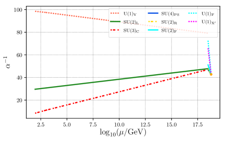
(a) Model 2: $n_{\mathrm{U_{V}}}=n_{\mathrm{E_{V}}}=1$.

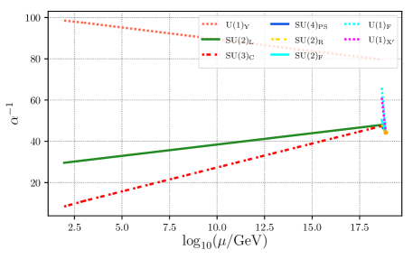
(b) Model 3: $n_{\mathrm{D_{V}}}=n_{\mathrm{E_{V}}}=1$.

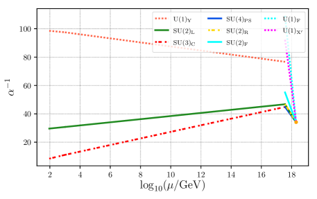
(c) Model 7: $n_{\mathrm{U_{V}}}=1,~{}n_{\mathrm{E_{V}}}=3$.

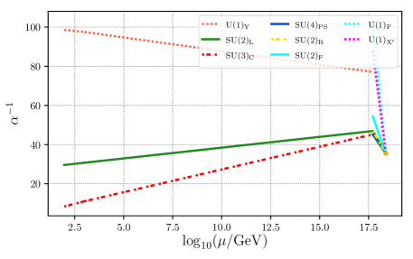
(d) Model 9: $n_{\mathrm{D_{V}}}=1,~{}n_{\mathrm{E_{V}}}=3$.

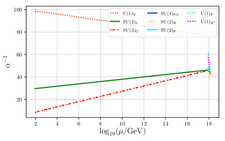
(e) Model 10: $n_{\mathrm{U_{V}}}=1,~{}n_{\mathrm{E_{V}}}=3,~{}n_{\mathrm{H}}=1$.

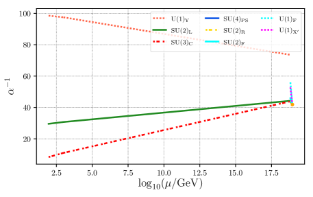
(f) Model 11: $n_{\mathrm{U_{V}}}=2,~{}n_{\mathrm{E_{V}}}=3,~{}n_{\mathrm{L_{V}}}=1$.

Figure 1: RG evolution of the gauge couplings in the non-minimal Pati-Salam GUT for six viable low-scale models compatible with exact unification of all interactions. In all cases shown above we have $\mu_{{}_{\mathrm{VLF}}}=1~{}\mathrm{TeV}$ as in Tab. 3. The orange dot represents the unification point with a universal gauge coupling $g_{8}$.

VI Conclusions

We have studied an anomaly-free realization of a non-minimal Pati-Salam GUT unified under the $\mathrm{E}_{8}$ symmetry. The 10-dimensional theory contains one vector $\bm{248}$ as well as five chiral $\bm{248}$-plets. The 4-dimensional limit of the $\mathrm{E}_{8}$ theory upon $\mathbb{Z}_{6}\times\mathbb{Z}_{2}$ orbifold compactification contains massless zero modes that can describe all SM gauge fields, chiral matter and right-handed neutrinos. We have shown that, in the limit of approximately degenerate superpotential mass parameters, our Pati-Salam GUT can naturally contain vector-like fermions at low-energy scales and at the reach of LHC or future collider experiments. In particular, the unification of the gauge couplings under $\mathrm{E}_{8}$ requires that such exotic fermions can either be $\mathrm{SU}(2)_{\mathrm{L}}$ singlet VLQs or both singlet and doublet VLLs. In total, we have found 13 viable models with New Physics manifest at $1~{}\mathrm{TeV}$ or at $10~{}\mathrm{TeV}$, making our model falsifiable at the LHC or future colliders.