Einstein on Involutions in Projective Geometry

Abstract

We discuss Einstein’s knowledge of projective geometry. We show that two pages of Einstein’s Scratch Notebook from around 1912 with geometrical sketches can directly be associated with similar sketches in manuscript pages dating from his Princeton years. By this correspondence, we show that the sketches are all related to a common theme, the discussion of involution in a projective geometry setting with particular emphasis on the infinite point. We offer a conjecture as to the probable purpose of these geometric considerations.

1 Introduction

Assessment of Einstein’s mathematical knowledge and proficiency is crucial for a historical understanding of his creativity as a physicist. The question of Einstein’s knowledge of mathematics has therefore been discussed frequently in the historical literature. Pyenson, (1980) already looked closer at Einstein’s mathematics education, concluding that he had an “excellent preparation for his future career” (p. 399). The publication of the first volume of Einstein’s Collected Papers in 1987 then provided the most important primary documents (Stachel,, 1987). Publication of the early correspondence between Einstein and Mileva Marić not only provided details about Einstein’s undergraduate studies in Zurich but also revealed the close communication between Einstein and his fellow student and later wife. The collaboration between the two gave rise to a much-debated issue of Mileva Marić’s role in their collaboration based on conjectures that she had provided the mathematics for Einstein’s discovery of special relativity (Troemel-Ploetz,, 1990; Stachel,, 1996). Cahan, (2000) and more recently Bracco, (2017) also look at Einstein’s early education but focus on his physics training. The question plays a role for an assessment of Einstein’s heuristics as well as the role of mathematics in Einstein’s physical theorizing (Zahar,, 1980), (Norton,, 2000). Studies of Einstein’s own calculations in the so-called Zurich Notebook from 1912 provided insights into his own learning process with respect to tensor calculus as well as into his way of putting mathematical concepts to use in his attempts to find a relativistic field theory of gravitation (Norton,, 1984; Renn and Sauer,, 1999; Janssen et al.,, 2007).

Einstein’s own published writings do discuss mathematical topics although rarely ever with explicit references to specialized literature. In his collaboration, he often relied on mathematicians to assist him in his physical theorizing. A well-known example is the 1913 Entwurf paper, presenting a precursor version of general relativity, which was co-authored with his mathematician friend Marcel Grossmann (Einstein and Grossmann,, 1913). The paper clearly declares their respective division of labor by the fact that Einstein authored its physical part and Grossmann its mathematical part. The final breakthrough to the fully covariant general theory, however, Einstein made on his own in late 1915 in competition with the mathematician David Hilbert.

In this paper, we intend to shed more light on Einstein’s mathematical knowledge, understanding and skills by looking at Einstein’s own research notes. We will discuss some specific arguments in projective geometry that Einstein is documented to have pondered in his deliberations.

In this project, we rely on the analysis of unpublished research notes and calculations, in particular his unpublished Princeton working sheets (Sauer,, 2019). It turns out that Einstein very rarely used graphical sketches or geometric constructions in his notes. This in itself is a noteworthy fact in light of his own statements about the non-verbal character of his thinking (Hadamard,, 1945, Appendix II). There is the occasional sketch of a coordinate system or reference frame. But in contrast to, for example, notes by his friend Grossmann, he rarely prepared any more elaborate geometrical constructions or the like. Instead, the vast majority of his private notes and calculations are algebraic in nature. We did identify, however, some pages in the Einstein Archives which document some rather specific arguments in the context of projective geometry. We will discuss these pages in some detail and claim that the very same argument was entertained by Einstein both in a research notebook dated to the years 1912–1915, and in research notes which we have dated to the summer of 1938.

The outline of our paper is as follows. In section 2, we recapitulate the basic facts about Einstein’s studies and his academic training in mathematics, establishing that he was probably well acquainted with basic concepts of projective geometry of the plane. In section 3, we then introduce our primary evidence, a double page in the Scratch Notebook of his Prague and Zurich years as well as a few manuscript pages from his Princeton working sheets. We will argue that these pages contain geometric constructions as well as analytical calculations that all pertain to the notion of projective involutions. A brief summary of our reconstruction of the double page of the notebook is given in section 4. In section 5, we discuss some relevant literature on projective geometry, both to the extent that Einstein may have been familiar with it and with respect to discussions of specific aspects of the reconstruction. In the following sections 6, 7, and 8, we will show in detail how very similar considerations are underlying a number of sketches found in the Princeton manuscripts. In section 6, we discuss involutions on a line, section 7 discusses involutions on a conic. We show how Einstein constructs geometric representations of involutions on a conic by starting from Pascal’s theorem and reducing the hexagon to a quadrangle. In section 8, we will give a reconstruction of a sketch and calculation in which Einstein gives both an analytical treatment and a graphical representation in terms of radical axis and involution by means of intersecting circles. We show that the corresponding consideration of the Scratch Notebook is a special case of the more general argument on the later manuscript page. For the sake of completeness, we mention and briefly discuss some further pertinent sketches in section 9, and section 10 serves as a caveat by pointing out some alternative scenarios of interpretation. In section 11, we finally address the question of the overall context of Einstein’s considerations of involution. We formulate a conjecture as to the probable purpose of Einstein’s considerations, We end in section 12 with some concluding remarks.

2 Einstein’s Studies in Projective Geometry

2.1 Early Studies in Munich, Milano, and Aarau

Einstein attended primary school and spent the first years of secondary school in Munich, first at a local Volksschule, then at the renowned Luitpold-Gymnasium. During those years, he also benefitted from private tutoring by the medical student Max Talmey who exposed him to a variety of advanced texts in all fields. In his autobiographical recollections, he recalled being fascinated by a magnetic compass and then continued:

At the age of 12 I experienced a second wonder […]: in a little book dealing with Euclidean plane geometry. (Einstein,, 1949, p. 9)

The book which he also called the “holy geometry booklet” (ibid., p. 11) most likely was the second part of Sickenberger’s (1888) Leitfaden der elementaren Mathematik, dealing with Planimetrie. On Talmey’s advice, he probably also studied Spieker’s (1890) Lehrbuch der ebenen Geometrie, see (Stachel,, 1987, p. lxi). One of his earliest known writings is a comment in the margin of Heis and Eschweiler, (1878), criticizing a proof that the cylinder can be developped into a plane (Stachel,, 1987, p. 3). He also remembered that he was studying mathematics eagerly as a teenager:

At the age of 12–16 I familiarized myself with the elements of mathematics together with the principles of differential and integral calculus. (Einstein,, 1949, p. 15)

After Einstein had left Munich, he spent a year with his family in Milano engaging in autodidactic studies in preparation for an entrance examination to be admitted as a student at the Zurich Polytechnic. Failing this examination, he was nonetheless encouraged and advised to finish his secondary schooling. Accordingly, he attended then the final class at Aargau cantonal school from October 1895 to September 1896. One of his teachers there was Heinrich Ganter who taught geometry following his own textbook. It was co-authored with Ferdinand Rudio, professor at the Polytechnic (Ganter and Rudio,, 1888), and treated plane geometry with an extensive discussion of conic sections. Einstein’s school record from the Aargau cantonal school indicates that he received the highest grades in algebra and geometry.

One of the questions for his Matura examinations in Aarau concerned the following problem of conic sections in plane Euclidean geometry:

Consider a circle of radius $r$, centered on the origin of a rectangular coordinate system. At each point along the $x$-axis, another circle is constructed, with center at this point and diameter determined by the intersections of the perpendicular to the $x$-axis with the original circle. The circles so constructed are enveloped by an ellipse of semiaxes $r$ and $r\sqrt{2}$. When the distance of the centers of the circles from the origin exceeds a certain maximum value, the circles cease to touch the envelope. Prove the last two statements and determine this maximum value. (Stachel,, 1987, Doc. 23, n. 5)

Figure 1: Illustration of a geometry problem presented to Einstein for his Matura examination.

For an illustration of this problem, see Fig. 1. In his solution, which did not involve any drawings, Einstein correctly derived the analytic expression for the enveloping ellipse and the distance $r/\sqrt{2}$ of the center from the center of the ellipse of the smallest osculating circle.

2.2 ETH 1896 and 1897

After graduating from Aargau cantonal school, Einstein took his undergraduate studies in Switzerland at Zurich’s Eidgenössische Polytechnische Schule (Federal Polytechnic School, in 1911 renamed to Eidgenössische Technische Hochschule (Swiss Federal Institute of Technology, ETH) from 1896 to 1900. He was one of eleven students initially enrolled in department VI A: the School for Mathematics and Science Teachers, section of mathematics, physics, and astronomy.

In his first year at the Polytechnic, Einstein took a class by Otto Wilhelm Fiedler on descriptive geometry, “Darstellende Geometrie”, and in the second year, in summer 1897 and winter 1897/98, he attended lectures on projective geometry, “Projektivische Geometrie I” and “Projektivische Geometrie II,” respectively, also held by Fiedler. In a letter to Mileva Marić, he wrote in 1898: “Fiedler lectures on projective geometry, he is the same indelicate, rude man as before & in addition sometimes opaque, but always witty & profound – in brief, a master but, unfortunately, also a terrible schoolmaster.” Fiedler’s (1871) textbook on descriptive geometry already included many elements of what later became projective elements, and its third edition (Fiedler,, 1883, 1885, 1888) had not only expanded to three volumes but its title programmatically expressed an “organic connection” between descriptive geometry (“Darstellende Geometrie”) and projective geometry (“Geometrie der Lage”).

As to the actual content of Fiedler’s lecture at the ETH in 1897, the first of these lecture courses is documented by a transcript, written by Marcel Grossmann, (1897). Grossmann was a good friend and classmate of Einstein and obtained his diploma together with Einstein in 1900. After this, he became assistant to Fiedler, obtained his Ph.D. in 1902 under Fiedler’s supervision and was from 1907 on his successor for “Descriptive Geometry” (“Darstellende Geometrie”) und “Projective Geometry” (“Geometrie der Lage”) (Graf-Grossmann,, 2015, 100–119). We know from Einstein’s recollections (Einstein,, 1955, 147) and a letter to Grossmann that he frequently borrowed Grossmann’s notes for test preparation, calling himself a “slovenly guy who wouldn’t even have been able to pass his examinations without the help of Grossmann’s notebooks.” In fact, in one of Grossmann’s lecture transcripts of infinitesimal geometry (Grossmann, 1898b, , 105), there is a note not made by Grossmann that can most probably be traced back to Einstein (Sauer,, 2015). It is safe to assume that Einstein carefully studied Grossmann’s lecture notes on Fiedler’s projective geometry, too.

Topics of the first lecture course in projective geometry of summer 1897 (Grossmann,, 1897) included, among others, the cross ratio of four distinct points, homogeneous coordinates, duality, conics, collineations, harmonic relations, and imaginary elements. Besides, Fiedler discussed involutions and Pascal’s theorem. As listed in his Record and Grade Transcript, Einstein received grades $4.5$ and $4$ (of $6$) in the two courses of projective geometry, respectively. Einstein’s grades result in a final grade of $4.25$ of his final transcript (“Abgangszeugnis”) which was his worst one. Marcel Grossmann received in the two courses of projective geometry grades of $5$ and $5.5$.

It should be noted that prior to axiomatic foundations of the field which, to be sure, were fully worked out at the latest with Veblen and Young, 1910a ; Veblen and Young, 1910b , projective geometry was not a clearly defined field, and many topics that today are seen as characteristically projective were discussed in the nineteenth and early twentieth century in other contexts as well, say, descriptive geometry. This is the case, in particular, with Fiedler’s understanding of geometry (Volkert,, 2020).

Thus, as a student of the Aargau cantonal school and the Zurich Polytechnic, Einstein was exposed to an education in mathematics and physics of high standards, including training in geometry in its various subdisciplines. He was a good student with excellent grades in mathematics and physics. His academic teacher Fiedler was instrumental in creating projective geometry as a field of academic study (Kitz,, 2015), and we know that Einstein studied Fiedler’s and other lectures, at least, through the carefully worked out notes prepared by his fellow student and friend Marcel Grossmann, who incidentally became Fielder’s successor at the ETH in 1907.

In order to assess to what extent Einstein retained an active command of the more sophisticated mathematical tools and concepts that he was exposed to during his studies, we need to turn to his later writings. By its very nature, a particularly revealing source are private research notes, in which he explored ideas for himself. Regarding projective geometry, we will here look at some of those manuscript pages.

3 Evidence: the Scratch Notebook and the Princeton Manuscripts

Among Einstein’s early research notes which are extant there is a Scratch Notebook with entries dated to the years 1910–1914. The double page of the Scratch Notebook that we will reconstruct in this article, is displayed in Fig. 2.

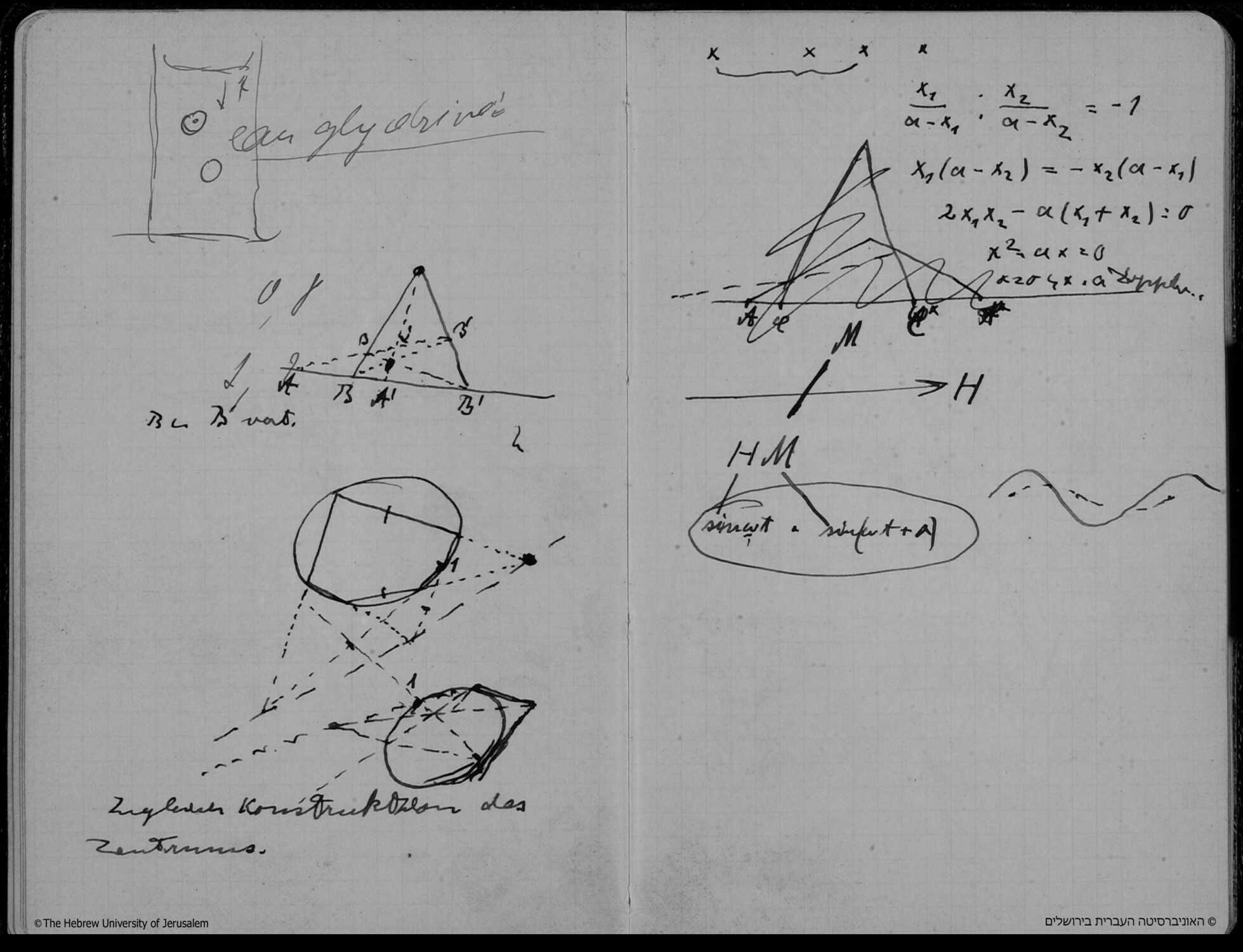
Figure 2: Double page in Einstein’s Scratch Notebook with sketches on projective geometry. AEA 3-013 [pp. 49–50], (Klein et al., 1993a, , p. 588). Reproduced with permission from the Albert Einstein Archives. ©The Hebrew University of Jerusalem, Israel. Digital image photographed by Ardon Bar Hama.

At the top of the left hand page, it displays a sketch drawn with pencil and the words “eau glyceriné” written in an unknown hand. In the middle of the right hand page, it shows sketches that carry letters $H$ and $M$ as well as the expression $\sin(\omega t)\cdot\sin(\omega t+\alpha)$. We conjecture that these entries are related to the discussion of problems related to Brownian motion and to magnetism, respectively. They may reflect conversations Einstein had with Jean Perrin and Paul Langevin, both of whom he met on a visit to Paris to give a lecture on the law of photochemical equivalence to the Societé de physique on 27 March 1913, see (Klein et al., 1993b, , Doc. 437). We will not be concerned with these entries on the double page but focus on the remaining entries.

The double page is preceded in the notebook by a sequence of pages that contain calculations on gravitational lensing, dated to spring 1912. It is immediately followed by a double page that also contains a calculation on gravitational lensing, which, however, was written at a later date, probably in late 1915. For a detailed discussion of the surrounding pages and calculations, see Sauer, (2008); Sauer and Schütz, (2019) and references therein.

Interpreting the four $x$’s with an underbrace at the top of the right hand page as an independent sketch, we therefore find five sketches on this double page—three on the left hand side and two on the right hand side—as well as five lines of calculations that are related to projective geometry. It is our aim to account for these entries.

Our reconstruction of the double page in the Scratch Notebook is based on a striking similarity that the sketches displayed there show with sketches that are found on three of Einstein’s Working Sheets from his Princeton years. The pages in question carry archival numbers AEA 62-785r, 62-787r, and 62-789 as well as 62-789r, see figure 3. All four manuscript pages can unambiguously be dated to the period between June and August 1938, since surrounding calculations and phrases directly link these pages to correspondence between Einstein and Peter Bergmann from that time about their paper on a Generalization of Kaluza’s Theory of Electricity (Einstein and Bergmann,, 1938) as well as a related Einstein manuscript. While the relative sequence of the three sheets is unclear, it is very likely that entries on the recto 62-789r precede entries on the verso 62-789.

The close connection between these sketches is in itself an intriguing fact. If the similarity were to result from Einstein’s entertaining the very same idea, it would be another instance of a long period of time between two characteristic trains of thought. Similarly, the surrounding lensing calculations of the Scratch Notebook from 1912–1915 were rediscovered, as it were, by Einstein in 1936 (Renn et al.,, 1997).

In addition to these pages, we will consider two more archival items that carry related sketches. One is an undated manuscript page AEA 124-446, likely from the early 1930’s. The other is AEA 6-250, a page from the Einstein-Bergmann correspondence, dated to the end of June 1938.

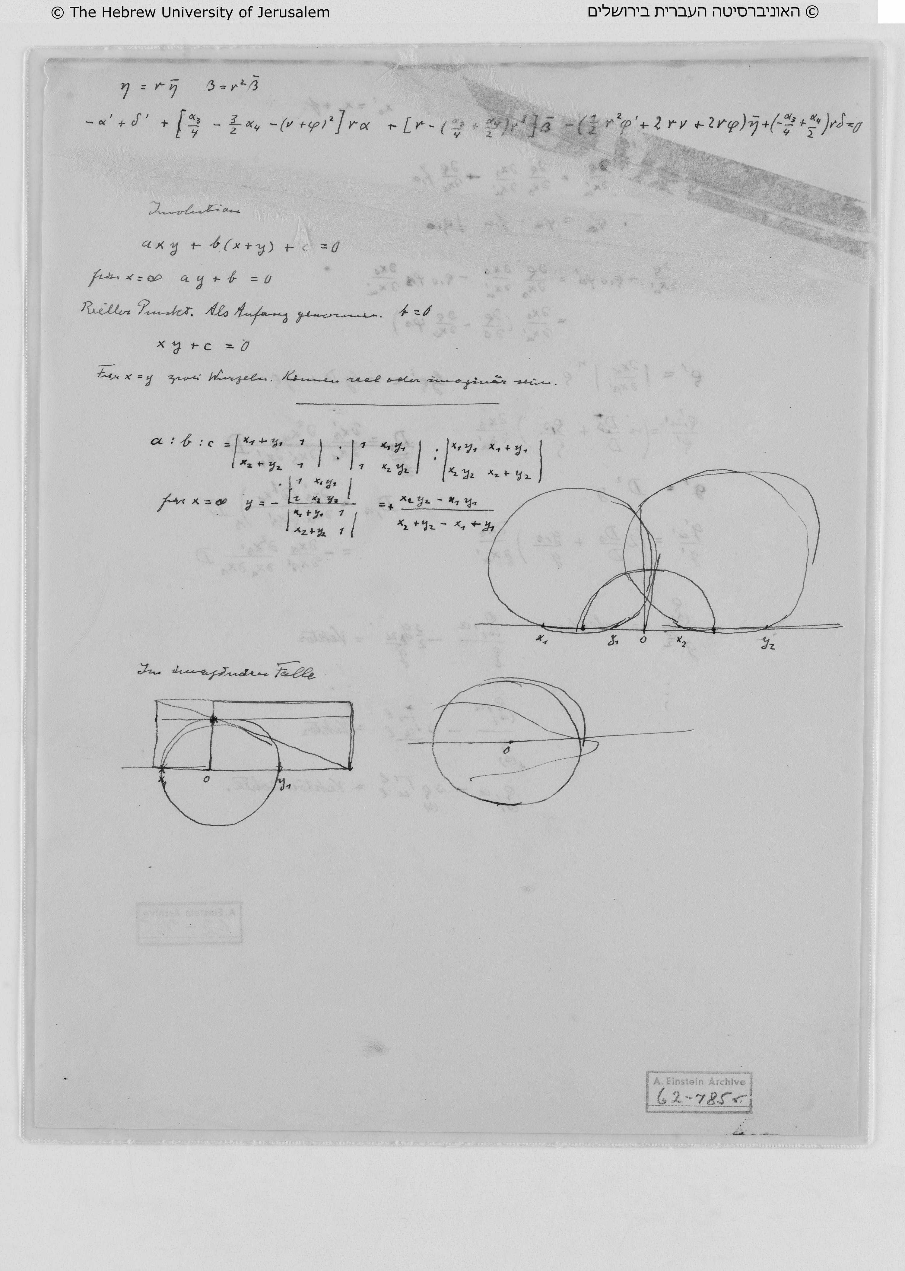
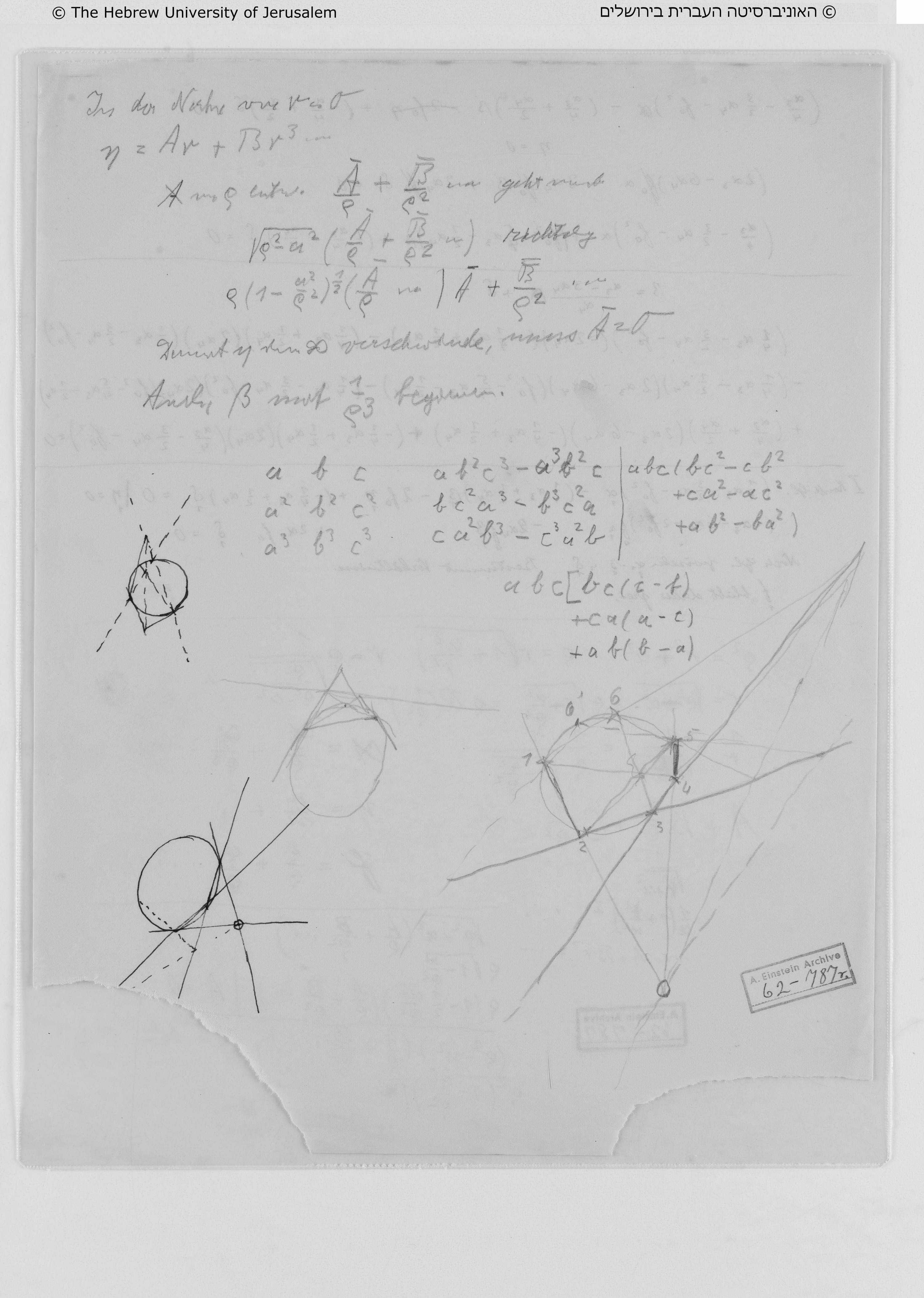
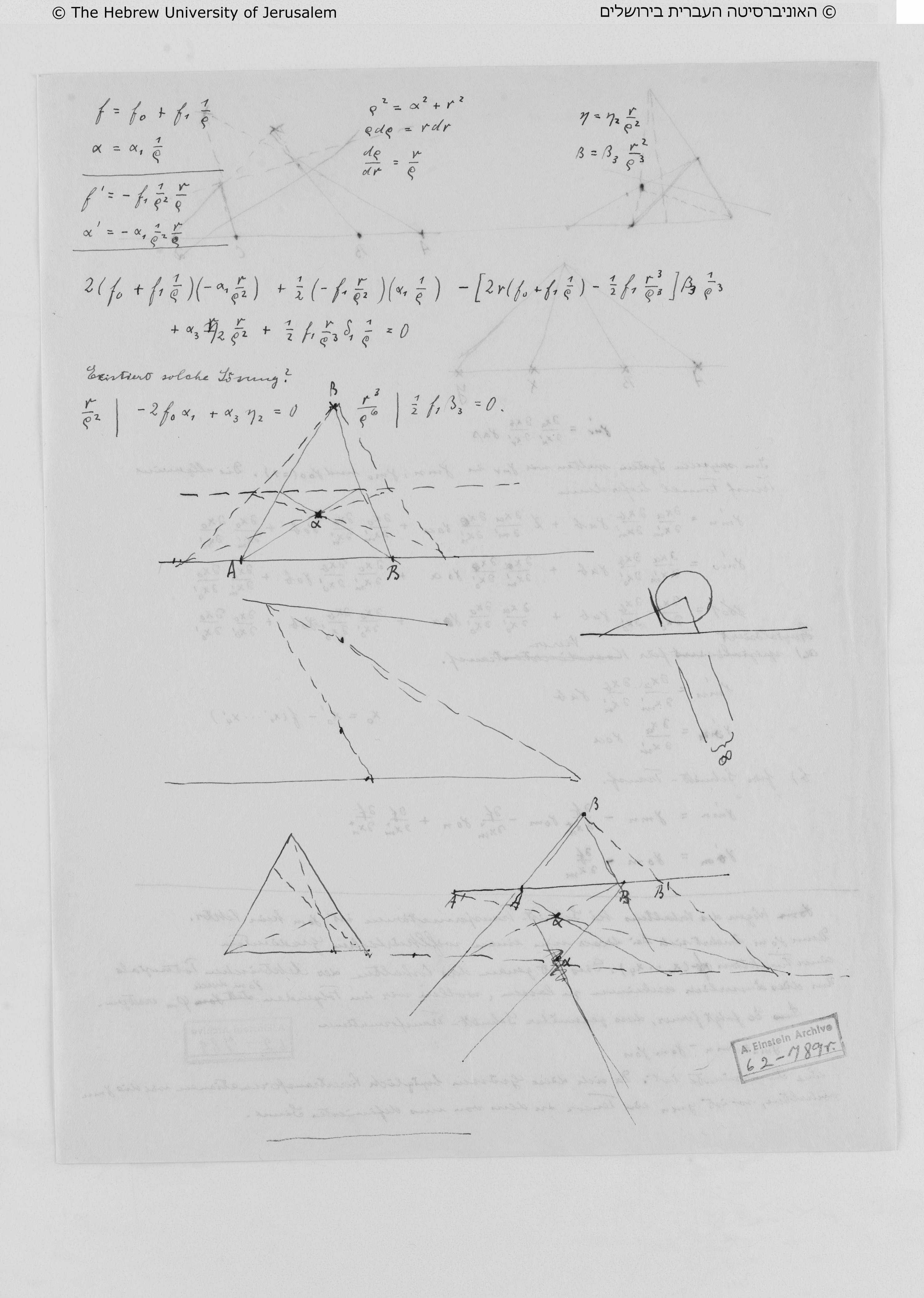
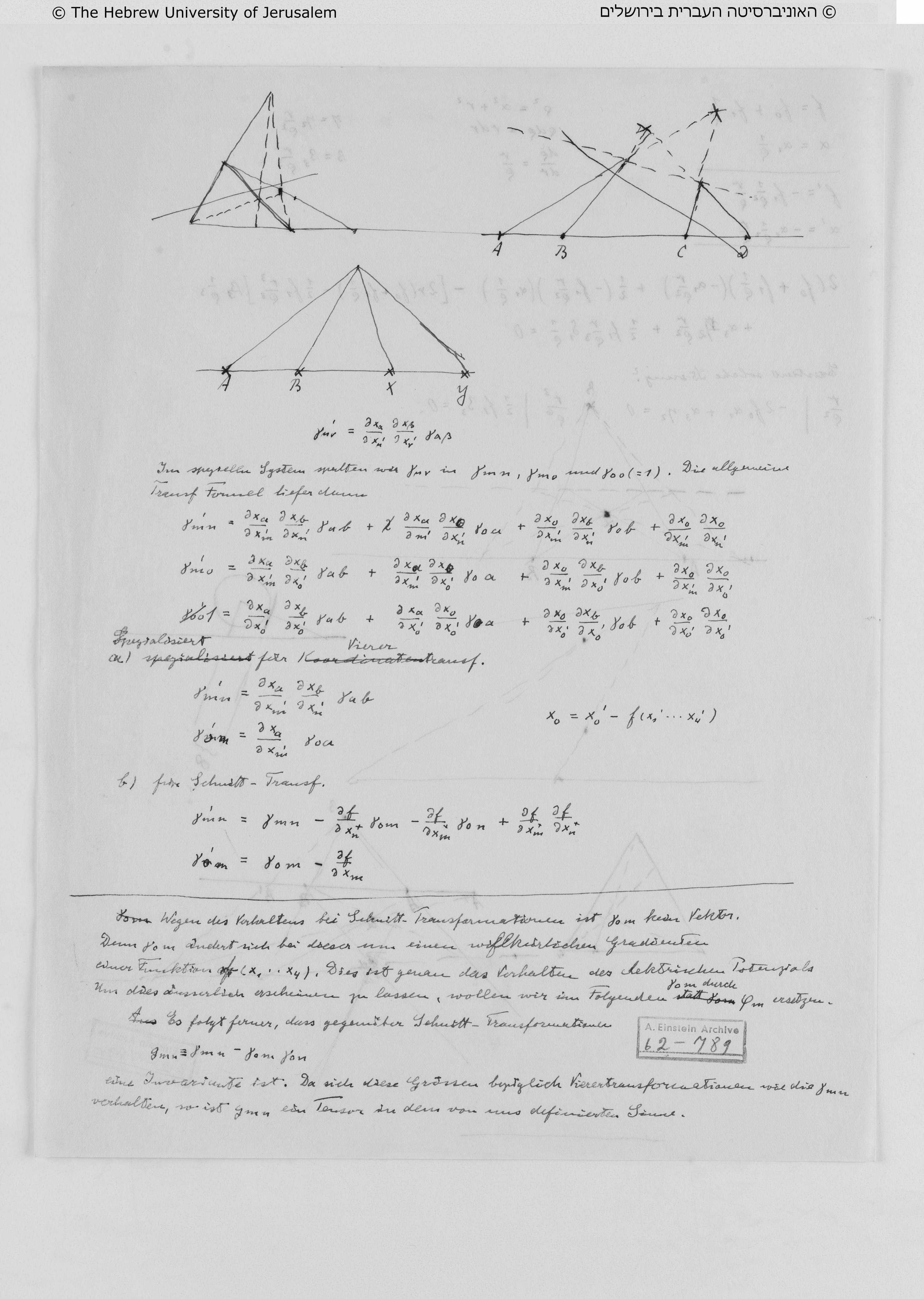
Figure 3: Manuscript pages AEA 62-785r, 62-787r, 62-789, 62-789r. Reproduced with permission from the Albert Einstein Archives. ©The Hebrew University of Jerusalem, Israel. Digital image photographed by Ardon Bar Hama.

4 Summary of our reconstruction

Despite the apparently disparate character of the entries on the double page, we will show that all five sketches as well as the five lines of calculations are related to each other as a cluster of considerations revolving around the notion of involution in a projective geometry setting. In summary, our reconstruction of the page is the following.

In the first sketch, Einstein constructs an example of a hyperbolic involution on a line by means of two consecutive perspectivities. The involution interchanges points $B$ and $B^{\prime}$ while points $A$ and $A^{\prime}$ are the two uniquely determined fixed points. In similar sketches from the Princeton manuscripts, he also investigated the case where one of the points of the involution moves to infinity.

The next sketch shows a construction of Pascal’s theorem for a hexagon inscribed in a conic. The purpose of this construction appears to be to provide a basis for the geometric construction of an involution in a conic by means of an inscribed quadrangle. He obtains the third sketch on the page by letting two pairs of adjacent points of the hexagon approach each other, so that the hexagon becomes a quadrangle. The respective secants of the conic are marked and become tangents after this transformation. In order to arrive at a hyperbolic involution, he also moves the point marked 1 along the conic across the tangent point. The procedure amounts to the geometric construction of a hyperbolic involution in the conic. The very same procedure of starting from an inscribed hexagon to an inscribed quadrangle is found with more explicit notation on manuscript page 62-787r. In addition to the case of a hyperbolic involution, Einstein there also draws two additional situations which represent the cases of elliptic and parabolic involution. On that page, he also considers the special case where two of the opposite sides of the inscribed hexagon for Pascal’s theorem become parallel. The Pascal line then becomes parallel to the sides and one of the three points on the Pascal line moves to infinity.

At the top of the next page, Einstein again considers involution on a line. He draws four collinear points and marks two of them which we interpret as indicating the two invariant points. Underneath we find a sketch that he deleted which we, again, interpret as a construction of hyperbolic involution on a line, this time, however, by means of a complete quadrangle.

The remaining entries to be accounted for are five lines of calculation. We interpret these as a special case of the general equation of involution for coordinates $x_{1}$ and $x_{2}$, which are then postulated to be invariant points of the involution, yielding two solutions $x=0$ and $x=a$. A corresponding and much more explicit calculation along these lines is found on manuscript page 62-785r. That calculation was explicitly headed by the term “Involution.” It starts from the general equation of involution and specifies to the case of one infinite point. In addition, the calculation on the manuscript page is accompanied by several sketches that give geometric constructions of the corresponding involution by means of the concept of a radical axis. Here again all three cases of hyperbolic, elliptic and parabolic involution are being considered.

Our reconstruction heavily depends on the similarity of the corresponding entries in the Princeton manuscript pages and the translatability between the notebook entries and the Princeton manuscript pages. In sections 6, 7, and 8, we will provide a detailed reconstruction of these connections. They are also visualized by some animations which illustrate the processes of construction and transformation that are involved in the reconstruction. These animations are provided as supplementary material to this article.

5 Projective Geometry

Before entering into our detailed reconstruction, we briefly mention some of the available textbook literature on projective geometry, both by texts that were available to Einstein as well as more modern treatises. We have not been able to identify any single work which might have triggered, or would have been an obvious source for, Einstein’s sketches. None of the geometric theorems and properties that underlie Einstein’s sketches are particularly specific to any single author, let alone original to Einstein. As a consequence similar sketches can be found in many places in the literature.

Beginning with sources that would have been available to Einstein prior to 1938, we mention again Fiedler’s textbook on Descriptive Geometry (Fiedler,, 1871) or (Fiedler,, 1883, 1885, 1888) and his Lectures, as well as Grossmann’s Lectures. As noted before, from an axiomatic standpoint, the field was presented by Veblen and Young, 1910a ; Veblen and Young, 1910b . As to more specific discussions, that might have been directly relevant, we note that Pascal’s theorem and especially its different versions are discussed by (Grassmann,, 1909, 95-101). His visualizations of the different versions look very similar to Einstein’s sketches on AEA 62-787r and in the Scratch Notebook. Enriques, (1915) is noteworthy for its statements about the radical axis and involutions on a line (Enriques,, 1915, 124-128). Discussion with sketches similar to Einstein’s sketches can also be found in older books from the beginning of the 20th century by, for example, Emch, (1905, 13–14), Hatton, (1913, 101), Askwith, (1917, 82), or Dowling, (1917, 131).

In our reconstruction of Einstein’s geometric arguments, we will often refer to Coxeter’s books on The Real Projective Plane from 1949 and on Projective Geometry from 1964. But, again, the subject matter is treated in many different ways in many different texts.

Finally, we would like to point out that in a little book which treats “the most famous problems of mathematics”, we found many theorems with visualizations vaguely reminiscent of Einstein’s sketches (Dörrie,, 1958, 261–284). Although the book is from 1958, the first edition was published in 1932. This book may be of interest because of Einstein’s predilection for amusing problems in mathematics as addressed in “Mathematische Mußestunden” by Hermann Schubert, (1898), some of which are found already in the Scratch Notebook, see also Rowe, (2011).

6 Involution on a line

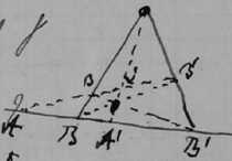
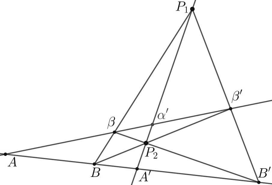
Figure 4: Hyperbolic involution with invariant points $A$ and $A^{\prime}$ that interchanges points $B$ and $B^{\prime}$. (a) Einstein’s first sketch in the Scratch Notebook. Reproduced with permission from the Albert Einstein Archives. ©The Hebrew University of Jerusalem, Israel. Digital image photographed by Ardon Bar Hama. (b) Reconstruction of Einstein’s sketch.

The sketches in figure 4 can be interpreted as a hyperbolic involution on a line that interchanges points $B$ and $B^{\prime}$, while points $A$ and $A^{\prime}$ remain invariant. Indeed, by (Coxeter,, 1987, 47), two invariant points $A$ and $A^{\prime}$ of an involution are harmonic conjugates with respect to any other pair of the involution. This holds in figure 4 by the construction of the complete quadrangle (Coxeter,, 1987, 22).

Einstein’s notation supports this interpretation. He apparently described the involution by the product of two perspectivities. Let us therefore note that Einstein marked points $P_{1}$ and $P_{2}$ each by a thick dot. Considering the perspectivity with center $P_{1}$, point $B$ goes to $\beta$, $A^{\prime}$ goes to $\alpha^{\prime}$, and $B^{\prime}$ goes to $\beta^{\prime}$, while the point $A$ remains invariant. Carrying out the second perspectivity with center $P_{2}$ takes $\beta$ to $B^{\prime}$, $\alpha^{\prime}$ back to $A^{\prime}$, and $\beta^{\prime}$ to $B$, while $A$ again remains invariant. The product of the two perspectivities, thus, interchanges the points $B$ and $B^{\prime}$ and lets the points $A$ and $A^{\prime}$ invariant. Einstein concluded: “$B$ and $B^{\prime}$ interchanged”, which he wrote directly underneath the sketch.

6.1 Transition to Manuscript Page AEA 124-446

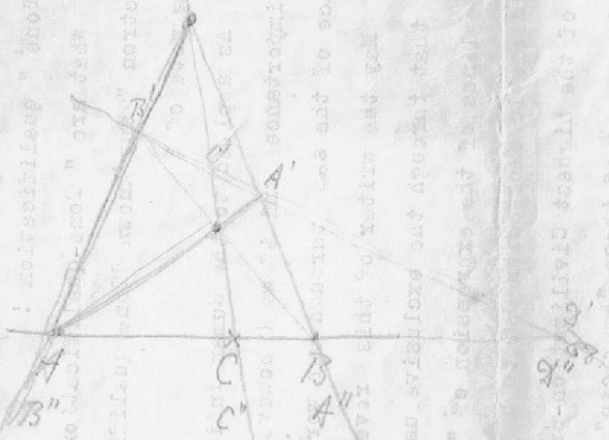
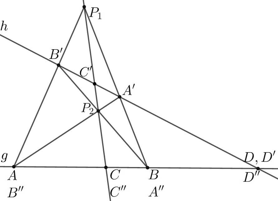
Figure 5: Involution with invariant points $C$ and $D$ that interchanges points $A$ and $B$. (a) Einstein’s second sketch on manuscript page AEA 124-446. Reproduced with permission from the Albert Einstein Archives. ©The Hebrew University of Jerusalem, Israel. Digital image photographed by Ardon Bar Hama. (b) Reconstruction of Einstein’s sketch.

Before discussing related sketches in the Princeton manuscripts, we observe that a sketch very similar to the first sketch in the Scratch Notebook can also be found on manuscript page AEA 124-446, see figure 5. To show the relation between the two sketches, we start from figure 4, move point $\beta$ up such that point $A$ vanishes at infinity and reappears to meet the base line $g$ on the right hand side of the complete quadrangle. Changing the notation, i.e. $B\rightarrow A$, etc., leads us to figure 5. Einstein’s notation suggests that in contrast to figure 4 he now carried out the perspectivity with center $P_{2}$ before the perspectivity with center $P_{1}$. By the first perspectivity, the point $A$ goes to $A^{\prime}$, $C$ goes to $C^{\prime}$, $B$ goes to $B^{\prime}$ and $D$ remains invariant while Einstein wrote down $D^{\prime}$ anyhow. By the second perspectivity with center $P_{1}$, $A^{\prime}$ goes to $B$ which is also denoted by $A^{\prime\prime}$, $B^{\prime}$ goes to $A$ which is also denoted by $B^{\prime\prime}$, $C^{\prime}$ goes back to $C$ which is also denoted by $C^{\prime\prime}$, and $D^{\prime}$ remains invariant which is also denoted by $D^{\prime\prime}$. The product of the two perspectivities thus interchanges the points $A$ and $B$, while the two points $C$ and $D$ remain invariant, in full equivalence to the situation in the Scratch Notebook. The notation here is even more directly indicating the procedure described above.

6.2 Similar Sketches on Manuscript Pages AEA 62-789 and 62-789r

Two similar sketches appear on manuscript page AEA 62-789 as well as on its reverse side AEA 62-789r, see figure 6.

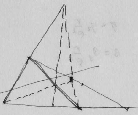
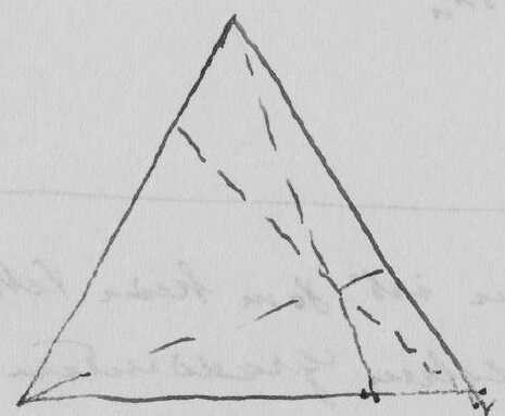
Figure 6: Sketches similar to the first sketch in the Scratch Notebook on manuscript pages AEA 62-789 and its reverse side 62-789r. (a) Einstein’s first sketch on manuscript page AEA 62-789. It is crossed out; (b) Einstein’s fourth sketch on manuscript page AEA 62-789r. Reproduced with permission from the Albert Einstein Archives. ©The Hebrew University of Jerusalem, Israel. Digital image photographed by Ardon Bar Hama.

However, Einstein here did not letter any points or lines and it is not as clear as before whether Einstein drew these sketches in the context of hyperbolic involutions. Indeed, both figures are very generic sketches in projective geometry, which allow for many different contexts as, for example, the discussion of the complete quadrangle and the harmonic relation of four points on a line, see (Coxeter,, 1987, 22). We will discuss another context in section 6.3, namely the construction of two invariant points and one pair of an involution.

The very same manuscript pages 62-789 and 62-789r, however, also show sketches that, again, can be related to the figures of the Scratch Notebook, see figure 7. Assuming the situation and notation of figure 5, we can ask what happens when line $h$ is turned around a bit to become parallel to the base line $g$. Einstein apparently investigated this situation in the first and fifth sketch on AEA 62-789r (figure 7). In this case, the fourth harmonic point $D$ goes to the point at infinity. Since the harmonic relation between the points $A$, $C$, $B$, and $D$ still holds, the point $C$ becomes the midpoint of the segment $AB$, see (Coxeter,, 1961, 119) or (Kaplansky,, 1969, 109). Einstein drew this situation in figure 7(a), where the points $A$ and $B$ are the same as in figure 5 and the line connecting $P_{1}$ and $P_{2}$ yielding the point $C$ is missing.

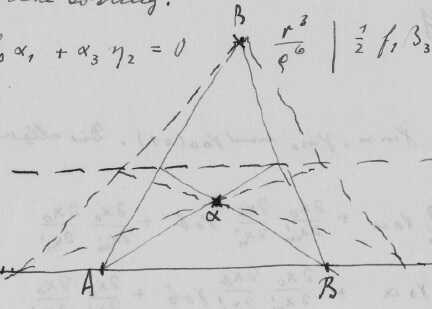
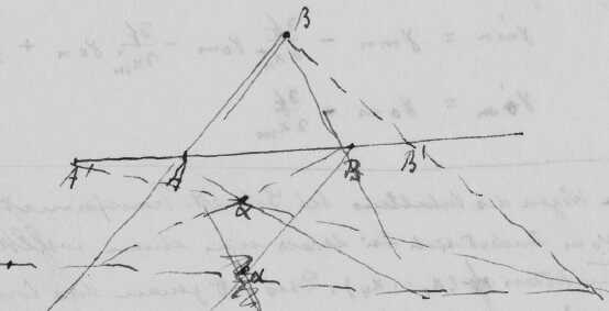
Figure 7: Sketches on AEA 62-789, where the fourth harmonic point meets line $g$ in the point at infinity. (a) Einstein’s first sketch on manuscript page AEA 62-789r; (b) Einstein’s fifth sketch on manuscript page AEA 62-789r. Reproduced with permission from the Albert Einstein Archives. ©The Hebrew University of Jerusalem, Israel. Digital image photographed by Ardon Bar Hama.

Einstein not only drew this situation for the points $A$ and $B$, but also for two points lying further out (see the dashed lines). In figure 7(b), he moved the dashed horizontal line underneath the solid horizontal line such that $\alpha$ now lies underneath $A$ and $B$. In this situation, he marked the two additional points lying further out by $A^{\prime}$ and $B^{\prime}$.

In addition to figures 6 and 7, the page contains two more sketches probably written in the context of projective geometry, although we have found no convincing reconstruction for them. One of these sketches has striking similarities to a sketch appearing in Grossmann’s lecture notes on “Projektivische Geometrie: Geometrie der Lage” held by Fiedler (Grossmann,, 1897, 41).

6.3 Another Sketch in the Scratch Notebook

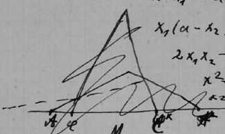
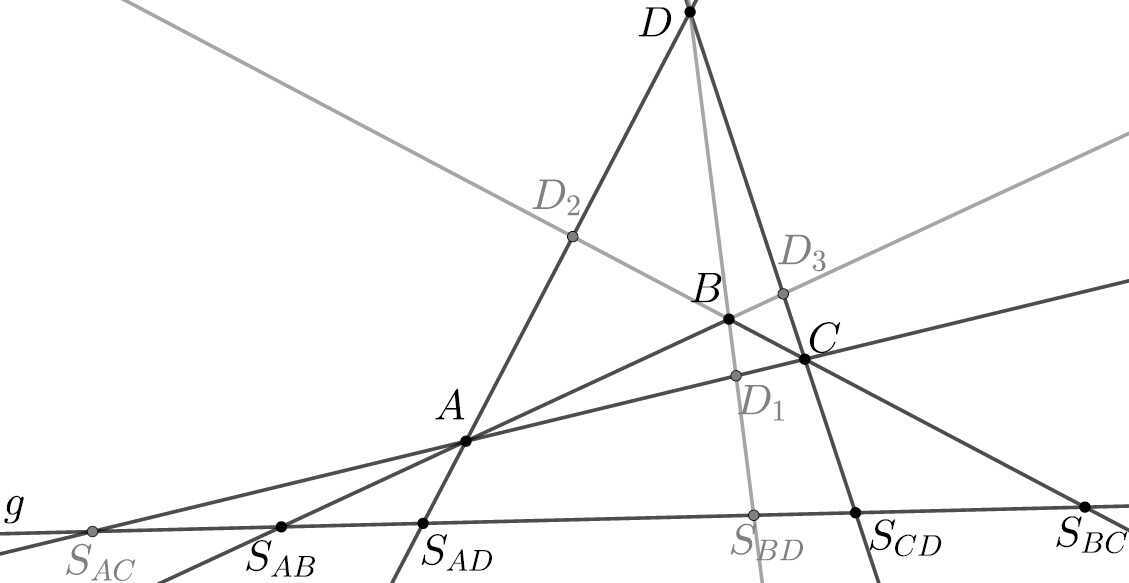
Figure 8: The construction of an involution on a line. (a) Einstein’s fifth sketch in the Scratch Notebook. It is crossed out. Reproduced with permission from the Albert Einstein Archives. ©The Hebrew University of Jerusalem, Israel. Digital image photographed by Ardon Bar Hama. (b) Reconstruction of Einstein’s sketch. He did not draw the gray objects.

Let us return to the Scratch Notebook. Einstein’s fifth sketch in the Scratch Notebook is shown in figure 8(a). We will use the notation of our reconstruction in figure 8(b). Considering the complete quadrangle with vertices $A$, $B$, $C$, $D$ and diagonal points $D_{1}$, $D_{2}$, $D_{3}$, opposite sides of the quadrangle meet a line $g$ in pairs of an involution, see Enriques, (1915, 122,123) or Dörrie, (1958, 269). This implies that $S_{AB}$ and $S_{CD}$ is a pair of the involution. Einstein denoted them by $A$ and $A^{\ast}$ but overwrote the notation of the second point afterwards. Another pair of the involution are the points $S_{AD}$ and $S_{BC}$, which were denoted as $C$ and $C^{\ast}$ by Einstein. The second point was then overwritten as well. The third pair $S_{AC}$ and $S_{BD}$ was not marked by Einstein. Since Einstein drew the line through $A$ and $C$, the intersection $S_{AC}$ is indicated, while he did not draw the line through $D$ and $B$, which would give the intersection $S_{BD}$. Note that Einstein in his sketch did not use the letter $B$, but did use $A$ and $C$.

It is neither clear why Einstein changed the notation of the two points on the right nor why he crossed out the entire sketch. The initial notation, however, suggests that he again considered the construction of an involution on a line.

By these considerations, we can get an alternative interpretation of figure 4. Let us consider the complete quadrangle with vertices $\beta$, $P_{1}$, $\beta^{\prime}$, $P_{2}$ and diagonal points $\alpha^{\prime}$, $B$, and $B^{\prime}$. In contrast to the situation of figure 8, the line $g$ then passes through two diagonal points $B$ and $B^{\prime}$, which is why we can interpret this sketch as the construction of an involution on the line $g$ with the pair $A$ and $A^{\prime}$ and the invariant points $B$ and $B^{\prime}$. This interpretation does not explain Einstein’s comment that the points $B$ and $B^{\prime}$ are interchanged nor does it explain the notation chosen by Einstein nor why he bolded points $P_{1}$ and $P_{2}$. However, it is possible that Einstein considered it this way in the process of drawing figure 8(a). By moving the point $P_{2}$ in figure 4(b) slightly to the upper right, we get figure 8. As we will see in the next section, it stands to reason that Einstein considered such a transition on the manuscript page AEA 62-789 as well.

6.4 Similarities to Manuscript Page AEA 62-789

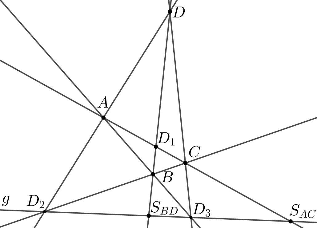
Figure 9: The first sketch on manuscript page AEA 62-789, interpreted as the construction of a pair and two invariant points of an involution on a line. (a) Einstein’s first sketch on manuscript page AEA 62-789. It is crossed out. Reproduced with permission from the Albert Einstein Archives. ©The Hebrew University of Jerusalem, Israel. Digital image photographed by Ardon Bar Hama. (b) Reconstruction of Einstein’s sketch.

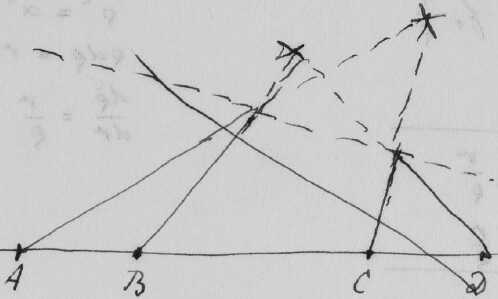
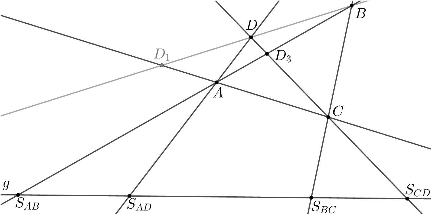
Figure 10: The second sketch on manuscript page AEA 62-789, interpreted as the construction two pairs of an involution on a line, see also figure 8. (a) Einstein’s second sketch on manuscript page AEA 62-789. It is crossed out. Reproduced with permission from the Albert Einstein Archives. ©The Hebrew University of Jerusalem, Israel. Digital image photographed by Ardon Bar Hama. (b) Reconstruction of Einstein’s sketch. He did not draw the gray lines.

If we turn over page 62-789r to look at 62-789, we find two sketches next to each other at the top of manuscript page. These again can be connected to the sketches in figures 4(a) and 8(a) in the Scratch Notebook. They are shown in figures 10 and 9.

By introducing notation as in figure 9(b) and considering the complete quadrangle with vertices $A$, $B$, $C$, $D$ and diagonal points $D_{1}$, $D_{2}$, $D_{3}$, the points $D_{2}$ and $D_{3}$ can be interpreted as invariant points of an involution on the line $g$, while points $S_{BD}$ and $S_{AC}$ are corresponding points.

If we move the point $B$ to the upper right, we directly get figure 10, where the line $g$ does not pass through any diagonal point anymore. Thus, the points $S_{AB}$, $S_{CD}$ and $S_{AD}$, $S_{BC}$ are corresponding points, respectively. Equivalently to figure 8, Einstein drew one more line whose intersection with $g$ determines one point of the third pair (line $AC$).

We conclude that all sketches from figures 4–10 can be interpreted in some way or other as constructions involving involutions on a line.

We also note that just as we find figures 4(a) and 8(a) next to each other on a double page of the Scratch Notebook, two very similar sketches appear right next to each other at the top of manuscript page AEA 62-789.

7 Pascal’s Theorem and Involution on a Conic

Surprisingly, we find a similar correspondence between sketches in the Scratch Notebook and manuscript page 62-787. These sketches deal with projective geometry on conics.

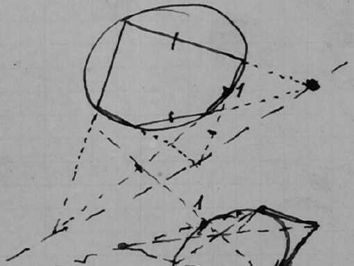
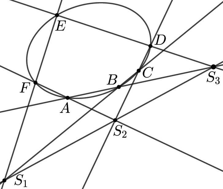
Figure 11: Pascal’s theorem. Opposite sides of a hexagon inscribed in a conic meet in three collinear points. (a) Einstein’s second sketch in the Scratch Notebook. Reproduced with permission from the Albert Einstein Archives. ©The Hebrew University of Jerusalem, Israel. Digital image photographed by Ardon Bar Hama. (b) Reconstruction of Einstein’s sketch.

Einstein’s Scratch Notebook shows a second sketch, which is shown in figure 11 together with our reconstruction. As the only numbered point he denoted point $C$ by $1$. He also drew point $S_{3}$ as a thick dot and marked lines $ED$ and $AB$. The sketch visualizes Pascal’s theorem which states that opposite sides of a hexagon $ABCDEF$ inscribed in a conic meet each other in three collinear points $S_{1}$, $S_{2}$, and $S_{3}$ (Coxeter,, 1961, 103). The line passing through these points is called Pascal line.

The sketch just underneath shows a quadrangle inscribed in a conic, see figure 12. Again, by our reconstruction, point $C$ was numbered $1$ by Einstein. By (Grassmann,, 1909, 99), in this situation the tangents in $A$ and $D$ as well as the opposite sides $AF$, $DC$ and $AC$, $DF$ meet each other in three collinear points $S_{1}$, $S_{2}$, $S_{3}$.

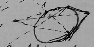
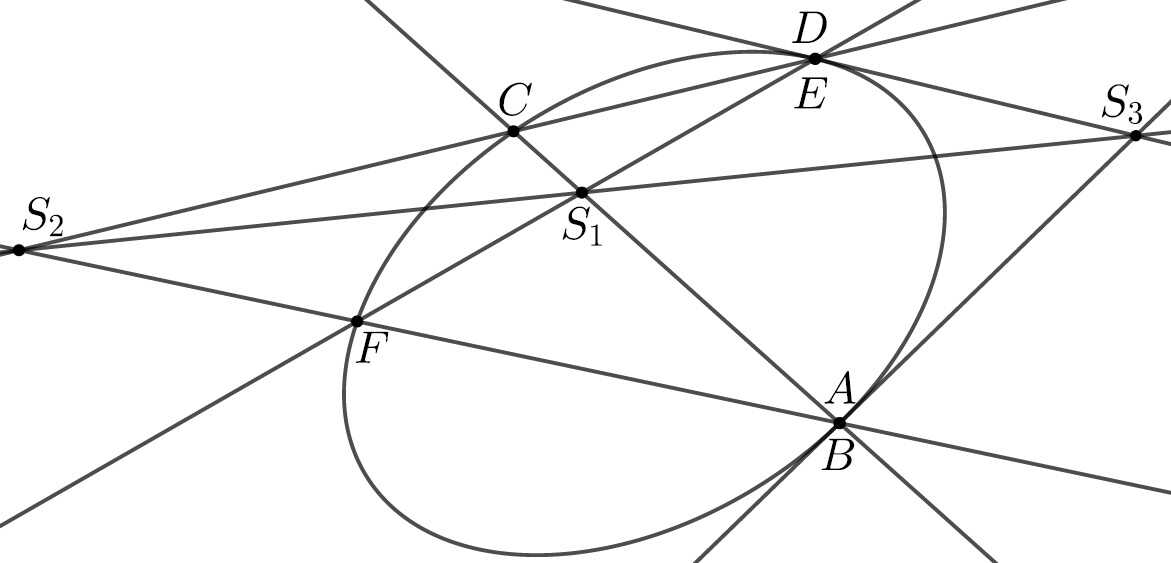
Figure 12: Pascal’s theorem for a quadrangle. (a) Einstein’s third sketch in the Scratch Notebook. Reproduced with permission from the Albert Einstein Archives. ©The Hebrew University of Jerusalem, Israel. Digital image photographed by Ardon Bar Hama. (b) Reconstruction of Einstein’s third sketch in the Scratch Notebook.

Steiner’s theorem enables us to define projectivities on conics (Coxeter,, 1961, 105), which again allows us to interpret Einstein’s sketches as investigations of projectivities and involutions. Figure 11(b) can be interpreted as the projectivity $AEC\barwedge DBF$. In this particular case, the Pascal line becomes the axis of the projectivity.

When moving toward each other points $A$ and $B$ as well as $E$ and $D$, respectively, the secants $AB$ and $ED$ in figure 11 become tangents which meet in $S_{3}$. This procedure was indicated by Einstein by marking these two lines as well as point $S_{3}$. When furthermore moving point $C$ along the conic such that it comes to lie between points $F$ and $E=D$, we obtain Einstein’s sketch in figure 12. Moving point $C$ into this position was also indicated by Einstein since it is the only point numbered in both figure 11(a) and figure 12(a).

The projectivity $AEC\barwedge DBF$ from figure 11 then becomes $ADC\barwedge DAF$. This means that the projectivity interchanges points $A$ and $D$ and thus is an involution (Coxeter,, 1987, 45). By knowing another pair $C$, $F$ of the involution, it is fully determined (Coxeter,, 1987, 45). As we see in figure 12, the Pascal line furthermore crosses the conic in two points which are the invariant points of the involution, which therefore is a hyperbolic one.

Beneath the third sketch, Einstein wrote: “At the same time construction of the center.” Any secant through the center of the involution determines a pair of the involution as the two intersections with the conic (Coxeter,, 1961, 108-109). Since figure 12 can be interpreted as the involution $ADC\barwedge DAF$, the intersection of the lines $AD$ and $CF$ determines the center of the involution. This might be the idea of Einstein’s additional comment, since he did not draw these lines.

7.1 Similarities to Manuscript Page AEA 62-787r

The manuscript page AEA 62-787r contains sketches that are astonishingly similar to the second and third sketch in the Scratch Notebook that we have just discussed. Moreover, this page illustrates the ideas from the previous section by a more precise notation as well as by additional sketches.

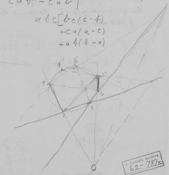
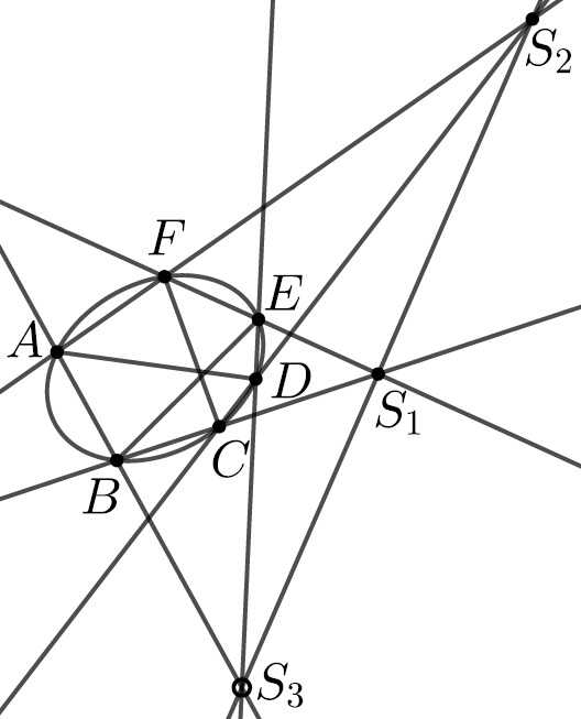
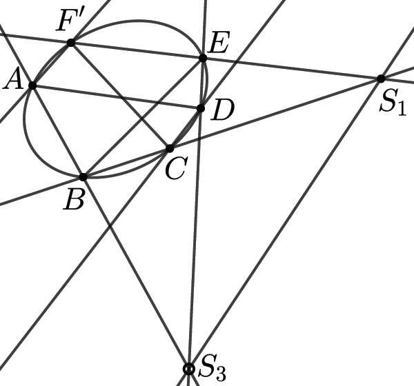
Figure 13: Pascal’s theorem. (a) Einstein’s sketch on the right hand side of manuscript page AEA 62-787r. Reproduced with permission from the Albert Einstein Archives. ©The Hebrew University of Jerusalem, Israel. Digital image photographed by Ardon Bar Hama. (b) Reconstruction of Einstein’s sketch ignoring point $6^{\prime}$; (c) Reconstruction of Einstein’s sketch ignoring point $6$.

Let us start with the sketch on the right hand side of the manuscript page, see figure 13(a). It shows Pascal’s theorem, just as in figure 11, but Einstein here combined two different situation into this sketch. The first situation is shown in figure 13(b). Einstein numbered points on the conic from $1$ to $6$, while we denoted them by $A$ to $F$. The sketch therefore is an identical repeat of illustrating Pascal’s theorem as in figure 11. Einstein then replaced point $F$ by $F^{\prime}$ such that the opposite lines $AF^{\prime}$ and $CD$ become parallel. They then meet in the point at infinity $S_{2}$. By Pascal’s theorem, the Pascal line which connects $S_{1}$ and $S_{3}$ needs to pass through the point at infinity $S_{2}$ as well, which is why it becomes parallel to these opposite sides.

By these considerations, we can explain most of the lines drawn by Einstein. However, Einstein also drew the line segments $AD$, $BE$, and $CF$ inside the conic. These segments indicate that Einstein considered the projectivity $AEC\barwedge DBF$. In this case, he connected the corresponding points by a line segment. Considering this projectivity, the axis of the projectivity becomes the Pascal line, which is drawn by Einstein.

As in the Scratch Notebook, Einstein marked the point $S_{3}$. Moreover, he also bolded lines $ED$ and $AB$. In order to get figure 13(b) starting from figure 11(b), we only need to move some points along the conic without the need of changing the orientation.

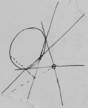
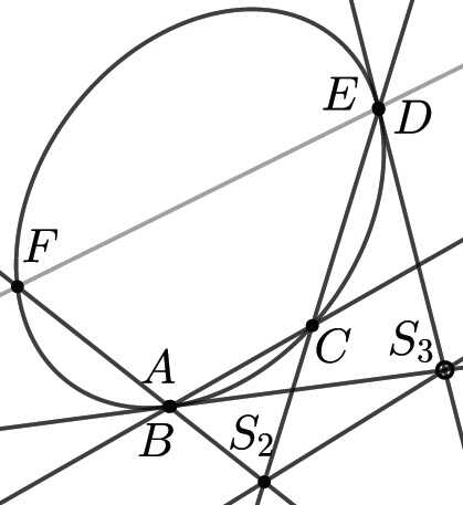
Figure 14: Elliptic involution on a conic. (a) Einstein’s sketch in the bottom left corner of manuscript page AEA 62-787r, which was not drawn accurately. Reproduced with permission from the Albert Einstein Archives. ©The Hebrew University of Jerusalem, Israel. Digital image photographed by Ardon Bar Hama. (b) Reconstruction of Einstein’s sketch. He did not draw the gray line $EF$.

As in the discussion of the second and third sketch in the Scratch Notebook, we can now let the points $A$, $B$ and $E$, $D$ approach each other. These two lines then become tangents meeting in the marked point $S_{3}$. By slightly rearranging the points on the conic, we then get the situation in figure 14, which is another sketch on manuscript page 62-787r. We see that Einstein also marked point $S_{3}$ in this sketch indicating the transition just described.

In contrast to the discussion of the Scratch Notebook (figures 11 and 12), we have not moved point $C$ yet. As a result, we do not get a hyperbolic involution, but an elliptic involution $ADC\barwedge DAF$. The Pascal line that goes through $S_{2}$ and $S_{3}$ is an exterior line without intersections with the conic such that no invariant point exists. We note that Einstein’s sketch is not accurate as the intersection $S_{1}$ of $EF$ and $BC$ would meet on the right side of the conic in Einstein’s sketch, while the Pascal line meets the line $BC$ rather on the left side of the conic (the piece that had been torn off).

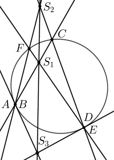
Figure 15: Hyperbolic involution on a conic. (a) Einstein’s top left sketch on manuscript page AEA 62-787r. Reproduced with permission from the Albert Einstein Archives. ©The Hebrew University of Jerusalem, Israel. Digital image photographed by Ardon Bar Hama. (b) Reconstruction of Einstein’s sketch.

We can now proceed by moving point $C$ such that it comes to lie between $E=D$ and $F$. By changing the orientation, we then get the situation in figure 15, also found on 62-787r. This sketch can be interpreted as a hyperbolic involution $ADC\barwedge DAF$, since the Pascal line intersects the conic in two points. We only need to rotate this sketch by $90^{\rm o}$ in order to get figure 12 from the Scratch Notebook.

On manuscript page AEA 62-787r, Einstein even went one step further and drew a triangle inscribed in the conic, see figure 16. By (Grassmann,, 1909, 100–101), the sides of the triangle meet the tangents through the respective opposite vertices in three collinear points. For instance, the tangent in $A$ meets the side $FC$ in $P$, while the tangent in $D$ meets the side $AF$ in $S_{2}$. A very similar sketch can be found in Grossmann’s lecture notes on “Geometrische Theorie der Invarianten I” held by Carl Friedrich Geiser and attended by Einstein in 1898 (Grossmann, 1898a, , 49), (Stachel,, 1987, 366).

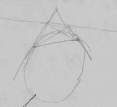
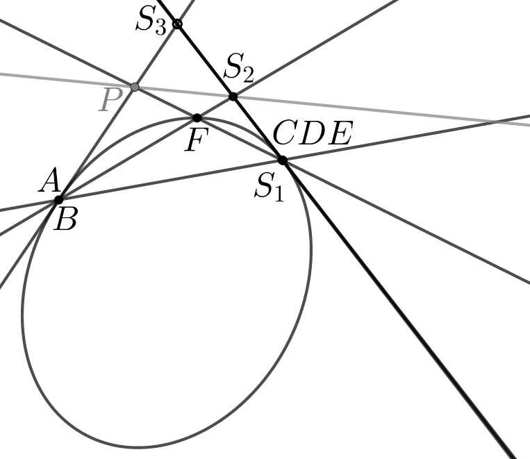
Figure 16: Parabolic involution on a conic. (a) Einstein’s sketch in the middle of manuscript page AEA 62-787r. Reproduced with permission from the Albert Einstein Archives. ©The Hebrew University of Jerusalem, Israel. Digital image photographed by Ardon Bar Hama. (b) Reconstruction of Einstein’s sketch. The gray objects were drawn by Einstein, but have no meaning in terms of involutions.

We get to this figure by moving the points $D=E$ and $C$ towards each other in figure 15. In this case, the points $C$, $D$, $E$, and $S_{1}$ fall together, see figure 16. Thus, the Pascal line passing through the points $S_{i}$ becomes a tangent, leading to the situation where only one invariant point exists. Since the center of the involution as intersection of the sides $CF$ and $AD$ falls together also with these points, every secant through the center of the involution passes through the point $C=D=E$. Thus, every point on the conic is a corresponding point to $C=D=E$ (parabolic involution). In the strict sense, this is not an involution anymore since it is not a one-to-one-correspondence (Coxeter,, 1961, 52). Nevertheless, we could describe the involution by $ACC\barwedge CAF$.

8 Projective Geometry Calculation in the Scratch Notebook

Figure 17: Einstein’s sketch probably related to the calculation on hyperbolic involutions. (a) Einstein’s fourth sketch in the Scratch Notebook. Reproduced with permission from the Albert Einstein Archives. ©The Hebrew University of Jerusalem, Israel. Digital image photographed by Ardon Bar Hama. (b) Einstein’s sketch with our suggested notation.

The fourth sketch of the double page in the Scratch Notebook, i.e the sketch at the top of the right hand side, is shown in figure 17(a). Beneath we find a short calculation and the sketch from figure 8(a) that we interpreted as the construction of pairs of an involution on a line. It is a priori not clear whether figure 17(a) is related at all to Einstein’s calculation, since it is a very generic sketch. But as we will show, imposing the notation from figure 17(b) enables us to connect the sketch directly with the calculation, while at the same time the drawn brace gets a meaning as correlating the two invariant points of an involution.

We assume that the points in figure 17(b) lie on one line and the coordinates of the points $O$, $X_{1}$, $A$, and $X_{2}$ be $0$, $x_{1}$, $a$, and $x_{2}$, respectively. A pair $x_{1}$, $x_{2}$ of an involution on this line can be described analytically by

$$rx_{1}x_{2}+s(x_{1}+x_{2})+t=0,$$ (1)

with real numbers $r$, $s$, and $t$ which completely describe the involution, see (Coxeter,, 1987, 118,151) or (Faulkner,, 1960, 36). Imposing the assumption that both $O$ and $A$ are invariant points, we get $t=0$ as well as $s=-a$ when setting $r=2$. Interpreting $X_{1}$ and $X_{2}$ as a pair of this involution, the relation

$$2x_{1}x_{2}-a(x_{1}+x_{2})=0$$ (2)

holds, which can be recast to read

$$\frac{x_{1}}{a-x_{1}}:\frac{x_{2}}{a-x_{2}}=-1.$$ (3)

Considering the cross ratio

$$(OA,X_{1}X_{2})=\frac{x_{2}-a}{x_{2}}:\frac{x_{1}-a}{x_{1}}$$ (4)

of the points $O$, $A$, $X_{1}$, and $X_{2}$ (Kaplansky,, 1969, 107), equation 3 implies that $O$ and $A$ are harmonic conjugates to $X_{1}$ and $X_{2}$. This result is no surprise since the two invariant points of a hyperbolic involution are harmonic conjugates to any other pair of the involution (Coxeter,, 1987, 47).

Einstein worked the calculation the other way around. Starting from equation 3 he derived equation 2. He then implicitly set $x=x_{1}=x_{2}$ and got

$$x^{2}-ax=0.$$ (5)

He concluded

$$x=0\;\text{and}\;x=a.$$ (6)

We summarize that Einstein started with the harmonic relation of four points with the coordinates $0$, $a$, $x_{1}$, and $x_{2}$ and recast this equation in order to get the equation of a hyperbolic involution. He then determined the two invariant points by setting $x=x_{1}=x_{2}$. He finished his calculation with a word that reads “Doppelv.” or “Doppelp.”, which could either stand for cross ratio or double point. The latter describes invariant points as in (Grassmann,, 1909, 111), (Enriques,, 1915, 68) or (Coxeter,, 1961, 32). As we know from Grossmann’s lecture notes, Fiedler used this term in his lecture attended by Einstein as well (Grossmann,, 1897, 71). Both cases fit to the context presented here as Einstein started with the cross ratio at the beginning and determined the invariant points of the involution at the end.

8.1 Similarities to the Manuscript Page AEA 62-785

On manuscript page AEA 62-785, Einstein made calculations on involutions using equation 1 as well. Just as we found the construction of pairs of an involution right next to Einstein’s calculation in the Scratch Notebook (see figure 8), Einstein constructed pairs of an involution on AEA 62-785, too. As we will see, he also constructed invariant pairs explicitly, analogous to the interpretation of figure 4 in section 6.3.

Einstein started with the equation of involution

$$axy+b(x+y)+c=0$$ (7)

with real numbers $a\neq 0$, $b$, and $c$. Einstein then investigated the corresponding point of the point at infinity. Letting $x$ be the point at infinity, we have

$$y=-\frac{b}{a}$$ (8)

for the corresponding point $y$. We can either see this by introducing homogeneous coordinates in the projective plane or, as Einstein apparently did, by setting $x=\infty$ after dividing equation 7 by $x$. By (Coxeter,, 1961, 121,122), this point $y$ is called the center of the involution. Einstein indicated that this point should be the origin. Setting $y=0$ yields $b=0$, as written down by Einstein.

For any pair $x_{1}$, $y_{1}$ of the involution, it thus is

$$x_{1}y_{1}+\widetilde{c}=0$$ (9)

with $\widetilde{c}=\nicefrac{{c}}{{a}}$. Einstein simply wrote down

$$xy+c=0,$$ (10)

implicitly changing the meaning of $c$. By the conditions imposed by Einstein, equation 10 describes the constant of the involution, saying that the product $x\cdot y$ of any pair $x$, $y$ is constant. In other words: The distance between the center of the involution and $x$ times the distance between the center of the involution and $y$ is constant (Coxeter,, 1961, 122).

Einstein concluded that setting $x=y$ gives two roots that can either be real or imaginary. We will see in figures 18 and 19 that Einstein investigated both cases by drawing sketches.

Underneath a horizontal line, Einstein wrote down

$$a:b:c=\begin{vmatrix}x_{1}+y_{1}&1\\ x_{2}+y_{2}&1\end{vmatrix}\hskip 1.70709pt\mathpunct{:}\hskip 1.70709pt\begin{vmatrix}1&x_{1}y_{1}\\ 1&x_{2}y_{2}\end{vmatrix}\hskip 1.70709pt\mathpunct{:}\hskip 1.70709pt\begin{vmatrix}x_{1}y_{1}&x_{1}+y_{1}\\ x_{2}y_{2}&x_{2}+y_{2}\end{vmatrix}.$$ (11)

As we already saw, an involution is determined by any two pairs $x_{1}$, $y_{1}$ and $x_{2}$, $y_{2}$ (Coxeter,, 1987, 45). It can easily be shown that in this case, the real numbers $a$, $b$, and $c$ can be written as shown in equation 11 when reading the colons not as divisions or homogeneous coordinates but simply as a symbol for separation of corresponding terms (Blaschke,, 1954, 74).

As in equation 8, Einstein now considered $y$ to be the corresponding point to the point at infinity ($x=\infty$) yielding

$$y=-\frac{b}{a}=-\frac{\begin{vmatrix}1&x_{1}x_{1}\\ 1&x_{2}y_{2}\end{vmatrix}}{\begin{vmatrix}x_{1}+y_{1}&1\\ x_{2}+y_{2}&1\end{vmatrix}}=+\frac{x_{2}y_{2}-x_{1}y_{1}}{x_{2}+y_{2}-x_{1}+y_{1}}.$$ (12)

As before, setting $y=0$ directly yields the constant of the involution.

On the same manuscript page, Einstein drew three sketches while one of these sketches obviously was not finished and crossed out. The first sketch is shown in figure 18(a).

Figure 18: Construction of pairs $x_{1}$, $y_{1}$ and $x_{2}$, $y_{2}$ of a hyperbolic involution on a line as well as construction of the invariant points. (a) Einstein’s first sketch on AEA 62-785r. Reproduced with permission from the Albert Einstein Archives. ©The Hebrew University of Jerusalem, Israel. Digital image photographed by Ardon Bar Hama. (b) Reconstruction of Einstein’s sketch. Einstein did not draw the gray circles.

Interpreting the line $r$ in figure 18(b) as the radical axis of the two circles defined by their intersections $R_{1}$ and $R_{2}$, it is

$$\overline{Ox_{1}}\cdot\overline{Oy_{1}}=\overline{Ox_{2}}\cdot\overline{Oy_{2}}.$$ (13)

This implies that any circle through $R_{1}$ and $R_{2}$ determines a pair $x_{i}$, $y_{i}$ of the involution on line $g$ with center $O$ by the intersections of this circle with $g$ corresponding to equation 10. The two gray circles in figure 18(b) are the only circles that pass through $R_{1}$ and $R_{2}$ and only touch line $g$. These two circles determine the two invariant points $S_{1}$ and $S_{2}$ of the (hyperbolic) involution, which were marked by Einstein. By equation 10, the distances between the invariant points and the center, respectively, are equal. Einstein indicated this by drawing a half-circle through the two invariant points with center $O$.

We summarize that Einstein constructed two pairs $x_{1}$, $y_{1}$ and $x_{2}$, $y_{2}$ of an involution with center $O$ as well as two real invariant points, clearly connected to the calculation above. As Einstein indicated in his calculation, the two invariant points could also be imaginary, leading to an elliptic involution. This case was considered by Einstein in figure 19(a), titled “In the imaginary case” by Einstein himself.

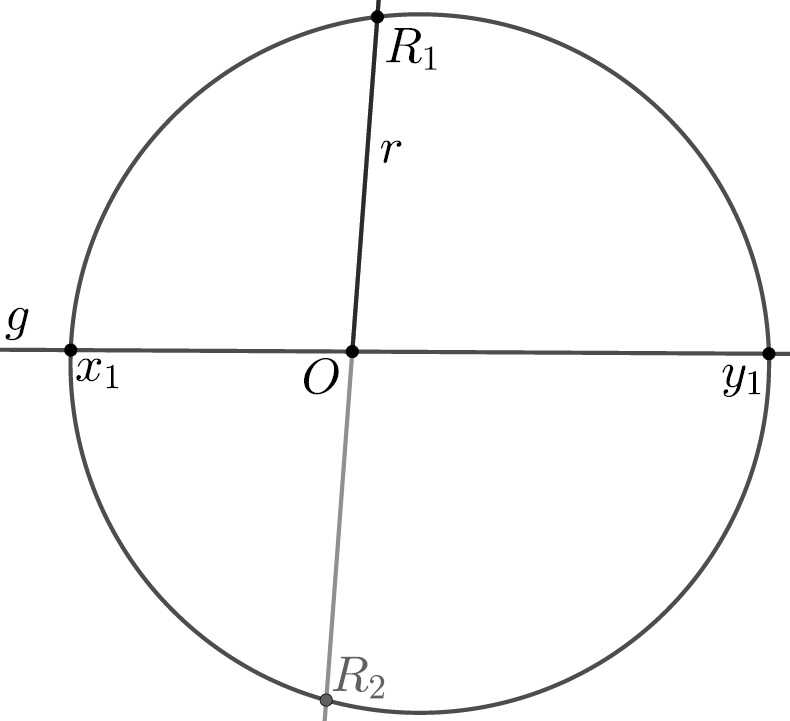
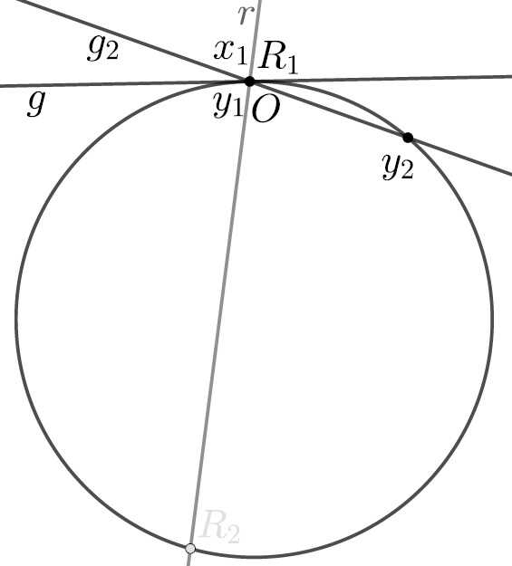
Figure 19: Construction of a pair $x_{1}$, $y_{1}$ of an elliptic and parabolic involution on a line. (a) Einstein’s second sketch on AEA 62-785r. Reproduced with permission from the Albert Einstein Archives. ©The Hebrew University of Jerusalem, Israel. Digital image photographed by Ardon Bar Hama. (b) Elliptic involution with no real invariant points; (c) Parabolic involution with one invariant point.

When moving up line $g$ in figure 18(b) such that it comes to lie between points $R_{1}$ and $R_{2}$, we arrive at the situation in figure 19(a), where Einstein did not draw the right circle anymore. Clearly, no circle through $R_{1}$ and $R_{2}$ exists that only touches line $g$, since all circles passing through $R_{1}$ and $R_{2}$ need to cross the line $g$ twice. Einstein did not draw point $R_{2}$. However, by his notation $x_{1}$, $O$, and $y_{1}$ it becomes clear that the pair $x_{1}$, $y_{1}$ is separated by the center $O$ corresponding to an involution where line $g$ passes between $R_{1}$ and $R_{2}$. In this case, the involution is elliptic, where no real invariant points exist. As we learn from Grossmann’s lecture notes on Projective Geometry held by Fiedler and attended by Einstein, the difference between hyperbolic and elliptic involutions was taught by Fiedler as we find it on this manuscript page (Grossmann,, 1897, 71):

[…] but those can be either real, then they are double points of the considered hyperbolic involution, or they are imaginary, such that the involution is elliptic.

Corresponding sketches can also be found in the lecture notes of Grossmann’s own lecture (Grossmann,, 1907, pp. 17.2 and 18.1).

As we see in figure 19(a), Einstein drew more lines as accounted for by our interpretation. Some of these lines are shown in figure 19(c). Here, the center of the involution falls together with the point $R_{1}$. We get to this situation when moving up line $g$ in figure 19(b). Thus, each circle that passes through $R_{1}$ and $R_{2}$ passes through the center of the involution, which is why every point on the line $g$ is a corresponding point to $O$. In particular, the circle drawn in figure 19(c) determines the only invariant point of this so called parabolic involution, such that $x_{1}$ and $x_{2}$ fall together.

Instead of drawing another circle through $R_{1}$ and $R_{2}$ in order to determine a second pair of the involution, we can also alter line $g$. See for example line $g_{2}$ that passes through the center $O$, too. Point $y_{2}$ now corresponds to $O$ as well as to any other point on the line. It is likely that Einstein first wanted to draw the case of the parabolic involution in a third sketch, but then added it to the second sketch after crossing out the third sketch.

We summarize that Einstein investigated hyperbolic, elliptic, and parabolic involutions on lines both algebraically and geometrically. The same involutions on conics instead of lines were investigated on manuscript page AEA 62-787r as we saw in section 7.1.

9 Further Sketches on AEA 124-446 and AEA 62-789

The first sketch on manuscript page AEA 124-446 has similarities to the third sketch on manuscript page AEA 62-789. Both sketches are shown in figure 20. As it was the case in section 6.2, these are very generic sketches that appear in different contexts as perspectivities, cross ratios (Enriques,, 1915, 106), involutions (Coxeter,, 1987, 62), imaginary elements (Dowling,, 1917, 139), or self-conjugate points (Coxeter,, 1987, 61).

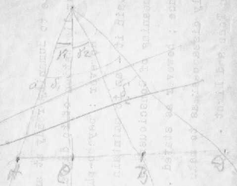
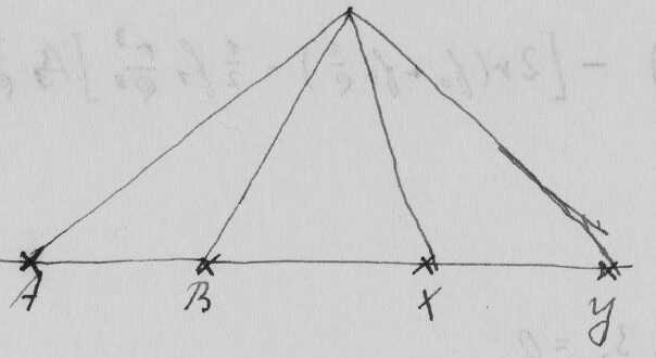
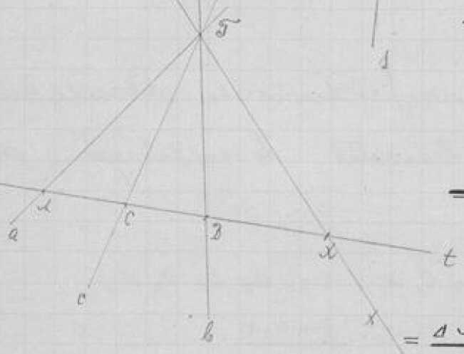
Figure 20: Similar sketches on projective geometry on manuscript pages AEA 124-446 and AEA 62-789r as well as in Grossmann’s lecture notes. (a) Einstein’s first sketch on the manuscript page AEA 124-446; (b) Einstein’s third sketch on manuscript page AEA 62-789; (c) Sketch from Grossmann’s lectures notes on “Darstellende Geometrie I”, original located at ETH. a) and b) are reproduced with permission from the Albert Einstein Archives. ©The Hebrew University of Jerusalem, Israel. Digital image photographed by Ardon Bar Hama.

On AEA 124-446, Einstein wrote down

$$\frac{AC}{BC}:\frac{AD}{BD}=\frac{BC}{AC}:\frac{BD}{AD}$$ (14)

and concluded

$$\frac{AC^{2}}{BC^{2}}:\frac{AD^{2}}{BD^{2}}=1.$$ (15)

We also find the expression

$$\frac{\sin{\gamma_{1}}}{\sin{\gamma_{2}}}:\frac{\sin{\delta_{1}}}{\sin{\delta_{2}}},$$ (16)

which is equal to the expressions in equation 14. Einstein canceled certain quantities as well as added some squares in retrospect. The relations above can easily be proven as in (Enriques,, 1915, 105-110) in the context of cross ratios. By Grossmann’s lecture notes, we know that Einstein already learned these relations in the winter semester 1896/97 when attending Fiedler’s lecture “Darstellende Geometrie I”, see (Grossmann, 6, 97, 38) and (Stachel,, 1987, 363). The corresponding sketch is shown in figure 20(c). The sketch on AEA 62-789 in figure 20(b) is very similar to these sketches, however, we do not find any related calculation on this manuscript page.

We also found a sketch on the reverse side of the letter AEA 6-250. It is remarkable that on this page, an equation is written down that is equivalent to an equation on AEA 62-789r which contains sketches on projective geometry as well, see section 6.2.

10 Alternative Interpretation

We already saw that the center of an involution has a special meaning as it determines pairs of the involution. By our interpretation, Einstein did not draw the center when considering Pascal’s theorem and its derivatives (except for figure 16, where it falls together with a vertex). We can entertain different interpretations such that the center of the involution can be identified explicitly. In that case, however, certain lines drawn by Einstein become meaningless.

Einstein’s sketches in figures 12(b) and 15(b), for instance, could also be interpreted as an involution that interchanges points $A$, $C$ and $D$, $F$, namely $ACD\barwedge CAF$. In this case, the point $S_{1}$ becomes the center of the involution since the secants $FD$ and $AC$ passing through $S_{1}$ determine two pairs of the involution. As $S_{1}$ is an interior point, the involution is an elliptic one. In this case, Einstein did not draw the Pascal line and, furthermore, the intersection $S_{3}$ of the tangents becomes meaningless.

Similarly, we could consider the involution $ADC\barwedge CFA$ instead of $ADC\barwedge DAF$ in figure 14(b). In this case, the intersection $S_{1}$ is the center of the involution. This point might have been drawn by Einstein in the section where the paper had been torn off. However, the construction via the line passing through $S_{1}$ and $S_{2}$ would have been unusual, since he did not draw the line $EF$. The axis of the involution then crosses the conic twice, which is why the involution is hyperbolic. As before, in this case, the intersection $S_{3}$ of the tangents in $A$ and $D$ would be meaningless.

We can also interpret Einstein’s sketch in figure 16 such that the center of the involution can be identified explicitly. Instead of looking at the parabolic involution $ACC\barwedge CAF$, we could consider the involution $FAD\barwedge DAF$ that interchanges the points $F$ and $D$ and let the point $A$ invariant. The center of the involution $P$ then is the intersection of the tangent in $A$ with the secant $DF$, which leads us to a hyperbolic involution. This interpretation, however, does not give a meaning to the line $PS_{2}$, either. Moreover, the intersection $S_{3}$ of the tangents in $A$ and $C$ would again be meaningless.

10.1 Manuscript Page AEA 62-785r

In section 8.1, we argued that Einstein considered hyperbolic, elliptic and parabolic involutions on lines that correspond to both the calculations on the same page and considerations on the manuscript page AEA 62-787r. However, for the sketch in figure 19(a) (see also figure 21(a)) another plausible interpretation is possible.

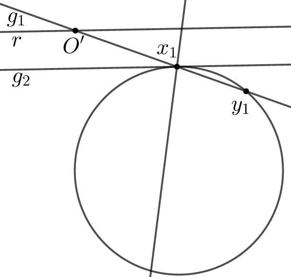
Figure 21: Alternative Interpretation for Einstein’s second sketch on AEA 62-785r. (a) Einstein’s second sketch on AEA 62-785r. Reproduced with permission from the Albert Einstein Archives. ©The Hebrew University of Jerusalem, Israel. Digital image photographed by Ardon Bar Hama. (b) Alternative Interpretation where the point at infinity is an invariant point.

We argued that Einstein implicitly assumed the point $R_{2}$ being on the circle such that the radical axis passes through the given circle. Then, we argued that the lines in figure 19(c) show the parabolic involution. Instead of this, we can argue also as follows: A radical axis can also be defined when the two circles do not meet each other. Assuming that the second circle is above the circle drawn in figure 21(a), the top horizontal line could be the radical axis (see the line $r$ in figure 21(b)). Let $O^{\prime}$ be the center of the involution on $g_{1}$, $x_{1}$ and $y_{1}$ is one corresponding pair. By rotating $g_{1}$ to $g_{2}$ around $x_{1}$, the point $O^{\prime}$ goes to infinity. As $O^{\prime}$ is the corresponding point to the point at infinity, it becomes an invariant point. In this case, $x_{1}$ becomes the second invariant point on the line $g_{2}$. This interpretation, however, does not fit to Einstein’s calculation where he set the center of the involution as origin (real point). However, it would provide an interpretation for the third horizontal line in figure 21(a).

11 A Conjecture on the Purpose of Einstein’s Ideas about Projective Involutions

Given any one of the sketches individually, it might be well possible that Einstein would simply have been doodling. But the network of relations between the sketches and calculations, both in the Scratch Notebook and in the Princeton manuscripts, and the relations between the notebook and the manuscripts pages, and the fact that all of these sketches and calculations could be connected to the notion of an involution strongly suggest that Einstein was doing the constructions and calculations with a certain purpose in mind. But what could that purpose have been?

It might be tempting to associate any explicit considerations of projective geometry on Einstein’s part with projective relativity of some form or other. Perhaps Einstein may have had in mind to interpret four-dimensional spacetime as some projected version of five-dimensional spacetime. Such association would be all the more justified by the fact that the relevant manuscript pages 62-785, 62-787, 62-789 all can be linked unambiguously to the Einstein-Bergmann correspondence around their five-dimensional generalization of Kaluza-Klein theory. However, we have not been able to establish any convincing link along these lines.

Instead, we would like to express a different conjecture about the heuristics of Einstein’s projective geometry sketches and calculations, as we have reconstructed them. We find equations that we can link to the correspondence between Einstein and Bergmann from summer 1938 on the three manuscript pages AEA 62-785r, 62-787r, and 62-789r. As it was stated in the follow-up of Einstein and Bergmann’s publication, Einstein tried to find particle-like solutions within the framework of his five-dimensional approach during that time (Einstein et al.,, 1941). We conjecture that in order to find these particle-like solutions, Einstein and Bergmann assumed a special parametrization of the five-dimensional metric, expressing periodicity with respect to the fifth coordinate, stationarity with respect to the (time-like) fourth coordinate and spatial (three-dimensional) spherical symmetry. Crucially, the spherical symmetry resulted in a dependence of the coefficients of the metric in terms of a radial coordinate $r$. Interpretation in terms of physical particles required regularity at the origin $r=0$ and a certain fall-off at (spatial) infinity $r\rightarrow\infty$. In order to satisfy the requirements, they considered power series expansions of the various coefficient functions. In this context, Einstein and Bergmann explicitly considered the mathematical problem to be that of an “expansion around the infinite point” (Einstein to Bergmann, Friday, i.e., probably 15 July 1938, AEA 6-242 and Bergmann to Einstein, 16 July 1938, AEA 6-264).

We therefore conjecture that the context of Einstein’s considerations of involution in projective geometry is motivated by the wish to gain a better understanding of properties of a power series expansion around infinity. Typically, an expansion around infinity is done by a transformation $z\rightarrow 1/z$ and expanding around $0$. This mapping is a special case of the general involution equation (1) or (7). Mapping the coordinates in such a way that the infinite point is mapped to a finite coordinate and by an involution, i.e. by a map that can be iterated to be inverted again would allow to investigate properties of the series expansion around infinity. The purpose of the considerations on involutions therefore may have been to consider a more sophisticated version of an expansion around infinity or to gain a geometric understanding of such a mapping. This conjecture will have to be tested against a more detailed reconstruction of Einstein’s attempts to construct particle solutions in the Einstein-Bergmann framework.

It is intriguing to note that the consideration of projective involutions in the Scratch Notebook appears sandwiched in calculations of the magnification factor of gravitational lenses where Einstein had also found a diverging expression on the page immediately preceding it. However, while the sketches and calculations on the Princeton manuscripts all indicate clearly Einstein’s interest in the infinite point, the infinite point does not appear explicitly in constructions of the Scratch Notebook.

12 Concluding Remarks

Our analysis shows, we believe, that Einstein maintained an active command of basic notions of projective geometry throughout his life even though this field of mathematics did not play a prominent role in his physical theories. It is remarkable that very similar constructions and calculations dealing with involutions in projective geometry can be found that were written down some quarter century apart. If our conjecture is right, the constructions reveal a creativity on Einstein’s part in working out solutions to unified field theory that have never made its way to published work. It will be interesting to further reconstruct the ideas documented in his research notes and working sheets.

References

- Askwith, (1917) Askwith, E. H. (1917). A Course of Pure Geometry. Cambridge University Press.
- Blaschke, (1954) Blaschke, W. (1954). Projektive Geometrie. Birkhäuser Verlag, 3 edition.
- Bracco, (2017) Bracco, C. (2017). Quand Albert devient Einstein. Paris: CNRS Editions.
- Buchwald et al., (2013) Buchwald, D. K., Renn, J., and Schlögl, R. (2013). A note on Einstein’s Scratch Notebook of 1910–1913. In Maas, A. and Schatz, H., editors, Physics as a Calling, pages 81–88. Leiden: Leiden University Press.
- Cahan, (2000) Cahan, D. (2000). The Young Einstein’s Physics Education: H.F.Weber, Hermann von Helmholtz, and the Zurich Polytechnic Physics Institute. In Howard, D. and Stachel, J., editors, Einstein: the formative years, 1879-1909, pages 43–82. Boston, Basel, Berlin: Birkhäuser.
- Coxeter, (1961) Coxeter, H. S. M. (1961). The Real Projective Plane. Cambridge University Press, 2 edition.
- Coxeter, (1987) Coxeter, H. S. M. (1987). Projective Geometry. Springer, 2 edition.
- Dowling, (1917) Dowling, L. W. (1917). Projective Geometry. Modern Mathematical Texts. McGraw-Hill Book Company, Inc.
- Dörrie, (1958) Dörrie, H. (1958). Triumph der Mathematik. Physica-Verlag, 5 edition.
- Einstein, (1949) Einstein, A. (1949). Autobiographisches. In Schilpp, P. A., editor, Albert Einstein: Philosopher-Scientist, pages 1–96. La Salle (Illinois): Open Court.
- Einstein, (1955) Einstein, A. (1955). Erinnerungen - Souvenirs. Schweizerische Hochschulzeitung. Sonderheft 100 Jahre ETH, 28:145–153.
- Einstein et al., (1941) Einstein, A., Bargmann, V., and Bergmann, P. G. (1941). On the five-dimensional representation of gravitation and electricity. In Theodore von Karman Anniversary Volume, pages 212–225. California Institute of Technology.
- Einstein and Bergmann, (1938) Einstein, A. and Bergmann, P. G. (1938). On a generalization of Kaluza’s theory of electricity. Annals of Mathematics, Second Series, 39(3):683–701.
- Einstein and Grossmann, (1913) Einstein, A. and Grossmann, M. (1913). Entwurf einer verallgemeinerten Relativitätstheorie und einer Theorie der Gravitation. Zeitschrift für Mathematik und Physik, 62(3):225–261. (Klein et al.,, 1995, Docs. 13, 26).
- Emch, (1905) Emch, A. (1905). An Introduction to Projective Geometry and its Applications. John Wiley & Sons; Chapman & Hall, Limited.
- Enriques, (1915) Enriques, F. (1915). Vorlesungen über Projektive Geometrie. B.G. Teubner Verlag, 2 edition.
- Faulkner, (1960) Faulkner, T. E. (1960). Projective Geometry. Oliver and Boyd.
- Fiedler, (1871) Fiedler, O. W. (1871). Die Darstellende Geometrie. Ein Grundriss für die Vorlesungen an technischen Hochschulen und zum Selbststudium. Leipzig: B.G. Teubner.
- Fiedler, (1883) Fiedler, O. W. (1883). Die darstellende Geometrie in organischer Verbindung mit der Geometrie der Lage. I. Theil. Die Methoden der darstellenden und die Elemente der projectivischen Geometrie. Leipzig: B.G.Teubner.
- Fiedler, (1885) Fiedler, O. W. (1885). Die darstellende Geometrie in organischer Verbindung mit der Geometrie der Lage. II. Theil. Die darstellende Geometrie der krummen Linien und Flächen. Leipzig: B.G.Teubner.
- Fiedler, (1888) Fiedler, O. W. (1888). Die darstellende Geometrie in organischer Verbindung mit der Geometrie der Lage. III. Theil. Die constituirende und analytische Geometrie der Lage. Leipzig: B.G.Teubner.
- Ganter and Rudio, (1888) Ganter, H. and Rudio, F. (1888). Die Elemente der analytischen Geometrie der Ebene. Zum Gebrauch an höheren Lehranstalten sowie zum Selbststudium dargestellt und mit zahlreichen Übungsbeispielen versehen. Leipzig: Teubner.
- Graf-Grossmann, (2015) Graf-Grossmann, C. E. (2015). Marcel Grossmann. Römerhof Verlag. Translation available in Graf-Grossmann, (2018).
- Graf-Grossmann, (2018) Graf-Grossmann, C. E. (2018). Marcel Grossmann. Springer International Publishing.
- Grassmann, (1909) Grassmann, H. E. (1909). Projektive Geometrie der Ebene. B.G. Teubner Verlag.
- Grossmann, 6 (97) Grossmann, M. (1896-97). Darstellende Geometrie I. ETH-Bibliothek Zürich, Hs 421:10.1.
- Grossmann, (1897) Grossmann, M. (1897). Projektivische Geometrie: Geometrie der Lage. ETH-Bibliothek Zürich, Hs 421:12.
- (28) Grossmann, M. (1898a). Geometrische Theorie der Invarianten I. ETH-Bibliothek Zürich, Hs 421:17.
- (29) Grossmann, M. (1898b). Infinitesimalgeometrie III. ETH-Bibliothek Zürich, Hs 421:16.
- Grossmann, (1907) Grossmann, M. (1907). Projektive Geometrie. ETH-Bibliothek Zürich, Hs 421:9.
- Hadamard, (1945) Hadamard, J. (1945). The Psychology of Invention in the Mathematical Field. Princeton: Princeton University Press.
- Hatton, (1913) Hatton, J. L. S. (1913). The Principles of Projective Geometry. Cambridge University Press.
- Heis and Eschweiler, (1878) Heis, E. and Eschweiler, T. J. (1878). Lehrbuch der Geometrie zum Gebrauche an höheren Lehranstalten. 4th rev. ed.Part 2. Stereometrie. Cologne: M. DuMont-Schauberg.
- Hunziker, (2005) Hunziker, H., editor (2005). Der jugendliche Einstein und Aarau. Basel: Birkhäuser.
- Janssen, (1999) Janssen, M. (1999). Rotation as the Nemesis of Einstein’s Entwurf Theory. In Goenner, H., Renn, J., Ritter, J., and Sauer, T., editors, The Expanding Worlds of General Relativity, pages 127–157. Boston, Basel, Berlin: Birkhäuser.
- Janssen et al., (2007) Janssen, M., D. Norton, J., Renn, J., Sauer, T., and Stachel, J. (2007). The Genesis of General Relativity, volume 1–2. Springer.
- Kaplansky, (1969) Kaplansky, I. (1969). Linear Algebra and Geometry. A Second Course. Allyn and Bacon.
- Kitz, (2015) Kitz, S. (2015). „Neuere Geometrie“ als Unterrichtsgegenstand der höheren Lehranstalten. ein Reformvorschlag und seine Umsetzung zwischen 1870 und 1920 . Ph.D. thesis, University of Wuppertal.
- (39) Klein, M. J., Kox, A. J., Renn, J., and Schulmann, R. (1993a). The Collected Papers of Albert Einstein, Volume 3: The Swiss Years: Writings, 1909-1911. Princeton University Press.
- Klein et al., (1995) Klein, M. J., Kox, A. J., Renn, J., and Schulmann, R. (1995). The Collected Papers of Albert Einstein, Volume 4: The Swiss Years: Writings, 1912-1914. Princeton University Press.
- (41) Klein, M. J., Kox, A. J., and Schulmann, R. (1993b). The Collected Papers of Albert Einstein, Volume 5: The Swiss Years: Correspondence, 1902-1914. Princeton University Press.
- Kormos Buchwald et al., (2015) Kormos Buchwald, D., Illy, J., Rosenkranz, Z., Sauer, T., and Moses, O., editors (2015). The Collected Papers of Albert Einstein, Volume 14: The Berlin Years: Writings & Correspondence, April 1923-May 1925. Collected Papers of Albert Einstein. Princeton University Press.
- Norton, (1984) Norton, J. D. (1984). How Einstein Found His Field Equations, 1912-1915. Historical Studies in the Physical Sciences, 14:253–316. reprinted in Einstein and the History of General Relativity, eds. D. Howard, J. Stachel (Boston et al.: Birkhäuser, 1989) pp. 101–159.
- Norton, (2000) Norton, J. D. (2000). ‘Nature is the Realisation of the Simplest Conceivable Mathematical Ideas’: Einstein and the Canon of Mathematical Simplicity. Studies in the History and Philosophy of Modern Physics, 31(2):135–170.
- Pyenson, (1980) Pyenson, L. (1980). Einstein’s Education: Mathematics and the Laws of Nature. ISIS, 71(258):399–425.
- Renn and Sauer, (1999) Renn, J. and Sauer, T. (1999). Heuristics and Mathematical Representation in Einstein’s Search for a Gravitational Field Equation. In Goenner, H., Renn, J., Ritter, J., and Sauer, T., editors, The Expanding Worlds of General Relativity, pages 87–125. Boston et al.: Birkhäuser.
- Renn et al., (1997) Renn, J., Sauer, T., and Stachel, J. (1997). The origin of gravitational lensing: A postscript to Einstein’s 1936 science paper. Science, 275(5297):184–186.
- Rowe, (2011) Rowe, D. E. (2011). Puzzles and paradoxes and their (sometimes) profounder implications. The Mathematical Intelligencer, 33(1):55–60.
- Sauer, (2008) Sauer, T. (2008). Nova geminorum 1912 and the origin of the idea of gravitational lensing. Archive for History of Exact Sciences, 62(1):1–22.
- Sauer, (2015) Sauer, T. (2015). Marcel Grossmann and his contribution to the general theory of relativity. In Proceedings of The Thirteenth Marcel Grossmann Meeting, pages 456–503. World Scientific Publishing.
- Sauer, (2019) Sauer, T. (2019). Einstein’s working sheets and his search for a unified field theory. The European Physical Journal H, pages 1–9.
- Sauer and Schütz, (2019) Sauer, T. and Schütz, T. (2019). Exploring gravitational lensing. European Journal of Physics, 40(3):035301.
- Sauer and Schütz, (2020) Sauer, T. and Schütz, T. (2020). Einstein’s Washington Manuscript on Unified Field Theory. Berichte zur Wissenschaftsgeschichte, in press. arxiv.org/2008.10005.
- Schubert, (1898) Schubert, H. (1898). Mathematische Mußestunden. Teubner.
- Sickenberger, (1888) Sickenberger, A. (1888). Leitfaden der elementaren Mathematik. Part 2, Planimetrie. Munich: Theodor Ackermann.
- Spieker, (1890) Spieker, T. (1890). Lehrbuch der ebenen Geometrie. Mit Übungs-Aufgaben für höhere Lehranstalten. Potsdam: Aug. Stein. 19th impr.edition.
- Stachel, (1987) Stachel, J., editor (1987). The Collected Papers of Albert Einstein, Volume 1: The Early Years, 1879-1902. Princeton University Press.
- Stachel, (1996) Stachel, J. (1996). Albert Einstein and Mileva Maric: A Collaboration That Failed to Develop. In Abir-Am, P. and Pycior, H., editors, Creative Couples in Science, pages 207–219. New Brunswick: Rutgers University Press.
- Troemel-Ploetz, (1990) Troemel-Ploetz, S. (1990). Mileva Einstein-Marić: The woman who did Einstein’s mathematics. Index on Censorship, 9:33–36.
- Van Dongen, (2002) Van Dongen, J. (2002). Einstein and the Kaluza-Klein Particle. Studies in History and Philosophy of Modern Physics, 33:185–210.
- Van Dongen, (2010) Van Dongen, J. (2010). Einstein’s Unification. Cambridge University Press.
- (62) Veblen, O. and Young, J. W. (1910a). Projective Geometry Vol. 1. Boston etc.: Ginn and Company.
- (63) Veblen, O. and Young, J. W. (1910b). Projective Geometry Vol. 2. Boston etc.: Ginn and Company.
- Volkert, (2020) Volkert, K. (2020). Wilhelm Fiedlers „Darstellende Geometrie“. Preprint. to appear.
- Zahar, (1980) Zahar, E. (1980). Einstein, Meyerson and the Role of Mathematics in Physical Discovery. British Journal for the Philosophy of Science, 31.