First and second-order dust-ion-acoustic rogue waves in non-thermal plasma

Abstract

A nonlinear Schrödinger equation (NLSE) has been derived by employing reductive perturbation method for investigating the modulational instability of dust-ion-acoustic waves (DIAWs) in a four-component plasma having stationary negatively charged dust grains, inertial warm ions, and inertialess non-thermal electrons and positrons. It is observed that under consideration, the plasma system supports both modulationally stable and unstable domains, which are determined by the sign of the dispersive and nonlinear coefficients of NLSE, of the DIAWs. It is also found that the nonlinearity as well as the height and width of the first and second-order rogue waves increases with the non-thermality of electron and positron. The relevancy of our present investigation to the observations in space plasmas is pinpointed.

1 Introduction

The existence of massive dust grains in different electron-positron-ion (EPI) plasmas (viz., Jupiter’s magnetosphere [1], Milky Way [2], auroral zone [3], accretion disks near neutron stars [2], the hot spots on dust rings in the galactic centre [3, 4, 5, 6], interstellar medium [2], and around pulsars [5], etc.) does not only change the dynamics of the plasma medium but also significantly modifies the basic properties of electrostatic dust-acoustic (DA) waves (DAWs) [5, 6, 7] and dust-ion-acoustic (DIA) waves (DIAWs) [1, 2, 3]. Esfandyari-Kalejahi et al. [7] studied large amplitude DA solitary waves in EPI plasma, and demonstrated that the amplitude of the DA solitary waves increases with the charge state of dust grains. El-Tantawy et al. [8] investigated DIAWs in EPI dusty plasma medium (EPIDPM), and observed that the amplitude and width of the positive potential increases with the number density and charge state of the dust grains.

The signature of non-thermal electrons in space plasmas has been observed by the Viking [9] and Freja satellites [10]. Cairns et al. [11] first introduced non-thermal distribution and associated parameter $\alpha$ demonstrating the measurement of deviation from Maxwellian distribution for explaining the high-energy tails in space plasmas. Banerjee and Maitra [3] investigated DIA solitons and double layers in presence of non-thermal positrons and electrons. Paul et al. [4] considered a four-component plasma model having warm ions, stationary dust grains, non-thermal electrons and positrons, and studied DIAWs, and found that the system supports only positive potential super-solitons.

The modulational instability (MI) of electrostatic waves and formation of associated rogue waves (RWs) have been governed by the nonlinear Schrödinger equation (NLSE). A number of authors studied the MI of various kind of waves in different plasma medium [12, 13, 14, 15, 16, 17]. Guo et al. [14] investigated the MI of DIAWs in EPIDPM in presence of non-extensive electrons and positrons. Bains et al. [15] considered iso-thermal electrons and positrons to observe the MI condition of DIAWs, and found that the critical wave number decreases with ion temperature. El-Labany et al. [16] studied the MI of DAWs in a three-component plasma medium having non-thermal plasma species, and found that the height of the DA RWs (DARWs) increases with the non-thermality of plasma species. El-Tantawy et al. [17] examined ion-acoustic (IA) super RWs in a two-component non-thermal plasma having inertial ions and inerialess electrons, and reported that the nonlinearity as well as MI growth rate of the IA waves increases with the non-thermality of electrons. To the best of our knowledge, the effects of non-thermal electrons and positrons, and stationary negatively charged massive dust grains on the MI of DIAWs and associated DIA RWs (DIARWs) have not yet been investigated. Therefore, in our present work, we will examine the MI of DIAWs and associated DIARWs in a four-component EPIDPM.

The manuscript is organized in the following order: The basic governing equations are presented in Section 2. The derivation of the NLSE is demonstrated in Section 3. The MI of DIAWs is provided in Section 4. The DIARWs are exhibited in Section 5. Finally, the conclusion is presented in Section 6.

2 Model Equations

We consider a four-component unmagnetized plasma model having inertial warm ions, inertialess non-thermal electrons and positrons, and stationary negatively charged massive dust grains. At equilibrium, the quasi-neutrality condition can be expressed as $n_{e0}+Z_{d}n_{d0}=n_{p0}+Z_{i}n_{i0}$, where $n_{e0}$, $n_{d0}$, $n_{p0}$, and $n_{i0}$ are, respectively, the equilibrium number densities of electrons, dust grains, positrons, and ions. $Z_{i}$ is the charge state of the positive ion and $Z_{d}$ is the number of electrons residing on the dust grains surface. The normalized governing equations can be written in the following form

$$\frac{\partial n_{+}}{\partial t}+\frac{\partial}{\partial x}(n_{+}u_{+})=0,$$ (1)

$$\frac{\partial u_{+}}{\partial t}+u_{+}\frac{\partial u_{+}}{\partial x}+\sigma n_{+}\frac{\partial n_{+}}{\partial x}=-\frac{\partial\phi}{\partial x},$$ (2)

$$\frac{\partial^{2}\phi}{\partial x^{2}}=\mu_{e}n_{e}+\mu_{d}-n_{+}-(\mu_{e}+\mu_{d}-1)n_{p},\$$ (3)

where $n_{+}$ is the warm ions number density normalized by it’s equilibrium value $n_{+0}$; $u_{+}$ is the ion fluid speed normalized by the IA wave speed $C_{+}=(Z_{+}k_{B}T_{e}/m_{+})^{1/2}$ (with $T_{e}$ being the electron temperature, $m_{+}$ being the ion mass, and $k_{B}$ being the Boltzmann constant); $\phi$ is the electrostatic wave potential normalized by $k_{B}T_{e}/e$ (with $e$ being the magnitude of single electron charge); the time and space variables are normalized by $\omega_{p+}^{-1}=(m_{+}/4\pi Z_{+}^{2}e^{2}n_{+0})^{1/2}$ and $\lambda_{D+}=(k_{B}T_{+}/4\pi Z_{+}n_{+0}e^{2})^{1/2}$, respectively, and $T_{+}$ being the ion temperature; $p_{+}=p_{+0}(N_{+}/n_{+0})^{\gamma}$ [with $p_{+0}$ being the equilibrium adiabatic pressure of the ion, and $\gamma=(N+2)/N$, where $N$ is the degree of freedom. For one-dimensional case: $N=1$ then $\gamma=3$, and $p_{+0}=n_{+0}k_{B}T_{+}$]. Other plasma parameters are considered as $\sigma=3T_{+}/Z_{+}T_{e}$, $\mu_{e}=n_{e0}/Z_{+}n_{+0}$, and $\mu_{d}=Z_{d}n_{d0}/Z_{+}n_{+0}$. The expression for the number density of electron (following the Cairns’ non-thermal distribution [11, 18]) can be written as

$$n_{e}=\Bigg{[}1-\frac{4\alpha_{e}}{1+3\alpha_{e}}\phi+\frac{4\alpha_{e}}{1+3\alpha_{e}}\phi^{2}\Bigg{]}\mbox{exp}(\phi),$$

$$=1+F_{1}\phi+F_{2}\phi^{2}+F_{3}\phi^{3}+\cdot\cdot\cdot,\$$ (4)

where $F_{1}=(1-\alpha_{e})/(1+3\alpha_{e})$, $F_{2}=1/2$, $F_{3}=(15\alpha_{e}+1)/(18\alpha_{e}+6)$, and $\alpha_{e}$ being the non-thermality of electrons. The number density of positron (following the Cairns’ non-thermal distribution [11, 18]) can be written as

$$n_{p}=\Bigg{[}1+\frac{4\alpha_{p}}{1+3\alpha_{p}}\delta\phi+\frac{4\alpha_{p}}{1+3\alpha_{p}}\delta^{2}\phi^{2}\Bigg{]}\mbox{exp}(-\delta\phi),$$

$$=1+F_{4}\phi+F_{5}\phi^{2}+F_{6}\phi^{3}+\cdot\cdot\cdot,\$$ (5)

where $F_{4}=[(\alpha_{p}-1)\delta]/(1+3\alpha_{p})$, $F_{5}=\delta^{2}/2$, $F_{6}=[(15\alpha_{p}+1)\delta^{3}]/(18\alpha_{p}+6)$, and $\alpha_{p}$ being the non-thermality of positrons. The ratio of $T_{e}$ to $T_{p}$ (positron temperature) is defined by $\delta=T_{e}/T_{p}$. By substituting Eq. (4) and (5) into Eq. (3) and expanding up to third order in $\phi$, we can write

$$\frac{\partial^{2}\phi}{\partial x^{2}}+n_{+}=1+\mu_{d}+F_{7}\phi+F_{8}\phi^{2}+F_{9}\phi^{3}+\cdot\cdot\cdot,\$$ (6)

where

$$F_{8}=\frac{\mu_{e}-\eta\delta^{2}}{2},$$

$$F_{7}=\frac{\mu_{e}(1-\alpha_{e})(1+3\alpha_{p})-\eta(\alpha_{p}-1)(1+3\alpha_{e})\delta}{(1+3\alpha_{e})(1+3\alpha_{p})},$$

$$F_{9}=\frac{\mu_{e}(15\alpha_{e}+1)(18\alpha_{p}+6)+\eta(15\alpha_{p}+1)(18\alpha_{e}+6)\delta^{3}}{(18\alpha_{e}+6)(18\alpha_{p}+6)},\$$

where $\eta=\mu_{e}+\mu_{d}-1$, and the terms containing $F_{7}$, $F_{8}$, and $F_{9}$ in Eq. (6) are due to the contribution of the non-thermal electrons and positrons.

3 Derivation of the NLSE

To study the MI of DIAWs, we will derive a standard NLSE by employing the reductive perturbation method. So, we first introduce the stretched co-ordinates [18, 19]

$$\xi=\epsilon(x-v_{g}t),$$ (7)

$$\tau=\epsilon^{2}t,\$$ (8)

where $v_{g}$ is the group speed and $\epsilon$ is a small parameter. We can write the dependent variables as [20, 21, 22, 23]

$$n_{+}=1+\sum_{m=1}^{\infty}\epsilon^{m}\sum_{l=-\infty}^{\infty}n_{+l}^{(m)}(\xi,\tau)\mbox{exp}[il(kx-\omega t)],$$ (9)

$$u_{+}=\sum_{m=1}^{\infty}\epsilon^{m}\sum_{l=-\infty}^{\infty}u_{+l}^{(m)}(\xi,\tau)\mbox{exp}[il(kx-\omega t)],$$ (10)

$$\phi=\sum_{m=1}^{\infty}\epsilon^{m}\sum_{l=-\infty}^{\infty}\phi_{l}^{(m)}(\xi,\tau)\mbox{exp}[il(kx-\omega t)],\$$ (11)

where $k$ ($\omega$) is real variable representing the carrier wave number (frequency). The derivative operators in the above equations are treated as follows [24, 25, 26, 27]:

$$\frac{\partial}{\partial x}\rightarrow\frac{\partial}{\partial x}+\epsilon\frac{\partial}{\partial\xi},$$ (12)

$$\frac{\partial}{\partial t}\rightarrow\frac{\partial}{\partial t}-\epsilon v_{g}\frac{\partial}{\partial\xi}+\epsilon^{2}\frac{\partial}{\partial\tau}.\$$ (13)

Now, by substituting Eqs. (7)$-$(13), into Eqs. (1), (2), and (6), and selecting the terms containing $\epsilon$, the first order ($m=1$ and $l=1$) reduced equations can provide the dispersion relation of DIAWs

$$\omega^{2}=\frac{k^{2}}{k^{2}+F_{7}}+\sigma k^{2}.\$$ (14)

We again consider the second harmonic with ($m=2$ and $l=1$) and with the compatibility condition, we have obtained the group velocity of DIAWs

$$v_{g}=\frac{\omega^{2}-\beta^{2}}{k\omega},\$$ (15)

where $\beta=\omega^{2}-\sigma k^{2}$. The amplitude of the second-order harmonics is found to be proportional to $|\phi_{1}^{(1)}|^{2}$

$$n_{+2}^{(2)}=F_{10}|\phi_{1}^{(1)}|^{2},~{}~{}~{}~{}~{}n_{+0}^{(2)}=F_{13}|\phi_{1}^{(1)}|^{2},$$ (16)

$$u_{+2}^{(2)}=F_{11}|\phi_{1}^{(1)}|^{2},~{}~{}~{}~{}~{}u_{+0}^{(2)}=F_{14}|\phi_{1}^{(1)}|^{2},$$ (17)

$$\phi_{2}^{(2)}=F_{12}|\phi_{1}^{(1)}|^{2},~{}~{}~{}~{}~{}\phi_{0}^{(2)}=F_{15}|\phi_{1}^{(1)}|^{2},\$$ (18)

where

$$F_{10}=\frac{\sigma k^{6}+3\omega^{2}k^{4}+2F_{12}\beta^{2}k^{2}}{2\beta^{3}},$$

$$F_{11}=\frac{\omega F_{10}\beta^{2}-\omega k^{4}}{k\beta^{2}},$$

$$F_{12}=\frac{k^{4}(3\omega^{2}+\sigma k^{2})-2F_{8}\beta^{3}}{2\beta^{2}[(4k^{2}+F_{7})\beta-k^{2}]},$$

$$F_{13}=\frac{2v_{g}\omega k^{3}+k^{2}\omega^{2}+\sigma k^{4}+F_{15}\beta^{2}}{(v_{g}^{2}-\sigma)\beta^{2}},$$

$$F_{14}=\frac{v_{g}F_{13}\beta^{2}-2\omega k^{3}}{\beta^{2}},$$

$$F_{15}=\frac{k^{2}(2\omega v_{g}k+\sigma k^{2}+\omega^{2})-2F_{8}(v_{g}^{2}-\sigma)\beta^{2}}{\beta^{2}[F_{7}(v_{g}^{2}-\sigma)-1]}.\$$

Finally, the third harmonic modes ($m=3$) and ($l=1$), with the help of Eqs. (14)$-$(18), give a set of equations, which can be reduced to the following NLSE:

$$i\frac{\partial\Phi}{\partial\tau}+P\frac{\partial^{2}\Phi}{\partial\xi^{2}}+Q\Phi|\Phi|^{2}=0,\$$ (19)

we have considered $\Phi$=$\phi_{1}^{(1)}$ for simplicity, and in Eq. (19), $P$ is the dispersion coefficient which can be written as

$$P=\frac{\beta(4\sigma\omega k^{2}-3v_{g}k\omega^{2}-\sigma v_{g}k^{3})}{2\omega^{2}k^{2}},\$$ (20)

and $Q$ is the nonlinear coefficient which can be written as

$$Q=\frac{\beta^{2}(3F_{9}+2F_{8}F_{12}+2F_{8}F_{15})-Q^{\prime}}{2\omega k^{2}},\$$ (21)

where $Q^{\prime}=k^{2}[(\sigma k^{2}+\omega^{2})(F_{10}+F_{13})+2\omega k(F_{11}+F_{14})]$. The space and time evolution of the DIAWs are directly governed by the coefficients $P$ and $Q$.

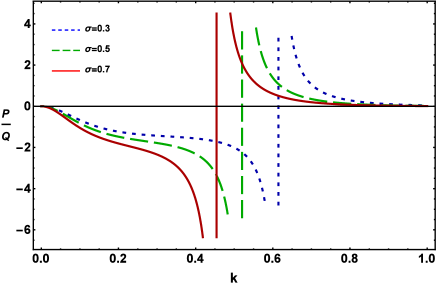
Figure 1: The variation of $P/Q$ with $k$ for different values of $\sigma$ when $\alpha_{e}=0.5$, $\alpha_{p}=0.5$, $\delta=1$, $\mu_{d}=0.02$, and $\mu_{e}=1.5$.

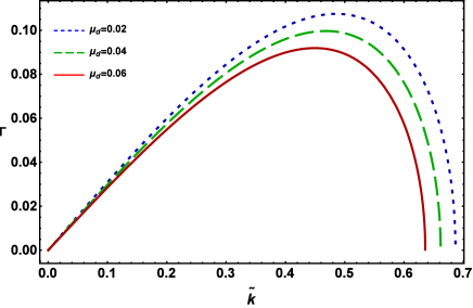
Figure 2: The variation of $\Gamma$ with $\widetilde{k}$ for different values of $\mu_{d}$ when $\alpha_{e}=0.5$, $\alpha_{p}=0.5$, $\delta=1$, $\mu_{e}=1.5$, $\sigma=0.3$, $\phi_{0}=0.5$, and $k=0.7$.

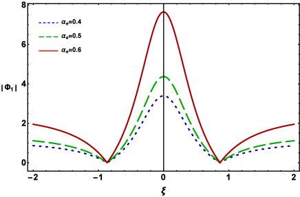
Figure 3: The variation of $|\phi_{1}|$ with $\xi$ for different values of $\alpha_{e}$ when $\alpha_{p}=0.5$, $\delta=1$, $\mu_{d}=0.02$, $\mu_{e}=1.5$, $\sigma=0.3$, $\tau=0$, and $k=0.7$.

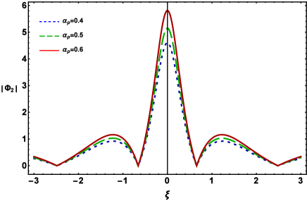
Figure 4: The variation of $|\phi_{2}|$ with $\xi$ for different values of $\alpha_{p}$ when $\alpha_{e}=0.5$, $\delta=1$, $\mu_{d}=0.02$, $\mu_{e}=1.5$, $\sigma=0.3$, $\tau=0$, and $k=0.7$.

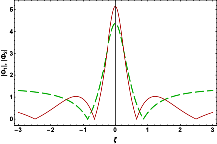
Figure 5: The variation of first-order (dashed green curve) and second-order (solid red curve) rational solutions of NLSE at $k=0.7$ and $\tau=0$.

4 Instability analysis

To study the MI of DIAWs, we consider the linear solution of the Eq. (19) in the form $\Phi=\widetilde{\Phi}e^{iQ|\widetilde{\Phi}|^{2}\tau}$+c.c., where $\widetilde{\Phi}=\widetilde{\Phi}_{0}+\epsilon\widetilde{\Phi}_{1}$ and $\widetilde{\Phi}_{1}=\widetilde{\Phi}_{1,0}e^{i(\widetilde{k}\xi-\widetilde{\omega}{\tau})}+c.c$. We note that the amplitude depends on the frequency, and that the perturbed wave number $\widetilde{k}$ and frequency $\widetilde{\omega}$ which are different from $k$ and $\omega$. Now, substituting these into Eq. (19), one can easily obtain the following nonlinear dispersion relation [18, 19]

$$\widetilde{\omega}^{2}=P^{2}\widetilde{k}^{2}\Big{(}\widetilde{k}^{2}-\frac{2|\widetilde{\Phi}_{0}|^{2}}{P/Q}\Big{)}.\$$ (22)

It is observed here that the ratio $P/Q$ is negative (i.e., $P/Q<0$), the DIAWs will be modulationally stable. On the other hand, if the ratio $P/Q$ is positive (i.e., $P/Q>0$), the DIAWs will be modulationally unstable. We have graphically examined the effect of temperature of the ion and electron as well as the charge state of the warm positive ion in recognizing the stable (i.e., $k<k_{c}$) and unstable (i.e., $k>k_{c}$) domains of DIAWs in Fig. 1, and it is clear from this figure that (a) the plasma system under consideration supports the DIAWs with either stable (i.e., $P/Q<0$) or unstable (i.e., $P/Q>0$); (b) the stable domain increases with the increase in the value of the charge state of the warm positive ion when $T_{+}$ and $T_{e}$ are invariant; (c) the $k_{c}$ decreases with the increase in the value of the ion temperature while increases with $T_{e}$ for a fixed value of $Z_{+}$, and this result agrees with the result of Bains et al. [15].

It is obvious from Eq. (22) that the DIAWs becomes modulationally unstable when $\widetilde{k}_{c}>\widetilde{k}$ in the regime $P/Q>0$, where $\widetilde{k}_{c}=\sqrt{2(Q/P)}{|\widetilde{\Phi}_{0}|}$. The growth rate $\Gamma$ of the modulationally unstable DIAWs is [14, 18, 19] given by

$$\Gamma=|P|\widetilde{k}^{2}\sqrt{\frac{\widetilde{k}_{c}^{2}}{\widetilde{k}^{2}}-1}.\$$ (23)

The variation of the $\Gamma$ with $\widetilde{k}$ for different values of $\mu_{d}$ can be seen in Fig. 2. It is obvious from this figure that (a) the maximum value of $\Gamma$ decreases (increases) with the increase in the values of $Z_{d}$ ($Z_{+}$) for a constant value of $n_{d0}$ and $n_{+0}$; (b) as we increase the value of $n_{d0}$ ($n_{+0}$), the maximum value of the $\Gamma$ decreases (increases) when $Z_{d}$ and $Z_{+}$ remain constant. The physics of this result is that the nonlinearity of the plasma system increases with the charge state and number density of the warm ion, but decreases with the charge state and number density of the stationary negatively charged massive dust grains.

5 Rogue waves

The NLSE (19) has a variety of rational solutions, among them there is a hierarchy of rational solution that are localized in both the $\xi$ and $\tau$ variables. The first-order rational solution of Eq. (19) can be written as [28]

$$\Phi_{1}(\xi,\tau)=\sqrt{\frac{2P}{Q}}\Big{[}\frac{4(1+4iP\tau)}{1+16P^{2}\tau^{2}+4\xi^{2}}-1\Big{]}\mbox{exp}(2iP\tau).\$$ (24)

Equation (24) reveals that a significant amount of DIAWs energy is concentrated into a comparatively small region in EPIDPM. We have numerically analysed Eq. (24) in Fig. 3 to illustrate the influence of non-thermal electrons on the formation of DIARWs, and it can be seen from the figure that (i) the height and width of the DIARWs increase as we increase in the value of non-thermality of the electrons (via $\alpha_{e}$); (ii) The physics of this result is that with increasing the value of $\alpha_{e}$, the nonlinearity of the plasma system is increasing, which leads to increase the height and the width of the DIARWs. This result agrees with the result of El-Labany et al. [16].

The interaction of the two or more first-order RWs can generate higher-order RWs which has a more complicated nonlinear structure. The second-order rational solution of Eq. (19) can be written as [28]

$$\Phi_{2}(\xi,\tau)=\sqrt{\frac{P}{Q}}\Big{[}1+\frac{G_{2}(\xi,\tau)+iM_{2}(\xi,\tau)}{D_{2}(\xi,\tau)}\Big{]}\mbox{exp}(i\tau P),\$$ (25)

where

$$G_{2}(\xi,\tau)=\frac{-\xi^{4}}{2}-6(P\xi\tau)^{2}-10(P\tau)^{4}$$

$$\hskip 5.69046pt-\frac{3\xi^{2}}{2}-9(P\tau)^{2}+\frac{3}{8},$$

$$M_{2}(\xi,\tau)=-P\tau\Big{[}\xi^{4}+4(P\xi\tau)^{2}+4(P\tau)^{4}$$

$$\hskip 5.69046pt-3\xi^{2}+2(P\tau)^{2}-\frac{15}{4}\Big{]},$$

$$D_{2}(\xi,\tau)=\frac{\xi^{6}}{12}+\frac{\xi^{4}(P\tau)^{2}}{2}+\xi^{2}(P\tau)^{4}$$

$$\hskip 5.69046pt+\frac{\xi^{4}}{8}+\frac{9(P\tau)^{4}}{2}-\frac{3(P\xi\tau)^{2}}{2}$$

$$\hskip 5.69046pt+\frac{9\xi^{2}}{16}+\frac{33(P\tau)^{2}}{8}+\frac{3}{32}.\$$

Figure 4 represents the second-order DIARWs associated with DIAWs in the modulationally unstable domain (i.e., $P/Q>0$). The increase in the value of $\alpha_{p}$ does not only cause to change the height of the DIARWs but also causes to change the width of the DIARWs. Figure 5 indicates the first-order and second-order solution of the NLSE at $\tau=0$, and it is clear from this figure that (a) the second-order rational solution has double structures compared with the first-order rational solution; (b) the height of the second-order rational solution is always greater than the height of the first-order rational solution; (c) the potential profile of the second-order rational solution becomes more spiky (i.e., the taller height and narrower width) than the first-order rational solution; (d) the second (first) order rational solution has four (two) zeros symmetrically located on the $\xi$-axis; (e) the second (first) order rational solution has three (one) local maxima.

6 Conclusion

In this study, we have performed a nonlinear analysis of DIAWs in an unmagnetized EPIDPM having stationary massive nagetively charged dust grains, inertial warm positive ions, and inertialess non-thermal Cairns’ distributed electrons and positrons. The evolution of DIAWs is governed by the standard NLSE, and the coefficients $P$ and $Q$ of NLSE can recognize the modulationally stable and unstable domains of DIAWs. It is observed that the critical wave number, for which the MI sets in, decreases with ion temperature but increases with electron temperature. The nonlinearity as well as the height and width of the DIARWs increases with the non-thermality of electrons and positrons. The limitation of this work is that the gravitational and magnetic fields are not consider. In future and for better understanding, someone can investigate the nonlinear propagation in a four-component EPIDPM by considering the gravitational and magnetic fields. However, these results may be applicable in understanding the conditions of the MI of DIAWs and associated DIARWs in Jupiter’s magnetosphere [1], Milky Way [2], auroral zone [3], accretion disks near neutron stars [2], the hot spots on dust rings in the galactic centre [3, 4, 5, 6], interstellar medium [2], and around pulsars [5], etc.

References

- [1] A. Paul and A. Bandyopadhyay, Astrophys Space Sci. 361, 172 (2016).
- [2] S. Sardar, et al., Phys. Plasmas 23, 073703 (2016).
- [3] G. Banerjee and S. Maitra, Phys. Plasmas 23, 123701 (2016).
- [4] A. Paul, et al., Phys. Plasmas 24, 013707 (2017).
- [5] N. Jehan, et al., Phys. Scr. 80, 035506 (2009).
- [6] E. Saberian, et al., Plasma Phys. Rep. 43, 83 (2017).
- [7] A. Esfandyari-Kalejahi, et al., Phys. Plasmas 19, 082308 (2012).
- [8] S.A. El-Tantawy, et al., Phys. Plasmas 18, 052113 (2011).
- [9] R. Boström, IEEE Trans. Plasma Sci. 20, 756 (1992).
- [10] P.O. Dovner, et al., Geophys. Res. Lett. 21, 1827 (1994).
- [11] R. Cairns, et al., J. Geophys. Res. 22, 2709 (1995).
- [12] I. Kourakis and P.K. Shukla, Phys. Plasmas 10, 3459 (2003).
- [13] R. Fedele, Phys. Scr. 65, 502 (2002).
- [14] S. Guo, et al., Ann. Phys. 332, 38 (2012).
- [15] A.S. Bains, et al., Astrophys Space Sci. 343, 293 (2013).
- [16] S.K. El-Labany, et al., Phys. Plasmas 22, 073702 (2015).
- [17] S.A. El-Tantawy, et al., Phys. Plasmas 20, 072102 (2013).
- [18] N.A. Chowdhury, et al., Chaos 27, 093105 (2017).
- [19] N.A. Chowdhury, et al., Phys. plasmas 24, 113701 (2017).
- [20] M.H. Rahman, et al., Phys. Plasmas 25, 102118 (2018).
- [21] N. Ahmed, et al., Chaos 28, 123107 (2018).
- [22] S. Jahan, et al., Commun. Theor. Phys. 71, 327 (2019).
- [23] M. Hassan, et al., Commun. Theor. Phys. 71, 1017 (2019).
- [24] R.K. Shikha, et al., Eur. Phys. J. D 73, 177 (2019).
- [25] M.H. Rahman, et al., Chinese J. Phys. 56, 2061 (2018).
- [26] N.A. Chowdhury, et al., Plasma Phys. Rep. 45, 459 (2019).
- [27] S.K. Paul, et al., Pramana-J. Phys. 94, 58 (2020).
- [28] A. Ankiewicz, et al., J. Phys. A 43, 12002 (2010).