Dispersion measure variability for 36 millisecond pulsars at 150 MHz with LOFAR

Abstract

Context. Radio pulses from pulsars are affected by plasma dispersion, which results in a frequency-dependent propagation delay. Variations in the magnitude of this effect lead to an additional source of red noise in pulsar timing experiments, including pulsar timing arrays that aim to detect nanohertz gravitational waves.

Aims. We aim to quantify the time-variable dispersion with much improved precision and characterise the spectrum of these variations.

Methods. We use the pulsar timing technique to obtain highly precise dispersion measure (DM) time series. Our dataset consists of observations of 36 millisecond pulsars, which were observed for up to 7.1 years with the LOFAR telescope at a centre frequency of $\sim 150$ MHz. Seventeen of these sources were observed with a weekly cadence, while the rest were observed at monthly cadence.

Results. We achieve a median DM precision of the order of $10^{-5}$ cm^-3 pc for a significant fraction of our sources. We detect significant variations of the DM in all pulsars with a median DM uncertainty of less than $2\times 10^{-4}$ cm^-3 pc. The noise contribution to pulsar timing experiments at higher frequencies is calculated to be at a level of 0.1–$10\text{\,}\mathrm{\SIUnitSymbolMicro s}$ at 1.4 GHz over a timespan of a few years, which is in many cases larger than the typical timing precision of $1\text{\,}\mathrm{\SIUnitSymbolMicro s}$ or better that PTAs aim for. We found no evidence for a dependence of DM on radio frequency for any of the sources in our sample.

Conclusions. The DM time series we obtained using LOFAR could in principle be used to correct higher-frequency data for the variations of the dispersive delay. However, there is currently the practical restriction that pulsars tend to provide either highly precise times of arrival at 1.4 GHz or a high DM precision at low frequencies, but not both, due to spectral properties. Combining the higher-frequency ToAs with those from LOFAR to measure the infinite-frequency ToA and DM would improve the result.

1 Introduction

Pulsars are highly magnetised, rapidly rotating neutron stars, the remnants of massive stars that ended their lives in a supernova explosion. Pulsars emit beams of electromagnetic radiation, pronounced mostly at radio frequencies, which sweep around in space as the neutron star rotates. If any of the beams cross the line of sight to the Earth, we detect regular pulses of radiation. While the shape of individual pulses can vary significantly, the average pulse shape, integrated over hundreds of pulses, is usually stable, which allows for a precise measurement of the ToAs of the integrated pulses.

There are two major distinct populations of pulsars: the canonical pulsars with pulse periods of the order of $\sim$0.1 s to $\sim$20 s and the MSPs, with typical spin periods of 1.4 ms to $\sim$30 ms. The latter were ‘spun up’ to shorter pulse periods by the transfer of mass and angular momentum from a binary stellar companion, which is why they are also called ‘recycled’ pulsars (Tauris et al. 2015). Millisecond pulsars are of particular scientific interest as the much shorter pulse periods allow for a more precise determination of the ToAs, and their rotation was found to be much more stable than that of canonical pulsars (Hobbs et al. 2010; Verbiest et al. 2009).

Pulsar timing.

The high rotational stability of pulsars, and MSPs in particular, together with the precise measurements afforded by pulsar timing, allows for extremely accurate modelling of the pulsar’s astrometric and astrophysical properties with a so-called timing model, a method called pulsar timing (see Lorimer & Kramer 2005). The model is usually evaluated by inspecting the timing residuals, that is, the difference between the measured ToAs of the pulses and the ones predicted by the model.

Pulsar timing arrays.

A major application of pulsars is in the so-called PTA projects, which aim to detect nanohertz frequency gravitational waves (see, e.g. Hobbs & Dai 2017; Tiburzi 2018; Burke-Spolaor et al. 2019). The basic idea behind these experiments is that passing gravitational waves would distort the spacetime around Earth in a way that the arrival times of some pulsars would be delayed, while the pulses of other pulsars arrive earlier at the telescope. By observing a large number of spatially separated, precisely timed pulsars over a time span of years to decades, a gravitational wave would be measurable in the spatial correlation of the timing residuals of different pulsars. One major focus of the PTAs is to detect a stochastic gravitational wave background signature such as the Hellings and Downs curve (Hellings & Downs 1983). This background is expected to be caused by inspiralling super-massive black hole binaries. To achieve a high precision in these experiments, many sources of noise have to be taken into account, including propagation effects in the ionised interstellar medium (IISM).

Influence of the interstellar medium.

The IISM is a cold plasma of ionised particles. An electromagnetic wave passing through this medium will experience a frequency-dependent change in group velocity, a phenomenon called dispersion. Specifically, this induces an additional delay $\Delta t$ in the ToAs, which can be approximated as (see Lorimer & Kramer 2005):

$$\Delta t=\frac{\rm DM}{k\nu^{2}},$$ (1)

where $k\simeq 2.41\times 10^{-4}$ cm^-3 pc MHz^-2 s^-1 is the dispersion constant, $\nu$ the observing frequency (expressed in MHz) and DM is the ‘dispersion measure’ (the integrated electron column density along the line of sight, expressed in cm^-3 pc), which is defined as:

$${\rm DM}=\int_{0}^{d}n_{\rm e}(l){\rm d}l,$$ (2)

where $d$ is the distance to the pulsar and $n_{\rm e}$ is the electron density.

The IISM is inhomogeneous, and so as our line of sight to the pulsar changes due to its proper motion, the Earth’s motion and the motion of the IISM we sample different regions of the IISM, which implies a temporal variability in the DM. The variations in the DM lead to a variable dispersive delay (see Eq. 1) and, thus, are a major source of noise in pulsar timing.

Using relatively high observing frequencies (¿ 1.4 GHz) minimises the impact of DM variations on the ToAs as the dispersive delay scales with $\nu^{-2}$ (see Eq. 1). However, the IISM turbulence spectrum is steep with significantly more power at larger scales (Armstrong et al. 1995), so for long timing campaigns, the dispersive delays will sooner or later still have a significant impact on the ToAs. Also, the observing frequency cannot be increased indefinitely, as pulsars have rather steep spectra (Maron et al. 2000), which leads to a loss of signal-to-noise ratio (S/N) at very high frequencies. Out of the 33 MSPs in their sample, Lazarus et al. (2016) selected 12 candidates with promising spectral indices to run test observations at 5 GHz (3 at 9 GHz). All the selected sources are detected, but the S/N is significantly lower than at 1.4 GHz, especially in the 9 GHz band. However, some of the sources have a sub-$\mathrm{\SIUnitSymbolMicro s}$ timing precision (post-fit RMS) at 5 GHz, so this approach can work for some flat-spectrum sources.

A more generally applicable solution is to correct for the time-variable dispersive delays by subtracting them from the ToAs, which effectively yields ToAs at infinite frequency. Dispersive delays can be measured either by using multi-frequency observations with several receivers, or by splitting wide-band observations into multiple sub-bands, but this kind of observation is not always available in PTA experiments (see, e.g. Desvignes et al. 2016). Also, the correction for the DM increases the uncertainty of the infinite-frequency ToA and this effect is especially large at high frequencies and small fractional bandwidths.

Another approach is to use low-frequency observations to measure the DM very precisely and use these measurements to correct the higher-frequency ToAs, which are often more sensitive and less affected by IISM effects. One potential complication of this approach is the possibility of frequency-dependent DMs (Cordes et al. 2016; Donner et al. 2019), which are caused by the fact that due to interstellar scattering, low-frequency observations effectively sample a larger volume of the IISM and are sensitive to IISM structures on a larger scale than at high frequencies. Therefore, dispersive delays measured at low frequency may not be representative for those experienced at high frequencies. Additionally, time-variable scattering can cause variations in the shape of the pulse profile that, if not corrected for, cause a frequency-dependent delay in the timing. While scattering induces a delay scaling with $\nu^{-4}$, some of its signature can be absorbed into a DM measurement, so this effect can cause a mismatch of the apparent DM at different frequencies.

In this paper, we present precise DM time series of 36 MSPs using low-frequency ($\sim$150 MHz) observations with a particular focus on pulsars used in PTA experiments. In Sect. 2 we describe our observational setup and our sources, while Sect. 3 explains our data analysis. We discuss our findings in Sect. 4 and present our conclusions in Sect. 5.

2 Observations

We used observations taken with the International Telescope (ILT) high-band antennas, described in detail by van Haarlem et al. (2013). Specifically, we used the data from two different pulsar monitoring campaigns, both of which are still ongoing. Campaign 1 uses the LOFAR Core stations situated in the north-east of the Netherlands to observe the sources of interest with monthly cadence for up to 7.1 years between 19 December 2012 and 14 January 2020. These data were coherently dedispersed and reduced using the pulsar pipeline (PulP) described by Stappers et al. (2011) and Kondratiev et al. (2016). It produces data cubes with resolution in frequency (195.3125 kHz-wide channels), time (10-sec sub-integrations), polarisation (four coherency products) and rotational phase (256 to 1024 phase bins). The data are stored in timer format, which is similar to the psrfits format described in Hotan et al. (2004). Each observation uses a centre frequency of 148.9 MHz, a bandwidth of 78.1 MHz (400 frequency channels) and lasts 5 to 30 minutes, depending on the brightness of the pulsars.

In Campaign 2, the six LOFAR stations of the German LOng Wavelength (GLOW) consortium, located in Effelsberg (telescope identifier DE601), Unterweilenbach (DE602), Tautenburg (DE603), Potsdam-Bornim (DE604), Jülich (DE605) and Norderstedt (DE609), were used as individual stand-alone telescopes, not connected to the ILT network. The beamformed data from the stations were sent to the MPIfR and the Forschungszentrum Jülich on dedicated high-speed links, where recording computers ran the dedicated und Pulsare (LuMP) data-taking software. LuMP formats and otherwise prepares the beamformed pulsar data for subsequent (off-line but near-real-time) phase-resolved averaging (commonly referred to as ‘folding’) using the dspsr software package (van Straten & Bailes 2011). This produces data cubes in the same format as PulP. The data we used from this campaign were taken between 20 August 2013 and 08 January 2020. The resulting dataset of these observations covers a time span of up to 6.4 years per pulsar, with a weekly cadence and typical integration times of 1 to 3 hours. Due to the difference in collecting areas (a factor of $\sim$10), the faintest pulsars were only observed with the Core and are not detectable with the international stations. Early observations and the observations of DE601 have a total bandwidth of 95.3 MHz (488 frequency channels), centred at 149.9 MHz. For technical reasons, the bandwidth of the other stations was reduced to 71.5 MHz (366 channels) in February 2015. In order to minimise the impact of the bandwidth reduction on the scientific quality of our data, the centre frequency was shifted to align the observed bandwidth with the most sensitive part of the bandpass, resulting in a new centre frequency of 153.8 MHz. This implies a shift in centre frequency by an integer number of frequency channels (20), so that the frequencies of individual channels remained constant over the entire dataset.

Table 1 shows detailed information on the observation characteristics for each source. We excluded PSR J1939+2134 (PSR B1937+21) from our analysis because its strongly variable scattering has a significant impact on the DM estimation (e.g. it shows the largest variation in scattering time of all sources in Levin et al. 2016). Also, due to the very strong scattering, the scattering tail of the pulse profile merges with the next pulse, so the profile is very wide (see Fig. 2 of Kondratiev et al. 2016). Observations of this pulsar at higher frequencies or more advanced analysis techniques like cyclic spectroscopy (Demorest 2011) could lead to more robust and similarly precise DM measurements.

Table 1: Summary of observations. Given are the pulsar name in J2000 coordinates, the pulse period $P$, the catalogue DM, the ecliptic latitude $\beta$, the total time span of the observations, the number of observations with GLOW and the LOFAR Core $N_{\text{glow}}$ and $N_{\text{core}}$, the median frequency-integrated ToA uncertainty, the median uncertainty of individual DM measurements, the median reduced $\chi^{2}$ of the individual DM fits, and the number of frequency channels in each observation. The last column shows whether the pulsar is used in different PTA projects (i.e. E: European Pulsar Timing Array, EPTA; P: Parkes Pulsar Timing Array, PPTA; N: North American Nanohertz Observatory for Gravitational Waves, NANOGrav; see Verbiest et al. 2016; Arzoumanian et al. 2018). A pulsar observed by any of the PTAs is also used by the International Pulsar Timing Array (IPTA).

source name	$P$	DM	$\beta$	span	$N_{\text{glow}}$	$N_{\text{core}}$	med($\sigma_{\text{ToA}}$)	med($\sigma_{\text{DM}}$)	med$\left(\frac{\chi^{2}}{n_{\text{free}}}\right)$	$N_{\text{chan}}$	PTA
(J2000)	(ms)	$\left(\frac{\text{pc}}{\text{cm}^{3}}\right)$	(deg)	(yrs)			($\mathrm{\SIUnitSymbolMicro s}$)	$\left(10^{-5}\frac{\text{pc}}{\text{cm}^{3}}\right)$
J0030+0451	$4.9$	$4.3$	$1.4$	$7.0$	355	79	7	16	$1.0$	10	E P N
J0034$-$0534	$1.9$	$13.8$	$-8.5$	$7.0$	1041	78	1	3	$1.0$	20	E P N
J0218+4232	$2.3$	$61.2$	$27.0$	$6.5$	539	74	13	35	$0.9$	10	E P N
J0407+1607	$25.7$	$35.6$	$-4.7$	$6.4$	386	65	24	56	$1.0$	10	-
J0621+1002	$28.9$	$36.5$	$-13.3$	$7.0$	10	74	251	568	$1.3$	10*	E P N
J0645+5158	$8.9$	$18.2$	$28.9$	$6.9$	268	4	3	7	$0.9$	10	E P N
J0740+6620	$2.9$	$15.0$	$44.1$	$4.8$	261	0	2	4	$0.9$	10	E P N
J0751+1807	$3.5$	$30.2$	$-2.8$	$7.1$	0	71	34	89	$0.6$	10*	E P N
J0952$-$0607	$1.4$	$22.4$	$-17.9$	$2.9$	37	33	9	14	$1.0$	8*	-
J1012+5307	$5.3$	$9.0$	$38.8$	$7.1$	1210	79	4	12	$1.2$	10	E P N
J1022+1001	$16.5$	$10.3$	$-0.1$	$7.1$	1224	80	5	12	$1.2$	20	E P N
J1024$-$0719	$5.2$	$6.5$	$-16.0$	$7.1$	5	81	32	80	$0.9$	8*	E P N
J1125+7819	$4.2$	$11.2$	$62.5$	$4.8$	282	0	3	8	$0.9$	10	E P N
aJ1300+1240a	$6.2$	$10.2$	$17.6$	$7.1$	377	80	3	7	$0.8$	20	-
J1400$-$1431	$3.1$	$4.9$	$-2.2$	$4.3$	145	49	7	6	$0.8$	8*	-
J1544+4937	$2.2$	$23.2$	$65.9$	$5.6$	5	53	19	59	$1.0$	6*	-
J1552+5437	$2.4$	$22.9$	$70.7$	$3.7$	0	41	3	7	$0.9$	10*	-
J1640+2224	$3.2$	$18.4$	$44.1$	$7.1$	435	79	7	18	$0.8$	8	E P N
J1658+3630	$33.0$	$3.0$	$58.7$	$2.6$	164	6	7	18	$0.9$	10	-
J1713+0747	$4.6$	$16.0$	$30.7$	$7.0$	7	79	12	29	$0.6$	10*	E P N
J1730$-$2304	$8.1$	$9.6$	$0.2$	$6.5$	0	74	21	49	$0.8$	10*	E P N
J1738+0333	$5.9$	$33.8$	$26.9$	$7.1$	0	77	39	110	$0.7$	6*	E P N
J1744$-$1134	$4.1$	$3.1$	$11.8$	$7.0$	372	79	14	19	$0.9$	10	E P N
J1853+1303	$4.1$	$30.6$	$35.7$	$6.5$	1	72	21	50	$0.8$	8*	E P N
bJ1857+0943b	$5.4$	$13.3$	$32.3$	$7.1$	0	75	41	82	$1.3$	10*	E P N
J1911$-$1114	$3.6$	$31.0$	$11.1$	$7.0$	0	74	32	68	$0.9$	10	E P N
J1918$-$0642	$7.6$	$26.6$	$15.4$	$7.0$	0	75	55	136	$0.8$	10*	E P N
J1923+2515	$3.8$	$18.9$	$46.7$	$6.6$	0	73	6	15	$0.9$	10*	E P N
J1944+0907	$5.2$	$24.4$	$29.9$	$6.5$	35	64	33	80	$0.8$	6*	E P N
cJ1955+2908c	$6.1$	$104.5$	$48.7$	$6.6$	0	74	100	273	$0.9$	10*	E P N
J2043+1711	$2.4$	$20.7$	$34.0$	$6.7$	3	71	6	17	$0.9$	10*	E P N
J2051$-$0827	$4.5$	$20.7$	$8.8$	$6.5$	6	74	14	29	$0.7$	10*	-
J2145$-$0750	$16.1$	$9.0$	$5.3$	$7.0$	1010	81	3	9	$1.1$	20	E P N
J2222$-$0137	$32.8$	$3.3$	$8.0$	$3.8$	130	41	22	49	$0.9$	10*	-
J2302+4442	$5.2$	$13.7$	$45.7$	$6.2$	0	71	20	51	$0.8$	10*	E P N
J2317+1439	$3.4$	$21.9$	$17.7$	$7.0$	381	77	2	6	$1.0$	10	E P N

* For these pulsars, an analytic standard template without frequency resolution was used.
      ^a PSR B1257+12
      ^b PSR B1855+09
      ^c PSR B1953+29

3 Data analysis

3.1 Pre-processing

The basic processing in this work has been carried out with the psrchive (Hotan et al. 2004; van Straten et al. 2012) software package. As a first step, the data were cleaned from radio frequency interference (RFI), by using a modified version of the ‘surgical’ algorithm of the clean.py script from the coastguard (Lazarus et al. 2016) python package to remove affected frequency channels and sub-integrations. In the rare case of outliers due to remaining RFI, the observations were also manually inspected and additional cleaning was applied using the psrchive program pazi. On average, 9.0% of data were removed in this process.

Pulse profiles can be polarisation dependent, so the total intensity profile can be significantly distorted if the different polarisation channels are not calibrated correctly, which affects the ToAs. As LOFAR antennas are static, there are several time-dependent projection effects to take into account. The data were calibrated in polarisation following the methods outlined in Noutsos et al. (2015) using the dreambeam python package to calculate the Jones matrices. For some pulsars (especially PSRs J1022+1001 and J2145$-$0750) this significantly improved the reduced $\chi^{2}$ values of the DM fits.

To make the dataset as homogeneous as possible, the bandwidth of all observations has been reduced to 70.3 MHz (i.e. 360 channels, centred at 153.2 MHz). To achieve this, two empty dummy channels had to be added at the top of the band for the LOFAR Core observations.

3.2 Timing

For the 20 pulsars also analysed by the International Pulsar Timing Array (IPTA), we took the timing model from the first IPTA data release (Verbiest et al. 2016, data combination B) and removed any existing DM models (including Solar wind) or FD parameters (which describe a frequency-dependent, non-dispersive delay in the timing residuals, see Arzoumanian et al. 2015), as we are interested in the time evolution of the DM and using frequency-resolved timing removes the need for FD parameters. To account for the different time span over which the IPTA ephemerides were derived, and because the DM estimates are expected to be more precise at the low radio frequencies of LOFAR, we performed an initial timing analysis over our dataset, with the aim of updating the reference DM for each pulsar. For this initial timing analysis, we derived an analytic template from a single, bright observation by fitting a series of von Mises functions (see, e.g. Jammalamadaka & SenGupta 2001) to the total intensity profile of the observation using the program paas. The functions are implemented in the form:

$$f(x)=A\cdot e^{\kappa\cdot(\cos(2\pi(x-\mu))-1)},$$ (3)

with $A$ being the amplitude of the component, $\kappa$ the compactness and $\mu$ the pulse phase. The phase $x$ is defined such that one full rotation corresponds to $x=1$. To obtain the ToAs, we used the fdm algorithm as implemented in the program pat on copies of our observations with reduced frequency resolution (integrated down to 10 frequency channels). Using these initial ToAs, we calculated the DM and its running average for each observation as described in Sect. 3.3, to be able to phase-align observations affected by DM variations.

For the 16 pulsars without a published IPTA timing model, we took our initial timing model from the ATNF Pulsar Catalogue (psrcat) by Manchester et al. (2005). For PSR J1658+3630, there was no timing model available in the catalogue, so we used the timing model from Sanidas et al. (2019). As these timing models often did not phase-align our dataset, we used the tempo2 software (Hobbs et al. 2006) to fit for parameters describing the pulsar’s rotation and, if needed, the position of the pulsar and its orbit in binary systems.

Using the optimised timing model and initial DM time series, we phase-aligned our dataset and created a standard pulse profile template for each pulsar by averaging only the observations from the observing site with the most observations of that pulsar. As the S/N of most observations is rather low (rarely above 100), we integrated the template in frequency to between 6 and 20 channels, depending on the pulsar’s S/N. We then applied a wavelet smoothing algorithm to the template with the program psrsmooth (Demorest et al. 2013), to avoid self-standarding (see Appendix A of Hotan et al. 2005). With this template, we again used the fdm algorithm to calculate the ToAs, matching each frequency channel of the observation (that was frequency-integrated accordingly) with the corresponding channel of the template. With this method, any constant frequency dependence of the pulse profile is modelled by the template and will not affect our measurement of DM.

If the templates generated in the procedure above were too noisy (due to low intrinsic flux of the pulsar and a small number of observations), the smoothing produced unphysical features in the profile shape. In these cases we used an analytic template without frequency resolution, created in the same way as in the initial analysis. In principle, this would imply the need of FD parameters in the timing model to account for the frequency-dependent profile shape, but in practice the frequency dependence is not significant, demonstrated by the median $\chi^{2}$ of the DM fits being close to unity (see Table 1).

3.3 Calculation of the DM

To get a precise time series of the DM, we used tempo2 to fit for DM for each observation individually. This approach avoids any correlation of the measured DMs with other (time-dependent) timing parameters. To mitigate the impact of outlier ToAs on our measured DM, we apply an automatic ToA rejection scheme as was done similarly in Tiburzi et al. (2019). We reject a ToA if its residual-to-uncertainty ratio $k$ is larger than four times the mean $k$. Specifically, we repeatedly applied the following rules until no ToA was removed in the iteration:

We calculated the timing residuals $r_{i}$ for each channel $i$ of a given observation using the tempo2 general2 plugin and noted the corresponding ToA uncertainties $\sigma_{i}$. The mean residual-to-uncertainty ratio is then calculated as $k=\text{mean}(|r_{i}|/\sigma_{i})$ and set to unity if the result was less than unity. If the condition $|r_{i}|/\sigma_{i}>4k$ was met for any of the residuals, we rejected the corresponding ToA. Finally, we fit for DM with tempo2.

The iterative process is necessary as the variable DM gives rise to significant structure in our frequency-resolved residuals, meaning that many are far from zero. This is also why the factor $k$ was introduced, as without it, ToAs at the edges of the band would be removed in the presence of a dispersive slope. The outliers were caused by a low S/N in the corresponding frequency channel, which can occur due to the pulsar being intrinsically faint at that frequency, short integration times, removal of large parts of that frequency range due to RFI, remaining low-level RFI or a combination of these. On average, 0.7% of the ToAs of an observation were removed during this step, mostly at the edges of the band where the telescope is less sensitive. We estimate that our outlier rejection procedure will produce fewer than ten false positives across our entire 36-pulsar dataset. While the median reduced $\chi^{2}$ of the final DM fits is close to unity for all pulsars in our sample (see Table 1) and the distribution is strongly peaked around 1, there are observations not following this distribution with reduced $\chi^{2}\gg 1$. These cases occured when most ToAs of an observation were flawed, usually because the pulsar was too faint or the entire observation was dominated by RFI. We excluded all DM measurements with a reduced $\chi^{2}>5$ from our subsequent analysis (on average 4% of all observations). Finally, we applied the standard tempo2 procedure of multiplying the DM uncertainty by the square root of the reduced $\chi^{2}$, because a high reduced $\chi^{2}$ indicates unmodelled structure or underestimated ToA uncertainties. To be conservative in our uncertainties and due to the low number of ToAs per fit, we only applied this procedure for fits with reduced $\chi^{2}>1$.

The resulting DM time series are shown in Figs. 1-3, with the reference DM of the standard template subtracted. The median DM precision for each source is shown in Table 1. As the median reduced $\chi^{2}$ is close to unity for all pulsars in our sample, the data are well fit by the model. From that we can rule out any significant frequency-dependent structure in the residuals or a frequency dependence of the DM as discussed in Donner et al. (2019), where we present a system with more extreme DM variations.

To improve our sensitivity to low-amplitude variations, we computed a running average of the DM time series. For each observation MJD, a weighted average over all observations was formed, weighting each DM value by the inverse of its variance. Additionally, the weights were reduced exponentially with time, scaled to $1/e$ of their original value over half the averaging window. We chose an averaging window of 30 days for pulsars with sharp features in their DM signal (i.e. PSRs J0030+0451, J0034$-$0534, J1022+1001, J1400$-$1431, J2145$-$0750, and J2317+1439) and 60 days for the rest.

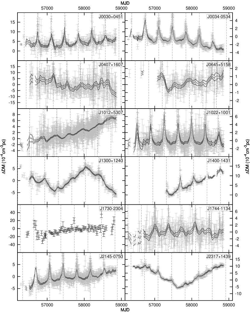
Figure 1: DM time series for 12 MSPs that show a detectable Solar wind signal. Individual DM measurements are plotted in grey, while running averages and their uncertainty are represented by solid grey and black lines, respectively. For faint pulsars only observed with the LOFAR core, the running average is not plotted due to the low observing cadence. Only points with uncertainties less than three times the median uncertainty are plotted. The vertical dashed grey lines indicate the epochs of minimum angular separation from the Sun.

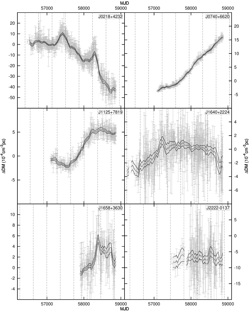
Figure 2: DM time series for six MSPs that were regularly observed with GLOW and do not show a clear Solar wind signal. The representation is the same as in Fig. 1.

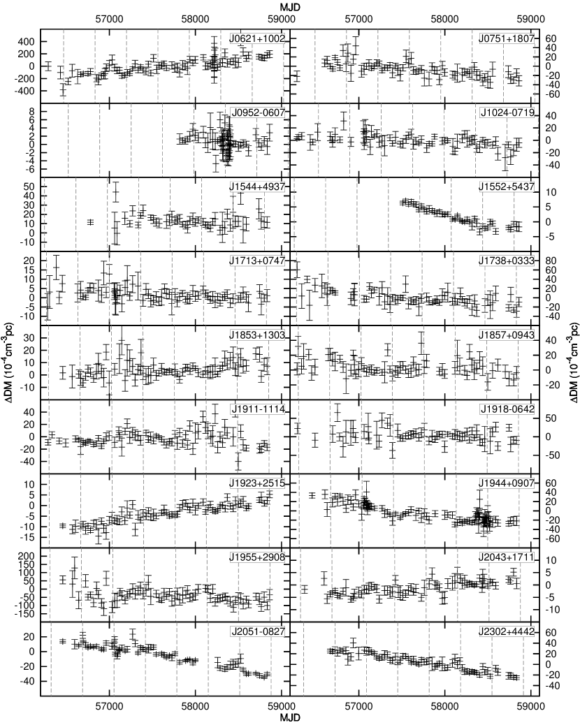
Figure 3: DM time series for 18 faint MSPs that are only monitored regularly with the LOFAR Core and do not show a clear Solar wind signal. The representation is the same as in Fig. 1.

4 Discussion

Most of the pulsars in our sample show DM variability, on diverse timescales. The amplitude of these variations ranges from $\sim 10^{-4}$ cm^-3 pc to $10^{-3}$ cm^-3 pc over several years or less. Pulsars that do not show DM variations (e.g. PSR J1853+1303) are very faint at LOFAR frequencies, with a single-observation DM uncertainty of $2\times 10^{-4}$ cm^-3 pc or worse, so the non-detection of variations may be caused by a lack of sensitivity, and variations of the order of a few $10^{-4}$ cm^-3 pc cannot be ruled out.

4.1 Solar wind

We detect the DM variations due to the Solar wind in 12 pulsars, namely PSRs J0030+0451, J0034$-$0534, J0407+1607, J0645+5158, J1012+5307, J1022+1001, J1300+1240, J1400$-$1438, J1730$-$2304, J1744$-$1134, J2145$-$0750, and J2317+1439 (see Fig. 1). The angular distance of these sources from the ecliptic ranges from 0.1° (PSR J1022+1001) to 38.8° (PSR J1012+5307, see Table 1). We note that for PSR J1730$-$2304, there are only a few observations close to the Sun due to the low observing cadence with the LOFAR Core and thus those observations clearly stand out from the rest of the DM measurements. For some pulsars with low (¡$10\degree$) absolute ecliptic latitude, we do not clearly see the impact of the Solar wind due to a lack of measurement precision: PSRs J0751+1807, J2051$-$0827, and J2222$-$0137.

As shown in Tiburzi et al. (2019), the widely used Solar wind models are insufficient to correctly account for the highly variable Solar wind, which leads to short-term variations in the residual DMs of the order of a few $10^{-4}$ cm^-3 pc, even at larger separations from the Sun (up to $\sim 50\degree$). From our study, we can confirm that a spherical model with constant amplitude (as is usually applied) does not suffice in most cases. This becomes clear in Fig. 1, where the amplitude of the Solar wind strongly varies from year to year, which is expected due to the variable Solar activity. Further analysis of the Solar wind impact on these data will be presented by Tiburzi et al. (in prep).

4.2 Observed DM variations

Lam et al. (2018) report a DM event in PSR J1713+0747 around MJD 57510, where the DM temporarily drops by about $4\times 10^{-4}$ cm^-3 pc. There is no indication of this event in our LOFAR DM time series (see Fig. 3). This can partly be explained by a lack of sensitivity as our DM precision is similar to the amplitude of the event. Additionally, the event is observed at higher frequencies and could be partly smeared at lower frequencies due to a frequency-dependent DM, as discussed in Cordes et al. (2016).

Some sources show very linear gradients in DM, for example PSRs J0740+6620, J1552+5437, and J1400$-$1431, the last of which is also affected by the Solar wind. While these linear trends are unlikely to frequently occur solely due to a turbulent process, they can be explained by the pulsar’s motion along the line of sight (Lam et al. 2016). To quantify overall DM trends, we used a least-squares fitting routine to fit a linear gradient to the DM time series. For the sources affected by the Solar wind, we first subtracted a spherically symmetric Solar wind model with variable amplitude, which was fit year by year to the difference between the measured DMs and a cubic spline derived from measurements furthest from the Sun. The resulting DM gradients are given in Table 2.

Hobbs et al. (2004) found a correlation between DM and its time derivative in their sample of 374 pulsars. When fitting a power law, they found an exponent of 0.57(9), consistent with a square-root dependence: $|\text{dDM/d}t|=0.0002\sqrt{\text{DM}}$ (DM in cm^-3 pc and dDM/d$t$ in cm^-3 pc yr^-1). Applying this analysis to our data, we get an exponent of 0.7(6), which is consistent with the Hobbs et al. (2004) result, albeit not very constraining. When we fit the amplitude of a square-root dependence, however, we get $|\text{dDM/d}t|=0.000024(5)\sqrt{\text{DM}}$, highly inconsistent with the value from Hobbs et al. (2004), which is an order of magnitude larger. This suggests that this kind of analysis is biased. One major difference between the two studies is the sensitivity to DM: Our single-observation measurements of DM are typically two orders of magnitude more precise than the overall DM of Hobbs et al. (2004), so we investigated possible correlations between DM, —dDM/d$t$—, and $\sigma_{\text{DM}}$ in both datasets by fitting power law relations (see Fig. 4). Notably, the correlation between —dDM/d$t$— and $\sigma_{\text{DM}}$ in the Hobbs et al. (2004) dataset is nearly as strong as the correlation between —dDM/d$t$— and DM. Furthermore, only 21 out of the 374 sources show a —dDM/d$t$— measurement above $3\sigma$ significance, while two-thirds are below $1\sigma$, so a majority of their measurements are upper limits that can bias the fit.

Figure 4: Correlations between DM, —dDM/d$t$— and $\sigma_{\text{DM}}$ in our dataset (panels a to c) and that of Hobbs et al. (2004) (panels d to f). For each panel, we fit a power law of the form $y=ax^{b}$ to the data and the slope $b$ of this fit is given in each panel, along with its uncertainty. For the correlation between DM and $\sigma_{\text{DM}}$, we fit in logspace due to the lack of an uncertainty in $y$. As it was done by Hobbs et al. (2004), we excluded all pulsars from their sample with —dDM/d$t$— ¿ 0.01 cm^-3 pc yr^-1.

Another potential bias lies in the source selection. The sample observed by Hobbs et al. (2004) is strongly focused on sources in the direction of the Galactic Centre. As the sensitivity of LOFAR is strongly dependent on source elevation (see Fig. 1 of Noutsos et al. 2015), the detectability of pulsars (and therefore our sample) is biased towards high-declination sources.

Table 2: Quantities derived from the DM time series of each pulsar. Given are the average DM derivative over the entire dataset and the value of the structure function $D_{\text{DM}}$ at a time lag of 1000 days.

source name	$\left<\frac{\text{dDM}}{\text{d}t}\right>$	$D_{\text{DM}}(1000\,\text{d})$
(J2000)	$\left(10^{-4}\frac{\text{pc}}{\text{cm}^{3}\,\text{yr}}\right)$	$\left(10^{-6}\frac{\text{pc}^{2}}{\text{cm}^{6}}\right)$
J0030+0451	$0.40(7)$	$0.023$
J0034$-$0534	$-0.37(2)$	$0.016$
J0218+4232	$-6.10(19)$	$6.2$
J0407+1607	$-1.30(18)$	$0.56$
J0621+1002	51(4)	$220$
J0645+5158	$0.02(4)$	$0.021$
J0740+6620	$4.40(5)$	$0.83$
J0751+1807	$-5.2(6)$	$2.1$
J0952$-$0607	$-0.6(2)$	$0.17$
J1012+5307	$1.30(3)$	$0.086$
J1022+1001	$0.02(5)$	$0.0038$
J1024$-$0719	$-1.7(4)$	$0.90$
J1125+7819	$1.70(5)$	$0.30$
J1300+1240	$-0.08(8)$	$0.35$
J1400$-$1431	$2.90(12)$	$0.48$
J1544+4937	$-0.6(5)$	$0.046$
J1552+5437	$-2.80(16)$	$0.50$
J1640+2224	$0.42(4)$	$0.038$
J1658+3630	$1.7(2)$	$0.44$
J1713+0747	$-0.58(15)$	$0.052$
J1730$-$2304	$3.5(5)$	$1.9$
J1738+0333	$-6.3(6)$	$4.3$
J1744$-$1134	$0.09(10)$	$0.046$
J1853+1303	$1.0(3)$	$0.34$
J1857+0943	$-1.7(6)$	$1.5$
J1911$-$1114	$-0.1(6)$	$2.2$
J1918$-$0642	$-1.6(14)$	$2.7$
J1923+2515	$2.00(11)$	$0.33$
J1944+0907	$-9.0(5)$	$5.4$
J1955+2908	-7(2)	$23$
J2043+1711	$0.90(9)$	$0.23$
J2051$-$0827	$-7.1(3)$	$2.9$
J2145$-$0750	$0.52(4)$	$0.069$
J2222$-$0137	$0.1(2)$	$0.12$
J2302+4442	$-9.0(4)$	$6.2$
J2317+1439	$-0.19(15)$	$1.3$

4.3 Structure functions

The IISM turbulence is known to often follow a Kolmogorov spectrum (Armstrong et al. 1995). To characterise the turbulence in our dataset, we investigated the structure function of the DM time series, $D_{\text{DM}}$, which gives rise to a statistical correlation between pairs of DMs at particular time lags $\tau$. It is defined as follows (see, e.g. You et al. 2007):

$$D_{\text{DM}}(\tau)=\left<\left[\text{DM}(t+\tau)-\text{DM}(t)\right]^{2}\right>,$$ (4)

where the angle brackets indicate the ensemble average. For Kolmogorov turbulence, the structure function of the DM is expected to be a power law of the form:

$$D_{\text{DM}}(\tau)\propto\tau^{5/3}.$$ (5)

In our analysis, we evaluated the structure function at equal intervals on a logarithmic scale. Figures 5 and 6 show the structure functions for the DM time series presented in Figs. 2 and 3, that is, all pulsars that are not significantly affected by the Solar wind. The amplitude of the Kolmogorov structure function fits (see below) at a time lag of 1000 days is given in Table 2.

To investigate whether our structure functions are compatible with the prediction arising from the assumption of a Kolmogorov spectrum, we simulated 1000 DM time series per pulsar with the same sampling as our observations assuming a Kolmogorov power spectrum (i.e. with a spectral index of -8/3) and calculated the structure functions. From this set of simulated structure functions we took the median value at each time lag as well as the 68% confidence interval.

To get an amplitude for the simulation, we first ran a least-squares routine to fit the amplitude of a Kolmogorov power law to the simulated structure function, weighting each sample by its inverse variance. Then we fit a Kolmogorov power law plus a constant (to account for the white noise) to the observed structure function, adding the relative uncertainties of the data and the simulations in quadrature to obtain a relative uncertainty to use in the fit. This choice of weights in the fit accounts for the high red-noise uncertainty at large lags, which is accounted for in our simulations but not in the data-derived structure function. Using the quotient of the two fit amplitudes, we re-scaled the simulated structure function to match the observed one. We then subtracted the white-noise level from the observed structure function, such that the resulting structure function only contained the effects of turbulent processes.

In Figure 7, we present structure functions of the DM time series that are affected by the Solar wind (Fig. 1). As we aim to quantify the IISM turbulence, we mitigated the effect of the Solar wind by sampling the DM time series when the pulsar was furthest from the Sun. We then interpolated between those samples using a cubic spline. The structure function was only calculated for time lags greater than half a year as the short-term variations are underestimated from the interpolation.

From our simulations we conclude that all our structure functions are consistent with a Kolmogorov turbulence spectrum. Many sources show a decrease (e.g. PSRs J1300+1240 and J1125+7819) or dips (e.g. PSRs J1022+1001 and J2145$-$0750) in the structure function at large lags. The reason behind this is that the large lags strongly depend on the start and end date of the observations, as those define a very specific realisation of the stochastic red-noise process. This is also reflected in the growing uncertainties of our simulations at large lags and can be seen in Keith et al. (2013, PSRs J0437$-$4715 or J0711$-$6830). For sources with clear linear trends in DM, like PSRs J0740+6620 or J1400$-$1431, the structure function tends to look steeper than Kolmogorov turbulence, while still being consistent with it. This is expected as the structure function of a linear gradient in DM has a spectral index of 2 (compared to a spectral index of 5/3 for Kolmogorov turbulence). As discussed in Sect. 4.2, such a linear gradient can be explained by the pulsars’ motion along the line of sight (Lam et al. 2016). PSR J2317+1439 shows an abrupt reversal in the slope of the DM time series (see Fig. 1), which is unusual for a Kolmogorov process. Further monitoring of this source will reveal whether the structure function will remain consistent with Kolmogorov turbulence for time lags above $\sim$1000 days.

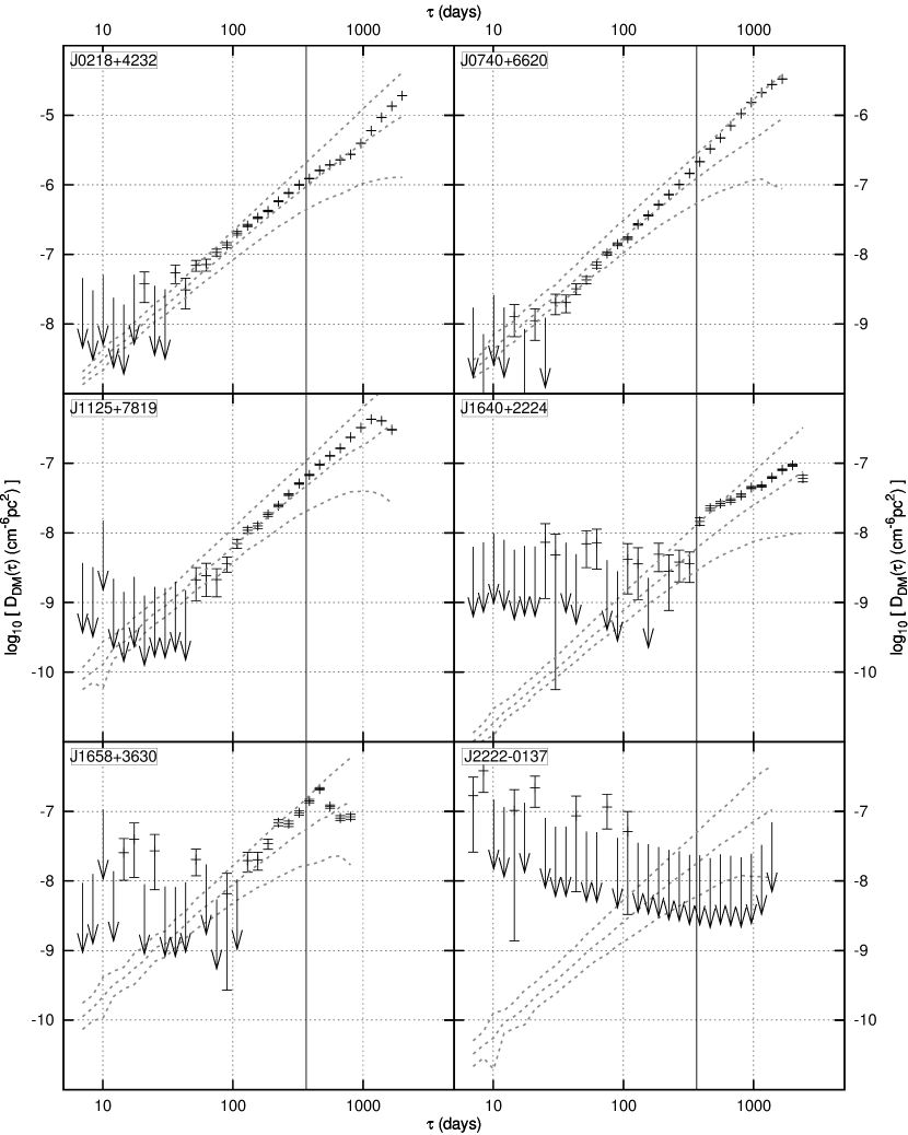
Figure 5: Structure functions for the DM time series presented in Fig. 2. The dashed lines indicate the median and 68% confidence interval of the Kolmogorov structure function simulations (see text for details). The solid black vertical line indicates $\tau=1\,\text{yr}$. The white noise level has been subtracted from the data and the Kolmogorov model. Arrows indicate upper limits for measurements consistent with zero at the 1-$\sigma$ level.

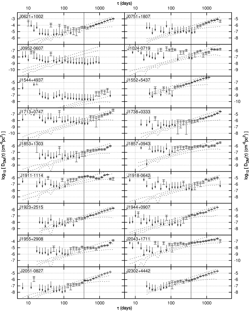
Figure 6: Same as Fig. 5, but for the DM time series presented in Fig. 3.

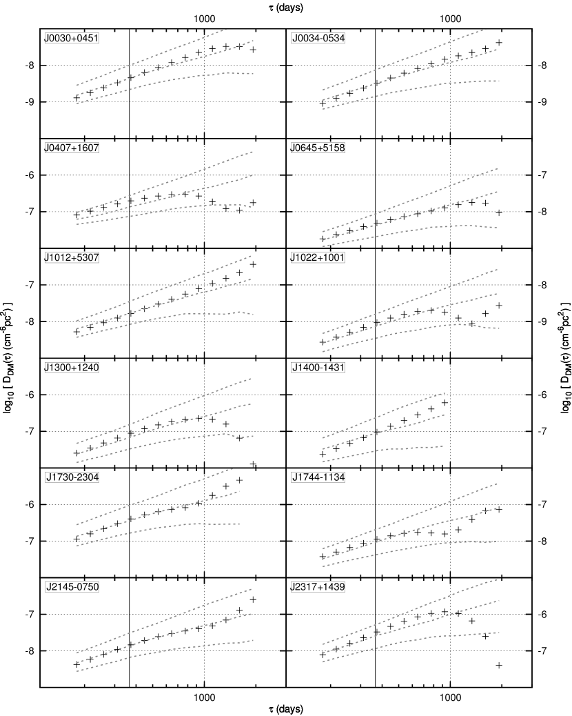
Figure 7: Structure functions for the DM time series presented in Fig. 1 after mitigation of the Solar wind signal. The representation is the same as in Fig. 5.

4.4 Comparison to PTA results

As the mitigation of the IISM is an important consideration in PTA gravitational-wave analysis, DM time series of PTA pulsars are studied extensively (e.g. Keith et al. 2013; Desvignes et al. 2016; Jones et al. 2017), although these use much lower cadence and are obtained at much higher frequencies (typically $\sim$300-2000 MHz). The published PTA DM time series present datasets that mostly end around the start of our dataset, making a direct comparison of the DM time series difficult.

Keith et al. (2013) used observations from three frequency bands centred at $\sim$700 MHz, $\sim$1400 MHz and $\sim$3100 MHz. From these data, they derived one DM estimate every three months for the 20 pulsars in their sample. As this work used the Parkes Pulsar Timing Array (PPTA) observations from the Parkes telescope (which is located in the southern hemisphere), there are only seven pulsars from their study that we also observed – all of which are at a low declination where the sensitivity of LOFAR decreases dramatically (e.g. Noutsos et al. 2015). Keith et al. (2013) do not see clear deviations from the simple symmetric Solar wind model they applied, but this is expected as their DM precision is not high enough. However, for some pulsars (e.g. PSR J1857+0943), their DM precision is comparable to the one achieved with LOFAR. Keith et al. (2013) also give the value of the structure function at a time lag of 1000 days, which is consistent with our results within the red-noise uncertainty.

Desvignes et al. (2016) present timing results for 42 MSPs observed with telescopes of the European Pulsar Timing Array (EPTA). The observations were taken across a range of frequencies between 350 MHz and 2.6 GHz, with the majority being taken around 1.4 GHz. Of the pulsars in their study, 20 are in common with this work. In their paper, they do not present DM time series, but instead used the temponest software to model the DM variations as a second-order polynomial plus a spectral noise model. This makes a comparison of individual measurements difficult, but the large-scale trends can be compared. Whether or not the LOFAR data provide more information on the DM variability is again strongly pulsar dependent. For example, we detect a very clear DM signal in PSR J2317+1439 (see Fig. 1) while Desvignes et al. (2016) only find a DM trend at the $1\sigma$-level, consistent with the overall trend we see in the early part of our dataset.

Jones et al. (2017) present data from the North American Nanohertz Observatory for Gravitational Waves (NANOGrav) collaboration, analysing the DM time evolution of 37 MSPs at frequencies between 300 MHz and 2.4 GHz, 18 of which we analysed in this study. Again, the question of which instrument provides greater precision in DM measurements is pulsar dependent: LOFAR provides a much higher precision for PSR J1012+5307, whereas the higher-frequency NANOGrav data provide a much higher precision for PSR J1857+0943 (PSR B1855+09 in Jones et al. 2017).

Overall, we find no inconsistency between our results and the highlighted recent PTA publications. However, this is partly caused by the fact that the datasets are difficult to compare due to a lack of overlap in observing epochs, and differences in data representation.

4.5 Consequences for PTAs

In pulsar timing experiments, the actual ToA is usually not the measure of interest. Instead, the DM-corrected, infinite-frequency ToA $T_{\infty}$ is the relevant measure when trying to measure IISM-independent effects. As variations in the DM at a relevant magnitude are very common, they usually have to be accounted for (Verbiest et al. 2016). In the following, we will discuss different approaches to apply corrections of the dispersive delays to ToAs at 1.4 GHz, with a timing precision of $\sigma_{\text{ToA}}=\text{$1\text{\,}\mathrm{\SIUnitSymbolMicro s}$}$.

There are two basic approaches to consider. Approach I would be to calculate the in-band DM (as in this paper) and apply the according dispersive delay (using Eq. 1) to the timing ToAs. The uncertainty on $T_{\infty}$ would then be

$$\sigma_{\infty}=\sqrt{\sigma_{\text{ToA}}^{2}+\sigma_{\text{disp}}^{2}}.$$ (6)

To avoid the dispersive correction of being the dominant factor in this example ($\sigma_{\text{ToA}}=\text{$1\text{\,}\mathrm{\SIUnitSymbolMicro s}$}$ at 1.4 GHz), the uncertainty on the DM would have to be lower than $5\times 10^{-4}$ cm^-3 pc, which would not be achievable from in-band measurements at 1.4 GHz with a bandwidth of $\sim$300 MHz, but potentially from simultaneous lower-frequency DM measurements as presented in this paper. Additionally, high-cadence DM time series could be smoothed to increase the precision of the dispersive corrections if the DM variations are smooth.

Approach II would be to use ToAs from multiple frequency bands and fit for the DM and $T_{\infty}$ simultaneously. This has the advantage of using the entire available bandwidth, but the disadvantage that exactly simultaneous observations may not be available, in which case short-term signatures from any timing parameter (e.g. parameters describing the binary motion) have to be ruled out. Also, non-simultaneous observations can have a significantly different DM if they are too far separated in time (see Lam et al. 2015).

Lee et al. (2014) investigated how the choice of the observing frequencies $\nu_{i}$ and the corresponding ToA uncertainties $\sigma_{i}$ affect the precision of the infinite-frequency ToAs. Equation 12 of their paper shows this relation in the case of only two observing frequencies:

$$\left<\delta T_{\infty}^{2}\right>=\frac{\sigma_{1}^{2}\nu_{1}^{4}+\sigma_{2}^{2}\nu_{2}^{4}}{(\nu_{1}^{2}-\nu_{2}^{2})^{2}}.$$ (7)

The $\sigma_{\infty}$ can be computed as the square root of the above expression. While the special case of only two ToAs is simplified, the general conclusions also hold for cases with additional observing frequencies. Most importantly, the frequency band with the largest $Q=\sigma^{2}\nu^{4}$ dominates the uncertainty in $T_{\infty}$. Due to the strong frequency dependence of $Q$, the highest frequency has to be the most-precisely measured in order to benefit from the additional bandwidth. If $\nu_{1}$ is our most precise timing frequency and observations at $\nu_{1}$ and $\nu_{2}$ are used to calculate $T_{\infty}$ ($\sigma_{2}>\sigma_{1}$), Fig. 8 illustrates that $\nu_{2}$ should be smaller than $\nu_{1}$ to achieve a timing precision close to $\sigma_{1}$. If $\nu_{2}$ is the higher frequency, $\sigma_{\infty}$ is limited by $\sigma_{2}$. In PTA data, the smallest ToA uncertainty is often obtained at 1.4 GHz, so observations at lower frequencies should be used to correct for DM variability. In the case of the LOFAR observations presented in this paper, a frequency-integrated ToA uncertainty of $\sim$$100\text{\,}\mathrm{\SIUnitSymbolMicro s}$ or better would be required to not dominate DM corrections at the $1\text{\,}\mathrm{\SIUnitSymbolMicro s}$-level. This condition is fulfilled for all pulsars in our sample except for PSR J0621+1001 (see Table 1), which is a pulsar that is usually timed at an RMS much worse than $1\text{\,}\mathrm{\SIUnitSymbolMicro s}$ (see e.g. Desvignes et al. 2016). This shows that Approach II should be preferred over Approach I, if it is applicable.

Figure 8: Illustration of Eq. 7 (Eq. 12 in Lee et al. 2014) for an observation at two frequency bands. The uncertainty of the infinite-frequency ToA is plotted as a function of $\nu_{2}$, with $\nu_{2}$ providing less precise ToAs than $\nu_{1}$ ($\sigma_{2}=5.0\sigma_{1}$). All quantities are given relative to the frequency and ToA uncertainty of Band 1. On the left side of the plot ($\nu_{2}\ll\nu_{1}$), $\sigma_{\infty}$ approaches $\sigma_{1}$, whereas on the right side ($\nu_{2}\gg\nu_{1}$) it approaches $\sigma_{2}$. This shows that the precision of the higher-frequency band is the limiting factor on the precision of the infinite-frequency ToA.

To illustrate the superiority of Approach II over Approach I, we will go through an example of correcting for the dispersive delay in 1.4 GHz observations using LOFAR. We assume $\nu_{1}=1.4\,\text{GHz}$, $\sigma_{1}=\text{$1\text{\,}\mathrm{\SIUnitSymbolMicro s}$}$, $\nu_{2}=150\,\text{MHz}$ and $\sigma_{2}=\text{$100\text{\,}\mathrm{\SIUnitSymbolMicro s}$}$. We note that a ToA precision of $100\text{\,}\mathrm{\SIUnitSymbolMicro s}$ is a worst-case scenario. Using Approach II, we get $\sigma_{\infty}=\text{$1.5\text{\,}\mathrm{\SIUnitSymbolMicro s}$}$. For Approach I, we assume ten ToAs around $\nu_{2}$ across a bandwidth of 75 MHz, each with an uncertainty of $\sqrt{10}\times\text{$100\text{\,}\mathrm{\SIUnitSymbolMicro s}$}$ and use Eq. 10 of Lee et al. (2014) to compute the DM uncertainty. The resulting $\sigma_{\infty}$ is $3.8\text{\,}\mathrm{\SIUnitSymbolMicro s}$, which is worse by a factor of 2.5.

A major caveat of using LOFAR observations for DM corrections at higher frequencies lies in the spectra of pulsars: Pulsars with steep spectra are bright at low frequencies and allow for highly precise DM corrections, but are fainter at high frequencies, such that the timing precision may be so low that DM corrections are less relevant. On the other hand, pulsars with flatter spectra tend to have a high ToA precision at high frequencies, but are very faint at low frequencies due to the steep spectral index of the sky background noise, which is of order 2.5 (Lawson et al. 1987). For example, the pulsar with the best DM precision in our sample is PSR J0034$-$0534, but its timing RMS at 1.4 GHz is only average ($4.27\text{\,}\mathrm{\SIUnitSymbolMicro s}$, see Perera et al. 2019). The well-timed PSR J1713+0747, however, is so faint we cannot even detect it in GLOW data and achieve a DM precision an order of magnitude worse than for PSR J0034$-$0534.

It therefore follows that Approach I using LOFAR data would currently not improve the PTA timing precision for most sources, which could be solved by increasing the timing precision of steep-spectrum sources at 1.4 GHz or improving the DM precision of flat-spectrum sources at low frequencies. The latter could be achieved by greatly increasing the integration time with the LOFAR Core or using more sensitive telescopes like the upcoming Square Kilometre Array phase-one low-frequency bands (SKA1-LOW; e.g.  Janssen et al. 2015). Using a slightly higher frequency might also help if the spectrum of the pulsar is very flat – the optimal frequency for the DM measurement is strongly pulsar dependent. As the timing precision of steep-spectrum PTA sources continues to increase due to improved telescopes, the significance of highly precise DM time series such as those presented in this work will become crucial for DM corrections. However, Approach II should already now improve the timing precision of PTAs for many sources, as it provides more precise corrections for the dispersive delays. We reserve such an analysis for a future paper, however.

4.6 Data access

Our ToAs, timing models, templates and DM time series are available online on Zenodo. The raw observations taken with the LOFAR Core can be accessed via the LOFAR Long Term Archive. The raw GLOW data are available upon request.

5 Conclusions

We present low-frequency DM time series for 36 MSPs over up to 7.1 years, obtained from observations with the LOFAR Core and the individual GLOW telescopes. Except for the pulsars with very high DM uncertainty (i.e. greater than $\sim 10^{-4}$ cm^-3 pc), all pulsars show significant variations in DM. Twelve pulsars show a clear Solar wind signal in their DM time series that can usually not be modelled by a spherically symmetric electron content with constant amplitude, which is often used in pulsar timing. All of the IISM-related DM variations we present are consistent with a Kolmogorov turbulence spectrum.

Acknowledging the caveat that LOFAR often provides a high DM precision for pulsars that are poorly timed at higher frequencies, and vice versa, we show that our LOFAR DM monitoring could be used to correct variations of the dispersive delays in higher-frequency observations from PTAs. We do not find evidence for a frequency-dependent DM, so we expect the impact of this effect to be limited.