Bose-Einstein momentum correlations at fixed multiplicities: Lessons from an exactly solvable thermal model for $pp$ collisions at the LHC

Abstract

Two-particle momentum correlations of $N$ identical bosons are studied in the quantum canonical ensemble. We define the latter as a properly selected subensemble of events associated with the grand canonical ensemble which is characterized by a constant temperature and a harmonic-trap chemical potential. The merits of this toy model are that it can be solved exactly, and that it demonstrates some interesting features revealed recently in small systems created in $p+p$ collisions at the LHC. We find that partial coherence can be observed in particle emission from completely thermal ensembles of events if instead of inclusive measurements one studies the two-boson distribution functions related to the events with particle numbers selected in some fixed multiplicity bins. The corresponding coherence effects increase with the multiplicity.

I Introduction

Femtoscopic study results on the two-particle momentum correlations (see, e.g., Ref. Sin-1 ) in $p+p$ collisions at the CERN Large Hadron Collider (LHC) have been presented recently by the ALICE Alice , ATLAS Atlas , CMS CMS , and LHCb LHCb Collaborations. It was found that the femtoscopic radii measured by the ATLAS and CMS Collaborations decrease with the increasing momentum of a pair. It can be interpreted in the hydrodynamical approach as the decrease of “homogeneity lengths ” Sin-2 (sizes of the effective emission region) due to generation by the collective flow $x-p$ correlations. Also, one found that the “correlation strength” parameter $\lambda$ is essentially less than unity. This is at variance with the expected behavior for emission from thermalized systems Sin-1 .

Another very interesting observation is the saturation of the multiplicity dependence of the interferometry correlation radius parameters for very high charged-particle multiplicity. Such an effect was observed recently by the ATLAS Atlas and CMS CMS Collaborations. Then, while there is some evidence that hydrodynamics can be successfully applied to describe particle momentum spectra in high-multiplicity $p+p$ collisions (for recent review see, e.g., Ref. Hydro-pp-1 ), it is still unclear whether the reported results on Bose-Einstein momentum correlations can be attributed to hydrodynamic evolution like in $A+A$ collisions.

In our opinion, observed peculiarities of Bose-Einstein momentum correlations in high-multiplicity $p+p$ collisions do not indicate inapplicability of hydrodynamics but can be partly associated with quantum coherence effects in small systems, when the effective system size is comparable with typical wavelength of the thermal bosons. Recall that the effective geometrical size is associated with the length of homogeneity in the system Sin-2 .

Recently, a detail analysis of inclusive spectra and Bose-Einstein correlations in small thermal quantum systems was done for the analytically solved model in Ref. Sin-0 . It is shown that if one deals (even locally) with a grand canonical ensemble, a nontrivial coherence parameter appears in inclusive two-boson spectra only in the case of coherent condensate formation. Without the latter, no coherence-induced suppression of the inclusive correlation function is possible because of the thermal Wick’s theorem.

As for nonthermal or quasithermal emission with fixed particle multiplicity, the traditional pair-correlation function is distorted for events with high phase-space density, in particular, suppression of the Bose-Einstein correlations arises. The special algorithms for symmetrization of multiboson $N$-particle states with independent particle emissions, and subsequent calculations of one- and two-particle spectra were developed in Refs. Zajc ; Pratt ; Zhang ; Urs ; Ledn ; Heinz . The situation, when particle radiation from different source points are not independent because the wave packets of emitted bosons are overlapping, was considered in Ref. Shap .

Coming back to the thermal sources, in Ref. Akk-2 the coherence effects in Bose-Einstein correlation functions in thermal systems are studied in subensembles of events with fixed multiplicities. The analytical calculations were done in the corresponding canonical ensemble. It was found that the correlation functions are suppressed in a finite system in a large volume and low particle number density approximation. In the present paper, we study the two-boson momentum correlations in small systems with high particle number densities at the moment when the system breaks up. Such almost sudden freeze-out can happen due to very fast expansion (when the homogeneity lengths are around $1$ fm) of the matter formed in high-multiplicity $p+p$ collisions at the LHC. To make the problem tractable we utilize a model of the finite system with smooth edges to avoid strong boundary effects. Keeping in mind the collective expansion inherent to systems created in particle and nucleus collisions, one can associate the corresponding system’s scale-parameter with the homogeneity length.

The particle momentum spectra at a sharp freeze-out are formed according to Ref. Cooper , which is a reasonable approximation for $p+p$ collisions. In order to keep things as simple as possible, we consider nonrelativistic ideal gas of bosons at fixed temperature trapped by means of a harmonic chemical potential. Such an exactly solvable toy model of inhomogeneous and finite-sized systems is mathematically identical to an ideal bosonic gas trapped by a harmonic potential. Then we apply the fixed particle number constraint to the corresponding grand-canonical statistical operator and discuss the influence of such constraints on one-particle momentum spectra and two-boson momentum correlations.

II Ideal gas of bosons in a harmonic trap with fixed particle number constraint

We begin with a brief overview of the properties of the grand-canonical ensemble of noninteracting nonrelativistic quantum-field bosons at fixed temperature, $T$, trapped by a harmonic chemical potential. For such a quantum field the Hamiltonian is given by

$$H=\int d^{3}r\Psi^{{\dagger}}(\textbf{r})\left(-\frac{1}{2m}\nabla^{2}\right)\Psi(\textbf{r}),$$ (1)

where the operators $\Psi^{{\dagger}}(\textbf{r})$ and $\Psi(\textbf{r})$ are the creation and annihilation operators, respectively. They fulfill the commutation relations

$$[\Psi(\textbf{r}),\Psi^{{\dagger}}(\textbf{r}^{\prime})]=\delta^{(3)}(\textbf{r}-\textbf{r}^{\prime}),$$ (2)

and

$$[\Psi(\textbf{r}),\Psi(\textbf{r}^{\prime})]=[\Psi^{{\dagger}}(\textbf{r}),\Psi^{{\dagger}}(\textbf{r}^{\prime})]=0.$$ (3)

The Fourier transformed operators are defined as

$$\Psi(\textbf{p})=(2\pi)^{-3/2}\int d^{3}re^{-i\textbf{p}\textbf{r}}\Psi(\textbf{r}),$$ (4)

$$\Psi^{{\dagger}}(\textbf{p})=(2\pi)^{-3/2}\int d^{3}re^{i\textbf{p}\textbf{r}}\Psi^{{\dagger}}(\textbf{r}).$$ (5)

They satisfy the following canonical commutation relations:

$$[\Psi(\textbf{p}),\Psi^{{\dagger}}(\textbf{p}^{\prime})]=\delta^{(3)}(\textbf{p}-\textbf{p}^{\prime}),$$ (6)

and

$$[\Psi(\textbf{p}),\Psi(\textbf{p}^{\prime})]=[\Psi^{{\dagger}}(\textbf{p}),\Psi^{{\dagger}}(\textbf{p}^{\prime})]=0.$$ (7)

The grand-canonical ensemble of such a system can be represented by the thermal statistical operator $\rho$,

$$\rho=\frac{1}{Z}\hat{\rho},$$ (8)

where $Z$ is the grand-canonical partition function,

$$Z=Tr[\hat{\rho}],$$ (9)

and

$$\hat{\rho}=e^{-\beta\widehat{H}},$$ (10)

$$\widehat{H}=\int d^{3}r\Psi^{{\dagger}}(\textbf{r})\left(-\frac{1}{2m}\nabla^{2}-\mu(\textbf{r})\right)\Psi(\textbf{r}),$$ (11)

where $\beta=1/T$ is inverse temperature. The chemical potential, $\mu(\textbf{r})$, reads

$$\mu(\textbf{r})=-\frac{m}{2}(\omega_{x}^{2}x^{2}+\omega_{y}^{2}y^{2}+\omega_{z}^{2}z^{2})+\hat{\mu},$$ (12)

where $\hat{\mu}=\mbox{const}$. The expectation value of an operator $O$ can be expressed as

$$\langle O\rangle=Tr[\rho O].$$ (13)

It is well known that $\widehat{H}$ is not diagonal in momentum (plane-wave) representation but can be diagonalized in the oscillator representation. Decomposing $\Psi(\textbf{r})$ and $\Psi^{{\dagger}}(\textbf{r})$ in terms of the harmonic oscillator eigenfunctions we get

$$\Psi(\textbf{r})=\sum_{n,k,l=0}^{\infty}\alpha(n,k,l)\phi_{n}(x)\phi_{k}(y)\phi_{l}(z),$$ (14)

where the creation, $\alpha^{{\dagger}}(n,k,l)$, and annihilation, $\alpha(n,k,l)$, operators satisfy the commutation relations

$$[\alpha(n,k,l),\alpha^{{\dagger}}(n^{\prime},k^{\prime},l^{\prime})]=\delta_{nn^{\prime}}\delta_{kk^{\prime}}\delta_{ll^{\prime}},$$ (15)

and

$$[\alpha(n,k,l),\alpha(n^{\prime},k^{\prime},l^{\prime})]=[\alpha^{{\dagger}}(n,k,l),\alpha^{{\dagger}}(n^{\prime},k^{\prime},l^{\prime})]=0.$$ (16)

Functions $\phi_{n}(x)$, $\phi_{k}(y)$, $\phi_{l}(z)$ are the harmonic oscillator eigenfunctions satisfying corresponding equations, e.g.,

$$\left(\frac{d^{2}}{dx^{2}}-m\omega_{x}^{2}x^{2}+2m\epsilon_{n}\right)\phi_{n}(x)=0.$$ (17)

The normalized solution of Eq. (17) reads

$$\phi_{n}(x)=(2^{n}n!\pi^{1/2}b_{x})^{-1/2}H_{n}\left(\frac{x}{b_{x}}\right)\exp\left(-\frac{1}{2}\left(\frac{x}{b_{x}}\right)^{2}\right),$$ (18)

where $H_{n}(x/b_{x})$ is the Hermite polynomial, and

$$\epsilon_{n}=\omega_{x}\left(n+\frac{1}{2}\right),$$ (19)

$$b_{x}=(m\omega_{x})^{-1/2}.$$ (20)

Eigenfunctions (18) are complete,

$$\sum_{n=0}^{\infty}\phi_{n}(x)\phi_{n}^{*}(x^{\prime})=\delta(x-x^{\prime}),$$ (21)

and orthonormal

$$\int_{-\infty}^{\infty}\phi_{n}(x)\phi_{n^{\prime}}^{*}(x)dx=\delta_{nn^{\prime}}.$$ (22)

Then, from Eq. (14) it immediately follows that

$$\alpha(n,k,l)=\int_{-\infty}^{\infty}dxdydz\phi_{n}^{*}(x)\phi_{k}^{*}(y)\phi_{l}^{*}(z)\Psi(\textbf{r}).$$ (23)

In such a basis the $\widehat{H}$ reads

$$\widehat{H}=\sum_{n,k,l=0}^{\infty}(\epsilon_{n}+\epsilon_{k}+\epsilon_{l}-\widehat{\mu})\alpha^{{\dagger}}(n,k,l)\alpha(n,k,l).$$ (24)

Equation (24) allows one to calculate expectation values (13) for products of $\alpha^{{\dagger}}$ and $\alpha$ operators. It can be done in various ways. It is more appropriate here to use the method which was used to prove the Wick’s theorem for the grand-canonical ensemble (see, e.g., Ref. Wick ) as the extension of it can be used for the case of the canonical ensemble. First, using the eigenstates

$$|\textbf{j}_{1},...,\textbf{j}_{N}\rangle=\frac{1}{\sqrt{N!}}\alpha^{{\dagger}}(\textbf{j}_{1})...\alpha^{{\dagger}}(\textbf{j}_{N})|0\rangle$$ (25)

of the particle number operator $\sum_{\textbf{j}}\alpha^{{\dagger}}(\textbf{j})\alpha(\textbf{j})$, and the identity

$$\sum_{N=0}^{\infty}\sum_{\textbf{j}_{1}=\textbf{0}}^{\infty}...\sum_{\textbf{j}_{N}=\textbf{0}}^{{\infty}}|\textbf{j}_{1},...,\textbf{j}_{N}\rangle\langle\textbf{j}_{1},...,\textbf{j}_{N}|=1,$$ (26)

which express the completeness and normalization of this basis, one can insert Eq. (24) into Eq. (10) and write $\hat{\rho}$ in the harmonic oscillator basis,

$$\hat{\rho}=\sum_{N}\sum_{\textbf{j}_{1}}...\sum_{\textbf{j}_{N}}e^{-\beta(\epsilon_{\textbf{j}_{1}}-\hat{\mu})}...e^{-\beta(\epsilon_{\textbf{j}_{N}}-\hat{\mu})}|\textbf{j}_{1},...,\textbf{j}_{N}\rangle\langle\textbf{j}_{1},...,\textbf{j}_{N}|.$$ (27)

We denote here

$$\epsilon_{\textbf{j}}=\epsilon_{n,k,l}=\epsilon_{n}+\epsilon_{k}+\epsilon_{l}=\omega_{x}\left(n+\frac{1}{2}\right)+\omega_{y}\left(k+\frac{1}{2}\right)+\omega_{z}\left(l+\frac{1}{2}\right).$$ (28)

Then, using an elementary operator algebra and Eq. (27) one can see that

$$\alpha(\textbf{j})\hat{\rho}=\hat{\rho}\alpha(\textbf{j})e^{-\beta(\epsilon_{\textbf{j}}-\hat{\mu})}.$$ (29)

Using trace invariance under the cyclic permutation of an operator, we get

$$Tr[\hat{\rho}\alpha^{{\dagger}}(\textbf{j}_{1})\alpha(\textbf{j}_{2})]=$$

$$e^{-\beta(\epsilon_{\textbf{j}_{2}}-\hat{\mu})}Tr[\hat{\rho}\alpha(\textbf{j}_{2})\alpha^{{\dagger}}(\textbf{j}_{1})]=e^{-\beta(\epsilon_{\textbf{j}_{2}}-\hat{\mu})}(Tr[\hat{\rho}\alpha^{{\dagger}}(\textbf{j}_{1})\alpha(\textbf{j}_{2})]+\delta_{\textbf{j}_{1}\textbf{j}_{2}}Tr[\hat{\rho}]).$$ (30)

The Kronecker delta in the above equation, $\delta_{\textbf{j}_{1}\textbf{j}_{2}}$, is

$$\delta_{\textbf{j}_{1}\textbf{j}_{2}}=\delta_{n_{1}n_{2}}\delta_{k_{1}k_{2}}\delta_{l_{1}l_{2}}.$$ (31)

From Eq. (30) we have

$$\langle\alpha^{{\dagger}}(\textbf{j}_{1})\alpha(\textbf{j}_{2})\rangle=\frac{1}{Tr[\hat{\rho}]}Tr[\hat{\rho}\alpha^{{\dagger}}(\textbf{j}_{1})\alpha(\textbf{j}_{2})]=\frac{\delta_{\textbf{j}_{1}\textbf{j}_{2}}}{e^{\beta(\epsilon_{\textbf{j}_{2}}-\hat{\mu})}-1},$$ (32)

which is a familiar Bose-Einstein distribution. It follows then that

$$\langle N\rangle=\sum_{\textbf{j}}\langle\alpha^{{\dagger}}(\textbf{j})\alpha(\textbf{j})\rangle.$$ (33)

In a similar way, one can get

$$Tr[\hat{\rho}\alpha^{{\dagger}}(\textbf{j}_{1})\alpha^{{\dagger}}(\textbf{j}_{2})\alpha(\textbf{j}_{3})\alpha(\textbf{j}_{4})]=$$

$$e^{-\beta(\epsilon_{\textbf{j}_{4}}-\hat{\mu})}(\delta_{\textbf{j}_{1}\textbf{j}_{4}}Tr[\hat{\rho}\alpha^{{\dagger}}(\textbf{j}_{2})\alpha(\textbf{j}_{3})]+\delta_{\textbf{j}_{2}\textbf{j}_{4}}Tr[\hat{\rho}\alpha^{{\dagger}}(\textbf{j}_{1})\alpha(\textbf{j}_{3})]+Tr[\hat{\rho}\alpha^{{\dagger}}(\textbf{j}_{1})\alpha^{{\dagger}}(\textbf{j}_{2})\alpha(\textbf{j}_{3})\alpha(\textbf{j}_{4})]),$$ (34)

Then, taking into account Eq. (32) we have

$$\langle\alpha^{{\dagger}}(\textbf{j}_{1})\alpha^{{\dagger}}(\textbf{j}_{2})\alpha(\textbf{j}_{3})\alpha(\textbf{j}_{4})\rangle=$$

$$\langle\alpha^{{\dagger}}(\textbf{j}_{2})\alpha(\textbf{j}_{3})\rangle\langle\alpha^{{\dagger}}(\textbf{j}_{1})\alpha(\textbf{j}_{4})\rangle+\langle\alpha^{{\dagger}}(\textbf{j}_{1})\alpha(\textbf{j}_{3})\rangle\langle\alpha^{{\dagger}}(\textbf{j}_{2})\alpha(\textbf{j}_{4})\rangle,$$ (35)

which is nothing but the particular case of the thermal Wick’s theorem. Then, utilizing Eq. (14) and Eqs. (32) and (35) one can calculate expectation values of $\Psi$ and $\Psi^{{\dagger}}$ operators.

Now, let us apply the fixed particle number constraint to the grand-canonical statistical operator (8) to define canonical statistical operator $\rho_{N}$. For this aim, one can utilize the projection operator ${\cal P}_{N}$,

$${\cal P}_{N}=\frac{1}{N!}\int d^{3}r_{1}...d^{3}r_{N}\Psi^{{\dagger}}(\textbf{r}_{1})...\Psi^{{\dagger}}(\textbf{r}_{N})|0\rangle\langle 0|\Psi(\textbf{r}_{1})...\Psi(\textbf{r}_{N}),$$ (36)

which automatically invokes the corresponding constraint. Using Eqs. (14), (22) and (25) one can see that

$${\cal P}_{N}=\sum_{\textbf{j}_{1}}...\sum_{\textbf{j}_{N}}|\textbf{j}_{1},...,\textbf{j}_{N}\rangle\langle\textbf{j}_{1},...,\textbf{j}_{N}|.$$ (37)

It is worth noting that such a projection is accompanied by the proper normalization in order to insure the probability interpretation of the ensemble obtained in result of this projection. Then, using (37) we assert that the canonical statistical operator is

$$\rho_{N}=\frac{1}{Z_{N}}\hat{\rho}_{N},$$ (38)

where

$$\hat{\rho}_{N}={\cal P}_{N}\hat{\rho}{\cal P}_{N}=\sum_{\textbf{j}_{1}}...\sum_{\textbf{j}_{N}}e^{-\beta(\epsilon_{\textbf{j}_{1}}-\hat{\mu})}...e^{-\beta(\epsilon_{\textbf{j}_{N}}-\hat{\mu})}|\textbf{j}_{1},...,\textbf{j}_{N}\rangle\langle\textbf{j}_{1},...,\textbf{j}_{N}|,$$ (39)

and $Z_{N}$ is the corresponding canonical partition function,

$$Z_{N}=Tr[\hat{\rho}_{N}].$$ (40)

It follows from Eq. (39) that

$$Z=\sum_{N=0}^{\infty}Z_{N}.$$ (41)

The vacuum state, $N=0$, yields $Z_{0}=\langle 0|0\rangle=1$. Let us denote $\hat{\rho}_{N}$ associated with $\hat{\mu}=0$ as $\hat{\rho}_{N}^{0}$. Then one can readily see that $\widehat{\rho}_{N}=e^{\beta\widehat{\mu}N}\hat{\rho}_{N}^{0}$ and

$$Z_{N}=e^{\beta\hat{\mu}N}Z_{N}^{0}.$$ (42)

Therefore [see Eq. (38)] $e^{\beta\hat{\mu}N}$ is factored out and $\rho_{N}$ does not depend on $\hat{\mu}$:

$$\rho_{N}=\frac{1}{Z_{N}^{0}}\hat{\rho}_{N}^{0}.$$ (43)

The expectation value of an operator $O$ is defined as

$$\langle O\rangle_{N}=Tr[\rho_{N}O].$$ (44)

It follows from Eqs. (39) and (44) that

$$\langle O\rangle=\sum_{N=0}^{\infty}\frac{Z_{N}}{Z}\langle O\rangle_{N}.$$ (45)

To evaluate the expectation values of operators $\alpha^{{\dagger}}(\textbf{j}_{1})\alpha(\textbf{j}_{2})$ and $\alpha^{{\dagger}}(\textbf{j}_{1})\alpha^{{\dagger}}(\textbf{j}_{2})\alpha(\textbf{j}_{3})\alpha(\textbf{j}_{4})$ with the canonical statistical operator $\rho_{N}$, one can adopt the procedure which was used above to calculate expectation values with the grand-canonical statistical operator $\rho$. It can be done in a similar way as it was done, e.g., in Ref. Akk-2 . For the reader’s convenience, below we adjust the derivation from Ref. Akk-2 for our model. A starting point is the relation

$$\alpha(\textbf{j})\hat{\rho}_{N}^{0}=\hat{\rho}_{N-1}^{0}\alpha(\textbf{j})e^{-\beta\epsilon_{\textbf{j}}}$$ (46)

which follows from Eq. (39) and commutation relations (15) and (16). Then one can exploit invariance under cyclic permutation and get the iteration equation

$$\langle\alpha^{{\dagger}}(\textbf{j}_{1})\alpha(\textbf{j}_{2})\rangle_{N}=e^{-\beta\epsilon_{\textbf{j}_{2}}}\delta_{\textbf{j}_{1}\textbf{j}_{2}}\frac{Z_{N-1}^{0}}{Z_{N}^{0}}+e^{-\beta\epsilon_{\textbf{j}_{2}}}\frac{Z_{N-1}^{0}}{Z_{N}^{0}}\langle\alpha^{{\dagger}}(\textbf{j}_{1})\alpha(\textbf{j}_{2})\rangle_{N-1}.$$ (47)

With the starting value $\langle\alpha^{{\dagger}}(\textbf{j}_{1})\alpha(\textbf{j}_{2})\rangle_{0}=0$ one can get from the above equation that

$$\langle\alpha^{{\dagger}}(\textbf{j}_{1})\alpha(\textbf{j}_{2})\rangle_{N}=\delta_{\textbf{j}_{1}\textbf{j}_{2}}\sum_{s=1}^{N}e^{-s\beta\epsilon_{\textbf{j}_{2}}}\frac{Z_{N-s}^{0}}{Z_{N}^{0}}.$$ (48)

It follows from the definition of $\rho_{N}$ [see Eqs. (38) and (39)] that

$$\sum_{\textbf{j}}\langle\alpha^{{\dagger}}(\textbf{j})\alpha(\textbf{j})\rangle_{N}=N.$$ (49)

Utilizing relation (46) we have

$$\langle\alpha^{{\dagger}}(\textbf{j}_{1})\alpha^{{\dagger}}(\textbf{j}_{2})\alpha(\textbf{j}_{3})\alpha(\textbf{j}_{4})\rangle_{N}=e^{-\beta\epsilon_{\textbf{j}_{4}}}\frac{Z_{N-1}^{0}}{Z_{N}^{0}}\langle\alpha(\textbf{j}_{4})\alpha^{{\dagger}}(\textbf{j}_{1})\alpha^{{\dagger}}(\textbf{j}_{2})\alpha(\textbf{j}_{3})\rangle_{N-1}.$$ (50)

Then the same procedure leads to

$$\langle\alpha^{{\dagger}}(\textbf{j}_{1})\alpha^{{\dagger}}(\textbf{j}_{2})\alpha(\textbf{j}_{3})\alpha(\textbf{j}_{4})\rangle_{N}=e^{-\beta\epsilon_{\textbf{j}_{4}}}\frac{Z_{N-1}^{0}}{Z_{N}^{0}}\times$$

$$\left(\langle\alpha^{{\dagger}}(\textbf{j}_{1})\alpha^{{\dagger}}(\textbf{j}_{2})\alpha(\textbf{j}_{3})\alpha(\textbf{j}_{4})\rangle_{N-1}+\delta_{\textbf{j}_{1}\textbf{j}_{4}}\langle\alpha^{{\dagger}}(\textbf{j}_{2})\alpha(\textbf{j}_{3})\rangle_{N-1}+\delta_{\textbf{j}_{2}\textbf{j}_{4}}\langle\alpha^{{\dagger}}(\textbf{j}_{1})\alpha(\textbf{j}_{3})\rangle_{N-1}\right).$$ (51)

One can show by induction that Eq. (51) can be written as

$$\langle\alpha^{{\dagger}}(\textbf{j}_{1})\alpha^{{\dagger}}(\textbf{j}_{2})\alpha(\textbf{j}_{3})\alpha(\textbf{j}_{4})\rangle_{N}=$$

$$\delta_{\textbf{j}_{1}\textbf{j}_{4}}\sum_{s=1}^{N}e^{-s\beta\epsilon_{\textbf{j}_{4}}}\frac{Z_{N-s}^{0}}{Z_{N}^{0}}\langle\alpha^{{\dagger}}(\textbf{j}_{2})\alpha(\textbf{j}_{3})\rangle_{N-s}+\delta_{\textbf{j}_{2}\textbf{j}_{4}}\sum_{s=1}^{N}e^{-s\beta\epsilon_{\textbf{j}_{4}}}\frac{Z_{N-s}^{0}}{Z_{N}^{0}}\langle\alpha^{{\dagger}}(\textbf{j}_{1})\alpha(\textbf{j}_{3})\rangle_{N-s}.$$ (52)

Then, taking into account that $\langle\alpha^{{\dagger}}(\textbf{j}_{1})\alpha(\textbf{j}_{2})\rangle_{0}=0$ and Eq. (48), we get

$$\langle\alpha^{{\dagger}}(\textbf{j}_{1})\alpha^{{\dagger}}(\textbf{j}_{2})\alpha(\textbf{j}_{3})\alpha(\textbf{j}_{4})\rangle_{N}=$$

$$(\delta_{\textbf{j}_{1}\textbf{j}_{4}}\delta_{\textbf{j}_{2}\textbf{j}_{3}}+\delta_{\textbf{j}_{1}\textbf{j}_{3}}\delta_{\textbf{j}_{2}\textbf{j}_{4}})\sum_{s=1}^{N-1}\sum_{s^{\prime}=1}^{N-s}e^{-s\beta\epsilon_{\textbf{j}_{4}}}e^{-s^{\prime}\beta\epsilon_{\textbf{j}_{3}}}\frac{Z_{N-s-s^{\prime}}^{0}}{Z_{N}^{0}}.$$ (53)

The above expressions explicitly demonstrate deviations from the Wick’s theorem in the canonical ensemble for a system of noninteracting bosons.

Canonical partition functions in Eqs. (48) and (53) can be calculated by means of the recursive formula of the canonical partition function for a system of $N$ noninteracting bosons as given in Ref. Recurr-1 (an elementary derivation of it can be seen in Ref. Akk-2 ):

$$nZ_{n}^{0}=\sum_{s=1}^{n}\sum_{\textbf{j}}e^{-s\beta\epsilon_{\textbf{j}}}Z_{n-s}^{0},$$ (54)

where $Z_{0}^{0}=\langle 0|0\rangle=1$ and $n=1,...,N$.

As a final comment we would like to point out that there is an essential difference between states defined by the grand-canonical statistical operator, $\rho$ [see Eqs. (8), (9), and (27)] and the canonical statistical operator, $\rho_{N}$ [see Eqs. (38), (39), and (40)]. While the former is a mixture of all $N$-particle states including vacuum state with $N=0$, the latter is a mixture of states with $N$ fixed to some value. In a sense, the quantum canonical state, $\rho_{N}$, can be interpreted as a state which is not completely chaotic but has some quantum coherent properties. In what follows we demonstrate that such a coherence is enhanced in the case of the Bose-Einstein condensation, when the number of particles in the ground state, $N_{0}$, is of the order of the total number of particles, $N$, and discuss possible relations of our results to two-boson momentum correlations measured in $p+p$ collisions at the LHC.

III Particle momentum spectra and correlations at fixed multiplicities

In this section we relate the model with physical observables in relativistic particle and nucleus collisions. To keep things as simple as possible, below we assume that $\omega_{x}=\omega_{y}=\omega_{z}\equiv\omega$. Note that the mean particle number, $\langle N\rangle$, defined by the grand canonical ensemble, as well as the particle number, $N$, in the canonical ensemble are the same for $\Psi$ particles and $\alpha$ quasiparticles because unitary transformation (14) does not mix creation and annihilation operators.

First, let us estimate spatial size of the system at fixed multiplicities. It is defined as $\sqrt{\frac{1}{3}\langle\textbf{r}^{2}\rangle_{N}}$, where

$$\frac{1}{3}\langle\textbf{r}^{2}\rangle_{N}=\langle x^{2}\rangle_{N}=\frac{\int dxdydzx^{2}\langle\Psi^{{\dagger}}(\textbf{r})\Psi(\textbf{r})\rangle_{N}}{\int dxdydz\langle\Psi^{{\dagger}}(\textbf{r})\Psi(\textbf{r})\rangle_{N}},$$ (55)

$\langle\Psi^{{\dagger}}(\textbf{r})\Psi(\textbf{r})\rangle_{N}$ is the mean particle number density in the canonical ensemble, and $\int dxdydz\langle\Psi^{{\dagger}}(\textbf{r})\Psi(\textbf{r})\rangle_{N}=N$. From Eqs. (14) and (48) we get

$$\langle\Psi^{{\dagger}}(\textbf{r}_{1})\Psi(\textbf{r}_{2})\rangle_{N}=$$

$$\sum_{s=1}^{N}\frac{Z_{N-s}^{0}}{Z_{N}^{0}}\sum_{n=0}^{\infty}\sum_{k=0}^{\infty}\sum_{l=0}^{\infty}\phi_{n}^{*}(x_{1})\phi_{k}^{*}(y_{1})\phi_{l}^{*}(z_{1})\phi_{n}(x_{2})\phi_{k}(y_{2})\phi_{l}(z_{2})e^{-\frac{3}{2}s\beta\omega}e^{-s\beta\omega(n+k+l)},$$ (56)

where the eigenfunctions are defined by Eq. (18), $b_{x}=b_{y}=b_{z}\equiv b$ and

$$b=(m\omega)^{-1/2},$$ (57)

see Eq. (20). Then, utilizing integral representation of the Hermite function (see e.g. Ref. math ),

$$H_{n}\left(\frac{x}{b}\right)=\left(\frac{b}{i}\right)^{n}\frac{b}{2\sqrt{\pi}}e^{\frac{x^{2}}{b^{2}}}\int_{-\infty}^{+\infty}v^{n}e^{-\frac{1}{4}b^{2}v^{2}+ixv}dv,$$ (58)

one can perform summations over $n,k,l$ in Eq. (56). A lengthy but straightforward calculation results in

$$\langle\Psi^{{\dagger}}(\textbf{r}_{1})\Psi(\textbf{r}_{2})\rangle_{N}=$$

$$\sum_{s=1}^{N}\frac{1}{(2\pi)^{3/2}}\frac{1}{b^{3}}\frac{Z_{N-s}^{0}}{Z_{N}^{0}}\left(\sinh(\beta\omega s)\right)^{-3/2}\exp\left(-\frac{\textbf{r}_{1}^{2}+\textbf{r}_{2}^{2}}{2b^{2}\tanh(\beta\omega s)}\right)\exp\left(\frac{\textbf{r}_{1}\textbf{r}_{2}}{b^{2}\sinh(\beta\omega s)}\right).$$ (59)

Utilizing identity $(\tanh A)^{-1}-(\sinh A)^{-1}=\tanh(A/2)$, we have from Eq. (59) that mean particle number density in the canonical ensemble reads

$$\langle\Psi^{{\dagger}}(\textbf{r})\Psi(\textbf{r})\rangle_{N}=\sum_{s=1}^{N}\frac{1}{(2\pi)^{3/2}}\frac{1}{b^{3}}\frac{Z_{N-s}^{0}}{Z_{N}^{0}}\left(\sinh(\beta\omega s)\right)^{-3/2}\exp\left(-\frac{\tanh(\frac{1}{2}\beta\omega s)}{b^{2}}\textbf{r}^{2}\right).$$ (60)

Substituting the above expression in Eq. (55) we readily find

$$\langle x^{2}\rangle_{N}=\frac{1}{2}b^{2}\frac{\sum_{s=1}^{N}\frac{Z_{N-s}^{0}}{Z_{N}^{0}}\left(\sinh(\beta\omega s)\right)^{-3/2}\left(\tanh(\frac{1}{2}\beta\omega s)\right)^{-5/2}}{\sum_{s=1}^{N}\frac{Z_{N-s}^{0}}{Z_{N}^{0}}\left(\sinh(\beta\omega s)\right)^{-3/2}\left(\tanh(\frac{1}{2}\beta\omega s)\right)^{-3/2}}.$$ (61)

To relate parameters of the model with physically meaningful parameters in relativistic particle and nucleus collisions, it is convenient to introduce parameter $R$ such as

$$\omega=\frac{1}{R\sqrt{\beta m}},$$ (62)

then $\frac{m\omega^{2}}{2}=\frac{1}{2\beta R^{2}}$; see Eq. (12). In what follows we treat $R$ as free parameter instead of $\omega$. As we will see below, $R$ can be approximately associated with the spatial size of the system, $\sqrt{\langle x^{2}\rangle_{N}}$.

Then

$$\beta\omega=\frac{1}{R}\sqrt{\frac{\beta}{m}}=\frac{\Lambda_{T}}{R},$$ (63)

and

$$b=\frac{1}{\sqrt{m\omega}}=\sqrt{\Lambda_{T}R},$$ (64)

where $\Lambda_{T}$ is the thermal wavelength, which we defined as

$$\Lambda_{T}=\frac{1}{\sqrt{mT}}.$$ (65)

We now turn to the two-particle momentum correlation functions. Two-particle momentum correlation function is defined as ratio of two-particle momentum spectrum to one-particle ones and can be written in canonical ensemble at fixed multiplicities as

$$C_{N}(\textbf{k},\textbf{q})=G_{N}\frac{\langle\Psi^{{\dagger}}(\textbf{p}_{1})\Psi^{{\dagger}}(\textbf{p}_{2})\Psi(\textbf{p}_{1})\Psi(\textbf{p}_{2})\rangle_{N}}{\langle\Psi^{{\dagger}}(\textbf{p}_{1})\Psi(\textbf{p}_{1})\rangle_{N}\langle\Psi^{{\dagger}}(\textbf{p}_{2})\Psi(\textbf{p}_{2})\rangle_{N}}.$$ (66)

Here ${\bf k}=({\bf p}_{1}+{\bf p}_{2})/2$, ${\bf q}={\bf p}_{2}-{\bf p}_{1}$, and $G_{N}$ is the normalization constant. The latter is needed to normalize the theoretical correlation function in accordance with normalization that is applied by experimentalists: $C^{exp}(\textbf{k},\textbf{q})\rightarrow 1$ for $|\textbf{q}|\rightarrow\infty$.

Expressions in the denominator of Eq. (66) can be written immediately using Fourier transform of $\langle\Psi^{{\dagger}}(\textbf{r}_{1})\Psi(\textbf{r}_{2})\rangle_{N}$; see Eq. (59). We thus have

$$\langle\Psi^{{\dagger}}(\textbf{p}_{1})\Psi(\textbf{p}_{1})\rangle_{N}=\sum_{s=1}^{N}\frac{Z_{N-s}^{0}}{Z_{N}^{0}}\Phi_{1}(\textbf{k},\textbf{q},\beta\omega s),$$ (67)

$$\langle\Psi^{{\dagger}}(\textbf{p}_{2})\Psi(\textbf{p}_{2})\rangle_{N}=\sum_{s=1}^{N}\frac{Z_{N-s}^{0}}{Z_{N}^{0}}\Phi_{1}(\textbf{k},-\textbf{q},\beta\omega s),$$ (68)

where we introduced shorthand notation

$$\Phi_{1}(\textbf{k},\textbf{q},\beta\omega s)=\frac{b^{3}}{(2\pi\sinh(\beta\omega s))^{3/2}}\exp\left(-\left(\textbf{k}-\frac{1}{2}\textbf{q}\right)^{2}b^{2}\tanh(\frac{1}{2}\beta\omega s)\right).$$ (69)

Utilizing Eq. (53) and the same technique which was used to derive $\langle\Psi^{{\dagger}}(\textbf{r}_{1})\Psi(\textbf{r}_{2})\rangle_{N}$, we get after somewhat lengthy but straightforward calculations,

$$\langle\Psi^{{\dagger}}(\textbf{p}_{1})\Psi^{{\dagger}}(\textbf{p}_{2})\Psi(\textbf{p}_{1})\Psi(\textbf{p}_{2})\rangle_{N}=$$

$$\sum_{s=1}^{N-1}\sum_{s^{\prime}=1}^{N-s}\frac{Z_{N-s-s^{\prime}}^{0}}{Z_{N}^{0}}\left(\Phi_{1}(\textbf{k},\textbf{q},\beta\omega s)\Phi_{1}(\textbf{k},-\textbf{q},\beta\omega s^{\prime})+\Phi_{2}(\textbf{k},\textbf{q},\beta\omega s)\Phi_{2}(\textbf{k},-\textbf{q},\beta\omega s^{\prime})\right),$$ (70)

where we introduced notation

$$\Phi_{2}(\textbf{k},\textbf{q},\beta\omega s)=\frac{b^{3}}{(2\pi\sinh(\beta\omega s))^{3/2}}\exp\left(-\textbf{k}^{2}b^{2}\tanh(\frac{1}{2}\beta\omega s)-\textbf{q}^{2}\frac{b^{2}}{4\tanh(\frac{1}{2}\beta\omega s)}\right).$$ (71)

Inserting Eqs. (67), (68) and (70) in Eq. (66) gives us an explicit expression for the two-boson momentum correlation function at fixed multiplicities,

$$C_{N}(\textbf{k},\textbf{q})=G_{N}\frac{\sum_{s=1}^{N-1}\sum_{s^{\prime}=1}^{N-s}\frac{Z_{N-s-s^{\prime}}^{0}}{Z_{N}^{0}}\Phi_{1}(\textbf{k},\textbf{q},\beta\omega s)\Phi_{1}(\textbf{k},-\textbf{q},\beta\omega s^{\prime})}{\sum_{s=1}^{N}\frac{Z_{N-s}^{0}}{Z_{N}^{0}}\Phi_{1}(\textbf{k},\textbf{q},\beta\omega s)\sum_{s^{\prime}=1}^{N}\frac{Z_{N-s^{\prime}}^{0}}{Z_{N}^{0}}\Phi_{1}(\textbf{k},-\textbf{q},\beta\omega s^{\prime})}+$$

$$G_{N}\frac{\sum_{s=1}^{N-1}\sum_{s^{\prime}=1}^{N-s}\frac{Z_{N-s-s^{\prime}}^{0}}{Z_{N}^{0}}\Phi_{2}(\textbf{k},\textbf{q},\beta\omega s)\Phi_{2}(\textbf{k},-\textbf{q},\beta\omega s^{\prime})}{\sum_{s=1}^{N}\frac{Z_{N-s}^{0}}{Z_{N}^{0}}\Phi_{1}(\textbf{k},\textbf{q},\beta\omega s)\sum_{s^{\prime}=1}^{N}\frac{Z_{N-s^{\prime}}^{0}}{Z_{N}^{0}}\Phi_{1}(\textbf{k},-\textbf{q},\beta\omega s^{\prime})}.$$ (72)

To estimate normalization constant $G_{N}$ in Eq. (72), one needs to utilize the limit $|\textbf{q}|\rightarrow\infty$ at fixed k in the corresponding expression. One can readily see that when $|\textbf{q}|\rightarrow\infty$ at fixed k then $C_{N}(\textbf{k},\textbf{q})\rightarrow G_{N}\frac{Z_{N-2}^{0}}{Z_{N}^{0}}\left(\frac{Z^{0}_{N}}{Z^{0}_{N-1}}\right)^{2}$. It follows then that proper normalization is reached if

$$G_{N}=\frac{Z_{N}^{0}}{Z_{N-2}^{0}}\left(\frac{Z^{0}_{N-1}}{Z^{0}_{N}}\right)^{2}.$$ (73)

IV Results and discussion

In this section, we calculate one-particle momentum spectra and two-particle Bose-Einstein momentum correlations in the model. For specificity, we assume that $m$ is equal to pion mass and we take the set of parameters corresponding roughly to the values at the system’s breakup in $p+p$ collisions at the LHC energies: The temperature $T$ is set to $150$ MeV, and for $R$ we use $1.5$ and $3$ fm. The thermal wavelength $\Lambda_{T}=1/\sqrt{mT}\approx 1.36$ fm. We varied $N$ in the range $1,...,20$. Our aim here is to investigate how particle momentum spectra and correlations in the canonical ensemble with the fixed particle number constraint differ from the ones in the corresponding grand-canonical ensemble.

We start with calculations of the one-particle momentum spectra in the canonical ensemble, $n_{N}(\textbf{p})\equiv\langle\Psi^{{\dagger}}(\textbf{p})\Psi(\textbf{p})\rangle_{N}$; see Eq. (67). We compare these calculations with the ones performed in the corresponding grand-canonical ensembles where $\hat{\mu}$ were found numerically to guarantee proper values of $\langle N\rangle$, such as $\langle N\rangle=N$. One-particle momentum spectra in the grand-canonical ensembles are calculated utilizing Eq. (67) after substitution $\sum_{s=1}^{N}\frac{Z_{N-s}^{0}}{Z_{N}^{0}}\rightarrow\sum_{s=1}^{\infty}e^{\beta\hat{\mu}s}$. The results are plotted in Fig. 1 as a function of the particle momentum for several different values of the radius parameter $R$ and particle number $N$. Figure 1 demonstrates clearly that for the used range of parameter values, one-particle momentum spectra in the canonical ensembles can be approximated with good accuracy by the ones calculated in the corresponding grand-canonical ensembles.

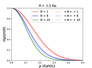
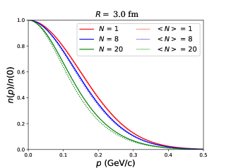
Figure 1: Normalized $n(p_{x},0,0)/n(\textbf{0})$ momentum spectra calculated in the canonical ensembles with different $N$ and $R$ (solid lines), and corresponding spectra calculated in the grand-canonical ensembles with $\langle N\rangle=N$ (dotted lines).

Figure 2 displays two-boson momentum correlation functions (72) calculated in the canonical ensembles as a function of the momentum difference. From Fig. 2 it is evident that the intercept of the correlation function, $C_{N}(\textbf{k},\textbf{0})$, is less than $2$. This can be interpreted as a result of partial coherence of particle emission Sin-1 because projection of the thermal grand-canonical ensemble into the fixed-$N$ subensemble results in the $N$-particle canonical state which is the state with partial coherence. Furthermore, one observes for small values of $R$ the essential non-Gaussianity of the correlation functions beyond the region of the correlation peak. It distinguishes two-boson correlation functions in the canonical ensembles from the ones in the corresponding grand-canonical ensembles where the correlation functions (not shown here) are well fitted by the Gaussian and intercept of the ones is equal to $2$.

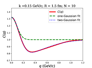
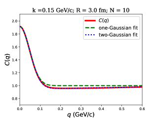
Figure 2: Correlation functions (red solid lines) and their one- and two-Gaussian fits (blue dotted and green dashed lines, respectively) with $k=0.15$ GeV/c, $N=10$, $R=1.5$ fm (left plot) and $R=3.0$ fm (right plot). See text for details.

To analyze reasons for this behavior of the correlation functions in greater detail, let us first remark that correlation function $C_{N}(\textbf{k},\textbf{q})$ [see Eqs. (72) and (73)] can be parametrized by the two-Gaussian expression

$$C_{N}^{2g}(\textbf{k},\textbf{q})=1-\lambda_{1}(\textbf{k},N)e^{-\textbf{q}^{2}R_{1}^{2}(\textbf{k},N)}+\lambda_{2}(\textbf{k},N)e^{-\textbf{q}^{2}R_{2}^{2}(\textbf{k},N)},$$ (74)

where $\lambda_{1}>0$ and $\lambda_{2}>0$. Here $1-\lambda_{1}(\textbf{k},N)e^{-\textbf{q}^{2}R_{1}^{2}(\textbf{k},N)}$ is associated with the first term in Eq. (72), and $\lambda_{2}(\textbf{k},N)e^{-\textbf{q}^{2}R_{2}^{2}(\textbf{k},N)}$ with the second one. The results of fittings are plotted in Fig. 2. It is evident that $C_{N}(\textbf{k},\textbf{q})$ is rather well fitted by Eq. (74). This suggests that much of the non-Gaussian deviations observed in Fig. 2 arises from such a two-scale structure of the correlation function. If the fitting procedure is restricted to the correlation peak region, then one observes from Fig. 2 that the correlation function is well fitted by the one-Gaussian expression

$$C_{N}^{1g}(\textbf{k},\textbf{q})=1+\lambda(\textbf{k},N)e^{-\textbf{q}^{2}R_{HBT}^{2}(\textbf{k},N)},$$ (75)

where $\lambda$ is equal to the intercept of the correlation function, $C_{N}(\textbf{k},\textbf{0})$.

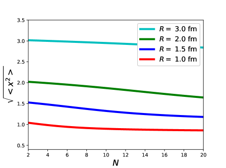
Figure 3: The $\sqrt{\langle x^{2}\rangle_{N}}$ dependence on $N$ at different $R$.

From Fig. 2 it is clear that the value of the intercept of the correlation function is strongly dependent on the value of $R$ at fixed $N$, namely, one observes that smaller values of $R$ result in smaller values of the intercept of the correlation function. The question naturally arises: why does decreasing the parameter $R$ amount to a decreasing of the intercept? Some insight into this question may be gained from Fig. 3, in which mean size of the system $\sqrt{\langle x^{2}\rangle_{N}}$ [see Eq. (61)] is plotted out to $N$. One observes from this figure that parameter $R$ roughly corresponds to the mean spatial size of the system in the varied range of $N$. It means that the decrease of $R$ at fixed $N$ results in an increase of the mean particle number density, $\varpropto N/R^{3}$.

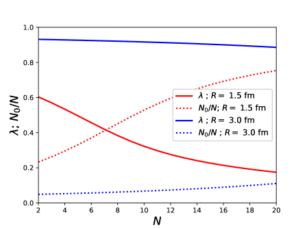
Figure 4: The $\lambda$ at $k=0.15$ GeV/c, and $N_{0}/N$ dependence on $N$ for $R=1.5$ fm and $R=3.0$ fm.

To gain further insight into these results, the $\lambda$ parameter and also the ratio of the ground-state population, $N_{0}=\langle\alpha^{{\dagger}}(\textbf{0})\alpha(\textbf{0})\rangle_{N}$ [see Eq. (48)], to the number of particles, $N$, are plotted out to $N$ in Fig. 4. It can be seen from this figure that the coherent effects, associated with the parameter $\lambda$, are significant for any $N$ if the mean size of the system is comparable to or less than the thermal wavelength $\Lambda_{T}$. One can also see from this figure that an increase of $N$ results in an increase of the value of the $N_{0}/N$ ratio and decrease of the value of the $\lambda$ parameter. To interpret this result it is instructive to compare the canonical condensate fraction, $N_{0}/N$, with its grand-canonical counterpart $\langle N_{0}\rangle/\langle N\rangle$. We start by noting that applying Cauchy’s integral formula to Eqs. (41) and (42) one can get (see, e.g., Ref. formula )

$$Z_{N}^{0}=\beta\int_{\delta-i\infty}^{\delta+i\infty}\frac{d\hat{\mu}}{2\pi i}e^{-\hat{\mu}\beta N}Z(\hat{\mu}).$$ (76)

It is well known that utilizing the above expression for approximate evaluation of the canonical partition function, in the leading order of the saddle-point approximation one obtains

$$Z_{N}^{0}\approx e^{-\hat{\mu}_{\sigma}\beta N}Z(\hat{\mu}_{\sigma}),$$ (77)

where $\hat{\mu}_{\sigma}$ is solution of the equation $\frac{d}{d\hat{\mu}}(-\hat{\mu}\beta N+\ln{Z(\hat{\mu})})=0$. For an ideal gas it means that $\hat{\mu}_{\sigma}$ is such that $\langle N\rangle=N$. Equation (77) becomes exact for $N\rightarrow\infty$. Then, using Eqs. (41), (42), and (45), one can expect that for finite but large $N$ we get $N_{0}/N\approx\langle N_{0}\rangle/\langle N\rangle$ where $\langle N_{0}\rangle/\langle N\rangle$ is the condensate fraction in the grand-canonical ensemble with $\langle N\rangle=N$. Let us compare our results for the canonical condensate fraction, $N_{0}/N$, with the grand-canonical condensate fraction for a finite mean number of particles in a three-dimensional harmonic potential BEC-1 ,

$$\frac{\langle N_{0}\rangle}{\langle N\rangle}\approx 1-\frac{\Delta}{\langle N\rangle(\beta\omega)^{3}},$$ (78)

$$\Delta=\zeta(3)+\frac{3}{2}\zeta(2)\beta\omega,$$ (79)

calculated in the approximation $\beta\omega\ll 1$. Here $\zeta(x)$ is the Riemann zeta function, $\zeta(2)\approx 1.645$ and $\zeta(3)\approx 1.202$. In the above expression we have approximated $e^{\beta(\hat{\mu}-(3/2)\omega)}\approx 1$. Identifying $\langle N\rangle$ with the actual particle number $N$, and $\beta\omega$ with $\Lambda_{T}/R$, see Eq. (63), we compare $N_{0}/N$ with $\langle N_{0}\rangle/\langle N\rangle$ in Fig. 5 for $R=1.5$ fm and $R=3$ fm.

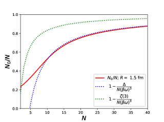
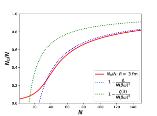
Figure 5: Canonical $N_{0}/N$ (red solid line) and its fits with Eq. (78) (blue and green dotted lines), $R=1.5$ fm (left plot), and $R=3.0$ fm (right plot). See text for details.

One observes that the approximate grand-canonical formula shows a rather good agreement with the exact canonical results even for not very large values of $N$. Loosely speaking, the canonical condensate fraction of the large system becomes noticeable (say, about $1/2$) when the mean interparticle distance, $(N/R^{3})^{-1/3}$, becomes smaller than the correlation length, for an ideal gas the latter coincides with the thermal wavelength, $\Lambda_{T}$.

While the quantitatively accurate description of the canonical condensate fraction within the grand-canonical approximation is manifest, it is not the case for fluctuations. It is well known that fluctuations in the ground state differ in the canonical and grand-canonical ensembles, and that for the latter the condensate fluctuations are very large; see, e.g., Ref. cond and references therein. In the canonical ensemble with a fixed number of particles such large fluctuations are impossible, and therefore an increase of the ground-state fraction $N_{0}/N$ increases “coherence” of the state. The latter distinguishes the ideal gas Bose-Einstein condensation in the canonical ensemble from the ideal gas Bose-Einstein condensation in the grand-canonical ensemble. It is well known that the intercept of the two-boson momentum correlation function for a maximally mixed (chaotic) state is equal to $2$, and that the one for a pure state is equal to $1$; see, e.g., Ref. Sin-1 . Therefore, an increase of the ground-state fraction, $N_{0}/N$, results in a decreasing of the $\lambda$ parameter.

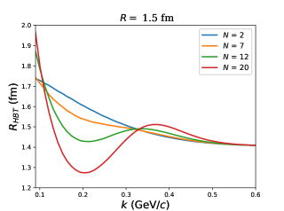
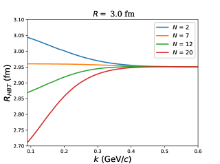
Figure 6: HBT radii obtained from the one-Gaussian fit of the two-boson correlation function in the canonical ensembles with different $N$, as a function of the pair average momentum $k$.

Finally, in Fig. 6 we plot the $R_{HBT}$ as a function of the pair momenta, $k$, for different $R$ and $N$. One observes a consistent trend: by increasing $k$ the interferometry radii, $R_{HBT}$, become independent of $N$.

V Conclusions

Usually one does not care so much about quantum coherence in the canonical ensemble at fixed multiplicities. However, utilizing the simple analytically solvable model, we demonstrated that the formulas derived in the fixed-$N$ canonical ensemble for a small inhomogeneous thermal system are not always accurately approximated by the grand-canonical ones with $\langle N\rangle=N$. Namely, we noticed that while the one-particle momentum spectra can be well approximated by the corresponding grand-canonical ensemble expressions, it is not the case for the two-boson momentum correlations. Interestingly, we observed that the most significant deviations arise if the particle number density in the canonical ensemble can increase with $N$. In the considered simple model it implies that interferometry radii are independent on $N$ at moderately high pair momenta. Then for fairly high $N$ the particle number density exceeds some limit value leading to the noticeable Bose-Einstein condensation in the corresponding ground state of the fixed-$N$ canonical ensemble state. Such a condensation strengthens the coherence properties of the canonical ensemble state, and results in the decreasing of the intercept of the two-boson momentum correlation function when $N$ increases. This may explain the observed phenomenon of partial quantum coherence in high-multiplicity $p+p$ collisions events in fixed multiplicity bins at the LHC energies Atlas ; CMS . It would be very interesting to revisit the results of experimental studies in view of our findings.

The main lesson from this study is that the canonical and grand-canonical ensembles can yield different results for two-boson momentum correlations of particles emitted by small inhomogeneous systems. The results of our analysis can be useful to elucidate the influence on the shape of the measured correlation function of both factors: an experimental selection of events with fixed multiplicity and the effects of thermalization and flow. Therefore, determination of the extent to which our results can be generalized for a realistic model of heavy ion and particle collisions could be of great interest.

References

(1) M. Gyulassy, S.K. Kauffmann, and L.W.
Wilson, Phys. Rev. C 20, 2267 (1979); M.I. Podgoretsky,
Fiz. Elem. Chast. At. Yad. 20, 628 (1989) [Sov. J. Part.
Nucl. 20, 266 (1989)]; D.H. Boal, C.-K. Gelbke, B.K.
Jennings, Rev. Mod. Phys. 62, 553 (1990); U.A. Wiedemann,
U. Heinz, Phys. Rep. 319, 145 (1999); R.M. Weiner, Phys.
Rep. 327, 249 (2000); R.M. Weiner, Introduction to
Bose-Einstein Correlations and Subatomic Interferometry (Wiley, New
York, 2000); M. Lisa, S. Pratt, R. Soltz, U. Wiedemann, Annu. Rev.
Nucl. Part. Sci. 55, 357 (2005); R. Lednický, Phys. Part.
Nuclei 40, 307 (2009) [arXiv:nucl-th/0501065].
(2) K. Aamodt et al. (ALICE Collaboration), Phys. Rev. D 84, 112004 (2011);
S. Acharya et al. (ALICE Collaboration), J. High Energy Phys. 09 (2019)
108.
(3) ATLAS Collaboration, Eur. Phys. J. C 75, 466 (2015).
(4) A.M. Sirunyan et al. (CMS Collaboration), Phys. Rev. C 97, 064912
(2018); J. High Energy Phys. 03 (2020) 014.
(5) The LHCb Collaboration, J. High Energy Phys. 12
(2017) 25.
(6) Yu.M. Sinyukov, Nucl. Phys. A 566, 589c
(1994); in: Hot Hadronic Matter: Theory and
Experiment edited by J. Letessier, H.H. Gutbrod, and J. Rafelski
(Plenum, New York, 1995), p. 309; S.V. Akkelin, Yu.M. Sinyukov,
Phys. Lett. B 356, 525 (1995); S.V. Akkelin, Yu.M.
Sinyukov, Z. Phys. C 72, 501 (1996).
(17) F. Cooper, G. Frye, Phys. Rev. D 10, 186 (1974).
(18) C. Bloch, C. De Dominicis, Nucl. Phys. 7, 459
(1958); M. Gaudin, Nucl. Phys. 15, 89 (1960);
N.N. Bogolubov, N.N. Bogolubov, Jr., An Introduction to
Quantum Statistical Mechanics (Gordon and Breach, New York, 1992);
S.R. de Groot, W.A. van Leeuwen, Ch. G. van Weert,
Relativistic Kinetic Theory (North-Holland, Amsterdam,
1980).
(19) P.T. Landsberg, Thermodynamics (Interscience, New York, 1961);
P. Borrmann and G. Franke, J. Chem. Phys. 98, 2484 (1993).
(21) I.S. Gradshteyn, I.M. Ryzhik, Table of Integrals, Series and Products
(Academic, New York, 1980).
(22) K. Huang, Statistical Mechanics (John Wiley Sons, New York, 1963);
R.M. Ziff, G.E. Uhlenbeck, and M. Kac, Phys. Rep. 32, 169 (1977).
(23) W. Ketterle, N.J. van Druten, Phys. Rev. A 54, 656 (1996).
(24) Vitaly V. Kocharovsky, Vladimir V. Kocharovsky, Martin Holthaus, C.H. Raymond Ooi,
Anatoly Svidzinsky, Wolfgang Ketterle, Marlan O. Scully,
Adv. At. Mol. Opt. Phys. 53, 291 (2006).
(25) V.M. Shapoval, P. Braun-Munzinger, Iu.A. Karpenko, Yu.M.
Sinyukov, Phys. Lett. B 725, 139 (2013).