Impacts of Noise and Structure on Quantum Information Encoded in a Quantum Memory

Abstract

As larger, higher-quality quantum devices are built and demonstrated in quantum information applications, such as quantum computation and quantum communication, the need for high-quality quantum memories to store quantum states becomes ever more pressing. Future quantum devices likely will use a variety of physical hardware, some being used primarily for processing of quantum information and others for storage. Here, we study the correlation of the structure of quantum information with physical noise models of various possible quantum memory implementations. Through numerical simulation of different noise models and approximate analytical formulas applied to a variety of interesting quantum states, we provide comparisons between quantum hardware with different structure, including both qubit- and qudit-based quantum memories. Our findings point to simple, experimentally relevant formulas for the relative lifetimes of quantum information in different quantum memories and have relevance to the design of hybrid quantum devices.

I Introduction

In many quantum information science technologies, quantum memories, which store quantum states until they are required, are an integral part of the overall architecture [1, 2]. For instance, in quantum computing applications, the ability to store a state between computations is necessary for increasing the overall fidelity of a quantum algorithm [3]. In quantum communication protocols, quantum memories make up a key part of several quantum repeater designs [4, 5]. Quantum error correction offers the ability to create an arbitrarily long-lived quantum memory, with the overhead depending on the size and complexity of the quantum hardware [6], through various protocols such as surface codes [7]. In the noisy intermediate-scale quantum (NISQ) era, however, the hardware overhead from performing quantum error correction prevents its use [8]. Nevertheless, even without error correction, today’s quantum hardware is already performing impressive demonstrations, such as quantum supremacy [9], quantum calculations in quantum chemistry [10, 11, 12], quantum simulations of many-body physics [13, 14, 15, 16, 17, 18], quantum dynamics [19, 20], quantum optimization [21, 22], quantum machine learning [23, 24], quantum internet [25, 26], and quantum networking demonstrations over long distances using satellites [27, 28], optical fibers [29, 30], and photonic quantum repeaters [31]. Going beyond these impressive, albeit small-scale, demonstrations will require high-quality quantum memories. Quantum memories can be made out of many candidate hardware platforms, including photonics [32], superconducting cavities [33], superconducting qubits [34], vacancy centers [35], trapped ions [36], and silicon quantum dots [37]. Each platform offers various benefits and drawbacks, for instance, in coherence times, fabrication difficulty, and interoperability.

Here, we study the performance of storing a variety of quantum states in various quantum memories with differing noise models, exploring the correlation of the structure of the stored quantum state with the structure of the noise model. We focus primarily on the difference of storing quantum information in qubit-based systems, where the state is stored in a possibly entangled register of qubits, to many-level qudit-based systems, where the state can be stored in one single quantum system with many levels. We provide extensive numerical calculations of such systems under amplitude damping ($T_{1}$) and dephasing ($T_{2}^{*}$) noise models, as well as simple analytic formulas for predicting the coherence requirements for the different systems and noise models to have the same memory performance. Our results point to qudit-based systems as being viable candidates for high-quality quantum memories, given the ability to engineer extremely coherent superconducting cavity systems [38, 39, 40, 41].

II Theoretical Methods

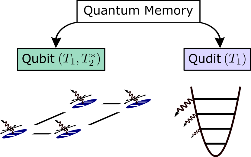
Figure 1: Quantum memories can be made out of a variety of quantum systems; here, we schematically show the noise properties of two quantum memories. Left: A quantum memory comprising qubits subject to amplitude damping (also called $T_{1}$, represented by the waves flying out of the qubits) and pure dephasing (also called $T_{2}^{*}$, denoted by the arrows pointing in many directions). Each qubit adds two noise channels, each with the same strength. Right: A quantum memory comprising a single qudit subject to amplitude damping. The noise grows as the number of levels increases.

In this section, we describe the considered noise models, how we encode quantum states, and the particular states we considered. Furthermore, to complement our numerical analysis we introduce an analytical study based on approximating the Lindblad master equation with a non-Hermitian formalism.

II.1 Noise Models

We consider the evolution of a quantum state under a noisy channel using the Lindblad master equation,

$$\frac{d\rho(t)}{dt}=\sum_{i}\gamma_{i}L(C_{i})[\rho(t)],$$ (1)

where $\rho$ is the density matrix of the system, $\gamma_{i}$ is a noise rate, $L(C_{i})[\rho(t)]=\left(C_{i}\rho(t)C_{i}^{\dagger}-\frac{1}{2}\left\{C_{i}^{\dagger}C_{i},\rho(t)\right\}\right)$ is a Lindblad superoperator, and $C_{i}$ are operators representing various noise processes. The Lindblad master equation is one of the standard approaches for studying Markovian open quantum systems [42, 43] and has been used to study many physical systems, such as superconducting qubits [44] and quantum dots [45, 46]. In this work, we consider only incoherent evolution of the system under various noise processes; thus, the Hamiltonian is chosen to be zero. For any noise model, if $\gamma_{i}=0$, the state will be maintained perfectly in the quantum system for all time. We study both amplitude damping noise ($T_{1}$), where the $C_{i}$ are annihilation operators, and dephasing ($T_{2}^{*}$) noise, where the $C_{i}$ are number operators. These are dominant noise sources on a variety of NISQ hardware previously used in a variety of studies [47, 46, 48, 49, 50]. Furthermore, we study the difference between encoding the quantum information into qubit-based hardware, where the quantum state is represented by a possibly entangled register of multiple two-level systems, and into qudit-based hardware, where the quantum state is represented by a possibly entangled register of $d$-level systems. This is shown schematically in Fig. 1. Although there are many possible combinations of amplitude damping, dephasing, and number of levels of the quantum hardware, we focus primarily on two specific combinations: qubit-based systems with both amplitude damping and dephasing noise, which is paradigmatic of superconducting transmon qubits [51], and a single many-level qudit, with only amplitude damping noise, which is paradigmatic of superconducting cavities[38, 52]. The specific Lindblad master equation for the qubit-based noise model with both amplitude damping and dephasing noise is then

$$\frac{d\rho(t)}{dt}=\sum^{n_{q}}_{i}\gamma(L(\sigma_{i})[\rho(t)]+L(\sigma_{i}^{\dagger}\sigma_{i})[\rho(t)]),$$ (2)

where $n_{q}$ is the number of qubits necessary to store the quantum state, $\sigma_{i}$ is the annihilation operator for a two-level system, and we have assumed that all the noise rates for all qubits, $\gamma$, are the same. The specific Lindblad master equation for the single qudit-based noise model with only amplitude damping is

$$\frac{d\rho(t)}{dt}=\gamma L(b)[\rho(t)],$$ (3)

where $b$ is the annihilation operator for a $d$-level system large enough to store the full quantum state. As an example, for a qudit with $d=4$, we use the matrix

$$b=\begin{bmatrix}0&\sqrt{1}&0&0\\ 0&0&\sqrt{2}&0\\ 0&0&0&\sqrt{3}\\ 0&0&0&0\\ \end{bmatrix}.$$ (4)

Larger qudits are similarly defined, with the matrix being size $d\times d$ and $b_{i,i+1}=\sqrt{i}$ for every row but the last, which has no nonzero elements. In the case of storing the same state in both a qubit-based system and a single qudit-based system, $d=2^{n_{q}}$. Although we will focus primarily on these two models, our analysis is easily generalized to other systems (as we later discuss), such as qubit-based systems with only dephasing, which could represent ion-trap quantum memories [53], or a system with $d<2^{n_{q}}$, which would represent an array of possibly entangled qudits.

To quantify the performance of these noise models, we study how well various quantum states are preserved after evolution under the different Lindblad master equations, such as Eq. (2) and Eq. (3). We calculate the fidelity of the state as it evolves under the noisy channel, and we directly compare the time for various noise models to reach a fidelity target of $\mathcal{F}_{t}$. The ratio of times $\frac{t_{a}}{t_{b}}$ for some noise model $a$ and a different noise model $b$ to reach the fidelity target provides a direct comparison of the two noise models’ performance as quantum memories. Furthermore, since we study only incoherent evolution under the Lindblad master equation with a single parameter $\gamma$, the ratio $\frac{t_{a}}{t_{b}}$ directly provides the needed scaling in noise rates between the two models to have an equal performance for the specified target fidelity. This allows us to simply use $\gamma=1$ in arbitrary units for all simulations and then freely rescale the units of $\gamma$ in post-processing, resulting in only needing one simulation for each noise model for each state. Finding the ratio $\frac{t_{a}}{t_{b}}$ where the two noise models both reach the target fidelity, $\mathcal{F}_{t}$, then directly provides the relative scale of the two noise models $\gamma$, represented in the same units. We define the fidelity between wavefunctions $|\psi\rangle$ and $|\phi\rangle$ as $F=|\langle\psi|\phi\rangle|^{2}$. We choose a fidelity target of $\mathcal{F}_{t}=0.75$ for our numerical studies because of its relevance in distinguishing multipartite entangled states [54], but the results are not sensitive to this choice, as we show in our approximate analysis and in numerical studies in Appendix B. We use the open quantum systems solver QuaC [55] to perform numerical integration of the various Lindblad master equations. The QuaC code numerically propagates the Lindblad master equation using an explicit Runge-Kutta time stepping scheme with an adaptively selected time step size [56]. The density matrix is vectorized and stored as a dense column vector. The Lindbladians are stored in a sparse matrix format to reduce the memory overhead.

II.2 Encoding Quantum States

To evaluate the performance of the quantum systems as quantum memories, we study the storage of a large variety of interesting quantum states. A generic quantum state can be written as

$$|\psi\rangle=\sum_{j}\alpha_{j}|j\rangle,$$ (5)

where $\alpha_{j}$ is the amplitude of state $|j\rangle$. We restrict our study to only pure states. To map an arbitrary state to a specific quantum system, whether it is based on qubits or qudits, we map the amplitudes to various states of the quantum system. In the case of qubit systems, we map the amplitude $\alpha_{j}$ to the qubit state represented by the binary representation of the integer $j$. For example, $\alpha_{5}$ is mapped to the qubit state $|101\rangle$. More generally, the state $j$ is mapped to the $d$-nary representation of the integer $j$. The specific states we study in this work include multipartite entangled states such as the Greenberger–Horne–Zeilinger (GHZ) and W states [57], which find use in various quantum sensing protocols [58], the equal superposition state, which is used in the initialization of many quantum algorithms [59] such as the Deutsch–Jozsa algorithm [60], Fock states, the coherent state (abbreviated ‘Coh.’ in figures) which sees use in quantum algorithms for machine learning [23] and simulations of quantum field theories [61], the ground and first excited state of H₂, H₄, LiH, and H₂O, which are the result of quantum chemistry algorithms such as the variational quantum eigensolver (VQE) [62, 12], the result of running the quantum approximate optimization algorithm (QAOA) on the MaxCut problem [63, 64], states with random amplitudes on each state $|j\rangle$ (abbreviated ‘Arb.’ in figures), and the tensor product of random qubit states (abbreviated ‘Unent.’ in figures). Further description of these states can be found in Appendix C.

II.3 Non-Hermitian Analysis

In addition to our numerical studies, we provide an analysis based on the approximation of the Lindblad master equation, Eq. (1), with a non-Hermitian formalism. Such formalism has been previously used to study the contributions of both amplitude damping [45] and dephasing [65] and can be identified as the first stage of the Monte Carlo wavefunction approach before a stochastic collapse [66]. In this approach, instead of studying the time evolution of the density matrix, we study the evolution of the wavefunction under a non-Hermitian Hamiltonian,

$$\frac{d|\psi(t)\rangle}{dt}=\sum_{i}\frac{-\gamma_{i}}{2}C_{i}^{\dagger}C_{i}|\psi(t)\rangle,$$ (6)

where $|\psi(t)\rangle$ is the wavefunction of the state, $\gamma_{i}$ and $C_{i}$ are the same as in Eq. (1), and we have used units such that $\hbar=1$. Note that, because we are using a non-Hermitian formalism, there is no imaginary unit, $i$, in this equation. Evolution of this non-Hermitian system leads to loss of the overall norm of the wavefunction, which is the primary source of error, since the norm is never recovered [65]. This formalism is a powerful tool, however, allowing for approximate analysis of the evolution of the fidelity for arbitrary states and exact solutions for a small handful of states. For example, the evolution of the fidelity of the qubit-based noise model with both amplitude damping and dephasing under the non-Hermitian approximation is

$$\sqrt{F(t)}=\sum_{j}|\alpha_{j}|^{2}e^{-\gamma w(j)t},$$ (7)

where the initial state $|\psi(0)\rangle=\sum_{j}\alpha_{j}|j\rangle$ for eigenstates $|j\rangle$ and $w(j)$ is the Hamming weight of the integer $j$. The evolution of the fidelity of the qudit-based noise model with only amplitude damping under the non-Hermitian approximation is

$$\sqrt{F(t)}=\sum_{j}|\alpha_{j}|^{2}e^{-\frac{\gamma}{2}jt}.$$ (8)

Full derivations of both equations can be found in Appendix A. We use these solutions both to predict how the fidelity will evolve for systems larger than can be reasonably simulated and to provide intuition and a simple approximate formula for predicting relative performance between various noise models. We note that the non-Hermitian formalism is used only as a tool in the analytic derivations. All numerically simulated data is produced using the full Lindblad equation.

III Results

In this section, we compare qubit and qudit quantum memory architectures with their associated noise models. We concentrate at first on the GHZ initial state, showing numerical results and the analytical prediction for the ratio of times for the state to reach the target fidelity in the two quantum memory systems. We then expand the explanation to include other initial quantum states of interest. For many quantum states, the surprisingly simple analytical approximation is in close agreement with the numerical simulation.

III.1 GHZ State

The GHZ state is one of the primary genuine multipartite, maximally entangled states [57] and is one of the canonical states used for entanglement-enhanced quantum sensing [58]. We choose to initially focus on the GHZ state as an explicit example of carrying out all of the steps of our analysis. It has many appealing features as an initial demonstration, including a simple description when mapped to both qubit and qudit memories which aids in the analytic derivation. For a collection of $n_{q}$ qubits, the GHZ state is defined as

$$|\mathrm{GHZ}\rangle=\frac{|0\rangle^{\otimes n_{q}}+|1\rangle^{\otimes n_{q}}}{\sqrt{2}}.$$ (9)

That is, the GHZ state is a superposition of all the qubits in the $|0\rangle$ state with all the qubits in the $|1\rangle$ state. When using a qubit-based hardware, the mapping of the GHZ state is directly given by the definition of state, Eq. (9). Mapping to the qudit state by the construction mentioned above gives $\frac{1}{\sqrt{2}}\big{(}|0\rangle+|2^{n_{q}}-1\rangle\big{)}$. Given that this state has only two amplitudes, it is simple to apply the non-Hermitian analysis described above. The fidelity for the qubit-based quantum memory with both amplitude damping and dephasing, following Eq. (7), is approximately

$$\sqrt{F(t)}=\frac{1}{2}\big{(}1+e^{-\gamma n_{q}t}\big{)}.$$ (10)

The fidelity for the qudit-based quantum memory with only amplitude damping, on the other hand, following Eq. (8), is approximately

$$\sqrt{F(t)}=\frac{1}{2}\big{(}1+e^{-\gamma(2^{n_{q}}-1)t}\big{)}.$$ (11)

Comparing the two quantum memory architectures, the qubit-based (Eq. (10)) and the qudit-based (Eq. (11)), one immediately sees that the qudit-based quantum memory will perform exponentially worse as the number of qubits grows, since its effective decay rate is exponentially larger. This also follows the intuition behind the two different noise models, shown schematically in Fig. 1. For the qubit-based quantum memory, each additional qubit adds another independent channel of amplitude damping and dephasing with rate $\gamma$. In contrast, for the qudit-based quantum memory, encoding an additional qubit’s worth of information requires doubling $d$, the total size of the qudit. Each additional level of the qudit decays faster than the previous. Doubling the number of levels effectively doubles the decay rate. In the GHZ state, where only the lowest level ($|0\rangle$) and the highest level ($|2^{n_{q}}-1\rangle$) are included, this effect is clearly demonstrated. To quantify the difference in performance, we calculate the ratio of the qubit-based quantum memory to reach a target fidelity $\mathcal{F}_{t}$ (denoted $t_{b}$) and the time for the qudit-based quantum memory to reach the same (denoted $t_{d}$). Through simple algebra, we find

$$\frac{t_{b}}{t_{d}}=\frac{2^{n_{q}}-1}{2n_{q}},$$ (12)

assuming that both quantum memories have the same noise rate $\gamma$. For the GHZ state under the non-Hermitian approximation, this ratio is independent of the target fidelity. As discussed in the Methods section, this ratio provides a direct, quantifiable comparison of the two quantum memories. It can also be interpreted as the decrease in noise necessary to make the qudit-based quantum memory perform as well as the qubit-based quantum memory.

Figure 2 shows the analytic ratio of Eq. (12), as well as the numerically simulated ratio using the full Lindblad master equations of the qubit-based quantum memory (Eq. (2)) and the qudit-based quantum memory (Eq. (3)) with target fidelity $\mathcal{F}_{t}=0.75$. The ratio needed for both the analytic formula and the numerical simulations grows exponentially with the number of qubits, as expected. The analytic formula slightly underestimates the scaling ratio needed; this is to be expected since the inclusion of dephasing in the non-Hermitian formalism has been shown to significantly increase the approximation error [65].

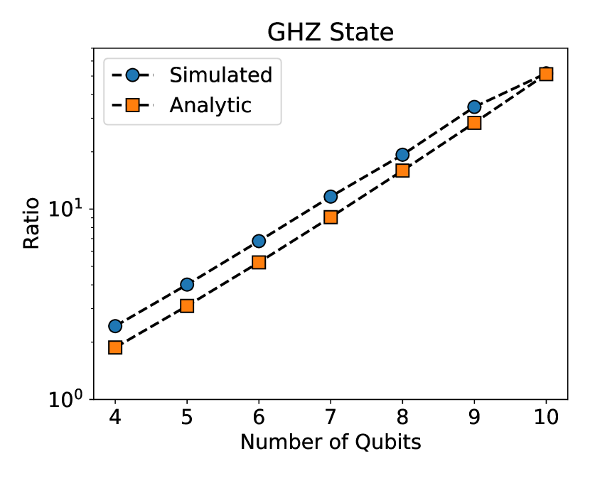
Figure 2: Scaling ratio for the qudit-based quantum memory to perform as well as the qubit-based quantum memory versus the number of qubits for the GHZ state. The ratio grows exponentially as the number of qubits grows.

III.2 Predicted Ratio

The GHZ state, a superposition of only two states, is the simplest state in this study. Generally, the coefficients $\alpha_{j}$ can take any (normalized) set of values. To provide an approximate ratio for an arbitrary state, we start with the general expression of the fidelity using the solution to the Schrödinger equation, Eq. (22),

$$\sqrt{F(t)}=\Big{|}\langle\psi(0)|e^{-\sum_{j}\frac{\gamma_{j}}{2}C_{j}^{\dagger}C_{j}}|\psi(0)\rangle\Big{|}.$$ (13)

Equation (13) is valid for any initial condition, $|\psi(0)\rangle$ and any system with any noise operators, $C_{i}$. To obtain an approximate solution for this equation, we expand the exponential for some target fidelity, $\mathcal{F}_{t}$,

$$\sqrt{\mathcal{F}_{t}}=\sum_{k}\sum_{j}\frac{(-\gamma_{j}t)^{k}}{2^{k}k!}\langle m^{k}_{j}\rangle,$$ (14)

where $\langle m_{j}^{k}\rangle=\big{|}\langle\psi(0)|\big{(}C_{j}^{\dagger}C_{j}\big{)}^{k}|\psi(0)\rangle\big{|}$ are the moments of the operator $C_{j}^{\dagger}C_{j}$ for the state $|\psi(0)\rangle$. This is valid for any state, $|\psi(0)\rangle$, and set of noise operators, $C_{i}$. For example, using a qudit-based quantum memory with only amplitude damping, we have only one noise operator, $b$, whose moments are simply the moments of the number operator for a qudit, $\langle n_{d}^{k}\rangle$. We can rewrite the fidelity expansion of Eq. (14) as

$$\sqrt{\mathcal{F}_{t}}=\sum_{k}\frac{(-\gamma t_{d})^{k}}{2^{k}k!}\langle n_{d}^{k}\rangle.$$ (15)

A similar expansion can be obtained for qubit-based quantum memories,

$$\sqrt{\mathcal{F}_{t}}=\sum_{k}\frac{(-\gamma t_{b})^{k}}{k!}\langle n_{b}^{k}\rangle,$$ (16)

where, analogous to the qudit-based quantum memory, $\langle n_{b}^{k}\rangle=\big{\langle}\psi(0)\big{|}\big{(}\sum_{i}\sigma_{i}^{\dagger}\sigma_{i}\big{)}^{k}\big{|}\psi(0)\big{\rangle}$. The difference in the factor of $2^{k}$ is due to the inclusion of dephasing in the qubit-based quantum memory noise model. Since we have chosen a specific target fidelity, $\mathcal{F}_{t}$, these two equations, Eq. (15) and Eq. (16), can be equated, and an approximation for the ratio of the times to reach the target fidelity can be obtained by truncating the sum to first order:

$$\frac{t_{b}}{t_{d}}\approx\frac{\langle n_{d}\rangle}{2\langle n_{b}\rangle}.$$ (17)

We have shown here that the ratio of the times for the two quantum memories to reach the target fidelity can simply be approximated as the ratio of the average number of excitations in the qudit-based quantum memory compared with double the average number of excitations in the qubit-based quantum memory. To first order, the ratio does not depend on the target fidelity. Higher-order truncations will depend on the target fidelity. For example, keeping terms to second order gives the following equation

$$\frac{t_{b}}{t_{d}}\approx\frac{\langle n_{d}\rangle}{2\langle n_{b}\rangle}+\frac{\gamma}{\langle n_{b}\rangle t_{d}}\Big{(}t_{b}^{2}\langle n_{b}^{2}\rangle-t_{d}^{2}\langle n_{d}^{2}\rangle\Big{)}$$ (18)

which is a transcendental equation, that, in general, is not solvable in closed form. However, specifying a specific target fidelity, $\mathcal{F}_{t}$, and solving truncated forms of eqns. (15) and (16) via, e.g, a root-finding technique is possible. From this second-order expansion, we can see that the our simpler formula, eq. (17), is accurate to first-order in the decay rate, $\gamma$ and has terms that depend on the second moments of the specific quantum state.

The simple first order equation, eq (17), can be intuitively understood as representing the correlation of the quantum state and the noise models that were used to describe the quantum memories. For example, in the qubit-based quantum memory, each excitation (i.e., the qubit in the $|1\rangle$ state) of an individual qubit contributes to the overall noise by being subject to an amplitude damping and dephasing noise channel. However, if the qubit is not excited (i.e., the qubit is in the $|0\rangle$ state), there is no contribution to the overall noise. A superposition of being excited ($|1\rangle$) and not being excited ($|0\rangle$) would contribute only partially to the total amount of noise. Therefore, under this intuitive argument, we can say that the total amount of noise goes as $2\gamma\langle n_{b}\rangle$. Similar arguments can be made for the qudit-based noise model, leading to the total amount of noise being, intuitively, $\gamma\langle n_{d}\rangle$. The ratio of the total amount of noise between the two quantum memories should, then, give some insight into their relative performance. As derived in Eq. (17), this ratio is approximately the ratio of times to reach any target fidelity.

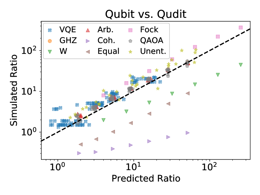
Figure 3: Comparison of the numerically simulated and analytically predicted scaling ratios between a qubit-based quantum memory with both amplitude damping and dephasing and a qudit-based quantum memory with only amplitude damping, for a wide of variety of interesting quantum states. The dashed black line is $y=x$; the closer the points are to this line, the better the prediction.

Figure 3 plots the ratio from data simulated by using the Lindblad master equations for the qubit-based (Eq. (2)) and the qudit-based (Eq. (3)) quantum memories over a wide range of interesting quantum states and sizes. The set of states is discussed in the Theoretical Methods section. System sizes range from $2^{4}$ to $2^{15}$. The line $y=x$ is also indicated on the plot; the closer the points are to this line, the better the prediction of the approximate formula, Eq. (17). The simulated and predicted ratios are highly correlated for most of the states. The coherent and equal superposition states stray far from the line $y=x$. Notably, these two states are the states in which the non-Hermitian dynamics diverges from the full dynamics of the Linblad master equation, as we show in Appendix D. The failure of our predicted ratio is thus because of the failure of the non-Hermitian approximation. For the coherent state, specifically, this is perhaps to be expected, as the full dissipative dynamics have a simple analytically derivable form [43], which is very different than our approximate non-Hermitian form.

This level of agreement is remarkable, given that the derivation of the approximate ratio involves multiple levels of approximation, including both the non-Hermitian approximation used to derive the fidelity equations, eq. (15) and (16), as well as their truncation to first order. The contribution of the truncation was discussed above. To understand the error from the non-Hermitian formalism used to derive the fidelity equations, we compare the full Lindblad dynamics and the non-Hermitian dynamics in Appendix D for the various states studied. Our approximate ratio is surprisingly simple and comprises quantities that can be easily measured in an experimental setting for an arbitrary, unknown quantum state. The use of such a formula is not limited to just the two quantum memories studied here; it is easily generalized to other architectures and can help inform possible strategies for extending the lifetimes of quantum information in quantum memories.

IV Discussion

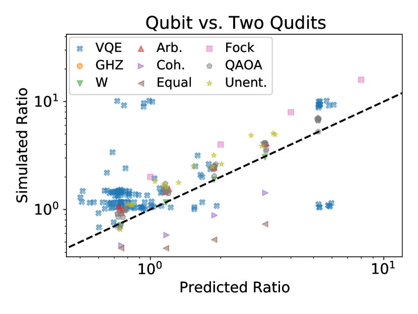
Figure 4: Comparison of the numerically simulated and analytically predicted scaling ratios between a qubit-based quantum memory with both amplitude damping and dephasing and an array of two qudits with only amplitude damping, for many quantum states. The dashed black line is $y=x$; the closer the points are to this line, the better the prediction.

Using either the formal derivation or intuitive arguments, one can easily generate ratios for the performance of other quantum memories. For instance, another potential architecture for a quantum memory is an array of qudits of some intermediate size between a qubit ($d=2$) and a single qudit ($d=2^{n_{q}}$). For illustrative purposes, we choose an array of two qudits with $d=2^{n_{q}-1}$. The predicted ratio is, then,

$$\frac{t_{b}}{t_{\mathrm{int}}}\approx\frac{\langle n_{\mathrm{int}}\rangle}{2\langle n_{b}\rangle},$$ (19)

where the subscript $\mathrm{int}$ denotes the “intermediate” qudit system, $\langle n_{\mathrm{int}}\rangle=\langle\sum_{i}c_{i}^{\dagger}c_{i}\rangle$, and $c_{i}$ is the annihilation operator for the intermediate qudit. Similar comparisons between the intermediate qudit-based quantum memory and single qudit-based quantum memory can also be performed. Figure 4 shows the comparison of the simulated and predicted scaling ratios between a qubit-based quantum memory with both amplitude damping and dephasing and the intermediate qudit-based quantum memory with only amplitude damping. Similar to the comparison to the single qudit-based quantum memory (see Fig. 3), the predicted and simulated ratios are in good agreement. The magnitude of the ratios, both simulated and predicted, are considerably smaller since the average number of excitations in the intermediate qudit-based quantum memory ($\langle n_{\mathrm{int}}\rangle$) is considerably smaller than that in the single qudit-based quantum memory ($\langle n_{d}\rangle$). Approximate performance ratios for other noise models can also be generated within this framework. For example, in many qubit-based quantum devices, the noise rates vary between qubits [67] or even in time [68]. In such a disordered system, our assumption of an equal noise rate, $\gamma$, for all channels breaks down. In this case, instead of using the overall average number of excitations, $\langle n_{b}\rangle$, the average excitation per qubit needs to be weighted by its overall noise contribution, giving

$$\sqrt{\mathcal{F}_{t}}=\sum_{k}\sum_{j}\frac{(-\gamma_{j}t_{dis})^{k}}{k!}\langle n_{j}^{k}\rangle,$$ (20)

where $\langle n_{j}^{k}\rangle=\big{|}\langle\psi(0)|\big{(}\sigma_{j}^{\dagger}\sigma_{j}\big{)}^{k}|\psi(0)\rangle\big{|}$ and we have assumed that the dephasing and amplitude-damping rates are the same for a given qubit but different between qubits. Comparing an ordered qubit register with a disordered qubit register, we find that the approximate ratio of times to reach a target fidelity is, to first order,

$$\frac{t_{b}}{t_{dis}}=\frac{\sum_{j}\gamma_{j}\langle n_{j}\rangle}{\gamma\langle n_{b}\rangle}.$$ (21)

Architectures with other noise channels, beyond amplitude damping and dephasing, can also be included as long as they can be written in the non-Hermitian formalism. There is no guarantee that every noise channel will lead to as simple a formula as Eq. (17), but many will because of the simple relationship of the fidelity to the moments of the operators. A two-qubit correlated amplitude damping channel, for instance, would give a contribution of $\langle n_{b,i}n_{b,j}\rangle$ (in addition to any single-qubit noise).

Our analysis of the correlation of the noise model and the structure of the quantum information can help provide insights into ways to potentially extend the lifetime of quantum states stored in quantum memories. The overall noise, to first order, goes as the number of excitations in the system (regardless of the architecture). Storing the quantum information such that the largest amplitudes are in the lowest possible states will greatly reduce the overall noise and thus increase the effective lifetime of the quantum information. To demonstrate this benefit, we numerically sorted the amplitudes of the quantum states and simulated the performance of a qudit-based quantum memory with only amplitude damping with both the unsorted and sorted quantum states. The comparison between the two layouts is shown in Fig. 5. Reordering states with a small number of amplitudes that happen to be in highly excited states, such as the GHZ and W states, provides a large performance enhancement that grows with system size. Random arbitrary and unentangled states see a modest performance enhancement. The coherent state, on the other hand, actually performs worse after reordering. After reordering, the coherent state is no longer an eigenstate of the annihilation operator and thus loses its superior performance. Reordering the amplitudes of an arbitrary quantum state is generally very expensive; a quantum sort of $n$ items, for example, will take at least $\mathcal{O}\big{(}n\log(n)\big{)}$ steps [69]. However, in the case where classical information is being loaded onto a quantum device through, say, a QRAM technique [70], carefully arranging the amplitudes can increase the performance of the quantum memory, especially in a qudit-based system, where the decay of high Fock states is significantly larger than lower Fock states. Techniques, such as reordering, based on the correlation of the structure of the quantum state with the noise model can be used in addition to quantum error correction [6, 71, 72, 7] and other error mitigation techniques [68, 73, 74].

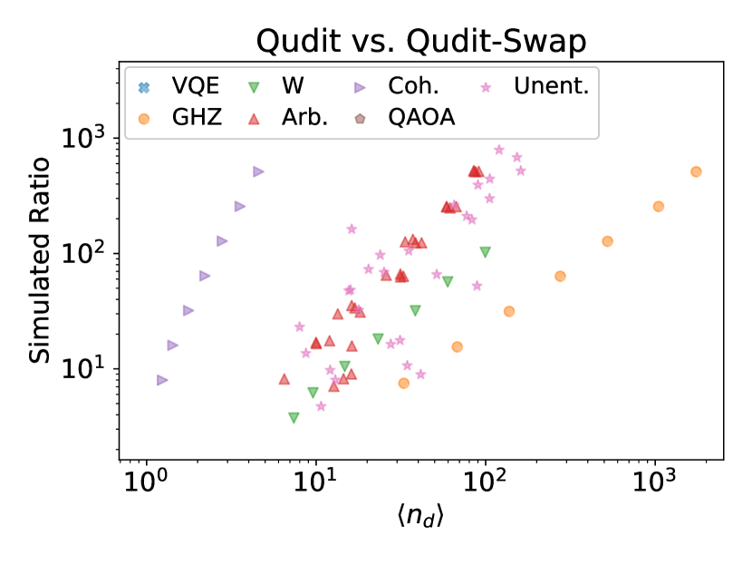
Figure 5: Performance enhancement from reordering the quantum information in a qudit-based quantum memory with amplitude damping. The simulated performance gain grows with increasing average number of excitations in the original state.

	Simulated Ratio	Predicted Ratio
Coherent	0.96	51.29
GHZ	51.67	51.15
W	44.62	51.15
Equal	8.92	51.15
Fock	366.00	256.00
VQE	19.05 $\pm$ 2.04	14.41 $\pm$ 3.88
QAOA	49.44 $\pm$ 3.12	50.72 $\pm$ 0.43
Arbitrary	49.08 $\pm$ 0.14	51.53 $\pm$ 0.38
Unentangled	86.15 $\pm$ 20.89	58.93 $\pm$ 9.32

Table 1: Simulated and predicted performance ratios between a qubit-based quantum memory with both amplitude damping and pure dephasing and a qudit-based quantum memory with only amplitude damping, for a variety of states of size $2^{10}$.

The derived performance ratio, Eq. (17), is an experimentally accessible quantity, even for unknown quantum states, and can be used to understand the relative performance and engineering requirements between quantum architectures. For some given quantum state, choosing between two candidate quantum memory architectures would involve measuring the average number of excitations in either device, as well as knowledge of underlying noise models of each quantum memory. Measuring the average number of excitations is a simple experimental technique that can be done with $\mathcal{O}(1)$ experiments, in both qubits (through standard single-qubit measurements [75]) and qudits (through multilevel quantum tomography techniques [76, 77] or other means), as long as many copies of the quantum state are available. The relative performance between the two quantum memories, assuming equivalent noise rates, could then be predicted by using a formula like Eq. (17). The relative performance could then be compared with the relative noise rates to understand which quantum architecture would perform better. As an explicit example, we return to the qubit-based quantum memory with amplitude damping and pure dephasing and the qudit-based quantum memory with only amplitude damping. For one instance of an arbitrary state of size $2^{4}$ with random wavefunction coefficients, we find that $\langle n_{d}\rangle=8.16$ and $\langle n_{b}\rangle=2.08$, leading to a performance ratio assuming equivalent noise rates, according to Eq. (17), of $\approx 1.96$ (the simulated performance ratio for target fidelity $\mathcal{F}_{t}=0.75$ is 2.44); the qubit-based quantum memory will have reliably stored the quantum state for about twice as long as the qudit-based quantum memory. Put another way, the qudit-based quantum memory would need to have half the noise rate in order to perform as well as the qubit-based quantum memory. Similar comparisons can be made for other quantum states. Table 1 shows the predicted and simulated performance ratios for a variety of quantum states. We find performance ratios on the order of 10–100 for most states of size $2^{10}$, with the coherent state and Fock states being strong outliers. 3D cavity qudits can have $T_{1}$ times that are more than 100$\times$ longer than the $T_{1}$ times of transmon qubits [52, 41] Thus, for states of size $2^{10}\approx 1000$, 3D cavity architectures will likely perform better than qubit-based systems. Above that, a qubit-based system will perform better.

V Concluding Remarks

We presented a detailed study of the interplay between the structure of quantum information and the physical noise models of various quantum memories. We demonstrated simple and experimentally relevant ways of comparing the expected performance of quantum memory architectures for specific quantum states. Although we focused primarily on two paradigmatic devices, superconducting qubits with both amplitude damping and dephasing channels and superconducting cavities with only amplitude damping, our methods can easily be extended to other quantum systems such as trapped ions and photonic systems. We utilized both numerical simulations using the Lindblad master equation and an approximate non-Hermitian formalism to analyze the behavior of a wide variety of interesting and useful quantum states. Our approximate non-Hermitian analysis provides a simple formula that gives intuition on the performance of a given quantum state stored in different devices. As a practical example of the application of our method, we demonstrated that the superconducting cavities are viable candidates for quantum memories up to around 1,000 levels for many classes of states because of their significantly longer $T_{1}$ times. Beyond that, the increased decay from the higher levels lowers the overall fidelity for many of the states, and an array of superconducting qubits becomes a more viable quantum memory. Furthermore, we showed that reducing the total number of excitations in the mapping of data to a quantum state can help increase the overall lifetime of the state and thus provides a way, through state engineering, to increase the performance of a quantum memory device. Our method, given its simplicity and experimental relevance, could be used as part of a heuristic for a quantum compiler for hybrid quantum devices. As long as multiple copies of a state can be created, a simple interrogation of the state, measuring the number of excitations when stored in the various possible subcomponents of the overall device, can be used to decide where to store a state. As the complexity of hybrid quantum devices grows, simple heuristic methods for understanding the performance of each subcomponent, such as the method we present here, will be important for maximizing the overall performance of the device and can help in the initial design.

Appendix A Derivation of Approximate Solution

To derive the approximate solutions of Eq. (8) and Eq. (7), we begin with the generic solution to the non-Hermitian Schrödinger equation of Eq. (6) with initial condition $|\psi(0)\rangle$,

$$|\psi(t)\rangle=e^{-\sum_{j}\frac{\gamma_{j}}{2}C_{j}^{\dagger}C_{j}}|\psi(0)\rangle.$$ (22)

We seek to understand the evolution of the fidelity with respect to the initial state,

$$F(t)=|\langle\psi(0)|\psi(t)\rangle|^{2}.$$ (23)

We derive the following using the square root of the fidelity, $\sqrt{F(t)}$, because of the increased ease of typesetting. We can expand the fidelity using the solution to Schrödinger equation, Eq. 22,

$$\sqrt{F(t)}=|\langle\psi(0)|e^{-\sum_{j}\frac{\gamma_{j}}{2}C_{j}^{\dagger}C_{j}}|\psi(0)\rangle|.$$ (24)

The equation is valid for any initial condition, $|\psi(0)\rangle$ and any system with any noise operators, $C_{i}$. We will now derive specific formulas for several different noise models.

A.1 Single Qudit with Amplitude Damping

A single qudit with amplitude damping has only a single noise operator, the annihiliation operator for an $n$-level system, $b$. We will also expand the initial state in terms of the basis states of the qudit, leading to

$$\sqrt{F(t)}=\sum_{k,j}|\langle j|\alpha_{j}^{*}\alpha_{k}e^{-\frac{\gamma}{2}b^{\dagger}bt}|k\rangle|.$$ (25)

To simplify this expression, we expand the exponential

$$e^{-\frac{\gamma}{2}b^{\dagger}bt}|k\rangle=\sum_{l}\frac{(-\frac{\gamma t}{2})^{l}(b^{\dagger}b)^{l}}{l!}|k\rangle.$$ (26)

Because $b^{\dagger}b|k\rangle=k|k\rangle$, we can rewrite this equation as

$$e^{-\frac{\gamma}{2}b^{\dagger}bt}|k\rangle=\sum_{l}\frac{(-\frac{\gamma t}{2})^{l}(k)^{l}}{l!}|k\rangle=e^{-\frac{\gamma}{2}kt}|k\rangle,$$ (27)

which removes the operator from the exponential. We can now use this simplification in the fidelity expression, Eq. (25). Combining this with the orthonormality of the basis states, we have

$$\sqrt{F(t)}=\sum_{j}|\alpha_{j}|^{2}e^{-\frac{\gamma}{2}jt},$$ (28)

which is the equation in the main text, Eq. (8).

A.2 Qubits with Amplitude Damping and Dephasing

The derivation for other noise models, such as a qubit register with both amplitude damping and dephasing, follows the same logic. The primary difference is the noise operators, $C_{i}$, and how they act on the basis states, $|j\rangle$. For example, on a qubit register, the amplitude damping noise channels are a sum of operators, $\sum_{i}\sigma_{i}^{\dagger}\sigma_{i}$, where $\sigma$ is the annihilation operator for a two-level system. The expansion of the exponential in Eq. (26) changes. The basis states, $|j\rangle$, are now bit strings of length the number of qubits, $n_{q}$. If qubit $i$ is in its excited state, $|1\rangle$, the action of its noise operator $\sigma_{i}^{\dagger}\sigma_{i}$ will return 1; otherwise, it will return 0. The sum of the action of all the amplitude damping noise channels is then just a count of the number of excited qudits in the basis state. This number is known as the Hamming weight, $w(j)$. The dephasing operator, by similar arguments, contributes a term proportional to the Hamming weight. Together, this gives the equation in the main text, Eq. (7).

Appendix B Changing $\mathcal{F}_{t}$

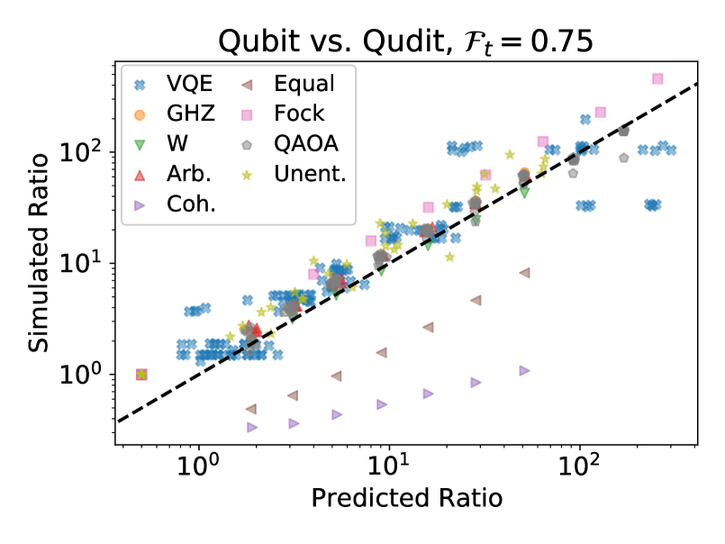
(a) $\mathcal{F}_{t}=0.7$

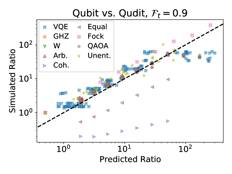
(b) $\mathcal{F}_{t}=0.9$

Figure 6: Comparison of the simulated and predicted scaling ratios between a qubit-based quantum memory with both amplitude damping and dephasing and a qudit-based quantum memory with only amplitude damping, for a wide of variety of interesting quantum states. The two different target fidelities here (in addition to Fig. 3) show that the specific target fidelity does not affect the overall conclusions.

Figure 6 shows the results of applying the analysis of the main text (that is, using the predicted scaling ratio of Eq. (17)) to the various quantum states studied at two target fidelities ($\mathcal{F}_{t}=0.75$ and 0.9). These results, in addition to the results of Fig. 3, all support the efficacy of the scaling prediction. While the predicted ratio is insensitive to the target fidelity, the simulated ratio is sensitive to it. Figure 7 shows the difference between simulated ratios for the GHZ state. The exact position of the simulated ratio changes for GHZ states with larger numbers of excitations in the qudit, but the differences are negligible on the studied scale.

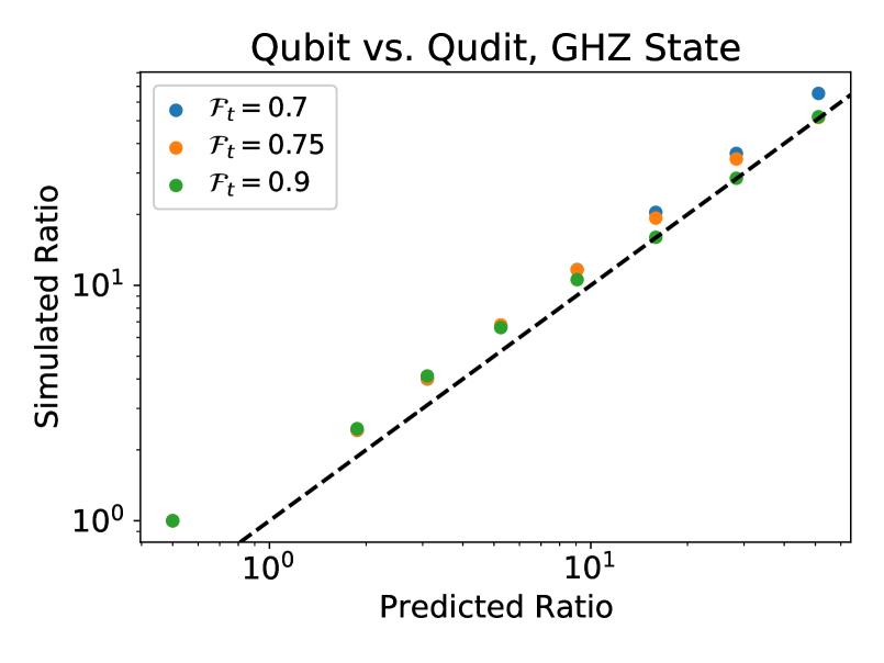
Figure 7: Comparison of the simulated and predicted scaling ratios between a qubit-based quantum memory with both amplitude damping and dephasing and a qudit-based quantum memory with only amplitude damping for the GHZ state at three different target fidelities. While the exact location of the simulated scaling changes, the values are reasonably close.

Appendix C Description of Quantum States

In this section, we describe all the states used in the main text. Unless mentioned otherwise, these states were generated by using utilities available within the QuTiP [78] package.

GHZ State The GHZ state is defined in Eq. (9).

W State The W state for $n_{q}$ qubits is defined as the equal superposition of all states, where one qubit is excited ($|1\rangle$) and all other qubits are in their ground state ($|0\rangle$).

Equal Superposition State The equal superposition state is defined as the state with an equal superposition of all possible basis states.

Fock States A Fock state, or number state, is defined as a state with a specific number of excitations. In this work, we use the Fock states $|8\rangle,$ $|16\rangle,$ $|32\rangle,$ $|64\rangle,$ $|128\rangle,$ $|256\rangle,$ and $|512\rangle$, when represented as a qudit state.

Coherent States A coherent state is generally defined as

$$|\alpha\rangle=e^{-|\alpha|^{2}/2}\sum_{n=0}^{\infty}\frac{\alpha^{n}}{\sqrt{n!}}|n\rangle,$$ (29)

where $\alpha$ is generally a complex number. In this work, however, we focus on quantum systems that have a limit on the number of excitations that can be in the system. We instead use the follow definition,

$$|\alpha\rangle=e^{\alpha(a^{\dagger}-a)}|0\rangle,$$ (30)

where $a$ is a truncated annihilation operator. This definition of the coherent state gives slightly different amplitudes from those obtained with the analytic formula of Eq. (29), especially in the small truncation limit. We use $\alpha=\sqrt{n_{t}/2}$, where $n_{t}$ is the maximum number of excitations allowed in the qudit register and $n_{t}=$ 16, 32, 64, 128, 256, 512, and 1024.

Chemical States To generate states relevant to quantum chemistry studies, we use Qiskit’s Aqua [79] package using parity mapping to map spin orbitals to qubits [80] for all molecules. Rather than solve a variational quantum eigensolver instance, we instead use exact diagonalization to find the exact ground and first excited states for all molecules. We generate states for H₂ with and without two-qubit reduction [80], LiH with two-qubit reduction with and without a frozen core [10], H₄ with and without two-qubit reduction, and H₂O with two-qubit reduction. These states span Hilbert space sizes from 4 to 4,096.

QAOA States To generate quantum approximate optimization algorithm (QAOA) states, we generate Erdős-Rényi graphs [81] of size $n$ with probability $0.5$ of creating an edge between any two nodes. We then use the QAOA solver within Qiskit [79] with $p=4$ steps to solve for the MaxCut of the graph [64]. We generate and solve ten graphs each of size $n=$ 4, 5, 6, 7, 8, 9, 10, 11, and 12.

Arbitrary States We randomly generate arbitrary states by creating dense vectors of uniform random numbers in the range $[-0.5,0.5]$ for both the real and imaginary parts and then normalize the vectors. We create four random states for each total Hilbert space size of 16, 32, 64, 128, 256, 512, and 1024.

Unentangled States We randomly generate unentangled- states as described above for two-level systems and then take the tensor products of several such qubit states to create random, unentangled states. We generate four random states for tensor products of size 4, 5, 6, 7, 8, 9, and 10 qubits.

Appendix D Comparison of Numerical and Analytic Dynamics

We compare the full Lindblad dynamics of both the qubit-based (Eq. (2)) and qudit-based (Eq. (3)) quantum memories with their respective non-Hermitian dynamics in Fig. 8. We find that the non-Hermitian (NH) dynamics, at least for the short-times we are interested in, provides a good approximation for many of the states. For some states, such as the coherent and equal superposition states, the difference in approximation error between the qubit and qudit models is stark. For example, in the coherent state, the qubit system sees good agreement between the full Lindblad dynamics and the approximate non-Hermitian dynamics, but the non-Hermitian dynamics greatly underestimates the true Lindblad dynamics for the qudit system. Correspondingly, this leads to the large errors seen for some of the states in the predicted ratios (see Table 1).

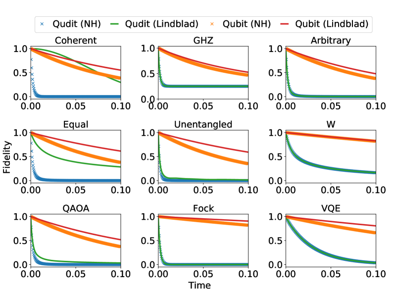
Figure 8: Comparison of the full Lindblad dynamics and the non-Hermitian (NH) approximation for specific $n_{q}=10$ instances of the various states studied.

References

- Lvovsky et al. [2009] A. I. Lvovsky, B. C. Sanders, and W. Tittel, Optical quantum memory, Nature Photonics 3, 706 (2009).
- Dennis et al. [2002] E. Dennis, A. Kitaev, A. Landahl, and J. Preskill, Topological quantum memory, Journal of Mathematical Physics 43, 4452 (2002).
- Ladd et al. [2010] T. D. Ladd, F. Jelezko, R. Laflamme, Y. Nakamura, C. Monroe, and J. L. O’Brien, Quantum computers, Nature 464, 45 (2010).
- Duan et al. [2001] L.-M. Duan, M. D. Lukin, J. I. Cirac, and P. Zoller, Long-distance quantum communication with atomic ensembles and linear optics, Nature 414, 413 (2001).
- Briegel et al. [1998] H.-J. Briegel, W. Dür, J. I. Cirac, and P. Zoller, Quantum repeaters: the role of imperfect local operations in quantum communication, Physical Review Letters 81, 5932 (1998).
- Gottesman [1997] D. Gottesman, Stabilizer codes and quantum error correction, arXiv preprint quant-ph / 9705052 (1997).
- Fowler et al. [2012] A. G. Fowler, M. Mariantoni, J. M. Martinis, and A. N. Cleland, Surface codes: Towards practical large-scale quantum computation, Physical Review A 86, 032324 (2012).
- Preskill [2018] J. Preskill, Quantum computing in the nisq era and beyond, Quantum 2, 79 (2018).
- Arute et al. [2019] F. Arute, K. Arya, R. Babbush, D. Bacon, J. C. Bardin, R. Barends, R. Biswas, S. Boixo, F. G. Brandao, D. A. Buell, et al., Quantum supremacy using a programmable superconducting processor, Nature 574, 505 (2019).
- Kandala et al. [2017] A. Kandala, A. Mezzacapo, K. Temme, M. Takita, M. Brink, J. M. Chow, and J. M. Gambetta, Hardware-efficient variational quantum eigensolver for small molecules and quantum magnets, Nature 549, 242 (2017).
- O‘Malley et al. [2016] P. O‘Malley, R. Babbush, I. Kivlichan, J. Romero, J. McClean, R. Barends, J. Kelly, P. Roushan, A. Tranter, N. Ding, et al., Scalable quantum simulation of molecular energies, Physical Review X 6, 031007 (2016).
- Peruzzo et al. [2014] A. Peruzzo, J. McClean, P. Shadbolt, M.-H. Yung, X.-Q. Zhou, P. J. Love, A. Aspuru-Guzik, and J. L. O’brien, A variational eigenvalue solver on a photonic quantum processor, Nature communications 5, 4213 (2014).
- Edwards et al. [2010] E. Edwards, S. Korenblit, K. Kim, R. Islam, M.-S. Chang, J. Freericks, G.-D. Lin, L.-M. Duan, and C. Monroe, Quantum simulation and phase diagram of the transverse-field ising model with three atomic spins, Physical Review B 82, 060412 (2010).
- Kim et al. [2011] K. Kim, S. Korenblit, R. Islam, E. Edwards, M. Chang, C. Noh, H. Carmichael, G. Lin, L. Duan, C. J. Wang, et al., Quantum simulation of the transverse ising model with trapped ions, New Journal of Physics 13, 105003 (2011).
- Zhang et al. [2017] J. Zhang, G. Pagano, P. W. Hess, A. Kyprianidis, P. Becker, H. Kaplan, A. V. Gorshkov, Z. X. Gong, and C. Monroe, Observation of a many-body dynamical phase transition with a 53-qubit quantum simulator, Nature 551, 601 (2017), arXiv:1708.01044 .
- Kyriienko and Sørensen [2018] O. Kyriienko and A. S. Sørensen, Floquet quantum simulation with superconducting qubits, Physical Review Applied 9, 064029 (2018).
- Schauss [2018] P. Schauss, Quantum simulation of transverse ising models with rydberg atoms, Quantum Science and Technology 3, 023001 (2018).
- Arute et al. [2020] F. Arute, K. Arya, R. Babbush, D. Bacon, J. C. Bardin, R. Barends, A. Bengtsson, S. Boixo, M. Broughton, B. B. Buckley, et al., Observation of separated dynamics of charge and spin in the fermi-hubbard model, arXiv preprint arXiv:2010.07965 (2020).
- Otten et al. [2019] M. Otten, C. L. Cortes, and S. K. Gray, Noise-resilient quantum dynamics using symmetry-preserving ansatzes, arXiv:1910.06284 (2019).
- Chiesa et al. [2019] A. Chiesa, F. Tacchino, M. Grossi, P. Santini, I. Tavernelli, D. Gerace, and S. Carretta, Quantum hardware simulating four-dimensional inelastic neutron scattering, Nature Physics 15, 455 (2019).
- Venturelli et al. [2015] D. Venturelli, S. Mandra, S. Knysh, B. O’Gorman, R. Biswas, and V. Smelyanskiy, Quantum optimization of fully connected spin glasses, Physical Review X 5, 031040 (2015).
- Bengtsson et al. [2020] A. Bengtsson, P. Vikstål, C. Warren, M. Svensson, X. Gu, A. F. Kockum, P. Krantz, C. Križan, D. Shiri, I.-M. Svensson, et al., Improved success probability with greater circuit depth for the quantum approximate optimization algorithm, Physical Review Applied 14, 034010 (2020).
- Otten et al. [2020] M. Otten, I. R. Goumiri, B. W. Priest, G. F. Chapline, and M. D. Schneider, Quantum machine learning using gaussian processes with performant quantum kernels, arXiv preprint arXiv:2004.11280 (2020).
- Havliček et al. [2019] V. Havliček, A. D. Córcoles, K. Temme, A. W. Harrow, A. Kandala, J. M. Chow, and J. M. Gambetta, Supervised learning with quantum-enhanced feature spaces, Nature 567, 209 (2019).
- Awschalom et al. [2020] D. Awschalom, K. K. Berggren, H. Bernien, S. Bhave, L. D. Carr, P. Davids, S. E. Economou, D. Englund, A. Faraon, M. Fejer, S. Guha, M. V. Gustafsson, E. Hu, L. Jiang, J. Kim, B. Korzh, P. Kumar, P. G. Kwiat, M. Lončar, M. D. Lukin, D. A. B. Miller, C. Monroe, S. W. Nam, P. Narang, J. S. Orcutt, M. G. Raymer, A. H. Safavi-Naeini, M. Spiropulu, K. Srinivasan, S. Sun, J. Vučković, E. Waks, R. Walsworth, A. M. Weiner, and Z. Zhang, Development of quantum interconnects for next-generation information technologies, arXiv preprint arXiv:1912.06642 (2020).
- Valivarthi et al. [2020] R. Valivarthi, S. Davis, C. Pena, S. Xie, N. Lauk, L. Narvaez, J. P. Allmaras, A. D. Beyer, Y. Gim, M. Hussein, et al., Teleportation systems towards a quantum internet, arXiv preprint arXiv:2007.11157 (2020).
- Yin et al. [2020] J. Yin, Y.-H. Li, S.-K. Liao, M. Yang, Y. Cao, L. Zhang, J.-G. Ren, W.-Q. Cai, W.-Y. Liu, S.-L. Li, et al., Entanglement-based secure quantum cryptography over 1,120 kilometres, Nature , 1 (2020).
- Gündoğan et al. [2020] M. Gündoğan, J. S. Sidhu, V. Henderson, L. Mazzarella, J. Wolters, D. K. Oi, and M. Krutzik, Space-borne quantum memories for global quantum communication, arXiv preprint arXiv:2006.10636 (2020).
- Krutyanskiy et al. [2019] V. Krutyanskiy, M. Meraner, J. Schupp, V. Krcmarsky, H. Hainzer, and B. P. Lanyon, Light-matter entanglement over 50 km of optical fibre, npj Quantum Information 5, 1 (2019).
- Yu et al. [2020] Y. Yu, F. Ma, X.-Y. Luo, B. Jing, P.-F. Sun, R.-Z. Fang, C.-W. Yang, H. Liu, M.-Y. Zheng, X.-P. Xie, et al., Entanglement of two quantum memories via fibres over dozens of kilometres, Nature 578, 240 (2020).
- Hasegawa et al. [2019] Y. Hasegawa, R. Ikuta, N. Matsuda, K. Tamaki, H.-K. Lo, T. Yamamoto, K. Azuma, and N. Imoto, Experimental time-reversed adaptive bell measurement towards all-photonic quantum repeaters, Nature communications 10, 1 (2019).
- Wang et al. [2020] J. Wang, F. Sciarrino, A. Laing, and M. G. Thompson, Integrated photonic quantum technologies, Nature Photonics 14, 273 (2020).
- Ofek et al. [2016] N. Ofek, A. Petrenko, R. Heeres, P. Reinhold, Z. Leghtas, B. Vlastakis, Y. Liu, L. Frunzio, S. Girvin, L. Jiang, et al., Extending the lifetime of a quantum bit with error correction in superconducting circuits, Nature 536, 441 (2016).
- Neeley et al. [2008] M. Neeley, M. Ansmann, R. C. Bialczak, M. Hofheinz, N. Katz, E. Lucero, A. O’connell, H. Wang, A. N. Cleland, and J. M. Martinis, Process tomography of quantum memory in a josephson-phase qubit coupled to a two-level state, Nature Physics 4, 523 (2008).
- Lai et al. [2018] Y.-Y. Lai, G.-D. Lin, J. Twamley, and H.-S. Goan, Single-nitrogen-vacancy-center quantum memory for a superconducting flux qubit mediated by a ferromagnet, Physical Review A 97, 052303 (2018).
- Monz et al. [2009] T. Monz, K. Kim, A. S. Villar, P. Schindler, M. Chwalla, M. Riebe, C. F. Roos, H. Häffner, W. Hänsel, M. Hennrich, and R. Blatt, Realization of Universal Ion-Trap Quantum Computation with Decoherence-Free Qubits, Physical Review Letters 103, 200503 (2009).
- Sigillito et al. [2019] A. J. Sigillito, M. J. Gullans, L. F. Edge, M. Borselli, and J. R. Petta, Coherent transfer of quantum information in silicon using resonant SWAP gates, npj Quantum Information 5, 10.1038/s41534-019-0225-0 (2019), arXiv:1906.04512 .
- Reagor et al. [2013] M. Reagor, H. Paik, G. Catelani, L. Sun, C. Axline, E. Holland, I. M. Pop, N. A. Masluk, T. Brecht, L. Frunzio, M. H. Devoret, L. Glazman, and R. J. Schoelkopf, Reaching 10 ms single photon lifetimes for superconducting aluminum cavities, Applied Physics Letters 102, 192604 (2013).
- Reshitnyk et al. [2016] Y. Reshitnyk, M. Jerger, and A. Fedorov, 3D microwave cavity with magnetic flux control and enhanced quality factor, EPJ Quantum Technology 3, 13 (2016).
- Xie et al. [2018] E. Xie, F. Deppe, M. Renger, D. Repp, P. Eder, M. Fischer, J. Goetz, S. Pogorzalek, K. G. Fedorov, A. Marx, et al., Compact 3d quantum memory, Applied Physics Letters 112, 202601 (2018).
- Romanenko et al. [2020] A. Romanenko, R. Pilipenko, S. Zorzetti, D. Frolov, M. Awida, S. Belomestnykh, S. Posen, and A. Grassellino, Three-dimensional superconducting resonators at mk with photon lifetimes up to s, Phys. Rev. Applied 13, 034032 (2020).
- Carmichael [2009] H. Carmichael, An open systems approach to quantum optics: lectures presented at the Université Libre de Bruxelles, October 28 to November 4, 1991, Vol. 18 (Springer Science & Business Media, 2009).
- Haroche and Raimond [2006] S. Haroche and J.-M. Raimond, Exploring the quantum: atoms, cavities, and photons (Oxford university press, 2006).
- Gambetta et al. [2008] J. Gambetta, A. Blais, M. Boissonneault, A. A. Houck, D. Schuster, and S. M. Girvin, Quantum trajectory approach to circuit qed: Quantum jumps and the zeno effect, Physical Review A 77, 012112 (2008).
- Otten et al. [2016] M. Otten, J. Larson, M. Min, S. M. Wild, M. Pelton, and S. K. Gray, Origins and optimization of entanglement in plasmonically coupled quantum dots, Physical Review A 94, 022312 (2016).
- Otten et al. [2015] M. Otten, R. A. Shah, N. F. Scherer, M. Min, M. Pelton, and S. K. Gray, Entanglement of two, three, or four plasmonically coupled quantum dots, Physical Review B 92, 125432 (2015).
- MacQuarrie et al. [2017] E. R. MacQuarrie, M. Otten, S. K. Gray, and G. D. Fuchs, Cooling a mechanical resonator with nitrogen-vacancy centres using a room temperature excited state spin–strain interaction, Nature Communications 8, 14358 (2017).
- Remizov et al. [2019] S. V. Remizov, A. A. Zhukov, W. V. Pogosov, and Y. E. Lozovik, Radiation trapping effect versus superradiance in quantum simulation of light-matter interaction, Laser Physics Letters 16, 065205 (2019), arXiv:1909.11900 .
- Paz-Silva et al. [2019] G. A. Paz-Silva, L. M. Norris, F. Beaudoin, and L. Viola, Extending comb-based spectral estimation to multiaxis quantum noise, Physical Review A 100, 042334 (2019).
- Sung et al. [2020] Y. Sung, A. Vepsäläinen, J. Braumüller, F. Yan, J. I.-J. Wang, M. Kjaergaard, R. Winik, P. Krantz, A. Bengtsson, A. J. Melville, B. M. Niedzielski, M. E. Schwartz, D. K. Kim, J. L. Yoder, T. P. Orlando, S. Gustavsson, and W. D. Oliver, Multi-level Quantum Noise Spectroscopy, arXiv preprint arXiv:2003.02782 (2020).
- Krantz et al. [2019] P. Krantz, M. Kjaergaard, F. Yan, T. P. Orlando, S. Gustavsson, and W. D. Oliver, A quantum engineer’s guide to superconducting qubits, Applied Physics Reviews 6, 021318 (2019).
- Reagor et al. [2016] M. Reagor, W. Pfaff, C. Axline, R. W. Heeres, N. Ofek, K. Sliwa, E. Holland, C. Wang, J. Blumoff, K. Chou, M. J. Hatridge, L. Frunzio, M. H. Devoret, L. Jiang, and R. J. Schoelkopf, Quantum memory with millisecond coherence in circuit qed, Phys. Rev. B 94, 014506 (2016).
- Harty et al. [2014] T. Harty, D. Allcock, C. J. Ballance, L. Guidoni, H. Janacek, N. Linke, D. Stacey, and D. Lucas, High-fidelity preparation, gates, memory, and readout of a trapped-ion quantum bit, Physical review letters 113, 220501 (2014).
- Acín et al. [2001] A. Acín, D. Bruß, M. Lewenstein, and A. Sanpera, Classification of Mixed Three-Qubit States, Physical Review Letters 87, 040401 (2001).
- Otten [2017] M. Otten, QuaC: Open quantum systems in C, a time-dependent open quantum systems solver, https://github.com/0tt3r/QuaC (2017).
- Arfken and Weber [1999] G. B. Arfken and H. J. Weber, Mathematical methods for physicists (1999).
- Dür et al. [2000] W. Dür, G. Vidal, and J. I. Cirac, Three qubits can be entangled in two inequivalent ways, Physical Review A 62, 062314 (2000).
- Degen et al. [2017] C. Degen, F. Reinhard, and P. Cappellaro, Quantum sensing, Reviews of Modern Physics 89, 035002 (2017).
- Yu et al. [2017] Q. Yu, Y. Zhang, J. Li, H. Wang, X. Peng, and J. Du, Generic preparation and entanglement detection of equal superposition states, Science China Physics, Mechanics & Astronomy 60, 070313 (2017).
- Deutsch and Jozsa [1992] D. Deutsch and R. Jozsa, Rapid solution of problems by quantum computation, Proceedings of the Royal Society of London. Series A: Mathematical and Physical Sciences 439, 553 (1992).
- Macridin et al. [2018] A. Macridin, P. Spentzouris, J. Amundson, and R. Harnik, Digital quantum computation of fermion-boson interacting systems, Physical Review A 98, 042312 (2018).
- Colless et al. [2018] J. Colless, V. Ramasesh, D. Dahlen, M. Blok, M. Kimchi-Schwartz, J. McClean, J. Carter, W. de Jong, and I. Siddiqi, Computation of Molecular Spectra on a Quantum Processor with an Error-Resilient Algorithm, Physical Review X 8, 011021 (2018).
- Farhi et al. [2014] E. Farhi, J. Goldstone, and S. Gutmann, A quantum approximate optimization algorithm, arXiv preprint arXiv:1411.4028 (2014).
- Shaydulin et al. [2019] R. Shaydulin, H. Ushijima-Mwesigwa, I. Safro, S. Mniszewski, and Y. Alexeev, Network community detection on small quantum computers, Advanced Quantum Technologies 2, 1900029 (2019).
- Cortes et al. [2020] C. L. Cortes, M. Otten, and S. K. Gray, Non-hermitian approach for quantum plasmonics, The Journal of Chemical Physics 152, 084105 (2020).
- Mølmer et al. [1993] K. Mølmer, Y. Castin, and J. Dalibard, Monte carlo wave-function method in quantum optics, JOSA B 10, 524 (1993).
- Tannu and Qureshi [2018] S. S. Tannu and M. K. Qureshi, A case for variability-aware policies for nisq-era quantum computers, arXiv preprint arXiv:1805.10224 (2018).
- Kandala et al. [2019] A. Kandala, K. Temme, A. D. Córcoles, A. Mezzacapo, J. M. Chow, and J. M. Gambetta, Error mitigation extends the computational reach of a noisy quantum processor, Nature 567, 491 (2019).
- Høyer et al. [2001] P. Høyer, J. Neerbek, and Y. Shi, Quantum complexities of ordered searching, sorting, and element distinctness, in International Colloquium on Automata, Languages, and Programming (Springer, 2001) pp. 346–357.
- Giovannetti et al. [2008] V. Giovannetti, S. Lloyd, and L. MacCone, Quantum random access memory, Physical Review Letters 100, 160501 (2008), arXiv:0708.1879 .
- Leghtas et al. [2013] Z. Leghtas, G. Kirchmair, B. Vlastakis, R. J. Schoelkopf, M. H. Devoret, and M. Mirrahimi, Hardware-efficient autonomous quantum memory protection, Physical Review Letters 111, 120501 (2013).
- Raussendorf and Harrington [2007] R. Raussendorf and J. Harrington, Fault-tolerant quantum computation with high threshold in two dimensions, Physical review letters 98, 190504 (2007).
- Otten and Gray [2019a] M. Otten and S. K. Gray, Accounting for errors in quantum algorithms via individual error reduction, npj Quantum Information 5, 11 (2019a).
- Otten and Gray [2019b] M. Otten and S. K. Gray, Recovering noise-free quantum observables, Physical Review A 99, 012338 (2019b).
- Naghiloo [2019] M. Naghiloo, Introduction to experimental quantum measurement with superconducting qubits, arXiv preprint arXiv:1904.09291 (2019).
- Chakram et al. [2020a] S. Chakram, A. E. Oriani, R. K. Naik, A. V. Dixit, K. He, A. Agrawal, H. Kwon, and D. I. Schuster, Seamless high-q microwave cavities for multimode circuit qed, arXiv preprint arXiv:2010.16382 (2020a).
- Chakram et al. [2020b] S. Chakram, K. He, A. V. Dixit, A. E. Oriani, R. K. Naik, N. Leung, H. Kwon, W.-L. Ma, L. Jiang, and D. I. Schuster, Multimode photon blockade, arXiv preprint arXiv:2010.15292 (2020b).
- Johansson et al. [2012] J. Johansson, P. Nation, and F. Nori, QuTiP: An open-source Python framework for the dynamics of open quantum systems, Computer Physics Communications 183, 1760 (2012).
- Aleksandrowicz et al. [2019] G. Aleksandrowicz, T. Alexander, P. Barkoutsos, L. Bello, Y. Ben-Haim, D. Bucher, F. Cabrera-Hernández, J. Carballo-Franquis, A. Chen, C. Chen, et al., Qiskit: An open-source framework for quantum computing, Accessed on: Mar 16 (2019).
- Bravyi et al. [2017] S. Bravyi, J. M. Gambetta, A. Mezzacapo, and K. Temme, Tapering off qubits to simulate fermionic hamiltonians, arXiv preprint arXiv:1701.08213 (2017).
- Erdős and Rényi [1960] P. Erdős and A. Rényi, On the evolution of random graphs, Publ. Math. Inst. Hung. Acad. Sci 5, 17 (1960).