Quadruply-imaged quasars: some general features

1 INTRODUCTION

Strong gravitational lensing is an important tool for astrophysics observations, in particular by amplifying the observed brightness of sources of the early Universe and thereby allowing for reaching farther out than would otherwise be possible. Numerous textbooks and journal articles are dedicated to its study. The present article addresses the case of a specific sample of gravitationally lensed quasars, those for which four separated images have been observed. Systematic studies of such systems, called quads in the gravitational lensing jargon, are available in the literature. Many of these study the case of a nearly isotropic lensing potential, the anisotropy being described to first order only. Indeed, in most practical real cases, such a treatment is known to provide a good description of the image configuration. In many cases, the anisotropy is due to a slightly aspherical mass distribution of the lensing galaxy, in which case it is natural to describe it with an ellipticity term; in many other cases it is due to the tidal effect of other galaxies in the neighbourhood of the lens, in which case it is best described by a quadrupole tidal shear term. Both descriptions give similar results but Kovner (1987) was first to underline the outstanding simplicity of the latter description. He remarked that independently from the orientation and scale of the images, their configuration depends on a single parameter, the tidal shear, and that the lens equation reduces to a single equation having this parameter as unknown. He gave recipes to solve it graphically and stated some general rules relating the image multiplicity to the position of the source in the lens caustic. A few years later, together with Kassiola (Kassiola & Kovner, 1995) he used the same simple lensing potential to construct two parameters allowing for an educated guess to be made of whether the lens has a simple mass distribution. Meanwhile, together with Blandford and Kochanek (Blandford et al., 1989) he had produced a first comprehensive review of gravitational lensing, a field of astrophysics that was then developing rapidly. In 2003, in the same spirit of simplicity, Saha & Williams (2003) remarked that some characteristics of multiply imaged QSO systems are very model independent and can be deduced accurately by simply scrutinizing the image configuration; depending on the position of the source relative to the caustic they identified four kinds of quadruple systems which they named core quads, inclined quads, long-axis quads and short-axis quads. An illustration is given in Figure 1. Other names have been later used by other authors, such as crosses, folds and cusps (Keeton et al., 2003, 2005), the latter class including both the long-axis and short-axis quads of the Saha & Williams classification; indeed, the distinction between the two is only possible when the lensing potential is significantly aspherical. A decade later, again in the same spirit of obtaining simply useful information about the lensing mechanism without any recourse to mass modelling, Woldesenbet & Williams (2012) have shown that the three opening angles defining the image configuration are strongly correlated, a result that remains valid when the tidal shear or ellipticity term takes relatively large values. They investigate how well this correlation is obeyed by observed quads and discuss cases where deviations are significant, such as for RX J0911. Another form of the correlation obeyed by quads was found by Witt (1996): the four images, the quasar and the lens are located on a same rectangular hyperbola whose asymptotes align with the potential major and minor axes; last year, Schechter & Wynne (2019) examined how well this correlation is obeyed by observed quads. Our work is in the legacy of these authors, particularly of that of Woldesenbet & Williams (2012), extending their analysis to radial distances as well as opening angles and basing it on the quasar images exclusively without requiring the lens to be observed.

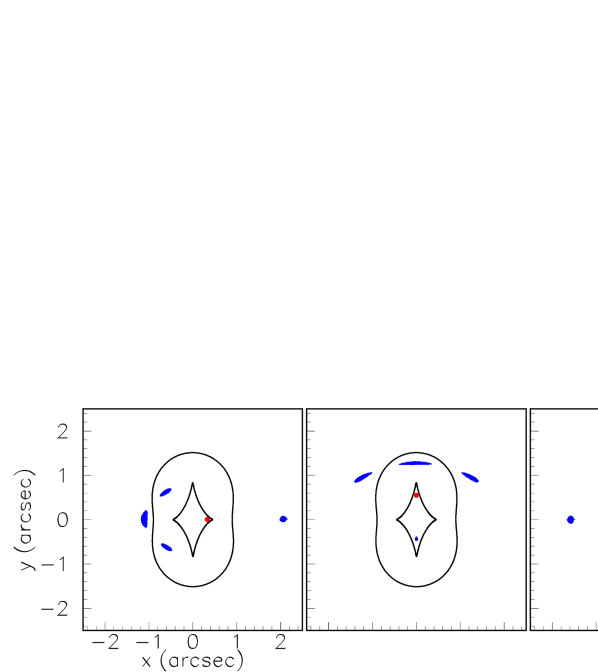
Figure 1: Typical quadruply-imaged quasars according to Saha & Williams (2003) classification. Both images and sources are shown on the plane of the sky ($x,y$). The images (blue areas) are of a disc source (red disc) having a radius of 0.05 arcsec; the caustic and critical curves are shown as black lines (from Hoai et al. 2013). From left to right: short axis quad, long axis quad, core quad and inclined quad.

Some two decades ago, a collaboration between scientists at the Harvard-Smithsonian Center for Astrophysics and the University of Arizona (Falco et al., 1999) took the initiative to carry out a complete survey of all known galaxy-mass gravitational lens systems with image separations of less than 10 arcseconds. The survey, named CASTLeS for CfA-Arizona Space Telescope Lens Survey, used the Hubble Space Telescope (HST) to obtain deep, high-resolution images in the optical and near infrared. Since then, the collaboration continues to maintain a web site (CASTLeS ) updated with the latest HST observations of lens systems. It constitutes a very precious data base that is used by many authors. The present article studies a subset of the CASTLeS data base made of quadruply-imaged quasars with the aim of offering a new illustration of the remarkable properties of gravitational lensing optics.

2 THE DATA SAMPLE

2.1 Normalised coordinates

We select from the list of quadruply-imaged systems (quads) compiled by CASTLeS those for which the identity of the four images and of the lens seem to be reliably assessed. This leaves us with 23 cases listed in Table 1. In a first step we produce, for each quad, parameters that define its configuration independently from its location, orientation and size. As the lens is often more difficult to identify than the images, we ignore it in our definition of normalised coordinates, which does not require the lens to be detected. Precisely, we choose coordinates in the sky plane, $x$=$r\cos\theta$ and $y$=$r\sin\theta$, such that for each quad $\sum_{1,4}x_{i}$=$\sum_{1,4}y_{i}$=0. The resulting values of $r_{i}$=$(x_{i}^{2}+y_{i}^{2})^{1/2}$ provide a measure of the extension of the quad, $R_{0}$=$0.5\{\sum_{1,4}r_{i}^{2}\}^{1/2}$, listed in Table 1. Their list shows an outstanding case, that of SDSS J1004+4112, with $R_{0}$=7.4 arcsec compared with mean$\pm$rms values of 0.9$\pm$0.4 arcsec for the rest of the sample. It is a quasar at redshift $z_{S}\sim$1.7, lensed by a cluster of galaxies at $z_{L}\sim$0.7, that has been described by Oguri et al. (2004). Taking $R_{0}$ as unit of angular separation and choosing the orientation of the axes such that the image having the largest value of $r$ is on the positive part of the $x$ axis, leaves us with eight image coordinates, $(x_{i},y_{i})_{i=1,4}$, obeying four relations:

$$\sum_{1,4}x_{i}=0;\hskip 5.69046pt\sum_{1,4}y_{i}=0;\hskip 5.69046pt\sum_{1,4}r_{i}^{2}=4;\hskip 5.69046pty_{1}=0\hskip 5.69046pt(x_{1}>0)$$

Table 1: The CASTLeS quad sample. Here $r_{ij}$ and $\theta_{ij}$ are defined in Section 2.2 together with $r^{*}_{ij}$ and $\theta^{*}_{ij}$; $x_{L}$ and $y_{L}$ are normalised lens coordinates that are studied in Section 3.4.

Nr	Name	$R_{0}(\textit{mas})$	$r_{13}/r_{13}^{*}(\%)$	$\theta_{24}$ / $\theta^{*}_{24}(\text{${}^{\circ}$})$	$r_{24}/r_{24}^{*}(\%)$	$\theta_{13}/\theta^{*}_{13}(\text{${}^{\circ}$})$	$x_{L}(\%)$	$y_{L}(\%)$	$\delta_{13}/\delta_{24}$
1	PMNJ0134-0931	332	85/78	241/248	12/13	195/194	$-$49	$-$1	1.2/0.2
2	HE0230-2130	988	18/23	200/196	23/20	197/201	$-$11	37	0.7/0.7
3	MG0414+0534	1116	54/53	223/224	$-$35/$-$37	145/146	40	$-$12	0.3/0.3
4	HE0435-1223	1201	2/5	182/179	$-$19/$-$16	170/167	0	$-$14	0.4/0.7
5	B0712+472	642	63/63	233/233	$-$19/$-$27	148/156	58	1	0.0/1.6
6	HS0810+2554	463	53/52	222/223	$-$29/$-$31	150/152	28	$-$7	0.2/0.4
7	RXJ0911+0551	1377	98/110	289/278	6/1	178/183	1	2	2.0/1.0
8	SDSS0924-0219	863	41/39	209/211	$-$21/$-$19	165/163	14	$-$12	0.4/0.3
9	SDSS1004+4112	7412	45/45	217/217	$-$46/$-$41	147/142	3	$-$45	0.0/1.1
10	SDSS1011+0143	1845	7/9	184/183	15/11	188/192	$-$1	2	0.3/0.9
11	PG1115+080	1146	49/50	223/222	20/22	204/203	12	17	0.2/0.3
12	RXJ1131-1231	1565	86/78	240/247	2/0	180/182	66	$-$1	1.3/0.4
13	SDSS1138+0314	668	19/19	193/193	$-$21/$-$18	168/164	4	$-$15	0.1/0.7
14	HST12531-2914	613	7/8	184/183	$-$26/$-$21	167/162	$-$2	$-$17	0.2/1.1
15	HST14113+5211	925	8/11	187/185	8/5	184/187	2	14	0.5/0.5
16	H1413+117	617	2/5	182/180	$-$15/$-$12	172/170	6	$-$12	0.5/0.5
17	HST14176+5226	1430	8/10	186/184	$-$12/$-$10	173/172	$-$4	$-$10	0.4/0.4
18	B1422+231	677	68/58	221/229	$-$14/$-$16	164/166	89	0	1.5/0.5
19	B1555+375	226	53/51	222/223	$-$32/$-$34	147/149	26	$-$5	0.2/0.4
20	WF12026-4536	658	59/58	227/229	12/14	198/195	19	11	0.2/0.5
21	WF12033-4723	1148	49/49	220/220	$-$27/$-$25	160/158	10	$-$22	0.0/0.5
22	B2045+265	872	104/106	275/274	$-$7/$-$10	169/172	98	0	0.3/0.6
23	Q2237+030	877	7/9	185/183	$-$24/$-$20	167/163	0	$-$20	0.3/0.8

2.2 Correlations

The definition of normalised image coordinates described in the preceding paragraph leaves four parameters defining the quad configuration independently from location, orientation and size. We find it convenient to express these in terms of the image polar coordinates, $r_{i}$ and $\theta_{i}$=$\tan^{-1}(y_{i}/x_{i})$. We rank the images in order of increasing values of $\theta_{i}$, which we choose to define between 0 and 360^∘($\theta_{1}$=0).

Figure 2: Normalised coordinates of the CASTLeS quad sample. From left to right: distribution of $r$; correlation between $\theta_{24}$ (abscissa) and $r_{13}$ (ordinate); correlation between $\theta_{13}$ (abscissa) and $r_{24}$ (ordinate). The lines show the relations illustrated in Table 2.

The reason for using polar coordinates is that they are better adapted to describe correlations such as suggested by Saha & Williams (2003). We note in particular the presence of a strong correlation between the opening angle of a pair of images of equal parity (1$-$3 or 2$-$4) and the difference between the $r$ values of the other pair. Figure 2 displays the correlation between $\theta_{13}$=$\theta_{3}$ and $r_{24}$=$r_{2}-r_{4}$ together with the correlation between $\theta_{24}$=360^∘+$\theta_{2}-\theta_{4}$ and $r_{13}$=$r_{1}-r_{3}$. Other combinations of normalised coordinates have been considered and found to display significant correlation, however much weaker. Part of the observed correlation is trivial and simply results from the definition of normalised coordinates. A qualitative illustration is shown in Figure 3, which displays the correlation plots of Figure 2 for a random distribution of images in a region of the sky covering a solid angle of similar size as that covered by the CASTLeS quad sample. While significantly weaker, the correlation is important. A quantitative evaluation of the correlation caused by the lensing mechanism proper is given in Section 3.

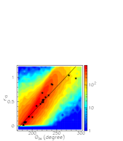
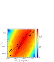
Figure 3: Normalised coordinate distributions of images uniformly distributed in a square covering a solid angle of similar size as that covered by the CASTLeS quad sample. From left to right: distribution of $r$; correlation between $\theta_{24}$ (abscissa) and $r_{13}$ (ordinate); correlation between $\theta_{13}$ (abscissa) and $r_{24}$ (ordinate). The CASTLeS quad sample is overplotted in the two right-most panels.

2.3 Two parameters to define a quad configuration

The strong correlations illustrated in Figure 2 are an invitation to using only two parameters to define the intrinsic configuration of each quad. For example, we might choose $\theta_{13}$ and $\theta_{24}$ and obtain approximate values of $r_{13}$ and $r_{24}$ by assuming that the observed correlations are exactly obeyed. Writing the correlations in the form $r_{ij}=a_{ij}\theta_{kl}+b_{ij}$ the values of the coefficients are listed in Table 2 together with the values of $\Delta r_{ij}=\{\sum_{1,23}(r_{ij}-a_{ij}\theta_{kl}-b_{ij})^{2}/23\}^{1/2}$ which measures how well the correlation is obeyed globally by the sample of 23 quads. We also list the equivalent quantity $\Delta\theta_{kl}=\{\sum_{1,23}(\theta_{kl}-r_{ij}/a_{ij}+b_{ij}/a_{ij})^{2}/23\}^{1/2}$. For each quad, we calculate the values of $\theta_{kl}$ and $r_{ij}$, which we call $\theta^{*}_{kl}$ and $r^{*}_{ij}$ respectively, which obey exactly the correlation and are as close as possible from $\theta_{kl}$ and $r_{ij}$ within $\Delta\theta_{kl}$ and $\Delta r_{ij}$. Precisely,

$$\theta^{*}_{kl}= \theta_{kl}+a_{ij}(r_{ij}-a_{ij}\theta_{kl}-b_{ij})/[a^{2}_{ij}+(\Delta r_{ij}/\Delta\theta_{kl})^{2}]$$

$$r^{*}_{ij}= r_{ij}-(\Delta r_{ij}/\Delta\theta_{kl})^{2}(r_{ij}-a_{ij}\theta_{kl}-b_{ij})/$$

$$[a^{2}_{ij}+(\Delta r_{ij}/\Delta\theta_{kl})^{2}]$$

The values of ($r_{ij},r^{*}_{ij}$) and of ($\theta_{kl},\theta^{*}_{kl}$) are listed in Table 1 together with the values of $\delta_{ij}=\{(r_{ij}-r^{*}_{ij})^{2}$/$\Delta r^{2}_{ij}+(\theta_{kl}-\theta^{*}_{kl})^{2}$/$\Delta\theta^{2}_{kl}\}^{1/2}$, which measure how well the correlation is obeyed by each quad separately.

Table 2: Parameters defining the observed correlations. They are defined as $r_{ij}=a_{ij}\theta_{kl}+b_{ij}$ or equivalently $\theta_{kl}=r_{ij}/a_{ij}-b_{ij}/a_{ij}$. $\Delta r_{ij}$ and $\Delta\theta_{kl}$ are defined in Section 2.3 and measure how well the correlation is obeyed by the CASTLeS quad sample.

$ijkl$	$a$	$b$	$1/a$	$-b/a$	$\Delta r_{ij}$	$\Delta\theta_{kl}(\text{${}^{\circ}$})$
1324	0.0107	$-$1.87	94	175	0.086	8.0
2413	0.0104	$-$1.89	96	182	0.069	6.6

We note that if the CASTLeS sample were large enough, symmetry would impose that $\theta_{ij}$=180^∘ when $r_{kl}$=0, namely $-b_{kl}/a_{kl}$=180^∘.

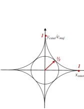
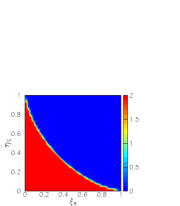
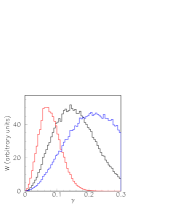
Figure 4: Left: the caustic curve in the $y_{caus}$/$c_{maj}$ vs $x_{caus}$/$c_{min}$ plane. Centre: generated distribution in the $\eta_{S}$ vs $\xi_{S}$ plane. Right: $\gamma$ distributions for $\sigma_{\gamma}=0.05$ (red), 0.10 (black) and 0.15 (blue).

3 A SIMPLE LENS MODEL

3.1 The model

We now compare the prediction of a simple lens model with the results obtained in the preceding section. We assume that the CASTLeS quad sample consists of quad images of quasar point sources, lensed by a simple potential. The justification for such an assumption is that in most cases the parameters of such a potential have effectively been obtained (references are given in the CASTLeS web site). The simplest deviation from an isotropic potential of Einstein radius $R_{E}$ is obtained by breaking isotropy, which implies two parameters defining respectively the amplitude and position angle of the symmetry breaking term. This is usually done by allowing for ellipticity or by introducing an external shear. Here we choose the latter option and write the lensing potential as $\psi=R_{E}r+1/2\gamma r^{2}\cos 2(\theta-\theta_{\gamma})$. It depends on three parameters, the Einstein radius $R_{E}$ and the external shear $\gamma$ at position angle $\theta_{\gamma}$. As $R_{E}$ fixes the scale, we can take it equal to unity since we work in normalised coordinates; and for the same reason the direction to which $\gamma$ is pointing is irrelevant: we set $\theta_{\gamma}$=0 and our lens model effectively depends on a single parameter, the amplitude $\gamma$ of the external shear.

The equation of the caustic is given in parameterised form (parameter $\varphi$):

$$x_{caus}=\{2\gamma/(1+\gamma)\}\cos^{3}\varphi;\quad y_{caus}=\{2\gamma/(1-\gamma)\}\sin^{3}\varphi$$

The semi-minor axis of the caustic ($\varphi$=0^∘) is on the $x$ axis with size $c_{min}=2\gamma/(1+\gamma)$ and its semi-major axis ($\varphi$=90^∘) is on the $y$ axis with size $c_{maj}=2\gamma/(1-\gamma)$. Its equation reads then simply: $x_{caus}=c_{min}\cos^{3}\varphi$; $y_{caus}=c_{maj}\sin^{3}\varphi$ and $\tan\theta=y_{caus}/x_{caus}=(c_{maj}/c_{min})\tan^{3}\varphi$. The equation of the critical curve is $r_{cc}=(1-\gamma\cos 2\theta_{cc})/(1-\gamma^{2})$; its semi-minor and semi-major axes have sizes 1/(1$\pm\gamma$), namely scaled up by a factor (2$\gamma$)^-1 with respect to those of the caustic. For given values of the source location ($x_{S},y_{S}$) inside the caustic and of the external shear $\gamma$ we obtain the quad configuration in terms of the normalised coordinate parameters defined in the preceding section ($r_{13},r_{24},\theta_{13}$ and $\theta_{24}$).

In practice $\gamma$ takes modest values. If it were to require large values it would mean that the lens has a complex structure and the simple form of the potential would probably not be justified. We choose for it a Gaussian distribution of the form exp($-0.5\gamma^{2}$/$\sigma^{2}_{\gamma}$) as illustrated in the right panel of Figure 4. As has been amply remarked by previous authors (Saha & Williams, 2003; Woldesenbet & Williams, 2012) the precise value taken by $\gamma$ has little impact on the image configuration once expressed in a form independent of orientation and scale. In what follows we take as default value $\sigma_{\gamma}=0.1$, covering a broad scale of $\gamma$ values between 0 and 0.3.

The size of the quads is at the scale of unity, as is the size of the critical curve which the four images bracket. Indeed, averaging over $\gamma$, $x_{S}$ and $y_{S}$, we find that $r$ has mean$\pm$rms values of 0.97$\pm$0.23. When $\gamma$ approaches 0, the caustic collapses into a single point at the origin and the critical curve becomes the circular Einstein ring on which the positions of the four images are no longer defined. In practice, for an extended source, the extension of the images becomes such that they cover the whole ring. The probability for a quasar to be located inside the caustic of a lens of external shear $\gamma$ is proportional to the area of the caustic, namely proportional to $\gamma^{2}/(1-\gamma^{2})$. Our sample of model quads (Figure 4) is therefore obtained by generating a uniform source distribution inside a caustic of shear $\gamma$, also uniformly distributed, and giving each quad a weight $W=\gamma^{2}(1-\gamma^{2})^{-1}\text{exp}(-0.5\gamma^{2}/\sigma^{2}_{\gamma})$.

Rather than $x_{S}$ and $y_{S}$, which depend on $\gamma$, we use coordinates that define the position of the source inside the caustic independently from $\gamma$. Precisely, as the quad configuration is independent from the signs of $x_{S}$ and $y_{S}$, we use coordinates $\xi_{S}=|x_{S}|/c_{min}$ and $\eta_{S}=|y_{S}|/c_{maj}$. Both take values between 0 and 1 and are uniformly distributed in the plane (Figure 4).

3.2 Model predictions: general features

Figure 5 compares the quad configurations predicted by the model for $\sigma_{\gamma}$=0.1 with those of the CASTLeS sample. Axial symmetry is observed as expected about $\theta_{13}$=180^∘, $r_{24}$=0 and $y_{L}$=0.

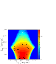
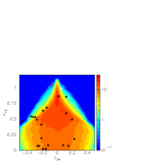
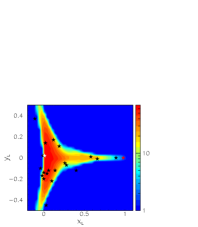
Figure 5: Lens model distributions ($\sigma_{\gamma}$=0.1) in the $\theta_{24}$ vs $\theta_{13}$ plane (left), in the $r_{13}$ vs $r_{24}$ plane (centre) and in the $y_{L}$ vs $x_{L}$ plane (right, see Section 3.4). The stars show the CASTLeS quads (white and red stars are for nr 7 and 22 respectively, see Section 3.3). Units are arbitrary.

Figure 6 shows that the normalised coordinate parameters of the modelled images are strongly correlated in the same way as observed in the CASTLeS quad sample. While expected, this result gives confidence in the validity of the interpretation of the CASTLeS quad sample as quadruply-imaged point sources by a simple lens potential. We have checked that changing $\sigma_{\gamma}$ to 0.05 or 0.15 instead of 0.1 has little influence on this result.

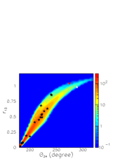
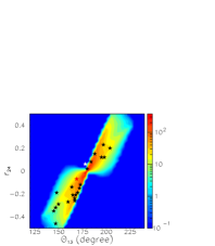
Figure 6: Lens model correlations. From left to right: distribution of $r$; correlation between $\theta_{24}$ (abscissa) and $r_{13}$ (ordinate); correlation between $\theta_{13}$ (abscissa) and $r_{24}$ (ordinate). The stars show the CASTLeS quads (white and red stars are for nr 7 and 22 respectively, see Section 3.3). Units are arbitrary.

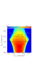
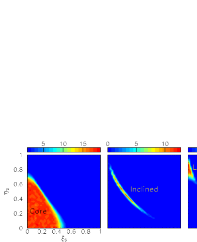
Figure 7: Saha & Williams classification: correlation between the quad configuration in the $\theta_{24}$ vs $\theta_{13}$ plane (left panel) and the location of the source in the $\eta_{S}$ vs $\xi_{S}$ plane. The three right-most panels are, from left to right, for core quads, inclined quads and short or long axis quads respectively, as defined in the left panel: core quads as $\theta_{24}$$<$220^∘, inclined quads as $\theta_{24}$$>$220^∘& $|\theta_{13}-180\text{${}^{\circ}$}|$$>$30^∘, long and short axis quads as $\theta_{24}$$>$220^∘& $|\theta_{13}-180\text{${}^{\circ}$}|$$<$30^∘. The model uses $\sigma_{\gamma}$=0.1.

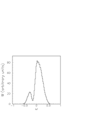
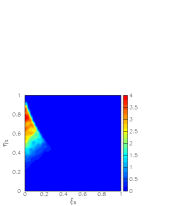
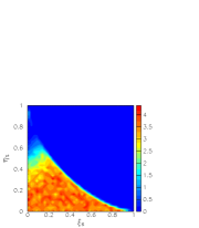
Figure 8: Left: distribution of $\omega$. Centre and right: distributions in the the $\eta_{S}$ vs $\xi_{S}$ plane of quads having $\omega$$<$$-$0.16 (central panel) or $\omega$$>$$-$0.16 (right panel).

The Saha & Williams classification implies a strong correlation between the location of the quasar point source inside the lens caustic and the quad configuration. We describe the latter by the four normalised coordinate parameters, $\theta_{24}$, $\theta_{13}$, $r_{13}$ and $r_{24}$, approximately reducible to only two, $\theta_{24}$ and $\theta_{13}$ or $r_{13}$ and $r_{24}$. Figure 7 illustrates the correlation for quad configurations defined in the $\theta_{24}$ vs $\theta_{13}$ plane. We choose as limits between the core, inclined and cusp classes $\theta_{24}$=220^∘and $\theta_{13}$=180^∘$\pm$ 30^∘; there is of course some arbitrariness in this choice but the precise values are unimportant. Similar results are obtained when defining the quad configuration in the $r_{13}$ vs $r_{24}$ plane, using as limits $r_{13}=0.7$ and $r_{24}=\pm 0.05$. There is indeed a nearly one-to-one correspondence between the three regions defining the quad configuration and the associated regions inside the caustic: the latter do not overlap, except for a small smearing of their edges due to the scattered values taken by $\gamma$.

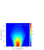
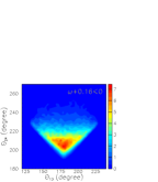
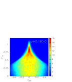
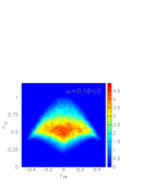
Figure 9: Locations of the $\omega$+0.16$>$0 and respectively $<$0 in the $\theta_{24}$ vs $\theta_{13}$ plane (left panels) and $r_{13}$ vs $r_{24}$ plane (right panels).

However, the criterion used in Figure 7 to define long and short axis quads does not differentiate between them. The two classes are well separated in the $\eta_{S}$ vs $\xi_{S}$ plane but we cannot tell them apart from their location in the $\theta_{24}$ vs $\theta_{13}$ or $r_{13}$ vs $r_{24}$ planes. This illustrates the limitations of using only two parameters in defining a quad configuration. Yet, we know that short axis and long axis quads can be told apart from the different parities of the 1$-$3 image pair: image 3 is inside the critical curve for long axis quads and outside for short axis quads, the opposite being true for the 2$-$4 pair. We translate this property by introducing a parameter $\omega$=$r_{3}-1/2(r_{2}+r_{4})$ which is indeed observed (Figure 8) to be a good discriminant between short-axis and long-axis quads. Its distribution separates the quads in two families, one associated with long axis and the other with short axis configurations. We estimate from Figure 8 (left) that the separation between these occurs approximately at $\omega$$\sim$$-$0.16. However, Figure 9 shows that the two classes overlap in both the $\theta_{24}$ vs $\theta_{13}$ and $r_{13}$ vs $r_{24}$ planes.

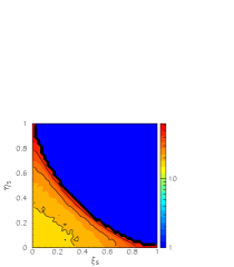
Figure 10: Left: the $\eta_{S}$ vs $\xi_{S}$ distribution of the CASTLeS quad sample as calculated from the ($\theta_{24},\theta_{13}$) and ($r_{24},r_{13}$) pairs (Table 3). The locations of RX J0911 and B2045+265 are evaluated from the $\theta$ pair exclusively (see text). Right: map of the mean total magnification (sum of the absolute values) in the $\eta_{S}$ vs $\xi_{S}$ plane.

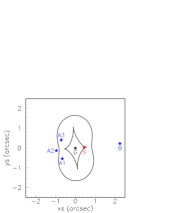
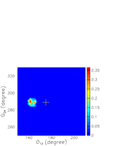
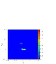
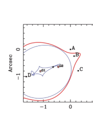
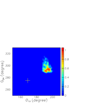
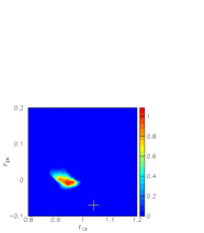
Figure 11: The cases of RXJ 0911 and B2045+265 are illustrated in the upper and lower rows respectively. In each row, from left to right, we display the results of appropriate lens models (Hoai et al. (2013) for RX J0911 and McKean et al. (2007) for B2045+265) and comparisons between prediction and measurement in the $\theta_{24}$ vs $\theta_{13}$ plane and in the $r_{24}$ vs $r_{13}$ plane respectively. Predictions are calculated for $|r_{13}-0.98|$$<$0.02 and $|r_{24}-0.06|$$<$0.02 (RX J0911, $\theta_{24}$ vs $\theta_{13}$); for $|\theta_{24}-289\text{${}^{\circ}$}|$$<$5^∘and $|\theta_{13}-178\text{${}^{\circ}$}|$$<$5^∘(RX J0911, $r_{24}$ vs $r_{13}$); for $|r_{13}-1.04|$$<$0.05 and $|r_{24}+0.07|$$<$0.05 (B2045, $\theta_{24}$ vs $\theta_{13}$); for $|\theta_{24}-275\text{${}^{\circ}$}|$$<$5^∘and $|\theta_{13}-169\text{${}^{\circ}$}|$$<$5^∘ (B2045, $r_{24}$ vs $r_{13}$). Crosses indicate the locations of the measured values.

3.3 Locating the quasar inside the caustic from the image configuration

Table 3: Location of the quasar point source in the lens caustic obtained from the quad configuration and comparison of the associated model prediction with measurement.

	Name	$\xi_{s}$	$Q(\xi_{s})$	$\eta_{s}$	$Q(\eta_{s})$	$Q(x_{L})$	$Q(y_{L})$
1	PMNJ0134-0931	0.02$\pm$0.01	0.01	0.85$\pm$0.02	0.22	$-$	$-$
2	HE0230-2130	0.16$\pm$0.02	0.23	0.30$\pm$0.03	0.45	4.2	4.4
3	MG0414+0534	0.09$\pm$0.02	0.36	0.71$\pm$0.03	0.53	1.9	4.0
4	HE0435-1223	0.03$\pm$0.01	0.16	0.24$\pm$0.02	0.09	0	0.7
5	B0712+472	0.07$\pm$0.02	0.05	0.69$\pm$0.03	0.27	$-$0.4	0.4
6	HS0810+2554	0.12$\pm$0.02	0.55	0.60$\pm$0.03	0.67	2.8	$-$0.9
8	SDSS0924-0219	0.29$\pm$0.03	0.29	0.25$\pm$0.03	0.04	$-$1.9	1.7
9	SDSS1004+4112	0.21$\pm$0.06	0.07	0.49$\pm$0.08	0.09	0.3	$-$1.1
10	SDSS1011+0143	0.06$\pm$0.01	0.66	0.18$\pm$0.02	0.67	0.9	3.9
11	PG1115+080	0.37$\pm$0.04	0.18	0.30$\pm$0.05	0.27	$-$0.6	0.8
12	RXJ1131-1231	0.01$\pm$0.01	0.10	0.82$\pm$0.02	0.33	0.5	$-$0.4
13	SDSS1138+0314	0.16$\pm$0.02	0.25	0.25$\pm$0.02	0.45	$-$0.4	0.8
14	HST12531-2914	0.05$\pm$0.01	0.64	0.33$\pm$0.02	0.14	0.7	0.1
15	HST14113+5211	0.09$\pm$0.02	0.45	0.11$\pm$0.02	0.52	0	$-$2.1
16	H1413+117	0.03$\pm$0.01	0.19	0.18$\pm$0.02	0.66	$-$2.7	0.3
17	HST14176+5226	0.06$\pm$0.01	0.69	0.14$\pm$0.02	0.04	2.2	0
18	B1422+231	0.05$\pm$0.01	0.18	0.70$\pm$0.03	0.45	$-$3.9	0.9
19	B1555+375	0.15$\pm$0.03	0.02	0.58$\pm$0.04	0.07	2.6	0.4
20	WF12026-4536	0.44$\pm$0.04	0.25	0.20$\pm$0.04	0.28	$-$1.8	1.1
21	WF12033-4723	0.34$\pm$0.05	0.14	0.30$\pm$0.05	0.55	$-$0.3	$-$0.6
23	Q2237+030	0.05$\pm$0.01	0.71	0.30$\pm$0.02	0.33	0.2	$-$0.1

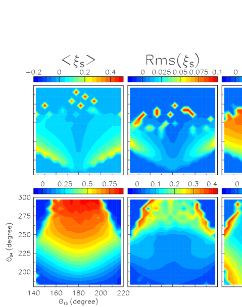
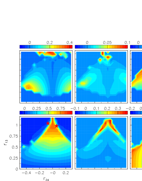
Figure 13: Model maps of the mean values and rms values of $\xi_{S}$ and $\eta_{S}$ calculated for $\sigma_{\gamma}$=0.1, as indicated on top of each column. Rows go by pairs. The upper pair shows maps in the $\theta_{24}$ vs $\theta_{13}$ plane. The lower pair shows maps in the $r_{13}$ vs $r_{24}$ plane. In each pair the upper (lower) row is for $\omega$+0.16 negative (positive).

The results of the previous Section show that it should be possible to evaluate the values of $\xi_{S}$ and $\eta_{S}$ from those of $\theta_{13}$ and $\theta_{24}$ or $r_{13}$ and $r_{24}$. To this end we use the model to produce maps of the mean and rms values of $\xi_{S}$ and $\eta_{S}$ in the $r_{13}$ vs $r_{24}$ and $\theta_{13}$ vs $\theta_{24}$ planes. However, in order to avoid difficulties with the ambiguous cases illustrated in Figure 8, we separate the quads in two families according to the sign of the quantity $\omega$+0.16. The maps of the mean and rms values are displayed in Figure 13 of the Appendix for $\sigma_{\gamma}$=0.1. We then associate to each CASTLeS quad a location in the $\eta_{S}$ vs $\xi_{S}$ plane as obtained from these maps. Precisely, we obtain the mean and rms values of $\xi_{S}$ and $\eta_{S}$ for the $r$ pair and $\theta$ pair independently. Knowing $\theta_{13}$, $\theta_{24}$ and $\omega$, we obtain $<$$\xi_{S}$$>_{\theta}$, $<$$\eta_{S}$$>_{\theta}$, Rms($\xi_{s}$)_θ and Rms($\eta_{s}$)_θ from the appropriate map. Similarly, knowing $r_{13}$, $r_{24}$ and $\omega$, we obtain $<$$\xi_{S}$$>_{r}$, $<$$\eta_{S}$$>_{r}$, Rms($\xi_{s}$)_r and Rms($\eta_{s}$)_r from the appropriate map. We then combine the $r$-pair and $\theta$-pair evaluations as shown below. The result is listed in Table 3 and illustrated in Figure 10. Table 3 lists for each quad the mean values of the coordinates $\xi_{S}$ and $\eta_{S}$ of the source obtained from the ($\theta_{13},\theta_{24}$) and ($r_{13},r_{24}$) pairs, namely:

$$\xi_{S}= \frac{\{<\xi_{S}>_{\theta}/\mbox{Rms}^{2}(\xi_{S})_{\theta}+<\xi_{S}>_{r}/\mbox{Rms}^{2}(\xi_{S})_{r}\}}{1/\mbox{Rms}^{2}(\xi_{S})_{\theta}+1/\mbox{Rms}^{2}(\xi_{S})_{r}}$$

$$\pm\frac{1}{\left\{{1/\mbox{Rms}^{2}(\xi_{S})_{\theta}+1/\mbox{Rms}^{2}(\xi_{S})_{r}}\right\}^{1/2}}$$

Similarly,

$$\eta_{S}= \frac{\{<\eta_{S}>_{\theta}/\mbox{Rms}^{2}(\eta_{S})_{\theta}+<\eta_{S}>_{r}/\mbox{Rms}^{2}(\eta_{S})_{r}\}}{1/\mbox{Rms}^{2}(\eta_{S})_{\theta}+1/\mbox{Rms}^{2}(\eta_{S})_{r}}$$

$$\pm\frac{1}{\left\{{1/\mbox{Rms}^{2}(\eta_{S})_{\theta}+1/\mbox{Rms}^{2}(\eta_{S})_{r}}\right\}^{1/2}}$$

Here, $<$$\xi_{S}$$>_{\theta}$, $<$$\xi_{S}$$>_{r}$, $<$$\eta_{S}$$>_{\theta}$ and $<$$\eta_{S}$$>_{r}$ are the mean values of respectively $\xi_{S}$ and $\eta_{S}$ obtained from the maps of Figure 13 for the $\theta$ and $r$ pair respectively.
Similarly, $\text{Rms}(\xi_{S})_{\theta}$, $\text{Rms}(\xi_{S})_{r}$, $\text{Rms}(\eta_{S})_{\theta}$ and $\text{Rms}(\eta_{S})_{r}$ are the Rms values of respectively $\xi_{S}$ and $\eta_{S}$ obtained from the maps of Figure 13 for the $\theta$ and $r$ pair respectively. For each quad we also list quality factors $Q(\xi_{S})$ and $Q(\eta_{S})$, which measure the agreement between the two evaluations (using the $\theta$ pair or the $r$ pair):

$$Q(\xi_{S})=\left\{\frac{(<\xi_{S}>_{\theta}-\xi_{S})^{2}}{\mbox{Rms}^{2}(\xi_{S})_{\theta}}+\frac{(<\xi_{S}>_{r}-\xi_{S})^{2}}{\mbox{Rms}^{2}(\xi_{S})_{r}}\right\}^{1/2}$$

$$Q(\eta_{S})=\left\{\frac{(<\eta_{S}>_{\theta}-\eta_{S})^{2}}{\mbox{Rms}^{2}(\eta_{S})_{\theta}}+\frac{(<\eta_{S}>_{r}-\eta_{S})^{2}}{\mbox{Rms}^{2}(\eta_{S})_{r}}\right\}^{1/2}$$

The agreement is excellent, with $Q$ values not exceeding 0.7 and having an average of 0.3. In particular, it is remarkable that SDSS1004 (nr 9), in spite of being lensed by a galaxy cluster, is very well described by the simple lens model. The quasar point sources of the CASTLeS quad sample are seen to populate preferably the region close to the caustic boundary, where the magnification is important. This bias is well known. We illustrate it by mapping the mean magnification (in absolute value and summed over the four images) in the $\eta_{S}$ vs $\xi_{S}$ plane for model quads (Figure 10 right).

Figure 12: Distribution of the quality factors $Q(x_{L})$ (left) and $Q(y_{L}$) (right).

Two CASTLeS quads are omitted from Table 3: RX J0911 (nr 7) and B2045+265 (nr 22). Both are short axis quads according to the value of $\omega$. Their values of ($\theta_{13},\theta_{24},r_{13},r_{24}$) are (178^∘, 289^∘, 0.98, 0.06) and (169^∘, 275^∘, 1.04, $-$0.07) respectively, making them, by far, the quads having the largest values of $r_{13}$ and $\theta_{24}$ (see Figures 5 and 6). Their locations on the $r$ pair maps of Figure 13 (fourth row) are very close to the edge of the acceptable region. In such cases the lens equation imposes very strong constraints on the normalised coordinates, as is also visible in Figures 5 and 6. The point $\theta_{13}$=180^∘, $r_{24}$=0 is a centre of symmetry, implying $\theta_{2}$=360^∘$-$ $\theta_{4}$. In its vicinity there is very little room to accommodate quad configurations. The same is true near the upper and lower ends of the $r_{13}$ vs $\theta_{24}$ plot. We illustrate this further in Figure 11, which displays the predicted values of the $r$ pair when the $\theta$ pair is set equal to the measured values and, conversely, the predicted values of the $\theta$ pair when the $r$ pair is set equal to the measured values. In both cases, the two sets are disconnected. This implies that the $r$ pair cannot be used to obtain a reliable evaluation of $\xi_{S}$ and $\eta_{S}$. We show in Figure 10 the evaluations obtained from the $\theta$ pair; however, they are associated with large error bars.

3.4 The lens location: comparison with model prediction

The analyses presented in the preceding sections are independent of the location of the lens. They do not require that it be observed. In order to study the additional information that such an observation provides, we call $x_{L}$ and $y_{L}$ the lens normalised coordinates, obtained from the measured values by applying the same coordinate transformation as for the images. Those of the CASTLeS quad sample are listed in Table 1 and compared with model prediction in the right panel of Figure 5. Note that changing the sign of $y_{L}$ leaves the configuration invariant: we can only hope to measure $|y_{L}|$. In order to assess the ability of the model to predict the location of the lens, we calculate for each CASTLeS quad the values of $x_{L}$ and $|y_{L}|$ predicted by the model when $\xi_{S}$ and $\eta_{S}$ take the values listed in Table 3. More precisely, we calculate their distributions when $\xi_{S}$ and $\eta_{S}$ are Gaussian distributed about these values with the associated dispersions listed in Table 3. We call $<$$x_{L}$$>$^∗ and $<$$|y_{L}|$$>$^∗ the means of these distributions and $\text{Rms}^{*}(x_{L})$ and $\text{Rms}^{*}(|y_{L}|)$ their rms values. We compare these model predictions to the measured values $x_{L}$ and $|y_{L}|$ listed in Table 1 by defining two quality factors, $Q(x_{L})=(x_{L}-$$<$$x_{L}$$>$${}^{*})$/$\Delta(x_{L})$ and $Q(y_{L})=(|y_{L}|-$$<$$|y_{L}|$$>^{*})$/$\Delta(|y_{L}|)$ where $\Delta(x_{L})$ and $\Delta(|y_{L}|)$ are obtained by summing in quadrature an estimated measurement error of 0.02 with $\text{Rms}^{*}(x_{L})$ and $\text{Rms}^{*}(|y_{L}|)$ respectively. Their distributions are displayed in Figure 12. The mean$\pm$rms values are 0.3$\pm$1.9 and $-$0.2$\pm$1.8 respectively. A quad is omitted from Figure 12: PMNJ0134$-$0931 (nr 1), a quasar for which the CASTLeS assignment of the lens is not reliable (Winn et al., 2002; Wiklind et al., 2018). The other cases show qualitative agreement between measurement and model prediction, however nearly twice worse than predicted.

4 SUMMARY

In line with the work of previous authors who gave evidence for simple considerations on the image configuration to offer ample information on the lensing mechanism without having recourse to a detailed modelling of the lensing potential, we have given a further illustration of such remarkable properties of gravitational optics. The introduction of normalised coordinates aimed at defining quad configurations independently from location, orientation and size has revealed the presence of strong correlations specific to the gravitational lensing mechanism. These are conveniently expressed as correlations between the opening angle of a pair of images of given parity and the radial difference of the pair of opposite parity. As a result a quad configuration can be approximately described by a pair of parameters: the $\theta$ pair, giving the values of the opening angles of the odd and even pairs of images, or the $r$ pair, giving the values of their radial differences. Such description does not require the lens to be detected.

We have applied these considerations to the study of a sample of HST quads collected by the CASTLeS collaboration and we have shown how the location of the quasar point source within the lens caustic can be evaluated from the quad configuration. The agreement between the results obtained using the $\theta$ pair and the $r$ pair has given confidence in the validity of the description of the lensing mechanism by a very simple lens model. This model has a single parameter, the amplitude of the external shear, and the results that have been obtained display very little dependence on its precise value.

The study has shown the soundness of the classification proposed by Saha & Williams (2003) and quantified the relation that it implies between quad configuration and source location within the lens caustic. The special case of quads having the odd parity images and the lens nearly aligned has been given special attention and the constraints imposed on their normalised coordinates, related to symmetry with respect to the line on which the lens and the odd parity images are located, have been commented upon. The distinction between long-axis and short-axis quads, which becomes trivially meaningless when the shear term, $\gamma$, cancels, has been found to be difficult to handle. We have introduced an ad hoc parameter, $\omega$, to this effect, constructed from a well known property of quad systems.

The CASTLeS quad sample has been shown to be biased toward high magnification images, a result that is well known. Our definition of normalised coordinates does not require the lens to be observed but, when available, the measured normalised coordinates of the lens centre have been found in general agreement with model predictions.

Image magnifications have not been discussed in the present article. They are the subject of many detailed studies triggered by the anomalies that are often observed, calling for appropriate interpretations (see for example Keeton et al. (2003, 2005) and references therein). Addressing such questions is well beyond the scope of the present work; however, we note that the two cases that were singled out in the present study, RXJ 0911 and B2045+265, are part of the sample of anomalous flux quads identified by Keeton et al. (2003, 2005). But this is probably pure coincidence, the other members of the anomalous flux sample being evenly distributed among the CASTLeS quads.

In conclusion, this study has offered an interesting exploration of the general properties of quadruply imaged quasars and has deepened our understanding of the lensing mechanism at stake. However, its ambitions cannot reach further than that. A serious and reliable study of gravitationally lensed images implies the construction of an appropriate lens potential and the resolution of the associated lens equation, which nothing can replace.

Appendix A

References

- Blandford et al. (1989) Blandford R.D., Kochanek C.S., Kovner I. and Narayan R., 1989, Gravitational Lens Optics, Science 245, 824.
- (2) CASTLES https://cfa.harvard.edu/castles/
- Falco et al. (1999) Falco E.E., Kochanek. C.S., Lehar J., McLeod B.A., Munoz J.A., Impey C.D., Keeton C.R., Peng C.Y., & Rix H.-W., 1999, The CASTLES gravitational lensing tool, astro-ph/9910025.
- Hoai et al. (2013) Hoai D.T., Nhung P.T., Anh P.T. et al., 2013, Gravitationally lensed extended sources: the case of QSO RXJ0911, RAA 13(7) 803.
- Kassiola & Kovner (1995) Kassiola, A. & Kovner, I., 1995, Invariants of simple gravitational lenses, MNRAS, 272, 363.
- Keeton et al. (2003) Keeton C.R., Gaudi B.S. and Petters A.O., 2003, Identifying Lenses with Small-Scale Structure. I. Cusp Lenses, ApJ, 598, 138.
- Keeton et al. (2005) Keeton C.R., Gaudi B.S. and Petters A.O., 2005, Identifying Lenses with Small-Scale Structure. II. Fold Lenses, ApJ, 635, 35.
- Kovner (1987) Kovner, I., 1987, The Quadrupole Gravitational Lens, ApJ, 312, 22.
- McKean et al. (2007) McKean J.P., Koopmans L.V.E., Flack C.E. et al., 2007, High-resolution imaging of the anomalous flux ratio gravitational lens system CLASS B2045+265: dark or luminous satellites?, MNRAS, 378, 109.
- Oguri et al. (2004) Oguri M., Inada N., Keeton C.R. et al., 2004, Observations and Theoretical Implications of the Large-Separation Lensed Quasar SDSS J1004+4112, ApJ, 605, 78.
- Saha & Williams (2003) Saha P. & Williams L.L.R., 2003, Qualitative Theory for Lensed QSOs, A.J., 125, 2769.
- Schechter & Wynne (2019) Schechter,P.L. and Wynne, R.A., 2019, Even Simpler Modeling of Quadruply Lensed Quasars (and Random Quartets) Using Witt’s Hyperbola, ApJ, 876, 9.
- Wiklind et al. (2018) Wiklind T., Combes F. and Kanekar N., 2018, ALMA Observations of Molecular Absorption in the Gravitational Lens PMN 0134-0931 at z = 0.7645, ApJ, 864, 73.
- Winn et al. (2002) Winn J.N., Lovell J.E.J. et al., 2002, PMN J0134-0931: A Gravitationally Lensed Quasar with Unusual Radio Morphology, ApJ, 564, 143.
- Witt (1996) Witt, H. J., 1996, Using Quadruple Lenses to Probe the Structure of the Lensing Galaxy, ApJ, 472, L1.
- Woldesenbet & Williams (2012) Woldesenbet, A.G. and Williams, L.L.R., 2012, The Fundamental Surface of quad lenses, MNRAS, 420, 2944.