• We consider the longitudinal dynamical two-point function of the XXZ quantum spin chain in the antiferromagnetic massive regime. It has a series representation based on the form factors of the quantum transfer matrix of the model. The $n$th summand of the series is a multiple integral accounting for all $n$-particle $n$-hole excitations of the quantum transfer matrix. In previous works the expressions for the form factor amplitudes appearing under the integrals were either again represented as multiple integrals or in terms of Fredholm determinants. Here we obtain a representation which reduces, in the zero-temperature limit, essentially to a product of two determinants of finite matrices whose entries are known special functions. This will facilitate the further analysis of the correlation function.

1 Introduction

In this work we renew our attempts to obtain simple and manageable expressions for the dynamical correlation functions of the XXZ chain. The XXZ chain is an anisotropic deformation of the Heisenberg chain which is the fundamental model of 1d magnetism. The XXZ Hamiltonian for a chain of length $L$ acts on the tensor product ${\cal H}_{L}=\bigotimes_{j=1}^{L}V_{j}$, $V_{j}={\mathbb{C}}^{2}$, in which every factor is identified with a site in a 1d lattice. It is defined by

$$H_{L}=J\sum_{j=1}^{L}\Bigl{\{}\sigma_{j-1}^{x}\sigma_{j}^{x}+\sigma_{j-1}^{y}\sigma_{j}^{y}+\Delta\bigl{(}\sigma_{j-1}^{z}\sigma_{j}^{z}-1\bigr{)}\Bigr{\}}-\frac{h}{2}\sum_{j=1}^{L}\sigma_{j}^{z}\,,$$ (1)

where $\sigma^{\alpha}\in\operatorname{End}{\mathbb{C}}^{2}$, $\alpha=x,y,z$, are the Pauli matrices. The three real parameters of the Hamiltonian are the anisotropy $\Delta$, the exchange interaction $J>0$, and the strength $h>0$ of an external magnetic field in the direction of the magnetic symmetry axis.

If the magnet is in contact with a heat bath of temperature $T$, it is in a ‘mixed state’ with canonical density matrix

$$\rho_{L}(T)=\frac{\operatorname{e}^{-H_{L}/T}}{\operatorname{tr}\{\operatorname{e}^{-H_{L}/T}\}}\,.$$ (2)

The Heisenberg time evolution of a local operator $x_{j}\in\operatorname{End}V_{j}$ is defined by

$$x_{j}\mapsto x_{j}(t)=\operatorname{e}^{{\rm i}H_{L}t}x_{j}\operatorname{e}^{-{\rm i}H_{L}t}\,.$$ (3)

A typical quantity measured in experiments on quasi-1d magnets is the dynamical two-point correlation function

$$\bigl{\langle}x_{j}y_{k}(t)\bigr{\rangle}_{T}=\lim_{L\rightarrow\infty}\operatorname{tr}\bigl{\{}\rho_{L}(T)x_{j}y_{k}(t)\bigr{\}}\,.$$ (4)

of two local operators $x_{j}$, $y_{k}$.

The analysis of finite-temperature dynamical correlation functions such as (4) is rather involved. Even for integrable lattice models like the XXZ chain very little is known in the general finite temperature case. Notable exceptions are so-called free-fermion models as, for instance, the XX chain (Hamiltonian (1) with $\Delta=0$) [32, 13, 34, 25, 26, 27] or the transverse field Ising model [28, 30, 31], where much of the long-time large-distance asymptotics was worked out and numerically efficient representations of the correlation functions are available.

In the low-temperature limit, $T\rightarrow 0$, when $\rho_{L}(T)$ becomes proportional to the projector onto the groundstate subspace, the dynamical correlation functions of the XXZ chain are better understood. They were mainly analysed by means of form factor series expansions based on matrix elements of local operators between the ground state and the excited states of the Hamiltonian. The ground state phase diagram is depicted in Figure 1.

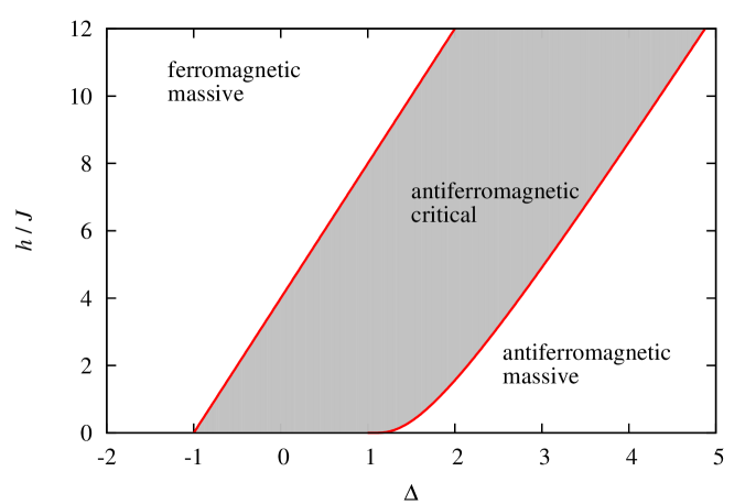
Figure 1: The ground state phase diagram of the XXZ chain in the $\Delta$-$h/J$ plane. The ferromagnetic massive regime and the antiferromagnetic critical regime are separated by the upper critical field $h_{u}=4J(1+\Delta)$ (left red line). The lower critical field $h_{\ell}$ (right red line, defined in equation (54) below) determines the border between the antiferromagnetic critical and the antiferromagnetic massive regime.

The analysis focused on the antiferromagnetic regions of the phase diagram. Form factors for the antiferromagnetic massive regime were first obtained within the $q$-vertex operator approach by Jimbo and Miwa [35]. In this approach the form factors are obtained in the form of multiple integrals which are interpreted in terms of even-numbered multiple-spinon excitations and are called the $2n$-spinon form factors. Since only the two-spinon form factors are known explicitly in terms of special functions, most of the subsequent analysis focused on the two-spinon contribution to the dynamical correlation functions. Moreover, the emphasis was on the calculation of the spatial and temporal Fourier transforms of the dynamical two-point functions, the so-called ‘dynamical structure factors,’ since these are the functions that are measured more or less directly in neutron scattering experiments on certain quasi one-dimensional magnets. The two-spinon dynamical structure factor of the XXZ chain in the antiferromagnetic massive regime was studied in [7, 8, 12, 55]. The important limiting case of the XXX chain (Hamiltonian (1) with $\Delta=1$) was considered in [38]. The four-spinon contribution for the XXX model was calculated in [9]. Two- and four spinon contributions together seem to give a rather quantitative description of the available experimental data [54]. The space-time asymptotics of the longitudinal dynamical two-point functions of the XXZ chain in the antiferromagnetic massive regime was analysed in [17].

The $q$-vertex operator approach is designed to work directly in the thermodynamic limit. Unfortunately, so far it has been successful only for massive integrable models and only for the case of vanishing magnetic field. The two-spinon contribution to the dynamical structure factor of the XXZ chain in the antiferromagnetic massless regime at vanishing magnetic field was obtained in [10] using expressions for the two-spinon form factors of the XYZ chain [53] and performing a massless limit. For the exploration of higher-spinon contributions or of the antiferromagnetic massless phase at non-zero magnetic field the available results on dynamical correlation functions rely on Bethe Ansatz techniques.

An efficient Bethe Ansatz approach to the calculation of form factors of the finite XXZ chain was developed in [44]. Such an approach has the advantage that is applies equally well to all points in the ground state phase diagram. However, the calculation of the thermodynamic limit of the form factors in the general situation is rather sophisticated [60, 33, 39, 41, 16, 47, 43]. The summation of the form factor series imposed additional difficulties that were overcome in [40, 42, 16, 49].

In [44] the form factors pertaining to the finite XXZ chain of even length $L$ were obtained in a form proportional to determinants of matrices of size $N\times N$ with $N$ growing in $L$. These were analysed quite successfully by solving the Bethe Ansatz equations numerically [4] and resulted in predictions for the dynamical structure factors in finite magnetic fields [58, 11] that could be compared with experiments. In the thermodynamic limit, $L\rightarrow\infty$, the $N\times N$ determinants, generically, turn into Fredholm determinants of integral operators [39, 41]. For a long time the Fredholm determinant corresponding to Baxter’s staggered polarisation [1, 2], i.e. the Fredholm determinant arising in the calculation of the matrix element of $\sigma^{z}$ between the two asymptotically degenerate groundstates of the XXZ chain in the antiferromagnetic massive regime of the XXZ chain, was the only known example that could be evaluated more explicitly in terms of known special functions [33]. Only recently the well-known explicit result for the two-spinon form factors of the XXX chain [35] was reproduced from an algebraic Bethe Ansatz perspective [43].

Altogether the thermodynamic limit of the form factors generally results in rather technical expressions which can be seen as multiple residues related to the zeros of the counting functions of the massive excitations in the respective ground state regimes [16, 49]. In spite of the technically complicated nature of the expressions for the form factors, the series derived in [49] could be used for a detailed analysis of the space-time asymptotics of the dynamical two-point functions of the XXZ chain in the antiferromagnetic massless regime at finite magnetic field [50] and of the threshold singularities of their Fourier transforms [48]. This analysis confirmed and refined, from a microscopic point of view, the non-linear Luttinger liquid phenomenology (for a review see [29]).

An alternative route to the zero temperature correlation functions of the XXZ chain is through the thermal form factor expansion [14, 18] developed initially for static correlation functions and later extended to the dynamical case in [22]. The thermal form factor expansion is an expansion involving the form factors and eigenvalues of the quantum transfer matrix. The latter is an auxiliary object originally introduced [64, 63, 46] in order to study the thermodynamics of quantum spin chains. The quantum transfer matrix is generically non-Hermitian. Its eigenvalues are not necessarily all real. The eigenvalue of largest modulus, however, is always real and non-degenerate (which was rigorously established for temperature high enough in [21]). We call it the dominant eigenvalue and the corresponding eigenvector the dominant eigenvector. The dominant eigenvector determines the reduced density matrices of all finite sub-segments of the considered quantum spin chain in the thermodynamic limit [23, 24]. Dynamical correlation functions can be expressed as form factor series involving the matrix elements of the operators of the algebraic Bethe Ansatz between the dominant state and excited states of the quantum transfer matrix [22].

The spectrum and the Bethe roots of the quantum transfer matrix of an integrable quantum spin chain are rather different from the spectrum and Bethe roots of the ordinary transfer matrix associated with the Hamiltonian. Both depend parametrically on the temperature and, in case of the XXZ chain, on the external magnetic field. The Bethe roots form patterns in the complex plane which ‘evolve’ with increasing temperature. These patterns are currently not sufficiently well understood to allow for an analysis of the thermal form factor series of the dynamical two-point functions of the XXZ chain at arbitrary temperatures. For this reason we shall focus in this work on the case of the low-temperature limit of the XXZ chain in the antiferromagnetic massive regime, which is the only parameter regime so far, where we have obtained a complete picture of all excitations and explicit expressions for all eigenvalues [15]. Amazingly, the corresponding Bethe root patterns are much simpler than those belonging to the excited states of the Hamiltonian in the same regime of the ground state phase diagram. They are characterized by the absence of so-called strings. Accordingly, they also come with a different interpretation. While the excitations of the Hamiltonian are interpreted in terms of spinons (see e.g. [16]), the excitations of the quantum transfer matrix are parameterised by Bethe root patterns of particle-hole type. In the zero temperature limit every excitation is determined by two finite sets of complex parameters, called particle- and hole roots, and by a ‘topological index’ $k\in{\mathbb{Z}}/2{\mathbb{Z}}$. The particle- and hole roots are confined on two simple finite curves in the upper and lower half plane, respectively, which are symmetric with respect to reflection about the real and imaginary axis (see Figure 2).

In [14] we found that the amplitudes in the form factor expansions factorize in three parts which we called the universal part, the factorizing part and the determinant part. In the so-called Trotter limit, which is a necessary step of the formalism, the universal and factorising parts were taking a very explicit form given in terms of exponents of one and two dimensional integrals. In the low-T limit, we showed that all these quantities can be evaluated in closed form in terms of products of $q$-gamma and $q$-Barnes functions. In its turn, the determinant part was represented as a ratio of two Fredholm determinants in the numerator over two Fredholm determinants in the denominator. While in the low-T limit the Fredholm determinants in the denominator turned out to be explicitly computable in terms of $q$-products the Fredholm determinants in the numerator had too complicated kernels so as to go beyond the Fredholm determinant representation. This was not much of a problem for the numerical evaluation of the correlation functions through its thermal form factor expansions. However, this structural intricacy of the integrands in the form factor expansion raised doubts about the usefulness of the representation for an analytic study of other properties of the correlation functions, such as their long-distance and large-time asymptotic behaviour.

By relying on a form of determinant factorisation proposed in [43], we obtain in this work a representation for the amplitudes arising in the thermal form factor expansion of the generating function of the dynamical longitudinal correlation functions. The latter is structured in such a way that, in the low-$T$ limit, the full amplitudes become explicitly computable in terms of products of $q$-gamma and $q$-Barnes functions and finite size determinants built up of $q$-gamma and theta functions. These expressions for the form factors are then used to express the dynamical two-point function $\langle\sigma_{1}^{z}\sigma_{m+1}^{z}(t)\rangle_{T=0}$ as a novel series of multiple integrals with very explicit and simple integrands. More precisely we shall derive the following

Theorem.

The longitudinal dynamical two-point function of the XXZ chain in the antiferromagnetic massive regime and in the zero-temperature limit can be expressed in terms of a generating function ${\cal G}^{(0)}$,

$$\bigl{\langle}\sigma_{1}^{z}\sigma_{m+1}^{z}(t)\bigr{\rangle}={\textstyle\frac{1}{2}}\partial_{\gamma\alpha}^{2}D_{m}^{2}{\cal G}^{(0)}(m+1,t,\alpha)\bigr{|}_{\alpha=0}\,.$$ (5)

Here $\gamma$ parameterizes the anisotropy $\Delta=\operatorname{ch}(\gamma)$ and $D_{m}$ denotes the difference operator, formally defined by $D_{m}f_{m}=f_{m}-f_{m-1}$. The generating function has a series representation of the form

$${\cal G}^{(0)}(m,t,\alpha)=\frac{\vartheta_{2}^{2}({\rm i}\gamma\alpha/2)}{\vartheta_{2}^{2}}+\frac{\vartheta_{1}^{2}({\rm i}\gamma\alpha/2)}{\vartheta_{2}^{2}}(-1)^{m}\\[4.30554pt] +\sum_{\begin{subarray}{c}\ell\in{\mathbb{N}}\\ k=0,1\end{subarray}}\frac{(-1)^{km}}{(\ell!)^{2}}\int_{{\cal C}_{h}^{\ell}}\frac{{\rm d}^{\ell}u}{(2\pi{\rm i})^{\ell}}\int_{{\cal C}_{p}^{\ell}}\frac{{\rm d}^{\ell}v}{(2\pi{\rm i})^{\ell}}\>{\cal A}({\cal U},{\cal V}|k)\operatorname{e}^{-{\rm i}\sum_{\lambda\in{\cal U}\ominus{\cal V}}(mp(\lambda)+t\varepsilon(\lambda|h))}\,,$$ (6)

where $\vartheta_{1}$ and $\vartheta_{2}$ are Jacobi theta functions, where $p$ and $\varepsilon$ are the dressed momentum and dressed energy of the excitations, and where the form factor amplitudes are given by

$${\cal A}({\cal U},{\cal V}|k)=\frac{\vartheta_{2}^{2}(\Sigma_{0}({\cal U},{\cal V}))}{\vartheta_{2}^{2}}\biggl{[}\prod_{\lambda,\mu\in{\cal U}\ominus{\cal V}}\mspace{-18.0mu}\Psi(\lambda-\mu)\biggr{]}\\ \times\det_{\ell}\{\Omega(u_{j},v_{k}|{\cal U},{\cal V})\}\det_{\ell}\{\overline{\Omega}(v_{j},u_{k}|{\cal U},{\cal V})\}\,.$$ (7)

The sets ${\cal U}=\{u_{j}\}_{j=1}^{\ell}$, ${\cal V}=\{v_{j}\}_{j=1}^{\ell}$ gather all integration variables. The contours ${\cal C}_{h}$ and ${\cal C}_{p}$ are intervals $[-\pi/2,\pi/2]$ shifted down or up in the complex plane (cf. (224)). The notation $\sum_{\lambda\in{\cal U}\ominus{\cal V}}$ means that summands indexed by elements of ${\cal U}$ come with a plus sign, while summands indexed by elements of ${\cal V}$ get a minus sign (for a formal definition see (52) below). The remaining functions $\Sigma_{0}$, $\Psi$ and $\Omega$ are explicitly defined in terms of theta, $q$-gamma and $q$-Barnes functions. Their precise definition will be given in equations (183), (216) and (206) in the main body of the text. $\Sigma_{0}$ and the functions $\Omega$ and $\overline{\Omega}$ depend parametrically on the ‘twist parameter’ $\alpha$.

This work is organised as follows. In Section 2 we recall the results of [22] on the thermal form-factor series representation of dynamical correlation functions. Section 3 contains a review of the low-$T$ analysis of the spectrum and Bethe root patterns of the quantum transfer matrix of the XXZ chain in the antiferromagnetic massive regime obtained in [15]. We also provide appropriate forms of non-linear integral equations that will be needed in the sequel. Section 4 contains the main technical part of this work, a low-$T$ analysis of the amplitudes in the thermal form factor series. The new form of the amplitudes is then used in Section 5 in order to obtain our novel form factor series expansion of the longitudinal two-point function. We also discuss the explicit evaluation of the remaining finite determinants in terms of basic hypergeometric series. Section 6 is devoted to the isotropic limit, and Section 7 to some conclusions of this work. A few supplementary technical details are deferred to two appendices.

2 The thermal form factor series

In previous work [22] we have developed a thermal form factor approach to dynamical correlation functions of Yang-Baxter integrable models. It is based on a ‘vertex-model representation’ of the canonical density matrix and the time evolution operator [57]. In the following we shall apply this approach to the longitudinal two-point function of the XXZ chain in the antiferromagnetic massive regime in the low-temperature limit.

2.1 The dynamical quantum transfer matrix

The basic object in this approach is a ‘dynamical quantum transfer matrix’ which can be associated with any fundamental solution of the Yang-Baxter equation. For the XXZ chain in the antiferromagnetic massive regime we use the parametrization

$$\begin{array}[]{cc}R(\lambda,\mu)=\begin{pmatrix}1&0&0&0\\ 0&b(\lambda,\mu)&c(\lambda,\mu)&0\\ 0&c(\lambda,\mu)&b(\lambda,\mu)&0\\ 0&0&0&1\end{pmatrix}\,,&\begin{array}[]{c}b(\lambda,\mu)=\frac{\sin(\mu-\lambda)}{\sin(\mu-\lambda+{\rm i}\gamma)}\\[8.61108pt] c(\lambda,\mu)=\frac{\sin({\rm i}\gamma)}{\sin(\mu-\lambda+{\rm i}\gamma)}\end{array}\end{array}\,.$$ (8)

of the $R$-matrix. Here $\gamma>0$, and we set $q=\operatorname{e}^{-\gamma}$ for later convenience.

We define a staggered, twisted and inhomogeneous monodromy matrix acting on ‘vertical spaces’ with ‘site indices’ $1,\dots,2N+2$, and on a ‘horizontal auxiliary space’ indexed $a$,

$$T_{a}(\lambda|h)=\operatorname{e}^{h\sigma_{a}^{z}/2T}R_{2N+2,a}^{t_{1}}(\xi_{2N+2},\lambda+{\rm i}\gamma/2)R_{a,2N+1}(\lambda+{\rm i}\gamma/2,\xi_{2N+1})\\[4.30554pt] \times\dots\times R_{2,a}^{t_{1}}(\xi_{2},\lambda)R_{a,1}(\lambda+{\rm i}\gamma/2,\xi_{1})\,.$$ (9)

The number $N$ will be called the Trotter number. The superscript $t_{1}$ denotes transposition with respect to the first space $R$ is acting on, and $\xi_{1},\dots,\xi_{2N+2}$ are $2N+2$ complex ‘inhomogeneity parameters’. Following [22, 57] we fix these parameters to the values

$$\xi_{2k-1}=-\xi_{2k}=\begin{cases}-\frac{{\rm i}t}{\kappa N}&k=1,\dots,\frac{N}{2}\\[2.15277pt] \varepsilon&k=\frac{N}{2}+1\\[4.30554pt] \frac{{\rm i}t+1/T}{\kappa N}&k=\frac{N}{2}+2,\dots,N+1\,,\end{cases}$$ (10)

where

$$1/\kappa=-2{\rm i}J\operatorname{sh}(\gamma)\,.$$ (11)

The corresponding transfer matrix

$$t(\lambda|h)=\operatorname{tr}_{a}\{T_{a}(\lambda|h)\}$$ (12)

is then what we call a dynamical quantum transfer matrix of the XXZ chain. As we have demonstrated in [22] the dynamical two-point functions of the XXZ chain can be written as a series involving the eigenvalues and form factors of the dynamical quantum transfer matrix. This series will be the starting point of our actual considerations. In order to define it we have to briefly review the algebraic Bethe Ansatz construction of the eigenvectors and eigenvalues of $t(\lambda|h)$.

2.2 Eigenvectors and eigenvalues

The monodromy matrix (9) fulfills the two prerequisites for an algebraic Bethe Ansatz. It satisfies the Yang-Baxter algebra relations

$$R_{ab}(\lambda,\mu)T_{a}(\lambda|h)T_{b}(\mu|h)=T_{b}(\mu|h)T_{a}(\lambda|h)R_{ab}(\lambda,\mu)$$ (13)

by construction, and it has a pseudo vacuum state

$$|0\rangle=\bigl{[}{\textstyle\binom{1}{0}\otimes\binom{0}{1}}\bigr{]}^{\otimes(N+1)}$$ (14)

on which its action is triangular. More precisely, setting

$$T_{a}(\lambda|h)=\begin{pmatrix}A(\lambda|h)&B(\lambda|h)\\ C(\lambda|h)&D(\lambda|h)\end{pmatrix}_{a}\,,$$ (15)

it is not difficult to see that

$$C(\lambda|h)|0\rangle=0\,,\quad A(\lambda|h)|0\rangle=a(\lambda|h)|0\rangle\,,\quad D(\lambda|h)|0\rangle=d(\lambda|h)|0\rangle\,,$$ (16)

where $a(\lambda|h)$ and $d(\lambda|h)$ are the pseudo vacuum expectation values

$$a(\lambda|h) =\operatorname{e}^{\frac{h}{2T}}\frac{\sin\bigl{(}\lambda+\frac{{\rm i}\gamma}{2}+\varepsilon\bigr{)}}{\sin\bigl{(}\lambda+\frac{3{\rm i}\gamma}{2}+\varepsilon\bigr{)}}\Biggl{[}\frac{\sin\bigl{(}\lambda+\frac{{\rm i}\gamma}{2}-\frac{{\rm i}t}{\kappa N}\bigr{)}}{\sin\bigl{(}\lambda+\frac{3{\rm i}\gamma}{2}-\frac{{\rm i}t}{\kappa N}\bigr{)}}\frac{\sin\bigl{(}\lambda+\frac{{\rm i}\gamma}{2}+\frac{{\rm i}t+1/T}{\kappa N}\bigr{)}}{\sin\bigl{(}\lambda+\frac{3{\rm i}\gamma}{2}+\frac{{\rm i}t+1/T}{\kappa N}\bigr{)}}\Biggr{]}^{\frac{N}{2}},$$

$$d(\lambda|h) =\operatorname{e}^{-\frac{h}{2T}}\frac{\sin\bigl{(}\lambda+\frac{{\rm i}\gamma}{2}-\varepsilon\bigr{)}}{\sin\bigl{(}\lambda-\frac{{\rm i}\gamma}{2}-\varepsilon\bigr{)}}\Biggl{[}\frac{\sin\bigl{(}\lambda+\frac{{\rm i}\gamma}{2}+\frac{{\rm i}t}{\kappa N}\bigr{)}}{\sin\bigl{(}\lambda-\frac{{\rm i}\gamma}{2}+\frac{{\rm i}t}{\kappa N}\bigr{)}}\frac{\sin\bigl{(}\lambda+\frac{{\rm i}\gamma}{2}-\frac{{\rm i}t+1/T}{\kappa N}\bigr{)}}{\sin\bigl{(}\lambda-\frac{{\rm i}\gamma}{2}-\frac{{\rm i}t+1/T}{\kappa N}\bigr{)}}\Biggr{]}^{\frac{N}{2}}.$$ (17)

The eigenvalues and eigenstates of the quantum transfer matrix can be parameterized by sets of Bethe roots. These are defined with the aid of an auxiliary function

$$\mathfrak{a}\bigl{(}\lambda\big{|}\{\lambda_{k}\}_{k=1}^{M},h\bigr{)}=\frac{d(\lambda|h)}{a(\lambda|h)}\prod_{k=1}^{M}\frac{\sin(\lambda-\lambda_{k}-{\rm i}\gamma)}{\sin(\lambda-\lambda_{k}+{\rm i}\gamma)}$$ (18)

as the solutions of the ‘Bethe Ansatz equations’

$$\mathfrak{a}\bigl{(}\lambda_{j}\big{|}\{\lambda_{k}\}_{k=1}^{M},h\bigr{)}=-1\,,\quad j=1,\dots,M\,.$$ (19)

Note that the Bethe roots depend parametrically on $t$, $T$, $\gamma$ and $h$. In order to simplify our notation we number the solutions consecutively as $\{\lambda_{j}^{(n)}\}_{j=1}^{M_{n}}$ and denote the corresponding auxiliary functions by

$$\mathfrak{a}_{n}(\lambda|h)=\mathfrak{a}\bigl{(}\lambda\big{|}\{\lambda_{k}^{(n)}\}_{k=1}^{M_{n}},h\bigr{)}\,.$$ (20)

Left and right eigenvectors of the quantum transfer matrix can be constructed from left and right ‘off-shell Bethe vectors’ which, for a given subset $\{\nu\}=\{\nu_{j}\}_{j=1}^{M}\subset{\mathbb{C}}$, are defined as

$$\bigl{\langle}\{\nu\},h\bigr{|}=\langle 0|C(\nu_{1}|h)\dots C(\nu_{M}|h)\,,\quad\bigl{|}\{\nu\},h\bigr{\rangle}=B(\nu_{M}|h)\dots B(\nu_{1}|h)|0\rangle\,.$$ (21)

If $\{\lambda_{j}^{(n)}\}_{j=1}^{M_{n}}$ is a solution of the Bethe Ansatz equations (19), then

$$\langle n,h|=\bigl{\langle}\{\lambda_{j}^{(n)}\}_{j=1}^{M_{n}},h\bigr{|}\,,\quad|n,h\rangle=\bigl{|}\{\lambda_{j}^{(n)}\}_{j=1}^{M_{n}},h\bigr{\rangle}$$ (22)

are left and right eigenvectors of the quantum transfer matrix satisfying

$$\langle n,h|t(\lambda|h)=\langle n,h|\Lambda_{n}(\lambda|h)\,,\quad t(\lambda|h)|n,h\rangle=\Lambda_{n}(\lambda|h)|n,h\rangle\,,$$ (23)

where

$$\Lambda_{n}(\lambda|h)=\bigl{(}1+\mathfrak{a}_{n}(\lambda|h)\bigr{)}a(\lambda|h)\prod_{j=1}^{M_{n}}\frac{\sin\bigl{(}\lambda-\lambda_{j}^{(n)}+{\rm i}\gamma\bigr{)}}{\sin\bigl{(}\lambda-\lambda_{j}^{(n)}\bigr{)}}$$ (24)

is the eigenvalue function.

There is a unique so-called dominant eigenvalue $\Lambda_{0}$, say, which is real and maximal in the sense that $\Lambda_{0}(-{\rm i}\gamma/2|h)>|\Lambda_{n}(-{\rm i}\gamma/2|h)|$ for all $n>0$. We know that $M_{0}=N+1$. To further simplify the notation we drop the index ‘$0$’ for the dominant state, such that $\Lambda=\Lambda_{0}$, $M=M_{0}$, $|h\rangle=|0,h\rangle$, $\mathfrak{a}(\cdot|h)=\mathfrak{a}_{0}(\cdot|h)$, and $\{\lambda_{j}\}_{j=1}^{M}=\{\lambda_{j}^{(0)}\}_{j=1}^{M_{0}}$.

2.3 The thermal form factor series

Let

$$\Sigma^{z}(\lambda|h)=\operatorname{tr}_{a}\{\sigma_{a}^{z}T_{a}(\lambda|h)\}=2T\partial_{h}t(\lambda|h)$$ (25)

and

$$\rho_{n}(\lambda|h,h^{\prime})=\Lambda_{n}(\lambda|h^{\prime})/\Lambda(\lambda|h)\,.$$ (26)

Here and hereafter we keep the magnetic fields $h$ pertaining to the dominant state and $h^{\prime}$ pertaining to the $n$th excited state as independent parameters. This is a common trick that will allow us to introduce a generating function of the longitudinal two-point function. In the end of our calculation in Section 5 we shall see that this generating function depends only on a ‘twist parameter’

$$\alpha=(h-h^{\prime})/(2\gamma T)$$ (27)

which is introduced here for later convenience. It becomes an independent variable in the zero-temperature limit.

Then, according to Theorem 1 of [22],

$$\bigl{\langle}\sigma_{1}^{z}\sigma_{m+1}^{z}(t)\bigr{\rangle}_{T}=\lim_{N\rightarrow\infty}\lim_{\varepsilon\rightarrow 0}\sum_{n}\frac{\langle h|\Sigma^{z}(-{\rm i}\gamma/2|h)|n,h\rangle\langle n,h|\Sigma^{z}(-{\rm i}\gamma/2|h)|h\rangle}{\Lambda_{n}(-{\rm i}\gamma/2|h)\langle h|h\rangle\Lambda(-{\rm i}\gamma/2|h)\langle n,h|n,h\rangle}\\[-4.30554pt] \times\rho_{n}(-{\rm i}\gamma/2|h,h)^{m}\biggl{(}\frac{\rho_{n}(-{\rm i}\gamma/2+{\rm i}t/\kappa N|h,h)}{\rho_{n}(-{\rm i}\gamma/2-{\rm i}t/\kappa N|h,h)}\biggr{)}^{\frac{N}{2}}\,.$$ (28)

Due to pseudo spin conservation the sum over the excited states can be restricted to all $n$ with $M_{n}=M$. The limit $N\rightarrow\infty$ is called the Trotter limit. It is only in this limit that the original quantum problem is recovered. The right hand side of (28) is a thermal form factor series representation of the correlation function. Rather than working directly with this series we shall introduce a generating function, which will simplify the subsequent calculations to a certain extent.

We call the functions

$$A_{n}^{zz}(h)=\frac{\langle h|\Sigma^{z}(-{\rm i}\gamma/2|h)|n,h\rangle\langle n,h|\Sigma^{z}(-{\rm i}\gamma/2|h)|h\rangle}{\Lambda_{n}(-{\rm i}\gamma/2|h)\langle h|h\rangle\Lambda(-{\rm i}\gamma/2|h)\langle n,h|n,h\rangle}$$ (29)

the form factor amplitudes of the longitudinal correlation function. The right hand side of (29) can be recast as

$$A_{n}^{zz}(h)=2T^{2}\partial_{h^{\prime}}^{2}\,\frac{\langle h|n,h^{\prime}\rangle\langle n,h^{\prime}|h\rangle}{\langle h|h\rangle\langle n,h^{\prime}|n,h^{\prime}\rangle}\biggl{[}\frac{\Lambda_{n}(-{\rm i}\gamma/2|h^{\prime})}{\Lambda(-{\rm i}\gamma/2|h)}-2+\frac{\Lambda(-{\rm i}\gamma/2|h)}{\Lambda_{n}(-{\rm i}\gamma/2|h^{\prime})}\biggr{]}_{h^{\prime}=h}$$ (30)

(see Appendix A for a derivation). This form of the amplitudes allows us to rewrite the form factor series (28) in terms of a generating function. We introduce the amplitudes of its form factor series,

$$A_{n}(h,h^{\prime})=\frac{\langle h|n,h^{\prime}\rangle\langle n,h^{\prime}|h\rangle}{\langle h|h\rangle\langle n,h^{\prime}|n,h^{\prime}\rangle}\,,$$ (31)

and the formal difference operator $D_{m}$ acting as $D_{m}f_{m}=f_{m}-f_{m-1}$ on sequences. Then

$$\bigl{\langle}\sigma_{1}^{z}\sigma_{m+1}^{z}(t)\bigr{\rangle}_{T}=2T^{2}\partial_{h^{\prime}}^{2}D_{m}^{2}{\cal G}(m+1,t,T,h,h^{\prime})\bigr{|}_{h^{\prime}=h}\,,$$ (32)

where

$${\cal G}(m,t,T,h,h^{\prime})=\lim_{N\rightarrow\infty}\lim_{\varepsilon\rightarrow 0}\sum_{n}A_{n}(h,h^{\prime})\rho_{n}(-{\rm i}\gamma/2|h,h^{\prime})^{m}\\[-8.61108pt] \times\biggl{(}\frac{\rho_{n}(-{\rm i}\gamma/2+{\rm i}t/\kappa N|h,h^{\prime})}{\rho_{n}(-{\rm i}\gamma/2-{\rm i}t/\kappa N|h,h^{\prime})}\biggr{)}^{\frac{N}{2}}\,.$$ (33)

2.4 Amplitudes at finite Trotter number

The two functions

$$\operatorname{e}(x) =\,{\rm ctg}\,(x)-\,{\rm ctg}\,(x-{\rm i}\gamma)\,,$$ (34)

$$K(x) =\,{\rm ctg}\,(x-{\rm i}\gamma)-\,{\rm ctg}\,(x+{\rm i}\gamma)=-\operatorname{e}(x)-\operatorname{e}(-x)$$ (35)

will be used throughout these notes. We will call them the bare energy and the kernel function.

The main objective of this work is to obtain a manageable expression for the Trotter limit, $N\rightarrow\infty$, of the amplitudes (31) appearing in the form factor series of the generating function (33). To begin with, we will express the amplitudes for a given excited state $|n,h\rangle$ at finite Trotter number $N$ in terms of the two sets of Bethe roots of the excited state and the dominant state. For the XXZ chain this is possible due to the well-known scalar product formula of Nikita Slavnov [59] (for a recent constructive proof see [3]).

Lemma 1.

Slavnov formula.
Let $\langle n,h|$ be a left eigenstate of the dynamical quantum transfer matrix (12) with $M_{n}$ Bethe rapidities and $|\{\nu\},h\rangle$ be an off-shell Bethe vector (21) with $\operatorname{card}\{\nu\}=M_{n}$. The scalar product of these two states can be represented as

$$\bigl{\langle}n,h\big{|}\{\nu\},h\bigr{\rangle}=\Biggl{[}\prod_{j=1}^{M_{n}}d\bigl{(}\lambda_{j}^{(n)}\big{|}h\bigr{)}\Lambda_{n}(\nu_{j}|h)\Biggr{]}\frac{\det_{M_{n}}\Bigl{\{}\frac{\operatorname{e}(\lambda_{j}^{(n)}-\nu_{k})}{1+\mathfrak{a}_{n}(\nu_{k}|h)}-\frac{\operatorname{e}(\nu_{k}-\lambda_{j}^{(n)})}{1+1/\mathfrak{a}_{n}(\nu_{k}|h)}\Bigr{\}}}{\det_{M_{n}}\Bigl{\{}\frac{1}{\sin(\lambda_{j}^{(n)}-\nu_{k})}\Bigr{\}}}\,.$$ (36)

Corollary 1.

Let us now fix an excited state $|n,h^{\prime}\rangle$ with $M_{n}=M$ and denote the corresponding set of Bethe roots $\{\mu_{j}\}_{j=1}^{M}=\{\lambda_{j}^{(n)}\}_{j=1}^{M_{n}}$ for brevity. Then

$$A_{n}(h,h^{\prime})=\Biggl{[}\prod_{j=1}^{M}\frac{\rho_{n}(\lambda_{j}|h,h^{\prime})}{\rho_{n}(\mu_{j}|h,h^{\prime})}\Biggr{]}\frac{\det_{M}\Bigl{\{}\frac{\operatorname{e}(\lambda_{j}-\mu_{k})}{1+\mathfrak{a}(\mu_{k}|h)}-\frac{\operatorname{e}(\mu_{k}-\lambda_{j})}{1+1/\mathfrak{a}(\mu_{k}|h)}\Bigr{\}}}{\det_{M}\Bigl{\{}\delta^{j}_{k}+\frac{K(\lambda_{j}-\lambda_{k})}{\mathfrak{a}^{\prime}(\lambda_{k}|h)}\Bigr{\}}\det_{M}\Bigl{\{}\frac{1}{\sin(\lambda_{j}-\mu_{k})}\Bigr{\}}}\\[4.30554pt] \times\frac{\det_{M}\Bigl{\{}\frac{\operatorname{e}(\mu_{j}-\lambda_{k})}{1+\mathfrak{a}_{n}(\lambda_{k}|h^{\prime})}-\frac{\operatorname{e}(\lambda_{k}-\mu_{j})}{1+1/\mathfrak{a}_{n}(\lambda_{k}|h^{\prime})}\Bigr{\}}}{\det_{M}\Bigl{\{}\delta^{j}_{k}+\frac{K(\mu_{j}-\mu_{k})}{\mathfrak{a}_{n}^{\prime}(\mu_{k}|h^{\prime})}\Bigr{\}}\det_{M}\Bigl{\{}\frac{1}{\sin(\mu_{j}-\lambda_{k})}\Bigr{\}}}\,.$$ (37)

Proof.

For the proof note that

$$\frac{\langle h|\{\nu\},h^{\prime}\rangle\langle n,h^{\prime}|\{\tilde{\nu}\},h\rangle}{\langle h|\{\tilde{\nu}\},h\rangle\langle n,h^{\prime}|\{\nu\},h^{\prime}\rangle}=\frac{\langle h|\{\nu\},h\rangle\langle n,h^{\prime}|\{\tilde{\nu}\},h^{\prime}\rangle}{\langle h|\{\tilde{\nu}\},h\rangle\langle n,h^{\prime}|\{\nu\},h^{\prime}\rangle}$$ (38)

for any two off-shell Bethe states $|\{\nu\},h^{\prime}\rangle$, $|\{\tilde{\nu}\},h\rangle$ with $\operatorname{card}\{\nu\}=\operatorname{card}\{\tilde{\nu}\}=M$. Then use (36) in (38) and send $\nu_{k}\rightarrow\mu_{k}$, $\tilde{\nu}_{k}\rightarrow\lambda_{k}$. In order to obtain the limits in the denominator write

$$\frac{\det_{M}\Bigl{\{}\frac{\operatorname{e}(\mu_{j}-\nu_{k})}{1+\mathfrak{a}_{n}(\nu_{k}|h)}-\frac{\operatorname{e}(\nu_{k}-\mu_{j})}{1+1/\mathfrak{a}_{n}(\nu_{k}|h)}\Bigr{\}}}{\det_{M}\Bigl{\{}\frac{1}{\sin(\mu_{j}-\nu_{k})}\Bigr{\}}}=\\ \frac{\det_{M}\bigl{\{}\operatorname{e}(\nu_{k}-\mu_{j})(1+\mathfrak{a}_{n}(\nu_{k}|h))-\operatorname{e}(\mu_{j}-\nu_{k})-\operatorname{e}(\nu_{k}-\mu_{j})\bigr{\}}}{\det_{M}\Bigl{\{}\frac{1+\mathfrak{a}_{n}(\nu_{k}|h)}{\sin(\nu_{k}-\mu_{j})}\Bigr{\}}}$$ (39)

and use (35), the Bethe Ansatz equations (19) and l’Hospital’s rule, and similarly for the other determinant in the denominator. ∎

3 Bethe root patterns and eigenvalues in the low-$T$ limit

In [15] we considered the low-$T$ spectrum of the quantum transfer matrix of the XXZ chain in the antiferromagnetic massive regime. In this regime a characteristic feature of the sets of Bethe roots for fixed $h>0$ and $T\rightarrow 0+$ is the absence of strings, regular patterns in the complex plane which would appear at $h=0$ or for the usual transfer matrix. All excitations of the quantum transfer matrix in the low-$T$ limit can rather be interpreted as particle-hole excitations.

In [57, 22] it was observed that the spectra and Bethe root patterns of the quantum transfer matrix and of the dynamical quantum transfer matrix coincide in the Trotter limit, $N\rightarrow\infty$. This follows from the fact that the driving terms in the associated non-linear integral equations have the same Trotter limit which is independent of $t$. For this reason the results of [15] can be used in the dynamical case as well. We shall recall them below. They are based on a thorough analysis of the solutions of the non-linear integral equations in the entire complex plane. As not only their solutions but the non-linear integral equations themselves will be needed in the sequel, we include a short a posteriori derivation at the end of this section.

3.1 A reminder of the set of functions that determine the low-temperature spectrum of correlation lengths and the universal part

The basic functions that eventually appeared in our previous low-$T$ analysis of the correlation lengths and form factors of the XXZ chain in the antiferromagnetic massive regime were $q$-gamma and $q$-Barnes functions. They may be expressed in terms of (infinite) $q$-multi factorials which, for $|q_{j}|<1$ and $a\in{\mathbb{C}}$, are defined as

$$(a;q_{1},\dots,q_{p})=\prod_{n_{1},\dots,n_{p}=0}^{\infty}(1-aq_{1}^{n_{1}}\dots q_{p}^{n_{p}})\,.$$ (40)

Based on this definition we introduce the $q$-gamma and $q$-Barnes functions $\Gamma_{q}$ and $G_{q}$,

$$\Gamma_{q}(x) =(1-q)^{1-x}\frac{(q;q)}{(q^{x};q)}\,,$$ (41a)

$$G_{q}(x) =(1-q)^{-\frac{1}{2}(1-x)(2-x)}(q;q)^{x-1}\frac{(q^{x};q,q)}{(q;q,q)}\,.$$ (41b)

They satisfy the normalisation conditions

$$\Gamma_{q}(1)=G_{q}(1)=1$$ (42)

and the basic functional equations

$$[x]_{q}\Gamma_{q}(x)=\Gamma_{q}(x+1)\,,\quad\Gamma_{q}(x)G_{q}(x)=G_{q}(x+1)\,,$$ (43)

where

$$[x]_{q}=\frac{1-q^{x}}{1-q}\,.$$ (44)

is a familiar form of the $q$-number.

A closely related family of functions are the Jacobi theta functions $\vartheta_{j}(x)=\vartheta_{j}(x|q)$, $j=1,\dots,4$, where

$$\vartheta_{4}(x|q)=(q^{2};q^{2})(e^{-2{\rm i}x}q;q^{2})(\operatorname{e}^{2{\rm i}x}q;q^{2})$$ (45)

and

$$\vartheta_{1}(x) =-{\rm i}q^{\frac{1}{4}}\operatorname{e}^{{\rm i}x}\vartheta_{4}(x+{\rm i}\gamma/2)\,,\quad\vartheta_{2}(x)=q^{\frac{1}{4}}\operatorname{e}^{{\rm i}x}\vartheta_{4}(x+{\rm i}\gamma/2+\pi/2)\,,$$

$$\vartheta_{3}(x) =\vartheta_{4}(x+\pi/2)\,.$$ (46)

These functions are related to the $q$-gamma functions through the second functional relation of the latter, which can, for instance, be written as

$$\frac{\vartheta_{4}(x)}{\vartheta_{4}}=\frac{\Gamma_{q^{2}}^{2}\bigl{(}{\textstyle\frac{1}{2}}\bigr{)}}{\Gamma_{q^{2}}\bigl{(}{\textstyle\frac{1}{2}-\frac{{\rm i}x}{\gamma}}\bigr{)}\Gamma_{q^{2}}\bigl{(}{\textstyle\frac{1}{2}+\frac{{\rm i}x}{\gamma}}\bigr{)}}\,.$$ (47)

Here we have employed a common convention [65] for theta constants,

$$\vartheta_{1}^{\prime}=\vartheta_{1}^{\prime}(0)\,,\quad\vartheta_{j}=\vartheta_{j}(0)\,,\quad j=2,3,4\,.$$ (48)

Using the above set of functions we can proceed with those functions that determine the physical properties of the XXZ chain in the low-$T$ limit. These are the dressed momentum $p$, the dressed energy $\varepsilon$ and the dressed phase $\varphi$. Dressed momentum and dressed energy are defined as

$$p(\lambda) =\frac{\pi}{2}+\lambda-{\rm i}\ln\biggl{(}\frac{\vartheta_{4}(\lambda+{\rm i}\gamma/2|q^{2})}{\vartheta_{4}(\lambda-{\rm i}\gamma/2|q^{2})}\biggr{)}\,,$$ (49)

$$\varepsilon(\lambda|h) =\frac{h}{2}-2J\operatorname{sh}(\gamma)\vartheta_{3}\vartheta_{4}\frac{\vartheta_{3}(\lambda)}{\vartheta_{4}(\lambda)}\,.$$ (50)

The dressed phase is the function

$$\varphi(\lambda_{1},\lambda_{2})={\rm i}\Bigl{(}\frac{\pi}{2}+\lambda_{12}\Bigr{)}+\ln\Biggl{\{}\frac{\Gamma_{q^{4}}\bigl{(}1+\frac{{\rm i}\lambda_{12}}{2\gamma}\bigr{)}\Gamma_{q^{4}}\bigl{(}\frac{1}{2}-\frac{{\rm i}\lambda_{12}}{2\gamma}\bigr{)}}{\Gamma_{q^{4}}\bigl{(}1-\frac{{\rm i}\lambda_{12}}{2\gamma}\bigr{)}\Gamma_{q^{4}}\bigl{(}\frac{1}{2}+\frac{{\rm i}\lambda_{12}}{2\gamma}\bigr{)}}\Biggr{\}}\,,$$ (51)

where $\lambda_{12}=\lambda_{1}-\lambda_{2}$, $|{\rm Im\,}\lambda_{2}|<\gamma$.

In order to define the shift function, which fixes the Bethe root patterns in the low-$T$ limit, we first introduce a convention for sums and products that will be used throughout this work. Let ${\cal X},{\cal Y}\subset{\mathbb{C}}$ be two discrete sets. We shall write

$$\sum_{\lambda\in{\cal X}\ominus{\cal Y}}f(\lambda)=\sum_{\lambda\in{\cal X}}f(\lambda)-\sum_{\lambda\in{\cal Y}}f(\lambda)\,,\quad\prod_{\lambda\in{\cal X}\ominus{\cal Y}}f(\lambda)=\frac{\prod_{\lambda\in{\cal X}}f(\lambda)}{\prod_{\lambda\in{\cal Y}}f(\lambda)}\,.$$ (52)

Then the shift function $F$ is defined as

$$F(\lambda|{\cal X},{\cal Y})=\frac{1}{2\pi{\rm i}}\sum_{\mu\in{\cal Y}\ominus{\cal X}}\varphi(\lambda,\mu)\,.$$ (53)

Note that the dressed energy depends parametrically on the magnetic field $h$. The condition $\varepsilon(\frac{\pi}{2}|h_{\ell})=0$ determines the lower critical field

$$h_{\ell}=4J\operatorname{sh}(\gamma)\vartheta_{4}^{2}\,,$$ (54)

i.e. the boundary between the antiferromagnetic massive and massless regimes (see Figure 1). The curves ${\rm Re\,}\varepsilon(\lambda|h)=0$ are shown in Figure 2. These are the curves on which the Bethe roots ‘condense’ at low $T$.

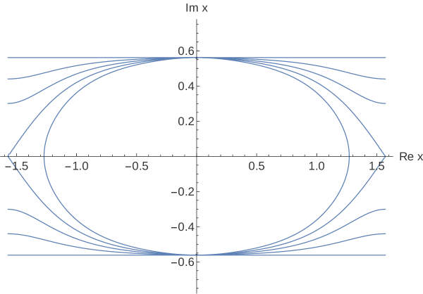
Figure 2: The curves ${\rm Re\,}\varepsilon(\lambda|h)=0$ for various values of the magnetic field. Here $\Delta=1.7$, $h_{\ell}/J=0.76$. The values of the magnetic field decrease proceeding from the inner to the outer curve: $h/h_{\ell}=1.34,1,2/3,1/3,0$. In the critical regime $h_{\ell}<h<h_{u}=4J(1+\Delta)$ the curves are closed. In this regime $\varepsilon$ is not given by (50), but is rather defined as a solution of a linear integral equation. At the lower critical field $h=h_{\ell}$ the closed curves develop two cusps, and a gap opens for $0<h<h_{\ell}$, which is the parameter regime considered in this work.

Conjecture 1.

Low-$T$ Bethe root patterns at $0<h<h_{\ell}$ [15].

1. All excitations of the quantum transfer matrix at low $T$ and large enough Trotter number $N$ can be parameterized by an even number of complex parameters located inside the strip $|{\rm Im\,}\lambda|<\gamma/2$ and by an index $\mathfrak{e}\in{\mathbb{Z}}/2{\mathbb{Z}}$. Referring to [15] we call the parameters in the upper half plane particles, the parameters in the lower half plane holes. We shall denote the set of particles by $\cal Y$, the set of holes by $\cal X$.

2. For excited states with $M_{n}=M=N+1$ we have $\operatorname{card}{\cal X}=\operatorname{card}{\cal Y}=\ell$.

3. Up to corrections of the order $T^{\infty}$ the particles and holes are determined by the low-$T$ higher-level Bethe Ansatz equations

   $$\varepsilon(y|h) =2\pi{\rm i}T\bigl{(}\ell_{y}+\mathfrak{e}/2+F(y|{\cal X},{\cal Y})\bigr{)}\,, \forall\ y\in{\cal Y}\,,$$ (55a)

   $$\varepsilon(x|h) =2\pi{\rm i}T\bigl{(}m_{x}+\mathfrak{e}/2+F(x|{\cal X},{\cal Y})\bigr{)}\,, \forall\ x\in{\cal X}\,,$$ (55b)

   where $\ell_{y},m_{x}\in{\mathbb{Z}}$ and where the $\ell_{y}$ and the $m_{x}$ are mutually distinct.

4. For solution ${\cal X}_{n}$, ${\cal Y}_{n}$ of (55) with index $\mathfrak{e}=\mathfrak{e}_{n}$ we denote $F(\lambda|{\cal X}_{n},{\cal Y}_{n})=F_{n}(\lambda)$. The auxiliary function corresponding to this solution is

   $$\mathfrak{a}_{n}(\lambda|h)=(-1)^{\mathfrak{e}_{n}}\operatorname{e}^{-\varepsilon(\lambda|h)/T+2\pi{\rm i}F_{n}(\lambda)}\bigl{(}1+{\cal O}(T^{\infty})\bigr{)}$$ (56)

   uniformly for $|{\rm Im\,}\lambda|<\gamma/2$, away from the points $\pm{\rm i}\gamma/2$.

In the limit $T\rightarrow 0+$ the higher-level Bethe Ansatz equations (55) decouple, ${\rm i}\pi\ell_{y}T$ and ${\rm i}\pi m_{x}T$ turn into independent continuous variables, and the particles and holes become free parameters on the curves

$${\cal B}_{\pm}=\bigl{\{}\lambda\in{\mathbb{C}}\big{|}{\rm Re\,}\varepsilon(\lambda|h)=0,-\pi/2\leq{\rm Re\,}\lambda\leq\pi/2,0<\pm{\rm Im\,}\lambda<\gamma\bigr{\}}\,.$$ (57)

These curves are shown in Figure 2. As we can see, the massive regime is distinguished from the massless regime by the opening of a ‘mass gap’ at the critical field $h_{\ell}$.

3.2 Low-temperature limit of the eigenvalue ratios

The main result of our work [15] was an explicit formula for all correlation lengths, or rather all eigenvalue ratios, in the low-temperature regime. At low enough temperatures all excitations are parameterized by solutions ${\cal X}_{n}$, ${\cal Y}_{n}$ of the higher-level Bethe Ansatz equations (55). Let $k=\mathfrak{e}_{n}-\mathfrak{e}_{0}$. Then, for $-\gamma<{\rm Im\,}\lambda<0$, the corresponding eigenvalue ratios in the Trotter limit and at finite magnetic field [15, 18] can be expressed as

$$\rho_{n}(\lambda|h,h^{\prime})=(-1)^{k}\exp\biggl{\{}{\rm i}\mspace{-8.0mu}\sum_{z\in{\cal X}_{n}\ominus{\cal Y}_{n}}\mspace{-16.0mu}p(\lambda-z+{\rm i}\gamma/2)\biggr{\}}\,,$$ (58)

this being valid up to multiplicative corrections of the form $\bigl{(}1+{\cal O}(T^{\infty})\bigr{)}$. Note that the value of the magnetic field $h^{\prime}$ enters here only through the particle and hole parameters.

From equation (58) we obtain the eigenvalue ratios entering the form factor series (33),

$$\rho_{n}(-{\rm i}\gamma/2|h,h^{\prime})=(-1)^{k}\exp\biggl{\{}{\rm i}\mspace{-8.0mu}\sum_{z\in{\cal Y}_{n}\ominus{\cal X}_{n}}\mspace{-16.0mu}p(z)\biggr{\}}=(-1)^{k}\mspace{-8.0mu}\prod_{z\in{\cal Y}_{n}\ominus{\cal X}_{n}}\frac{\vartheta_{1}(z-{\rm i}\gamma/2|q^{2})}{\vartheta_{4}(z-{\rm i}\gamma/2|q^{2})}\,,$$ (59)

and

$$\lim_{\begin{subarray}{c}N\rightarrow\infty\\ \varepsilon\rightarrow 0\end{subarray}}\biggl{(}\frac{\rho_{n}(-{\rm i}\gamma/2+{\rm i}t/\kappa N|h,h^{\prime})}{\rho_{n}(-{\rm i}\gamma/2-{\rm i}t/\kappa N|h,h^{\prime})}\biggr{)}^{\frac{N}{2}}=\exp\bigl{\{}({\rm i}t/\kappa)\partial_{\lambda}\ln\rho_{n}(\lambda|h,h^{\prime})\bigr{\}}_{\lambda=-{\rm i}\gamma/2}\\[4.30554pt] =\exp\biggl{\{}2{\rm i}tJ\operatorname{sh}(\gamma)\mspace{-16.0mu}\sum_{z\in{\cal X}_{n}\ominus{\cal Y}_{n}}\mspace{-16.0mu}p^{\prime}(z)\biggr{\}}=\exp\biggl{\{}{\rm i}t\mspace{-14.0mu}\sum_{z\in{\cal Y}_{n}\ominus{\cal X}_{n}}\mspace{-16.0mu}\varepsilon(z|h)\biggr{\}}\,.$$ (60)

Both formula are again valid up to multiplicative temperature corrections of the form $\bigl{(}1+{\cal O}(T^{\infty})\bigr{)}$.

3.3 Non-linear integral equations

The low-$T$ analysis can be based on a non-linear integral equation satisfied by the auxiliary functions $\mathfrak{a}_{n}(\cdot|h)$. Let us briefly recall this equation. We start with definitions and useful notation. Let

$$\theta(\lambda|\gamma)=\int_{\Gamma_{\lambda}}{\rm d}\mu\>\bigl{(}\,{\rm ctg}\,(\mu-{\rm i}\gamma)-\,{\rm ctg}\,(\mu+{\rm i}\gamma)\bigr{)}\,,$$ (61)

where $\Gamma_{\lambda}$ is a piecewise straight contour beginning at $-\frac{\pi}{2}$, running parallel to the imaginary axis to $-\frac{\pi}{2}+{\rm Im\,}\lambda$, then continuing parallel to the real axis from $-\frac{\pi}{2}+{\rm Im\,}\lambda$ to $\lambda$. This function has branch cuts along $(-\infty\pm{\rm i}\gamma,-\pi\pm{\rm i}\gamma]\cup[\pm{\rm i}\gamma,+\infty\pm{\rm i}\gamma)$ and satisfies the quasi-periodicity, quasi-reflection and asymptotic conditions

$$\theta(\lambda+\pi|\gamma) =\theta(\lambda|\gamma)+\begin{cases}2\pi{\rm i}&|{\rm Im\,}\lambda|<\gamma\\ 0&|{\rm Im\,}\lambda|>\gamma,\end{cases}$$ (62a)

$$\theta(-\lambda|\gamma) =-\theta(\lambda|\gamma)+\begin{cases}2\pi{\rm i}&|{\rm Im\,}\lambda|<\gamma\\ 0&|{\rm Im\,}\lambda|>\gamma,\end{cases}$$ (62b)

$$\lim_{{\rm Re\,}\lambda\rightarrow\pm\infty}\theta(\lambda|\gamma) =\mp 2\gamma\,.$$ (62c)

It is constructed in such a way that

$$\operatorname{e}^{\theta(\lambda|\gamma)}=\frac{\sin(\lambda-{\rm i}\gamma)}{\sin(\lambda+{\rm i}\gamma)}\,.$$ (63)

For $\gamma>0$ we also set

$$K_{0}(\lambda|\gamma)=\frac{\theta^{\prime}(\lambda|\gamma)}{2\pi{\rm i}}\,.$$ (64)

Then $K_{0}(\lambda|\gamma)>0$ for $\lambda\in{\mathbb{R}}$. Now define

$$\varepsilon^{(N,\varepsilon)}_{0}(\lambda|h)=h+T\bigl{\{}\theta\bigl{(}\lambda-\varepsilon\big{|}{\textstyle\frac{\gamma}{2}}\bigr{)}-\theta\bigl{(}\lambda+\varepsilon\big{|}{\textstyle\frac{\gamma}{2}}\bigr{)}\bigr{\}}$$ (65)

$$\mspace{0.9mu}+\frac{NT}{2}\Bigl{\{}\theta\bigl{(}\lambda+{\textstyle\frac{{\rm i}t}{\kappa N}}\big{|}{\textstyle\frac{\gamma}{2}}\bigr{)}-\theta\bigl{(}\lambda-{\textstyle\frac{{\rm i}t}{\kappa N}}\big{|}{\textstyle\frac{\gamma}{2}}\bigr{)}+\theta\bigl{(}\lambda-{\textstyle\frac{{\rm i}t+1/T}{\kappa N}}\big{|}{\textstyle\frac{\gamma}{2}}\bigr{)}-\theta\bigl{(}\lambda+{\textstyle\frac{{\rm i}t+1/T}{\kappa N}}\big{|}{\textstyle\frac{\gamma}{2}}\bigr{)}\Bigr{\}}\,.$$

This function has the point-wise limit

$$\lim_{N\rightarrow\infty}\lim_{\varepsilon\rightarrow 0}\varepsilon^{(N,\varepsilon)}_{0}(\lambda|h)=h-\theta^{\prime}\bigl{(}\lambda|{\textstyle\frac{\gamma}{2}}\bigr{)}/\kappa=h-4\pi J\operatorname{sh}(\gamma)K_{0}\bigl{(}\lambda|{\textstyle\frac{\gamma}{2}}\bigr{)}=\varepsilon_{0}(\lambda|h)$$ (66)

which is independent of $t$ and $T$.

For a shortcut in the derivation of the non-linear integral equation we shall now use our insight from previous work [15] summarized above as an input. Recall that we have fixed a solution $\{\mu_{j}\}_{j=1}^{M}=\{\lambda_{j}^{(n)}\}_{j=1}^{M_{n}}$ of the Bethe ansatz equations (19) which determines an auxiliary function $\mathfrak{a}_{n}(\cdot|h^{\prime})$ and that we are keeping the magnetic field $h$ pertaining to the dominant state and $h^{\prime}$ pertaining to the $n$th excited state independent. Let us now assume that for fixed small $T$ and $N$ large enough all Bethe roots $\mu_{j}$ are close to ${\cal B}_{\pm}$, such that $|{\rm Im\,}\mu_{j}|<\gamma/2$, $j=1,\dots,M$. Using (63) and (65) in (18) we see that

$$\ln\mathfrak{a}_{n}(\lambda|h^{\prime})=-\frac{\varepsilon_{0}^{(N,\varepsilon)}(\lambda|h^{\prime})}{T}+\sum_{j=1}^{N+1}\theta(\lambda-\mu_{j}|\gamma)\\ -\frac{N}{2}\Bigl{\{}\theta\bigl{(}\lambda+{\textstyle\frac{{\rm i}\gamma}{2}}-{\textstyle\frac{{\rm i}t}{\kappa N}}\big{|}\gamma\bigr{)}+\theta\bigl{(}\lambda+{\textstyle\frac{{\rm i}\gamma}{2}}+{\textstyle\frac{{\rm i}t+1/T}{\kappa N}}\big{|}\gamma\bigr{)}\Bigr{\}}-\theta\bigl{(}\lambda+{\textstyle\frac{{\rm i}\gamma}{2}}+\varepsilon\big{|}\gamma\bigr{)}$$ (67)

is a possible definition of the logarithm of $\mathfrak{a}_{n}(\cdot|h^{\prime})$. This definition guarantees that $\ln\mathfrak{a}_{n}(\cdot|h^{\prime})$ is $\pi$-periodic and analytic for $|{\rm Im\,}\lambda|<\gamma/2$ in the following sense. For a given $\lambda$ with $|{\rm Im\,}\lambda|<\gamma/2$ and small $T>0$ there is an $N_{0}\in{\mathbb{N}}$ such that $\ln\mathfrak{a}_{n}(\cdot|h^{\prime})$ is analytic in $\lambda$ and

$$\ln\mathfrak{a}_{n}(\lambda+\pi|h^{\prime})=\ln\mathfrak{a}_{n}(\lambda|h^{\prime})$$ (68)

for all $N>N_{0}$.

We fix a simple closed and positively oriented contour ${\cal C}={\cal C}_{l}+{\cal C}_{-}+{\cal C}_{r}+{\cal C}_{+}$, where

$${\cal C}_{l} =[-\pi/2,-\pi/2-{\rm i}\gamma/2-{\rm i}0]\,, {\cal C}_{r} =-{\cal C}_{l}+\pi\,,$$ (69)

$${\cal C}_{+} =[\pi/2,-\pi/2]\,, {\cal C}_{-} =-{\cal C}_{+}-{\rm i}\gamma/2-{\rm i}0\,.$$ (70)

Here the regularization ${\rm i}0$ means that the pole of $\mathfrak{a}_{n}(\lambda|h^{\prime})$ at $\lambda=-\frac{{\rm i}\gamma}{2}+\frac{{\rm i}t}{\kappa N}$ is inside ${\cal C}$.

Let

$${\cal Z}_{n}=\{\lambda\in{\mathbb{C}}|1+\mathfrak{a}_{n}(\lambda|h^{\prime})=0\}\cap\operatorname{Int}{\cal C}\,.$$ (71)

With $\{\mu_{j}\}_{j=1}^{M}$ we associate sets of ‘particles’ ${\cal Y}_{n}$ and ‘holes’ ${\cal X}_{n}$ relative to ${\cal C}$, setting

$${\cal Y}_{n}=\{\mu_{j}\}_{j=1}^{M}\cap\operatorname{Ext}{\cal C}\,,\quad{\cal X}_{n}={\cal Z}_{n}\setminus\bigl{(}\{\mu_{j}\}_{j=1}^{M}\cap\operatorname{Int}{\cal C}\bigr{)}\,.$$ (72)

Using the residue theorem in (67) then implies that

$$\ln\mathfrak{a}_{n}(\lambda|h^{\prime})=-\frac{\varepsilon_{0}^{(N,\varepsilon)}(\lambda|h^{\prime})}{T}+\mspace{-18.0mu}\sum_{z\in{\cal Y}_{n}\ominus{\cal X}_{n}}\mspace{-18.0mu}\theta(\lambda-z|\gamma)+\int_{\cal C}\frac{{\rm d}\mu}{2\pi{\rm i}}\theta(\lambda-\mu|\gamma)\frac{\partial_{\mu}\mathfrak{a}_{n}(\mu|h^{\prime})}{1+\mathfrak{a}_{n}(\mu|h^{\prime})}$$ (73)

for all $\lambda\in{\mathbb{C}}$ with $|{\rm Im\,}\lambda|<\gamma/2$. Here we have used that, due to our assumptions, $\mu_{j}-{\rm i}\gamma\notin\operatorname{Int}{\cal C}$.

Equation (73) turns into a non-linear integral equation for $\mathfrak{a}_{n}(\cdot|h^{\prime})$ upon applying partial integration to the integral. For this purpose a proper definition of the logarithm of $1+\mathfrak{a}_{n}(\cdot|h^{\prime})$ is required. Let us assume (56) to hold approximately for small $T$ and $N$ large enough. Then $|\mathfrak{a}_{n}(\lambda|h^{\prime})|=1$, $-\gamma/2<{\rm Im\,}\lambda<0$ determines a curve ${\cal B}_{n}$ close to ${\cal B}_{-}$ which intersects the line ${\rm Re\,}\lambda=-\frac{\pi}{2}$ in a point $-\frac{\pi}{2}-{\rm i}x_{0}$ with $-\gamma/2<x_{0}<0$. Due to the $\pi$-periodicity of $\mathfrak{a}_{n}(\cdot|h^{\prime})$ the curve ${\cal B}_{n}$ passes through $\frac{\pi}{2}-{\rm i}x_{0}$ as well. Define a domain ${\cal D}_{\uparrow}$ located between ${\cal B}_{n}$ and the real axis and a domain ${\cal D}_{\downarrow}$ located between the line ${\rm Im\,}\lambda=-\frac{\gamma}{2}$ and ${\cal B}_{n}$. Then

$$|\mathfrak{a}_{n}(\lambda|h^{\prime})|\begin{cases}>1&\text{for $\lambda\in{\cal D}_{\uparrow}$}\\ <1&\text{for $\lambda\in{\cal D}_{\downarrow}$.}\end{cases}$$ (74)

This allows us to define the logarithm of $1+\mathfrak{a}_{n}(\cdot|h^{\prime})$ on ${\cal D}_{\uparrow}\cup{\cal D}_{\downarrow}$ as an analytic and $\pi$-periodic function,

$$\operatorname{Ln}(1+\mathfrak{a}_{n})(\lambda|h^{\prime})=\begin{cases}\ln\mathfrak{a}_{n}(\lambda|h^{\prime})+\ln\bigl{(}1+1/\mathfrak{a}_{n}(\lambda|h^{\prime})\bigr{)}&\text{for $\lambda\in{\cal D}_{\uparrow}$}\\[2.15277pt] \ln\bigl{(}1+\mathfrak{a}_{n}(\lambda|h^{\prime})\bigr{)}&\text{for $\lambda\in{\cal D}_{\downarrow}$,}\end{cases}$$ (75)

where $\ln\mathfrak{a}_{n}(\cdot|h^{\prime})$ is defined by (67) and the other logarithms on the right hand side are defined by the principal branch. By construction $\operatorname{Ln}(1+\mathfrak{a}_{n})(\cdot|h^{\prime})$ has jump discontinuities across ${\cal B}_{n}$. In particular, at $\mp\frac{\pi}{2}-{\rm i}x_{0}$

$$\operatorname{Ln}(1+\mathfrak{a}_{n})\bigl{(}\mp{\textstyle\frac{\pi}{2}}-{\rm i}x_{0}^{-}\big{|}h^{\prime}\bigr{)}-\operatorname{Ln}(1+\mathfrak{a}_{n})\bigl{(}\mp{\textstyle\frac{\pi}{2}}-{\rm i}x_{0}^{+}\big{|}h^{\prime}\bigr{)}=2\pi{\rm i}\mathfrak{e}_{n}$$ (76)

for some $\mathfrak{e}_{n}\in{\mathbb{Z}}$.

Using the properties of the function $\operatorname{Ln}(1+\mathfrak{a}_{n})(\cdot|h^{\prime})$ we may now calculate the index of $1+\mathfrak{a}_{n}(\cdot|h^{\prime})$ along ${\cal C}$,

$$\int_{\cal C}\frac{{\rm d}\mu}{2\pi{\rm i}}\frac{\partial_{\mu}\mathfrak{a}_{n}(\mu|h^{\prime})}{1+\mathfrak{a}_{n}(\mu|h^{\prime})}=\operatorname{Ln}(1+\mathfrak{a}_{n})\bigl{(}-{\textstyle\frac{\pi}{2}}-{\rm i}x_{0}^{-}\big{|}h^{\prime}\bigr{)}-\operatorname{Ln}(1+\mathfrak{a}_{n})\bigl{(}{\textstyle\frac{\pi}{2}}-{\rm i}x_{0}^{-}\big{|}h^{\prime}\bigr{)}\\ +\operatorname{Ln}(1+\mathfrak{a}_{n})\bigl{(}{\textstyle\frac{\pi}{2}}-{\rm i}x_{0}^{+}\big{|}h^{\prime}\bigr{)}-\operatorname{Ln}(1+\mathfrak{a}_{n})\bigl{(}-{\textstyle\frac{\pi}{2}}-{\rm i}x_{0}^{+}\big{|}h^{\prime}\bigr{)}=0\,.$$ (77)

Here we have used the analyticity of $\operatorname{Ln}(1+\mathfrak{a}_{n})(\cdot|h^{\prime})$ in ${\cal D}_{\uparrow}$ und ${\cal D}_{\downarrow}$ in the first equation and (76) in the second equation. Calculating the same integral by means of the residue theorem we see that

$$\int_{\cal C}\frac{{\rm d}\mu}{2\pi{\rm i}}\frac{\partial_{\mu}\mathfrak{a}_{n}(\mu|h^{\prime})}{1+\mathfrak{a}_{n}(\mu|h^{\prime})}=\operatorname{card}{\cal Y}_{n}-\operatorname{card}{\cal X}_{n}\,,$$ (78)

implying that

$$\operatorname{card}{\cal Y}_{n}=\operatorname{card}{\cal X}_{n}=\ell\,.$$ (79)

Performing a similar calculation as in (77) and using also the quasi-periodicity (62) of the function $\theta(\cdot|\gamma)$ we may now rewrite the integral on the right hand side of (73),

$$\int_{\cal C}\frac{{\rm d}\mu}{2\pi{\rm i}}\theta(\lambda-\mu|\gamma)\frac{\partial_{\mu}\mathfrak{a}_{n}(\mu|h^{\prime})}{1+\mathfrak{a}_{n}(\mu|h^{\prime})}=2\pi{\rm i}\mathfrak{e}_{n}+\int_{\cal C}{\rm d}\mu\>K_{0}(\lambda-\mu|\gamma)\operatorname{Ln}(1+\mathfrak{a}_{n})(\mu|h^{\prime})\,.$$ (80)

Inserting this back into (73) we have converted the latter equation into a non-linear integral equation for the function $\mathfrak{a}_{n}(\cdot|h^{\prime})$,

$$\ln\mathfrak{a}_{n}(\lambda|h^{\prime})=-\frac{\varepsilon_{0}^{(N,\varepsilon)}(\lambda|h^{\prime})}{T}\\ +2\pi{\rm i}\mathfrak{e}_{n}+\mspace{-18.0mu}\sum_{z\in{\cal Y}_{n}\ominus{\cal X}_{n}}\mspace{-18.0mu}\theta(\lambda-z|\gamma)+\int_{\cal C}{\rm d}\mu\>K_{0}(\lambda-\mu|\gamma)\operatorname{Ln}(1+\mathfrak{a}_{n})(\mu|h^{\prime})\,.$$ (81)

This equation determines $\mathfrak{a}_{n}(\cdot|h^{\prime})$ on ${\cal C}$ and then, by analytic continuation in the entire complex plane. Recall that, $\mathfrak{a}_{n}(x|h^{\prime})=\mathfrak{a}_{n}(y|h^{\prime})=-1$ for all $x\in{\cal X}_{n}$, $y\in{\cal Y}_{n}$ by construction.

Remark 1.

The non-linear integral equation (81) is appropriate for taking the Trotter limit of the function $\mathfrak{a}_{n}(\cdot|h^{\prime})$. Formally we just have to replace the function $\varepsilon_{0}^{(N,\varepsilon)}(\cdot|h^{\prime})$ by its limit $\varepsilon_{0}(\cdot|h^{\prime})$ defined in (66).

Remark 2.

Reversing the steps in the derivation of (77) and (81) we can go back to the Bethe Ansatz equations (19). This means that every solution of the non-linear integral equation for which $1+\mathfrak{a}_{n}(\cdot|h^{\prime})$ has index zero corresponds to a solution of the Bethe Ansatz equation and to an eigenstate of the dynamical quantum transfer matrix. In [15] we argued that, in the low-$T$ limit, all eigenstates can be obtained this way.

We shall also need an ‘off-shell version’ of the auxiliary function $\mathfrak{a}_{n}(\cdot|h^{\prime})$ which is defined by means of a non-linear integral equation similar to (81). In order to construct it we first of all set

$$\overline{\varepsilon}_{0}^{(N,\varepsilon)}(\lambda|h)=h+T\bigl{\{}\theta\bigl{(}\lambda+{\rm i}\gamma+\varepsilon\big{|}{\textstyle\frac{\gamma}{2}}\bigr{)}-\theta\bigl{(}\lambda+{\rm i}\gamma-\varepsilon\big{|}{\textstyle\frac{\gamma}{2}}\bigr{)}\bigr{\}}$$

$$\mspace{72.0mu}+\frac{NT}{2}\Bigl{\{}\theta\bigl{(}\lambda+{\rm i}\gamma-{\textstyle\frac{{\rm i}t}{\kappa N}}\big{|}{\textstyle\frac{\gamma}{2}}\bigr{)}-\theta\bigl{(}\lambda+{\rm i}\gamma+{\textstyle\frac{{\rm i}t}{\kappa N}}\big{|}{\textstyle\frac{\gamma}{2}}\bigr{)}$$

$$\mspace{162.0mu}+\theta\bigl{(}\lambda+{\rm i}\gamma+{\textstyle\frac{{\rm i}t+1/T}{\kappa N}}\big{|}{\textstyle\frac{\gamma}{2}}\bigr{)}-\theta\bigl{(}\lambda+{\rm i}\gamma-{\textstyle\frac{{\rm i}t+1/T}{\kappa N}}\big{|}{\textstyle\frac{\gamma}{2}}\bigr{)}\Bigr{\}}$$ (82)

Then, for every pair of sets ${\cal U}\subset\operatorname{Int}{\cal C}$, ${\cal V}\subset\operatorname{Ext}{\cal C}$ with $\operatorname{card}{\cal U}=\operatorname{card}{\cal V}=\ell$, the function $\mathfrak{a}^{-}(\cdot|{\cal U},{\cal V},h^{\prime})$ is the solution of the non-linear integral equation

$$\ln\mathfrak{a}^{-}(\lambda|{\cal U},{\cal V},h^{\prime})=\frac{\overline{\varepsilon}_{0}^{(N,\varepsilon)}(\lambda|h^{\prime})}{T}\\ -2\pi{\rm i}\mathfrak{e}_{n}^{\prime}-\mspace{-12.0mu}\sum_{z\in{\cal V}\ominus{\cal U}}\mspace{-8.0mu}\theta(\lambda-z|\gamma)-\int_{\cal C}{\rm d}\mu\>K_{0}(\lambda-\mu|\gamma)\operatorname{Ln}^{-}(1+\mathfrak{a}^{-})(\mu|{\cal U},{\cal V},h^{\prime})\,.$$ (83)

Here

$$\operatorname{Ln}^{-}(1+\mathfrak{a}^{-})(\lambda|{\cal U},{\cal V},h^{\prime})\\ =\begin{cases}\ln\bigl{(}1+\mathfrak{a}^{-}(\lambda|{\cal U},{\cal V},h^{\prime})\bigr{)}&\text{for $\lambda\in{\cal D}_{\uparrow}^{-}$}\\[2.15277pt] \ln\mathfrak{a}^{-}(\lambda|{\cal U},{\cal V},h^{\prime})\bigr{)}+\ln\bigl{(}1+1/\mathfrak{a}^{-}(\lambda|{\cal U},{\cal V},h^{\prime})\bigr{)}&\text{for $\lambda\in{\cal D}_{\downarrow}^{-}$,}\end{cases}$$ (84)

and ${\cal D}_{\uparrow}^{-}$ and ${\cal D}_{\downarrow}^{-}$ are separated by the line, where $|\mathfrak{a}^{-}(\lambda|{\cal U},{\cal V},h^{\prime})\bigr{)}|=1$. The contour ${\cal C}$ is the same as in (81) but properly regularized such as to include the point $-\frac{{\rm i}\gamma}{2}+\frac{{\rm i}t+1/T}{\kappa N}$ for sufficiently large values of $N$. The integral equation (83) is constructed in such a way that

$$\mathfrak{a}_{n}(\cdot|h^{\prime})=1/\mathfrak{a}^{-}(\cdot|{\cal X}_{n},{\cal Y}_{n},h^{\prime})$$ (85)

if ${\cal X}_{n}$ and ${\cal Y}_{n}$ are solutions of the subsidiary conditions $\mathfrak{a}^{-}(x|{\cal X}_{n},{\cal Y}_{n},h^{\prime})=-1$ for all $x\in{\cal X}_{n}$, and $\mathfrak{a}^{-}(y|{\cal X}_{n},{\cal Y}_{n},h^{\prime})=-1$ for all $y\in{\cal Y}_{n}$.

Hence, it is natural to define an off-shell function

$$\mathfrak{a}^{+}(\cdot|{\cal U},{\cal V},h^{\prime})=1/\mathfrak{a}^{-}(\cdot|{\cal U},{\cal V},h^{\prime})\,.$$ (86)

Then

$$\mathfrak{a}_{n}(\cdot|h^{\prime}) =\mathfrak{a}^{+}(\cdot|{\cal X}_{n},{\cal Y}_{n},h^{\prime})=\mathfrak{a}_{n}^{+}(\cdot|h^{\prime})\,,$$ (87a)

$$1/\mathfrak{a}_{n}(\cdot|h^{\prime}) =\mathfrak{a}^{-}(\cdot|{\cal X}_{n},{\cal Y}_{n},h^{\prime})=\mathfrak{a}_{n}^{-}(\cdot|h^{\prime})\,.$$ (87b)

4 Low-temperature analysis of the amplitudes

In this section we derive explicit expressions for the amplitudes (31) in the low-temperature limit.

4.1 A factorization of determinants

Denoting the elements of ${\cal X}_{n}$ by $x_{j}$, the elements of ${\cal Y}_{n}$ by $y_{j}$ and the elements of ${\cal Z}_{n}$ by $z_{j}$ (cf. (71), (72)) we may label them in such a way that

$$z_{j} =\mu_{j}\,, j=1,\dots,M-\ell\,,$$

$$y_{j} =\mu_{M-\ell+j}\,, j=1,\dots,\ell\,,$$

$$x_{j} =z_{M-\ell+j}\,, j=1,\dots,\ell\,.$$ (88)

Using this notation we shall separate the particle- hole contributions from the determinants on the right hand side of (37). We first define a number of auxiliary matrices through their matrix elements. For these we shall use a convention in which upper indices refer to rows and lower indices to columns. Let

$$K^{j}_{k} =\frac{K(\lambda_{j}-\lambda_{k})}{\mathfrak{a}^{\prime}(\lambda_{k}|h)}\,, j,k=1,\dots,M\,,$$

$$V^{j}_{k} =\frac{\operatorname{e}(\lambda_{j}-\mu_{k})}{1+\mathfrak{a}(\mu_{k}|h)}-\frac{\operatorname{e}(\mu_{k}-\lambda_{j})}{1+1/\mathfrak{a}(\mu_{k}|h)}\,, j,k=1,\dots,M\,.$$ (89)

Further define

$${V^{(i)}}^{j}_{k} =V^{j}_{k}\,, j=1,\dots,M;k=1,\dots,M-\ell\,,$$

$${V^{(p)}}^{j}_{k} =V^{j}_{M-\ell+k}\,, j=1,\dots,M;k=1,\dots,\ell\,,$$

$${V^{(h)}}^{j}_{k} =\frac{\operatorname{e}(\lambda_{j}-x_{k})}{1+\mathfrak{a}(x_{k}|h)}-\frac{\operatorname{e}(x_{k}-\lambda_{j})}{1+1/\mathfrak{a}(x_{k}|h)}\,, j=1,\dots,M;k=1,\dots,\ell$$ (90)

and

$$G=(I_{M}+K)^{-1}\bigl{(}V^{(i)},V^{(h)}\bigr{)}\,,\quad D=(0,I_{\ell})G^{-1}(I_{M}+K)^{-1}V^{(p)}\,.$$ (91)

Here and in the following $I_{n}$ denotes the $n\times n$ unit matrix, and we use a block-matrix notation. E.g., in $\bigl{(}V^{(i)},V^{(h)}\bigr{)}$ we combine the $M\times(M-\ell)$ block $V^{(i)}$ and the $M\times\ell$ block $V^{(h)}$ into an $M\times M$ square matrix. Similarly, $(0,I_{\ell})$ consists of an $\ell\times(M-\ell)$ block of zeros, combined with the $\ell\times\ell$ unit matrix into an $\ell\times M$ matrix. This convention is particularly convenient for the proofs of the two following lemmata.

Lemma 2.

A factorization of determinants.
We have the following factorization of determinants,

$$\frac{\det_{M}\Bigl{\{}\frac{\operatorname{e}(\lambda_{j}-\mu_{k})}{1+\mathfrak{a}(\mu_{k}|h)}-\frac{\operatorname{e}(\mu_{k}-\lambda_{j})}{1+1/\mathfrak{a}(\mu_{k}|h)}\Bigr{\}}}{\det_{M}\Bigl{\{}\delta^{j}_{k}+\frac{K(\lambda_{j}-\lambda_{k})}{\mathfrak{a}^{\prime}(\lambda_{k}|h)}\Bigr{\}}}=\det_{M}\{G\}\det_{\ell}\{D\}\,.$$ (92)

Proof.

With the notations above we can write

$$\frac{\det_{M}\Bigl{\{}\frac{\operatorname{e}(\lambda_{j}-\mu_{k})}{1+\mathfrak{a}(\mu_{k}|h)}-\frac{\operatorname{e}(\mu_{k}-\lambda_{j})}{1+1/\mathfrak{a}(\mu_{k}|h)}\Bigr{\}}}{\det_{M}\Bigl{\{}\delta^{j}_{k}+\frac{K(\lambda_{j}-\lambda_{k})}{\mathfrak{a}^{\prime}(\lambda_{k}|h)}\Bigr{\}}}=\det_{M}\bigl{(}(I_{M}+K)^{-1}\bigr{)}\det_{M}\bigl{(}(V^{(i)},V^{(p)})\bigr{)}\,.$$ (93)

Now

$$\det_{M}\bigl{(}(V^{(i)},V^{(p)})\bigr{)}=\det_{M+\ell}\begin{bmatrix}V^{(i)}&V^{(p)}&V^{(h)}\\ 0&0&I_{\ell}\end{bmatrix}=\det_{M+\ell}\begin{bmatrix}V^{(i)}&V^{(h)}&V^{(p)}\\ 0&-I_{\ell}&0\end{bmatrix}.$$ (94)

Hence,

$$\det_{M}\bigl{(}(I_{M}+K)^{-1}\bigr{)}\det_{M}\bigl{(}(V^{(i)},V^{(p)})\bigr{)}=\det_{M+\ell}\begin{bmatrix}G&(I_{M}+K)^{-1}V^{(p)}\\ (0,-I_{\ell})&0\end{bmatrix}\\[4.30554pt] =\det_{M}\{G\}\det_{M+\ell}\begin{bmatrix}I_{M}&G^{-1}(I_{M}+K)^{-1}V^{(p)}\\ (0,-I_{\ell})&0\end{bmatrix}\\[4.30554pt] =\det_{M}\{G\}\det_{M+\ell}\begin{bmatrix}I_{M}&G^{-1}(I_{M}+K)^{-1}V^{(p)}\\ 0&(0,I_{\ell})G^{-1}(I_{M}+K)^{-1}V^{(p)}\end{bmatrix}$$ (95)

which implies (92). ∎

In order to perform a similar calculation with the second such ratio on the right hand side of (37) we have to decompose the norm determinant in the denominator first. For this purpose let

$$L^{j}_{k} =\frac{K(\mu_{j}-\mu_{k})}{\mathfrak{a}_{n}^{\prime}(\mu_{k}|h^{\prime})}\,, j,k=1,\dots,M\,,$$

$${L^{(ii)}}^{j}_{k} =\frac{K(\mu_{j}-\mu_{k})}{\mathfrak{a}_{n}^{\prime}(\mu_{k}|h^{\prime})}\,, j,k=1,\dots,M-\ell\,,$$

$${L^{(ip)}}^{j}_{k} =\frac{K(\mu_{j}-y_{k})}{\mathfrak{a}_{n}^{\prime}(y_{k}|h^{\prime})}\,, j=1,\dots,M-\ell;k=1,\dots,\ell\,,$$

$${L^{(pi)}}^{j}_{k} =\frac{K(y_{j}-\mu_{k})}{\mathfrak{a}_{n}^{\prime}(\mu_{k}|h^{\prime})}\,, j=1,\dots,\ell;k=1,\dots,M-\ell\,,$$

$${L^{(pp)}}^{j}_{k} =\frac{K(y_{j}-y_{k})}{\mathfrak{a}_{n}^{\prime}(y_{k}|h^{\prime})}\,, j,k=1,\dots,\ell\,,$$

$${L^{(ih)}}^{j}_{k} =\frac{K(\mu_{j}-x_{k})}{\mathfrak{a}_{n}^{\prime}(x_{k}|h^{\prime})}\,, j=1,\dots,M-\ell;k=1,\dots,\ell\,,$$

$${L^{(hi)}}^{j}_{k} =\frac{K(x_{j}-\mu_{k})}{\mathfrak{a}_{n}^{\prime}(\mu_{k}|h^{\prime})}\,, j=1,\dots,\ell;k=1,\dots,M-\ell\,,$$

$${L^{(hh)}}^{j}_{k} =\frac{K(x_{j}-x_{k})}{\mathfrak{a}_{n}^{\prime}(x_{k}|h^{\prime})}\,, j,k=1,\dots,\ell\,,$$

$${L^{(ph)}}^{j}_{k} =\frac{K(y_{j}-x_{k})}{\mathfrak{a}_{n}^{\prime}(x_{k}|h^{\prime})}\,, j,k=1,\dots,\ell\,,$$

$${L^{(hp)}}^{j}_{k} =\frac{K(x_{j}-y_{k})}{\mathfrak{a}_{n}^{\prime}(y_{k}|h^{\prime})}\,, j,k=1,\dots,\ell$$ (96)

and

$$K^{*}=\begin{pmatrix}L^{(ii)}&L^{(ih)}\\ L^{(hi)}&L^{(hh)}\end{pmatrix},$$

$$C=\begin{pmatrix}L^{(hi)}&L^{(hh)}\\ L^{(pi)}&L^{(ph)}\end{pmatrix},\ B=\begin{pmatrix}L^{(ih)}&-L^{(ip)}\\ L^{(hh)}&-L^{(hp)}\end{pmatrix},\ D=I_{2\ell}+\begin{pmatrix}-L^{(hh)}&L^{(hp)}\\ -L^{(ph)}&L^{(pp)}\end{pmatrix},$$

$$J=D+C(I_{M}+K^{*})^{-1}B\,.$$ (97)

Finally define

$${W^{(i)}}^{j}_{k} =\frac{\operatorname{e}(\mu_{j}-\lambda_{k})}{1+\mathfrak{a}_{n}(\lambda_{k}|h^{\prime})}-\frac{\operatorname{e}(\lambda_{k}-\mu_{j})}{1+1/\mathfrak{a}_{n}(\lambda_{k}|h^{\prime})}\,, j=1,\dots,M-\ell;k=1,\dots,M\,,$$

$${W^{(p)}}^{j}_{k} =\frac{\operatorname{e}(y_{j}-\lambda_{k})}{1+\mathfrak{a}_{n}(\lambda_{k}|h^{\prime})}-\frac{\operatorname{e}(\lambda_{k}-y_{j})}{1+1/\mathfrak{a}_{n}(\lambda_{k}|h^{\prime})}\,, j=1,\dots,\ell;k=1,\dots,M\,,$$

$${W^{(h)}}^{j}_{k} =\frac{\operatorname{e}(x_{j}-\lambda_{k})}{1+\mathfrak{a}_{n}(\lambda_{k}|h^{\prime})}-\frac{\operatorname{e}(\lambda_{k}-x_{j})}{1+1/\mathfrak{a}_{n}(\lambda_{k}|h^{\prime})}\,, j=1,\dots,\ell;k=1,\dots,M$$ (98)

and

$$G^{*}=(I_{M}+K^{*})^{-1}\begin{pmatrix}W^{(i)}\\ W^{(h)}\end{pmatrix}\,,\quad D^{*}=W^{(p)}{G^{*}}^{-1}(I_{M}+K^{*})^{-1}\binom{0}{I_{\ell}}\,.$$ (99)

With this notation we can state our next lemma.

Lemma 3.

Another factorization of determinants.
The remaining determinants in (37) admit the factorization

$$\det_{M}\biggl{\{}\delta^{j}_{k}+\frac{K(\mu_{j}-\mu_{k})}{\mathfrak{a}_{n}^{\prime}(\mu_{k}|h^{\prime})}\biggr{\}}=\det_{M}\{I_{M}+K^{*}\}\det_{2\ell}\{J\}\,,$$ (100a)

$$\frac{\det_{M}\Bigl{\{}\frac{\operatorname{e}(\mu_{j}-\lambda_{k})}{1+\mathfrak{a}_{n}(\lambda_{k}|h^{\prime})}-\frac{\operatorname{e}(\lambda_{k}-\mu_{j})}{1+1/\mathfrak{a}_{n}(\lambda_{k}|h^{\prime})}\Bigr{\}}}{\det_{M}\{I_{M}+K^{*}\}}=\det_{M}\{G^{*}\}\det_{\ell}\{D^{*}\}\,.$$ (100b)

Proof.

The proof is similar to the proof of Lemma 2 and relies on elementary row- and column manipulations of determinants. ∎

In lemma 2 and 3 we have factorized the determinants in the original representation (37) of the form factor amplitudes for the generating function in a way that will allow us to take the Trotter limit and the zero temperature limit. Two of the determinants are of size $M$, which goes to infinity for $N\rightarrow\infty$. We shall call them the ‘large determinants’. The three remaining determinants are of size $\ell$, or $2\ell$ and will be called the ‘small determinants’. In the following subsections the five determinants will be considered one by one. We shall see that the matrix elements of $G$, $G^{*}$, $(I_{M}+K)^{-1}$ and $(I_{M}+K^{*})^{-1}$ can be expressed in terms of functions that solve linear integral equations and can be explicitly calculated in the limit $T\rightarrow 0+$.

4.2 The small determinant in the denominator

We start with the $2\ell\times 2\ell$ determinant in (100a) whose structure is familiar to us from previous work [18, 22]. We first of all observe that

$$J=I_{2\ell}\\[4.30554pt] +\begin{pmatrix}-L^{(hh)}+L^{(hv)}(I_{M}+K^{*})^{-1}L^{(vh)}&L^{(hp)}-L^{(hv)}(I_{M}+K^{*})^{-1}L^{(vp)}\\ -L^{(ph)}+L^{(pv)}(I_{M}+K^{*})^{-1}L^{(vh)}&L^{(pp)}-L^{(pv)}(I_{M}+K^{*})^{-1}L^{(vp)}\end{pmatrix}\,,$$ (101)

where

$$L^{(hv)} =\bigl{(}L^{(hi)},L^{(hh)}\bigr{)}\,, L^{(pv)}=\bigl{(}L^{(pi)},L^{(ph)}\bigr{)}\,,$$ (102a)

$$L^{(vh)} =\binom{L^{(ih)}}{L^{(hh)}}\,, L^{(vp)}=\binom{L^{(ip)}}{L^{(hp)}}\,.$$ (102b)

In order to simplify (101) we define a resolvent kernel as the solution of the linear integral equation

$$R^{*}(\lambda,\mu)=K(\lambda-\mu)-\int_{\cal C}\frac{{\rm d}\nu}{2\pi{\rm i}}\frac{K(\lambda-\nu)R^{*}(\nu,\mu)}{1+\mathfrak{a}_{n}(\nu|h^{\prime})}\,.$$ (103)

Recall that $R^{*}(\lambda,\mu)$ then also satisfies the integral equation

$$R^{*}(\lambda,\mu)=K(\lambda-\mu)-\int_{\cal C}\frac{{\rm d}\nu}{2\pi{\rm i}}\frac{R^{*}(\lambda,\nu)K(\nu-\mu)}{1+\mathfrak{a}_{n}(\nu|h^{\prime})}\,.$$ (104)

Let $\lambda\in\operatorname{Int}{\cal C}$. The contour ${\cal C}$ is constructed in such a way that $\mu\in\operatorname{Int}{\cal C}\cup{\cal Y}_{n}$ implies that $\mu\pm{\rm i}\gamma\in\operatorname{Ext}{\cal C}$. Hence, $R^{*}(\cdot,\mu)$ is holomorphic in $\operatorname{Int}{\cal C}$ and on the boundary of this domain. Then the residue theorem applied to (103) implies that

$$R^{*}(\lambda,\mu)=K(\lambda-\mu)-\sum_{l=1}^{M}\frac{K(\lambda-z_{l})R^{*}(z_{l},\mu)}{\mathfrak{a}_{n}^{\prime}(z_{l}|h^{\prime})}$$ (105)

for all $\mu\in{\cal Z}_{n}\cup{\cal Y}_{n}$ and for all $\lambda\in\operatorname{Int}{\cal C}$. Equation (105) also defines the analytic continuation of $R^{*}(\cdot,\mu)$ to the complex plane. Similarly, (104) implies that

$$R^{*}(\lambda,\mu)=K(\lambda-\mu)-\sum_{l=1}^{M}\frac{R^{*}(\lambda,z_{l})K(z_{l}-\mu)}{\mathfrak{a}_{n}^{\prime}(z_{l}|h^{\prime})}$$ (106)

for all $\lambda\in{\cal Z}_{n}\cup{\cal Y}_{n}$, for all $\mu\in\operatorname{Int}{\cal C}$, and also for $\mu\in{\mathbb{C}}$ for which the right hand side is defined by analytic continuation.

Upon defining a matrix $R^{*}$ with matrix elements

$${R^{*}}^{j}_{k}=\frac{R^{*}(z_{j},z_{k})}{\mathfrak{a}_{n}^{\prime}(z_{k}|h^{\prime})}$$ (107)

equation (105) implies that

$$(I_{M}+K^{*})^{-1}=I_{M}-R^{*}\,.$$ (108)

This can be used to derive the following

Lemma 4.

Jacobian of higher level Bethe Ansatz equations [22].
The small determinant $\det_{2\ell}\{J\}$ has the representations

$$\det_{2\ell}\{J\}=\det_{2\ell}\begin{pmatrix}\delta^{j}_{k}-\frac{R^{*}(x_{j},x_{k})}{\mathfrak{a}_{n}^{\prime}(x_{k}|h^{\prime})}&\frac{R^{*}(x_{j},y_{k})}{\mathfrak{a}_{n}^{\prime}(y_{k}|h^{\prime})}\\[8.61108pt] -\frac{R^{*}(y_{j},x_{k})}{\mathfrak{a}_{n}^{\prime}(x_{k}|h^{\prime})}&\delta^{j}_{k}+\frac{R^{*}(y_{j},y_{k})}{\mathfrak{a}_{n}^{\prime}(y_{k}|h^{\prime})}\end{pmatrix}$$ (109)

and

$$\det_{2\ell}\{J\}=\Biggl{[}\prod_{j=1}^{\ell}\frac{-1}{\mathfrak{a}_{n}^{\prime}(x_{j}|h^{\prime})\mathfrak{a}_{n}^{\prime}(y_{j}|h^{\prime})}\Biggr{]}\det_{2\ell}\{{\cal J}\}\,,$$ (110)

where

$$\det_{2\ell}\{{\cal J}\}=\det_{2\ell}\begin{pmatrix}\partial_{u_{k}}\mathfrak{a}^{-}(u_{j}|{\cal U},{\cal V},h^{\prime})&\partial_{v_{k}}\mathfrak{a}^{-}(u_{j}|{\cal U},{\cal V},h^{\prime})\\ \partial_{u_{k}}\mathfrak{a}^{+}(v_{j}|{\cal U},{\cal V},h^{\prime})&\partial_{v_{k}}\mathfrak{a}^{+}(v_{j}|{\cal U},{\cal V},h^{\prime})\end{pmatrix}_{\begin{subarray}{c}{\cal U}={\cal X}_{n}\\ {\cal V}={\cal Y}_{n}\end{subarray}}\,.$$ (111)

Proof.

Let us consider, for instance, the upper left element of $J$. First of all, (105) implies that

$$\sum_{l=1}^{M}{L^{(hv)}}^{j}_{l}\bigl{[}(I_{M}+K^{*})^{-1}\bigr{]}^{l}_{k}=\sum_{l=1}^{M}\frac{K(x_{j}-z_{l})}{\mathfrak{a}_{n}^{\prime}(z_{l}|h^{\prime})}(\delta^{l}_{k}-{R^{*}}^{l}_{k})=\frac{R^{*}(x_{j},z_{k})}{\mathfrak{a}_{n}^{\prime}(z_{k}|h^{\prime})}$$ (112)

for $j=1,\dots,\ell$, $k=1,\dots,M$. Using (106) we infer

$$\sum_{l,m=1}^{M}{L^{(hv)}}^{j}_{l}\bigl{[}(I_{M}+K^{*})^{-1}\bigr{]}^{l}_{m}{L^{(vh)}}^{m}_{k}\\ =\sum_{m=1}^{M}\frac{R^{*}(x_{j},z_{m})}{\mathfrak{a}_{n}^{\prime}(z_{m}|h^{\prime})}\frac{K(z_{m}-x_{k})}{\mathfrak{a}_{n}^{\prime}(x_{k}|h^{\prime})}=\frac{K(x_{j}-x_{k})}{\mathfrak{a}_{n}^{\prime}(x_{k}|h^{\prime})}-\frac{R^{*}(x_{j},x_{k})}{\mathfrak{a}_{n}^{\prime}(x_{k}|h^{\prime})}$$ (113)

which is equivalent to

$$\delta^{j}_{k}-{L^{(hh)}}^{j}_{k}+\bigl{[}{L^{(hv)}}(I_{M}+K^{*})^{-1}{L^{(vh)}}\bigr{]}^{j}_{k}=\delta^{j}_{k}-\frac{R^{*}(x_{j},x_{k})}{\mathfrak{a}_{n}^{\prime}(x_{k}|h^{\prime})}\,.$$ (114)

Thus, we have obtained the upper left element of $J$. The other elements are obtained in a similar way.

Taking the derivative of (83) with respect to $u_{k}$ we obtain

$$\frac{\partial_{u_{k}}\mathfrak{a}^{-}(\lambda|{\cal U},{\cal V},h^{\prime})}{\mathfrak{a}^{-}(\lambda|{\cal U},{\cal V},h^{\prime})}=-\frac{\partial_{u_{k}}\mathfrak{a}^{+}(\lambda|{\cal U},{\cal V},h^{\prime})}{\mathfrak{a}^{+}(\lambda|{\cal U},{\cal V},h^{\prime})}\\[4.30554pt] =-K(\lambda-u_{k})-\int_{\cal C}\frac{{\rm d}\mu}{2\pi{\rm i}}K(\lambda-\mu)\frac{\partial_{u_{k}}\mathfrak{a}^{-}(\mu|{\cal U},{\cal V},h^{\prime})}{1+\mathfrak{a}^{-}(\mu|{\cal U},{\cal V},h^{\prime})}\,.$$ (115)

Using the first equation in the second equation and comparing with equation (103) we conclude that

$$R^{*}(\lambda,x_{k})=\pm\frac{\partial_{u_{k}}\mathfrak{a}^{\pm}(\lambda|{\cal U},{\cal V},h^{\prime})}{\mathfrak{a}^{\pm}(\lambda|{\cal U},{\cal V},h^{\prime})}\biggl{|}_{\begin{subarray}{c}{\cal U}={\cal X}_{n}\\ {\cal V}={\cal Y}_{n}\end{subarray}}\,.$$ (116)

Thus, using the Bethe Ansatz equations,

$$\frac{\partial_{u_{k}}\mathfrak{a}^{+}(u_{j}|{\cal U},{\cal V},h^{\prime})}{\mathfrak{a}_{n}^{\prime}(x_{k}|h^{\prime})}\biggl{|}_{\begin{subarray}{c}{\cal U}={\cal X}_{n}\\ {\cal V}={\cal Y}_{n}\end{subarray}}=-\frac{\partial_{u_{k}}\mathfrak{a}^{-}(u_{j}|{\cal U},{\cal V},h^{\prime})}{\mathfrak{a}_{n}^{\prime}(x_{k}|h^{\prime})}\biggl{|}_{\begin{subarray}{c}{\cal U}={\cal X}_{n}\\ {\cal V}={\cal Y}_{n}\end{subarray}}=\delta^{j}_{k}-\frac{R^{*}(\lambda_{j},x_{k})}{\mathfrak{a}_{n}^{\prime}(x_{k}|h^{\prime})}\,.$$ (117)

The other entries of the matrix $J$ can be treated in a similar way. ∎

Note that Lemma 4 will allow us to convert our sum over excited states (33) into a sum over classes of excited states, each class being represented by a multiple integral.

4.3 The functions $G$ and $G^{*}$

In order to prepare for the calculation of the remaining determinants in (92) and in (100b) we introduce a pair of functions $G$, $G^{*}$ which, for every $\mu\in\operatorname{Int}{\cal C}$, are defined as the solutions of the linear integral equation

$$G(\lambda,\mu) =\operatorname{e}(\mu-\lambda)-\int_{\cal C}\frac{{\rm d}\nu}{2\pi{\rm i}}\frac{K(\lambda-\nu)G(\nu,\mu)}{1+\mathfrak{a}(\nu|h)}\,,$$ (118a)

$$G^{*}(\lambda,\mu) =\operatorname{e}(\mu-\lambda)-\int_{\cal C}\frac{{\rm d}\nu}{2\pi{\rm i}}\frac{K(\lambda-\nu)G^{*}(\nu,\mu)}{1+\mathfrak{a}_{n}(\nu|h^{\prime})}\,.$$ (118b)

Lemma 5.

Matrices and functions $G$ and $G^{*}$.
The matrix elements of $G$ and $G^{*}$ defined in equations (91) and (99) are naturally expressed in terms of the function $G$ and $G^{*}$ defined in (118),

$$G^{j}_{k}=-G(\lambda_{j},z_{k})\,,\quad{G^{*}}^{j}_{k}=-G^{*}(z_{j},\lambda_{k})\,,$$ (119)

$j,k=1,\dots,M$.

Proof.

Recall that $\operatorname{e}(\mu-\lambda)=\,{\rm ctg}\,(\mu-\lambda)-\,{\rm ctg}\,(\mu-\lambda-{\rm i}\gamma)$. Thus, $\mu-{\rm i}\gamma\in\operatorname{Ext}{\cal C}$, if $\mu\in\operatorname{Int}{\cal C}$ and $G(\cdot,\mu)$ then has a single simple pole with residue $-1$ at $\mu$. It follows that

$$G(\lambda,\mu)=\frac{\operatorname{e}(\mu-\lambda)}{1+1/\mathfrak{a}(\mu|h)}-\frac{\operatorname{e}(\lambda-\mu)}{1+\mathfrak{a}(\mu|h)}-\sum_{l=1}^{M}\frac{K(\lambda-\lambda_{l})G(\lambda_{l},\mu)}{\mathfrak{a}^{\prime}(\lambda_{l}|h)}\,.$$ (120)

Here we have used the second equation (35). We compare (120) with equation (91), which is equivalent to

$$G^{j}_{k}+\sum_{l=1}^{M}\frac{K(\lambda_{j}-\lambda_{l})G^{l}_{k}}{\mathfrak{a}^{\prime}(\lambda_{l}|h)}=\frac{\operatorname{e}(\lambda_{j}-z_{k})}{1+\mathfrak{a}(z_{k}|h)}-\frac{\operatorname{e}(z_{k}-\lambda_{j})}{1+1/\mathfrak{a}(z_{k}|h)}\,.$$ (121)

Then the first equation (119) follows.

Similarly,

$$G^{*}(\lambda,\mu)=\frac{\operatorname{e}(\mu-\lambda)}{1+1/\mathfrak{a}_{n}(\mu|h^{\prime})}-\frac{\operatorname{e}(\lambda-\mu)}{1+\mathfrak{a}_{n}(\mu|h^{\prime})}-\sum_{l=1}^{M}\frac{K(\lambda-z_{l})G^{*}(z_{l},\mu)}{\mathfrak{a}_{n}^{\prime}(z_{l}|h^{\prime})}\,,$$ (122)

while, on the other hand, the definition of the matrix $G^{*}$ in (99) is equivalent to

$${G^{*}}^{j}_{k}+\sum_{l=1}^{M}\frac{K(z_{j}-z_{l}){G^{*}}^{l}_{k}}{\mathfrak{a}_{n}^{\prime}(z_{l}|h^{\prime})}=\frac{\operatorname{e}(z_{j}-\lambda_{k})}{1+\mathfrak{a}_{n}(\lambda_{k}|h^{\prime})}-\frac{\operatorname{e}(\lambda_{k}-z_{j})}{1+1/\mathfrak{a}_{n}(\lambda_{k}|h^{\prime})}\,.$$ (123)

Comparison of (122) and (123) shows that the second equation (119) holds as well. ∎

For the actual calculation of the determinants of the matrices $G$, $G^{*}$ and of their inverses that appear in the remaining small determinants, we need a closer characterization of the functions $G$, $G^{*}$. Important tools in this context are the resolvent kernels $R^{*}$ defined in (103) and its counterpart associated with the dominant state, which may be defined as the solution of the integral equation

$$R(\lambda,\mu)=K(\lambda-\mu)-\int_{\cal C}\frac{{\rm d}\nu}{2\pi{\rm i}}\frac{R(\lambda,\nu)K(\nu-\mu)}{1+\mathfrak{a}(\nu|h)}\,.$$ (124)

Lemma 6.

Representation of the functions $G$ and $G^{*}$ by means of resolvent kernels and implications.

1. The functions $G$ and $G^{*}$ introduced in (118) can be represented as

   $$G(\lambda,\mu) =\operatorname{e}(\mu-\lambda)-\int_{\cal C}\frac{{\rm d}\nu}{2\pi{\rm i}}\frac{R(\lambda,\nu)\operatorname{e}(\mu-\nu)}{1+\mathfrak{a}(\nu|h)}\,,$$ (125a)

   $$G^{*}(\lambda,\mu) =\operatorname{e}(\mu-\lambda)-\int_{\cal C}\frac{{\rm d}\nu}{2\pi{\rm i}}\frac{R^{*}(\lambda,\nu)\operatorname{e}(\mu-\nu)}{1+\mathfrak{a}_{n}(\nu|h^{\prime})}\,.$$ (125b)

2. For $\lambda\in\operatorname{Int}{\cal C}$ the functions $G(\lambda,\cdot)$ and $G^{*}(\lambda,\cdot)$ are meromorphic inside ${\cal C}$, where they both have a single simple pole with residue $+1$ at $\lambda$.

Proof.

(i) is an immediate consequence of the definitions of the resolvent kernels. (ii) holds, since $R(\lambda,\cdot)$ and $R^{*}(\lambda,\cdot)$ are holomorphic on and inside ${\cal C}$ as can be seen from (103), (124). ∎

Define two functions

$$R_{0}(\lambda)=\frac{1}{2\pi}\\ +\frac{1}{4\pi\gamma}\Bigl{\{}\psi_{q^{4}}\Bigl{(}{\textstyle 1+\frac{{\rm i}\lambda}{2\gamma}}\Bigr{)}+\psi_{q^{4}}\Bigl{(}{\textstyle 1-\frac{{\rm i}\lambda}{2\gamma}}\Bigr{)}-\psi_{q^{4}}\Bigl{(}{\textstyle\frac{1}{2}+\frac{{\rm i}\lambda}{2\gamma}}\Bigr{)}-\psi_{q^{4}}\Bigl{(}{\textstyle\frac{1}{2}-\frac{{\rm i}\lambda}{2\gamma}}\Bigr{)}\Bigr{\}}\,,$$ (126)

where $\psi_{q}(\lambda)=\partial_{\lambda}\ln\Gamma_{q}(\lambda)$ is the $q$-digamma function, and

$$g_{\alpha}(\lambda,\mu)=\frac{\vartheta_{1}^{\prime}\vartheta_{2}(\mu-\lambda-\alpha)}{\vartheta_{2}(\alpha)\vartheta_{1}(\mu-\lambda)}\,,$$ (127)

where $\alpha\in{\mathbb{C}}$ is a parameter (recall the definitions of the $q$-gamma, $q$-Barnes and theta functions in Section 3.1).

Lemma 7.

Low-$T$ form of the integral equations for $G$ and $G^{*}$.

1. Let $\mu\in\operatorname{Int}{\cal C}$. The functions $G(\cdot,\mu)$, $G^{*}(\cdot,\mu)$ satisfy the linear integral equations

   $$G(\lambda,\mu) =g_{0}(\lambda,\mu)-\sum_{\sigma=\pm}\sigma\int_{{\cal C}_{\sigma}}{\rm d}\nu\frac{R_{0}(\lambda-\nu)G(\nu,\mu)}{1+\mathfrak{a}^{\sigma}(\nu|h)}\,,$$ (128a)

   $$G^{*}(\lambda,\mu) =g_{0}(\lambda,\mu)-\sum_{\sigma=\pm}\sigma\int_{{\cal C}_{\sigma}}{\rm d}\nu\frac{R_{0}(\lambda-\nu)G^{*}(\nu,\mu)}{1+\mathfrak{a}_{n}^{\sigma}(\nu|h^{\prime})}\,.$$ (128b)

2. If $\mu\in\operatorname{Int}{\cal C}$, then

   $$G(\lambda,\mu)=g_{0}(\lambda,\mu)+{\cal O}(T^{\infty})\,,\quad G^{*}(\lambda,\mu)=g_{0}(\lambda,\mu)+{\cal O}(T^{\infty})\,.$$ (129)

3. The functions $G(\lambda,\cdot)$, $G^{*}(\lambda,\cdot)$ can be analytically continued to the upper half plane. In particular, for $\mu\in{\cal Y}_{n}$ we have the representation

   $$G(\lambda,\mu)=g_{0}(\lambda,\mu)+\frac{2\pi{\rm i}R_{0}(\lambda-\mu)}{1+\mathfrak{a}(\mu|h)}-\sum_{\sigma=\pm}\sigma\int_{{\cal C}_{\sigma}}{\rm d}\nu\frac{R_{0}(\lambda-\nu)G(\nu,\mu)}{1+\mathfrak{a}^{\sigma}(\nu|h)}\,,$$ (130)

   implying the low-$T$ asymptotic behaviour

   $$G(\lambda,\mu)=g_{0}(\lambda,\mu)+\frac{2\pi{\rm i}R_{0}(\lambda-\mu)}{1-\frac{\mathfrak{a}(\mu|h)}{\mathfrak{a}_{n}(\mu|h^{\prime})}}+{\cal O}(T^{\infty})\,.$$ (131)

Proof.

(i) The functions under the integral on the right hand side of (118a) are $\pi$-periodic. Hence, the contributions from ${\cal C}_{l}$ and ${\cal C}_{r}$ cancel each other, and we may replace ${\cal C}$ by ${\cal C}_{+}+{\cal C}_{-}$. For $T\rightarrow 0+$ the function $\mathfrak{a}(\lambda|h)$ behaves as

$$\mathfrak{a}(\lambda|h)=\operatorname{e}^{-\frac{\varepsilon(\lambda|h)}{T}}\bigl{(}1+{\cal O}(T^{\infty})\bigr{)}\,,$$ (132)

(see (56)) and ${\rm Re\,}\varepsilon(\lambda|h)<0$ on ${\cal C}_{+}$, ${\rm Re\,}\varepsilon(\lambda|h)>0$ on ${\cal C}_{-}$. This suggests to decompose

$$\int_{\cal C}\frac{{\rm d}\nu}{2\pi{\rm i}}\frac{K(\lambda-\nu)G(\nu,\mu)}{1+\mathfrak{a}(\nu|h)}=\sum_{\sigma=\pm}\int_{{\cal C}_{\sigma}}\frac{{\rm d}\nu}{2\pi{\rm i}}\frac{K(\lambda-\nu)G(\nu,\mu)}{1+\mathfrak{a}(\nu|h)}\\ =\int_{{\cal C}_{-}}\frac{{\rm d}\nu}{2\pi{\rm i}}K(\lambda-\nu)G(\nu,\mu)+\sum_{\sigma=\pm}\sigma\int_{{\cal C}_{\sigma}}\frac{{\rm d}\nu}{2\pi{\rm i}}\frac{K(\lambda-\nu)G(\nu,\mu)}{1+\mathfrak{a}^{\sigma}(\nu|h)}$$ (133)

and to rewrite the integral equation (118a) as

$$G(\lambda,\mu)+\int_{{\cal C}_{-}}\frac{{\rm d}\nu}{2\pi{\rm i}}K(\lambda-\nu)G(\nu,\mu)\\ =\operatorname{e}(\mu-\lambda)-\sum_{\sigma=\pm}\sigma\int_{{\cal C}_{\sigma}}\frac{{\rm d}\nu}{2\pi{\rm i}}\frac{K(\lambda-\nu)G(\nu,\mu)}{1+\mathfrak{a}^{\sigma}(\nu|h)}\,.$$ (134)

This can be further transformed using Fourier series techniques. The functions $K(\lambda)$ and $\operatorname{e}(\mu-\lambda)$ have Fourier series representations

$$K(\lambda)=\sum_{l=-\infty}^{\infty}K_{l}\operatorname{e}^{2{\rm i}l\lambda}\,,\quad\operatorname{e}(\mu-\lambda)=\sum_{l=-\infty}^{\infty}\operatorname{e}_{l}(\mu)\operatorname{e}^{2{\rm i}l\lambda}\,,$$ (135)

where

$$K_{l}=2{\rm i}\operatorname{e}^{-2\gamma|l|}\,,\quad\operatorname{e}_{l}(\mu)=2{\rm i}\begin{cases}0&l\leq 0\\ \operatorname{e}^{-2{\rm i}l\mu}-\operatorname{e}^{-2{\rm i}l(\mu-{\rm i}\gamma)}&l>0\end{cases}\,.$$ (136)

For the derivation recall that $\mu\in\operatorname{Int}{\cal C}$. Inserting the Fourier series (135) into (134) we see that $G(\lambda,\mu)$ has a Fourier series representation

$$G(\lambda,\mu)=\sum_{l=-\infty}^{\infty}g_{l}(\mu)\operatorname{e}^{2{\rm i}l\lambda}$$ (137)

with Fourier coefficients that satisfy the equation

$$g_{l}(\mu)+\frac{K_{l}}{2{\rm i}}\int_{{\cal C}_{-}}\frac{{\rm d}\nu}{\pi}\operatorname{e}^{-2{\rm i}l\nu}G(\nu,\mu)=\operatorname{e}_{l}(\mu)-\sum_{\sigma=\pm}\sigma\int_{{\cal C}_{\sigma}}\frac{{\rm d}\nu}{2\pi{\rm i}}\frac{K_{l}\operatorname{e}^{-2{\rm i}l\nu}G(\nu,\mu)}{1+\mathfrak{a}^{\sigma}(\nu|h)}\,.$$ (138)

Using that $\mu\in\operatorname{Int}{\cal C}$ we see that

$$\int_{{\cal C}_{-}}\frac{{\rm d}\nu}{\pi}\operatorname{e}^{-2{\rm i}l\nu}G(\nu,\mu)=-2{\rm i}\operatorname{e}^{-2{\rm i}l\mu}+g_{l}(\mu)\,.$$ (139)

Inserting this back into (138), solving for $g_{l}(\mu)$ and performing the back transformation we arrive at (128a).

The integral equation (118b) for $G^{*}(\cdot,\mu)$ is of the same form as the integral equation (118a) for $G(\cdot,\mu)$, just $\mathfrak{a}(\cdot|h)$ is replaced by $\mathfrak{a}_{n}(\cdot|h^{\prime})$ whose low-$T$ behaviour is displayed in (56). As above, one can use the $\pi$-periodicity of the functions $G^{*}(\cdot,\mu)$, $\operatorname{e}$ and $K$ to argue that (128b) must hold.

(ii) The limits (129) are an obvious implication of equations (128).

(iii) Using Lemma 6 and analytically continuing $G(\lambda,\cdot)$ through ${\cal C}_{+}$ we see that (130) must hold. The limit (131) follows from (130), using (56) and the fact that $\mathfrak{a}_{n}(\mu|h^{\prime})=-1$, since $\mu\in{\cal Y}_{n}$. ∎

Following the same procedure as above we obtain the low-$T$ form of the integral equation for $R^{*}$ which will be needed below.

Lemma 8.

Low-$T$ limit of $R^{*}$.

$$R^{*}(\lambda,\mu)=2\pi{\rm i}R_{0}(\lambda-\mu)-\sum_{\sigma=\pm}\sigma\int_{{\cal C}_{\sigma}}{\rm d}\nu\>\frac{R_{0}(\lambda-\nu)R^{*}(\nu,\mu)}{1+\mathfrak{a}_{n}^{\sigma}(\nu|h^{\prime})}\,,$$ (140)

implying that

$$R^{*}(\lambda,\mu)=2\pi{\rm i}R_{0}(\lambda-\mu)+{\cal O}(T^{\infty})\,.$$ (141)

4.4 Determinant and inverse of $g_{0}$

The determinants of the matrices with matrix elements ${G_{0}}^{j}_{k}=g_{0}(\lambda_{j},z_{k})$ and ${G_{0}^{*}}^{j}_{k}=g_{0}(z_{j},\lambda_{k})$ and the inverses of these matrices can be evaluated in explicit form. This will be important for our further reasoning. In order to write the resulting expressions compactly we introduce the shorthand notation

$$\Sigma=\sum_{j=1}^{M}(\lambda_{j}-z_{j})$$ (142)

and the function

$$\phi(\lambda)=\prod_{j=1}^{M}\frac{\vartheta_{1}(\lambda-\lambda_{j})}{\vartheta_{1}(\lambda-z_{j})}\,.$$ (143)

Lemma 9.

Properties of the matrices $G_{0}$ and $G_{0}^{*}$.

1. The elliptic Cauchy determinant.

   $$\det_{M}\{g_{0}(\lambda_{j},z_{k})\}=\frac{\vartheta_{2}(\Sigma)\vartheta_{1}^{\prime M}}{\vartheta_{2}}\frac{\prod_{1\leq j<k\leq M}\vartheta_{1}(\lambda_{j}-\lambda_{k})\vartheta_{1}(z_{k}-z_{j})}{\prod_{j,k=1}^{M}\vartheta_{1}(z_{j}-\lambda_{k})}\,.$$ (144)

2. The inversion formulae.

   $${G_{0}^{-1}}^{j}_{k}=\frac{g_{\Sigma}(z_{j},\lambda_{k})}{(1/\phi)^{\prime}(z_{j})\phi^{\prime}(\lambda_{k})}\,,\quad{{G_{0}^{*}}^{-1}}^{j}_{k}=\frac{g_{-\Sigma}(\lambda_{j},z_{k})}{\phi^{\prime}(\lambda_{j})(1/\phi)^{\prime}(z_{k})}\,.$$ (145)

3. The square of the determinant.

   $$\det_{M}\{g_{0}(\lambda_{j},z_{k})\}\det_{M}\{g_{0}(z_{j},\lambda_{k})\}=\frac{\vartheta_{2}^{2}(\Sigma)}{\vartheta_{2}^{2}}\prod_{j=1}^{M}\phi^{\prime}(\lambda_{j})(1/\phi)^{\prime}(z_{j})\,.$$ (146)

Proof.

(i) The determinant formula is a variant of a classical result due to Frobenius [19]. It appeared in the literature on the XXZ chain in [45] and has many interesting generalizations [56]. For the sake of self-containedness of this work we present a proof in Appendix B.

(ii) is obtained by Cramer’s rule and (144). (iii) is a direct consequence of (144) and the definition (143) of $\phi$. ∎

4.5 The large determinants

For $\lambda,\mu\in\operatorname{Int}{\cal C}$ and else by analytic continuation define a pair of kernel functions

$$U(\lambda,\mu) =\sum_{\sigma=\pm}\sigma\int_{{\cal C}_{\sigma}}\frac{{\rm d}\xi}{1+\mathfrak{a}^{\sigma}(\xi|h)}\int_{\cal C}\frac{{\rm d}\zeta}{2\pi{\rm i}\phi(\zeta)}\,g_{\Sigma}(\lambda,\zeta)R_{0}(\zeta-\xi)G(\xi,\mu)\,,$$ (147a)

$$U^{*}(\lambda,\mu) =\sum_{\sigma=\pm}\sigma\int_{{\cal C}_{\sigma}}\frac{{\rm d}\xi}{1+\mathfrak{a}_{n}^{\sigma}(\xi|h^{\prime})}\int_{\cal C}\frac{{\rm d}\zeta\>\phi(\zeta)}{2\pi{\rm i}}g_{-\Sigma}(\lambda,\zeta)R_{0}(\zeta-\xi)G^{*}(\xi,\mu)\,.$$ (147b)

Lemma 10.

Low-$T$ factorization of $G$ and $G^{*}$.

$$G^{j}_{k} =-\sum_{l=1}^{M}g_{0}(\lambda_{j},z_{l})\biggl{(}\delta^{l}_{k}-\frac{U(z_{l},z_{k})}{(1/\phi)^{\prime}(z_{l})}\biggr{)}\,,$$ (148a)

$${G^{*}}^{j}_{k} =-\sum_{l=1}^{M}g_{0}(z_{j},\lambda_{l})\biggl{(}\delta^{j}_{k}-\frac{U^{*}(\lambda_{l},\lambda_{k})}{\phi^{\prime}(\lambda_{l})}\biggr{)}\,.$$ (148b)

Proof.

The proof is by straightforward calculation,

$$\sum_{l=1}^{M}g_{0}(\lambda_{j},z_{l})\frac{U(z_{l},z_{k})}{(1/\phi)^{\prime}(z_{l})}\\ =\sum_{\sigma=\pm}\sigma\int_{{\cal C}_{\sigma}}\frac{{\rm d}\xi}{1+\mathfrak{a}^{\sigma}(\xi|h)}\sum_{l=1}^{M}\frac{g_{0}(\lambda_{j},z_{l})}{(1/\phi)^{\prime}(z_{l})}\sum_{m=1}^{M}\frac{g_{\Sigma}(z_{l},\lambda_{m})}{\phi^{\prime}(\lambda_{m})}R_{0}(\lambda_{m}-\xi)G(\xi,z_{k})\\[4.30554pt] =\sum_{\sigma=\pm}\sigma\int_{{\cal C}_{\sigma}}\frac{{\rm d}\xi}{1+\mathfrak{a}^{\sigma}(\xi|h)}R_{0}(\lambda_{j}-\xi)G(\xi,z_{k})=g_{0}(\lambda_{j},z_{k})-G(\lambda_{j},z_{k})\,.$$ (149)

Here we have inserted the definition of $U$ in the first equation, the inversion formula (145) in the second equation and Lemma 7 in the third equation. Equation (148a) then follows with Lemma 5. The proof of (148b) is similar. ∎

Corollary 2.

Low-$T$ form of the large determinants.

$$\det_{M}\{G\} =\det_{M}\{-g_{0}(\lambda_{j},z_{k})\}\det_{M}\biggl{\{}\delta^{j}_{k}-\frac{U(z_{j},z_{k})}{(1/\phi)^{\prime}(z_{j})}\biggr{\}}\,,$$ (150a)

$$\det_{M}\{G^{*}\} =\det_{M}\{-g_{0}(z_{j},\lambda_{k})\}\det_{M}\biggl{\{}\delta^{j}_{k}-\frac{U^{*}(\lambda_{j},\lambda_{k})}{\phi^{\prime}(\lambda_{j})}\biggr{\}}\,.$$ (150b)

This form is now suitable for taking the Trotter limit and the limit $T\rightarrow 0+$, since the first factors on the right hand side can be written as products (see (144)) and since the kernel functions $U$, $U^{*}$ vanish for $T\rightarrow 0+$.

4.6 The small determinants

The kernels $U(\lambda,y)$ and $U^{*}(\lambda,y)$ are holomorphic functions of both of their arguments $\lambda$, $\mu$ for $\lambda,\mu\in\operatorname{Int}{\cal C}$. For the first argument this is obvious from the definition (147), for the second argument it follows from Lemma 6. Let us consider the corresponding resolvent kernels defined as solutions of the linear integral equations

$$S(\lambda,\mu) =U(\lambda,\mu)+\int_{\cal C}\frac{{\rm d}\nu\>\phi(\nu)}{2\pi{\rm i}}U(\lambda,\nu)S(\nu,\mu)\,,$$ (151a)

$$S^{*}(\lambda,\mu) =U^{*}(\lambda,\mu)+\int_{\cal C}\frac{{\rm d}\nu}{2\pi{\rm i}\phi(\nu)}U^{*}(\lambda,\nu)S^{*}(\nu,\mu)\,.$$ (151b)

These resolvents can be used to derive representations of the matrices $G^{-1}$ and ${G^{*}}^{-1}$ that are suitable for performing the low-$T$ limit.

Lemma 11.

Low-$T$ factorization of $G^{-1}$ and ${G^{*}}^{-1}$. The inverse matrices $G^{-1}$ and ${G^{*}}^{-1}$ admit the following representation in terms of the resolvent $S$,

$${G^{-1}}^{j}_{k} =-\frac{g_{\Sigma}(z_{j},\lambda_{k})}{(1/\phi)^{\prime}(z_{j})\phi^{\prime}(\lambda_{k})}-\int_{\cal C}\frac{{\rm d}\nu\>\phi(\nu)}{2\pi{\rm i}}\frac{S(z_{j},\nu)g_{\Sigma}(\nu,\lambda_{k})}{(1/\phi)^{\prime}(z_{j})\phi^{\prime}(\lambda_{k})}\,,$$ (152a)

$${{G^{*}}^{-1}}^{j}_{k} =-\frac{g_{-\Sigma}(\lambda_{j},z_{k})}{\phi^{\prime}(\lambda_{j})(1/\phi)^{\prime}(z_{k})}-\int_{\cal C}\frac{{\rm d}\nu}{2\pi{\rm i}\phi(\nu)}\frac{S^{*}(\lambda_{j},\nu)g_{-\Sigma}(\nu,z_{k})}{\phi^{\prime}(\lambda_{j})(1/\phi)^{\prime}(z_{k})}\,.$$ (152b)

Proof.

Clearly $S(\lambda,\mu)$ is a holomorphic function of $\lambda$ for $\lambda\in\operatorname{Int}{\cal C}$. Thus,

$$S(\lambda,\mu)=U(\lambda,\mu)+\sum_{l=1}^{M}\frac{U(\lambda,z_{l})S(z_{l},y)}{(1/\phi)^{\prime}(z_{l})}\,,$$ (153)

implying that

$$\sum_{l=1}^{M}\biggl{(}\delta^{j}_{l}-\frac{U(z_{j},z_{l})}{(1/\phi)^{\prime}(z_{j})}\biggr{)}\biggl{(}\delta^{l}_{k}+\frac{S(z_{l},z_{k})}{(1/\phi)^{\prime}(z_{l})}\biggr{)}=\delta^{j}_{k}\,.$$ (154)

Combining the latter equation with (145) and (148a) we see that

$${G^{-1}}^{j}_{k}=-\sum_{l=1}^{M}\biggl{(}\delta^{j}_{l}+\frac{S(z_{j},z_{l})}{(1/\phi)^{\prime}(z_{j})}\biggr{)}\frac{g_{\Sigma}(z_{l},\lambda_{k})}{(1/\phi)^{\prime}(z_{l})\phi^{\prime}(\lambda_{k})}\,,$$ (155)

which is equivalent to (152a). The proof of (152b) is similar. ∎

We fix a contour ${\cal C}^{\prime}\subset\operatorname{Int}{\cal C}$ in such a way that $\{\lambda\}\subset\operatorname{Int}{\cal C}^{\prime}$. In preparation of the next lemma we define for every $\lambda\in\operatorname{Ext}{\cal C}^{\prime}$ a function

$$H(\lambda,x_{k})=g_{-\Sigma}(\lambda,x_{k})-\int_{{\cal C}^{\prime}}\frac{{\rm d}\zeta\>\phi(\zeta)}{2\pi{\rm i}}g_{-\Sigma}(\lambda,\zeta)R^{*}(\zeta,x_{k})\frac{(1/\phi)^{\prime}(x_{k})}{\mathfrak{a}_{n}^{\prime}(x_{k}|h^{\prime})}\,.$$ (156)

Lemma 12.

Low-$T$ form of the matrices in the small determinants.

1. The matrix in the first small determinant can be recast as

   $${\cal D}^{j}_{k}=(1/\phi)^{\prime}(x_{j})D^{j}_{k}=\int_{\cal C}\frac{{\rm d}\zeta}{2\pi{\rm i}\phi(\zeta)}g_{\Sigma}(x_{j},\zeta)G(\zeta,y_{k})\\[4.30554pt] +\int_{\cal C}\frac{{\rm d}\xi\>\phi(\xi)}{2\pi{\rm i}}\int_{{\cal C}^{\prime}}\frac{{\rm d}\zeta}{2\pi{\rm i}\phi(\zeta)}S(x_{j},\xi)g_{\Sigma}(\xi,\zeta)G(\zeta,y_{k})\,,$$ (157)

   $j,k=1,\dots,\ell$.

2. The matrix in the second small determinant can be expressed as

   $${\cal D^{*}}^{j}_{k}=(1/\phi)^{\prime}(x_{k}){D^{*}}^{j}_{k}=R^{*}(y_{j},x_{k})\frac{(1/\phi)^{\prime}(x_{k})}{\mathfrak{a}_{n}^{\prime}(x_{k}|h^{\prime})}\\[4.30554pt] +\int_{\cal C}\frac{{\rm d}\xi}{2\pi{\rm i}\phi(\xi)}\biggl{(}\frac{\operatorname{e}(\xi-y_{j})}{1+1/\mathfrak{a}_{n}(\xi|h^{\prime})}-\frac{\operatorname{e}(y_{j}-\xi)}{1+\mathfrak{a}_{n}(\xi|h^{\prime})}\biggr{)}\\ \times\biggl{(}H(\xi,x_{k})+\int_{\cal C}\frac{{\rm d}\zeta}{2\pi{\rm i}\phi(\zeta)}S^{*}(\xi,\zeta)H(\zeta,x_{k})\biggr{)}\,,$$ (158)

   $j,k=1,\dots,\ell$.

Proof.

(i) It follows from Lemma 6 that $G(\lambda,\cdot)$ can be analytically continued to $\operatorname{Ext}{\cal C}$. Using (118a) we conclude that

$$\sum_{l=1}^{M}(\delta^{j}_{l}+K^{j}_{l})G(\lambda_{l},y_{k})=\frac{\operatorname{e}(y_{k}-\lambda_{j})}{1+1/\mathfrak{a}(y_{k}|h)}-\frac{\operatorname{e}(\lambda_{j}-y_{k})}{1+\mathfrak{a}(y_{k}|h)}=-{V^{(p)}}^{j}_{k}\,.$$ (159)

Hence,

$$D^{j}_{k}=\bigl{[}(0,I_{\ell})G^{-1}(I_{M}+K)^{-1}V^{(p)}\bigr{]}^{j}_{k}=-\sum_{m=1}^{M}{G^{-1}}^{M-\ell+j}_{m}G(\lambda_{m},y_{k})\,,$$ (160)

$j,k=1,\dots,\ell$. Inserting (152a) on the right hand side and using the residue theorem we end up with (157).

(ii) For the second matrix $D^{*}$ we start with the definition (99) and insert (108),

$${D^{*}}^{j}_{k}=\biggl{[}W^{(p)}{G^{*}}^{-1}(I_{M}+K^{*})^{-1}\binom{0}{I_{\ell}}\biggr{]}^{j}_{k}=\\[4.30554pt] \sum_{i,m=1}^{M}\biggl{(}\frac{\operatorname{e}(y_{j}-\lambda_{i})}{1+\mathfrak{a}_{n}(\lambda_{i}|h^{\prime})}-\frac{\operatorname{e}(\lambda_{i}-y_{j})}{1+1/\mathfrak{a}_{n}(\lambda_{i}|h^{\prime})}\biggr{)}{{G^{*}}^{-1}}^{i}_{m}\biggl{(}\delta^{m}_{M-\ell+k}-\frac{R^{*}(z_{m},x_{k})}{\mathfrak{a}_{n}^{\prime}(x_{k}|h^{\prime})}\biggr{)}\,,$$ (161)

$j,k=1,\dots,\ell$. Then we substitute (152b) and convert the sums into integrals by means of the residue theorem. The only slightly subtle part of the calculation is the following:

$$\sum_{l=1}^{M}\biggl{(}\frac{\operatorname{e}(y_{j}-\lambda_{l})}{1+\mathfrak{a}_{n}(\lambda_{l}|h^{\prime})}-\frac{\operatorname{e}(\lambda_{l}-y_{j})}{1+1/\mathfrak{a}_{n}(\lambda_{l}|h^{\prime})}\biggr{)}\frac{g_{-\Sigma}(\lambda_{l},z_{m})}{\phi^{\prime}(\lambda_{l})}\\ -\int_{\cal C}\frac{{\rm d}\xi}{2\pi{\rm i}\phi(\xi)}\biggl{(}\frac{\operatorname{e}(y_{j}-\xi)}{1+\mathfrak{a}_{n}(\xi|h^{\prime})}-\frac{\operatorname{e}(\xi-y_{j})}{1+1/\mathfrak{a}_{n}(\xi|h^{\prime})}\biggr{)}g_{-\Sigma}(\xi,z_{m})\\[4.30554pt] =\operatorname{e}(z_{m}-y_{j})\lim_{\xi\rightarrow z_{m}}\frac{1/\phi(\xi)}{1+1/\mathfrak{a}_{n}(\xi|h^{\prime})}-\operatorname{e}(y_{j}-z_{m})\lim_{\xi\rightarrow z_{m}}\frac{1/\phi(\xi)}{1+\mathfrak{a}_{n}(\xi|h^{\prime})}\\[4.30554pt] =K(y_{j}-z_{m})\frac{(1/\phi)^{\prime}(z_{m})}{\mathfrak{a}_{n}^{\prime}(z_{m}|h^{\prime})}\,.$$ (162)

Here the zeros of $1+\mathfrak{a}_{n}(\xi|h^{\prime})$ are canceled by the poles of $\phi(\xi)$ and only the pole of $g_{-\Sigma}(\xi,z_{m})$ at $z_{m}$ contributes to the sum over all residues. In the last equation we have used (35). Taking into account (162) and the definition (156) of the function $H$, we easily see, that (161) implies (158). ∎

4.7 An intermediate summary

At this point we have factorized the determinants in a way that will allow us to take the Trotter limit and low-$T$ limit. What remains to be done is to collect all the prefactors and to also rewrite them in a form that is appropriate for taking these limits. For this purpose we introduce the function

$$\phi_{s}(\lambda)=\prod_{k=1}^{M}\frac{\sin(\lambda-\lambda_{k})}{\sin(\lambda-z_{k})}$$ (163)

and two matrices $U$ and $U^{*}$ with matrix elements

$$U^{j}_{k}=\frac{U(z_{j},z_{k})}{(1/\phi)^{\prime}(z_{j})}\,,\quad{U^{*}}^{j}_{k}=\frac{U^{*}(\lambda_{j},\lambda_{k})}{\phi^{\prime}(\lambda_{j})}\,.$$ (164)

Then the amplitudes (31) can be represented as

$$A_{n}(h,h^{\prime})=\det_{M}(I_{M}-U)\det_{M}(I_{M}-U^{*})\frac{\det_{\ell}({\cal D})\det_{\ell}({\cal D}^{*})}{\det_{2\ell}({\cal J})}\\ \times(-1)^{\ell}\biggl{[}\prod_{j=1}^{\ell}(1+\mathfrak{a}(x_{j}|h))(1+\mathfrak{a}(y_{j}|h))\biggr{]}\biggl{[}\prod_{j=1}^{\ell}\frac{\mathfrak{a}_{n}^{\prime}(x_{j}|h^{\prime})}{(1+\mathfrak{a}(x_{j}|h))(1/\phi)^{\prime}(x_{j})}\biggr{]}^{2}\\ \times\biggl{[}\prod_{j=1}^{M}\frac{\phi_{s}(z_{j}+{\rm i}\gamma)}{\phi_{s}(\lambda_{j}+{\rm i}\gamma)}\biggr{]}\biggl{[}\prod_{\mu\in{\cal Y}_{n}\ominus{\cal X}_{n}}\phi_{s}(\mu-{\rm i}\gamma)\phi_{s}(\mu+{\rm i}\gamma)\biggr{]}\biggl{[}\prod_{\mu,\nu\in{\cal Y}_{n}\ominus{\cal X}_{n}}\frac{1}{\sin(\mu-\nu+{\rm i}\gamma)}\biggr{]}\\ \times\frac{\vartheta_{2}^{2}(\Sigma)}{\vartheta_{2}^{2}}\biggl{[}\prod_{j=1}^{M}\phi^{\prime}(\lambda_{j})(1/\phi)^{\prime}(z_{j})\biggr{]}\biggl{[}\prod_{j=1}^{M}\frac{1+\mathfrak{a}_{n}(\lambda_{j}|h^{\prime})}{\mathfrak{a}^{\prime}(\lambda_{j}|h)}\frac{1+\mathfrak{a}(z_{j}|h)}{\mathfrak{a}_{n}^{\prime}(z_{j}|h^{\prime})}\biggr{]}\,.$$ (165)

In order to see this one has to first realize that

$$\frac{\prod_{j=1}^{M}\frac{\rho_{n}(\lambda_{j}|h,h^{\prime})}{\rho_{n}(\mu_{j}|h,h^{\prime})}}{\det_{M}\Bigl{\{}\frac{1}{\sin(\lambda_{j}-\mu_{k})}\Bigr{\}}\det_{M}\Bigl{\{}\frac{1}{\sin(\mu_{j}-\lambda_{k})}\Bigr{\}}}\\[4.30554pt] =\prod_{j=1}^{M}\frac{1+\mathfrak{a}_{n}(\lambda_{j}|h^{\prime})}{\mathfrak{a}^{\prime}(\lambda_{j}|h)}\frac{1+\mathfrak{a}(\mu_{j}|h)}{\mathfrak{a}_{n}^{\prime}(z_{j}|h^{\prime})}\prod_{k=1}^{M}\frac{\sin(\lambda_{j}-\mu_{k}+{\rm i}\gamma)\sin(\mu_{j}-\lambda_{k}+{\rm i}\gamma)}{\sin(\lambda_{j}-\lambda_{k}+{\rm i}\gamma)\sin(\mu_{j}-\mu_{k}+{\rm i}\gamma)}\,,$$ (166)

then use equations (37), (92), (100), (111), (150), (146), (157), (158), and the definitions (163), (164).

4.8 The Trotter limit

Next we shall rewrite the remaining sums and products over all Bethe roots in terms of integrals involving the auxiliary functions $\mathfrak{a}$ and $\mathfrak{a}_{n}$. In fact, we will be always dealing with differences between excited state quantities and quantities pertaining to the dominant state. These will be taken care of by means of the function

$$\operatorname{\mathfrak{z}}(\lambda)=\frac{1}{2\pi{\rm i}}\bigl{(}\operatorname{Ln}(1+\mathfrak{a}_{n})(\lambda|h^{\prime})-\operatorname{Ln}(1+\mathfrak{a})(\lambda|h)\bigr{)}\,,$$ (167)

where the logarithms were defined in (75).

Lemma 13.

Summation lemma.
If $f$ is holomorphic on and inside ${\cal C}$, then

$$\sum_{j=1}^{M}\bigl{(}f(z_{j})-f(\lambda_{j})\bigr{)}=-k\bigl{(}{\textstyle f(\frac{\pi}{2}-{\rm i}x_{0})-f(-\frac{\pi}{2}-{\rm i}x_{0})}\bigr{)}-\int_{\cal C}{\rm d}\mu\>f^{\prime}(\mu)\operatorname{\mathfrak{z}}(\mu)\,,$$ (168)

where $x_{0}$ was introduced in Section 3.3 and $k=\mathfrak{e}_{n}-\mathfrak{e}_{0}$.

Proof.

Decompose the contour as in the calculation of the index in (77) and use partial integration. ∎

In order to have a compact notation in the following corollary and below we introduce the ‘indicator function’ $\operatorname{\mathds{1}}$ defined by

$$\operatorname{\mathds{1}}_{\rm condition}=\begin{cases}1&\text{if condition is satisfied}\\ 0&\text{else.}\end{cases}$$ (169)

Corollary 3.

Integral representations for $\Sigma$, $\phi$ and $\phi_{s}$.

1. The constant $\Sigma$ defined in (142) has the integral representation

   $$\Sigma=k\pi+\int_{\cal C}{\rm d}\mu\>\operatorname{\mathfrak{z}}(\mu)\,.$$ (170)

2. For the function $\phi_{s}$ defined in (163) we have for all $\lambda\in{\mathbb{C}}\setminus{\cal C}$

   $$\phi_{s}(\lambda)=\biggl{(}\frac{1+\mathfrak{a}(\lambda|h)}{1+\mathfrak{a}_{n}(\lambda|h^{\prime})}\biggr{)}^{\operatorname{\mathds{1}}_{\lambda\in\operatorname{Int}{\cal C}}}(-1)^{k}\exp\biggl{\{}-\int_{\cal C}{\rm d}\mu\>\,{\rm ctg}\,(\lambda-\mu)\operatorname{\mathfrak{z}}(\mu)\biggr{\}}\,,$$ (171)

3. while for $\phi$ defined in (143) it holds for any $\lambda$ with $|{\rm Im\,}\lambda|<\gamma/2$ that

   $$\phi(\lambda)=\biggl{(}\frac{1+\mathfrak{a}(\lambda|h)}{1+\mathfrak{a}_{n}(\lambda|h^{\prime})}\biggr{)}^{\operatorname{\mathds{1}}_{\lambda\in\operatorname{Int}{\cal C}}}(-1)^{k}\exp\biggl{\{}-\int_{\cal C}{\rm d}\mu\>\frac{\vartheta_{1}^{\prime}(\lambda-\mu)}{\vartheta_{1}(\lambda-\mu)}\operatorname{\mathfrak{z}}(\mu)\biggr{\}}\,.$$ (172)

Proof.

For (i) apply Lemma 13 to $f(\lambda)=-\lambda$. For the proof of (ii) consider any holomorphic function $\varphi$ that is $\pi$ anti-periodic and has a single zero inside its periodicity strip at $\mu=0$. Then apply Lemma 13 to $\ln\varphi(\lambda-\mu)$ considered as a functions of $\mu$ with $\lambda\in\operatorname{Ext}{\cal C}$. This gives (171) for $\lambda\in\operatorname{Ext}{\cal C}$. The prefactor for $\lambda\in\operatorname{Int}{\cal C}$ is obtained by means of analytic continuation. The proof of (iii) is similar. The restriction $|{\rm Im\,}\lambda|<\gamma/2$ guarantees that the zeros of $\vartheta_{1}$ at $\pm m{\rm i}\gamma$, $m\in{\mathbb{N}}$ stay outside ${\cal C}$. ∎

Corollary 4.

The double integrals.

$$\prod_{j=1}^{M}\frac{\phi_{s}(z_{j}+{\rm i}\gamma)}{\phi_{s}(\lambda_{j}+{\rm i}\gamma)}=\exp\biggl{\{}\int_{\cal C}{\rm d}\lambda\int_{\cal C}{\rm d}\mu\>\,{\rm ctg}\,^{\prime}(\lambda-\mu+{\rm i}\gamma)\operatorname{\mathfrak{z}}(\lambda)\operatorname{\mathfrak{z}}(\mu)\biggr{\}}\,,$$ (173)

$$\prod_{j=1}^{M}\phi^{\prime}(\lambda_{j})(1/\phi)^{\prime}(z_{j})\frac{1+\mathfrak{a}_{n}(\lambda_{j}|h^{\prime})}{\mathfrak{a}^{\prime}(\lambda_{j}|h)}\frac{1+\mathfrak{a}(z_{j}|h)}{\mathfrak{a}_{n}^{\prime}(z_{j}|h^{\prime})}$$

$$\mspace{180.0mu}=\exp\biggl{\{}-\int_{{\cal C}^{\prime}\subset{\cal C}}{\rm d}\lambda\int_{\cal C}{\rm d}\mu\>[\ln\vartheta_{1}]^{\prime\prime}(\lambda-\mu)\operatorname{\mathfrak{z}}(\lambda)\operatorname{\mathfrak{z}}(\mu)\biggr{\}}\,.$$ (174)

Here ${\cal C}^{\prime}$ is a simple closed contour, tightly enclosed by ${\cal C}$ in such way that $\{\lambda\},{\cal Z}_{n}\subset\operatorname{Int}{\cal C}^{\prime}$.

Proof.

Equation (173) follows from Lemma 13 and (171), since $\lambda_{j}+{\rm i}\gamma,z_{j}+{\rm i}\gamma\in\operatorname{Ext}{\cal C}$ for $j=1,\dots,M$. For the proof of (174) notice that

$$\phi^{\prime}(\lambda_{j})(1/\phi)^{\prime}(z_{j})\frac{1+\mathfrak{a}_{n}(\lambda_{j}|h^{\prime})}{\mathfrak{a}^{\prime}(\lambda_{j}|h)}\frac{1+\mathfrak{a}(z_{j}|h)}{\mathfrak{a}_{n}^{\prime}(z_{j}|h^{\prime})}\\ =\lim_{\begin{subarray}{c}\lambda\rightarrow\lambda_{j}\\ z\rightarrow z_{j}\end{subarray}}\frac{(1+\mathfrak{a}_{n}(\lambda|h^{\prime}))\phi(\lambda)}{1+\mathfrak{a}(\lambda|h)}\frac{1+\mathfrak{a}(z|h)}{(1+\mathfrak{a}_{n}(z|h^{\prime}))\phi(z)}\\ =\exp\biggl{\{}\int_{\cal C}{\rm d}\mu\>\biggl{(}\frac{\vartheta_{1}^{\prime}(z_{j}-\mu)}{\vartheta_{1}(z_{j}-\mu)}-\frac{\vartheta_{1}^{\prime}(\lambda_{j}-\mu)}{\vartheta_{1}(\lambda_{j}-\mu)}\biggr{)}\operatorname{\mathfrak{z}}(\mu)\biggr{\}}\,,$$ (175)

where we have used (172) in the last equation. Using once more (172) and the properties of the contour ${\cal C}^{\prime}$ we arrive at (174). ∎

Corollary 5.

$$\biggl{[}\prod_{j=1}^{\ell}\frac{\mathfrak{a}_{n}^{\prime}(x_{j}|h^{\prime})}{(1+\mathfrak{a}(x_{j}|h))(1/\phi)^{\prime}(x_{j})}\biggr{]}^{2}=\exp\biggl{\{}-2\sum_{\lambda\in{\cal X}_{n}}\int_{\cal C}{\rm d}\mu\>\frac{\vartheta_{1}^{\prime}(\lambda-\mu)}{\vartheta_{1}(\lambda-\mu)}\operatorname{\mathfrak{z}}(\mu)\biggr{\}}\,.$$ (176)

Proof.

Here the same reasoning as in the proof of the previous corollary applies. ∎

Let us collect the single and double integrals in the exponents and denote their sums

$$\Delta_{1,{\cal C}}[\operatorname{\mathfrak{z}}] =-2\sum_{\lambda\in{\cal X}_{n}}\int_{\cal C}{\rm d}\mu\>\frac{\vartheta_{1}^{\prime}(\lambda-\mu)}{\vartheta_{1}(\lambda-\mu)}\operatorname{\mathfrak{z}}(\mu)$$

$$\mspace{153.0mu}-\sum_{\lambda\in{\cal Y}_{n}\ominus{\cal X}_{n}}\sum_{\sigma=\pm}\int_{\cal C}{\rm d}\mu\>\,{\rm ctg}\,(\lambda-\mu+\sigma{\rm i}\gamma)\operatorname{\mathfrak{z}}(\mu)\,,$$ (177a)

$$\Delta_{2,{\cal C}}[\operatorname{\mathfrak{z}}] =\int_{{\cal C}^{\prime}\subset{\cal C}}{\rm d}\lambda\int_{\cal C}{\rm d}\mu\>\bigl{(}\,{\rm ctg}\,^{\prime}(\lambda-\mu+{\rm i}\gamma)-[\ln\vartheta_{1}]^{\prime\prime}(\lambda-\mu)\bigr{)}\operatorname{\mathfrak{z}}(\lambda)\operatorname{\mathfrak{z}}(\mu)\,.$$ (177b)

Lemma 14.

Re-interpretation of the remaining large determinants as Fredholm determinants.

$$\det_{M}(I_{M}-U)=\det_{{\cal C}^{\prime}}(\operatorname{id}-\widehat{U})\,,\quad\det_{M}(I_{M}-U^{*})=\det_{{\cal C}^{\prime}}(\operatorname{id}-\widehat{U}^{*})\,,$$ (178)

where the expressions of the right hand side of these equations are the Fredholm determinants of the integral operators $\widehat{U}$ and $\widehat{U}^{*}$ acting on functions $f$ holomorphic on $\operatorname{Int}{\cal C}$ and defined by

$$\widehat{U}f(\xi) =\int_{{\cal C}^{\prime}}\frac{{\rm d}\zeta}{2\pi{\rm i}}\phi(\zeta)f(\zeta)U(\zeta,\xi)\,,$$ (179a)

$$\widehat{U}^{*}f(\xi) =\int_{{\cal C}^{\prime}}\frac{{\rm d}\zeta}{2\pi{\rm i}}\phi(\zeta)f(\zeta)U^{*}(\zeta,\xi)\,,$$ (179b)

where $${\cal C}^{\prime} \cal C$$ is again a simple closed contour tightly enclosed by .

Using this lemma and the above notation and corollaries as well as the definition (44) of the $q$-numbers in equation (165), we obtain our final result for the amplitudes at finite Trotter number.

Proposition 1.

Factorized amplitudes at finite (and infinite) Trotter number.

$$A_{n}(h,h^{\prime})=(-1)^{\ell}\operatorname{e}^{\Delta_{1,{\cal C}}[\operatorname{\mathfrak{z}}]+\Delta_{2,{\cal C}}[\operatorname{\mathfrak{z}}]}\frac{\det_{\ell}({\cal D})\det_{\ell}({\cal D}^{*})}{\det_{2\ell}({\cal J})}\det_{{\cal C}^{\prime}}(\operatorname{id}-\widehat{U})\det_{{\cal C}^{\prime}}(\operatorname{id}-\widehat{U}^{*})\\[4.30554pt] \times\frac{\vartheta_{2}^{2}(\Sigma)}{\vartheta_{2}^{2}}\biggl{[}\prod_{\mu\in{\cal X}_{n}\cup{\cal Y}_{n}}\biggl{(}1-\frac{\mathfrak{a}(\mu|h)}{\mathfrak{a}_{n}(\mu|h^{\prime})}\biggr{)}\biggr{]}\biggl{[}\prod_{\mu,\nu\in{\cal Y}_{n}\ominus{\cal X}_{n}}\frac{1}{\bigl{[}\frac{1}{2}-\frac{{\rm i}(\mu-\nu)}{2\gamma}\bigr{]}_{q^{4}}}\biggr{]}\,.$$ (180)

Equation (180) still is a finite Trotter number representation of the amplitudes. Its derivation is only based on certain assumptions on the location of the Bethe roots $\{\lambda\}$ of the dominant state and $\{\mu\}$ of the excited states relative to the reference contour ${\cal C}$, that are described above. Conjecture 1, cited from our previous work [15], implies that these assumptions are satisfied for all excited states if $T$ is low enough and $N$ is large enough and that they continue to hold in the Trotter limit if $T$ is low enough. This means that in the Trotter limit the auxiliary functions $\mathfrak{a}$ and $\mathfrak{a}_{n}$, which fully determine (180), are the solutions of (81) with $\varepsilon^{(N,\varepsilon)}$ replaced by its limit $\varepsilon_{0}$ (see (66)). Hence, the Trotter limit of (180) is obtained by replacing $\mathfrak{a}$ and $\mathfrak{a}_{n}$ by their limit functions.

4.9 The low-$T$ limit

The calculation of the low-$T$ limit of the form factor amplitudes is based on Conjecture 1 and on the following corollary.

Corollary 6.

The function $\operatorname{\mathfrak{z}}$ is $\pi$-periodic and on ${\cal C}_{+}\cup{\cal C}_{-}$ has the low-$T$ asymptotics

$$\operatorname{\mathfrak{z}}(\lambda)=\operatorname{\mathfrak{z}}_{0}(\lambda)\operatorname{\mathds{1}}_{\lambda\in{\cal C}_{+}}+\operatorname{\mathds{1}}_{\lambda\in{\cal C}_{+}\cup{\cal C}_{-}}{\cal O}\bigl{(}T^{\infty}\bigr{)}\,,$$ (181)

where

$$\operatorname{\mathfrak{z}}_{0}(\lambda)=\frac{k}{2}+\frac{h-h^{\prime}}{4\pi{\rm i}T}+F_{n}(\lambda)$$ (182)

with $F_{n}$ as defined above (56).

In fact, by means of (181), most of the integrals that remain in the low-$T$ limit reduce to convolution-type integrals involving $\operatorname{\mathfrak{z}}_{0}$. In order to deal with those integrals we introduce the notation

$$\Sigma_{0}=\Sigma_{0}({\cal X}_{n},{\cal Y}_{n})=-\frac{\pi k}{2}-\frac{h-h^{\prime}}{4{\rm i}T}+\frac{1}{2}\sum_{\mu\in{\cal Y}_{n}\ominus{\cal X}_{n}}\mspace{-10.0mu}\mu\,,\quad\Upsilon(\lambda)=\frac{(\operatorname{e}^{2{\rm i}\lambda}q^{4};q^{4})}{(\operatorname{e}^{2{\rm i}\lambda}q^{2};q^{4})}\,.$$ (183)

Then

$$2\pi{\rm i}\operatorname{\mathfrak{z}}_{0}(\lambda)=-2{\rm i}\Sigma_{0}+\sum_{\mu\in{\cal Y}_{n}\ominus{\cal X}_{n}}\bigl{\{}\ln\bigl{(}\Upsilon(\lambda-\mu)\bigr{)}-\ln\bigl{(}\Upsilon(\mu-\lambda)\bigr{)}\bigr{\}}\,.$$ (184)

Lemma 15.

Basic integration lemma.
Let $\sigma=\operatorname{sign}\bigl{(}{\rm Im\,}(\lambda)\bigr{)}$. For any $\lambda\notin{\cal C}$

$$\int_{\cal C}{\rm d}\mu\>\,{\rm ctg}\,(\lambda-\mu)\operatorname{\mathfrak{z}}(\mu)=-\sigma{\rm i}\Sigma_{0}+\sum_{\mu\in{\cal Y}_{n}\ominus{\cal X}_{n}}\ln\bigl{(}\Upsilon(\sigma(\lambda-\mu))\bigr{)}+{\cal O}\bigl{(}T^{\infty}\bigr{)}\,.$$ (185)

Proof.

Equation (181) and (184) imply that

$$\int_{\cal C}{\rm d}\mu\>\,{\rm ctg}\,(\lambda-\mu)\operatorname{\mathfrak{z}}(\mu)=-2{\rm i}\Sigma_{0}\int_{-\frac{\pi}{2}}^{\frac{\pi}{2}}\frac{{\rm d}\mu}{2\pi{\rm i}}\,{\rm ctg}\,(\mu-\lambda)\\ +\sum_{\nu\in{\cal Y}_{n}\ominus{\cal X}_{n}}\int_{-\frac{\pi}{2}}^{\frac{\pi}{2}}\frac{{\rm d}\mu}{2\pi{\rm i}}\bigl{\{}\ln\bigl{(}\Upsilon(\mu-\nu)\bigr{)}-\ln\bigl{(}\Upsilon(\nu-\mu)\bigr{)}\bigr{\}}\,{\rm ctg}\,(\mu-\lambda)+{\cal O}\bigl{(}T^{\infty}\bigr{)}\,.$$ (186)

The remaining integrals can be evaluated by means of the residue theorem. For this purpose one may use that $\,{\rm ctg}\,$ is a $\pi$-periodic function with its only simple poles at $\lambda=0\mod\pi$ and residue $1$ at $\lambda=0$, which behaves asymptotically as $\lim_{{\rm Im\,}\lambda\rightarrow\pm\infty}\,{\rm ctg}\,(\lambda)=\mp{\rm i}$. With this information the first integral on the right hand side may be calculated by shifting the integration contour, for instance, to $[-\pi/2,\pi/2]+{\rm i}\infty$.

For the evaluation of the second integral note that $\Upsilon$ is a meromorphic, $\pi$-periodic function on ${\mathbb{C}}$ which is free of poles and zeros in ${\mathbb{H}}_{+}-{\rm i}\gamma$ and decays exponentially fast for ${\rm Im\,}\lambda\rightarrow+\infty$. Shifting the integration contour to $[-\pi/2,\pi/2]+{\rm i}\infty$ for the first term in the second integral on the right hand side and to $[-\pi/2,\pi/2]-{\rm i}\infty$ for the second term in the second integral on the right hand side we obtain a single residue contribution from the pole of the cotangent function, which is either in ${\mathbb{H}}_{+}$ or ${\mathbb{H}}_{-}$, and we have arrived at (185). ∎

For $\sigma=\pm$ define

$$\phi^{(\sigma)}(\lambda)=\operatorname{e}^{\sigma{\rm i}\Sigma_{0}}\prod_{\mu\in{\cal X}_{n}\ominus{\cal Y}_{n}}{\textstyle\Gamma_{q^{4}}\Bigl{(}\frac{1}{2}-\frac{\sigma{\rm i}(\lambda-\mu)}{2\gamma}\Bigr{)}\Gamma_{q^{4}}\Bigl{(}1+\frac{\sigma{\rm i}(\lambda-\mu)}{2\gamma}\Bigr{)}}\,.$$ (187)

Corollary 7.

For any $\lambda\notin{\cal C}$ and $\sigma=\operatorname{sign}\bigl{(}{\rm Im\,}(\lambda)\bigr{)}$

$$\exp\biggl{\{}-\int_{\cal C}{\rm d}\mu\>\,{\rm ctg}\,(\lambda-\mu)\operatorname{\mathfrak{z}}(\mu)\biggr{\}}=\\ \operatorname{e}^{\sigma{\rm i}\Sigma_{0}}\prod_{\mu\in{\cal X}_{n}\ominus{\cal Y}_{n}}\frac{\Gamma_{q^{4}}\Bigl{(}\frac{1}{2}-\frac{\sigma{\rm i}(\lambda-\mu)}{2\gamma}\Bigr{)}}{\Gamma_{q^{4}}\Bigl{(}1-\frac{\sigma{\rm i}(\lambda-\mu)}{2\gamma}\Bigr{)}}\bigl{(}1+{\cal O}(T^{\infty})\bigr{)}\,.$$ (188)

If, in addition, $|{\rm Im\,}\lambda|<\gamma/2$, then

$$\exp\biggl{\{}-\int_{\cal C}{\rm d}\mu\>\frac{\vartheta_{1}^{\prime}(\lambda-\mu)}{\vartheta_{1}(\lambda-\mu)}\operatorname{\mathfrak{z}}(\mu)\biggr{\}}=\phi^{(\sigma)}(\lambda)\bigl{(}1+{\cal O}(T^{\infty})\bigr{)}\,.$$ (189)

Proof.

Equation (188) is a direct consequence of (185) and of the definition (41) of the $q$-gamma function.

For the proof of (189) we note that

$$\frac{\vartheta_{1}^{\prime}(\lambda)}{\vartheta_{1}(\lambda)}=\,{\rm ctg}\,(\lambda)+\sum_{k=1}^{\infty}\bigl{(}\,{\rm ctg}\,(\lambda-k{\rm i}\gamma)+\,{\rm ctg}\,(\lambda+k{\rm i}\gamma)\bigr{)}$$ (190)

which follows from (45), (3.1). Assuming that $|{\rm Im\,}\lambda|<\gamma/2$, multiplying by $\operatorname{\mathfrak{z}}(\lambda)$, integrating over $\cal C$ and using (185), we obtain

$$\int_{\cal C}{\rm d}\mu\>\frac{\vartheta_{1}^{\prime}(\lambda-\mu)}{\vartheta_{1}(\lambda-\mu)}\operatorname{\mathfrak{z}}(\mu)=-\sigma{\rm i}\Sigma_{0}+\sum_{\mu\in{\cal Y}_{n}\ominus{\cal X}_{n}}\ln\bigl{(}\Upsilon(\sigma(\lambda-\mu))\bigr{)}\\ +\sum_{\mu\in{\cal Y}_{n}\ominus{\cal X}_{n}}\sum_{k=1}^{\infty}\Bigl{\{}\ln\bigl{(}\Upsilon(\lambda-\mu+k{\rm i}\gamma)\bigr{)}+\ln\bigl{(}\Upsilon(\mu-\lambda+k{\rm i}\gamma)\bigr{)}\Bigr{\}}\,.$$ (191)

By straightforward direct calculation

$$\prod_{k=1}^{\infty}\Upsilon(\lambda-\mu+k{\rm i}\gamma)=\frac{1}{(\operatorname{e}^{2{\rm i}(\lambda-\mu)}q^{4};q^{4})}\,.$$ (192)

Finally, (191), (192) and (185) imply (189). ∎

Corollary 8.

If $\lambda\in{\cal C}_{+}\cup{\cal C}_{-}$, then

$$\phi(\lambda)=(-1)^{k}\bigl{\{}\phi^{(+)}(\lambda)\operatorname{\mathds{1}}_{\lambda\in{\cal C}_{+}}+\phi^{(-)}(\lambda)\operatorname{\mathds{1}}_{\lambda\in{\cal C}_{-}}\bigr{\}}\bigl{(}1+{\cal O}(T^{\infty})\bigr{)}\,.$$ (193)

Moreover,

$$\Sigma=k\pi+\Sigma_{0}+{\cal O}(T^{\infty})\,.$$ (194)

Proof.

Equation (193) follows directly from (172) and (189), taking into account that $\phi$ is analytic across ${\cal C}_{+}$ and develops a jump singularity across ${\cal B}_{-}$ in the limit $T\rightarrow 0+$.

Equation (194) is obtained from (185) by taking the limit ${\rm Im\,}\lambda\rightarrow+\infty$ and taking into account that in this limit $\,{\rm ctg}\,(\mu-\lambda)\rightarrow{\rm i}$ and $\ln\bigl{(}\Upsilon(\lambda-\mu)\bigr{)}\rightarrow 0$. ∎

Corollary 9.

$$\operatorname{e}^{\Delta_{1,{\cal C}}[\operatorname{\mathfrak{z}}]}=\biggl{[}\prod_{\lambda\in{\cal X}_{n}}\phi^{(-)}(\lambda)\biggr{]}^{2}\Biggl{[}\prod_{\lambda,\mu\in{\cal X}_{n}\ominus{\cal Y}_{n}}\frac{\Gamma_{q^{4}}\Bigl{(}\frac{3}{2}-\frac{{\rm i}(\lambda-\mu)}{2\gamma}\Bigr{)}}{\Gamma_{q^{4}}\Bigl{(}1-\frac{{\rm i}(\lambda-\mu)}{2\gamma}\Bigr{)}}\Biggr{]}^{2}\bigl{(}1+{\cal O}(T^{\infty})\bigr{)}\,.$$ (195)

Proof.

This follows easily from Corollary 7. ∎

Lemma 16.

$$\operatorname{e}^{\Delta_{2,{\cal C}}[\operatorname{\mathfrak{z}}]}=\Biggl{[}\prod_{\lambda,\mu\in{\cal X}_{n}\ominus{\cal Y}_{n}}\frac{G_{q^{4}}\Bigl{(}1-\frac{{\rm i}(\lambda-\mu)}{2\gamma}\Bigr{)}G_{q^{4}}\Bigl{(}2-\frac{{\rm i}(\lambda-\mu)}{2\gamma}\Bigr{)}}{G_{q^{4}}\Bigl{(}\frac{3}{2}-\frac{{\rm i}(\lambda-\mu)}{2\gamma}\Bigr{)}G_{q^{4}}\Bigl{(}\frac{5}{2}-\frac{{\rm i}(\lambda-\mu)}{2\gamma}\Bigr{)}}\Biggr{]}\bigl{(}1+{\cal O}(T^{\infty})\bigr{)}\,.$$ (196)

Proof.

We first of all evaluate the integral

$$I_{2}(\tau)=\int_{{\cal C}^{\prime}\subset{\cal C}}{\rm d}\lambda\int_{\cal C}{\rm d}\mu\>\,{\rm ctg}\,^{\prime}(\lambda-\mu+{\rm i}\tau)\operatorname{\mathfrak{z}}(\lambda)\operatorname{\mathfrak{z}}(\mu)\,,$$ (197)

where $\tau\in{\mathbb{C}}$ is such that $\lambda-\mu+{\rm i}\tau\neq 0$ for $\mu\in{\cal C}$, $\lambda\in{\cal C}^{\prime}$. The regularization ${\cal C}^{\prime}\subset{\cal C}$ may be lifted if ${\rm Im\,}\tau\neq 0$ which we shall assume in the following. Since $\,{\rm ctg}\,^{\prime}=-1/\sin^{2}$ is an even function, $I_{2}(\tau)$ is even in $\tau$, whence $I_{2}(\tau)=I_{2}(\sigma\tau)$, where $\sigma=\operatorname{sign}({\rm Im\,}\tau)$. Recall that $\operatorname{\mathfrak{z}}$ is $\pi$-periodic. Hence, a partial integration gives

$$I_{2}(\tau)=-\int_{{\cal C}^{\prime}\subset{\cal C}}{\rm d}\lambda\operatorname{\mathfrak{z}}^{\prime}(\lambda)\int_{\cal C}{\rm d}\mu\>\,{\rm ctg}\,(\lambda-\mu+{\rm i}\sigma\tau)\operatorname{\mathfrak{z}}(\mu)\,.$$ (198)

Now we use Lemma 15 for the $\mu$-integral and Corollary 6 and equation (184) for $\operatorname{\mathfrak{z}}(\lambda)$. Then

$$I_{2}(\tau)=\mspace{-18.0mu}\sum_{\mu,\nu\in{\cal X}_{n}\ominus{\cal Y}_{n}}\int_{-\frac{\pi}{2}}^{\frac{\pi}{2}}\frac{{\rm d}\lambda}{2\pi{\rm i}}\ln\bigl{(}\Upsilon(\lambda-\mu+{\rm i}\sigma\tau)\bigr{)}\partial_{\lambda}\bigl{\{}\ln\bigl{(}\Upsilon(\lambda-\nu)\bigr{)}-\ln\bigl{(}\Upsilon(\nu-\lambda)\bigr{)}\bigr{\}}\\[-8.61108pt] \mspace{450.0mu}+{\cal O}(T^{\infty})\\ =\mspace{-18.0mu}\sum_{\mu,\nu\in{\cal X}_{n}\ominus{\cal Y}_{n}}\sum_{n=1}^{\infty}\bigl{\{}\ln\bigl{(}\Upsilon(\nu-\mu+{\rm i}\sigma\tau+(2n-1){\rm i}\gamma)\bigr{)}\\ -\ln\bigl{(}\Upsilon(\nu-\mu+{\rm i}\sigma\tau+2n{\rm i}\gamma)\bigr{)}\bigr{\}}+{\cal O}(T^{\infty})\,.$$ (199)

In the second equation we have shifted the integration contour to $[-\pi/2,\pi/2]+{\rm i}\infty$ and have used the residue theorem and the analytic properties of $\ln\Upsilon$ described in the proof of Lemma 15.

Equation (199) implies that

$$\operatorname{e}^{I_{2}(\tau)}=\biggl{[}\prod_{\lambda,\mu\in{\cal X}_{n}\ominus{\cal Y}_{n}}A(\lambda-\mu+{\rm i}\sigma\tau)\biggr{]}\bigl{(}1+{\cal O}(T^{\infty})\bigr{)}\,,$$ (200)

where

$$A(\xi)=(\operatorname{e}^{2{\rm i}\xi}q^{4};q^{4})\frac{(\operatorname{e}^{2{\rm i}\xi}q^{6};q^{4},q^{4})^{2}}{(\operatorname{e}^{2{\rm i}\xi}q^{4};q^{4},q^{4})^{2}}\,.$$ (201)

Note that

$$A(\xi+{\rm i}\gamma)=(\operatorname{e}^{2{\rm i}\xi}q^{6};q^{4})\frac{(\operatorname{e}^{2{\rm i}\xi}q^{8};q^{4},q^{4})^{2}}{(\operatorname{e}^{2{\rm i}\xi}q^{6};q^{4},q^{4})^{2}}=\frac{(\operatorname{e}^{2{\rm i}\xi}q^{6};q^{4})(\operatorname{e}^{2{\rm i}\xi}q^{4};q^{4},q^{4})^{2}}{(\operatorname{e}^{2{\rm i}\xi}q^{4};q^{4})^{2}(\operatorname{e}^{2{\rm i}\xi}q^{6};q^{4},q^{4})^{2}}$$ (202)

and

$$A(\xi)\prod_{k=1}^{\infty}A(\xi+{\rm i}k\gamma)A(\xi-{\rm i}k\gamma)=\frac{1}{(\operatorname{e}^{2{\rm i}\xi}q^{4};q^{4})}$$ (203)

by a straightforward calculation. Using (190) and equations (200), (202) and (203) it follows that

$$\operatorname{e}^{\Delta_{2,{\cal C}}[\operatorname{\mathfrak{z}}]}=\operatorname{e}^{I_{2}(\gamma)}\operatorname{e}^{-I_{2}(0)-\sum_{k=1}^{\infty}(I_{2}(k\gamma)+I_{2}(-k\gamma))}\\[4.30554pt] =\biggl{[}\prod_{\lambda,\mu\in{\cal X}_{n}\ominus{\cal Y}_{n}}\frac{(\operatorname{e}^{2{\rm i}(\lambda-\mu)}q^{6};q^{4})(\operatorname{e}^{2{\rm i}(\lambda-\mu)}q^{4};q^{4},q^{4})^{2}}{(\operatorname{e}^{2{\rm i}(\lambda-\mu)}q^{4};q^{4})(\operatorname{e}^{2{\rm i}(\lambda-\mu)}q^{6};q^{4},q^{4})^{2}}\biggr{]}\bigl{(}1+{\cal O}(T^{\infty})\bigr{)}\,,$$ (204)

Replacing the $q$-factorials by $q$-gamma and $q$-Barnes functions by means of (41) and using the functional equation (43) we establish the claim. ∎

It remains to consider the low-$T$ limit of the determinants. All our efforts so far were driven by the desire to be left with Fredholm determinants that trivialize in the low-$T$ limit.

Lemma 17.

Low-$T$ limit of the Fredholm determinants.

$$\det_{{\cal C}^{\prime}}(\operatorname{id}-\widehat{U})=1+{\cal O}(T^{\infty})\,,\quad\det_{{\cal C}^{\prime}}(\operatorname{id}-\widehat{U}^{*})=1+{\cal O}(T^{\infty})\,.$$ (205)

Proof.

This holds, since the kernels of the operators $\widehat{U}$ and $\widehat{U}^{*}$ vanish exponentially fast in the low-$T$ limit as can be seen from the definitions in (147). ∎

In order to express the low-$T$ limit of the finite determinants in a compact way we introduce two functions $\Omega_{n}(\lambda,\mu)=\Omega(\lambda,\mu|{\cal X}_{n},{\cal Y}_{n})$ and $\overline{\Omega}_{n}(\lambda,\mu)=\overline{\Omega}(\lambda,\mu|{\cal X}_{n},{\cal Y}_{n})$ setting

$$\Omega(\lambda,\mu|{\cal X}_{n},{\cal Y}_{n}) =g_{\Sigma_{0}}(\lambda,\mu)-\int_{-\pi/2}^{\pi/2}\frac{{\rm d}\zeta}{2\pi{\rm i}}\frac{\phi^{(-)}(\mu)}{\phi^{(+)}(\zeta)}\,g_{\Sigma_{0}}(\lambda,\zeta)\operatorname{e}(\zeta-\mu)\,,$$ (206a)

$$\overline{\Omega}(\lambda,\mu|{\cal X}_{n},{\cal Y}_{n}) =g_{-\Sigma_{0}}(\lambda,\mu)-\int_{-\pi/2}^{\pi/2}\frac{{\rm d}\zeta}{2\pi{\rm i}}\>\frac{\phi^{(-)}(\zeta)}{\phi^{(+)}(\mu)}\,g_{-\Sigma_{0}}(\lambda,\zeta)\operatorname{e}(\mu-\zeta)\,.$$ (206b)

Then we can formulate the following lemma.

Lemma 18.

Low-$T$ limit of the matrices in the small determinants.

$${\cal D}^{l}_{m} =\frac{(-1)^{k}\,\Omega_{n}(x_{l},y_{m})}{\phi^{(+)}(y_{m})\bigl{(}1-\operatorname{e}^{2\pi{\rm i}\operatorname{\mathfrak{z}}_{0}(y_{m})}\bigr{)}}\bigm{(}1+{\cal O}(T^{\infty})\bigr{)}\,,$$ (207a)

$${\cal D^{*}}^{l}_{m} =\frac{(-1)^{k+1}\,\overline{\Omega}_{n}(y_{l},x_{m})}{\phi^{(+)}(y_{l})\bigl{(}1-\operatorname{e}^{2\pi{\rm i}\operatorname{\mathfrak{z}}_{0}(x_{m})}\bigr{)}}\bigm{(}1+{\cal O}(T^{\infty})\bigr{)}\,.$$ (207b)

Proof.

$S(x_{j},\zeta)={\cal O}(T^{\infty})$ by (147) and (151). Inserting this together with (131), (193) and (194) into (157) we obtain the following low-$T$ limit for the elements of the ‘first small determinant’,

$${\cal D}^{l}_{m}=\int_{\cal C}\frac{{\rm d}\zeta}{2\pi{\rm i}\phi(\zeta)}g_{\Sigma}(x_{l},\zeta)G(\zeta,y_{m})+{\cal O}(T^{\infty})=\\ (-1)^{k}\sum_{\sigma=\pm}\int_{{\cal C}_{\sigma}}\frac{{\rm d}\zeta}{2\pi{\rm i}\phi^{(\sigma)}(\zeta)}\,g_{\Sigma_{0}}(x_{l},\zeta)\biggl{[}g_{0}(\zeta,y_{m})+\frac{2\pi{\rm i}R_{0}(\zeta-y_{m})}{1-\operatorname{e}^{-2\pi{\rm i}\operatorname{\mathfrak{z}}_{0}(y_{m})}}\biggr{]}+{\cal O}(T^{\infty})\,.$$ (208)

The integral can be simplified exploiting the properties of the functions in the integrand under shifts by ${\rm i}\gamma$,

$$g_{\alpha}(\lambda,\mu) =-\operatorname{e}^{2{\rm i}\alpha}g_{\alpha}(\lambda+{\rm i}\gamma,\mu)=-\operatorname{e}^{-2{\rm i}\alpha}g_{\alpha}(\lambda,\mu+{\rm i}\gamma)\,,$$ (209a)

$$2\pi{\rm i}R_{0}(\lambda) =-2\pi{\rm i}R_{0}(\lambda+{\rm i}\gamma)-\operatorname{e}(\lambda+{\rm i}\gamma)\,,$$ (209b)

$$\phi^{(-)}(\lambda) =\operatorname{e}^{-2{\rm i}\Sigma_{0}}\phi^{(+)}(\lambda+{\rm i}\gamma)\,.$$ (209c)

Inserting these relations into the integral over ${\cal C}_{-}$ we obtain

$$\int_{{\cal C}_{-}}\frac{{\rm d}\zeta}{2\pi{\rm i}\phi^{(-)}(\zeta)}\,g_{\Sigma_{0}}(x_{l},\zeta)\biggl{[}g_{0}(\zeta,y_{m})+\frac{2\pi{\rm i}R_{0}(\zeta-y_{m})}{1-\operatorname{e}^{-2\pi{\rm i}\operatorname{\mathfrak{z}}_{0}(y_{m})}}\biggr{]}\\[4.30554pt] =\int_{{\cal C}_{-}+{\rm i}\gamma}\frac{{\rm d}\zeta}{2\pi{\rm i}\phi^{(+)}(\zeta)}\,g_{\Sigma_{0}}(x_{l},\zeta)\biggl{[}g_{0}(\zeta,y_{m})+\frac{2\pi{\rm i}R_{0}(\zeta-y_{m})+\operatorname{e}(\zeta-y_{m})}{1-\operatorname{e}^{-2\pi{\rm i}\operatorname{\mathfrak{z}}_{0}(y_{m})}}\biggr{]}\\[4.30554pt] =\frac{g_{\Sigma_{0}}(x_{l},y_{m})}{\phi^{(+)}(y_{m})}\biggl{[}1-\frac{1}{1-\operatorname{e}^{-2\pi{\rm i}\operatorname{\mathfrak{z}}_{0}(y_{m})}}\biggr{]}\mspace{288.0mu}\\ -\int_{{\cal C}_{+}}\frac{{\rm d}\zeta}{2\pi{\rm i}\phi^{(+)}(\zeta)}\,g_{\Sigma_{0}}(x_{l},\zeta)\biggl{[}g_{0}(\zeta,y_{m})+\frac{2\pi{\rm i}R_{0}(\zeta-y_{m})+\operatorname{e}(\zeta-y_{m})}{1-\operatorname{e}^{-2\pi{\rm i}\operatorname{\mathfrak{z}}_{0}(y_{m})}}\biggr{]}\,.$$ (210)

Substituting this back into (208) and using that

$$\operatorname{e}^{2\pi{\rm i}\operatorname{\mathfrak{z}}_{0}(x)}=\frac{\phi^{(-)}(x)}{\phi^{(+)}(x)}$$ (211)

we arrive at (207a).

As for the entries of the ‘second small determinant’ we first of all evaluate the low-$T$ limit of the function $H$ introduced in (156). We start with

$$\frac{(1/\phi)^{\prime}(x_{m})}{\mathfrak{a}_{n}^{\prime}(x_{m}|h^{\prime})}=\lim_{\lambda\rightarrow x_{m}}\frac{1}{\phi(\lambda)(1+\mathfrak{a}_{n}(\lambda|h^{\prime})}=\frac{(-1)^{k}\exp\Bigl{\{}\int_{\cal C}{\rm d}\mu\>\frac{\vartheta_{1}^{\prime}(x_{m}-\mu)}{\vartheta_{1}(x_{m}-\mu)}\operatorname{\mathfrak{z}}(\mu)\Bigr{\}}}{1-\frac{\mathfrak{a}(x_{m}|\kappa)}{\mathfrak{a}_{n}(x_{m}|\kappa^{\prime})}}\\[4.30554pt] =\frac{(-1)^{k}(1+{\cal O}(T^{\infty}))}{\phi^{(-)}(x_{m})(1-\operatorname{e}^{-2\pi{\rm i}\operatorname{\mathfrak{z}}_{0}(x_{m})})}=\frac{(-1)^{k}(1+{\cal O}(T^{\infty}))}{\phi^{(-)}(x_{m})-\phi^{(+)}(x_{m})}\,.$$ (212)

Here we have employed (172) and the Bethe Ansatz equations in the second equation, (189) in the third equation and (211) in the last equation. Using the equation (212) as well as (141), (193), and (194) we obtain

$$H(\lambda,x_{m})=H_{0}(\lambda,x_{m})+{\cal O}(T^{\infty})\,,$$ (213)

where

$$H_{0}(\lambda,x_{m})=g_{-\Sigma_{0}}(\lambda,x_{m})\\ -\biggl{[}\int_{{\cal C}_{+}^{\prime}}{\rm d}\zeta\>\phi^{(+)}(\zeta)+\int_{{\cal C}_{-}^{\prime}}{\rm d}\zeta\>\phi^{(-)}(\zeta)\biggl{]}\frac{g_{-\Sigma_{0}}(\lambda,\zeta)R_{0}(\zeta-x_{m})}{\phi^{(-)}(x_{m})-\phi^{(+)}(x_{m})}\,.$$ (214)

Since $S^{*}(\xi,\zeta)={\cal O}(T^{\infty})$ by (147) and (151), this allows us to conclude that

$${\cal D^{*}}^{l}_{m}=(-1)^{k}\biggl{\{}\frac{2\pi{\rm i}R_{0}(y_{l}-x_{m})}{\phi^{(-)}(x_{m})-\phi^{(+)}(x_{m})}+\int_{{\cal C}_{+}}\frac{{\rm d}\xi}{2\pi{\rm i}\phi^{(+)}(\xi)}\,\operatorname{e}(\xi-y_{l})H_{0}(\xi,x_{m})\\[4.30554pt] -\int_{{\cal C}_{-}}\frac{{\rm d}\xi}{2\pi{\rm i}\phi^{(-)}(\xi)}\,\operatorname{e}(y_{l}-\xi)H_{0}(\xi,x_{m})\biggr{\}}+{\cal O}(T^{\infty})\\[4.30554pt] =(-1)^{k}\biggl{\{}\frac{2\pi{\rm i}R_{0}(y_{l}-x_{m})}{\phi^{(-)}(x_{m})-\phi^{(+)}(x_{m})}-\frac{H_{0}(y_{l},x_{m})}{\phi^{(+)}(y_{l})}\biggr{\}}+{\cal O}(T^{\infty})\,.$$ (215)

Next we use (209) and $\operatorname{e}(-\lambda)=\operatorname{e}(\lambda+{\rm i}\gamma)$ and apply similar manipulations as in the above proof of (207a) to equation (214). After some calculation we arrive at (207b). ∎

4.10 The amplitudes in the low-$T$ limit

If we now use Corollaries 8, 9 and Lemmata 16-18 in Proposition 1 together with the basic functional equations (43), some cancellations occur, and we obtain our final result for the amplitudes in the low-$T$ limit. It assumes a more compact shape if we introduce a function

$$\Psi(\lambda)=\Gamma_{q^{4}}\bigl{(}{\textstyle\frac{1}{2}}-{\textstyle\frac{{\rm i}\lambda}{2\gamma}}\bigr{)}\Gamma_{q^{4}}\bigl{(}1-{\textstyle\frac{{\rm i}\lambda}{2\gamma}}\bigr{)}\frac{G^{2}_{q^{4}}\bigl{(}1-{\textstyle\frac{{\rm i}\lambda}{2\gamma}}\bigr{)}}{G^{2}_{q^{4}}\bigl{(}\frac{1}{2}-{\textstyle\frac{{\rm i}\lambda}{2\gamma}}\bigr{)}}\,.$$ (216)

We summarize it in the following theorem.

Theorem 1.

Amplitudes at low $T$.
The amplitudes in the form factor expansion of the generating function of the longitudinal correlations function have the low-$T$ asymptotic behaviour

$$A_{n}(h,h^{\prime})=\frac{\vartheta_{2}^{2}(\Sigma_{0})}{\vartheta_{2}^{2}}\biggl{[}\prod_{\lambda,\mu\in{\cal X}_{n}\ominus{\cal Y}_{n}}\mspace{-18.0mu}\Psi(\lambda-\mu)\biggr{]}\frac{\det_{\ell}\bigl{\{}\Omega_{n}(x_{j},y_{k})\bigr{\}}\det_{\ell}\bigl{\{}\overline{\Omega}_{n}(y_{j},x_{k})\bigr{\}}}{\det_{2\ell}\{{\cal J}\}}\\[-4.30554pt] \times\bigl{(}1+{\cal O}(T^{\infty})\bigr{)}\,.$$ (217)

This is the main result of this work. It has many implications. We would like to emphasize that (217) is explicit and is defined entirely in terms of functions of the q-gamma family. In particular, as compared to previous expressions for form-factor amplitudes, there are neither multiple integrals nor Fredholm determinants involved. We like to think of (217) as of a ‘factorized form’ of the amplitudes. The function $\Omega$ remotely resembles the function $\omega$ (cf. equation (50) of [5], where the function is denoted $\Psi$ rather than $\omega$) appearing in the theory of factorized static correlation functions [36]. The functions $\Omega$, $\overline{\Omega}$ are still defined as single integrals over explicit functions. In fact, the integrals can be evaluated in terms of $q$-hypergeometric functions. We further comment on this and give explicit examples below. The general case will be considered in a separate subsequent work. We finally note that taking the isotropic limit toward the Heisenberg chain is straightforward. This limit will be considered in an extra section below.

5 The form factor series

5.1 The series for the generating function

The amplitudes (217) together with the eigenvalue ratios at finite Trotter number are the input for the form factor series (33) of the generating function. A key feature of the amplitudes is the appearance of the factor $\det_{2\ell}\{{\cal J}\}$ in the denominator. It is this factor that allows us to convert the series over all excitations into a series over multiple integrals, each accounting for a whole class of particle-hole excitations. We have described this in some detail in [18, 22]. The main idea is that

$${\cal J}({\cal U},{\cal V},k)=\begin{pmatrix}\partial_{u_{k}}\mathfrak{a}^{-}(u_{j}|{\cal U},{\cal V},h^{\prime})&\partial_{v_{k}}\mathfrak{a}^{-}(u_{j}|{\cal U},{\cal V},h^{\prime})\\ \partial_{u_{k}}\mathfrak{a}^{+}(v_{j}|{\cal U},{\cal V},h^{\prime})&\partial_{v_{k}}\mathfrak{a}^{+}(v_{j}|{\cal U},{\cal V},h^{\prime})\end{pmatrix}$$ (218)

is the Jacobi matrix $\partial(\mathbf{U},\mathbf{V})/\partial(\mathbf{u},\mathbf{v})$ of a transformation ${\mathbb{C}}^{2\ell}\mapsto{\mathbb{C}}^{2\ell}$, $(\mathbf{u},\mathbf{v})\mapsto(\mathbf{U},\mathbf{V})$, where

$$U_{j}(\mathbf{u},\mathbf{v}) =1+\mathfrak{a}^{-}(u_{j}|{\cal U},{\cal V},h^{\prime})\,,\quad j=1,\dots,\ell\,,$$ (219a)

$$V_{k}(\mathbf{u},\mathbf{v}) =1+\mathfrak{a}^{+}(v_{k}|{\cal U},{\cal V},h^{\prime})\,,\quad k=1,\dots,\ell\,.$$ (219b)

This transformation maps solutions of the higher level Bethe Ansatz equations to the origin in ${\mathbb{C}}^{2\ell}$. For this reason the terms in the thermal form factor series of the generating functions may be interpreted as multiple residues. Under certain assumptions which are discussed in detail in Appendix D of [22] the sum over all excitations then becomes a sum over multiple integrals. For the derivation of the final series it is important to start with multiple integral representations of the summands at finite Trotter number and perform the Trotter limit on the integrals. This is feasible due to the fact, that the Trotter number enters our expressions for the amplitudes and eigenvalue ratios only parametrically through the functions $\mathfrak{a}^{\pm}$.

For the following consideration let us make the Trotter number dependence of the various functions explicit by providing an extra index $N$. We shall denote, in particular,

$${\cal A}_{N}({\cal U},{\cal V}|k)=A_{n}(h,h^{\prime})\det_{2\ell}\{{\cal J}\}\Bigr{|}_{\begin{subarray}{c}{\cal X}_{n}\rightarrow{\cal U}\\ {\cal Y}_{n}\rightarrow{\cal V}\end{subarray}}$$ (220)

the ‘off-shell’ finite Trotter number form factor density. In a similar way $\rho_{N}(\lambda|{\cal U},{\cal V}|k)$ are the off-shell eigenvalue ratios at finite Trotter number. For the limits $N\rightarrow\infty$, $\varepsilon\rightarrow 0$ we introduce the notation

$$\lim_{N\rightarrow\infty}\lim_{\varepsilon\rightarrow 0}{\cal A}_{N}({\cal U},{\cal V}|k)={\cal A}({\cal U},{\cal V}|k)\,.$$ (221)

Recall that ${\cal B}_{\pm}$ are the curves in ${\mathbb{H}}_{\pm}$ on which the particle and hole roots condense in the low-$T$ limit, i.e. for $T$ very small and $N$ large enough. Let us assume that these curves are oriented in the direction of growing real part. We define two simple positively oriented curves $\Gamma({\cal B}_{\pm})$ which go around ${\cal B}_{\pm}$ and enclose all particles and holes, respectively, if $T$ is small enough and $N$ is large enough. Then

$${\cal G}(m,t,T,h,h^{\prime})=\lim_{N\rightarrow\infty}\lim_{\varepsilon\rightarrow 0}\biggl{\{}{\cal A}_{N}(\emptyset,\emptyset|0)+{\cal A}_{N}(\emptyset,\emptyset|1)(-1)^{m}\\ +\sum_{\begin{subarray}{c}\ell\in{\mathbb{N}}\\ k=0,1\end{subarray}}\frac{(-1)^{km}}{(\ell!)^{2}}\int_{\Gamma({\cal B}_{+})^{\ell}}\frac{{\rm d}^{\ell}u}{(2\pi{\rm i})^{\ell}}\int_{\Gamma({\cal B}_{-})^{\ell}}\frac{{\rm d}^{\ell}v}{(2\pi{\rm i})^{\ell}}\>\frac{\rho_{N}\bigl{(}-\frac{{\rm i}\gamma}{2}+\frac{{\rm i}t}{\kappa N}\big{|}{\cal U},{\cal V}\big{|}k\bigr{)}^{N/2}}{\rho_{N}\bigl{(}-\frac{{\rm i}\gamma}{2}-\frac{{\rm i}t}{\kappa N}\big{|}{\cal U},{\cal V}\big{|}k\bigr{)}^{N/2}}\\ \frac{{\cal A}_{N}({\cal U},{\cal V}|k)\,\rho_{N}\bigl{(}-\frac{{\rm i}\gamma}{2}\big{|}{\cal U},{\cal V}\big{|}k\bigr{)}^{m}}{\prod_{j=1}^{\ell}\bigl{(}1+\mathfrak{a}^{-}(u_{j}|{\cal U},{\cal V},h^{\prime})\bigr{)}\bigl{(}1+\mathfrak{a}^{+}(v_{j}|{\cal U},{\cal V},h^{\prime})\bigr{)}}\biggr{\}}\,.$$ (222)

The reason why we had to come back to finite Trotter number here is that we needed to control the singularities of the function $\rho_{N}\bigl{(}-\frac{{\rm i}\gamma}{2}-\frac{{\rm i}t}{\kappa N}\big{|}{\cal U},{\cal V}\big{|}k\bigr{)}^{-N/2}$. As a function of $u_{j}$ it has an $N/2$-fold pole at $-\frac{{\rm i}\gamma}{2}-\frac{{\rm i}t}{\kappa N}$ which is compensated by a similar pole in $\mathfrak{a}^{-}(u_{j}|{\cal U},{\cal V},h^{\prime})$. As a function of $v_{k}$ is has an $N/2$-fold pole at $\frac{{\rm i}\gamma}{2}-\frac{{\rm i}t}{\kappa N}$ which is compensated by a similar pole in $\mathfrak{a}^{+}(v_{k}|{\cal U},{\cal V},h^{\prime})$. If we would have taken the Trotter limit first, the poles stemming from the amplitude ratios would have developed into essential singularities, and we would not have been able to use the residue theorem in order to transform the sum into a sum over integrals.

In (222) the Trotter limit and the limit $\varepsilon\rightarrow 0$ can be taken, resulting in

$${\cal G}(m,t,T,h,h^{\prime})={\cal A}(\emptyset,\emptyset|0)+{\cal A}(\emptyset,\emptyset|1)(-1)^{m}\\[4.30554pt] +\sum_{\begin{subarray}{c}\ell\in{\mathbb{N}}\\ k=0,1\end{subarray}}\frac{(-1)^{km}}{(\ell!)^{2}}\int_{\Gamma({\cal B}_{+})^{\ell}}\frac{{\rm d}^{\ell}u}{(2\pi{\rm i})^{\ell}}\int_{\Gamma({\cal B}_{-})^{\ell}}\frac{{\rm d}^{\ell}v}{(2\pi{\rm i})^{\ell}}\>{\cal A}({\cal U},{\cal V}|k)\\[-4.30554pt] \frac{\rho\bigl{(}-\frac{{\rm i}\gamma}{2}\big{|}{\cal U},{\cal V}\big{|}k\bigr{)}^{m}\exp\bigl{\{}\frac{{\rm i}t}{\kappa}\partial_{\lambda}\ln\rho\bigl{(}\lambda|{\cal U},{\cal V}|k)\bigr{|}_{\lambda=-{\rm i}\gamma/2}\bigr{\}}}{\prod_{j=1}^{\ell}\bigl{(}1+\mathfrak{a}^{-}(u_{j}|{\cal U},{\cal V},h^{\prime})\bigr{)}\bigl{(}1+\mathfrak{a}^{+}(v_{j}|{\cal U},{\cal V},h^{\prime})\bigr{)}}\,.$$ (223)

Finally we can also take the limit $T\rightarrow 0+$. For the amplitudes we can then use (217) and for the eigenvalue ratios the results of section 3.2. The integrals further simplify, since the functions $1/(1+\mathfrak{a}^{\pm})$ behave like Fermi functions for particles and holes. Using (56) and the fact that the dressed energy $\varepsilon(\lambda|h)$ is negative for $\lambda$ between ${\cal B}_{-}$ and ${\cal B}_{+}$ and positive for $\lambda$ below ${\cal B}_{-}$ or above ${\cal B}_{+}$ we see that $1/\bigl{(}1+\mathfrak{a}^{\pm}(\lambda|{\cal U},{\cal V},h^{\prime})\bigr{)}=1+{\cal O}(T^{\infty})$ if $\lambda\in{\cal B}_{\pm}+{\rm i}0$, whereas these functions are of order ${\cal O}(T^{\infty})$ if $\lambda\in{\cal B}_{\pm}-{\rm i}0$. Thus, the integrals over $\Gamma({\cal B}_{\pm})$ can be replaced by integrals over ${\cal B}_{\pm}+{\rm i}0$ in the low-$T$ limit. Because of the $\pi$-periodicity of the integrands, these contours can then be deformed into a ‘particle contour’ ${\cal C}_{p}$ which lies above $\frac{{\rm i}\gamma}{2}$ and a ‘hole contour’ ${\cal C}_{h}$ located above $-\frac{{\rm i}\gamma}{2}$ both of which, to a certain extend, can be chosen to our convenience. For the sake of definiteness we fix them to

$${\cal C}_{p}={\textstyle[-\frac{\pi}{2},\frac{\pi}{2}]+\frac{{\rm i}\gamma(1+0_{+})}{2}}\,,\quad{\cal C}_{h}={\textstyle[-\frac{\pi}{2},\frac{\pi}{2}]-\frac{{\rm i}\gamma(1+0_{-})}{2}}$$ (224)

here. Hence, in the zero-temperature limit, all remaining dependence on the magnetic fields $h,h^{\prime}$ is in $\alpha=\frac{h-h^{\prime}}{2\gamma T}$ which has to be seen as an independent variable. For this reason we shall use the notation

$${\cal G}^{(0)}(m,t,\alpha)=\lim_{T\rightarrow 0+}{\cal G}(m,t,T,h,h^{\prime})$$ (225)

for the generating function in the zero-temperature limit. As a consequence of the above discussion the latter can be characterized by the following theorem.

Theorem 2.

Generating function at zero temperature.
The generating function of the longitudinal dynamical two-point function in the zero-temperature limit has the series representation

$${\cal G}^{(0)}(m,t,\alpha)=\frac{\vartheta_{2}^{2}({\rm i}\gamma\alpha/2)}{\vartheta_{2}^{2}}+\frac{\vartheta_{1}^{2}({\rm i}\gamma\alpha/2)}{\vartheta_{2}^{2}}(-1)^{m}\\[4.30554pt] +\sum_{\begin{subarray}{c}\ell\in{\mathbb{N}}\\ k=0,1\end{subarray}}\frac{(-1)^{km}}{(\ell!)^{2}}\int_{{\cal C}_{h}^{\ell}}\frac{{\rm d}^{\ell}u}{(2\pi{\rm i})^{\ell}}\int_{{\cal C}_{p}^{\ell}}\frac{{\rm d}^{\ell}v}{(2\pi{\rm i})^{\ell}}\>{\cal A}({\cal U},{\cal V}|k)\operatorname{e}^{-{\rm i}\sum_{\lambda\in{\cal U}\ominus{\cal V}}(mp(\lambda)+t\varepsilon(\lambda|h))}\,,$$ (226)

where

$${\cal A}({\cal U},{\cal V}|k)=\frac{\vartheta_{2}^{2}(\Sigma_{0}({\cal U},{\cal V}))}{\vartheta_{2}^{2}}\biggl{[}\prod_{\lambda,\mu\in{\cal U}\ominus{\cal V}}\mspace{-18.0mu}\Psi(\lambda-\mu)\biggr{]}\\ \times\det_{\ell}\{\Omega(u_{j},v_{k}|{\cal U},{\cal V})\}\det_{\ell}\{\overline{\Omega}(v_{j},u_{k}|{\cal U},{\cal V})\}\,.$$ (227)

Remark.

Note that

$$\det_{\ell}\{\Omega(u_{j},v_{k}|{\cal U},{\cal V})\}\bigr{|}_{\alpha=0}=\det_{\ell}\{\overline{\Omega}(v_{j},u_{k}|{\cal U},{\cal V})\}\bigr{|}_{\alpha=0}=0$$ (228)

which follows from Lemma 19 below. Using (228) we conclude with (226) that

$${\cal G}^{(0)}(m,t,0)=1\,,$$ (229)

in accordance with our expectation.

Lemma 19.

Left null vectors of $\Omega$ and $\overline{\Omega}$ at $\alpha=0$.
Fix two sets ${\cal U}\subset{\mathbb{D}}_{-}=\bigl{\{}z\in{\mathbb{C}}\big{|}|{\rm Re\,}z|\leq\frac{\pi}{2},-\frac{\gamma}{2}\leq{\rm Im\,}z\leq 0\bigr{\}}$, ${\cal V}\subset{\mathbb{D}}_{+}={\mathbb{D}}_{-}+\frac{{\rm i}\gamma}{2}$ such that $\operatorname{card}{\cal U}=\operatorname{card}{\cal V}=\ell$. Let

$$f(\lambda)=\prod_{\mu\in{\cal V}\ominus{\cal U}}\vartheta_{1}(\lambda-\mu|q^{2})$$ (230)

and, for all $u\in{\cal U}$, $v\in{\cal V}$,

$$t_{u}=\frac{1}{(1/f)^{\prime}(u)}\,,\quad\overline{t}_{v}=\frac{1}{f^{\prime}(v)}\,.$$ (231)

Then

$$\sum_{w\in{\cal U}}t_{w}\Omega(w,v|{\cal U},{\cal V})\bigr{|}_{\alpha=0}=0\,,\quad\sum_{w\in{\cal V}}\overline{t}_{w}\overline{\Omega}(w,u|{\cal U},{\cal V})\bigr{|}_{\alpha=0}=0\,,$$ (232)

for all $u\in{\cal U}$, $v\in{\cal V}$.

Proof.

Using (3.1) and (47) we can recast the function $f$ in the form

$$f(\lambda)=(-1)^{k}\operatorname{e}^{-2{\rm i}\Sigma_{0}-\gamma\alpha}\prod_{w\in{\cal U}\ominus{\cal V}}{\textstyle\Gamma_{q^{4}}\Bigl{(}1-\frac{{\rm i}(\lambda-w)}{2\gamma}\Bigr{)}\Gamma_{q^{4}}\Bigl{(}\frac{{\rm i}(\lambda-w)}{2\gamma}\Bigr{)}}\,.$$ (233)

Then the definitions (187) of the functions $\phi^{(\pm)}$ together with the first functional equation (43) of the $q$-gamma function imply that

$$\frac{f(\lambda)}{\phi^{(+)}(\lambda)} =(-1)^{k}\operatorname{e}^{{\rm i}\Sigma_{0}+\gamma\alpha}\prod_{w\in{\cal V}\ominus{\cal U}}\frac{\Gamma_{q^{4}}\Bigl{(}\frac{1}{2}-\frac{{\rm i}(\lambda-w)}{2\gamma}\Bigr{)}}{\Gamma_{q^{4}}\Bigl{(}-\frac{{\rm i}(\lambda-w)}{2\gamma}\Bigr{)}}\,,$$ (234a)

$$\frac{f(\lambda+{\rm i}\gamma)}{\phi^{(+)}(\lambda)} =(-1)^{k}\operatorname{e}^{{\rm i}\Sigma_{0}+\gamma\alpha}\prod_{w\in{\cal V}\ominus{\cal U}}\frac{\Gamma_{q^{4}}\Bigl{(}1+\frac{{\rm i}(\lambda-w)}{2\gamma}\Bigr{)}}{\Gamma_{q^{4}}\Bigl{(}\frac{1}{2}+\frac{{\rm i}(\lambda-w)}{2\gamma}\Bigr{)}}\,,$$ (234b)

$$\frac{\phi^{(-)}(\lambda)}{f(\lambda)} =(-1)^{k}\operatorname{e}^{{\rm i}\Sigma_{0}+\gamma\alpha}\prod_{w\in{\cal V}\ominus{\cal U}}\frac{\Gamma_{q^{4}}\Bigl{(}\frac{{\rm i}(\lambda-w)}{2\gamma}\Bigr{)}}{\Gamma_{q^{4}}\Bigl{(}\frac{1}{2}+\frac{{\rm i}(\lambda-w)}{2\gamma}\Bigr{)}}\,,$$ (234c)

$$\frac{\phi^{(-)}(\lambda)}{f(\lambda-{\rm i}\gamma)} =(-1)^{k}\operatorname{e}^{{\rm i}\Sigma_{0}+\gamma\alpha}\prod_{w\in{\cal V}\ominus{\cal U}}\frac{\Gamma_{q^{4}}\Bigl{(}\frac{1}{2}-\frac{{\rm i}(\lambda-w)}{2\gamma}\Bigr{)}}{\Gamma_{q^{4}}\Bigl{(}1-\frac{{\rm i}(\lambda-w)}{2\gamma}\Bigr{)}}\,.$$ (234d)

From these representations we can read off the analytic properties of the functions on the left hand side which will become important below.

Further note that

$$f(\lambda+\pi)\,g_{\pm\Sigma_{0}}(\lambda+\pi,\mu) =f(\lambda)\,g_{\pm\Sigma_{0}}(\lambda,\mu)\,,$$ (235a)

$$f(\lambda+2{\rm i}\gamma)\,g_{\Sigma_{0}}(\lambda+2{\rm i}\gamma,\mu) =\operatorname{e}^{2\gamma\alpha}f(\lambda)\,g_{\Sigma_{0}}(\lambda,\mu)\,,$$ (235b)

$$\frac{g_{-\Sigma_{0}}(\lambda-2{\rm i}\gamma,\mu)}{f(\lambda-2{\rm i}\gamma)} =\operatorname{e}^{2\gamma\alpha}\frac{g_{-\Sigma_{0}}(\lambda,\mu)}{f(\lambda)}\,.$$ (235c)

Denote by ${\cal L}\subset{\mathbb{C}}$ the rectangle with corners $-\frac{\pi}{2}-\frac{{\rm i}\gamma}{2}$, $\frac{\pi}{2}-\frac{{\rm i}\gamma}{2}$, $\frac{\pi}{2}+\frac{3{\rm i}\gamma}{2}$, $-\frac{\pi}{2}+\frac{3{\rm i}\gamma}{2}$ and by $\partial{\cal L}$ its positively oriented boundary. Then, for $\mu\in{\mathbb{D}}_{+}$,

$$\int_{\partial{\cal L}}\frac{{\rm d}\zeta}{2\pi{\rm i}}f(\zeta)g_{\Sigma_{0}}(\zeta,\mu)=\sum_{w\in{\cal U}}t_{w}g_{\Sigma_{0}}(w,\mu)-f(\mu)+\operatorname{e}^{-2{\rm i}\Sigma_{0}}f(\mu+{\rm i}\gamma)\\[-4.30554pt] =\bigl{(}1-\operatorname{e}^{2\gamma\alpha}\bigr{)}\int_{-\frac{\pi}{2}}^{\frac{\pi}{2}}\frac{{\rm d}\zeta}{2\pi{\rm i}}{\textstyle f\bigl{(}\zeta-\frac{{\rm i}\gamma}{2}\bigr{)}g_{\Sigma_{0}}\bigl{(}\zeta-\frac{{\rm i}\gamma}{2},\mu\bigr{)}}\,.$$ (236)

Here we have used the residue theorem in the first equation and the quasi periodicity (235a), (235b) in the second equation. Using (236) and the fact that $f(v)=0$ for all $v\in{\cal V}$, we see that

$$\sum_{w\in{\cal U}}t_{w}\Omega(w,v)=-\operatorname{e}^{-2{\rm i}\Sigma_{0}}f(v+{\rm i}\gamma)-{\cal I}(v)\\[-8.61108pt] +\bigl{(}1-\operatorname{e}^{2\gamma\alpha}\bigr{)}\int_{-\frac{\pi}{2}}^{\frac{\pi}{2}}\frac{{\rm d}\zeta}{2\pi{\rm i}}{\textstyle f\bigl{(}\zeta-\frac{{\rm i}\gamma}{2}\bigr{)}\Omega\bigl{(}\zeta-\frac{{\rm i}\gamma}{2},\mu\bigr{)}}\,,$$ (237)

where

$${\cal I}(v)=\phi^{(-)}(v)\int_{-\frac{\pi}{2}}^{\frac{\pi}{2}}\frac{{\rm d}\zeta}{2\pi{\rm i}}\biggl{\{}\frac{f(\zeta)}{\phi^{(+)}(\zeta)}-\frac{\operatorname{e}^{-2{\rm i}\Sigma_{0}}f(\zeta+{\rm i}\gamma)}{\phi^{(+)}(\zeta)}\biggr{\}}\operatorname{e}(\zeta-v)\,.$$ (238)

The latter integral can be calculated by means of the residue theorem, since $f(\zeta)/\phi^{(+)}(\zeta)$ is holomorphic and bounded in ${\mathbb{H}}_{+}$, whereas $f(\zeta+{\rm i}\gamma)/\phi^{(+)}(\zeta)$ is holomorphic and bounded in ${\mathbb{H}}_{-}$. For this reason we can shift the integration contour to $[-\pi/2,\pi/2]+{\rm i}\infty$ for the calculation of the first contribution to the integral and to $[-\pi/2,\pi/2]-{\rm i}\infty$ for the second contribution. Altogether we obtain

$${\cal I}(v)=\frac{\phi^{(-)}(v)f(v)}{\phi^{(+)}(v)}-\frac{\phi^{(-)}(v)f(v+{\rm i}\gamma)}{\phi^{(+)}(v+{\rm i}\gamma)}=-\operatorname{e}^{-2{\rm i}\Sigma_{0}}f(v+{\rm i}\gamma)\,.$$ (239)

In the second equation we have used equation (209) and the fact that $f(v)=0$ for all $v\in{\cal V}$. Substituting this back into (237) we see that

$$\sum_{w\in{\cal U}}t_{w}\Omega(w,v)=\bigl{(}1-\operatorname{e}^{2\gamma\alpha}\bigr{)}\int_{-\frac{\pi}{2}}^{\frac{\pi}{2}}\frac{{\rm d}\zeta}{2\pi{\rm i}}{\textstyle f\bigl{(}\zeta-\frac{{\rm i}\gamma}{2}\bigr{)}\Omega\bigl{(}\zeta-\frac{{\rm i}\gamma}{2},\mu\bigr{)}}$$ (240)

for all $v\in{\cal V}$ which implies the first equation (232).

For the proof of the second equation we start by integrating the function $g_{-\Sigma_{0}}(\cdot,\mu)/f(\cdot)$ with $\mu\in{\mathbb{D}}_{-}$ over the boundary of the rectangle $\partial\overline{\cal L}$ with corners $-\frac{\pi}{2}+\frac{{\rm i}\gamma}{2}$, $-\frac{\pi}{2}-\frac{3{\rm i}\gamma}{2}$, $\frac{\pi}{2}-\frac{3{\rm i}\gamma}{2}$, $\frac{\pi}{2}+\frac{{\rm i}\gamma}{2}$ and use similar arguments as above. ∎

5.2 The series for the two-point function

It follows from (32) and (27) that

$$\bigl{\langle}\sigma_{1}^{z}\sigma_{m+1}^{z}(t)\bigr{\rangle}={\textstyle\frac{1}{2}}\partial_{\gamma\alpha}^{2}D_{m}^{2}{\cal G}^{(0)}(m+1,t,\alpha)\bigr{|}_{\alpha=0}\,.$$ (241)

Using Lemma 19 we thus obtain the following form factor series for the two-point function.

Corollary 10.

In the zero-temperature limit the longitudinal dynamical two-point function has the series representation

$$\bigl{\langle}\sigma_{1}^{z}\sigma_{m+1}^{z}(t)\bigr{\rangle}=(-1)^{m}\frac{\vartheta_{1}^{\prime 2}}{\vartheta_{2}^{2}}\\[2.15277pt] +\sum_{\begin{subarray}{c}\ell\in{\mathbb{N}}\\ k=0,1\end{subarray}}\frac{(-1)^{km}}{(\ell!)^{2}}\int_{{\cal C}_{h}^{\ell}}\frac{{\rm d}^{\ell}u}{(2\pi)^{\ell}}\int_{{\cal C}_{p}^{\ell}}\frac{{\rm d}^{\ell}v}{(2\pi)^{\ell}}\>{\cal A}^{zz}({\cal U},{\cal V}|k)\operatorname{e}^{-{\rm i}\sum_{\lambda\in{\cal U}\ominus{\cal V}}(mp(\lambda)+t\varepsilon(\lambda|h))}\,,$$ (242)

where

$${\cal A}^{zz}({\cal U},{\cal V}|k)=(-1)^{(\ell-1)}4\sin^{2}\biggl{(}\frac{k\pi}{2}+\sum_{\lambda\in{\cal U}\ominus{\cal V}}\frac{p(\lambda)}{2}\biggr{)}\frac{\vartheta_{2}^{2}(\Sigma_{0})}{\vartheta_{2}^{2}}\biggl{[}\prod_{\lambda,\mu\in{\cal U}\ominus{\cal V}}\mspace{-18.0mu}\Psi(\lambda-\mu)\biggr{]}\\[2.15277pt] \times\Bigl{(}\partial_{\gamma\alpha}\det_{\ell}\{\Omega(u_{j},v_{k}|{\cal U},{\cal V})\}\Bigr{)}\Bigl{(}\partial_{\gamma\alpha}\det_{\ell}\{\overline{\Omega}(v_{j},u_{k}|{\cal U},{\cal V})\}\Bigr{)}\Bigr{|}_{\alpha=0}\,.$$ (243)

In the latter expression we take the $\alpha$-derivatives explicitly and use the symmetry of the integrand to simplify the series. As a result we obtain a formula in which the first columns of the determinants of $\Omega$ and $\overline{\Omega}$ are modified. Defining

$$\Sigma_{0}^{0}=\Sigma_{0}\bigr{|}_{\alpha=0}\,,\quad g_{\Sigma_{0}^{0}}^{\rm mod}(\lambda,\mu)=g_{\Sigma_{0}^{0}}(\lambda,\mu)\frac{\vartheta_{2}^{\prime}(\mu-\lambda-\Sigma_{0}^{0})}{\vartheta_{2}(\mu-\lambda-\Sigma_{0}^{0})}$$ (244)

and, for $j=1,\dots,\ell$,

$$\Omega^{\rm mod}(u_{j},v_{k}|{\cal U},{\cal V}) =\begin{cases}-2{\rm i}g_{\Sigma_{0}^{0}}(u_{j},v_{k})+g_{\Sigma_{0}^{0}}^{\rm mod}(u_{j},v_{k})\\[2.15277pt] \mspace{-2.0mu}-\int_{-\pi/2}^{\pi/2}\frac{{\rm d}\zeta}{2\pi{\rm i}}\frac{\phi^{(-)}(v_{k})}{\phi^{(+)}(\zeta)}\,g_{\Sigma_{0}^{0}}^{\rm mod}(u_{j},\zeta)\operatorname{e}(\zeta-v_{k})\ \text{for $k=1$,}\\[8.61108pt] \Omega(u_{j},v_{k}|{\cal U},{\cal V})_{\alpha=0}\ \text{for $k=2,\dots,\ell$,}\end{cases}$$ (245a)

$$\overline{\Omega}^{\rm mod}(v_{j},u_{k}|{\cal U},{\cal V}) =\begin{cases}2{\rm i}g_{-\Sigma_{0}^{0}}(v_{j},u_{k})+g_{-\Sigma_{0}^{0}}^{\rm mod}(v_{j},u_{k})\\[2.15277pt] \mspace{-6.0mu}-\int_{-\pi/2}^{\pi/2}\frac{{\rm d}\zeta}{2\pi{\rm i}}\frac{\phi^{(-)}(u_{k})}{\phi^{(+)}(\zeta)}\,g_{-\Sigma_{0}^{0}}^{\rm mod}(v_{j},\zeta)\operatorname{e}(u_{k}-\zeta)\ \text{for $k=1$,}\\[8.61108pt] \overline{\Omega}(u_{j},v_{k}|{\cal U},{\cal V})_{\alpha=0}\ \text{for $k=2,\dots,\ell$}\end{cases}$$ (245b)

we can formulate the following theorem.

Theorem 3.

Longitudinal two-point functions at zero temperature.
The series

$$\bigl{\langle}\sigma_{1}^{z}\sigma_{m+1}^{z}(t)\bigr{\rangle}=(-1)^{m}\frac{\vartheta_{1}^{\prime 2}}{\vartheta_{2}^{2}}\\[4.30554pt] -\sum_{\begin{subarray}{c}\ell\in{\mathbb{N}}\\ k=0,1\end{subarray}}\frac{(-1)^{km+\ell}}{((\ell-1)!)^{2}}\int_{{\cal C}_{h}^{\ell}}\frac{{\rm d}^{\ell}u}{(2\pi)^{\ell}}\int_{{\cal C}_{p}^{\ell}}\frac{{\rm d}^{\ell}v}{(2\pi)^{\ell}}\>\operatorname{e}^{-{\rm i}\sum_{\lambda\in{\cal U}\ominus{\cal V}}(mp(\lambda)+t\varepsilon(\lambda|h))}\\ \times\sin^{2}\biggl{(}\frac{k\pi}{2}+\sum_{\lambda\in{\cal U}\ominus{\cal V}}\frac{p(\lambda)}{2}\biggr{)}\frac{\vartheta_{2}^{2}(\Sigma_{0}^{0})}{\vartheta_{2}^{2}}\biggl{[}\prod_{\lambda,\mu\in{\cal U}\ominus{\cal V}}\mspace{-18.0mu}\Psi(\lambda-\mu)\biggr{]}\\[4.30554pt] \times\det_{\ell}\{\Omega^{\rm mod}(u_{j},v_{k}|{\cal U},{\cal V})\}\det_{\ell}\{\overline{\Omega}^{\rm mod}(v_{j},u_{k}|{\cal U},{\cal V})\}$$ (246)

represents the longitudinal dynamical two-point functions of the XXZ chain in the antiferromagnetic massive regime at zero temperature.

5.3 On the explicit evaluation of $\det_{\ell}\Omega$ and $\det_{\ell}\overline{\Omega}$

In this section we shall present explicit expressions for $\det_{\ell}\Omega$ and $\det_{\ell}\overline{\Omega}$ for $\ell=1,2$.

The matrix elements $\Omega(x_{j},y_{k}|\{x\},\{y\})$ and $\overline{\Omega}(y_{k},x_{j}|\{x\},\{y\})$ with $\operatorname{card}\{x\}=\operatorname{card}\{y\}=\ell$ are evaluated from (206). Reflecting the equi-distant patterns of poles in the integrands, they assume very regular forms when written in terms of the basic hypergeometric series [20],

$$\phantom{}{}_{r}\Phi_{s}\left({a_{1},a_{2},\cdots,a_{r}\atop b_{1},b_{2},\cdots,b_{s}};q,z\right)=\sum_{k=0}^{\infty}\frac{(a_{1},\cdots,a_{r};q)_{k}}{(b_{1},\cdots,b_{s},q;q)_{k}}\Bigl{(}(-1)^{k}q^{\frac{k(k-1)}{2}}\Bigr{)}^{s+1-r}z^{k}.$$ (247)

Here and hereafter we adopt the notation

$$(a;q)_{m}=\prod_{k=0}^{m-1}(1-aq^{k})\,,\quad(a_{1},a_{2},\cdots,a_{k};q)_{m}=(a_{1};q)_{m}(a_{2};q)_{m}\cdots(a_{k};q)_{m}$$ (248)

for $q$-Pochhammer symbols.

The resulting $\Omega(x_{j},y_{k}|\{x\},\{y\})$ is given by a linear combination of $\phantom{}{}_{2\ell}\Phi_{2\ell-1}(*;q^{4},\zeta)$, where arguments $*$ depend on $\{y_{j}\},\{x_{j}\}$ and $\alpha$. The argument $\zeta$ also depends on $\alpha$.

The determinants, $\det_{\ell}\Omega$ and $\det_{\ell}\overline{\Omega}$, are already proven to be null if $\alpha=0$ in Section 5.1. One can check that the row vectors (and column vectors) of the matrix $\{\Omega(x_{j},y_{k}|\{x\},\{y\})\}_{j,k=1}^{\ell}$ are not simply proportional to each other. This implies the existence of nontrivial identities among the $\ell$-products of $\phantom{}{}_{2\ell}\Phi_{2\ell-1}$ at $\alpha=0$. Even for $\ell=2$, interesting identities, such as non-terminating $q$-Saalschütz formulae, naturally appear. This might pose an interesting problem in the theory of basic hypergeometric series.

We, however, need to go beyond $\alpha=0$, as the derivatives of the determinants $\det_{\ell}\Omega$ and $\det_{\ell}\overline{\Omega}$ at $\alpha=0$ are of our concern. There are many equivalent expressions for $\Omega(x_{j},y_{k}|\{x\},\{y\})$. This arbitrariness does not matter much for $\ell=1$, whereas one needs to take suitable linear combinations and to select appropriate forms, in order to proceed with $\ell\geq 2$ and $\alpha\neq 0$. Their derivation thus becomes slightly involved, and we decided to present the details in a separate publication which will also include explicit numerical results. Here we shall summarize the formulae for $\ell=1,2$ and their relation to previous results.

We will sometimes use exponentiated variables,

$$P_{j}={\rm e}^{2{\rm i}y_{j}}\,,\quad H_{k}={\rm e}^{2{\rm i}x_{k}}\,.$$

For any function $f(y_{1},\cdots,x_{1}\cdots,\alpha)$ we write

$$\overline{f}(y_{1},\cdots,x_{1}\cdots,\alpha)=f(-y_{1},\cdots,-x_{1}\cdots,-\alpha)\,.$$ (249)

The same notation is applied to a function with exponentiated variables,

$$\overline{F}({P_{1}},\cdots,{H_{1}},\cdots,{\rm e}^{\alpha\gamma})=F\biggl{(}\frac{1}{P_{1}},\cdots,\frac{1}{H_{1}},\cdots,{\rm e}^{-\alpha\gamma}\biggr{)}\,.$$ (250)

By $f(\{y_{1},y_{2}\},\cdots)$ we mean that $f$ is symmetric w.r.t. $y_{1}\leftrightarrow y_{2}$.

We then introduce

$$\mu(\{y\},\{x\},\alpha)=\frac{\vartheta^{\prime}_{1}(0|q)\vartheta_{2}(0|q)}{2\vartheta_{4}(0|q^{2})\vartheta_{1}(\sum_{k}(y_{k}-x_{k})+{\rm i}\alpha\gamma|q^{2})}\,,$$ (251)

where $\{y\}$ and $\{x\}$ mean that the function is symmetric with respect to permutations of $\{y\}$ and $\{x\}$.

We first state the result for $\ell=1$. Set further

$$\mathfrak{o}_{1}(y_{1},x_{1})=\frac{1}{\bigl{(}q^{2}\frac{H_{1}}{P_{1}},q^{4}\frac{P_{1}}{H_{1}};q^{4}\bigr{)}_{\infty}}$$ (252)

and

$$\Phi^{\ell=1}_{1}(w_{1},w_{2},\alpha)=\phantom{}_{2}\Phi_{1}\Biggl{(}\begin{array}[]{@{}r@{}}q^{-2},\frac{Z_{1}}{Z_{2}}\\ q^{2}\frac{Z_{1}}{Z_{2}}\end{array};q^{4},q^{4}{\rm e}^{-2\alpha\gamma}\Biggr{)}\,,$$ (253)

where $Z_{j}={\rm e}^{2{\rm i}w_{j}}$.

Lemma 20.

Let $\ell=1$. For arbitrary $\alpha$ the function $\Omega(x_{1},y_{1}|\{x\},\{y\})$ is explicitly given by

$$\Omega(x_{1},y_{1}|\{x\},\{y\})=\mu(y_{1},x_{1},\alpha)\frac{\vartheta_{1}({\rm i}\alpha\gamma|q^{2})}{\vartheta_{1}(y_{1}-x_{1}|q^{2})}\biggl{(}\overline{\Phi}^{\ell=1}_{1}(y_{1},x_{1},\alpha)\\[4.30554pt] -{\rm e}^{-2i\Sigma_{0}}\frac{\mathfrak{o}_{1}(y_{1},x_{1})}{\overline{\mathfrak{o}}_{1}(y_{1},x_{1})}{\Phi}^{\ell=1}_{1}(y_{1},x_{1},\alpha)\biggr{)}\,.$$ (254)

This is clearly zero when $\alpha=0$. Thanks to the $q$-Gauss identity we have a simple expression for the first term in the small-$\alpha$ expansion,

$$\Omega(x_{1},y_{1}|\{x\},\{y\})={\rm i}\alpha\gamma\frac{(1-Z^{-1/2}(-1)^{k})}{\sin(w)}\frac{\vartheta^{\prime}_{1}(0|q)}{\vartheta_{1}(w|q)}\frac{(q^{4},q^{2}Z;q^{4})_{\infty}}{(q^{2},q^{4}Z;q^{4})_{\infty}}+{\cal O}(\alpha^{2})\\[4.30554pt] =:{\rm i}\alpha\gamma\,\omega(x_{1},y_{1})+{\cal O}(\alpha^{2})\,,$$ (255)

where $w=y_{1}-x_{1}$ and $Z={\rm e}^{2{\rm i}w}$. The expression for $\overline{\Omega}(y_{1},x_{1}|\{x\},\{y\})$ is simply related,

$$\overline{\Omega}(y_{1},x_{1}|\{x\},\{y\})=-\Omega(x_{1},y_{1}|\{x\},\{y\})\,.$$ (256)

We shall comment on the consistency with the result from the vertex operator approach, which implies the form factor expansion in the spinon basis. For simplicity we consider the formula in the static case,

$$\langle\sigma_{1}^{z}\sigma_{m+1}^{z}\rangle=(-1)^{m}\frac{(q^{2};q^{2})^{4}}{(-q^{2};q^{2})^{4}}\\[4.30554pt] +\sum_{\begin{subarray}{c}\ell\in{\mathbb{N}}\\ k=0,1\end{subarray}}\frac{(-1)^{km}}{(2\ell)!}\int_{-\frac{\pi}{2}}^{\frac{\pi}{2}}\frac{d^{2\ell}u}{(2\pi)^{2\ell}}\operatorname{e}^{{\rm i}m\sum_{j=1}^{2\ell}p(u_{j})}{\cal F}^{zz}(\{u_{i}\}_{i=1}^{2\ell}|k)\,,$$ (257)

where ${\cal F}^{zz}(\{u_{i}\}_{i=1}^{2\ell}|k)$ denotes the contribution from $2\ell$ spinons. For arbitrary $\ell$, there exists a multiple-integral formula with complicated integration contours for this quantity. When $\ell=1$, it reduces to a simple formula due to Lashkevich [53, 17],

$${\cal F}^{zz}(\{u_{1},u_{2}\}|k)=\frac{\sin^{2}\frac{1}{2}\bigl{(}p(u_{1})+p(u_{2})+k\pi\bigr{)}\sin^{2}(u_{12})\,\vartheta_{3}^{2}\bigl{(}\frac{u_{12}+\pi k}{2}|q\bigr{)}}{\cos\frac{1}{2}(u_{12}+{\rm i}\gamma+k\pi)\cos\frac{1}{2}(u_{12}-{\rm i}\gamma+k\pi)}\\[4.30554pt] \times 32q(q^{2};q^{2})^{2}\prod_{\sigma=\pm}\frac{(q^{4};q^{4},q^{4})^{2}}{(q^{2};q^{4},q^{4})^{2}}\frac{(q^{4}{\rm e}^{2{\rm i}\sigma u_{12}};q^{4},q^{4})^{2}}{(q^{2}{\rm e}^{2{\rm i}\sigma u_{12}};q^{4},q^{4})^{2}}\frac{(q^{4}{\rm e}^{2{\rm i}\sigma u_{12}};q^{4})}{(q^{2}{\rm e}^{2{\rm i}\sigma u_{12}};q^{4})}\,,$$ (258)

where $u_{12}=u_{1}-u_{2}$.

One can easily show that this is consistent with the result obtained here if the following (Conjecture 1 in [18]) is valid,

$${\cal F}^{zz}(\{u_{1},u_{2}\}|k)={\cal A}^{zz}(\{u_{1}-{\rm i}\gamma\},\{u_{2}\}|k)+{\cal A}^{zz}(\{u_{2}-{\rm i}\gamma\},\{u_{1}\}|k),$$ (259)

for $0<{\rm Im}\,u_{j}<\gamma,\,j=1,2$ (recall that ${\cal A}^{zz}$ was defined in (243)).

This was verified numerically in [18], as there existed only an expression involving Fredholm determinants for ${\cal A}^{zz}$. With the present result we have now an expression for ${\cal A}^{zz}$, involving $\omega$ in (255) instead, whose analytic properties are fully under control,

$${\cal A}^{zz}(\{u_{1}-{\rm i}\gamma\},\{u_{2}\}|k)=-4\sin^{2}{\textstyle\frac{1}{2}}\bigl{(}p(u_{2})-p(u_{1}-{\rm i}\gamma)+k\pi\bigr{)}\\[4.30554pt] \times\omega(u_{1}-{\rm i}\gamma,u_{2})^{2}\frac{\vartheta^{2}_{2}(-\frac{\pi k}{2}+\frac{u_{21}+{\rm i}\gamma}{2}|q)}{\vartheta^{2}_{2}(0|q)}\frac{\Psi^{2}(0)}{\Psi(u_{12}-{\rm i}\gamma)\Psi(u_{21}+{\rm i}\gamma)}\,.$$ (260)

Thus, now is the right occasion to prove the validity of (259). We utilize the anti-periodicity of the dressed momentum, $p(u-{\rm i}\gamma)=-p(u)$, the explicit forms of $\Psi$ and $\omega$, and

$$\frac{\Gamma_{q^{4}}^{2}(\frac{1}{2})}{\Gamma_{q^{4}}(\frac{1}{2}-\frac{{\rm i}x}{2\gamma})\Gamma_{q^{4}}(\frac{1}{2}+\frac{{\rm i}x}{2\gamma})} =\frac{\vartheta_{4}(x|q^{2})}{\vartheta_{4}(0|q^{2})}\,,$$

$$\frac{1}{\Gamma_{q^{4}}(1-\frac{{\rm i}x}{2\gamma})\Gamma_{q^{4}}(1+\frac{{\rm i}x}{2\gamma})} =\frac{\vartheta_{1}(x|q^{2})}{\sin(x)\,\vartheta^{\prime}_{1}(0|q^{2})}\,,$$

$$\frac{G_{q^{4}}(1-\frac{{\rm i}x}{2\gamma})G_{q^{4}}(1+\frac{{\rm i}x}{2\gamma})}{G_{q^{4}}(\frac{1}{2}-\frac{{\rm i}x}{2\gamma})G_{q^{4}}(\frac{1}{2}+\frac{{\rm i}x}{2\gamma})} =(1-q^{4})^{\frac{3}{4}}(q^{4};q^{4})\prod_{\sigma=\pm}\frac{(q^{4}{\rm e}^{2{\rm i}\sigma x};q^{4},q^{4})}{(q^{2}{\rm e}^{2{\rm i}\sigma x};q^{4},q^{4})}\,.$$ (261)

Then, after simple manipulations, one arrives at

$${\cal A}^{zz}(\{u_{1}-{\rm i}\gamma\},\{u_{2}\}|k)=32q(q^{2};q^{2})^{2}\sin^{2}{\textstyle\frac{1}{2}}\bigl{(}p(u_{1})+p(u_{2})+k\pi\bigr{)}\\[4.30554pt] \times\sin(u_{21})\,{\rm tg}\,{\textstyle\bigl{(}\frac{u_{21}+{\rm i}\gamma+k\pi}{2}\bigr{)}}\vartheta_{3}^{2}{\textstyle\bigl{(}\frac{u_{12}+\pi k}{2}|q\bigr{)}}\\[4.30554pt] \times\prod_{\sigma=\pm}\frac{(q^{4};q^{4},q^{4})^{2}}{(q^{2};q^{4},q^{4})^{2}}\frac{(q^{4}{\rm e}^{2{\rm i}\sigma u_{12}};q^{4},q^{4})^{2}}{(q^{2}{\rm e}^{2{\rm i}\sigma u_{12}};q^{4},q^{4})^{2}}\frac{(q^{4}{\rm e}^{2{\rm i}\sigma u_{12}};q^{4})}{(q^{2}{\rm e}^{2{\rm i}\sigma u_{12}};q^{4})}\,.$$ (262)

By interchanging $u_{1}\leftrightarrow u_{2}$ in the above and by summing up, one immediately verifies (259). We thus obtain,

Corollary 11.

The 1-ph excitation brings the same contribution to the form factor expansion of the longitudinal correlation function as the 2-spinon excitation.

In order to present the result for the 2-ph excitations, we need a few more objects. The analogue of (252) is defined by

$${\mathfrak{o}}_{2}(y_{1},y_{2},\{x\})=\frac{\bigl{(}q^{2}\frac{P_{2}}{P_{1}},q^{4}\frac{P_{1}}{P_{2}};q^{4}\bigr{)}_{\infty}}{\bigl{(}q^{2}\frac{H_{1}}{P_{1}},q^{2}\frac{H_{2}}{P_{1}},q^{4}\frac{P_{1}}{H_{1}},q^{4}\frac{P_{1}}{H_{2}};q^{4}\bigr{)}_{\infty}}\,.$$ (263)

This time we need two kinds of basic hypergeometric series,

$$\Phi_{1}(y_{1},y_{2},\{x\},\alpha) =\phantom{}_{4}\Phi_{3}\Biggl{(}\begin{array}[]{@{}r@{}}q^{-2},\frac{P_{1}}{H_{1}},\frac{P_{1}}{H_{2}},q^{2}\frac{P_{1}}{P_{2}}\\ q^{2}\frac{P_{1}}{H_{1}},q^{2}\frac{P_{1}}{H_{2}},\frac{P_{1}}{P_{2}}\end{array};q^{4},q^{4}\operatorname{e}^{-2\alpha\gamma}\Biggr{)}\,,$$ (266)

$$\Phi_{2}(y_{1},y_{2},\{x\},\alpha) =\phantom{}_{4}\Phi_{3}\Biggl{(}\begin{array}[]{@{}r@{}}q^{6},q^{4}\frac{P_{2}}{H_{1}},q^{4}\frac{P_{2}}{H_{2}},q^{2}\frac{P_{2}}{P_{1}}\\ q^{6}\frac{P_{2}}{H_{1}},q^{6}\frac{P_{2}}{H_{2}},q^{8}\frac{P_{2}}{P_{1}}\end{array};q^{4},q^{4}\operatorname{e}^{-2\alpha\gamma}\Biggr{)}\,.$$ (269)

The first one is the $\ell=2$ counterpart of $\Phi_{1}^{\ell=1}$. In addition, we set

$$r_{2}(y_{1},y_{2},\{x\})=\frac{q^{2}(1-q^{2})^{2}\frac{P_{2}}{P_{1}}}{(1-\frac{P_{2}}{P_{1}})(1-q^{4}\frac{P_{2}}{P_{1}})}\prod_{k=1,2}\frac{(1-\frac{P_{2}}{H_{k}})}{(1-q^{2}\frac{P_{2}}{H_{k}})}\,.$$ (270)

We then introduce linear combinations of these objects,

$$\Phi_{[1]}(y_{1},y_{2},\{x\},\alpha) =\frac{{\mathfrak{o}}_{2}(y_{1},y_{2},\{x\})}{\overline{\mathfrak{o}}_{2}(y_{1},y_{2},\{x\})}\Phi_{1}(y_{1},y_{2},\{x\},\alpha)-{\rm e}^{2{\rm i}\Sigma_{0}}\overline{\Phi}_{1}(y_{1},y_{2},\{x\},\alpha)\,,$$

$$\Phi_{[2]}(y_{1},y_{2},\{x\},\alpha) ={\rm e}^{-2\alpha\gamma}r_{2}(y_{1},y_{2},\{x\})\frac{{\mathfrak{o}}_{2}(y_{2},y_{1},\{x\})}{\overline{\mathfrak{o}}_{2}(y_{2},y_{1},\{x\})}\Phi_{2}(y_{1},y_{2},\{x\},\alpha)$$

$$\mspace{90.0mu}-{\rm e}^{2{\rm i}\Sigma_{0}}{\rm e}^{2\alpha\gamma}\bar{r}_{2}(y_{1},y_{2},\{x\})\overline{\Phi}_{2}(y_{1},y_{2},\{x\},\alpha)\,.$$ (271)

Note the similarly between the above $\Phi_{[1]}$ and the content of the bracket in equation (254) for $\Omega$. Finally, we introduce

$$\delta_{0}([y],[x],\alpha)=\frac{\vartheta_{1}(y_{2}-x_{2}+{\rm i}\alpha\gamma|q^{2})}{\vartheta_{1}(y_{2}-x_{2}|q^{2})}\frac{\vartheta_{1}(y_{1}-x_{1}+{\rm i}\alpha\gamma|q^{2})}{\vartheta_{1}(y_{1}-x_{1}|q^{2})}\\[4.30554pt] -\frac{\vartheta_{1}(y_{2}-x_{1}+{\rm i}\alpha\gamma|q^{2})}{\vartheta_{1}(y_{2}-x_{1}|q^{2})}\frac{\vartheta_{1}(y_{1}-x_{2}+{\rm i}\alpha\gamma|q^{2})}{\vartheta_{1}(y_{1}-x_{2}|q^{2})}\,.$$ (272)

By $[y]$ we mean that $\delta_{0}$ is anti-symmetric in $y_{1}$ and $y_{2}$. Similarly for $[x]$.

We are now in position to write down the result of $\det_{2}\Omega(x_{j},y_{k}|\{x\},\{y\})$.

Lemma 21.

Let $\ell=2$. Then, for arbitrary $\alpha$, $\det_{2}\Omega(x_{j},y_{k}|\{x\},\{y\})$ is given by

$${\textstyle\det_{2}\Omega(x_{j},y_{k}|\{x\},\{y\})}=\delta_{0}([y],[x],\alpha)\,\mu(\{y\},\{x\},\alpha)^{2}\operatorname{e}^{-4{\rm i}\Sigma_{0}}\\[4.30554pt] \times\det\begin{vmatrix}\Phi_{[1]}(y_{1},y_{2},\{x\},\alpha)&\Phi_{[2]}(y_{1},y_{2},\{x\},\alpha)\\ \Phi_{[2]}(y_{2},y_{1},\{x\},\alpha)&\Phi_{[1]}(y_{2},y_{1},\{x\},\alpha)\end{vmatrix}\,.$$ (273)

We remark that this is one of the possible equivalent forms and that it has several advantages over others. First, the anti-symmetry in $\{x\}$ and $\{y\}$, that originated from the definition, is reflected only in $\delta_{0}$ and the other parts are symmetric in $\{x\}$ and $\{y\}$, respectively. Second, it is clear from (272) that $\delta_{0}([y],[x],0)=0$ and thus the determinant is explicitly shown to be zero if $\alpha=0$. Third, the first term in the expansion w.r.t. $\alpha$ can be immediately found: except in $\delta_{0}$, one only has to set $\alpha=0$,

$${\textstyle\det_{2}\Omega(x_{j},y_{k}|\{x\},\{y\})}={\rm i}\alpha\gamma\ln^{\prime}\biggl{[}\frac{\vartheta_{1}(y_{2}-x_{2}|q^{2})\vartheta_{1}(y_{1}-x_{1}|q^{2})}{\vartheta_{1}(y_{2}-x_{1}|q^{2})\vartheta_{1}(y_{1}-x_{2}|q^{2})}\biggr{]}\mu(\{y\},\{x\},0)^{2}\\[4.30554pt] \times\frac{H_{1}H_{2}}{P_{1}P_{2}}\det\begin{vmatrix}\Phi_{[1]}(y_{1},y_{2},\{x\},0)&\Phi_{[2]}(y_{1},y_{2},\{x\},0)\\ \Phi_{[2]}(y_{2},y_{1},\{x\},0)&\Phi_{[1]}(y_{2},y_{1},\{x\},0)\end{vmatrix}+{\cal O}(\alpha^{2})\,,$$ (274)

where $\ln^{\prime}$ stands for the logarithmic derivative.

We find that $\det_{2}\overline{\Omega}(y_{k},x_{j}|\{x\},\{y\})$ is also proportional to $\delta_{0}$ and thus we can safely set $\alpha=0$ in the rest. In place of (271) we set

$$\Phi^{\cal T}_{[1]}(x_{1},x_{2},\{y\})=\frac{\overline{{\mathfrak{o}}}(x_{1},x_{2},\{y\})}{{\mathfrak{o}}(x_{1},x_{2},\{y\})}\overline{\Phi}_{1}(x_{1},x_{2},\{y\},0)$$

$$\mspace{234.0mu}+(-1)^{k-1}\operatorname{e}^{{\rm i}\sum_{k}(y_{k}-x_{k})}{\Phi}_{1}(x_{1},x_{2},\{y\},0)\,,$$

$$\Phi^{\cal T}_{[2]}(x_{1},x_{2},\{y\})=\overline{r}_{2}(x_{1},x_{2},\{y\})\frac{\overline{{\mathfrak{o}}}(x_{2},x_{1},\{y\})}{{\mathfrak{o}}(x_{2},x_{1},\{y\})}\overline{\Phi}_{2}(x_{1},x_{2},\{y\},0)$$

$$\mspace{144.0mu}+(-1)^{k-1}{\rm e}^{{\rm i}\sum_{k}(y_{k}-x_{k})}{r}_{2}(x_{1},x_{2},\{y\}){\Phi}_{2}(x_{1},x_{2},\{y\},0)\,.$$ (275)

Then the small-$\alpha$ expansion of $\det_{2}\overline{\Omega}(y_{k},x_{j}|\{x\},\{y\})$ reads

$${\textstyle\det_{2}\overline{\Omega}(y_{j},x_{i}|\{x\},\{y\})}={\rm i}\alpha\gamma\ln^{\prime}\biggl{[}\frac{\vartheta_{1}(y_{2}-x_{2}|q^{2})\vartheta_{1}(y_{1}-x_{1}|q^{2})}{\vartheta_{1}(y_{2}-x_{1}|q^{2})\vartheta_{1}(y_{1}-x_{2}|q^{2})}\biggr{]}\mu(\{y\},\{x\},0)^{2}\\[4.30554pt] \times\frac{H_{1}H_{2}}{P_{1}P_{2}}\det\begin{vmatrix}\Phi^{\cal T}_{[1]}(x_{1},x_{2},\{y\})&\Phi^{\cal T}_{[2]}(x_{1},x_{2},\{y\})\\ \Phi^{\cal T}_{[2]}(x_{2},x_{1},\{y\})&\Phi^{\cal T}_{[1]}(x_{2},x_{1},\{y\})\end{vmatrix}+{\cal O}(\alpha^{2})\,.$$ (276)

In a subsequent paper, we will apply the above formulae to the numerical investigation of the dynamical correlation functions and exemplify their efficiency. The details of their derivation will also be explained there.

Finally, we comment on our previous ${\cal A}_{\rm old}^{zz}$ [18] involving the Fredholm determinants. It might be interesting to compare it numerically against the present one (denoted by ${\cal A}^{zz}_{\rm new}$ for comparison), as the actual computation of ${\cal A}_{\rm old}^{zz}$ required a discretized approximation. We consider $\ell=2$, fix $x_{1}=1-\frac{{\rm i}\gamma}{2}$, $y_{1}=\frac{1}{2}+\frac{{\rm i}\gamma}{2}$ and evaluate the relative difference, $\bigl{|}1-\frac{{\cal A}^{zz}_{\rm new}}{{\cal A}^{zz}_{\rm old}}\bigr{|}$, with $x_{2}=u_{0}-\frac{{\rm i}\gamma}{2}$ and $y_{2}=v_{0}+\frac{{\rm i}\gamma}{2}$ for various $u_{0}$ and $v_{0}$. The Fredholm determinants are approximated by determinants of $50\times 50$ matrices, see Fig. 3.

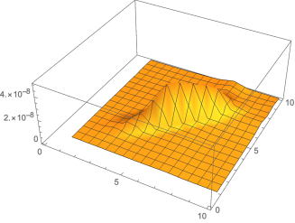
Figure 3: $\bigl{|}1-\frac{{\cal A}^{zz}_{\rm new}}{{\cal A}^{zz}_{\rm old}}\bigr{|}$ for $q=0.5,k=0,\ell=2$.

The maximum value of the relative difference is $\sim 3\times 10^{-8}$. We thus conclude that they agree with rather nice precision and that the discretization scheme proposed in [6] is numerically efficient in our case.

6 The isotropic limit

The isotropic point $\Delta=1$, $h=0$ of the ground state phase diagram of the XXZ chain is located at the boundary between the antiferromagnetic massive and massless regimes (see Figure 1). It can be accessed from the antiferromagnetic massive regime, e.g. by first sending $h\rightarrow 0$ and then $\gamma\rightarrow 0$. The first limit is trivial at zero temperature, since in this case the correlation functions are independent of the magnetic field. The isotropic limit requires a rescaling of the integration variables $u,v\rightarrow\gamma u,\gamma v$. Sending $\gamma\rightarrow 0$ means sending $q\rightarrow 1$. In this limit the functions of the $q$-gamma family become functions of the ordinary gamma family, e.g. $\lim_{q\rightarrow 1}\Gamma_{q}(u)=\Gamma(u)$ and $\lim_{q\rightarrow 1}G_{q}(u)=G(u)$. For those functions involving Jacobi theta functions the limit can be easily calculated after employing a special modular transformation,

$$\vartheta_{1}(\lambda|q) =-{\rm i}\sqrt{\frac{\pi}{\gamma}}\operatorname{e}^{-\frac{\lambda^{2}}{\gamma}}\vartheta_{1}\bigl{(}{\textstyle\frac{\pi{\rm i}\lambda}{\gamma}}\big{|}q^{\prime}\bigr{)}\,, \vartheta_{2}(\lambda|q) =\sqrt{\frac{\pi}{\gamma}}\operatorname{e}^{-\frac{\lambda^{2}}{\gamma}}\vartheta_{4}\bigl{(}{\textstyle\frac{\pi{\rm i}\lambda}{\gamma}}\big{|}q^{\prime}\bigr{)}\,,$$

$$\vartheta_{3}(\lambda|q) =\sqrt{\frac{\pi}{\gamma}}\operatorname{e}^{-\frac{\lambda^{2}}{\gamma}}\vartheta_{3}\bigl{(}{\textstyle\frac{\pi{\rm i}\lambda}{\gamma}}\big{|}q^{\prime}\bigr{)}\,, \vartheta_{4}(\lambda|q) =\sqrt{\frac{\pi}{\gamma}}\operatorname{e}^{-\frac{\lambda^{2}}{\gamma}}\vartheta_{2}\bigl{(}{\textstyle\frac{\pi{\rm i}\lambda}{\gamma}}\big{|}q^{\prime}\bigr{)}\,,$$ (277)

where

$$q^{\prime}=\operatorname{e}^{-\frac{\pi^{2}}{\gamma}}\,.$$ (278)

We indicate the isotropic limit by putting a hat over the respective function, $\hat{f}(u)=\lim_{\gamma\rightarrow 0}f(\gamma u)$. Then the momentum and dressed energy go to

$$\hat{p}(u)=\frac{\pi}{2}-{\rm i}\ln\biggl{(}\frac{\operatorname{ch}\bigl{(}\frac{\pi}{2}(u+\frac{{\rm i}}{2})\bigr{)}}{\operatorname{ch}\bigl{(}\frac{\pi}{2}(u-\frac{{\rm i}}{2})\bigr{)}}\biggr{)}\,,\quad\hat{\varepsilon}(u|0)=-\frac{2\pi J}{\operatorname{ch}(\pi u)}\,.$$ (279)

The function $\Psi$ becomes

$$\hat{\Psi}(u)=\Gamma\bigl{(}{\textstyle\frac{1}{2}}-{\textstyle\frac{{\rm i}u}{2}}\bigr{)}\Gamma\bigl{(}1-{\textstyle\frac{{\rm i}u}{2}}\bigr{)}\frac{G^{2}\bigl{(}1-{\textstyle\frac{{\rm i}u}{2}}\bigr{)}}{G^{2}\bigl{(}\frac{1}{2}-{\textstyle\frac{{\rm i}u}{2}}\bigr{)}}\,.$$ (280)

Severe simplifications of the series in the isotropic limit arise from the theta-function factors. First of all, as is well known, the staggered polarization vanishes in this limit, $\vartheta_{1}^{\prime}/\vartheta_{2}\rightarrow 0$. Moreover,

$$\frac{\vartheta_{2}(\Sigma_{0})}{\vartheta_{2}}\biggr{|}_{\alpha=0}\rightarrow\begin{cases}1&\text{for $k=0$}\\ 0&\text{for $k=1$,}\end{cases}$$ (281)

implying that the whole ‘staggered part’ of the series (246) vanishes for $\gamma\rightarrow 0$, since the remaining factors for $k=1$ have a finite limit. For this reason is enough to give an explicit description of these remaining factors only for $k=0$. If we denote

$$\hat{\Omega}(u,v|{\cal U},{\cal V}) =\lim_{\gamma\rightarrow 0}\gamma\,\Omega(\gamma u,\gamma v|\gamma{\cal U},\gamma{\cal V})\bigr{|}_{k=0,\,\alpha=0}\,,$$ (282a)

$$\hat{\overline{\Omega}}(u,v|{\cal U},{\cal V}) =\lim_{\gamma\rightarrow 0}\gamma\,\overline{\Omega}(\gamma u,\gamma v|\gamma{\cal U},\gamma{\cal V})\bigr{|}_{k=0,\,\alpha=0}\,,$$ (282b)

then

$$\hat{\Omega}(u,v|{\cal U},{\cal V}) =\hat{g}(u,v)-\int_{-\infty}^{\infty}\frac{{\rm d}t}{2\pi{\rm i}}\frac{\hat{\phi}^{(-)}(v)}{\hat{\phi}^{(+)}(t)}\hat{g}(u,t)\hat{\operatorname{e}}(t-v)\,,$$ (283a)

$$\hat{\overline{\Omega}}(v,u|{\cal U},{\cal V}) =\hat{g}(v,u)-\int_{-\infty}^{\infty}\frac{{\rm d}t}{2\pi{\rm i}}\frac{\hat{\phi}^{(-)}(t)}{\hat{\phi}^{(+)}(u)}\hat{g}(v,t)\hat{\operatorname{e}}(u-t)\,,$$ (283b)

where

$$\hat{g}(u,v) =\frac{\pi}{\operatorname{sh}\bigl{(}\pi(v-u)\bigr{)}}\,,\quad\hat{\operatorname{e}}(u)=\frac{1}{u}-\frac{1}{u-{\rm i}}\,,$$ (284a)

$$\phi^{(\sigma)}(u) =\prod_{w\in{\cal U}\ominus{\cal V}}\Gamma\Bigl{(}{\textstyle\frac{1}{2}-\frac{\sigma{\rm i}(u-w)}{2}}\Bigr{)}\Gamma\Bigl{(}{\textstyle 1+\frac{\sigma{\rm i}(u-w)}{2}}\Bigr{)}\,,\quad\sigma=\pm\,.$$ (284b)

For $j=1,\dots,\ell$ we further define

$$\hat{\Omega}^{\rm mod}(u_{j},v_{k}|{\cal U},{\cal V}) =\begin{cases}\int_{-\infty}^{\infty}\frac{{\rm d}t}{\pi}\frac{\hat{\phi}^{(-)}(v_{k})}{\hat{\phi}^{(+)}(t)}\frac{\hat{g}(u_{j},t)}{v_{k}-t}&\text{for $k=1$,}\\[6.45831pt] \hat{\Omega}(u_{j},v_{k}|{\cal U},{\cal V})&\text{for $k=2,\dots,\ell$,}\end{cases}$$ (285a)

$$\hat{\overline{\Omega}}\raisebox{10.0pt}{}^{\rm mod}(v_{j},u_{k}|{\cal U},{\cal V}) =\begin{cases}\int_{-\infty}^{\infty}\frac{{\rm d}t}{\pi}\frac{\hat{\phi}^{(-)}(t)}{\hat{\phi}^{(+)}(u_{k})}\frac{\hat{g}(v_{j},t)}{u_{k}-t}&\text{for $k=1$,}\\[6.45831pt] \hat{\overline{\Omega}}(v_{j},u_{k}|{\cal U},{\cal V})&\text{for $k=2,\dots,\ell$.}\end{cases}$$ (285b)

Inserting all of the above into equation (246) we have arrived at the following theorem.

Theorem 4.

Two-point functions in the isotropic limit.
The dynamical two-point correlation functions of the isotropic Heisenberg chain in the zero-temperature limit have the form factor series representation

$$\bigl{\langle}\sigma_{1}^{z}\sigma_{m+1}^{z}(t)\bigr{\rangle}=\sum_{\ell\in{\mathbb{N}}}\frac{(-1)^{\ell-1}}{((\ell-1)!)^{2}}\int_{\hat{\cal C}_{h}^{\ell}}\frac{{\rm d}^{\ell}u}{(2\pi)^{\ell}}\int_{\hat{\cal C}_{p}^{\ell}}\frac{{\rm d}^{\ell}v}{(2\pi)^{\ell}}\>\operatorname{e}^{-{\rm i}\sum_{\lambda\in{\cal U}\ominus{\cal V}}(m\hat{p}(\lambda)+t\hat{\varepsilon}(\lambda|h))}\\[4.30554pt] \times\sin^{2}\biggl{\{}\sum_{\lambda\in{\cal U}\ominus{\cal V}}\frac{\hat{p}(\lambda)}{2}\biggr{\}}\biggl{[}\prod_{\lambda,\mu\in{\cal U}\ominus{\cal V}}\mspace{-18.0mu}\hat{\Psi}(\lambda-\mu)\biggr{]}\\[4.30554pt] \times\det_{\ell}\{\hat{\Omega}^{\rm mod}(u_{j},v_{k}|{\cal U},{\cal V})\}\det_{\ell}\{\hat{\overline{\Omega}}\raisebox{10.0pt}{}^{\rm mod}(v_{j},u_{k}|{\cal U},{\cal V})\}\,,$$ (286)

where $\hat{\cal C}_{p}={\mathbb{R}}+\frac{{\rm i}(1+0_{+})}{2}$, $\hat{\cal C}_{h}={\mathbb{R}}-\frac{{\rm i}(1+0_{-})}{2}$.

7 Conclusions

We have obtained novel form factor series representations for the longitudinal two-point correlation functions of the XXZ chain in the antiferromagnetic massive regime and of the XXX chain at vanishing magnetic field. These series take simple forms at $T=0$. They are series of multiple integrals of increasing even multiplicity, 2, 4, 6, …. In previous works the integrands in the general terms were of rather intricate forms. They consisted either of sums of multiple contour integrals with complicated contours [35], of sums over multiple residues [16], or, in the best case [18], of functions involving Fredholm determinants in their definition. In the present work the integrands in the $2\ell$-fold integrals are basically products of two order-$\ell$ determinants with entries that can be represented as simple integrals over special functions from the $q$-gamma family.

Expressions for form factors not involving multiple integrals or Fredholm determinants were known for a long time for massive integrable quantum field theories [61], where they had been obtained as solutions of functional equations [62]. They also appear in the context of the Fermionic basis approach to the form factors of the Sine-Gordon model [37]. Thus, taken the close relationship between the XXZ and Sine-Gordon models, the existence of a form factor series for the correlation functions of the XXZ chain in the antiferromagnetic massive regime with form factors represented as finite determinants might have been anticipated. We wish to stress, however, that we have used an eigenbasis of the quantum transfer matrix rather than the Hamiltonian eigenbasis. For this reason our form factor series comes with a different interpretation of the particle content of the model, which is in terms of particles and holes rather than in terms of spinons. The latter are usually interpreted as a lattice manifestation of the quantum solitons in the Sine-Gordon model. This may mean that our representation is still structurally different from everything we would expect to obtain by analogy with the Sine-Gordon model.

We recently learned about a thesis [52] in which a representation of the form factor amplitudes involving only finite determinants was obtained in an eigenbasis of the Hamiltonian of the XXX chain. It will be interesting to see, if that representation can be brought to a more explicit form and how it then compares with our result.

Due to the relative simplicity of our novel expressions, answers to a number of longstanding questions appear now within reach and new questions can be asked.

1. We believe that the novel expressions are more efficient for a numerical computation of the correlation functions.

2. We hope that we will be able to prove the convergence of the series employing methods that were recently developed in the context of integrable massive quantum field theories [51].

3. We hope that we can now attack the problem of calculating the long-time, large-distance asymptotics of two-point correlations in the XXX chain, which requires to estimate all terms in the series as they all contribute.

4. We think that the new series representation may make it possible to prove our older conjecture [18] about the connection of the form factor amplitudes in the spinon and particle-hole bases.

5. As the elements of the matrices $\Omega$ and $\overline{\Omega}$ can be entirely expressed in terms of basic hypergeometric functions the question arises, if there are even more simple and explicit expressions for the corresponding determinants in the general case. The exploration of this question may take us deep into the theory of basic hypergeometric series and may potentially yield new identities between basic hypergeometric series or new derivations of some of the known identities.

In future work we would also like to gain a better understanding of the generic finite temperature case and of the high-$T$ asymptotics. We would further like to explore the possibility if similar series representations exist for the two-point functions in the massless regime. This will require a better understanding of the spectrum and general Bethe root patterns of the excited states of the quantum transfer matrix of the XXZ chain.

Acknowledgments. We would like to thank Jesko Sirker for providing his DMRG data for comparison and Ole Warnaar for helpful discussions about basic hypergeometric series identities. CB and FG acknowledge financial support by the DFG in the framework of the research unit FOR 2316. The work of KKK is supported by the CNRS and by the ‘Projet international de coopération scientifique No. PICS07877’: Fonctions de corrélations dynamiques dans la chaîne XXZ à température finie, Allemagne, 2018-2020. JS is grateful for support by a JSPS Grant-in-Aid for Scientific Research (C) No. 18K03452 and by a JSPS Grant-in-Aid for Scientific Research (B) No. 18H01141.

Note added. While the preparation of this manuscript had been delayed for unforeseeable reasons, we found and proved a generalization to arbitrary $\ell$ of the results of Section 5.3 on the explicit evaluation of the remaining finite determinants in terms of basic hypergeometric series. In order to not further increase the length of the present manuscript, and also for its independent significance, we shall publish this additional result separately.

Appendix A The generating function for the longitudinal two-point function

Here we provide a derivation of equation (30) of the main text. Consider two eigenstates $|l,h\rangle$ and $|n,h\rangle$ of the dynamical quantum transfer matrix $t(\lambda|h)$ which are non-degenerate for $l\neq n$. Then

$$\partial_{h^{\prime}/2T}\langle l,h|t(\lambda|h^{\prime})|n,h^{\prime}\rangle\bigl{|}_{h^{\prime}=h}=\langle l,h|\Sigma^{z}(\lambda|h)|n,h\rangle+\Lambda_{l}(\lambda|h)\langle l,h|\partial_{h/2T}|n,h\rangle\\[4.30554pt] =\delta_{l,n}\langle l,h|l,h\rangle\partial_{h/2T}\Lambda_{n}(\lambda|h)+\Lambda_{n}(\lambda|h)\langle l,h|\partial_{h/2T}|n,h\rangle\,,$$ (A.1)

implying that

$$\langle l,h|\Sigma^{z}(\lambda|h)|n,h\rangle=\\[4.30554pt] \delta_{l,n}\langle l,h|l,h\rangle\partial_{h/2T}\Lambda_{l}(\lambda|h)+\bigl{(}\Lambda_{n}(\lambda|h)-\Lambda_{l}(\lambda|h)\bigr{)}\langle l,h|\partial_{h/2T}|n,h\rangle\,.$$ (A.2)

Similarly,

$$\langle n,h|\Sigma^{z}(\lambda|h)|l,h\rangle=\\[4.30554pt] \delta_{l,n}\langle l,h|l,h\rangle\partial_{h/2T}\Lambda_{l}(\lambda|h)+\bigl{(}\Lambda_{n}(\lambda|h)-\Lambda_{l}(\lambda|h)\bigr{)}\bigl{(}\partial_{h/2T}\langle n,h|\bigr{)}|l,h\rangle\,.$$ (A.3)

Setting $l=0$, multiplying (A.2) and (A.3) and supplying the correct normalization we obtain

$$A_{n}^{zz}=\delta_{n,0}\biggl{(}\frac{\partial_{h/2T}\Lambda(-{\rm i}\gamma/2|h)}{\Lambda(-{\rm i}\gamma/2|h)}\biggr{)}^{2}\\[4.30554pt] +\frac{\langle h|\bigl{(}\partial_{h/2T}|n,h\rangle\bigr{)}\bigl{(}\partial_{h/2T}\langle n,h|\bigr{)}|h\rangle}{\langle h|h\rangle\langle n,h|n,h\rangle}\biggl{(}\frac{\Lambda_{n}(-{\rm i}\gamma/2|h)}{\Lambda(-{\rm i}\gamma/2|h)}-2+\frac{\Lambda(-{\rm i}\gamma/2|h)}{\Lambda_{n}(-{\rm i}\gamma/2|h)}\biggr{)},$$ (A.4)

Now let

$$\varrho_{n}(h^{\prime})=\frac{\langle h|n,h^{\prime}\rangle\langle n,h^{\prime}|h\rangle}{\langle h|h\rangle\langle n,h^{\prime}|n,h^{\prime}\rangle}\,,\quad\varsigma_{n}(h^{\prime})=\frac{\Lambda_{n}(-{\rm i}\gamma/2|h^{\prime})}{\Lambda(-{\rm i}\gamma/2|h)}-2+\frac{\Lambda(-{\rm i}\gamma/2|h)}{\Lambda_{n}(-{\rm i}\gamma/2|h^{\prime})}\,.$$ (A.5)

It follows that

$$\varrho_{0}(h)=1\,,\quad\varsigma_{0}(h)=\varsigma_{0}^{\prime}(h)=0\,,\quad 4T^{2}\varsigma_{0}^{\prime\prime}(h)=2\biggl{(}\frac{\partial_{h/2T}\Lambda(-{\rm i}\gamma/2|h)}{\Lambda(-{\rm i}\gamma/2|h)}\biggr{)}^{2}\,,$$ (A.6)

whereas for $n\neq 0$

$$\varrho_{n}(h)=\varrho_{n}^{\prime}(h)=0\,,\quad 4T^{2}\varrho_{n}^{\prime\prime}(h)=\frac{2\langle h|\bigl{(}\partial_{h/2T}|n,h\rangle\bigr{)}\bigl{(}\partial_{h/2T}\langle n,h|\bigr{)}|h\rangle}{\langle h|h\rangle\langle n,h|n,h\rangle}\,,$$ (A.7)

and $\varsigma_{n}(h)\neq 0$. Thus,

$$2T^{2}\partial_{h^{\prime}}^{2}\varrho_{n}(h^{\prime})\varsigma_{n}(h^{\prime})\bigr{|}_{h^{\prime}=h}=A_{n}^{zz}(h)$$ (A.8)

as a consequence of (A.4), which is equivalent to (30).

Appendix B Determinant of $g_{0}$

In this section we shall derive a product representation of the determinant

$$\Delta_{M}(\mathbf{x},\mathbf{y})=\det_{M}\{g_{0}(x_{j},y_{k})\}\,,$$ (B.1)

where $\mathbf{x}=(x_{1},\dots,x_{M})$, $\mathbf{y}=(y_{1},\dots,y_{M})$. For later convenience we also introduce the notation

$$\mathbf{x}_{l}=(x_{1},\dots,x_{l-1},x_{l+1},\dots,x_{M})$$ (B.2)

and similarly for $\mathbf{y}_{m}$.

Due to the multi-linearity of the determinant, the function $\Delta_{M}(\mathbf{x},\mathbf{y})$ inherits the pole structure and quasi-periodicity from $g_{0}$. In order to understand the latter recall that

$$\vartheta_{1}(x+\pi) =-\vartheta_{1}(x)\,, \vartheta_{1}(x+{\rm i}\gamma)=-q^{-1}\operatorname{e}^{-2{\rm i}x}\vartheta_{1}(x)\,,$$ (B.3a)

$$\vartheta_{2}(x+\pi) =-\vartheta_{2}(x)\,, \vartheta_{2}(x+{\rm i}\gamma)=q^{-1}\operatorname{e}^{-2{\rm i}x}\vartheta_{2}(x)\,.$$ (B.3b)

It follows that

$$g_{0}(x+\pi,y)=g_{0}(x,y)\,,\quad g_{0}(x+{\rm i}\gamma,y)=-g_{0}(x,y)\,.$$ (B.4)

Thus,

$$\Delta_{M}(\mathbf{x}+\pi\mathbf{e}_{l},\mathbf{y})=\Delta_{m}(\mathbf{x},\mathbf{y})\,,\quad\Delta_{M}(\mathbf{x}+{\rm i}\gamma\mathbf{e}_{l},\mathbf{y})=-\Delta_{m}(\mathbf{x},\mathbf{y})\,,$$ (B.5)

where $\mathbf{e}_{l}$ is the $l$th canonical unit vector.

We are looking for a generalization of the Cauchy-det formula. For this reason we define

$$\chi_{M}(\mathbf{x},\mathbf{y})=\frac{\prod_{1\leq j<k\leq M}\vartheta_{1}(x_{j}-x_{k})\vartheta_{1}(y_{k}-y_{j})}{\prod_{j,k=1}^{M}\vartheta_{1}(y_{j}-x_{k})}\,.$$ (B.6)

Then, by (B.3a),

$$\chi_{M}(\mathbf{x}+\pi\mathbf{e}_{l},\mathbf{y}) =-\chi_{M}(\mathbf{x},\mathbf{y})\,,$$ (B.7a)

$$\chi_{M}(\mathbf{x}+{\rm i}\gamma\mathbf{e}_{l},\mathbf{y}) =-q\operatorname{e}^{2{\rm i}\sum_{j=1}^{M}(x_{j}-y_{j})}\chi_{M}(\mathbf{x},\mathbf{y})\,.$$ (B.7b)

We note that $\Delta_{M}$ is an elliptic function (with periods $\pi$, $2{\rm i}\gamma$) in every $x_{l}$. As a function of $x_{l}$ it therefore has as many poles as zeros per cell. The same is definitively not true for $\chi_{M}$. $\chi_{M}$ cannot be elliptic as it has less zeros than poles per cell. Also

$$\Delta_{1}(x,y)=g_{0}(x,y)=\frac{\vartheta_{1}^{\prime}\vartheta_{2}(y-x)}{\vartheta_{2}\vartheta_{1}(y-x)}\,,\quad\chi_{1}(x,y)=\frac{1}{\vartheta_{1}(y-x)}\,.$$ (B.8)

This suggests to replace $\chi_{M}(\mathbf{x},\mathbf{y})$ by

$$\Phi_{M}(\mathbf{x},\mathbf{y})=\vartheta_{2}\bigl{(}{\textstyle\sum_{j=1}^{M}(x_{j}-y_{j})}\bigr{)}\chi_{M}(\mathbf{x},\mathbf{y})\,,$$ (B.9)

which for all $l=1,\dots,M$ has the periodicity properties

$$\Phi_{M}(\mathbf{x}+\pi\mathbf{e}_{l},\mathbf{y})=\Phi_{M}(\mathbf{x},\mathbf{y})\,,\quad\Phi_{M}(\mathbf{x}+{\rm i}\gamma\mathbf{e}_{l},\mathbf{y})=-\Phi_{M}(\mathbf{x},\mathbf{y})$$ (B.10)

following from (B.3b) and (B.7).

We infer that the function

$${\cal F}_{M}(\mathbf{x},\mathbf{y})=\frac{\Delta_{M}(\mathbf{x},\mathbf{y})}{\Phi_{M}(\mathbf{x},\mathbf{y})}$$ (B.11)

is double periodic with periods $\pi$, ${\rm i}\gamma$ and meromorphic in every $x_{l}$, $l=1,\dots,M$, hence an elliptic function of $x_{l}$ with periods $\pi$, ${\rm i}\gamma$. ${\cal F}_{M}$ as a function of $x_{l}$ has at most a single simple pole congruent to $\sum_{j=1}^{M}y_{j}-\sum_{j=1,j\neq l}^{M}x_{j}-\pi/2$ per cell. But such an elliptic function must be a constant, since the sum of the residua of an elliptic function at its poles in any cell is zero. It follows that ${\cal F}_{M}(\mathbf{x},\mathbf{y})$ is independent of $\mathbf{x}$. Repeating all the arguments for $\mathbf{y}$ instead of $\mathbf{x}$, we see that ${\cal F}_{M}(\mathbf{x},\mathbf{y})$ is independent of $\mathbf{y}$ as well, so it is a mere constant.

This constant can be calculated, e.g., by comparing the residua of $\Delta_{M}$ and $\Phi_{M}$ at $x_{l}=y_{k}$. This way we see that ${\cal F}_{M}=(\vartheta_{1}^{\prime})^{M}/\vartheta_{2}$. Thus,

$$\Delta_{M}(\mathbf{x},\mathbf{y})=\frac{\vartheta_{2}(\Sigma)}{\vartheta_{2}}\frac{\prod_{1\leq j<k\leq M}\bigl{(}\vartheta_{1}(x_{j}-x_{k})/\vartheta_{1}^{\prime}\bigr{)}\bigl{(}\vartheta_{1}(y_{k}-y_{j})/\vartheta_{1}^{\prime}\bigr{)}}{\prod_{j,k=1}^{M}\bigl{(}\vartheta_{1}(y_{j}-x_{k})/\vartheta_{1}^{\prime}\bigr{)}}\,,$$ (B.12)

where we have introduced the shorthand notation $\Sigma=\sum_{j=1}^{M}(x_{j}-y_{j})$.

References

• [1] R. J. Baxter, Spontaneous staggered polarization of the ${F}$-model, J. Stat. Phys. 9 (1973), 145.
• [2]  , Corner transfer matrices of the eight-vertex model. I. low-temperature expansions and conjectured properties, J. Stat. Phys. 15 (1976), 485.
• [3] S. Belliard and N. A. Slavnov, Why scalar products in the algebraic Bethe ansatz have determinant representation, J. High Energ. Phys. (2019), 103.
• [4] D. Biegel, M. Karbach, and G. Müller, Transition rates via Bethe ansatz for the spin-$\frac{1}{2}$ Heisenberg chain, Europhys. Lett. 59 (2002), 882.
• [5] H. Boos and F. Göhmann, On the physical part of the factorized correlation functions of the XXZ chain, J. Phys. A 42 (2009), 315001.
• [6] F. Bornemann, On the numerical evaluation of Fredholm determinants, Mathematics of Computation 79 (2010), 871.
• [7] A. H. Bougourzi, M. Couture, and M. Kacir, Exact two-spinon dynamical correlation function of the Heisenberg model, Phys. Rev. B 54 (1996), R12669.
• [8] A. H. Bougourzi, M. Karbach, and G. Müller, Exact two-spinon dynamic structure factor of the one-dimensional $s=1/2$ Heisenberg-Ising antiferromagnet, Phys. Rev. B 57 (1998), 11429.
• [9] J.-S. Caux and R. Hagemans, The 4-spinon dynamical structure factor of the Heisenberg chain, J. Stat. Mech.: Theor. Exp. (2006), P12013.
• [10] J.-S. Caux, H. Konno, M. Sorrell, and R. Weston, Exact form-factor results for the longitudinal structure factor of the massless XXZ model in zero field, J. Stat. Mech.: Theor. Exp. (2012), P01007.
• [11] J.-S. Caux and J. M. Maillet, Computation of dynamical correlation functions of Heisenberg chains in a field, Phys. Rev. Lett. 95 (2005), 077201.
• [12] J.-S. Caux, J. Mossel, and I. Pérez Castillo, The two-spinon transverse structure factor of the gapped Heisenberg antiferromagnetic chain, J. Stat. Mech.: Theor. Exp. (2008), P08006.
• [13] F. Colomo, A. G. Izergin, V. E. Korepin, and V. Tognetti, Correlators in the Heisenberg XXO chain as Fredholm determinants, Phys. Lett. A 169 (1992), 243.
• [14] M. Dugave, F. Göhmann, and K. K. Kozlowski, Thermal form factors of the XXZ chain and the large-distance asymptotics of its temperature dependent correlation functions, J. Stat. Mech.: Theor. Exp. (2013), P07010.
• [15] M. Dugave, F. Göhmann, K. K. Kozlowski, and J. Suzuki, Low-temperature spectrum of correlation lengths of the XXZ chain in the antiferromagnetic massive regime, J. Phys. A 48 (2015), 334001.
• [16]  , On form factor expansions for the XXZ chain in the massive regime, J. Stat. Mech.: Theor. Exp. (2015), P05037.
• [17]  , Asymptotics of correlation functions of the Heisenberg-Ising chain in the easy-axis regime, J. Phys. A 49 (2016), 07LT01.
• [18]  , Thermal form factor approach to the ground-state correlation functions of the XXZ chain in the antiferromagnetic massive regime, J. Phys. A 49 (2016), 394001.
• [19] F. G. Frobenius, Über die elliptischen Functionen zweiter Art, J. Reine Angew. Math. 93 (1882), 53–68.
• [20] G. Gasper and M. Rahman, Basic hypergeometric series, scd. ed., Encyclopedia of Mathematics and its Applications, vol. 96, Cambridge University Press, 2004.
• [21] F. Göhmann, S. Goomanee, K. K. Kozlowski, and J. Suzuki, Thermodynamics of the spin-1/2 Heisenberg-Ising chain at high temperatures: a rigorous approach, Comm. Math. Phys. 377 (2020), 623–673.
• [22] F. Göhmann, M. Karbach, A. Klümper, K. K. Kozlowski, and J. Suzuki, Thermal form-factor approach to dynamical correlation functions of integrable lattice models, J. Stat. Mech.: Theor. Exp. (2017), 113106.
• [23] F. Göhmann, A. Klümper, and A. Seel, Integral representations for correlation functions of the XXZ chain at finite temperature, J. Phys. A 37 (2004), 7625.
• [24]  , Integral representation of the density matrix of the XXZ chain at finite temperature, J. Phys. A 38 (2005), 1833.
• [25] F. Göhmann, K. K. Kozlowski, J. Sirker, and J. Suzuki, Equilibrium dynamics of the XX chain, Phys. Rev. B 100 (2019), 155428.
• [26] F. Göhmann, K. K. Kozlowski, and J. Suzuki, High-temperature analysis of the transverse dynamical two-point correlation function of the XX quantum-spin chain, J. Math. Phys. 61 (2020), 013301.
• [27]  , Long-time large-distance asymptotics of the transversal correlation functions of the XX chain in the space-like regime, Lett. Math. Phys. 110 (2020), 1783–1797.
• [28] E. Granet, M. Fagotti, and F. H. L. Essler, Finite temperature and quench dynamics in the Transverse Field Ising Model from form factor expansions, SciPost Phys. 9 (2020), 33.
• [29] A. Imambekov, T. L. Schmidt, and L. I. Glazman, One-dimensional quantum liquids: Beyond the Luttinger liquid paradigm, Rev. Mod. Phys. 84 (2012), 1253.
• [30] N. Iorgov, Form factors of the finite quantum XY-chain, J. Phys. A 44 (2011), 335005.
• [31] N. Iorgov and O. Lisovyy, Finite-lattice form factors in free-fermion models, J. Stat. Mech.: Theor. Exp. 2011 (2011), P04011.
• [32] A. R. Its, A. G. Izergin, V. E. Korepin, and N. Slavnov, Temperature correlations of quantum spins, Phys. Rev. Lett. 70 (1993), 1704–1706.
• [33] A. G. Izergin, N. Kitanine, J. M. Maillet, and V. Terras, Spontaneous magnetization of the XXZ Heisenberg spin-$\frac{1}{2}$ chain, Nucl. Phys. B 554 (1999), 679.
• [34] X. Jie, The large time asymptotics of the temperature correlation functions of the XX0 Heisenberg ferromagnet: The Riemann-Hilbert approach, Ph.D. thesis, Indiana University Purdue University Indianapolis, 1998.
• [35] M. Jimbo and T. Miwa, Algebraic analysis of solvable lattice models, American Mathematical Society, 1995.
• [36] M. Jimbo, T. Miwa, and F. Smirnov, Hidden Grassmann structure in the XXZ model III: introducing Matsubara direction, J. Phys. A 42 (2009), 304018.
• [37]  , Fermionic structure in the sine-Gordon model: form factors and null-vectors, Nucl. Phys. B 852 (2011), 390.
• [38] M. Karbach, G. Müller, A. H. Bougourzi, A. Fledderjohann, and K.-H. Mütter, Two-spinon dynamic structure factor of the one-dimensional $s=1/2$ Heisenberg antiferromagnet, Phys. Rev. B 55 (1997), 12510.
• [39] N. Kitanine, K. K. Kozlowski, J. M. Maillet, N. A. Slavnov, and V. Terras, On the thermodynamic limit of form factors in the massless XXZ Heisenberg chain, J. Math. Phys. 50 (2009), 095209.
• [40]  , A form factor approach to the asymptotic behavior of correlation functions in critical models, J. Stat. Mech.: Theor. Exp. (2011), P12010.
• [41]  , The thermodynamic limit of particle-hole form factors in the massless XXZ Heisenberg chain, J. Stat. Mech.: Theor. Exp. (2011), P05028.
• [42]  , Form factor approach to dynamical correlation functions in critical models, J. Stat. Mech.: Theor. Exp. (2012), P09001.
• [43] N. Kitanine and G. Kulkarni, Thermodynamic limit of the two-spinon form factors for the zero field XXX chain, SciPost Phys. 6 (2019), 076.
• [44] N. Kitanine, J. M. Maillet, and V. Terras, Form factors of the XXZ Heisenberg spin-$\frac{1}{2}$ finite chain, Nucl. Phys. B 554 (1999), 647.
• [45]  , Correlation functions of the XXZ Heisenberg spin-$\frac{1}{2}$ chain in a magnetic field, Nucl. Phys. B 567 (2000), 554.
• [46] A. Klümper, Thermodynamics of the anisotropic spin-1/2 Heisenberg chain and related quantum chains, Z. Phys. B 91 (1993), 507.
• [47] K. K. Kozlowski, Form factors of bound states in the XXZ chain, J. Phys. A 50 (2017), 184002.
• [48]  , On singularities of dynamic response functions in the massless regime of the XXZ spin-1/2 chain, preprint, arXiv:1811.06076, 2018.
• [49]  , On the thermodynamic limit of form factor expansions of dynamical correlation functions in the massless regime of the XXZ spin 1/2 chain, J. Math. Phys. 59 (2018), 091408.
• [50]  , Long-distance and large-time asymptotic behaviour of dynamic correlation functions in the massless regime of the XXZ spin-1/2 chain, J. Math. Phys. 60 (2019), 073303.
• [51]  , On convergence of form factor expansions in the infinite volume quantum Sinh-Gordon model in 1+1 dimensions, preprint, arXiv:2007.01740, 2020.
• [52] G. Kulkarni, Asymptotic analysis of the form-factors of quantum spin chains, Ph.D. thesis, Université de Bourgogne Franche-Comté, ED 533 Carnot-Pasteur, 2020, arXive:2012.02367.
• [53] M. Lashkevich, Free field construction for the eight-vertex model: representation for form factors, Nucl. Phys. B 621 (2002), 587.
• [54] M. Mourigal, M. Enderle, A. Klöpperpieper, J.-S. Caux, A. Stunault, and H. M. Ronnow, Fractional spinon excitations in the quantum Heisenberg antiferromagnetic chain, Nat. Phys. 9 (2013), 435.
• [55] I. Pérez Castillo, The exact two-spinon longitudinal dynamical structure factor of the anisotropic XXZ model, Preprint, arXiv:2005.10729, 2020.
• [56] H. Rosengren and M. Schlosser, Elliptic determinant evaluations and the Macdonald identities for affine root systems, Compositio Math. 142 (2006), 937–961.
• [57] K. Sakai, Dynamical correlation functions of the XXZ model at finite temperature, J. Phys. A 40 (2007), 7523.
• [58] J. Sato, M. Shiroishi, and M. Takahashi, Evaluation of dynamic spin structure factor for the spin-1/2 XXZ chain in a magnetic field, J. Phys. Soc. Jpn. 73 (2004), 3008.
• [59] N. A. Slavnov, Calculation of scalar products of the wave functions and form factors in the framework of the algebraic Bethe ansatz, Teor. Mat. Fiz. 79 (1989), 232.
• [60]  , Non-equal time current correlation function in a one-dimensional Bose gas, Theor. Math. Phys. 82 (1990), 273–282.
• [61] F. A. Smirnov, A general formula for soliton form factors in the quantum sine-Gordon model, J. Phys. A 19 (1986), L575–L578.
• [62]  , Form factors in completely integrable models of quantum field theory, World Scientific, Singapore, 1992.
• [63] J. Suzuki, Y. Akutsu, and M. Wadati, A new approach to quantum spin chains at finite temperature, J. Phys. Soc. Jpn. 59 (1990), 2667.
• [64] M. Suzuki, Transfer-matrix method and Monte Carlo simulation in quantum spin systems, Phys. Rev. B 31 (1985), 2957.
• [65] E. T. Whittaker and G. N. Watson, A course of modern analysis, fourth ed., ch. 21, Cambridge University Press, 1963.