C-Learning: Horizon-Aware Cumulative
Accessibility Estimation

Panteha Naderian, Gabriel Loaiza-Ganem, Harry J. Braviner, Anthony L. Caterini,
Jesse C. Cresswell & Tong Li
Layer 6 AI
{panteha, gabriel, harry, anthony, jesse, tong}@layer6.ai &Animesh Garg
University of Toronto, Vector Institute, Nvidia
garg@cs.toronto.edu
Abstract

Multi-goal reaching is an important problem in reinforcement learning needed to achieve algorithmic generalization. Despite recent advances in this field, current algorithms suffer from three major challenges: high sample complexity, learning only a single way of reaching the goals, and difficulties in solving complex motion planning tasks. In order to address these limitations, we introduce the concept of cumulative accessibility functions, which measure the reachability of a goal from a given state within a specified horizon. We show that these functions obey a recurrence relation, which enables learning from offline interactions. We also prove that optimal cumulative accessibility functions are monotonic in the planning horizon. Additionally, our method can trade off speed and reliability in goal-reaching by suggesting multiple paths to a single goal depending on the provided horizon. We evaluate our approach on a set of multi-goal discrete and continuous control tasks. We show that our method outperforms state-of-the-art goal-reaching algorithms in success rate, sample complexity, and path optimality. Our code is available at https://github.com/layer6ai-labs/CAE, and additional visualizations can be found at https://sites.google.com/view/learning-cae/.

1 Introduction

Multi-goal reinforcement learning tackles the challenging problem of reaching multiple goals, and as a result, is an ideal framework for real-world agents that solve a diverse set of tasks. Despite progress in this field (Kaelbling, 1993; Schaul etย al., 2015; Andrychowicz etย al., 2017; Ghosh etย al., 2019), current algorithms suffer from a set of limitations: an inability to find multiple paths to a goal, high sample complexity, and poor results in complex motion planning tasks. In this paper we propose C๐ถC-learning, a method which addresses all of these shortcomings.

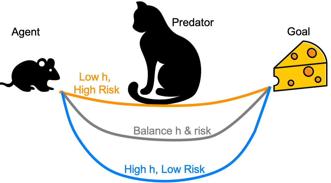
Many multi-goal reinforcement learning algorithms are limited by learning only a single policy ฯ€โ€‹(a|s,g)๐œ‹conditional๐‘Ž๐‘ ๐‘”\pi(a|s,g) over actions a๐‘Ža to reach goal g๐‘”g from state s๐‘ s. There is an unexplored trade-off between reaching the goal reliably and reaching it quickly. We illustrate this shortcoming in Figure 1(a), which represents an environment where an agent must reach a goal on the opposite side of some predator. Shorter paths can reach the goal faster at the cost of a higher probability of being eaten. Existing algorithms do not allow a dynamic choice of whether to act safely or quickly at test time.

The second limitation is sample complexity. Despite significant improvements (Andrychowicz etย al., 2017; Ghosh etย al., 2019), multi-goal reaching still requires a very large amount of environment interactions for effective learning. We argue that the optimal Q๐‘„Q-function must be learned to high accuracy for the agent to achieve reasonable performance, and this leads to sample inefficiency. The same drawback of optimal Q๐‘„Q-functions often causes agents to learn sub-optimal ways of reaching the intended goal. This issue is particularly true for motion planning tasks (Qureshi etย al., 2020), where current algorithms struggle.

We propose to address these limitations by learning horizon-aware policies ฯ€โ€‹(a|s,g,h)๐œ‹conditional๐‘Ž๐‘ ๐‘”โ„Ž\pi(a|s,g,h), which should be followed to reach goal g๐‘”g from state s๐‘ s in at most hโ„Žh steps. The introduction of a time horizon hโ„Žh naturally allows us to tune the speed/reliability trade-off, as an agent wishing to reach the goal faster should select a policy with a suitably small hโ„Žh value. To learn these policies, we introduce the optimal cumulative accessibility function Cโˆ—โ€‹(s,a,g,h)superscript๐ถ๐‘ ๐‘Ž๐‘”โ„ŽC^{*}(s,a,g,h). This is a generalization of the state-action value function and corresponds to the probability of reaching goal g๐‘”g from state s๐‘ s after at most hโ„Žh steps if action a๐‘Ža is taken, and the agent acts optimally thereafter. Intuitively it is similar to the optimal Q๐‘„Q-function, but Q๐‘„Q-functions rarely correspond to probabilities, whereas the Cโˆ—superscript๐ถC^{*}-function does so by construction. We derive Bellman backup update rules for Cโˆ—superscript๐ถC^{*}, which allow it to be learned via minimization of unbiased estimates of the cross-entropy loss โ€“ this is in contrast to Q๐‘„Q-learning, which optimizes biased estimates of the squared error. Policies ฯ€โ€‹(a|s,g,h)๐œ‹conditional๐‘Ž๐‘ ๐‘”โ„Ž\pi(a|s,g,h) can then be recovered from the Cโˆ—superscript๐ถC^{*} function. We call our method cumulative accessibility estimation, or C-learning. Pong etย al. (2018) proposed TDMs, a method involving horizon-aware policies. We point out that their method is roughly related to a non-cumulative version of ours with a different loss that does not enable the speed/reliability trade-off and is ill-suited for sparse rewards. We include a detailed discussion of TDMs in section 4.

One might expect that adding an extra dimension to the learning task, namely hโ„Žh, would increase the difficulty - as Cโˆ—superscript๐ถC^{*} effectively contains the information of several optimal Q๐‘„Q-functions for different discount factors. However, we argue that Cโˆ—superscript๐ถC^{*} does not need to be learned to the same degree of accuracy as the optimal Q๐‘„Q-function for the agent to solve the task. As a result, learning Cโˆ—superscript๐ถC^{*} is more efficient, and converges in fewer environmental interactions. This property, combined with our proposed goal sampling technique and replay buffer used during training, provides empirical improvements over Q๐‘„Q-function based methods.

In addition to these advantages, learning Cโˆ—superscript๐ถC^{*} is itself useful, containing information that the horizon-aware policies do not. It estimates whether a goal g๐‘”g is reachable from the current state s๐‘ s within hโ„Žh steps. In contrast, ฯ€โ€‹(a|s,g,h)๐œ‹conditional๐‘Ž๐‘ ๐‘”โ„Ž\pi(a|s,g,h) simply returns some action, even for unreachable goals. We show that Cโˆ—superscript๐ถC^{*} can be used to determine reachability with examples in a nonholonomic environment.
Refer to caption
(a)
Refer to caption
(b)
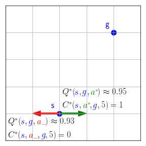
Figure 1: (a)๐‘Ž(a) A continuous spectrum of paths allow the mouse to reach its goal faster, at an increased risk of disturbing the cat and being eaten. (b)๐‘(b) Qโˆ—superscript๐‘„Q^{*} (with ฮณ=0.99๐›พ0.99\gamma=0.99) needs to be learned more accurately than Cโˆ—superscript๐ถC^{*} to act optimally. The goal g๐‘”g can be reached in hโˆ—=5superscriptโ„Ž5h^{*}=5 steps from s๐‘ s, so that Qโˆ—โ€‹(s,g,aโˆ—)=0.995superscript๐‘„๐‘ ๐‘”superscript๐‘Žsuperscript0.995Q^{*}(s,g,a^{*})=0.99^{5} and Qโˆ—โ€‹(s,g,aโˆ’)=0.997superscript๐‘„๐‘ ๐‘”subscript๐‘Žsuperscript0.997Q^{*}(s,g,a_{-})=0.99^{7}; while Cโˆ—โ€‹(s,aโˆ—,g,hโˆ—)=1superscript๐ถ๐‘ superscript๐‘Ž๐‘”superscriptโ„Ž1C^{*}(s,a^{*},g,h^{*})=1 and Cโˆ—โ€‹(s,aโˆ’,g,hโˆ—)=0superscript๐ถ๐‘ subscript๐‘Ž๐‘”superscriptโ„Ž0C^{*}(s,a_{-},g,h^{*})=0.

Summary of contributions: (i)๐‘–(i) introducing C๐ถC-functions and cumulative accessibility estimation for both discrete and continuous action spaces; (iโ€‹i)๐‘–๐‘–(ii) highlighting the importance of the speed vs reliability trade-off in finite horizon reinforcement learning; (iโ€‹iโ€‹i)๐‘–๐‘–๐‘–(iii) introducing a novel replay buffer specially tailored for learning Cโˆ—superscript๐ถC^{*} which builds on HER (Andrychowicz etย al., 2017); and (iโ€‹v)๐‘–๐‘ฃ(iv) empirically showing the effectiveness of our method for goal-reaching as compared to existing alternatives, particularly in the context of complex motion planning tasks.

2 Background and related work

Let us extend the Markov Decision Process (MDP) formalism (Sutton etย al., 1998) for goal-reaching. We consider a set of actions ๐’œ๐’œ\mathcal{A}, a state space ๐’ฎ๐’ฎ\mathcal{S}, and a goal set ๐’ข๐’ข\mathcal{G}. We assume access to a goal checking function G:๐’ฎร—๐’ขโ†’{0,1}:๐บโ†’๐’ฎ๐’ข01G:\mathcal{S}\times\mathcal{G}\rightarrow\{0,1\} such that Gโ€‹(s,g)=1๐บ๐‘ ๐‘”1G(s,g)=1 if and only if state s๐‘ s achieves goal g๐‘”g. For example, achieving the goal could mean exactly reaching a certain state, in which case ๐’ข=๐’ฎ๐’ข๐’ฎ\mathcal{G}=\mathcal{S} and Gโ€‹(s,g)=๐Ÿ™โ€‹(s=g)๐บ๐‘ ๐‘”1๐‘ ๐‘”G(s,g)=\mathds{1}(s=g). For many continuous state-spaces, hitting a state exactly has zero probability. Here we can still take ๐’ข=๐’ฎ๐’ข๐’ฎ\mathcal{G}=\mathcal{S}, but let Gโ€‹(s,g)=๐Ÿ™โ€‹(dโ€‹(s,g)โ‰คฯต)๐บ๐‘ ๐‘”1๐‘‘๐‘ ๐‘”italic-ฯตG(s,g)=\mathds{1}(d(s,g)\leq\epsilon) for some radius ฯตitalic-ฯต\epsilon and metric d๐‘‘d. More general choices are possible. For example, in the Dubinsโ€™ Car environment which we describe in more detail later, the state consists of both the location and orientation of the car: ๐’ฎ=โ„2ร—S1๐’ฎsuperscriptโ„2superscript๐‘†1\mathcal{S}=\mathbb{R}^{2}\times S^{1}. We take ๐’ข=โ„2๐’ขsuperscriptโ„2\mathcal{G}=\mathbb{R}^{2}, and Gโ€‹(s,g)๐บ๐‘ ๐‘”G(s,g) checks that the location of the car is within some small radius of g๐‘”g, ignoring the direction entirely. For a fixed g๐‘”g, Gโ€‹(s,g)๐บ๐‘ ๐‘”G(s,g) can be thought of as a sparse reward function.

In the goal-reaching setting, a policy ฯ€:๐’ฎร—๐’ขโ†’๐’ซโ€‹(๐’œ):๐œ‹โ†’๐’ฎ๐’ข๐’ซ๐’œ\pi:\mathcal{S}\times\mathcal{G}\rightarrow\mathcal{P}(\mathcal{A}), where ๐’ซโ€‹(๐’œ)๐’ซ๐’œ\mathcal{P}(\mathcal{A}) denotes the set of distributions over ๐’œ๐’œ\mathcal{A}, maps state-goal pairs to an action distribution. The environment dynamics are given by a starting distribution pโ€‹(s0,g)๐‘subscript๐‘ 0๐‘”p(s_{0},g), usually taken as pโ€‹(s0)โ€‹pโ€‹(g)๐‘subscript๐‘ 0๐‘๐‘”p(s_{0})p(g), and transition probabilities pโ€‹(st+1|st,at)๐‘conditionalsubscript๐‘ ๐‘ก1subscript๐‘ ๐‘กsubscript๐‘Ž๐‘กp(s_{t+1}|s_{t},a_{t}). States for which Gโ€‹(s,g)=1๐บ๐‘ ๐‘”1G(s,g)=1 are considered terminal.

Q-Learning: A Q๐‘„Q-function (Watkins & Dayan, 1992) for multi-goal reaching, Qฯ€:๐’ฎร—๐’ขร—๐’œโ†’โ„:superscript๐‘„๐œ‹โ†’๐’ฎ๐’ข๐’œโ„Q^{\pi}:\mathcal{S}\times\mathcal{G}\times\mathcal{A}\rightarrow\mathbb{R}, is defined by Qฯ€โ€‹(st,g,at)=๐”ผฯ€โ€‹[โˆ‘i=tโˆžฮณiโˆ’tโ€‹Gโ€‹(st,g)|st,at]superscript๐‘„๐œ‹subscript๐‘ ๐‘ก๐‘”subscript๐‘Ž๐‘กsubscript๐”ผ๐œ‹delimited-[]conditionalsuperscriptsubscript๐‘–๐‘กsuperscript๐›พ๐‘–๐‘ก๐บsubscript๐‘ ๐‘ก๐‘”subscript๐‘ ๐‘กsubscript๐‘Ž๐‘กQ^{\pi}(s_{t},g,a_{t})=\mathbb{E}_{\pi}[\sum_{i=t}^{\infty}\gamma^{i-t}G(s_{t},g)|s_{t},a_{t}], where ฮณโˆˆ[0,1]๐›พ01\gamma\in[0,1] is a discount factor and the expectation is with respect to state-action trajectories obtained by using ฯ€โ€‹(a|si,g)๐œ‹conditional๐‘Žsubscript๐‘ ๐‘–๐‘”\pi(a|s_{i},g). If ฯ€โˆ—superscript๐œ‹\pi^{*} is an optimal policy in the sense that Qฯ€โˆ—โ€‹(s,g,a)โ‰ฅQฯ€โ€‹(s,g,a)superscript๐‘„superscript๐œ‹๐‘ ๐‘”๐‘Žsuperscript๐‘„๐œ‹๐‘ ๐‘”๐‘ŽQ^{\pi^{*}}(s,g,a)\geq Q^{\pi}(s,g,a) for every ฯ€๐œ‹\pi and (s,g,a)โˆˆ๐’ฎร—๐’ขร—๐’œ๐‘ ๐‘”๐‘Ž๐’ฎ๐’ข๐’œ(s,g,a)\in\mathcal{S}\times\mathcal{G}\times\mathcal{A}, then Qฯ€โˆ—superscript๐‘„superscript๐œ‹Q^{\pi^{*}} matches the optimal Q๐‘„Q-function, Qโˆ—superscript๐‘„Q^{*}, which obeys the Bellman equation:

Qโˆ—โ€‹(s,g,a)=๐”ผsโ€ฒโˆผp(โ‹…|s,a)โ€‹[Gโ€‹(s,g)+ฮณโ€‹maxaโ€ฒโˆˆ๐’œโกQโˆ—โ€‹(sโ€ฒ,g,aโ€ฒ)].Q^{*}(s,g,a)=\mathbb{E}_{s^{\prime}\sim p(\cdot|s,a)}\left[G(s,g)+\gamma\max_{a^{\prime}\in\mathcal{A}}Q^{*}(s^{\prime},g,a^{\prime})\right]. (1)

In deep Q๐‘„Q-learning (Mnih etย al., 2015), Qโˆ—superscript๐‘„Q^{*} is parameterized with a neural network and learning is achieved by enforcing the relationship from equation 1. This is done by minimizing โˆ‘iโ„’โ€‹(Qโˆ—โ€‹(si,gi,ai),yi)subscript๐‘–โ„’superscript๐‘„subscript๐‘ ๐‘–subscript๐‘”๐‘–subscript๐‘Ž๐‘–subscript๐‘ฆ๐‘–\sum_{i}\mathcal{L}(Q^{*}(s_{i},g_{i},a_{i}),y_{i}), where yisubscript๐‘ฆ๐‘–y_{i} corresponds to the expectation in equation 1 and is estimated using a replay buffer of stored tuples (si,ai,gi,siโ€ฒ)subscript๐‘ ๐‘–subscript๐‘Ž๐‘–subscript๐‘”๐‘–superscriptsubscript๐‘ ๐‘–โ€ฒ(s_{i},a_{i},g_{i},s_{i}^{\prime}). Note that siโ€ฒsubscriptsuperscript๐‘ โ€ฒ๐‘–s^{\prime}_{i} is the state the environment transitioned to after taking action aisubscript๐‘Ž๐‘–a_{i} from state sisubscript๐‘ ๐‘–s_{i}, and determines the value of yisubscript๐‘ฆ๐‘–y_{i}. Typically โ„’โ„’\mathcal{L} is chosen as a squared error loss, and the dependency of yisubscript๐‘ฆ๐‘–y_{i} on Qโˆ—superscript๐‘„Q^{*} is ignored for backpropagation in order to stabilize training. Once Qโˆ—superscript๐‘„Q^{*} is learned, the optimal policy is recovered by ฯ€โˆ—โ€‹(a|s,g)=๐Ÿ™โ€‹(a=argโ€‹maxaโ€ฒโกQโˆ—โ€‹(s,g,aโ€ฒ))superscript๐œ‹conditional๐‘Ž๐‘ ๐‘”1๐‘Žsubscriptargmaxsuperscript๐‘Žโ€ฒsuperscript๐‘„๐‘ ๐‘”superscript๐‘Žโ€ฒ\pi^{*}(a|s,g)=\mathds{1}(a=\operatorname*{arg\,max}_{a^{\prime}}Q^{*}(s,g,a^{\prime})).

There is ample work extending and improving upon deep Q๐‘„Q-learning (Haarnoja etย al., 2018). For example, Lillicrap etย al. (2015) extend it to the continuous action space setting, and Fujimoto etย al. (2018) further stabilize training. These improvements are fully compatible with goal-reaching (Pong etย al., 2019; Bharadhwaj etย al., 2020a; Ghosh etย al., 2019). Andrychowicz etย al. (2017) proposed Hindsight Experience Replay (HER), which relabels past experience as achieved goals, and allows sample efficient learning from sparse rewards (Nachum etย al., 2018).

3 Cumulative accessibility functions

a๐‘Žaa1subscript๐‘Ž1a_{1}a2subscript๐‘Ž2a_{2}a3subscript๐‘Ž3a_{3}s๐‘ shโ„Žhs1subscript๐‘ 1s_{1}hโˆ’1โ„Ž1h-1s2subscript๐‘ 2s_{2}hโˆ’2โ„Ž2h-2s3subscript๐‘ 3s_{3}hโˆ’3โ„Ž3h-3g๐‘”gโ€ฆโ€ฆ

Figure 2: Graphical model depicting trajectories from โ„™ฯ€(โ‹…|โ‹…,g,h)(โ‹…|s0=s,a0=a)\mathbb{P}_{\pi(\cdot|\cdot,g,h)}(\cdot|s_{0}=s,a_{0}=a). Gray nodes denote fixed values, and white nodes stochastic ones. Nodes a๐‘Ža, g๐‘”g and s๐‘ s are non-stochastic simply because they are conditioned on, not because they are always fixed within the environment. Note that the values of hโ„Žh decrease deterministically. Nodes corresponding to horizons could be separated from states, but are not for a more concise graph.

We now consider horizon-aware policies ฯ€:๐’ฎร—๐’ขร—โ„•โ†’๐’ซโ€‹(๐’œ):๐œ‹โ†’๐’ฎ๐’ขโ„•๐’ซ๐’œ\pi:\mathcal{S}\times\mathcal{G}\times\mathbb{N}\rightarrow\mathcal{P}(\mathcal{A}), and define the cumulative accessibility function Cฯ€โ€‹(s,a,g,h)superscript๐ถ๐œ‹๐‘ ๐‘Ž๐‘”โ„ŽC^{\pi}(s,a,g,h), or C๐ถC-function, as the probability of reaching goal g๐‘”g from state s๐‘ s in at most hโ„Žh steps by taking action a๐‘Ža and following the policy ฯ€๐œ‹\pi thereafter. By โ€œfollowing the policy ฯ€๐œ‹\pi thereafterโ€ we mean that after a๐‘Ža, the next action a1subscript๐‘Ž1a_{1} is sampled from ฯ€(โ‹…|s1,g,hโˆ’1)\pi(\cdot|s_{1},g,h-1), a2subscript๐‘Ž2a_{2} is sampled from ฯ€(โ‹…|s2,g,hโˆ’2)\pi(\cdot|s_{2},g,h-2) and so on. See Figure 2 for a graphical model depiction of how these trajectories are obtained. Importantly, an agent need not always act the same way at a particular state in order to reach a particular goal, thanks to horizon-awareness. We use โ„™ฯ€(โ‹…|โ‹…,g,h)(โ‹…|s0=s,a0=a)\mathbb{P}_{\pi(\cdot|\cdot,g,h)}(\cdot|s_{0}=s,a_{0}=a) to denote probabilities in which actions are drawn in this manner and transitions are drawn according to the environment pโ€‹(st+1|st,a)๐‘conditionalsubscript๐‘ ๐‘ก1subscript๐‘ ๐‘ก๐‘Žp(s_{t+1}|s_{t},a). More formally, Cฯ€superscript๐ถ๐œ‹C^{\pi} is given by:

Cฯ€(s,a,g,h)=โ„™ฯ€(โ‹…|โ‹…,g,h)(maxt=0,โ€ฆ,hG(st,g)=1|s0=s,a0=a).C^{\pi}(s,a,g,h)=\mathbb{P}_{\pi(\cdot|\cdot,g,h)}\left(\displaystyle\max_{t=0,\dots,h}G(s_{t},g)=1\middle|s_{0}=s,a_{0}=a\right). (2)

Proposition 1: Cฯ€superscript๐ถ๐œ‹C^{\pi} can be framed as a Q๐‘„Q-function within the MDP formalism, and if ฯ€โˆ—superscript๐œ‹\pi^{*} is optimal in the sense that Cฯ€โˆ—โ€‹(s,a,g,h)โ‰ฅCฯ€โ€‹(s,a,g,h)superscript๐ถsuperscript๐œ‹๐‘ ๐‘Ž๐‘”โ„Žsuperscript๐ถ๐œ‹๐‘ ๐‘Ž๐‘”โ„ŽC^{\pi^{*}}(s,a,g,h)\geq C^{\pi}(s,a,g,h) for every ฯ€๐œ‹\pi and (s,a,g,h)โˆˆ๐’ฎร—๐’œร—๐’ขร—โ„•๐‘ ๐‘Ž๐‘”โ„Ž๐’ฎ๐’œ๐’ขโ„•(s,a,g,h)\in\mathcal{S}\times\mathcal{A}\times\mathcal{G}\times\mathbb{N}, then Cฯ€โˆ—superscript๐ถsuperscript๐œ‹C^{\pi^{*}} matches the optimal C๐ถC-function, Cโˆ—superscript๐ถC^{*}, which obeys the following equation:

Cโˆ—โ€‹(s,a,g,h)={๐”ผsโ€ฒโˆผp(โ‹…|s,a)โ€‹[maxaโ€ฒโˆˆ๐’œโกCโˆ—โ€‹(sโ€ฒ,aโ€ฒ,g,hโˆ’1)]โ€‹ย ifย โ€‹Gโ€‹(s,g)=0โ€‹ย andย โ€‹hโ‰ฅ1,Gโ€‹(s,g)ย otherwise.C^{*}(s,a,g,h)=\begin{cases}\mathbb{E}_{s^{\prime}\sim p(\cdot|s,a)}\left[\displaystyle\max_{a^{\prime}\in\mathcal{A}}C^{*}(s^{\prime},a^{\prime},g,h-1)\right]\text{ if }G(s,g)=0\text{ and }h\geq 1,\\ G(s,g)\hskip 127.0pt\text{ otherwise}.\end{cases} (3)

See appendix A for a detailed mathematical proof of this proposition. The proof proceeds by first deriving a recurrence relationship that holds for any Cฯ€superscript๐ถ๐œ‹C^{\pi}. In an analogous manner to the Bellman equation in Q๐‘„Q-learning, this recurrence involves an expectation over ฯ€(โ‹…|sโ€ฒ,g,hโˆ’1)\pi(\cdot|s^{\prime},g,h-1), which, when replaced by a max\max returns the recursion for Cโˆ—superscript๐ถC^{*}.

Proposition 1 is relevant as it allows us to learn Cโˆ—superscript๐ถC^{*}, enabling goal-reaching policies to be recovered:

ฯ€โˆ—โ€‹(a|s,g,h)=๐Ÿ™โ€‹(a=argโ€‹maxaโ€ฒโกCโˆ—โ€‹(s,aโ€ฒ,g,h)).superscript๐œ‹conditional๐‘Ž๐‘ ๐‘”โ„Ž1๐‘Žsubscriptargmaxsuperscript๐‘Žโ€ฒsuperscript๐ถ๐‘ superscript๐‘Žโ€ฒ๐‘”โ„Ž\pi^{*}(a|s,g,h)=\mathds{1}\left(a=\operatorname*{arg\,max}_{a^{\prime}}C^{*}(s,a^{\prime},g,h)\right). (4)

Cโˆ—superscript๐ถC^{*} itself is useful for determining reachability. After maximizing over actions, it estimates whether a given goal is reachable from a state within some horizon. Comparing these probabilities for different horizons allows us to make a speed / reliability trade-off for reaching goals.

We observe that an optimal Cโˆ—superscript๐ถC^{*}-function is non-decreasing in hโ„Žh, but this does not necessarily hold for non-optimal C๐ถC-functions. For example, a horizon-aware policy could actively try to avoid the goal for high values of hโ„Žh, and the Cฯ€superscript๐ถ๐œ‹C^{\pi}-function constructed from it would show lower probabilities of success for larger hโ„Žh. See appendix A for a concrete example of this counter-intuitive behavior.

Proposition 2: Cโˆ—superscript๐ถC^{*} is non-decreasing in hโ„Žh.
See appendix A for a detailed mathematical proof. Intuitively, the proof consists of showing that an optimal policy can not exhibit the pathology mentioned above. Given an optimal policy ฯ€โˆ—โ€‹(a|s,g,h)superscript๐œ‹conditional๐‘Ž๐‘ ๐‘”โ„Ž\pi^{*}(a|s,g,h) for a fixed horizon hโ„Žh we construct a policy ฯ€~~๐œ‹\tilde{\pi} for h+1โ„Ž1h+1 which always performs better, and lower bounds the performance of ฯ€โˆ—โ€‹(a|s,g,h+1)superscript๐œ‹conditional๐‘Ž๐‘ ๐‘”โ„Ž1\pi^{*}(a|s,g,h+1).

In addition to being an elegant theoretical property, proposition 2 suggests that there is additional structure in a Cโˆ—superscript๐ถC^{*} function which mitigates the added complexity from using horizon-aware policies. Indeed, in our preliminary experiments we used a non-cumulative version of C๐ถC-functions (see section 3.3) and obtained significantly improved performance upon changing to C๐ถC-functions. Moreover, monotonicity in hโ„Žh could be encoded in the architecture of Cโˆ—superscript๐ถC^{*} (Sill, 1998; Wehenkel & Louppe, 2019). However, we found that actively doing so hurt empirical performance (appendix F).

3.1 Shortcomings of Q๐‘„Q-learning

Before describing our method for learning Cโˆ—superscript๐ถC^{*}, we highlight a shortcoming of Q๐‘„Q-learning. Consider a 2D navigation environment where an agent can move deterministically in the cardinal directions, and fix s๐‘ s and g๐‘”g. For an optimal action aโˆ—superscript๐‘Ža^{*}, the optimal Q๐‘„Q function will achieve some value Qโˆ—โ€‹(s,g,aโˆ—)โˆˆ[0,1]superscript๐‘„๐‘ ๐‘”superscript๐‘Ž01Q^{*}(s,g,a^{*})\in[0,1] in the sparse reward setting. Taking a sub-optimal action aโˆ’superscript๐‘Ža^{-} initially results in the agent taking two extra steps to reach the intended goal, given that the agent acts optimally after the first action, so that Qโˆ—โ€‹(s,g,aโˆ’)=ฮณ2โ€‹Qโˆ—โ€‹(s,g,aโˆ—)superscript๐‘„๐‘ ๐‘”superscript๐‘Žsuperscript๐›พ2superscript๐‘„๐‘ ๐‘”superscript๐‘ŽQ^{*}(s,g,a^{-})=\gamma^{2}Q^{*}(s,g,a^{*}). The value of ฮณ๐›พ\gamma is typically chosen close to 111, for example 0.990.990.99, to ensure that future rewards are not too heavily discounted. As a consequence ฮณ2โ‰ˆ1superscript๐›พ21\gamma^{2}\approx 1 and thus the value of Qโˆ—superscript๐‘„Q^{*} at the optimal action is very close to its value at a sub-optimal action. We illustrate this issue in Figure 1(b). In this scenario, recovering an optimal policy requires that the error between the learned Q๐‘„Q-function and Qโˆ—superscript๐‘„Q^{*} should be at most (1โˆ’ฮณ2)/21superscript๐›พ22(1-\gamma^{2})/2; this is reflected empirically by Q๐‘„Q-learning having high sample complexity and learning sub-optimal paths. This shortcoming surfaces in any environment where taking a sub-optimal action results in a slightly longer path than an optimal one, as in e.g.ย motion planning tasks.

The Cโˆ—superscript๐ถC^{*} function does not have this shortcoming. Consider the same 2D navigation example, and let hโˆ—superscriptโ„Žh^{*} be the smallest horizon for which g๐‘”g can be reached from s๐‘ s. hโˆ—superscriptโ„Žh^{*} can be easily obtained from Cโˆ—superscript๐ถC^{*} as the smallest hโ„Žh such that maxaโกCโˆ—โ€‹(s,a,g,h)=1subscript๐‘Žsuperscript๐ถ๐‘ ๐‘Ž๐‘”โ„Ž1\max_{a}C^{*}(s,a,g,h)=1. Again, denoting aโˆ—superscript๐‘Ža^{*} as an optimal action and aโˆ’superscript๐‘Ža^{-} as a sub-optimal one, we have that Cโˆ—โ€‹(s,aโˆ—,g,hโˆ—)=1superscript๐ถ๐‘ superscript๐‘Ž๐‘”superscriptโ„Ž1C^{*}(s,a^{*},g,h^{*})=1 whereas Cโˆ—โ€‹(s,aโˆ’,g,hโˆ—)=0superscript๐ถ๐‘ superscript๐‘Ž๐‘”superscriptโ„Ž0C^{*}(s,a^{-},g,h^{*})=0, which is illustrated in Figure 1(b). Therefore, the threshold for error is much higher when learning the Cโˆ—superscript๐ถC^{*} function. This property results in fewer interactions with the environment needed to learn Cโˆ—superscript๐ถC^{*} and more efficient solutions.

3.2 Horizon-independent policies

Given a Cโˆ—superscript๐ถC^{*}-function, equation 4 lets us recover a horizon-aware policy. At test time, using small values of hโ„Žh can achieve goals faster, while large values of hโ„Žh will result in safe policies. However, a natural question arises: how small is small and how large is large? In this section we develop a method to quantitatively recover reasonable values of hโ„Žh which adequately balance the speed/reliability trade-off. First, a safety threshold ฮฑโˆˆ(0,1]๐›ผ01\alpha\in(0,1] is chosen, which indicates the percentage of the maximum value of Cโˆ—superscript๐ถC^{*} we are willing to accept as safe enough. Smaller values of ฮฑ๐›ผ\alpha will thus result in quicker policies, while larger values will result in safer ones. Then we consider a range of viable horizons, โ„‹โ„‹\mathcal{H}, and find the maximal Cโˆ—superscript๐ถC^{*} value, Mโ€‹(s,g)=maxhโˆˆโ„‹,aโˆˆ๐’œโกCโˆ—โ€‹(s,a,g,h)๐‘€๐‘ ๐‘”subscriptformulae-sequenceโ„Žโ„‹๐‘Ž๐’œsuperscript๐ถ๐‘ ๐‘Ž๐‘”โ„ŽM(s,g)=\max_{h\in\mathcal{H},a\in\mathcal{A}}C^{*}(s,a,g,h). We then compute:

hฮฑโ€‹(s,g)=argโ€‹minhโˆˆโ„‹โก{maxaโˆˆ๐’œโกCโˆ—โ€‹(s,a,g,h):maxaโˆˆ๐’œโกCโˆ—โ€‹(s,a,g,h)โ‰ฅฮฑโ€‹Mโ€‹(s,g)},subscriptโ„Ž๐›ผ๐‘ ๐‘”subscriptargminโ„Žโ„‹:subscript๐‘Ž๐’œsuperscript๐ถ๐‘ ๐‘Ž๐‘”โ„Žsubscript๐‘Ž๐’œsuperscript๐ถ๐‘ ๐‘Ž๐‘”โ„Ž๐›ผ๐‘€๐‘ ๐‘”h_{\alpha}(s,g)=\operatorname*{arg\,min}_{h\in\mathcal{H}}\{\max_{a\in\mathcal{A}}C^{*}(s,a,g,h):\max_{a\in\mathcal{A}}C^{*}(s,a,g,h)\geq\alpha M(s,g)\}, (5)

and take ฯ€ฮฑโˆ—โ€‹(a|s,g)=๐Ÿ™โ€‹(a=argโ€‹maxaโ€ฒโกCโˆ—โ€‹(s,aโ€ฒ,g,hฮฑโ€‹(s,g)))subscriptsuperscript๐œ‹๐›ผconditional๐‘Ž๐‘ ๐‘”1๐‘Žsubscriptargmaxsuperscript๐‘Žโ€ฒsuperscript๐ถ๐‘ superscript๐‘Žโ€ฒ๐‘”subscriptโ„Ž๐›ผ๐‘ ๐‘”\pi^{*}_{\alpha}(a|s,g)=\mathds{1}\left(a=\operatorname*{arg\,max}_{a^{\prime}}C^{*}(s,a^{\prime},g,h_{\alpha}(s,g))\right). This procedure also allows us to recover horizon-independent policies from Cโˆ—superscript๐ถC^{*} by using a fixed value of ฮฑ๐›ผ\alpha, which makes comparing against horizon-unaware methods straightforward. We used horizon-unaware policies with added randomness as the behaviour policy when interacting with the environment for exploration.

3.3 Alternative recursions

One could consider defining a non-cumulative version of the C๐ถC-function, which we call an A๐ดA-function for โ€œaccessibilityโ€ (not for โ€œadvantageโ€), yielding the probability of reaching a goal in exactly hโ„Žh steps. However, this version is more susceptible to pathological behaviors that hinder learning for certain environments. For illustration, consider an agent that must move one step at a time in the cardinal directions on a checkerboard. Starting on a dark square, the probability of reaching a light square in an even number of steps is always zero, but may be non-zero for odd numbers. An optimal A๐ดA-function would fluctuate wildly as the step horizon hโ„Žh is increased, resulting in a harder target to learn. Nonetheless, A๐ดA-functions admit a similar recursion to equationย 18, which we include in appendix C for completeness. In any case, the C๐ถC-function provides a notion of reachability which is more closely tied to related work (Savinov etย al., 2018; Venkattaramanujam etย al., 2019; Ghosh etย al., 2018; Bharadhwaj etย al., 2020a).

In Q๐‘„Q-learning, discount factors close to 111 encourage safe policies, while discount factors close to 00 encourage fast policies. One could then also consider discount-conditioned policies ฯ€โ€‹(a|s,g,ฮณ)๐œ‹conditional๐‘Ž๐‘ ๐‘”๐›พ\pi(a|s,g,\gamma) as a way to achieve horizon-awareness. In appendix D we introduce D๐ทD-functions (for โ€œdiscountโ€), Dโ€‹(s,a,g,ฮณ)๐ท๐‘ ๐‘Ž๐‘”๐›พD(s,a,g,\gamma), which allow recovery of discount-conditioned policies. However D๐ทD-functions suffer from the same limitation as Q๐‘„Q-functions in that they need to be learned to a high degree of accuracy.

4 Cumulative accessibility estimation

Our training algorithm, which we call cumulative accessibility estimation (CAE), or C๐ถC-learning, is detailed in algorithm 1. Similarly to Q๐‘„Q-learning, the Cโˆ—superscript๐ถC^{*} function can be modelled as a neural network with parameters ฮธ๐œƒ\theta, denoted Cฮธโˆ—subscriptsuperscript๐ถ๐œƒC^{*}_{\theta}, which can be learned by minimizing:

โˆ’โˆ‘i[yiโ€‹logโกCฮธโˆ—โ€‹(si,ai,gi,hi)+(1โˆ’yi)โ€‹logโก(1โˆ’Cฮธโˆ—โ€‹(si,ai,gi,hi))],subscript๐‘–delimited-[]subscript๐‘ฆ๐‘–subscriptsuperscript๐ถ๐œƒsubscript๐‘ ๐‘–subscript๐‘Ž๐‘–subscript๐‘”๐‘–subscriptโ„Ž๐‘–1subscript๐‘ฆ๐‘–1subscriptsuperscript๐ถ๐œƒsubscript๐‘ ๐‘–subscript๐‘Ž๐‘–subscript๐‘”๐‘–subscriptโ„Ž๐‘–-\sum_{i}\left[y_{i}\log C^{*}_{\theta}(s_{i},a_{i},g_{i},h_{i})+(1-y_{i})\log\left(1-C^{*}_{\theta}(s_{i},a_{i},g_{i},h_{i})\right)\right], (6)

where yisubscript๐‘ฆ๐‘–y_{i} corresponds to a stochastic estimate of the right hand side of equation 18. The sum is over tuples (si,ai,siโ€ฒ,gi,hi)subscript๐‘ ๐‘–subscript๐‘Ž๐‘–subscriptsuperscript๐‘ โ€ฒ๐‘–subscript๐‘”๐‘–subscriptโ„Ž๐‘–(s_{i},a_{i},s^{\prime}_{i},g_{i},h_{i}) drawn from a replay buffer which we specially tailor to successfully learn Cโˆ—superscript๐ถC^{*}. Since Cโˆ—superscript๐ถC^{*} corresponds to a probability, we change the usual squared loss to be the binary cross entropy loss. Note that even if the targets yisubscript๐‘ฆ๐‘–y_{i} are not necessarily binary, the use of binary cross entropy is still justified as it is equivalent to minimizing the ๐•‚โ€‹๐•ƒ๐•‚๐•ƒ\mathbb{KL} divergence between Bernoulli distributions with parameters yisubscript๐‘ฆ๐‘–y_{i} and Cฮธโˆ—โ€‹(si,ai,gi,hi)superscriptsubscript๐ถ๐œƒsubscript๐‘ ๐‘–subscript๐‘Ž๐‘–subscript๐‘”๐‘–subscriptโ„Ž๐‘–C_{\theta}^{*}(s_{i},a_{i},g_{i},h_{i}) (Bellemare etย al., 2017). Since the targets used do not correspond to the right-hand side of equation 18 but to a stochastic estimate (through siโ€ฒsuperscriptsubscript๐‘ ๐‘–โ€ฒs_{i}^{\prime}) of it, using this loss instead of the square loss results in an unbiased estimate of โˆ‘iโ„’โ€‹(Cฮธโˆ—โ€‹(si,ai,gi,hi),yitrue)subscript๐‘–โ„’superscriptsubscript๐ถ๐œƒsubscript๐‘ ๐‘–subscript๐‘Ž๐‘–subscript๐‘”๐‘–subscriptโ„Ž๐‘–superscriptsubscript๐‘ฆ๐‘–true\sum_{i}\mathcal{L}(C_{\theta}^{*}(s_{i},a_{i},g_{i},h_{i}),y_{i}^{\mathrm{true}}), where yitruesuperscriptsubscript๐‘ฆ๐‘–truey_{i}^{\mathrm{true}} corresponds to the right-hand side of equation 18 at (si,ai,gi,hi)subscript๐‘ ๐‘–subscript๐‘Ž๐‘–subscript๐‘”๐‘–subscriptโ„Ž๐‘–(s_{i},a_{i},g_{i},h_{i}) (see appendix B for a detailed explanation). This confers another benefit of C๐ถC-learning over Q๐‘„Q-learning, as passing a stochastic estimate of equation 1 through the typical squared loss results in biased estimators. As in Double Q๐‘„Q-learning (Vanย Hasselt etย al., 2015), we use a second network Cฮธโ€ฒโˆ—subscriptsuperscript๐ถsuperscript๐œƒโ€ฒC^{*}_{\theta^{\prime}} to compute the yisubscript๐‘ฆ๐‘–y_{i} targets, and do not minimize equation 6 with respect to ฮธโ€ฒsuperscript๐œƒโ€ฒ\theta^{\prime}. We periodically update ฮธโ€ฒsuperscript๐œƒโ€ฒ\theta^{\prime} to match ฮธ๐œƒ\theta. We now explain our algorithmic details.

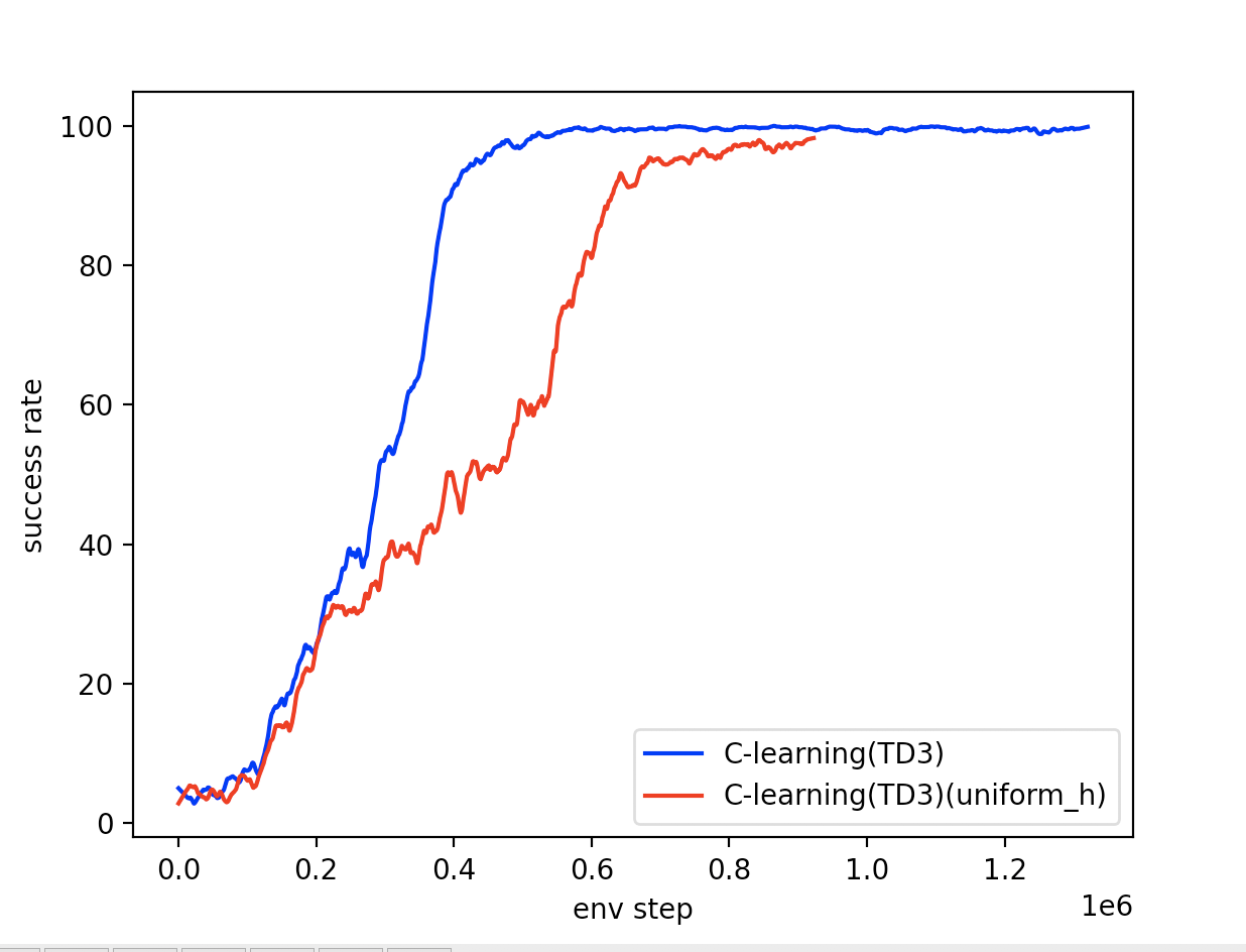
Reachability-guided sampling: When sampling a batch (line 1 of algorithm 1), for each i๐‘–i we first sample an episode from ๐’Ÿ๐’Ÿ\mathcal{D}, and then a transition (si,ai,siโ€ฒ)subscript๐‘ ๐‘–subscript๐‘Ž๐‘–subscriptsuperscript๐‘ โ€ฒ๐‘–(s_{i},a_{i},s^{\prime}_{i}) from that episode. We sample hisubscriptโ„Ž๐‘–h_{i} favoring smaller hโ„Žhโ€™s at the beginning of training. We achieve this by selecting hi=hsubscriptโ„Ž๐‘–โ„Žh_{i}=h with probability proportional to hโˆ’ฮบโ€‹nGโ€‹D/NGโ€‹Dsuperscriptโ„Ž๐œ…subscript๐‘›๐บ๐ทsubscript๐‘๐บ๐ทh^{-\kappa n_{GD}/N_{GD}}, where nGโ€‹Dsubscript๐‘›๐บ๐ทn_{GD} is the current episode number, NGโ€‹Dsubscript๐‘๐บ๐ทN_{GD} the total number of episodes, and ฮบ๐œ…\kappa is a hyperparameter. For deterministic environments, we follow HER (Andrychowicz etย al., 2017) and select gisubscript๐‘”๐‘–g_{i} uniformly at random from the states observed in the episode after sisubscript๐‘ ๐‘–s_{i}. For stochastic environments we use a slightly modified version, which addresses the bias incurred by HER (Matthias etย al., 2018) in the presence of stochasticity. All details are included in appendix G.

Extension to continuous action spaces: Note that constructing the targets yisubscript๐‘ฆ๐‘–y_{i} requires taking a maximum over the action space. While this is straightforward in discrete action spaces, it is not so for continuous actions. Lillicrap etย al. (2015) proposed DDPG, a method enabling deep Q๐‘„Q-learning in continuous action spaces. Similarly, Fujimoto etย al. (2018) proposed TD3, a method for further stabilizing Q๐‘„Q-learning. We note that C๐ถC-learning is compatible with the ideas underpinning both of these methods. We present a TD3 version of C๐ถC-learning in appendix E.

Parameter :ย Nexploresubscript๐‘exploreN_{\mathrm{explore}}: Number of random exploration episodes
Parameter :ย NGDsubscript๐‘GDN_{\mathrm{GD}}: Number of goal-directed episodes
Parameter :ย Ntrainsubscript๐‘trainN_{\mathrm{train}}: Number of batches to train on per goal-directed episode
Parameter :ย Ncopysubscript๐‘copyN_{\mathrm{copy}}: Number of batches between target network updates
Parameter :ย ฮฑ๐›ผ\alpha: Learning rate
1 ฮธโ†โ†๐œƒabsent\theta\leftarrow Initial weights for Cฮธโˆ—subscriptsuperscript๐ถ๐œƒC^{*}_{\theta}
ฮธโ€ฒโ†ฮธโ†superscript๐œƒโ€ฒ๐œƒ\theta^{\prime}\leftarrow\theta
ย  // Copy weights to target network
๐’Ÿโ†โ†๐’Ÿabsent\mathcal{D}\leftarrow[]
ย  // Initialize experience replay buffer
nbโ†0โ†subscript๐‘›b0n_{\mathrm{b}}\leftarrow 0
ย  // Counter for training batches
2 repeatย Nexploresubscript๐‘exploreN_{\mathrm{explore}}ย times
ย ย ย ย ย ย  โ„ฐโ†๐š๐šŽ๐šโ€‹_โ€‹๐š›๐š˜๐š•๐š•๐š˜๐šž๐šโ€‹(ฯ€random)โ†โ„ฐ๐š๐šŽ๐š_๐š›๐š˜๐š•๐š•๐š˜๐šž๐šsubscript๐œ‹random\mathcal{E}\leftarrow\mathtt{get\_rollout(}\pi_{\mathrm{random}}\mathtt{)}
ย ย ย ย ย ย ย  // Do a random rollout
ย ย ย ย ย ย  ๐’Ÿ.๐šŠ๐š™๐š™๐šŽ๐š—๐šโ€‹(โ„ฐ)formulae-sequence๐’Ÿ๐šŠ๐š™๐š™๐šŽ๐š—๐šโ„ฐ\mathcal{D}\mathtt{.append(}\mathcal{E}\mathtt{)}
ย ย ย ย ย ย ย  // Save the rollout to the buffer
3ย ย ย ย ย ย 
4
5repeatย NGDsubscript๐‘GDN_{\mathrm{GD}}ย times
ย ย ย ย ย ย  gโ†๐š๐š˜๐šŠ๐š•โ€‹_โ€‹๐šœ๐šŠ๐š–๐š™๐š•๐šŽโ€‹(nb)โ†๐‘”๐š๐š˜๐šŠ๐š•_๐šœ๐šŠ๐š–๐š™๐š•๐šŽsubscript๐‘›bg\leftarrow\mathtt{goal\_sample(}\mathcal{}n_{\mathrm{b}}\mathtt{)}
ย ย ย ย ย ย ย  // Sample a goal
ย ย ย ย ย ย  โ„ฐโ†๐š๐šŽ๐šโ€‹_โ€‹๐š›๐š˜๐š•๐š•๐š˜๐šž๐šโ€‹(ฯ€behavior)โ†โ„ฐ๐š๐šŽ๐š_๐š›๐š˜๐š•๐š•๐š˜๐šž๐šsubscript๐œ‹behavior\mathcal{E}\leftarrow\mathtt{get\_rollout(}\pi_{\mathrm{behavior}}\mathtt{)}
ย ย ย ย ย ย ย  // Try to reach the goal
ย ย ย ย ย ย  ๐’Ÿ.๐šŠ๐š™๐š™๐šŽ๐š—๐šโ€‹(โ„ฐ)formulae-sequence๐’Ÿ๐šŠ๐š™๐š™๐šŽ๐š—๐šโ„ฐ\mathcal{D}\mathtt{.append(}\mathcal{E}\mathtt{)}
ย ย ย ย ย ย ย  // Save the rollout
6ย ย ย ย ย ย  repeatย Ntrainsubscript๐‘trainN_{\mathrm{train}}ย times
7ย ย ย ย ย ย ย ย ย ย ย ย  ifย nbmodNcopy=0modulosubscript๐‘›bsubscript๐‘copy0n_{\mathrm{b}}\mod N_{\mathrm{copy}}=0ย then
ย ย ย ย ย ย ย ย ย ย ย ย ย ย ย ย ย ย  ฮธโ€ฒโ†ฮธโ†superscript๐œƒโ€ฒ๐œƒ\theta^{\prime}\leftarrow\theta
ย ย ย ย ย ย ย ย ย ย ย ย ย ย ย ย ย ย ย  // Copy weights periodically
8ย ย ย ย ย ย ย ย ย ย ย ย ย ย ย ย ย ย 
ย ย ย ย ย ย ย ย ย ย ย ย  โ„ฌ:={si,ai,siโ€ฒ,gi,hi}i=1|โ„ฌ|โ†๐šœ๐šŠ๐š–๐š™๐š•๐šŽโ€‹_โ€‹๐š‹๐šŠ๐š๐šŒ๐š‘โ€‹(๐’Ÿ)assignโ„ฌsuperscriptsubscriptsubscript๐‘ ๐‘–subscript๐‘Ž๐‘–subscriptsuperscript๐‘ โ€ฒ๐‘–subscript๐‘”๐‘–subscriptโ„Ž๐‘–๐‘–1โ„ฌโ†๐šœ๐šŠ๐š–๐š™๐š•๐šŽ_๐š‹๐šŠ๐š๐šŒ๐š‘๐’Ÿ\mathcal{B}:=\{s_{i},a_{i},s^{\prime}_{i},g_{i},h_{i}\}_{i=1}^{|\mathcal{B}|}\leftarrow\mathtt{sample\_batch(}\mathcal{D}\mathtt{)}
ย ย ย ย ย ย ย ย ย ย ย ย ย  // Sample a batch
ย ย ย ย ย ย ย ย ย ย ย ย  {yi}i=1|โ„ฌ|โ†๐š๐šŽ๐šโ€‹_โ€‹๐š๐šŠ๐š›๐š๐šŽ๐š๐šœโ€‹(โ„ฌ,ฮธโ€ฒ)โ†superscriptsubscriptsubscript๐‘ฆ๐‘–๐‘–1โ„ฌ๐š๐šŽ๐š_๐š๐šŠ๐š›๐š๐šŽ๐š๐šœโ„ฌsuperscript๐œƒโ€ฒ\left\{y_{i}\right\}_{i=1}^{\left|\mathcal{B}\right|}\leftarrow\mathtt{get\_targets(}\mathcal{B},\theta^{\prime}\mathtt{)}
ย ย ย ย ย ย ย ย ย ย ย ย ย  // Estimate RHS of equation 18
9ย ย ย ย ย ย ย ย ย ย ย ย  โ„’^โ†โˆ’1|โ„ฌ|โ€‹โˆ‘i=1|โ„ฌ|yiโ€‹logโกCฮธโˆ—โ€‹(si,ai,gi,hi)+(1โˆ’yi)โ€‹logโก(1โˆ’Cฮธโˆ—โ€‹(si,ai,gi,hi))โ†^โ„’1โ„ฌsuperscriptsubscript๐‘–1โ„ฌsubscript๐‘ฆ๐‘–subscriptsuperscript๐ถ๐œƒsubscript๐‘ ๐‘–subscript๐‘Ž๐‘–subscript๐‘”๐‘–subscriptโ„Ž๐‘–1subscript๐‘ฆ๐‘–1subscriptsuperscript๐ถ๐œƒsubscript๐‘ ๐‘–subscript๐‘Ž๐‘–subscript๐‘”๐‘–subscriptโ„Ž๐‘–\hat{\mathcal{L}}\leftarrow-\frac{1}{\left|\mathcal{B}\right|}\sum_{i=1}^{\left|\mathcal{B}\right|}y_{i}\log C^{*}_{\theta}(s_{i},a_{i},g_{i},h_{i})+(1-y_{i})\log\left(1-C^{*}_{\theta}(s_{i},a_{i},g_{i},h_{i})\right)
ย ย ย ย ย ย ย ย ย ย ย ย  ฮธโ†ฮธโˆ’ฮฑโ€‹โˆ‡ฮธโ„’^โ†๐œƒ๐œƒ๐›ผsubscriptโˆ‡๐œƒ^โ„’\theta\leftarrow\theta-\alpha\nabla_{\theta}\hat{\mathcal{L}}
ย ย ย ย ย ย ย ย ย ย ย ย ย  // Update weights
ย ย ย ย ย ย ย ย ย ย ย ย  nbโ†nb+1โ†subscript๐‘›bsubscript๐‘›b1n_{\mathrm{b}}\leftarrow n_{\mathrm{b}}+1
ย ย ย ย ย ย ย ย ย ย ย ย ย  // Trained one batch
10ย ย ย ย ย ย ย ย ย ย ย ย 
11ย ย ย ย ย ย 
12ย ย ย ย ย ย 
13
Algorithmย 1 Training C-learning Network

We finish this section by highlighting differences between C๐ถC-learning and related work. Ghosh etย al. (2019) proposed GCSL, a method for goal-reaching inspired by supervised learning. In their derivations, they also include a horizon hโ„Žh which their policies can depend on, but they drop this dependence in their experiments as they did not see a practical benefit by including hโ„Žh. We find the opposite for C๐ถC-learning. TDMs (Pong etย al., 2018) use horizon-aware policies and a similar recursion to ours. In practice they use a negative L1subscript๐ฟ1L_{1} distance reward, which significantly differs from our goal-reaching indicators. This is an important difference as TDMs operate under dense rewards, while we use sparse rewards, making the problem significantly more challenging. Additionally, distance between states in nonholonomic environments is very poorly described by L1subscript๐ฟ1L_{1} distance, resulting in TDMs being ill-suited for motion planning tasks. We also highlight that even if the reward in TDMs was swapped with our goal checking function G๐บG, the resulting objective would be much closer to the non-cumulative version of C๐ถC-learning presented in appendix C. TDMs recover policies from their horizon-aware Q๐‘„Q-function in a different manner to ours, not allowing a speed vs reliability trade-off. The recursion presented for TDMs is used by definition, whereas we have provided a mathematical derivation of the Bellman equation for C๐ถC-functions along with proofs of additional structure. As a result of the C๐ถC-function being a probability we use a different loss function (binary cross-entropy) which results in unbiased estimates of the objectiveโ€™s gradients. Finally, we point out that TDMs sample horizons uniformly at random, which differs from our specifically tailored replay buffer.

5 Experiments

5.1 Setup

Our experiments are designed to show that (i)๐‘–(i) C๐ถC-learning enables the speed vs reliability trade-off, (iโ€‹i)๐‘–๐‘–(ii) the Cโˆ—superscript๐ถC^{*} function recovered through C๐ถC-learning meaningfully matches reachability in nonholonomic environments, and (iโ€‹iโ€‹i)๐‘–๐‘–๐‘–(iii) C๐ถC-learning scales to complex and high-dimensional motion planning tasks, resulting in improved sample complexity and goal-reaching. We use success rate (percentage of trajectories which reach the goal) and path length (average, over trajectories and goals, number of steps needed to achieve the goal among successful trajectories) as metrics.

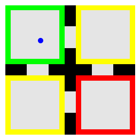
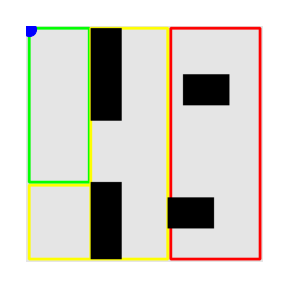
We compare C๐ถC-learning against GCSL (Ghosh etย al., 2019) (for discrete action states only) and deep Q๐‘„Q-learning with HER (Andrychowicz etย al., 2017) across several environments, which are depicted in Figure 3. All experimental details and hyperparameters are given in appendix G. We also provide ablations, and comparisons against TDMs and the alternative recursions from section 3.3 in appendix F. We evaluate C๐ถC-learning on the following domains:

  1. 1.

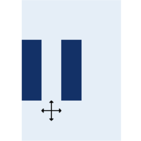
    Frozen lake is a 2D navigation environment where the agent must navigate without falling in the holes (dark blue). Both the state space (7ร—5757\times 5 grid, with two 3ร—1313\times 1 holes) and the action state are discrete. Falling in a hole terminates an episode. The agentโ€™s actions correspond to intended directions. The agent moves in the intended direction with probability 0.80.80.8, and in perpendicular directions with probabilities 0.10.10.1 each. Moving against the boundaries of the environment has no effect. We take ๐’ข=๐’ฎ๐’ข๐’ฎ\mathcal{G}=\mathcal{S} and Gโ€‹(s,g)=๐Ÿ™โ€‹(g=s)๐บ๐‘ ๐‘”1๐‘”๐‘ G(s,g)=\mathds{1}(g=s).

  2. 2.

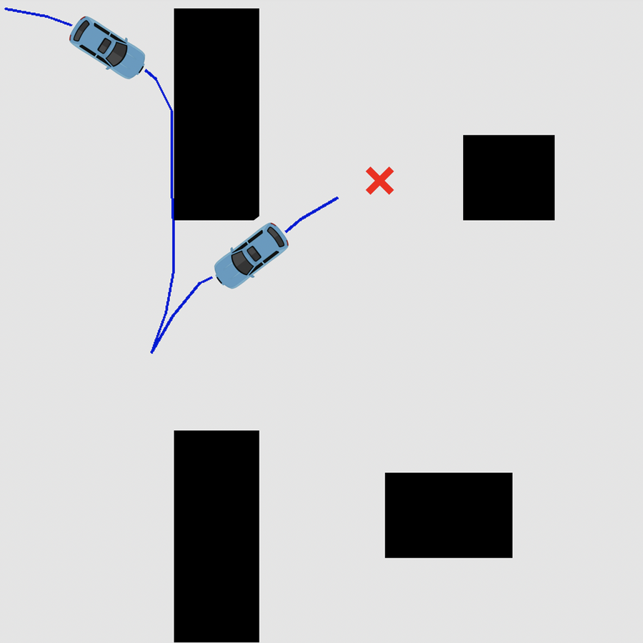
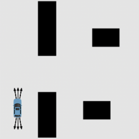
    Dubinsโ€™ car is a more challenging deterministic 2D navigation environment, where the agent drives a car which cannot turn by more than 10โˆ˜superscript1010^{\circ}. The states, with spatial coordinates in [0,15]2superscript0152[0,15]^{2}, are continuous and include the direction of the car. There are 7 actions: the 666 combinations of {leftโ€‹โ€‰10โˆ˜,straight,rightโ€‹โ€‰10โˆ˜}ร—{forwardโ€‹โ€‰1,reverseโ€‹โ€‰1}leftsuperscript10straightrightsuperscript10forward1reverse1\left\{\mathrm{left}\,10^{\circ},\,\mathrm{straight},\,\mathrm{right}\,10^{\circ}\right\}\times\left\{\mathrm{forward\,1},\,\mathrm{reverse\,1}\right\}, and the option to not move. As such, the set of reachable states is not simply a ball around the current state. The environment also has walls through which the car cannot drive. We take ๐’ข=[0,15]2๐’ขsuperscript0152\mathcal{G}=[0,15]^{2} and the goal is considered to be reached when the car is within an Lโˆžsubscript๐ฟL_{\infty} distance of 0.50.50.5 from the goal, regardless of its orientation.

  3. 3.

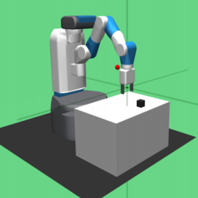
    FetchPickAndPlace-v1 (Brockman etย al., 2016) is a complex, higher-dimensional environment in which a robotic arm needs to pick up a block and move it to the goal location. Goals are defined by their 3-dimensional coordinates. The state space is 252525-dimensional, and the action space is continuous and 444-dimensional.

  4. 4.

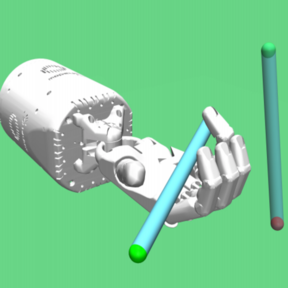
    HandManipulatePenFull-v0 (Brockman etย al., 2016) is a realistic environment known the be a difficult goal-reaching problem, where deep Q-learning with HER shows very limited success (Plappert etย al., 2018). The environment has a continuous action space of dimension 202020, a 636363-dimensional state space, and 777-dimensional goals. Note that we are considering the more challenging version of the environment where both target location and orientation are chosen randomly.
Refer to caption
Refer to caption
Refer to caption
Refer to caption
Figure 3: Experimental environments, from left to right: frozen lake, Dubinsโ€™ car, FetchPickAndPlace-v1 and HandManipulatePenFull-v0. Arrows represent actions (only their direction should be considered, their magnitude is not representative of the distance travelled by an agent taking an action). See text for description.

5.2 Results

Speed vs reliability trade-off: We use frozen lake to illustrate this trade-off. At test time, we set the starting state and goal as shown in Figure 4(a). Notice that, given enough time, an agent can reach the goal with near certainty by going around the holes on the right side of the lake. However, if the agent is time-constrained, the optimal policy must accept the risk of falling in a hole. We see that C๐ถC-learning does indeed learn both the risky and safe policies. Other methods, as previously explained, can only learn one. To avoid re-plotting the environment for every horizon, we have plotted arrows in Figure 4(a) corresponding to argโ€‹maxaโกฯ€โˆ—โ€‹(a|s0,g,h)subscriptargmax๐‘Žsuperscript๐œ‹conditional๐‘Žsubscript๐‘ 0๐‘”โ„Ž\operatorname*{arg\,max}_{a}\pi^{*}(a|s_{0},g,h), argโ€‹maxaโกฯ€โˆ—โ€‹(a|s1,g,hโˆ’1)subscriptargmax๐‘Žsuperscript๐œ‹conditional๐‘Žsubscript๐‘ 1๐‘”โ„Ž1\operatorname*{arg\,max}_{a}\pi^{*}(a|s_{1},g,h-1), argโ€‹maxaโกฯ€โˆ—โ€‹(a|s2,g,hโˆ’2)subscriptargmax๐‘Žsuperscript๐œ‹conditional๐‘Žsubscript๐‘ 2๐‘”โ„Ž2\operatorname*{arg\,max}_{a}\pi^{*}(a|s_{2},g,h-2) and so on, where st+1subscript๐‘ ๐‘ก1s_{t+1} is obtained from the previous state and action while ignoring the randomness in the environment (i.e. st+1=argโ€‹maxsโกpโ€‹(s|st,at)subscript๐‘ ๐‘ก1subscriptargmax๐‘ ๐‘conditional๐‘ subscript๐‘ ๐‘กsubscript๐‘Ž๐‘กs_{t+1}=\operatorname*{arg\,max}_{s}p(s|s_{t},a_{t})). In other words, we are plotting the most likely trajectory of the agent. When given the minimal amount of time to reach the goal (h=6โ„Ž6h=6), the CAE agent learns correctly to accept the risk of falling in a hole by taking the direct path. When given four times as long (h=24โ„Ž24h=24), the agent takes a safer path by going around the hole. Notice that the agent makes a single mistake at the upper right corner, which is quickly corrected when the value of hโ„Žh is decreased. On the other hand, we can see on the bottom panel that both GCSL and HER recover a single policy, thus not enabling the speed vs reliability trade-off. Surprisingly, GCSL learns to take the high-risk path, despite Ghosh etย al. (2019)โ€™s intention to incentivize paths that are guaranteed to reach the goal.

Reachability learning: To demonstrate that we are adequately learning reachability, we removed the walls from Dubinsโ€™ car and further restricted the turning angles to 5โˆ˜superscript55^{\circ}, thus making the dumbbell shape of the true reachable region more extreme. In Figure 4(b), we show that our learned Cโˆ—superscript๐ถC^{*} function correctly learns which goals are reachable from which states for different time horizons in Dubinsโ€™ car: not only is the learned Cโˆ—superscript๐ถC^{*} function increasing in hโ„Žh, but the shapes are as expected. None of the competing alternatives recover this information in any way, and thus comparisons are not available. As previously mentioned, the optimal Cโˆ—superscript๐ถC^{*}-function in this task is not trivial. Reachability is defined by the โ€œgeodesicsโ€ in ๐’ฎ=[0,15]2ร—S1๐’ฎsuperscript0152superscript๐‘†1\mathcal{S}=\left[0,15\right]^{2}\times S^{1} that are constrained by the finite turning radius, and thus follow a more intricate structure than a ball in โ„2superscriptโ„2\mathbb{R}^{2}.

Refer to caption
Refer to caption
(a)
Refer to caption
Refer to caption
Refer to caption
(b)
Refer to caption
Refer to caption
Refer to caption
(c)
Refer to caption
Refer to caption
Refer to caption
(d)
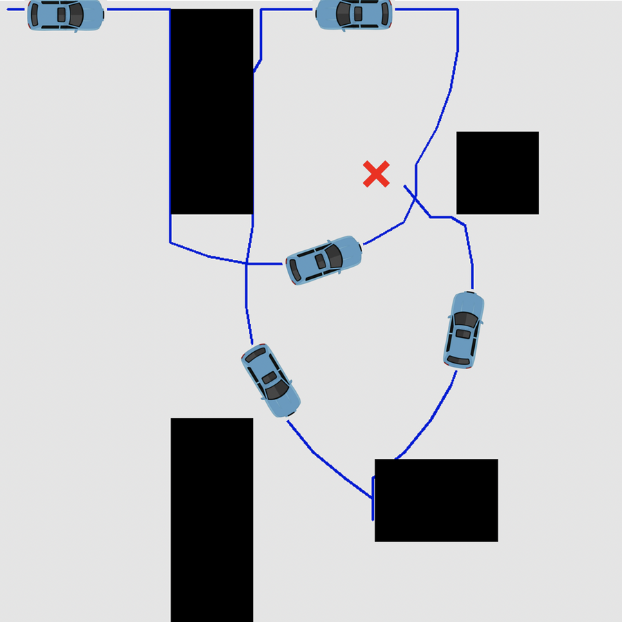
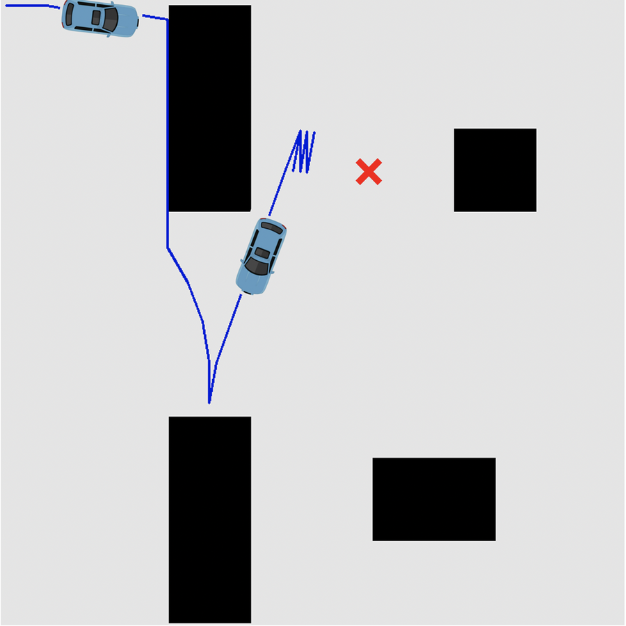
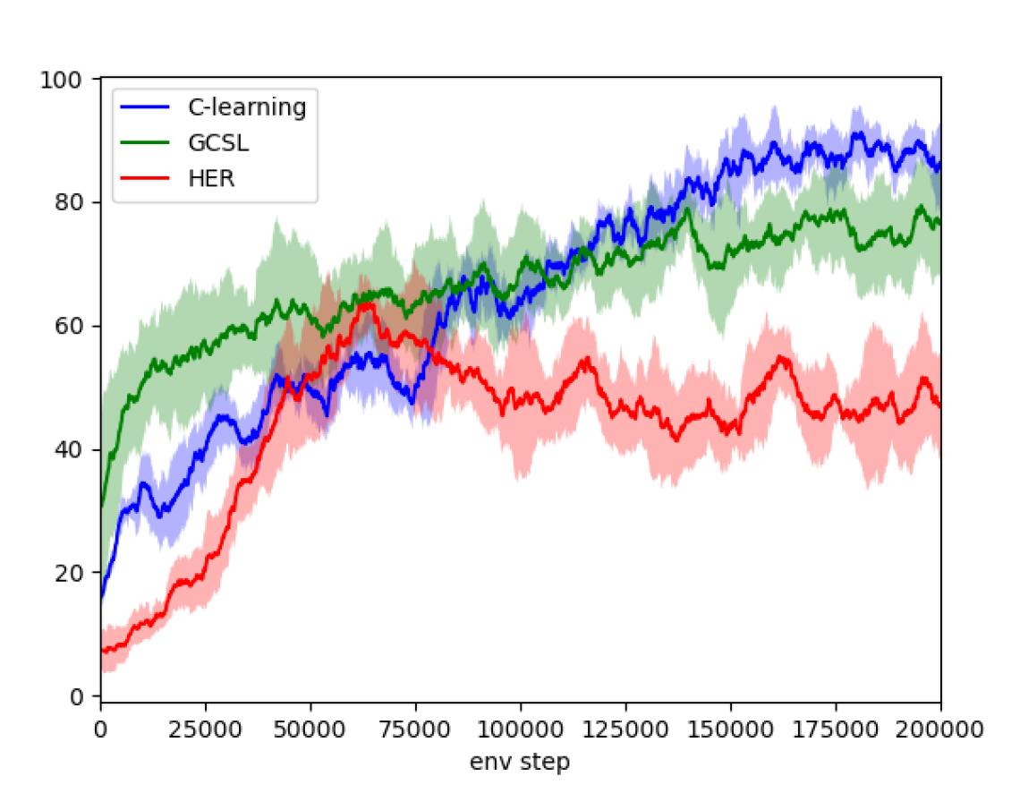
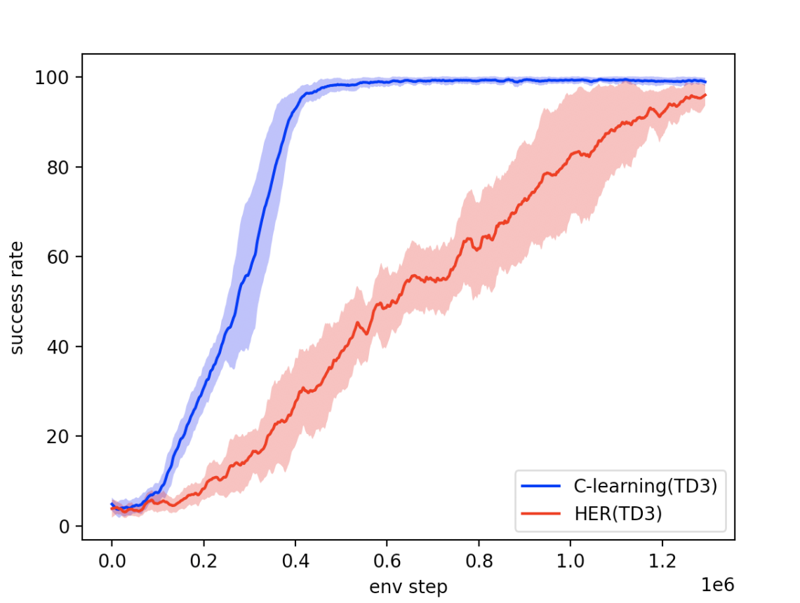
Figure 4: (a)๐‘Ž(a) Multimodal policies recovered by C๐ถC-learning in frozen lake for different values of hโ„Žh for reaching (G)๐บ(G) from (S)๐‘†(S) (top); unimodal policies recovered by GCSL and HER (bottom). (b)๐‘(b) Heatmaps over the goal space of maxaโกCโˆ—โ€‹(s,a,g,h)subscript๐‘Žsuperscript๐ถ๐‘ ๐‘Ž๐‘”โ„Ž\max_{a}C^{*}(s,a,g,h) with a fixed s๐‘ s and hโ„Žh for Dubinsโ€™ car, with h=7โ„Ž7h=7 (top), h=15โ„Ž15h=15 (middle) and h=25โ„Ž25h=25 (bottom). (c)๐‘(c) Trajectories learned by C๐ถC-learning (top), GCSL (middle) and HER (bottom) for Dubinsโ€™ car. (d)๐‘‘(d) Success rate throughout the training for Dubinsโ€™ car (top), FetchPickAndPlace-v1 (middle) and HandManipulatePenFull-v0 (bottom) for C๐ถC-learning (blue), HER (red) and GCSL (green).

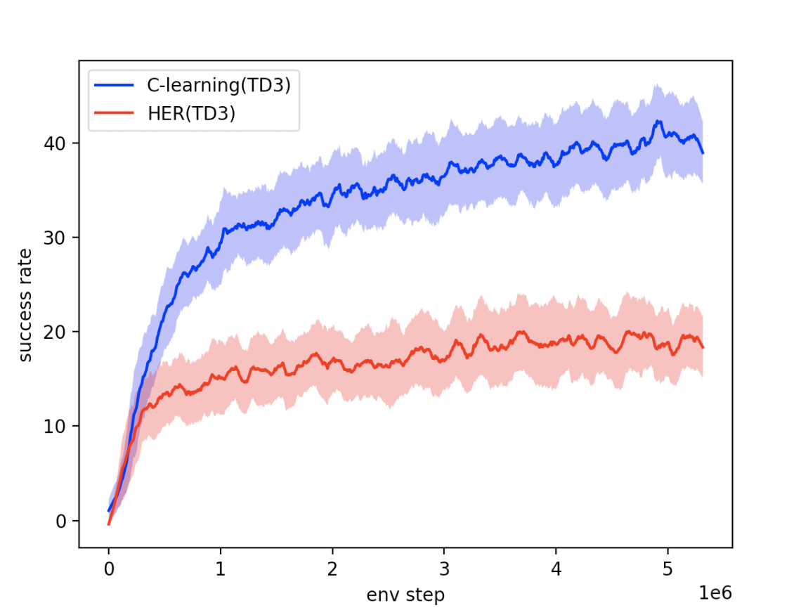
Motion planning and goal-reaching: For a qualitative comparison of performance for goal-reaching, Figure 4(c) shows trajectories for C๐ถC-learning and competing alternatives for Dubinsโ€™ car. We can see that C๐ถC-learning finds the optimal route, which is a combination of forward and backward movement, while other methods find inefficient paths. We also evaluated our method on challenging goal reaching environments, and observed that C๐ถC-learning achieves state-of-the-art results both in sample complexity and success rate. Figure 4(d) shows that C๐ถC-learning is able to learn considerably faster in the FetchPickAndPlace-v1 environment. More importantly, C๐ถC-learning achieves an absolute 20%percent2020\% improvement in its success rate over the current state-of-the-art algorithm HER (TD3) in the HandManipulatePenFull-v0 environment. Quantitative results are shown in Table 1. On Dubinsโ€™ car, we also note that C๐ถC-learning ends up with a smaller final Lโˆžsubscript๐ฟL_{\infty} distance to the goal: 0.93ยฑ0.15plus-or-minus0.930.15\mathbf{0.93\pm 0.15} vs.ย 1.28ยฑ0.51plus-or-minus1.280.511.28\pm 0.51 for GCSL.

Table 1: Comparison of C๐ถC-Learning against relevant benchmarks in three environments, averaged across five random seeds. Runs in bold are either the best on the given metric in that environment, or have a mean score within the error bars of the best.
ENVIRONMENT METHOD SUCCESS RATE PATH LENGTH
Dubinsโ€™ Car CAE 86.15%ยฑ2.44%plus-or-minuspercent86.15percent2.44\mathbf{86.15\%\pm 2.44}\% 16.45ยฑ0.99plus-or-minus16.450.99\mathbf{16.45\pm 0.99}
GCSL 79.69%ยฑ6.35%plus-or-minuspercent79.69percent6.3579.69\%\pm 6.35\% 32.64ยฑ6.16plus-or-minus32.646.1632.64\pm 6.16
HER 51.25%ยฑ6.48%plus-or-minuspercent51.25percent6.4851.25\%\pm 6.48\% 20.13ยฑ1.66plus-or-minus20.131.6620.13\pm 1.66
FetchPickAndPlace-v1 CAE (TD3) 99.34%ยฑ0.27%plus-or-minuspercent99.34percent0.27\mathbf{99.34\%\pm 0.27\%} 8.53ยฑ0.09plus-or-minus8.530.09\mathbf{8.53\pm 0.09}
HER (TD3) 98.25%ยฑ2.51%plus-or-minuspercent98.25percent2.5198.25\%\pm 2.51\% 8.86ยฑ0.14plus-or-minus8.860.148.86\pm 0.14
HandManipulatePenFull-v0 CAE (TD3) 39.83%ยฑ1.64%plus-or-minuspercent39.83percent1.64\mathbf{39.83\%\pm 1.64\%} 7.68ยฑ0.90plus-or-minus7.680.90\mathbf{7.68\pm 0.90}
HER (TD3) 21.99%ยฑ2.46%plus-or-minuspercent21.99percent2.4621.99\%\pm 2.46\% 15.03ยฑ0.71plus-or-minus15.030.7115.03\pm 0.71

6 Discussion

We have shown that C๐ถC-learning enables simultaneous learning of how to reach goals quickly and how to reach them safely, which current methods cannot do. We point out that reaching the goal safely in our setting means doing so at test time, and is different to what is usually considered in the safety literature where safe exploration is desired (Chow etย al., 2018; Bharadhwaj etย al., 2020b). Additionally, learning Cโˆ—superscript๐ถC^{*} effectively learns reachability within an environment, and could thus naturally lends itself to incorporation into other frameworks, for example, in goal setting for hierarchical RL tasks (Nachum etย al., 2018) where intermediate, reachable goals need to be selected sequentially. We believe further investigations on using C๐ถC-functions on safety-critical environments requiring adaptation (Peng etย al., 2018; Zhang etย al., 2020), or for hierarchical RL, are promising directions for further research.

We have also argued that C๐ถC-functions are more tolerant of errors during learning than Q๐‘„Q-functions which increases sample efficiency. This is verified empirically in that C๐ถC-learning is able to solve goal-reaching tasks earlier on in training than Q๐‘„Q-learning.

We finish by noticing a parallel between C๐ถC-learning and the options framework (Sutton etย al., 1999; Bacon etย al., 2017), which introduces temporal abstraction and allows agents to not always follow the same policy when at a given state s๐‘ s. However, our work does not fit within this framework, as options evolve stochastically and new options are selected according only to the current state, while horizons evolve deterministically and depend on the previous horizon only, not the state. Additionally, and unlike C๐ถC-learning, nothing encourages different options to learn safe or quick policies, and there is no reachability information contained in options.

7 Conclusions

In this paper we introduced C๐ถC-learning, a Q๐‘„Q-learning-inspired method for goal-reaching. Unlike previous approaches, we propose the use of horizon-aware policies, and show that not only can these policies be tuned to reach the goal faster or more reliably, but they also outperform horizon-unaware approaches for goal-reaching on complex motion planning tasks. We hope our method will inspire further research into horizon-aware policies and their benefits.

References

  • Andrychowicz etย al. (2017) Marcin Andrychowicz, Filip Wolski, Alex Ray, Jonas Schneider, Rachel Fong, Peter Welinder, Bob McGrew, Josh Tobin, Pieter Abbeel, and Wojciech Zaremba. Hindsight experience replay. In Advances in neural information processing systems, pp.ย 5048โ€“5058, 2017.
  • Bacon etย al. (2017) Pierre-Luc Bacon, Jean Harb, and Doina Precup. The option-critic architecture. In Thirty-First AAAI Conference on Artificial Intelligence, 2017.
  • Bellemare etย al. (2017) Marcย G Bellemare, Will Dabney, and Rรฉmi Munos. A distributional perspective on reinforcement learning. arXiv preprint arXiv:1707.06887, 2017.
  • Bharadhwaj etย al. (2020a) Homanga Bharadhwaj, Animesh Garg, and Florian Shkurti. Leaf: Latent exploration along the frontier. arXiv preprint arXiv:2005.10934, 2020a.
  • Bharadhwaj etย al. (2020b) Homanga Bharadhwaj, Aviral Kumar, Nicholas Rhinehart, Sergey Levine, Florian Shkurti, and Animesh Garg. Conservative safety critics for exploration. arXiv preprint arXiv:2010.14497, 2020b.
  • Brockman etย al. (2016) Greg Brockman, Vicki Cheung, Ludwig Pettersson, Jonas Schneider, John Schulman, Jie Tang, and Wojciech Zaremba. Openai gym, 2016.
  • Chow etย al. (2018) Yinlam Chow, Ofir Nachum, Edgar Duenez-Guzman, and Mohammad Ghavamzadeh. A lyapunov-based approach to safe reinforcement learning. In Advances in neural information processing systems, pp.ย 8092โ€“8101, 2018.
  • Fujimoto etย al. (2018) Scott Fujimoto, Herke Vanย Hoof, and David Meger. Addressing function approximation error in actor-critic methods. arXiv preprint arXiv:1802.09477, 2018.
  • Ghosh etย al. (2018) Dibya Ghosh, Abhishek Gupta, and Sergey Levine. Learning actionable representations with goal-conditioned policies. arXiv preprint arXiv:1811.07819, 2018.
  • Ghosh etย al. (2019) Dibya Ghosh, Abhishek Gupta, Ashwin Reddy, Justin Fu, Coline Devin, Benjamin Eysenbach, and Sergey Levine. Learning to Reach Goals via Iterated Supervised Learning. arXiv e-prints, art. arXiv:1912.06088, December 2019.
  • Haarnoja etย al. (2018) Tuomas Haarnoja, Aurick Zhou, Pieter Abbeel, and Sergey Levine. Soft actor-critic: Off-policy maximum entropy deep reinforcement learning with a stochastic actor. arXiv preprint arXiv:1801.01290, 2018.
  • Kaelbling (1993) Leslieย Pack Kaelbling. Learning to achieve goals. In IJCAI, pp.ย  1094โ€“1099. Citeseer, 1993.
  • Lillicrap etย al. (2015) Timothyย P Lillicrap, Jonathanย J Hunt, Alexander Pritzel, Nicolas Heess, Tom Erez, Yuval Tassa, David Silver, and Daan Wierstra. Continuous control with deep reinforcement learning. arXiv preprint arXiv:1509.02971, 2015.
  • Matthias etย al. (2018) Plappert Matthias, Marcin Andrychowicz, Alex Ray, Bob McGrew, Bowen Baker, Glenn Powell, Jonas Schneider, Josh Tobin, Maciek Chociej, Peter Welinder, Vikash Kumar, and Wojciech Zaremba. Multi-goal reinforcement learning: Challenging robotics environments and request for research. arXiv preprint arXiv:1802.09464, 2018.
  • Mnih etย al. (2015) Volodymyr Mnih, Koray Kavukcuoglu, David Silver, Andreiย A Rusu, Joel Veness, Marcย G Bellemare, Alex Graves, Martin Riedmiller, Andreasย K Fidjeland, Georg Ostrovski, etย al. Human-level control through deep reinforcement learning. nature, 518(7540):529โ€“533, 2015.
  • Nachum etย al. (2018) Ofir Nachum, Shixiangย Shane Gu, Honglak Lee, and Sergey Levine. Data-efficient hierarchical reinforcement learning. In Advances in Neural Information Processing Systems, pp.ย 3303โ€“3313, 2018.
  • Peng etย al. (2018) Xueย Bin Peng, Marcin Andrychowicz, Wojciech Zaremba, and Pieter Abbeel. Sim-to-real transfer of robotic control with dynamics randomization. In 2018 IEEE international conference on robotics and automation (ICRA), pp.ย  1โ€“8. IEEE, 2018.
  • Plappert etย al. (2018) Matthias Plappert, Marcin Andrychowicz, Alex Ray, Bob McGrew, Bowen Baker, Glenn Powell, Jonas Schneider, Josh Tobin, Maciek Chociej, Peter Welinder, etย al. Multi-goal reinforcement learning: Challenging robotics environments and request for research. arXiv preprint arXiv:1802.09464, 2018.
  • Pong etย al. (2018) Vitchyr Pong, Shixiang Gu, Murtaza Dalal, and Sergey Levine. Temporal difference models: Model-free deep rl for model-based control. arXiv preprint arXiv:1802.09081, 2018.
  • Pong etย al. (2019) Vitchyrย H Pong, Murtaza Dalal, Steven Lin, Ashvin Nair, Shikhar Bahl, and Sergey Levine. Skew-fit: State-covering self-supervised reinforcement learning. arXiv preprint arXiv:1903.03698, 2019.
  • Qureshi etย al. (2020) Ahmed Qureshi, Yinglong Miao, Anthony Simeonov, and Michael Yip. Motion planning networks: Bridging the gap between learning-based and classical motion planners. arXiv preprint arXiv:1907.06013, 2020.
  • Savinov etย al. (2018) Nikolay Savinov, Anton Raichuk, Raphaรซl Marinier, Damien Vincent, Marc Pollefeys, Timothy Lillicrap, and Sylvain Gelly. Episodic curiosity through reachability. arXiv preprint arXiv:1810.02274, 2018.
  • Schaul etย al. (2015) Tom Schaul, Daniel Horgan, Karol Gregor, and David Silver. Universal value function approximators. In International conference on machine learning, pp.ย 1312โ€“1320, 2015.
  • Sill (1998) Joseph Sill. Monotonic networks. In Advances in neural information processing systems, pp.ย 661โ€“667, 1998.
  • Sutton etย al. (1998) Richardย S Sutton, Andrewย G Barto, etย al. Introduction to reinforcement learning, volume 135. MIT press Cambridge, 1998.
  • Sutton etย al. (1999) Richardย S Sutton, Doina Precup, and Satinder Singh. Between mdps and semi-mdps: A framework for temporal abstraction in reinforcement learning. Artificial intelligence, 112(1-2):181โ€“211, 1999.
  • Vanย Hasselt etย al. (2015) Hado Vanย Hasselt, Arthur Guez, and David Silver. Deep reinforcement learning with double q-learning. arXiv preprint arXiv:1509.06461, 2015.
  • Venkattaramanujam etย al. (2019) Srinivas Venkattaramanujam, Eric Crawford, Thang Doan, and Doina Precup. Self-supervised learning of distance functions for goal-conditioned reinforcement learning. arXiv preprint arXiv:1907.02998, 2019.
  • Watkins & Dayan (1992) Christopherย JCH Watkins and Peter Dayan. Q-learning. Machine learning, 8(3-4):279โ€“292, 1992.
  • Wehenkel & Louppe (2019) Antoine Wehenkel and Gilles Louppe. Unconstrained monotonic neural networks. In Advances in Neural Information Processing Systems, pp.ย 1545โ€“1555, 2019.
  • Zhang etย al. (2020) Jesse Zhang, Brian Cheung, Chelsea Finn, Sergey Levine, and Dinesh Jayaraman. Cautious adaptation for reinforcement learning in safety-critical settings. arXiv preprint arXiv:2008.06622, 2020.

Appendix A Proofs of propositions

Proposition 1: Cฯ€superscript๐ถ๐œ‹C^{\pi} can be framed as a Q๐‘„Q-function within the MDP formalism, and if ฯ€โˆ—superscript๐œ‹\pi^{*} is optimal in the sense that Cฯ€โˆ—โ€‹(s,a,g,h)โ‰ฅCฯ€โ€‹(s,a,g,h)superscript๐ถsuperscript๐œ‹๐‘ ๐‘Ž๐‘”โ„Žsuperscript๐ถ๐œ‹๐‘ ๐‘Ž๐‘”โ„ŽC^{\pi^{*}}(s,a,g,h)\geq C^{\pi}(s,a,g,h) for every ฯ€๐œ‹\pi and (s,a,g,h)โˆˆ๐’ฎร—๐’œร—๐’ขร—โ„•๐‘ ๐‘Ž๐‘”โ„Ž๐’ฎ๐’œ๐’ขโ„•(s,a,g,h)\in\mathcal{S}\times\mathcal{A}\times\mathcal{G}\times\mathbb{N}, then Cฯ€โˆ—superscript๐ถsuperscript๐œ‹C^{\pi^{*}} matches the optimal C๐ถC-function, Cโˆ—superscript๐ถC^{*}, which obeys the following equation:

Cโˆ—โ€‹(s,a,g,h)={๐”ผsโ€ฒโˆผp(โ‹…|s,a)โ€‹[maxaโ€ฒโˆˆ๐’œโกCโˆ—โ€‹(sโ€ฒ,aโ€ฒ,g,hโˆ’1)]โ€‹ย ifย โ€‹Gโ€‹(s,g)=0โ€‹ย andย โ€‹hโ‰ฅ1,Gโ€‹(s,g)ย otherwise.C^{*}(s,a,g,h)=\begin{cases}\mathbb{E}_{s^{\prime}\sim p(\cdot|s,a)}\left[\displaystyle\max_{a^{\prime}\in\mathcal{A}}C^{*}(s^{\prime},a^{\prime},g,h-1)\right]\text{ if }G(s,g)=0\text{ and }h\geq 1,\\ G(s,g)\hskip 127.0pt\text{ otherwise}.\end{cases}

Proof: First, we frame C๐ถC-functions within the MDP formalism. Consider a state space given by ๐’ฎโ€ฒ=๐’ฎร—๐’ขร—โ„•superscript๐’ฎโ€ฒ๐’ฎ๐’ขโ„•\mathcal{S}^{\prime}=\mathcal{S}\times\mathcal{G}\times\mathbb{N}, where states corresponding to reached goals (i.e. Gโ€‹(s,g)=1๐บ๐‘ ๐‘”1G(s,g)=1) or with last coordinate equal to 00 (i.e. h=0โ„Ž0h=0) are considered terminal. The dynamics in this environment are given by:

pโ€‹(st+1,gt+1,ht+1|st,gt,ht,at)=pโ€‹(st+1|st,at)โ€‹๐Ÿ™โ€‹(gt+1=gt)โ€‹๐Ÿ™โ€‹(ht+1=htโˆ’1).๐‘subscript๐‘ ๐‘ก1subscript๐‘”๐‘ก1conditionalsubscriptโ„Ž๐‘ก1subscript๐‘ ๐‘กsubscript๐‘”๐‘กsubscriptโ„Ž๐‘กsubscript๐‘Ž๐‘ก๐‘conditionalsubscript๐‘ ๐‘ก1subscript๐‘ ๐‘กsubscript๐‘Ž๐‘ก1subscript๐‘”๐‘ก1subscript๐‘”๐‘ก1subscriptโ„Ž๐‘ก1subscriptโ„Ž๐‘ก1p(s_{t+1},g_{t+1},h_{t+1}|s_{t},g_{t},h_{t},a_{t})=p(s_{t+1}|s_{t},a_{t})\mathds{1}(g_{t+1}=g_{t})\mathds{1}(h_{t+1}=h_{t}-1)\,. (7)

That is, states evolve according to the original dynamics, while goals remain unchanged and horizons decrease by one at every step. The initial distribution is given by:

pโ€‹(s0,g0,h0)=pโ€‹(s0)โ€‹pโ€‹(g0,h0|s0),๐‘subscript๐‘ 0subscript๐‘”0subscriptโ„Ž0๐‘subscript๐‘ 0๐‘subscript๐‘”0conditionalsubscriptโ„Ž0subscript๐‘ 0p(s_{0},g_{0},h_{0})=p(s_{0})p(g_{0},h_{0}|s_{0})\,, (8)

where pโ€‹(s0)๐‘subscript๐‘ 0p(s_{0}) corresponds to the original starting distribution and pโ€‹(g0,h0|s0)๐‘subscript๐‘”0conditionalsubscriptโ„Ž0subscript๐‘ 0p(g_{0},h_{0}|s_{0}) needs to be specified beforehand. Together, the initial distribution and the dynamics, along with a policy ฯ€โ€‹(a|s,g,h)๐œ‹conditional๐‘Ž๐‘ ๐‘”โ„Ž\pi(a|s,g,h) properly define a distribution over trajectories, and again, we use โ„™ฯ€(โ‹…|โ‹…,g,h)\mathbb{P}_{\pi(\cdot|\cdot,g,h)} to denote probabilities with respect to this distribution. The reward function r:๐’ฎโ€ฒร—๐’œโ†’โ„:๐‘Ÿโ†’superscript๐’ฎโ€ฒ๐’œโ„r:\mathcal{S}^{\prime}\times\mathcal{A}\rightarrow\mathbb{R} is given by:

rโ€‹(s,a,g,h)=Gโ€‹(s,g).๐‘Ÿ๐‘ ๐‘Ž๐‘”โ„Ž๐บ๐‘ ๐‘”r(s,a,g,h)=G(s,g)\,. (9)

By taking the discount factor to be 111, and since we take states for which Gโ€‹(s,g)=1๐บ๐‘ ๐‘”1G(s,g)=1 to be terminal, the return (sum of rewards) over a trajectory (s0,s1,โ€ฆ)subscript๐‘ 0subscript๐‘ 1โ€ฆ(s_{0},s_{1},\dots) with h0=hsubscriptโ„Ž0โ„Žh_{0}=h is given by:

maxt=0,โ€ฆ,hโกGโ€‹(st,g).subscript๐‘ก0โ€ฆโ„Ž๐บsubscript๐‘ ๐‘ก๐‘”\displaystyle\max_{t=0,\dots,h}G(s_{t},g)\,. (10)

For notational simplicity we take Gโ€‹(st,g)=0๐บsubscript๐‘ ๐‘ก๐‘”0G(s_{t},g)=0 whenever t๐‘กt is greater than the length of the trajectory to properly account for terminal states. Since the return is binary, its expectation matches its probability of being equal to 111, so that indeed, the Q๐‘„Q-functions in this MDP correspond to Cฯ€superscript๐ถ๐œ‹C^{\pi}:

Cฯ€(s,a,g,h)=โ„™ฯ€(โ‹…|โ‹…,g,h)(maxt=0,โ€ฆ,hG(St,g)=1|s0=s,a0=a).C^{\pi}(s,a,g,h)=\mathbb{P}_{\pi(\cdot|\cdot,g,h)}\left(\displaystyle\max_{t=0,\dots,h}G(S_{t},g)=1\middle|s_{0}=s,a_{0}=a\right).

Now, we derive the Bellman equation for our C๐ถC-functions. Trivially:

Cฯ€โ€‹(s,a,g,h)=Gโ€‹(s,g),superscript๐ถ๐œ‹๐‘ ๐‘Ž๐‘”โ„Ž๐บ๐‘ ๐‘”C^{\pi}(s,a,g,h)=G(s,g), (11)

whenever Gโ€‹(s,g)=1๐บ๐‘ ๐‘”1G(s,g)=1 or h=0โ„Ž0h=0. For the rest of the derivation, we assume that Gโ€‹(s,g)=0๐บ๐‘ ๐‘”0G(s,g)=0 and hโ‰ฅ1โ„Ž1h\geq 1. We note that the probability of reaching g๐‘”g from s๐‘ s in at most hโ„Žh steps is given by the probability of reaching it in exactly one step, plus the probability of not reaching it in the first step and reaching it in at most hโˆ’1โ„Ž1h-1 steps thereafter. Formally:

Cฯ€โ€‹(s,a,g,h)superscript๐ถ๐œ‹๐‘ ๐‘Ž๐‘”โ„Ž\displaystyle C^{\pi}(s,a,g,h) (12)
=Cฯ€โ€‹(s,a,g,1)+๐”ผsโ€ฒโˆผp(โ‹…|s,a)โ€‹[(1โˆ’Gโ€‹(sโ€ฒ,g))โ€‹๐”ผaโ€ฒโˆผฯ€(โ‹…|sโ€ฒ,g,hโˆ’1)โ€‹[Cฯ€โ€‹(sโ€ฒ,aโ€ฒ,g,hโˆ’1)]]\displaystyle=C^{\pi}(s,a,g,1)+\mathbb{E}_{s^{\prime}\sim p(\cdot|s,a)}\left[(1-G(s^{\prime},g))\mathbb{E}_{a^{\prime}\sim\pi(\cdot|s^{\prime},g,h-1)}\left[C^{\pi}(s^{\prime},a^{\prime},g,h-1)\right]\right]
=๐”ผsโ€ฒโˆผp(โ‹…|s,a)โ€‹[Gโ€‹(sโ€ฒ,g)]+๐”ผsโ€ฒโˆผp(โ‹…|s,a)โ€‹[(1โˆ’Gโ€‹(sโ€ฒ,g))โ€‹๐”ผaโ€ฒโˆผฯ€(โ‹…|sโ€ฒ,g,hโˆ’1)โ€‹[Cฯ€โ€‹(sโ€ฒ,aโ€ฒ,g,hโˆ’1)]]\displaystyle=\mathbb{E}_{s^{\prime}\sim p(\cdot|s,a)}[G(s^{\prime},g)]+\mathbb{E}_{s^{\prime}\sim p(\cdot|s,a)}\left[(1-G(s^{\prime},g))\mathbb{E}_{a^{\prime}\sim\pi(\cdot|s^{\prime},g,h-1)}\left[C^{\pi}(s^{\prime},a^{\prime},g,h-1)\right]\right]
=๐”ผsโ€ฒโˆผp(โ‹…|s,a)โ€‹[๐”ผaโ€ฒโˆผฯ€(โ‹…|sโ€ฒ,g,hโˆ’1)โ€‹[Cฯ€โ€‹(sโ€ฒ,aโ€ฒ,g,hโˆ’1)]],\displaystyle=\mathbb{E}_{s^{\prime}\sim p(\cdot|s,a)}\left[\mathbb{E}_{a^{\prime}\sim\pi(\cdot|s^{\prime},g,h-1)}\left[C^{\pi}(s^{\prime},a^{\prime},g,h-1)\right]\right],

where the last equality follows from the fact that Cฯ€โ€‹(sโ€ฒ,aโ€ฒ,g,hโˆ’1)=1superscript๐ถ๐œ‹superscript๐‘ โ€ฒsuperscript๐‘Žโ€ฒ๐‘”โ„Ž11C^{\pi}(s^{\prime},a^{\prime},g,h-1)=1 whenever Gโ€‹(sโ€ฒ,g)=1๐บsuperscript๐‘ โ€ฒ๐‘”1G(s^{\prime},g)=1. Putting everything together, we obtain the Bellman equation for Cฯ€superscript๐ถ๐œ‹C^{\pi}:

Cฯ€โ€‹(s,a,g,h)={๐”ผsโ€ฒโˆผp(โ‹…|s,a)โ€‹[๐”ผaโ€ฒโˆผฯ€(โ‹…|sโ€ฒ,g,hโˆ’1)โ€‹[Cฯ€โ€‹(sโ€ฒ,aโ€ฒ,g,hโˆ’1)]]โ€‹ย ifย โ€‹Gโ€‹(s,g)=0โ€‹ย andย โ€‹hโ‰ฅ1,Gโ€‹(s,g)ย otherwise.C^{\pi}(s,a,g,h)=\begin{cases}\mathbb{E}_{s^{\prime}\sim p(\cdot|s,a)}\left[\displaystyle\mathbb{E}_{a^{\prime}\sim\pi(\cdot|s^{\prime},g,h-1)}\left[C^{\pi}(s^{\prime},a^{\prime},g,h-1)\right]\right]\text{ if }G(s,g)=0\text{ and }h\geq 1,\\ G(s,g)\hskip 179.0pt\text{ otherwise}.\end{cases} (13)

Recall that the optimal policy is defined by the fact that Cโˆ—โ‰ฅCฯ€superscript๐ถsuperscript๐ถ๐œ‹C^{*}\geq C^{\pi} for any arguments and for any policy ฯ€๐œ‹\pi. We can by maximizing equation 13 that, given the Cโˆ—โ€‹(โ‹…,โ‹…,โ‹…,hโˆ’1)superscript๐ถโ‹…โ‹…โ‹…โ„Ž1C^{*}(\cdot,\cdot,\cdot,h-1) values, the optimal policy values at horizon hโˆ’1โ„Ž1h-1 must be ฯ€โˆ—โ€‹(a|s,g,hโˆ’1)=๐Ÿ™โ€‹(a=argโ€‹maxaโ€ฒโกCโˆ—โ€‹(s,a,g,hโˆ’1))superscript๐œ‹conditional๐‘Ž๐‘ ๐‘”โ„Ž11๐‘Žsubscriptargmaxsuperscript๐‘Žโ€ฒsuperscript๐ถ๐‘ ๐‘Ž๐‘”โ„Ž1\pi^{*}(a|s,g,h-1)=\mathbbm{1}\left(a=\operatorname*{arg\,max}_{a^{\prime}}C^{*}(s,a,g,h-1)\right). We thus we obtain:

Cโˆ—โ€‹(s,a,g,h)={๐”ผsโ€ฒโˆผp(โ‹…|s,a)โ€‹[maxaโ€ฒโˆˆ๐’œโกCโˆ—โ€‹(sโ€ฒ,aโ€ฒ,g,hโˆ’1)]โ€‹ย ifย โ€‹Gโ€‹(s,g)=0โ€‹ย andย โ€‹hโ‰ฅ1,Gโ€‹(s,g)ย otherwise.C^{*}(s,a,g,h)=\begin{cases}\mathbb{E}_{s^{\prime}\sim p(\cdot|s,a)}\left[\displaystyle\max_{a^{\prime}\in\mathcal{A}}C^{*}(s^{\prime},a^{\prime},g,h-1)\right]\text{ if }G(s,g)=0\text{ and }h\geq 1,\\ G(s,g)\hskip 127.0pt\text{ otherwise}.\end{cases}

Note that, as in Q๐‘„Q-learning, the Bellman equation for the optimal policy has been obtained by replacing the expectation with respect to aโ€ฒsuperscript๐‘Žโ€ฒa^{\prime} with a max\max. โˆŽ

Proposition 2: Cโˆ—superscript๐ถC^{*} is non-decreasing in hโ„Žh.

As mentioned in the main manuscript, one might naively think that this monotonicity property should hold for Cฯ€superscript๐ถ๐œ‹C^{\pi} for any ฯ€๐œ‹\pi. However this is not quite the case, as ฯ€๐œ‹\pi depends on hโ„Žh and a perverse policy may actively avoid the goal for large values of hโ„Žh. Restricting to optimal Cโˆ—superscript๐ถC^{*}-functions, such pathologies are avoided. As an example, consider an environment with three states, {0,1,2}012\{0,1,2\}, and two actions {โˆ’1,+1}11\{-1,+1\}. The transition rule is st+1=maxโก(0,minโก(2,st+at))subscript๐‘ ๐‘ก102subscript๐‘ ๐‘กsubscript๐‘Ž๐‘กs_{t+1}=\max(0,\min(2,s_{t}+a_{t})), that is, the agent moves deterministically in the direction of the action unless doing so would move it out of the domain. Goals are defined as states. Let ฯ€๐œ‹\pi be such that ฯ€โ€‹(a|s=1,g=2,h=1)=๐Ÿ™โ€‹(a=1)๐œ‹formulae-sequenceconditional๐‘Ž๐‘ 1formulae-sequence๐‘”2โ„Ž11๐‘Ž1\pi(a|s=1,g=2,h=1)=\mathds{1}(a=1) and ฯ€โ€‹(a|s=1,g=2,h=2)=๐Ÿ™โ€‹(a=โˆ’1)๐œ‹formulae-sequenceconditional๐‘Ž๐‘ 1formulae-sequence๐‘”2โ„Ž21๐‘Ž1\pi(a|s=1,g=2,h=2)=\mathds{1}(a=-1). While clearly a terrible policy, ฯ€๐œ‹\pi is such that Cฯ€โ€‹(s=0,a=1,g=2,h=2)=1superscript๐ถ๐œ‹formulae-sequence๐‘ 0formulae-sequence๐‘Ž1formulae-sequence๐‘”2โ„Ž21C^{\pi}(s=0,a=1,g=2,h=2)=1 and Cฯ€โ€‹(s=0,a=1,g=2,h=3)=0superscript๐ถ๐œ‹formulae-sequence๐‘ 0formulae-sequence๐‘Ž1formulae-sequence๐‘”2โ„Ž30C^{\pi}(s=0,a=1,g=2,h=3)=0, so that Cฯ€superscript๐ถ๐œ‹C^{\pi} can decrease with hโ„Žh.

Proof: Fix a distribution p๐‘p on the action space. For any policy ฯ€โ€‹(a|s,g,h)๐œ‹conditional๐‘Ž๐‘ ๐‘”โ„Ž\pi(a|s,g,h), we define a new policy ฯ€~~๐œ‹\tilde{\pi} as:

ฯ€~โ€‹(a|s,g,h+1)={ฯ€โ€‹(a|s,g,h),ย ifย โ€‹h>0p(a),ย otherwise.\tilde{\pi}(a|s,g,h+1)=\begin{cases}\pi(a|s,g,h),\text{ if }h>0\\ p(a)\hskip 29.0pt,\text{ otherwise.}\end{cases} (14)

The new policy ฯ€~~๐œ‹\tilde{\pi} acts the same as ฯ€๐œ‹\pi for the first hโ„Žh steps and on the last step it samples an action from the fixed distribution p๐‘p. The final step can only increase the cumulative probability of reaching the goal, therefore:

Cฯ€~โ€‹(s,a,g,h+1)โ‰ฅCฯ€โ€‹(s,a,g,h).superscript๐ถ~๐œ‹๐‘ ๐‘Ž๐‘”โ„Ž1superscript๐ถ๐œ‹๐‘ ๐‘Ž๐‘”โ„ŽC^{\tilde{\pi}}(s,a,g,h+1)\geq C^{\pi}(s,a,g,h). (15)

Since equationย 15 holds for all policies ฯ€๐œ‹\pi, taking the maximum over policies gives:

Cโˆ—โ€‹(s,a,g,h+1)superscript๐ถ๐‘ ๐‘Ž๐‘”โ„Ž1\displaystyle C^{*}(s,a,g,h+1) โ‰ฅmaxฯ€โกCฯ€~โ€‹(s,a,g,h+1)absentsubscript๐œ‹superscript๐ถ~๐œ‹๐‘ ๐‘Ž๐‘”โ„Ž1\displaystyle\geq\max_{\pi}C^{\tilde{\pi}}(s,a,g,h+1)
โ‰ฅmaxฯ€โกCฯ€โ€‹(s,a,g,h)absentsubscript๐œ‹superscript๐ถ๐œ‹๐‘ ๐‘Ž๐‘”โ„Ž\displaystyle\geq\max_{\pi}C^{\pi}(s,a,g,h)
=Cโˆ—โ€‹(s,a,g,h).absentsuperscript๐ถ๐‘ ๐‘Ž๐‘”โ„Ž\displaystyle=C^{*}(s,a,g,h). (16)

โˆŽ

Appendix B Unbiasedness of the cross entropy loss

For given sisubscript๐‘ ๐‘–s_{i}, aisubscript๐‘Ž๐‘–a_{i}, gisubscript๐‘”๐‘–g_{i} and hisubscriptโ„Ž๐‘–h_{i} from the replay buffer, we denote the right-hand side of equation 2 as yitโ€‹rโ€‹uโ€‹esuperscriptsubscript๐‘ฆ๐‘–๐‘ก๐‘Ÿ๐‘ข๐‘’y_{i}^{true}:

yitโ€‹rโ€‹uโ€‹e={๐”ผsโ€ฒโˆผp(โ‹…|si,ai)โ€‹[maxaโ€ฒโˆˆ๐’œโกCฮธโˆ—โ€‹(sโ€ฒ,aโ€ฒ,gi,hiโˆ’1)]โ€‹ย ifย โ€‹Gโ€‹(si,gi)=0โ€‹ย andย โ€‹hiโ‰ฅ1,Gโ€‹(si,gi)ย otherwise.y_{i}^{true}=\begin{cases}\mathbb{E}_{s^{\prime}\sim p(\cdot|s_{i},a_{i})}\left[\displaystyle\max_{a^{\prime}\in\mathcal{A}}C^{*}_{\theta}(s^{\prime},a^{\prime},g_{i},h_{i}-1)\right]\text{ if }G(s_{i},g_{i})=0\text{ and }h_{i}\geq 1,\\ G(s_{i},g_{i})\hskip 134.0pt\text{ otherwise}.\end{cases} (17)

Note that yitโ€‹rโ€‹uโ€‹esuperscriptsubscript๐‘ฆ๐‘–๐‘ก๐‘Ÿ๐‘ข๐‘’y_{i}^{true} cannot be evaluated exactly, as the expectation over sโ€ฒsuperscript๐‘ โ€ฒs^{\prime} would require knowledge of the environment dynamics to compute in closed form. However, using siโ€ฒsubscriptsuperscript๐‘ โ€ฒ๐‘–s^{\prime}_{i}, the next state after sisubscript๐‘ ๐‘–s_{i} in the replay buffer, we can obtain a single-sample Monte Carlo estimate of yitโ€‹rโ€‹uโ€‹esuperscriptsubscript๐‘ฆ๐‘–๐‘ก๐‘Ÿ๐‘ข๐‘’y_{i}^{true}, yisubscript๐‘ฆ๐‘–y_{i} as:

yi={maxaโ€ฒโˆˆ๐’œโกCฮธโˆ—โ€‹(siโ€ฒ,aโ€ฒ,gi,hiโˆ’1)โ€‹ย ifย โ€‹Gโ€‹(si,gi)=0โ€‹ย andย โ€‹hiโ‰ฅ1,Gโ€‹(si,gi)ย otherwise.subscript๐‘ฆ๐‘–casessubscriptsuperscript๐‘Žโ€ฒ๐’œsubscriptsuperscript๐ถ๐œƒsubscriptsuperscript๐‘ โ€ฒ๐‘–superscript๐‘Žโ€ฒsubscript๐‘”๐‘–subscriptโ„Ž๐‘–1ย ifย ๐บsubscript๐‘ ๐‘–subscript๐‘”๐‘–0ย andย subscriptโ„Ž๐‘–1otherwise๐บsubscript๐‘ ๐‘–subscript๐‘”๐‘–ย otherwiseotherwisey_{i}=\begin{cases}\displaystyle\max_{a^{\prime}\in\mathcal{A}}C^{*}_{\theta}(s^{\prime}_{i},a^{\prime},g_{i},h_{i}-1)\text{ if }G(s_{i},g_{i})=0\text{ and }h_{i}\geq 1,\\ G(s_{i},g_{i})\hskip 69.0pt\text{ otherwise}.\end{cases} (18)

Clearly yisubscript๐‘ฆ๐‘–y_{i} is an unbiased estimate of yitโ€‹rโ€‹uโ€‹esuperscriptsubscript๐‘ฆ๐‘–๐‘ก๐‘Ÿ๐‘ข๐‘’y_{i}^{true}. However, the optimization objective is given by:

โˆ‘iโ„’โ€‹(Cฮธโˆ—โ€‹(si,ai,gi,hi),yitโ€‹rโ€‹uโ€‹e)subscript๐‘–โ„’subscriptsuperscript๐ถ๐œƒsubscript๐‘ ๐‘–subscript๐‘Ž๐‘–subscript๐‘”๐‘–subscriptโ„Ž๐‘–superscriptsubscript๐‘ฆ๐‘–๐‘ก๐‘Ÿ๐‘ข๐‘’\displaystyle\sum_{i}\mathcal{L}(C^{*}_{\theta}(s_{i},a_{i},g_{i},h_{i}),y_{i}^{true}) (19)

where the sum is over tuples in the replay buffer and โ„’โ„’\mathcal{L} is the loss being used. Simply replacing yitโ€‹rโ€‹uโ€‹esuperscriptsubscript๐‘ฆ๐‘–๐‘ก๐‘Ÿ๐‘ข๐‘’y_{i}^{true} with its estimate yisubscript๐‘ฆ๐‘–y_{i}, while commonly done in Q๐‘„Q-learning, will in general result in a biased estimate of the loss:

โˆ‘iโ„’โ€‹(Cฮธโˆ—โ€‹(si,ai,gi,hi),yitโ€‹rโ€‹uโ€‹e)subscript๐‘–โ„’subscriptsuperscript๐ถ๐œƒsubscript๐‘ ๐‘–subscript๐‘Ž๐‘–subscript๐‘”๐‘–subscriptโ„Ž๐‘–superscriptsubscript๐‘ฆ๐‘–๐‘ก๐‘Ÿ๐‘ข๐‘’\displaystyle\displaystyle\sum_{i}\mathcal{L}(C^{*}_{\theta}(s_{i},a_{i},g_{i},h_{i}),y_{i}^{true}) =โˆ‘iโ„’โ€‹(Cฮธโˆ—โ€‹(si,ai,gi,hi),๐”ผsiโ€ฒ|si,aiโ€‹[yi])absentsubscript๐‘–โ„’subscriptsuperscript๐ถ๐œƒsubscript๐‘ ๐‘–subscript๐‘Ž๐‘–subscript๐‘”๐‘–subscriptโ„Ž๐‘–subscript๐”ผconditionalsubscriptsuperscript๐‘ โ€ฒ๐‘–subscript๐‘ ๐‘–subscript๐‘Ž๐‘–delimited-[]subscript๐‘ฆ๐‘–\displaystyle=\sum_{i}\mathcal{L}(C^{*}_{\theta}(s_{i},a_{i},g_{i},h_{i}),\mathbb{E}_{s^{\prime}_{i}|s_{i},a_{i}}[y_{i}])
โ‰ โˆ‘i๐”ผsiโ€ฒ|si,aiโ€‹[โ„’โ€‹(Cฮธโˆ—โ€‹(si,ai,gi,hi),yi)]absentsubscript๐‘–subscript๐”ผconditionalsubscriptsuperscript๐‘ โ€ฒ๐‘–subscript๐‘ ๐‘–subscript๐‘Ž๐‘–delimited-[]โ„’subscriptsuperscript๐ถ๐œƒsubscript๐‘ ๐‘–subscript๐‘Ž๐‘–subscript๐‘”๐‘–subscriptโ„Ž๐‘–subscript๐‘ฆ๐‘–\displaystyle\neq\sum_{i}\mathbb{E}_{s^{\prime}_{i}|s_{i},a_{i}}\left[\mathcal{L}(C^{*}_{\theta}(s_{i},a_{i},g_{i},h_{i}),y_{i})\right] (20)

since in general the expectation of a function need not match the function of the expectation. In other words, pulling the expectation with respect to siโ€ฒsubscriptsuperscript๐‘ โ€ฒ๐‘–s^{\prime}_{i} outside of the loss will in general incur in bias. However, if โ„’โ„’\mathcal{L} is linear in its second argument, as is the case with binary cross entropy but not with the squared loss, then one indeed recovers:

โˆ‘iโ„’โ€‹(Cฮธโˆ—โ€‹(si,ai,gi,hi),yitโ€‹rโ€‹uโ€‹e)=โˆ‘i๐”ผsiโ€ฒ|si,aiโ€‹[โ„’โ€‹(Cฮธโˆ—โ€‹(si,ai,gi,hi),yi)]subscript๐‘–โ„’subscriptsuperscript๐ถ๐œƒsubscript๐‘ ๐‘–subscript๐‘Ž๐‘–subscript๐‘”๐‘–subscriptโ„Ž๐‘–superscriptsubscript๐‘ฆ๐‘–๐‘ก๐‘Ÿ๐‘ข๐‘’subscript๐‘–subscript๐”ผconditionalsubscriptsuperscript๐‘ โ€ฒ๐‘–subscript๐‘ ๐‘–subscript๐‘Ž๐‘–delimited-[]โ„’subscriptsuperscript๐ถ๐œƒsubscript๐‘ ๐‘–subscript๐‘Ž๐‘–subscript๐‘”๐‘–subscriptโ„Ž๐‘–subscript๐‘ฆ๐‘–\displaystyle\sum_{i}\mathcal{L}(C^{*}_{\theta}(s_{i},a_{i},g_{i},h_{i}),y_{i}^{true})=\sum_{i}\mathbb{E}_{s^{\prime}_{i}|s_{i},a_{i}}\left[\mathcal{L}(C^{*}_{\theta}(s_{i},a_{i},g_{i},h_{i}),y_{i})\right] (21)

so that replacing yitโ€‹rโ€‹uโ€‹esuperscriptsubscript๐‘ฆ๐‘–๐‘ก๐‘Ÿ๐‘ข๐‘’y_{i}^{true} with yisubscript๐‘ฆ๐‘–y_{i} does indeed recover an unbiased estimate of the loss.

Appendix C Non-cumulative case

We originally considered a non-cumulative version of the C๐ถC-function, giving the probability of reaching the goal in exactly hโ„Žh steps. We call this function the accessibility function, Aฯ€superscript๐ด๐œ‹A^{\pi} (despite our notation, this is unrelated to the commonly used advantage function), defined by:

Aฯ€(s,a,g,h)=โ„™ฯ€(โ‹…|โ‹…,g,h)(G(sh,g)=1|s0=s,a0=a).A^{\pi}(s,a,g,h)=\mathbb{P}_{\pi(\cdot|\cdot,g,h)}\left(G(s_{h},g)=1\middle|s_{0}=s,a_{0}=a\right). (22)

Here the trivial case is only when h=0โ„Ž0h=0, where we have:

Aฯ€โ€‹(s,a,g,0)=Gโ€‹(s,g)superscript๐ด๐œ‹๐‘ ๐‘Ž๐‘”0๐บ๐‘ ๐‘”A^{\pi}(s,a,g,0)=G(s,g) (23)

If hโ‰ฅ1โ„Ž1h\geq 1, we can obtain a similar recursion to that of the C๐ถC-functions. Here we no longer assume that states which reach the goal are terminal. The probability of reaching the goal in exactly hโ„Žh steps is equal to the probability of reaching it in hโˆ’1โ„Ž1h-1 steps after taking the first step. After the first action a๐‘Ža, subsequent actions are sampled from the policy ฯ€๐œ‹\pi:

Aฯ€โ€‹(s,a,g,h)superscript๐ด๐œ‹๐‘ ๐‘Ž๐‘”โ„Ž\displaystyle A^{\pi}\left(s,a,g,h\right) =โ„™ฯ€(โ‹…|โ‹…,g,h)(G(sh,g)=1|s0=s,a0=a)\displaystyle=\mathbb{P}_{\pi(\cdot|\cdot,g,h)}\left(G(s_{h},g)=1\middle|s_{0}=s,a_{0}=a\right)
=๐”ผsโ€ฒโˆผp(โ‹…|s,a)[๐”ผaโ€ฒโˆผฯ€(โ‹…|sโ€ฒ,g,hโˆ’1)[โ„™ฯ€(โ‹…|โ‹…,g,h)(G(sh,g)=1|s1=sโ€ฒ,a1=aโ€ฒ)]]\displaystyle=\mathbb{E}_{s^{\prime}\sim p(\cdot|s,a)}\left[\mathbb{E}_{a^{\prime}\sim\pi(\cdot|s^{\prime},g,h-1)}\left[\mathbb{P}_{\pi(\cdot|\cdot,g,h)}\left(G(s_{h},g)=1|s_{1}=s^{\prime},a_{1}=a^{\prime}\right)\right]\right]
=๐”ผsโ€ฒโˆผp(โ‹…|s,a)[๐”ผaโ€ฒโˆผฯ€(โ‹…|sโ€ฒ,g,hโˆ’1)[โ„™ฯ€(โ‹…|โ‹…,g,hโˆ’1)(G(shโˆ’1,g)=1|s0=sโ€ฒ,a0=aโ€ฒ)]]\displaystyle=\mathbb{E}_{s^{\prime}\sim p(\cdot|s,a)}\left[\mathbb{E}_{a^{\prime}\sim\pi(\cdot|s^{\prime},g,h-1)}\left[\mathbb{P}_{\pi(\cdot|\cdot,g,h-1)}\left(G(s_{h-1},g)=1|s_{0}=s^{\prime},a_{0}=a^{\prime}\right)\right]\right]
=๐”ผsโ€ฒโˆผp(โ‹…|s,a)โ€‹[๐”ผaโ€ฒโˆผฯ€(โ‹…|sโ€ฒ,g,hโˆ’1)โ€‹[Aฯ€โ€‹(sโ€ฒ,aโ€ฒ,g,hโˆ’1)]].\displaystyle=\mathbb{E}_{s^{\prime}\sim p(\cdot|s,a)}\left[\mathbb{E}_{a^{\prime}\sim\pi(\cdot|s^{\prime},g,h-1)}\left[A^{\pi}(s^{\prime},a^{\prime},g,h-1)\right]\right]. (24)

By the same argument we employed in proposition 1, the recursion for the optimal A๐ดA-function, Aโˆ—superscript๐ดA^{*}, is obtained by replacing the expectation with respect to aโ€ฒsuperscript๐‘Žโ€ฒa^{\prime} with max\max. Putting this together with the base case, we have:

Aโˆ—โ€‹(s,a,g,h)={๐”ผsโ€ฒโˆผp(โ‹…|s,a)โ€‹[maxaโ€ฒโˆˆ๐’œโกAโˆ—โ€‹(sโ€ฒ,a,g,hโˆ’1)]โ€‹ย ifย โ€‹hโ‰ฅ1,Gโ€‹(s,g)ย otherwise.A^{*}(s,a,g,h)=\begin{cases}\mathbb{E}_{s^{\prime}\sim p(\cdot|s,a)}\left[\displaystyle\max_{a^{\prime}\in\mathcal{A}}A^{*}(s^{\prime},a,g,h-1)\right]\text{ if }h\geq 1,\\ G(s,g)\hskip 124.0pt\text{ otherwise}.\end{cases} (25)

Note that this recursion is extremely similar to that of Cโˆ—superscript๐ถC^{*}, and differs only in the base cases for the recursion. The difference is empirically relevant however for the two reasons that make Cโˆ—superscript๐ถC^{*} easier to learn: Cโˆ—superscript๐ถC^{*} is monotonic in hโ„Žh, and the cumulative probability is more well-behaved generally.

Appendix D Discounted case

Another approach which would allow a test-time trade-off between speed and reliability is to learn the following D๐ทD-function (D๐ทD standing for โ€œdiscounted accessibilityโ€).

Dฯ€โ€‹(s,a,g,ฮณ)=๐”ผฯ€โ€‹[ฮณTโˆ’1|s0=s,a0=a],superscript๐ท๐œ‹๐‘ ๐‘Ž๐‘”๐›พsubscript๐”ผ๐œ‹delimited-[]formulae-sequenceconditionalsuperscript๐›พ๐‘‡1subscript๐‘ 0๐‘ subscript๐‘Ž0๐‘Ž\displaystyle D^{\pi}(s,a,g,\gamma)=\mathbb{E}_{\pi}\left[\gamma^{T-1}|s_{0}=s,a_{0}=a\right]\,, (26)

where the random variable T๐‘‡T is the smallest positive number such that Gโ€‹(sT,g)=1๐บsubscript๐‘ ๐‘‡๐‘”1G(s_{T},g)=1. If no such state occurs during an episode then ฮณTโˆ’1superscript๐›พ๐‘‡1\gamma^{T-1} is interpreted as zero. This is the discounted future return of an environment in which satisfying the goal returns a reward of 1 and terminates the episode.

We may derive a recursion relation for this formalism too

Dฯ€โ€‹(s,a,g,ฮณ)superscript๐ท๐œ‹๐‘ ๐‘Ž๐‘”๐›พ\displaystyle D^{\pi}(s,a,g,\gamma) =๐”ผsโ€ฒโˆผp(โ‹…|s,a)โ€‹[Gโ€‹(sโ€ฒ,g)+ฮณโ€‹(1โˆ’Gโ€‹(sโ€ฒ,g))โ€‹๐”ผaโ€ฒโˆผฯ€(โ‹…|sโ€ฒ)โ€‹[๐”ผฯ€โ€‹[ฮณTโˆ’2|sโ€ฒ,aโ€ฒ]]]\displaystyle=\mathbb{E}_{s^{\prime}\sim p(\cdot|s,a)}\bigg{[}G(s^{\prime},g)+\gamma(1-G(s^{\prime},g))\mathbb{E}_{a^{\prime}\sim\pi(\cdot|s^{\prime})}\Big{[}\mathbb{E}_{\pi}\left[\gamma^{T-2}|s^{\prime},a^{\prime}\right]\Big{]}\bigg{]}
=๐”ผsโ€ฒโˆผp(โ‹…|s,a)โ€‹[Gโ€‹(sโ€ฒ,g)+ฮณโ€‹(1โˆ’Gโ€‹(sโ€ฒ,g))โ€‹๐”ผaโ€ฒโˆผฯ€(โ‹…|sโ€ฒ)โ€‹[Dฯ€โ€‹(sโ€ฒ,aโ€ฒ,g,ฮณ)]].\displaystyle=\mathbb{E}_{s^{\prime}\sim p(\cdot|s,a)}\bigg{[}G(s^{\prime},g)+\gamma(1-G(s^{\prime},g))\mathbb{E}_{a^{\prime}\sim\pi(\cdot|s^{\prime})}\Big{[}D^{\pi}(s^{\prime},a^{\prime},g,\gamma)\Big{]}\bigg{]}\,. (27)

By the same argument as employed for the C๐ถC and A๐ดA functions, the D๐ทD-function of the optimal policy is obtained by replacing the expectation over actions with a max\max, giving

Dโˆ—โ€‹(s,a,g,ฮณ)=๐”ผsโ€ฒโˆผp(โ‹…|s,a)โ€‹[Gโ€‹(sโ€ฒ,g)+ฮณโ€‹(1โˆ’Gโ€‹(sโ€ฒ,g))โ€‹maxaโ€ฒโกDโˆ—โ€‹(sโ€ฒ,aโ€ฒ,g,ฮณ)].\displaystyle D^{*}(s,a,g,\gamma)=\mathbb{E}_{s^{\prime}\sim p(\cdot|s,a)}\bigg{[}G(s^{\prime},g)+\gamma(1-G(s^{\prime},g))\max_{a^{\prime}}D^{*}(s^{\prime},a^{\prime},g,\gamma)\bigg{]}\,. (28)

Learning such a D๐ทD-function would allow a test time trade-off between speed and reliability, and might well be more efficient than training independent models for different values of ฮณ๐›พ\gamma. We did not pursue this experimentally for two reasons. Firstly, our initial motivation was to allow some higher-level operator (either human or a controlling program) to trade off speed for reliability, and a hard horizon is usually more interpretable than a discounting factor. Secondly, we noticed that C๐ถC-learning performs strongly at goal-reaching in deterministic environments, and we attribute this to the hard horizon allowing the optimal policy to be executed even with significant errors in the C๐ถC-value. Conversely, Q๐‘„Q-learning can typically only tolerate small errors before the actions selected become sub-optimal. D๐ทD-learning would suffer from the same issue.

Appendix E Continuous action space case

As mentioned in the main manuscript, C๐ถC-learning is compatible with the ideas that underpin DDPG and TD3 (Lillicrap etย al., 2015; Fujimoto etย al., 2018), allowing it to be used in continuous action spaces. This requires the introduction of another neural network approximating a deterministic policy, ฮผฯ•:๐’ฎร—๐’ขร—โ„•โ†’๐’œ:subscript๐œ‡italic-ฯ•โ†’๐’ฎ๐’ขโ„•๐’œ\mu_{\phi}:\mathcal{S}\times\mathcal{G}\times\mathbb{N}\rightarrow\mathcal{A}, which is intended to return ฮผโ€‹(s,g,h)=argโ€‹maxaโกCโˆ—โ€‹(s,a,g,h)๐œ‡๐‘ ๐‘”โ„Žsubscriptargmax๐‘Žsuperscript๐ถ๐‘ ๐‘Ž๐‘”โ„Ž\mu(s,g,h)=\operatorname*{arg\,max}_{a}C^{*}(s,a,g,h). This network is trained alongside Cฮธโˆ—subscriptsuperscript๐ถ๐œƒC^{*}_{\theta} as detailed in Algorithm 2.

Parameter :ย Nexploresubscript๐‘exploreN_{\mathrm{explore}}: Number of random exploration episodes
Parameter :ย NGDsubscript๐‘GDN_{\mathrm{GD}}: Number of goal-directed episodes
Parameter :ย Ntrainsubscript๐‘trainN_{\mathrm{train}}: Number of batches to train on per goal-directed episode
Parameter :ย Ncopysubscript๐‘copyN_{\mathrm{copy}}: Number of batches between target network updates
Parameter :ย ฮฑ๐›ผ\alpha: Learning rate
1 ฮธ1subscript๐œƒ1\theta_{1}, ฮธ2subscript๐œƒ2\theta_{2} โ†โ†\leftarrow Initial weights for Cฮธ1โˆ—subscriptsuperscript๐ถsubscript๐œƒ1C^{*}_{\theta_{1}}, Cฮธ2โˆ—subscriptsuperscript๐ถsubscript๐œƒ2C^{*}_{\theta_{2}}
ฮธ1โ€ฒsubscriptsuperscript๐œƒโ€ฒ1\theta^{\prime}_{1}, ฮธ2โ€ฒsubscriptsuperscript๐œƒโ€ฒ2\theta^{\prime}_{2} โ†โ†\leftarrow ฮธ1subscript๐œƒ1\theta_{1}, ฮธ2subscript๐œƒ2\theta_{2}
ย  // Copy weights to target network
2 ฯ•โ†โ†italic-ฯ•absent\phi\leftarrow Initial weights for ฮผฯ•subscript๐œ‡italic-ฯ•\mu_{\phi}
๐’Ÿโ†โ†๐’Ÿabsent\mathcal{D}\leftarrow[]
ย  // Initialize experience replay buffer
nbโ†0โ†subscript๐‘›b0n_{\mathrm{b}}\leftarrow 0
ย  // Counter for training batches
3 repeatย Nexploresubscript๐‘exploreN_{\mathrm{explore}}ย times
ย ย ย ย ย ย  โ„ฐโ†๐š๐šŽ๐šโ€‹_โ€‹๐š›๐š˜๐š•๐š•๐š˜๐šž๐šโ€‹(ฯ€random)โ†โ„ฐ๐š๐šŽ๐š_๐š›๐š˜๐š•๐š•๐š˜๐šž๐šsubscript๐œ‹random\mathcal{E}\leftarrow\mathtt{get\_rollout(}\pi_{\mathrm{random}}\mathtt{)}
ย ย ย ย ย ย ย  // Do a random rollout
ย ย ย ย ย ย  ๐’Ÿ.๐šŠ๐š™๐š™๐šŽ๐š—๐šโ€‹(โ„ฐ)formulae-sequence๐’Ÿ๐šŠ๐š™๐š™๐šŽ๐š—๐šโ„ฐ\mathcal{D}\mathtt{.append(}\mathcal{E}\mathtt{)}
ย ย ย ย ย ย ย  // Save the rollout to the buffer
4ย ย ย ย ย ย 
5
6repeatย NGDsubscript๐‘GDN_{\mathrm{GD}}ย times
ย ย ย ย ย ย  gโ†๐š๐š˜๐šŠ๐š•โ€‹_โ€‹๐šœ๐šŠ๐š–๐š™๐š•๐šŽโ€‹(nb)โ†๐‘”๐š๐š˜๐šŠ๐š•_๐šœ๐šŠ๐š–๐š™๐š•๐šŽsubscript๐‘›bg\leftarrow\mathtt{goal\_sample(}\mathcal{}n_{\mathrm{b}}\mathtt{)}
ย ย ย ย ย ย ย  // Sample a goal
ย ย ย ย ย ย  โ„ฐโ†๐š๐šŽ๐šโ€‹_โ€‹๐š›๐š˜๐š•๐š•๐š˜๐šž๐šโ€‹(ฯ€behavior)โ†โ„ฐ๐š๐šŽ๐š_๐š›๐š˜๐š•๐š•๐š˜๐šž๐šsubscript๐œ‹behavior\mathcal{E}\leftarrow\mathtt{get\_rollout(}\pi_{\mathrm{behavior}}\mathtt{)}
ย ย ย ย ย ย ย  // Try to reach the goal
ย ย ย ย ย ย  ๐’Ÿ.๐šŠ๐š™๐š™๐šŽ๐š—๐šโ€‹(โ„ฐ)formulae-sequence๐’Ÿ๐šŠ๐š™๐š™๐šŽ๐š—๐šโ„ฐ\mathcal{D}\mathtt{.append(}\mathcal{E}\mathtt{)}
ย ย ย ย ย ย ย  // Save the rollout
7ย ย ย ย ย ย  repeatย Ntrainsubscript๐‘trainN_{\mathrm{train}}ย times
8ย ย ย ย ย ย ย ย ย ย ย ย 
ย ย ย ย ย ย ย ย ย ย ย ย โ„ฌ:={si,ai,siโ€ฒ,gi,hi}i=1|โ„ฌ|โ†๐šœ๐šŠ๐š–๐š™๐š•๐šŽโ€‹_โ€‹๐š‹๐šŠ๐š๐šŒ๐š‘โ€‹(๐’Ÿ)assignโ„ฌsuperscriptsubscriptsubscript๐‘ ๐‘–subscript๐‘Ž๐‘–subscriptsuperscript๐‘ โ€ฒ๐‘–subscript๐‘”๐‘–subscriptโ„Ž๐‘–๐‘–1โ„ฌโ†๐šœ๐šŠ๐š–๐š™๐š•๐šŽ_๐š‹๐šŠ๐š๐šŒ๐š‘๐’Ÿ\mathcal{B}:=\{s_{i},a_{i},s^{\prime}_{i},g_{i},h_{i}\}_{i=1}^{|\mathcal{B}|}\leftarrow\mathtt{sample\_batch(}\mathcal{D}\mathtt{)}
ย ย ย ย ย ย ย ย ย ย ย ย ย  // Sample a batch
ย ย ย ย ย ย ย ย ย ย ย ย  {yi}i=1|โ„ฌ|โ†๐š๐šŽ๐šโ€‹_โ€‹๐š๐šŠ๐š›๐š๐šŽ๐š๐šœโ€‹(โ„ฌ,ฮธโ€ฒ)โ†superscriptsubscriptsubscript๐‘ฆ๐‘–๐‘–1โ„ฌ๐š๐šŽ๐š_๐š๐šŠ๐š›๐š๐šŽ๐š๐šœโ„ฌsuperscript๐œƒโ€ฒ\left\{y_{i}\right\}_{i=1}^{\left|\mathcal{B}\right|}\leftarrow\mathtt{get\_targets(}\mathcal{B},\theta^{\prime}\mathtt{)}
ย ย ย ย ย ย ย ย ย ย ย ย ย  // Estimate RHS of equation 18
9ย ย ย ย ย ย ย ย ย ย ย ย  โ„’^1โ†โˆ’1|โ„ฌ|โ€‹โˆ‘i=1|โ„ฌ|yiโ€‹logโกCฮธ1โˆ—โ€‹(si,ai,gi,hi)+(1โˆ’yi)โ€‹logโก(1โˆ’Cฮธ1โˆ—โ€‹(si,ai,gi,hi))โ†subscript^โ„’11โ„ฌsuperscriptsubscript๐‘–1โ„ฌsubscript๐‘ฆ๐‘–subscriptsuperscript๐ถsubscript๐œƒ1subscript๐‘ ๐‘–subscript๐‘Ž๐‘–subscript๐‘”๐‘–subscriptโ„Ž๐‘–1subscript๐‘ฆ๐‘–1subscriptsuperscript๐ถsubscript๐œƒ1subscript๐‘ ๐‘–subscript๐‘Ž๐‘–subscript๐‘”๐‘–subscriptโ„Ž๐‘–\hat{\mathcal{L}}_{1}\leftarrow-\frac{1}{\left|\mathcal{B}\right|}\sum_{i=1}^{\left|\mathcal{B}\right|}y_{i}\log C^{*}_{\theta_{1}}(s_{i},a_{i},g_{i},h_{i})+(1-y_{i})\log\left(1-C^{*}_{\theta_{1}}(s_{i},a_{i},g_{i},h_{i})\right)
10ย ย ย ย ย ย ย ย ย ย ย ย  โ„’^2โ†โˆ’1|โ„ฌ|โ€‹โˆ‘i=1|โ„ฌ|yiโ€‹logโกCฮธ2โˆ—โ€‹(si,ai,gi,hi)+(1โˆ’yi)โ€‹logโก(1โˆ’Cฮธ2โˆ—โ€‹(si,ai,gi,hi))โ†subscript^โ„’21โ„ฌsuperscriptsubscript๐‘–1โ„ฌsubscript๐‘ฆ๐‘–subscriptsuperscript๐ถsubscript๐œƒ2subscript๐‘ ๐‘–subscript๐‘Ž๐‘–subscript๐‘”๐‘–subscriptโ„Ž๐‘–1subscript๐‘ฆ๐‘–1subscriptsuperscript๐ถsubscript๐œƒ2subscript๐‘ ๐‘–subscript๐‘Ž๐‘–subscript๐‘”๐‘–subscriptโ„Ž๐‘–\hat{\mathcal{L}}_{2}\leftarrow-\frac{1}{\left|\mathcal{B}\right|}\sum_{i=1}^{\left|\mathcal{B}\right|}y_{i}\log C^{*}_{\theta_{2}}(s_{i},a_{i},g_{i},h_{i})+(1-y_{i})\log\left(1-C^{*}_{\theta_{2}}(s_{i},a_{i},g_{i},h_{i})\right)
ย ย ย ย ย ย ย ย ย ย ย ย  ฮธ1โ†ฮธ1โˆ’ฮฑโ€‹โˆ‡ฮธ1โ„’^1โ†subscript๐œƒ1subscript๐œƒ1๐›ผsubscriptโˆ‡subscript๐œƒ1subscript^โ„’1\theta_{1}\leftarrow\theta_{1}-\alpha\nabla_{\theta_{1}}\hat{\mathcal{L}}_{1}
ย ย ย ย ย ย ย ย ย ย ย ย ย  // Update weights
ย ย ย ย ย ย ย ย ย ย ย ย  ฮธ2โ†ฮธ2โˆ’ฮฑโ€‹โˆ‡ฮธโ„’^2โ†subscript๐œƒ2subscript๐œƒ2๐›ผsubscriptโˆ‡๐œƒsubscript^โ„’2\theta_{2}\leftarrow\theta_{2}-\alpha\nabla_{\theta}\hat{\mathcal{L}}_{2}
ย ย ย ย ย ย ย ย ย ย ย ย ย  // Update weights
11ย ย ย ย ย ย ย ย ย ย ย ย  ifย nbmod๐š™๐š˜๐š•๐š’๐šŒ๐šขโ€‹_โ€‹๐š๐šŽ๐š•๐šŠ๐šข=0modulosubscript๐‘›b๐š™๐š˜๐š•๐š’๐šŒ๐šข_๐š๐šŽ๐š•๐šŠ๐šข0n_{\mathrm{b}}\mod\mathtt{policy\_delay}=0ย then
12ย ย ย ย ย ย ย ย ย ย ย ย ย ย ย ย ย ย  โ„’^aโ€‹cโ€‹tโ€‹oโ€‹rโ†โˆ’1|โ„ฌ|โ€‹โˆ‘i=1|โ„ฌ|Cฮธ1โˆ—โ€‹(si,ฮผฯ•โ€‹(si,gi,hi),gi,hi)โ†subscript^โ„’๐‘Ž๐‘๐‘ก๐‘œ๐‘Ÿ1โ„ฌsuperscriptsubscript๐‘–1โ„ฌsubscriptsuperscript๐ถsubscript๐œƒ1subscript๐‘ ๐‘–subscript๐œ‡italic-ฯ•subscript๐‘ ๐‘–subscript๐‘”๐‘–subscriptโ„Ž๐‘–subscript๐‘”๐‘–subscriptโ„Ž๐‘–\hat{\mathcal{L}}_{actor}\leftarrow-\frac{1}{\left|\mathcal{B}\right|}\sum_{i=1}^{\left|\mathcal{B}\right|}C^{*}_{\theta_{1}}(s_{i},\mu_{\phi}(s_{i},g_{i},h_{i}),g_{i},h_{i})
ย ย ย ย ย ย ย ย ย ย ย ย ย ย ย ย ย ย  ฯ•โ†ฯ•โˆ’ฮฑโ€‹โˆ‡ฯ•โ„’^aโ€‹cโ€‹tโ€‹oโ€‹rโ†italic-ฯ•italic-ฯ•๐›ผsubscriptโˆ‡italic-ฯ•subscript^โ„’๐‘Ž๐‘๐‘ก๐‘œ๐‘Ÿ\phi\leftarrow\phi-\alpha\nabla_{\phi}\hat{\mathcal{L}}_{actor}
ย ย ย ย ย ย ย ย ย ย ย ย ย ย ย ย ย ย ย  // Update actor weight
ย ย ย ย ย ย ย ย ย ย ย ย ย ย ย ย ย ย  ฮธ1โ€ฒโ†ฮธ1โˆ—(1โˆ’ฯ„)+ฮธ1โ€ฒโˆ—ฯ„โ†subscriptsuperscript๐œƒโ€ฒ1subscript๐œƒ11๐œsubscriptsuperscript๐œƒโ€ฒ1๐œ\theta^{\prime}_{1}\leftarrow\theta_{1}*(1-\tau)+\theta^{\prime}_{1}*\tau
ย ย ย ย ย ย ย ย ย ย ย ย ย ย ย ย ย ย ย  // Update target networks
13ย ย ย ย ย ย ย ย ย ย ย ย ย ย ย ย ย ย  ฮธ2โ€ฒโ†ฮธ2โˆ—(1โˆ’ฯ„)+ฮธ2โ€ฒโˆ—ฯ„โ†subscriptsuperscript๐œƒโ€ฒ2subscript๐œƒ21๐œsubscriptsuperscript๐œƒโ€ฒ2๐œ\theta^{\prime}_{2}\leftarrow\theta_{2}*(1-\tau)+\theta^{\prime}_{2}*\tau
14ย ย ย ย ย ย ย ย ย ย ย ย ย ย ย ย ย ย  ฯ•โ€ฒโ†ฯ•โˆ—(1โˆ’ฯ„)+ฯ•โ€ฒโˆ—ฯ„โ†superscriptitalic-ฯ•โ€ฒitalic-ฯ•1๐œsuperscriptitalic-ฯ•โ€ฒ๐œ\phi^{\prime}\leftarrow\phi*(1-\tau)+\phi^{\prime}*\tau
15ย ย ย ย ย ย ย ย ย ย ย ย 
ย ย ย ย ย ย ย ย ย ย ย ย  nbโ†nb+1โ†subscript๐‘›bsubscript๐‘›b1n_{\mathrm{b}}\leftarrow n_{\mathrm{b}}+1
ย ย ย ย ย ย ย ย ย ย ย ย ย  // Trained one batch
16ย ย ย ย ย ย ย ย ย ย ย ย 
17ย ย ย ย ย ย 
18ย ย ย ย ย ย 
19
Algorithmย 2 Training C-learning (TD3) Version

We do point out that the procedure to obtain a horizon-agnostic policy, and thus ฯ€behaviorsubscript๐œ‹behavior\pi_{\mathrm{behavior}}, is also modified from the discrete version. Here, Mโ€‹(s,g)=maxhโˆˆโ„‹โกCโˆ—โ€‹(s,ฮผโ€‹(s,g,h),g,h)๐‘€๐‘ ๐‘”subscriptโ„Žโ„‹superscript๐ถ๐‘ ๐œ‡๐‘ ๐‘”โ„Ž๐‘”โ„ŽM(s,g)=\max_{h\in\mathcal{H}}C^{*}(s,\mu(s,g,h),g,h), and:

hฮณโ€‹(s,g)=argโ€‹minhโˆˆโ„‹โก{Cโˆ—โ€‹(s,ฮผโ€‹(s,g,h),g,h):Cโˆ—โ€‹(s,ฮผโ€‹(s,g,h),g,h)โ‰ฅฮณโ€‹Mโ€‹(s,g)},subscriptโ„Ž๐›พ๐‘ ๐‘”subscriptargminโ„Žโ„‹:superscript๐ถ๐‘ ๐œ‡๐‘ ๐‘”โ„Ž๐‘”โ„Žsuperscript๐ถ๐‘ ๐œ‡๐‘ ๐‘”โ„Ž๐‘”โ„Ž๐›พ๐‘€๐‘ ๐‘”h_{\gamma}(s,g)=\operatorname*{arg\,min}_{h\in\mathcal{H}}\{C^{*}(s,\mu(s,g,h),g,h):C^{*}(s,\mu(s,g,h),g,h)\geq\gamma M(s,g)\}, (29)

where we now take ฯ€ฮณโˆ—โ€‹(a|s,g)subscriptsuperscript๐œ‹๐›พconditional๐‘Ž๐‘ ๐‘”\pi^{*}_{\gamma}(a|s,g) as a point mass at ฮผโ€‹(s,g,hฮณโ€‹(s,g))๐œ‡๐‘ ๐‘”subscriptโ„Ž๐›พ๐‘ ๐‘”\mu(s,g,h_{\gamma}(s,g)).

Appendix F Additional experiments

In this section we study the performance of C๐ถC-learning across different types of goals. We first evaluate C๐ถC-learning for the Mini maze and Dubinsโ€™ car environments, and partition their goal space into easy, medium and hard as shown in Figure 5. We run experiments for 333 (Mini maze) or 555 (Dubinsโ€™ car) choices of random seed and take the average for each metric and goal stratification, plus/minus the standard deviation across runs.

The Mini maze results are shown in Table 2. We see that C๐ถC-learning beats GCSL on success rate, although only marginally, with the bulk of the improvement observed on the reaching of hard goals. Both methods handily beat HER on success rate, and note that the path length results in the HER section are unreliable because very few runs reach the goal.

The Dubinsโ€™ car results are shown in Table 3. We see that C๐ถC-learning is the clear winner here across the board, with GCSL achieving a somewhat close success rate, and HER ending up with paths which are almost as efficient. Note that this result is the quantitative counterpart to the qualitative trajectory visualizations from 4(c). As mentioned in the main manuscript, we also tried explicitly enforcing monotonicity of our C๐ถC-functions using the method of Sill (1998), but we obtained success rates below 50%percent5050\% in Dubinsโ€™ car when doing so.

Refer to caption
Refer to caption
Figure 5: Partitioning of environments into easy (green), medium (yellow) and hard (red) goals to reach from a given starting state (blue). The left panel shows mini maze, and the right shows Dubinsโ€™ car.
Table 2: Relevant metrics for the Mini maze environment, stratified by difficulty of goal (see Figure 5 (left) from appendix F). Runs in bold are either the best on the given metric in that environment, or have a mean score within the error bars of the best.
METHOD SUCCESS RATE PATH LENGTH
EASY MED HARD ALL EASY MED HARD ALL
CAE 99.44%ยฑ0.79%plus-or-minuspercent99.44percent0.79\mathbf{99.44\%\pm 0.79\%} 97.52%ยฑ0.89%plus-or-minuspercent97.52percent0.8997.52\%\pm 0.89\% 53.17%ยฑ25.77%plus-or-minuspercent53.17percent25.77\mathbf{53.17\%\pm 25.77\%} 86.89%ยฑ6.56%plus-or-minuspercent86.89percent6.56\mathbf{86.89\%\pm 6.56\%} 5.68ยฑ0.02plus-or-minus5.680.025.68\pm 0.02 14.84ยฑ0.05plus-or-minus14.840.05\mathbf{14.84\pm 0.05} 25.76ยฑ0.61plus-or-minus25.760.6125.76\pm 0.61 13.81ยฑ0.80plus-or-minus13.810.8013.81\pm 0.80
GCSL 99.17%ยฑ0.68%plus-or-minuspercent99.17percent0.68\mathbf{99.17\%\pm 0.68\%} 99.72%ยฑ0.19%plus-or-minuspercent99.72percent0.19\mathbf{99.72\%\pm 0.19\%} 37.74%ยฑ1.40%plus-or-minuspercent37.74percent1.40\mathbf{37.74\%\pm 1.40\%} 84.06%ยฑ0.61%plus-or-minuspercent84.06percent0.61\mathbf{84.06\%\pm 0.61\%} 5.65ยฑ0.04plus-or-minus5.650.045.65\pm 0.04 14.81ยฑ0.02plus-or-minus14.810.02\mathbf{14.81\pm 0.02} 23.46ยฑ0.22plus-or-minus23.460.22\mathbf{23.46\pm 0.22} 13.10ยฑ0.02plus-or-minus13.100.02\mathbf{13.10\pm 0.02}
HER 22.78%ยฑ15.73%plus-or-minuspercent22.78percent15.7322.78\%\pm 15.73\% 21.63%ยฑ9.68%plus-or-minuspercent21.63percent9.6821.63\%\pm 9.68\% 5.51%ยฑ7.79%plus-or-minuspercent5.51percent7.795.51\%\pm 7.79\% 17.87%ยฑ7.90%plus-or-minuspercent17.87percent7.9017.87\%\pm 7.90\% 4.73ยฑ0.63plus-or-minus4.730.63\mathbf{4.73\pm 0.63} 13.94ยฑ1.40plus-or-minus13.941.40\mathbf{13.94\pm 1.40} 23.50ยฑ0.00plus-or-minus23.500.00\mathbf{23.50\pm 0.00} 11.58ยฑ2.12plus-or-minus11.582.12\mathbf{11.58\pm 2.12}
Table 3: Relevant metrics for the Dubinsโ€™ car environment, stratified by difficulty of goal (see Figure 5 (right) from appendix F). Runs in bold are either the best on the given metric in that environment, or have a mean score within the error bars of the best.
METHOD SUCCESS RATE PATH LENGTH
EASY MED HARD ALL EASY MED HARD ALL
CAE 97.44%ยฑ2.23%plus-or-minuspercent97.44percent2.23\mathbf{97.44\%\pm 2.23\%} 86.15%ยฑ4.06%plus-or-minuspercent86.15percent4.06\mathbf{86.15\%\pm 4.06\%} 81.14%ยฑ4.02%plus-or-minuspercent81.14percent4.02\mathbf{81.14\%\pm 4.02\%} 86.15%ยฑ2.44%plus-or-minuspercent86.15percent2.44\mathbf{86.15\%\pm 2.44\%} 6.66ยฑ0.91plus-or-minus6.660.91\mathbf{6.66\pm 0.91} 16.16ยฑ1.47plus-or-minus16.161.47\mathbf{16.16\pm 1.47} 21.01ยฑ1.50plus-or-minus21.011.50\mathbf{21.01\pm 1.50} 16.45ยฑ0.99plus-or-minus16.450.99\mathbf{16.45\pm 0.99}
GCSL 93.85%ยฑ4.76%plus-or-minuspercent93.85percent4.7693.85\%\pm 4.76\% 76.62%ยฑ7.11%plus-or-minuspercent76.62percent7.1176.62\%\pm 7.11\% 75.68%ยฑ11.05%plus-or-minuspercent75.68percent11.0575.68\%\pm 11.05\% 79.69%ยฑ6.35%plus-or-minuspercent79.69percent6.3579.69\%\pm 6.35\% 17.58ยฑ5.81plus-or-minus17.585.8117.58\pm 5.81 31.36ยฑ3.99plus-or-minus31.363.9931.36\pm 3.99 41.85ยฑ9.50plus-or-minus41.859.5041.85\pm 9.50 32.64ยฑ6.16plus-or-minus32.646.1632.64\pm 6.16
HER 51.79%ยฑ12.60%plus-or-minuspercent51.79percent12.6051.79\%\pm 12.60\% 55.38%ยฑ3.77%plus-or-minuspercent55.38percent3.7755.38\%\pm 3.77\% 47.95%ยฑ10.20%plus-or-minuspercent47.95percent10.2047.95\%\pm 10.20\% 51.25%ยฑ6.48%plus-or-minuspercent51.25percent6.4851.25\%\pm 6.48\% 9.30ยฑ2.37plus-or-minus9.302.379.30\pm 2.37 18.06ยฑ1.90plus-or-minus18.061.9018.06\pm 1.90 26.72ยฑ2.84plus-or-minus26.722.8426.72\pm 2.84 20.13ยฑ1.66plus-or-minus20.131.6620.13\pm 1.66

We also compare C๐ถC-learning to naive horizon-aware Q๐‘„Q-learning, where instead of sampling hโ„Žh as in C๐ถC-learning, where consider it as part of the state space and thus sample it along the state in the replay buffer. Results are shown in the left panel of Figure 6. We can see that our sampling of hโ„Žh achieves the same performance in roughly half the time. Additionally, we compare against sampling hโ„Žh uniformly in the right panel of Figure 6, and observe similar results.
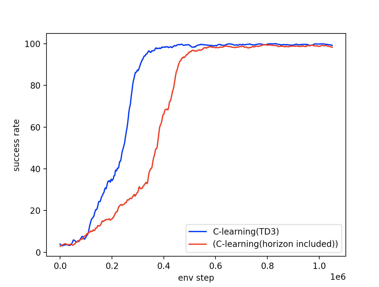
Refer to caption
Refer to caption
Figure 6: Success rate throughout training of C๐ถC-learning (blue) and naive horizon-aware Q๐‘„Q-learning (red) on FetchPickAndPlace-v1 (left); and C๐ถC-learning (blue) and C๐ถC-learning with uniform hโ„Žh sampling (red) on FetchPickAndPlace-v1 (right).

We also compare C๐ถC-learning against TDMs Pong etย al. (2018) for motion planning tasks. Results are in Figure 7. As mentioned in the main manuscript, TDMs assume a dense reward function, which C๐ถC-learning does not have access to. In spite of this, C๐ถC-learning significantly outperforms TDMs.
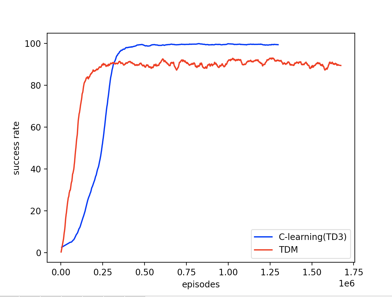
Refer to caption
Refer to caption
Figure 7: Success rate throughout training of C๐ถC-learning (blue) and TDMs (red) in FetchPickAndPlace-v1 (left) and HandManipulatePenFull-v0 (right).

Finally, we also compare against the non-cumulative version of C๐ถC-learning (A๐ดA-learning), and the discount-based recursion (D๐ทD-learning) in Dubinsโ€™ car. For D๐ทD-learning, we selected ฮณ๐›พ\gamma uniformly at random in [0,1]01[0,1]. Results are shown in table 4. We can see that indeed, C๐ถC-learning outperforms both alternatives. Curiously, while underperformant, A๐ดA-learning and D๐ทD-learning seem to obtain shorter paths among successful trials.

Table 4: Relevant metrics for the Dubinsโ€™ car environment, stratified by difficulty of goal (see Figure 5 (right) from appendix F). Runs in bold are either the best on the given metric in that environment, or have a mean score within the error bars of the best.
METHOD SUCCESS RATE PATH LENGTH
EASY MED HARD ALL EASY MED HARD ALL
C๐ถC-learning 97.44%ยฑ2.23%plus-or-minuspercent97.44percent2.23\mathbf{97.44\%\pm 2.23\%} 86.15%ยฑ4.06%plus-or-minuspercent86.15percent4.06\mathbf{86.15\%\pm 4.06\%} 81.14%ยฑ4.02%plus-or-minuspercent81.14percent4.02\mathbf{81.14\%\pm 4.02\%} 86.15%ยฑ2.44%plus-or-minuspercent86.15percent2.44\mathbf{86.15\%\pm 2.44\%} 6.66ยฑ0.91plus-or-minus6.660.916.66\pm 0.91 16.16ยฑ1.47plus-or-minus16.161.4716.16\pm 1.47 21.01ยฑ1.50plus-or-minus21.011.5021.01\pm 1.50 16.45ยฑ0.99plus-or-minus16.450.9916.45\pm 0.99
A๐ดA-learning 93.16%ยฑ3.20%plus-or-minuspercent93.16percent3.2093.16\%\pm 3.20\% 89.74ยฑ4.41%plus-or-minus89.74percent4.41\mathbf{89.74\pm 4.41\%} 62.88%ยฑ16.50%plus-or-minuspercent62.88percent16.5062.88\%\pm 16.50\% 78.12%ยฑ6.75%plus-or-minuspercent78.12percent6.7578.12\%\pm 6.75\% 5.84ยฑ0.59plus-or-minus5.840.59\mathbf{5.84\pm 0.59} 13.29ยฑ0.28plus-or-minus13.290.2813.29\pm 0.28 16.94ยฑ0.18plus-or-minus16.940.1816.94\pm 0.18 12.83ยฑ0.39plus-or-minus12.830.3912.83\pm 0.39
D๐ทD-learning 86.32%ยฑ12.27%plus-or-minuspercent86.32percent12.2786.32\%\pm 12.27\% 34.36%ยฑ15.71%plus-or-minuspercent34.36percent15.7134.36\%\pm 15.71\% 2.27%ยฑ3.21%plus-or-minuspercent2.27percent3.212.27\%\pm 3.21\% 30.21%ยฑ8.47%plus-or-minuspercent30.21percent8.4730.21\%\pm 8.47\% 5.62ยฑ0.25plus-or-minus5.620.25\mathbf{5.62\pm 0.25} 11.44ยฑ0.26plus-or-minus11.440.26\mathbf{11.44\pm 0.26} 13.97ยฑ0.00plus-or-minus13.970.00\mathbf{13.97\pm 0.00} 7.91ยฑ0.82plus-or-minus7.910.82\mathbf{7.91\pm 0.82}

Appendix G Experimental details

C-learning for stochastic environments: As mentioned in the main manuscript, we modify the replay buffer in order to avoid the bias incurred by HER sampling (Matthias etย al., 2018) in non-deterministic environments. We sample goals independently from the chosen episode. We sample gisubscript๐‘”๐‘–g_{i} to be a potentially reachable goal from sisubscript๐‘ ๐‘–s_{i} in hisubscriptโ„Ž๐‘–h_{i} steps. For example, if given access to a distance d๐‘‘d between states and goals such that the distance can be decreased at most by 111 unit after a single step, we sample gisubscript๐‘”๐‘–g_{i} from the set of g๐‘”gโ€™s such that dโ€‹(si,g)โ‰คhi๐‘‘subscript๐‘ ๐‘–๐‘”subscriptโ„Ž๐‘–d(s_{i},g)\leq h_{i}. Moreover, when constructing yisubscript๐‘ฆ๐‘–y_{i} (line 1 of algorithm 1), if we know for a fact that gisubscript๐‘”๐‘–g_{i} cannot be reached from siโ€ฒsubscriptsuperscript๐‘ โ€ฒ๐‘–s^{\prime}_{i} in hiโˆ’1subscriptโ„Ž๐‘–1h_{i}-1 steps, we output 00 instead of maxaโ€ฒโกCฮธโ€ฒโˆ—โ€‹(siโ€ฒ,aโ€ฒ,gi,hiโˆ’1)subscriptsuperscript๐‘Žโ€ฒsubscriptsuperscript๐ถsuperscript๐œƒโ€ฒsubscriptsuperscript๐‘ โ€ฒ๐‘–superscript๐‘Žโ€ฒsubscript๐‘”๐‘–subscriptโ„Ž๐‘–1\max_{a^{\prime}}C^{*}_{\theta^{\prime}}(s^{\prime}_{i},a^{\prime},g_{i},h_{i}-1). For example, dโ€‹(siโ€ฒ,gi)>hiโˆ’1๐‘‘subscriptsuperscript๐‘ โ€ฒ๐‘–subscript๐‘”๐‘–subscriptโ„Ž๐‘–1d(s^{\prime}_{i},g_{i})>h_{i}-1 allows us to set yi=0subscript๐‘ฆ๐‘–0y_{i}=0. We found this practice, combined with the sampling of gisubscript๐‘”๐‘–g_{i} described above, to significantly improve performance. While this requires some knowledge of the environment, for example a metric over states, this knowledge is often available in many environments. For frozen lake, we use the L1subscript๐ฟ1L_{1} metric to determine if a goal is not reachable from a state, while ignoring the holes in the environment so as to not use too much information about the environment.

G.1 Frozen lake

For all methods, we train for 300300300 episodes, each one of maximal length 505050 steps, we use a learning rate 10โˆ’3superscript10310^{-3}, a batch size of size 256256256, and train for 646464 gradient steps per episode. We use a 0.10.10.1-greedy for the behavior policy. We use a neural network with two hidden layers of respective sizes 606060 and 404040 with ReLU activations. We use 151515 fully random exploration episodes before we start training. We take pโ€‹(s0)๐‘subscript๐‘ 0p(s_{0}) as uniform among non-hole states during training, and set it as a point mass at (1,0)10(1,0) for testing. We set pโ€‹(g)๐‘๐‘”p(g) as uniform among states during training, and we evaluate at every goal during testing. For C๐ถC-learning, we use ฮบ=3๐œ…3\kappa=3, and copy the target network every 101010 steps. We take the metric d๐‘‘d to be the L1subscript๐ฟ1L_{1} norm, completely ignoring the holes so as to not use too much environment information. For the horizon-independent policy, we used โ„‹={1,2,โ€ฆ,50}โ„‹12โ€ฆ50\mathcal{H}=\{1,2,\dots,50\} and ฮฑ=0.9๐›ผ0.9\alpha=0.9. We do point out that, while C๐ถC-learning did manage to recover the safe path for large hโ„Žh, it did not do always do so: we suspect that the policy of going directly up is more likely to be explored. However, we never observed GCSL taking the safe path.

G.2 Mini maze

We again train for 300030003000 episodes, now of maximal length 200200200. We train 323232 gradient steps per episode, and additionally decay the exploration noise of the C๐ถC-learning behavior policy throughout training according to ฯต=0.5/(1+nGโ€‹D/1000)italic-ฯต0.51subscript๐‘›๐บ๐ท1000\epsilon=0.5/(1+n_{GD}/1000). The network we used has two hidden layers of size 200200200 and 100100100 with ReLU activations, respectively. While the environment is deterministic, we use the same replay buffer as for frozen lake, and take the metric d๐‘‘d to be the L1subscript๐ฟ1L_{1} norm, completely ignoring walls. We found this helped improve performance and allowed C๐ถC-learning to still learn to reach far away goals. We also define โ„‹โ€‹(s,g)โ‰”{โ€–sโˆ’gโ€–1,โ€–sโˆ’gโ€–1+1,โ€ฆ,hmax}โ‰”โ„‹๐‘ ๐‘”subscriptnorm๐‘ ๐‘”1subscriptnorm๐‘ ๐‘”11โ€ฆsubscriptโ„Žmax\mathcal{H}(s,g)\coloneqq\{\|s-g\|_{1},\|s-g\|_{1}+1,\ldots,h_{\text{max}}\}, with hmaxโ‰”50โ‰”subscriptโ„Žmax50h_{\text{max}}\coloneqq 50, as the set of horizons over which we will check when rolling out the policies. We take pโ€‹(s0)๐‘subscript๐‘ 0p(s_{0}) as a point mass both for training and testing. We use pโ€‹(g)๐‘๐‘”p(g) during training as specified in Algorithm 1, and evaluate all the methods on a fixed set of goals. Additionally, we lower the learning rate by a factor of 101010 after 200020002000 episodes. All the other hyperparameters are as in frozen lake. Figure 5 shows the split between easy, medium, and hard goals.

G.3 Dubinsโ€™ car

We train for 450045004500 episodes, each one with a maximal length of 100100100 steps and using 808080 gradient steps per episode. We use a neural network with two hidden layers of respective sizes 400400400 and 300300300 with ReLU activations. We take the metric d๐‘‘d to be the Lโˆžsubscript๐ฟL_{\infty} norm, completely ignoring walls, which we only use to decide whether or not we have reached the goal. We take pโ€‹(s0)๐‘subscript๐‘ 0p(s_{0}) as a point mass both for training and testing. We use pโ€‹(g)๐‘๐‘”p(g) during training as specified in Algorithm 1, and evaluate all the methods on a fixed set of goals. All other hyperparameters are as in frozen lake. The partition of goals into easy, medium and hard is specified in Figure 5, where the agent always starts at the upper left corner.

G.4 FetchPickAndPlace-v1

We train with a learning rate of 0.0001 and batch size of 256. We take 646464 gradient steps per episode, and only update ฯ•italic-ฯ•\phi with half the frequency of ฮธ๐œƒ\theta. We use 400004000040000 episodes for FetchPickAndPlace-v1. All the other hyperparameters are as in Dubinsโ€™ car.

G.5 HandManipulatePenFull-v0

We train with a learning rate of 0.0001 and batch size of 256. We take 808080 gradient steps per episode, and only update ฯ•italic-ฯ•\phi with half the frequency of ฮธ๐œƒ\theta. We use 600006000060000 episodes for HandManipulatePenFull-v0. All the other hyperparameters are as in Dubinsโ€™ car.