A Fixed-Time Stable Adaptation Law for Safety-Critical Control under Parametric Uncertainty

Abstract

We present a novel technique for solving the problem of safe control for a general class of nonlinear, control-affine systems subject to parametric model uncertainty. Invoking Lyapunov analysis and the notion of fixed-time stability (FxTS), we introduce a parameter adaptation law which guarantees convergence of the estimates of unknown parameters in the system dynamics to their true values within a fixed-time independent of the initial parameter estimation error. We then synthesize the adaptation law with a robust, adaptive control barrier function (RaCBF) based quadratic program to compute safe control inputs despite the considered model uncertainty. To corroborate our results, we undertake a comparative case study on the efficacy of this result versus other recent approaches in the literature to safe control under uncertainty, and close by highlighting the value of our method in the context of an automobile overtake scenario.

I Introduction

Safe control design in our increasingly technology-reliant society is important, yet difficult even under idealized conditions. In theory, it may be performed by a variety of techniques, including control barrier function (CBF)-based strategies [1, 2]. As a set-theoretic method for enforcing that the states of a system remain safe, i.e. within a specified set, CBFs have proven to be effective both in correcting some potentially unsafe control action [3, 4] and as a constraint in optimization-based control [5, 6]. In fact, control design using quadratic programs (QP) as a means to synthesize control Lyapunov function (CLF)-based performance specifications, which can guarantee convergence of the closed-loop trajectories to some goal set, and CBF-based safety has become a staple in the literature [7, 8].

While CLFs encode a goal-reaching performance specification, the rate of convergence depends on the form of the condition imposed on its time-derivative. For example, while an exponentially stable CLF [9] guarantees that system trajectories reach a goal set as time tends toward infinity, the principle of fixed-time stability (FxTS) is used to define a fixed-time stable CLF [6] which drives the closed-loop trajectories to the goal within a fixed-time independent of initial conditions.

Robust approaches to safety [10], which often shrink the safe set in order to preserve set-invariance in the presence of worst-case disturbances, tend to be overly conservative. Typically, conservatism degrades the ability of the controller to meet performance objectives. In contrast, adaptive safety techniques [11] are prone to chattering control solutions, especially as the state approaches the boundary of the safe set. While a highly oscillatory control signal may suffice in simulation, it can destabilize dynamical systems in practice. In an approach which combines these two regimes, however, the authors of [12] demonstrate that robust, adaptive control barrier functions (RaCBF) can mitigate these shortcomings. In addition, they utilize set-membership identification (SMID) to reduce the uncertainty surrounding a set of unknown parameters in the system dynamics, which results in improved performance. In a learning-based approach, [13] seeks to improve the performance of a Segway controller by learning unstructured uncertainty in the dynamics of the control barrier function itself. And while many of these techniques have been demonstrably effective in improving controller performance, the issue of navigating the domain near the boundary of the safe region remains problematic without formal guarantees of deciphering model uncertainty.

In considering some structured, parametric uncertainty for a class of nonlinear, control-affine systems, we introduce a novel parameter adaptation law which provides such a guarantee to drive the parameter estimates to their true values within fixed-time, independent of the initial estimates. Using Lyapunov analysis, we leverage this result to define an upper bound on the parameter estimation error as an explicit function of time. We then introduce a new condition on the time derivative of an RaCBF that guarantees forward-invariance of a shrunken safe set, which approaches the nominal safe set within the fixed-time horizon. In a case study on the ability of our proposed controller to tolerate marginally safe regions of the state space versus a selection from the literature, we compare the works of [11, 12, 5] and [14] on a simple problem with static obstacles. Finally, we use an automobile overtaking scenario to highlight another advantage of the proposed method: with the uncertain parameters in the system dynamics guaranteed to be known within fixed-time, our controller can accomplish a maneuver even under high levels of uncertainty.

The paper is organized as follows. Section II reviews set invariance via CBFs, finite-time stability (FTS), FxTS, and an FTS parameter estimation scheme from the literature. In Section III we formalize the problem at hand. Section IV contains our novel FxTS adaptation law and its implications on safe control under uncertainty. Section V highlights a simple case study used to compare other recent work to our proposed method, and its application on a highway overtake example. We conclude with a summary of contributions and directions for future work in Section VI.

II Mathematical Preliminaries

In the rest of the paper, $\mathbb{R}$ denotes the set of real numbers. The ones vector of size $n\times m$ is denoted $\mathbf{1}_{n\times m}$. We use $\|\cdot\|$ to denote the Euclidean norm and $\|\cdot\|_{\infty}$ to denote the $\mathscr{L}_{\infty}$ norm. As convention, we denote the minimum and maximum eigenvalue of a matrix $M$ as $\lambda_{min}(M)$ and $\lambda_{max}(M)$ respectively. We write $\partial S$ for the boundary of the closed set $S$, and $\textrm{int}(S)$ for its interior. The Lie derivative of a function $V:\mathbb{R}^{n}\rightarrow\mathbb{R}$ along a vector field $f:\mathbb{R}^{n}\rightarrow\mathbb{R}^{n}$ at a point $x\in\mathbb{R}^{n}$ is denoted as $L_{f}V(x)\triangleq\frac{\partial V}{\partial x}f(x)$.

We now review the preliminaries, including a finite-time parameter adaptation law from the literature which inspired our fixed-time adaptation law.

II-A Set Invariance

In this paper, we consider the following class of nonlinear, control-affine systems subject to parametric uncertainty:

$$\dot{x}(t) =f(x(t))+g(x(t))u(t)+\Delta(x(t))\theta,\;\;x(t_{0})=x_{0},$$ (1)

where $x(t)\in\mathbb{R}^{n}$ denotes the state, $u(t)\in U\subset\mathbb{R}^{m}$ the control input, and $\theta\in\Theta\subset\mathbb{R}^{p}$ some constant, bounded, unknown parameters. We assume that $f:\mathbb{R}^{n}\rightarrow\mathbb{R}^{n}$ and $g:\mathbb{R}^{n}\rightarrow\mathbb{R}^{n\times m}$ are locally Lipschitz, that $\Delta:\mathbb{R}^{n}\rightarrow\mathbb{R}^{n\times p}$ is a known regressor matrix, and that $f$, $g$, and $\Delta$ are bounded for bounded inputs. The regressor $\Delta$ may capture, for example, the effects of sensing or modelling errors in the system dynamics, whereas the $\theta$ vector parameterizes such errors. We also define $\hat{\theta}$ as the estimated parameter vector, and $\tilde{\theta}=\theta-\hat{\theta}$ as the parameter estimation error vector. As such, the parameter error dynamics are described by

$$\dot{\tilde{\theta}}=\dot{\theta}-\dot{\hat{\theta}}=-\dot{\hat{\theta}},\;\;\tilde{\theta}(0)=\tilde{\theta}_{0}.$$ (2)

Let us also define a set of safe states as

$$S =\left\{x\in\mathbb{R}^{n}:h(x)\geq 0\right\}$$ (3a)

$$\partial S =\left\{x\in\mathbb{R}^{n}:h(x)=0\right\}$$ (3b)

$$\textrm{int}(S) =\left\{x\in\mathbb{R}^{n}:h(x)>0\right\}$$ (3c)

where $h:\mathbb{R}^{n}\rightarrow\mathbb{R}$ is continuously differentiable. Then, the following Lemma, known as Nagumo’s Theorem [15], provides a necessary and sufficient condition on the forward invariance of the set (3) under the system dynamics (1).

Lemma 1.

Let a unique closed-loop solution to (1) exist in forward time. We say that the set $S$ can be rendered forward-invariant if and only if there exists a control $u\in U$ such that

$$\sup_{u\in U}\{L_{f}h(x)+L_{g}h(x)u+L_{\Delta}h(x)\theta\}\geq 0,\forall x\in\partial S.$$ (4)

Remark 1.

The closed-loop system (1) admits a unique solution if $u(t)\in U$ is Lipschitz.

The authors of [12] ensure $S$ is safe with respect to the uncertain dynamics (1) by enforcing that a shrunken set, $S_{r}$, is safe. Before formally defining $S_{r}$ we make the following assumption.

Assumption 1.

The set $\Theta$ to which the unknown parameters $\theta$ belong is known, compact, and convex.

Remark 2.

Assumption 1 imples that we can also restrict $\hat{\theta}\in\Theta$. Thus, we can define an upper bound $\vartheta\coloneqq\sup_{\theta_{1},\theta_{2}\in\Theta}(\|\theta_{1}-\theta_{2}\|_{\infty})$ on the norm $\|\tilde{\theta}\|_{\infty}$ of the parameter estimation error $\tilde{\theta}$, so that $\|\tilde{\theta}\|_{\infty}\leq\vartheta.$

We let $\bm{\vartheta}=\vartheta\cdot\mathbf{1}_{p\times 1}$, and are now ready to present the definition for the shrunken set, $S_{r}$, as defined in [12].

$$S_{r} =\left\{x\in\mathbb{R}^{n}:h(x)\geq\frac{1}{2}\bm{\vartheta}^{T}\Gamma^{-1}\bm{\vartheta}\right\}$$ (5a)

$$\partial S_{r} =\left\{x\in\mathbb{R}^{n}:h(x)=\frac{1}{2}\bm{\vartheta}^{T}\Gamma^{-1}\bm{\vartheta}\right\}$$ (5b)

$$\textrm{int}(S_{r}) =\left\{x\in\mathbb{R}^{n}:h(x)>\frac{1}{2}\bm{\vartheta}^{T}\Gamma^{-1}\bm{\vartheta}\right\}$$ (5c)

where $\Gamma$ is a constant, positive-definite matrix such that $h(x(0))\geq\frac{1}{2}\bm{\vartheta}^{T}\Gamma^{-1}\bm{\vartheta}$. A new CBF may be defined as

$$h_{r}(x,\bm{\vartheta})=h(x)-\frac{1}{2}\bm{\vartheta}^{T}\Gamma^{-1}\bm{\vartheta},$$ (6)

and the sufficient condition that renders $S_{r}$ safe is

$$\dot{h}_{r}=\frac{\partial h}{\partial x}\dot{x}-\bm{\vartheta}^{T}\Gamma^{-1}\dot{\bm{\vartheta}}\geq-\alpha(h_{r}),$$ (7)

where $\alpha:[0,a)\rightarrow[0,\infty)$ is some class $K$ function, i.e., strictly increasing with $\alpha(0)=0$.

Remark 3.

If $S_{r}\subset S$ in (5) is safe, then $S$ in (3) is safe. Thus, satisfaction of (7) implies that (4) holds.

II-B Finite- and Fixed-Time Stability

We now address performance criteria: finite- and fixed-time stability of an equilibrium point of the dynamical system

$$\dot{x}(t) =f(x(t)),\quad x(t_{0})=x_{0},$$ (8)

for which it is assumed that a unique solution exists, where $x\in\mathbb{R}^{n}$, $f:\mathbb{R}^{n}\rightarrow\mathbb{R}^{n}$ is continuous, and $f(0)=0$.

Definition 1 ([16]).

The origin of (8) is globally finite-time stable (FTS) if the following conditions hold:

• The origin of (8) is stable in the sense of Lyapunov

• Any solution $x(t,x_{0})$ of (8) reaches the origin in finite settling-time, $T(x_{0})$, i.e. $x(t,x_{0})=0$, $\forall t\geq T(x_{0})$.

Definition 2 ([17]).

The origin of (8) is fixed-time stable (FxTS) if it is globally FTS and any solution $x(t,x_{0})$ of (8) reaches the origin in finite settling-time, $T$, independent of $x_{0}$, i.e. $x(t,x_{0})=0$, $\forall t\geq T$.

We refer the interested reader to [16] and [17] respectively for Lyapunov conditions which guarantee FTS and FxTS of the origin of (8).

II-C Finite-Time Parameter Estimation

The parameter estimation scheme in the discussion to follow is predicated on Assumption 2.

Assumption 2.

The state, $x$, and control input $u$, of (1) are bounded, and $x$ is accessible for measurement.

Let us now review the notion of persistent excitation (PE).

Definition 3 ([18]).

A vector or matrix function, $\phi$, is persistently excited (PE) if there exist $T>0$, $\epsilon>0$, such that $\int_{t}^{t+T}\phi(r)\phi^{T}(r)dr\geq\epsilon I,\forall t\geq 0$.

Now we introduce the following assumption on $\Delta(x)$.

Assumption 3.

The transpose of the regressor matrix in (1), $\Delta^{T}(x)$, is persistently excited.

Remark 4.

Positive-definiteness of $\Delta^{T}\Delta$ is sufficient for $\Delta^{T}$ to satisfy the PE condition.

We now review a FTS parameter estimation scheme which forms the basis for our FxTS adaptation law and was first proposed for nonlinear dynamical systems in [19], and extended for robotic applications in [20]. First, we note that we may re-write (1) as:

$$\dot{x}(t) =\varphi(x,u)+\Phi(x)\theta,$$ (9)

where $\varphi(x,u)=f(x)+g(x)u$ and $\Phi(x)=\Delta(x)$. The authors of [19] and [20] introduce $x_{f}$, $\varphi_{f}$, and $\Phi_{f}$ to filter $x$, $\varphi$, and $\Phi$ as follows:

$$k\dot{x}_{f}+x_{f} =x,\quad x_{f}(0)=0,\quad\dot{x}_{f}(0)=0$$ (10)

$$k\dot{\varphi}_{f}+\varphi_{f} =\varphi,\quad\varphi_{f}(0)=0,\quad\dot{\varphi}_{f}(0)=0$$ (11)

$$k\dot{\Phi}_{f}+\Phi_{f} =\Phi,\quad\Phi_{f}(0)=0,\quad\dot{\Phi}_{f}(0)=0$$ (12)

where $k>0$ is a design parameter. Mimicking the form of the system dynamics, the filtered system dynamics are:

$$\dot{x}_{f}=\varphi_{f}+\Phi_{f}\theta,$$ (13)

which serves as the basis for estimating $\theta$. We now observe that $\dot{x}_{f}-\varphi_{f}=\Phi_{f}\theta$ and define an auxiliary and integrated regressor matrix $P$ and vector $Q$ such that:

$$\dot{P} =-\ell_{e}P+\Phi_{f}^{T}\Phi_{f},\quad P(0) =0$$ (14)

$$\dot{Q} =-\ell_{e}Q+\Phi_{f}^{T}(\dot{x}_{f}-\varphi_{f}),\quad Q(0) =0$$ (15)

where $\ell_{e}>0$ is another design parameter. The solutions are:

$$P(t) =\int_{0}^{t}e^{-\ell_{e}(t-r)}\Phi_{f}^{T}(r)\Phi_{f}(r)dr$$ (16)

$$Q(t) =\int_{0}^{t}e^{-\ell_{e}(t-r)}\Phi_{f}^{T}(r)(\dot{x}_{f}(r)-\varphi_{f}(r))dr$$ (17)

and from them it may be discerned that $Q=P\theta$. Now, define an additional auxiliary vector as

$$W=P\hat{\theta}-Q=-P\tilde{\theta}.$$ (18)

Then, the authors of [20] introduce their adaptation law as

$$\dot{\hat{\theta}}=-\Lambda\frac{P^{T}W}{\|W\|},$$ (19)

where $\Lambda$ is a constant, positive definite, gain matrix. Finite-time (FT) convergence of the estimated parameters to their true values is guaranteed by the following result.

Theorem 1 ([20]).

For system (9) with parameter adaptation law (19) and $\lambda_{min}(P)>\sigma>0$, the parameter estimation error $\tilde{\theta}$ converges to zero in finite-time $t_{a}$, satisfying $t_{a}\leq\|\tilde{\theta}(0)\|\frac{\lambda_{max}(\Gamma^{-1})}{\sigma}$.

While in general it is not required that $\Lambda$ from (19) and $\Gamma$ from (5) be equivalent, we consider this to be true for the rest of the paper. In Section IV, we advance the FT parameter estimation result by proposing a FxTS adaptation law for the class of systems described by (1).

III Problem Formulation

We now formalize the problem under consideration.

Problem 1.

Consider a nonlinear, control-affine dynamical system subject to parametric uncertainty as in (1). Given that Assumptions 1-3 hold, design an adaptation law, $\dot{\hat{\theta}}$, and controller, $u$, such that the following conditions are satisfied:

1. The parameter estimation error converges to zero within fixed-time, $T_{\theta}$, i.e. $\tilde{\theta}(t)\rightarrow 0$ as $t\rightarrow T_{\theta}<\infty$, independent of $\tilde{\theta}(0)$.

2. The system trajectories remain safe for all time, i.e. $x(t)\in S$, $\forall t\geq t_{0}$.

3. The system trajectories converge to a goal set within fixed-time, $T_{g}$, i.e. $x(t)\in S_{g}$, $\forall t\geq T_{g}$.

The following section contains our proposed method.

IV Main Results

Before introducing one of the main results of the paper, we address modifications to the filtering scheme (10)-(12). In place of the first-order scheme of [19],[20], we use the following second-order filters:

$$k_{e}^{2}\ddot{x}_{f}+2k_{e}\dot{x}_{f}+x_{f} =x$$ (20)

$$k_{e}^{2}\ddot{\varphi}_{f}+2k_{e}\dot{\varphi}_{f}+\varphi_{f} =\varphi$$ (21)

$$k_{e}^{2}\ddot{\Phi}_{f}+2k_{e}\dot{\Phi}_{f}+\Phi_{f} =\Phi$$ (22)

where all initial conditions are zero, i.e. $\beta_{f}(0)=0$, $\dot{\beta}_{f}(0)=0$, $\ddot{\beta}_{f}(0)=0$, $\forall\beta\in\{x,\varphi,\Phi\}$. This second-order system is stable, strictly proper, and minimum-phase similarly to (10)-(12), and in addition, it is critically damped with a natural frequency of $\omega_{n}=1/k_{e}$. This is desirable, as critically damped systems exhibit the smallest settling time, $t_{s}$, without oscillations [21].

IV-A FxTS Adaptation Law

We now introduce one of the main results of the paper, an adaptation law which renders the trajectories $\tilde{\theta}(t)$ of the parameter estimation error fixed-time stable to zero, and thus guarantees convergence of the parameters to their true values within fixed-time.

Theorem 2.

Consider a nonlinear, control-affine system with parametric uncertainty as in (1). If (20)-(22) filter $x$, $\varphi$, and $\Phi$, and the auxiliary matrix P and vectors Q, W are defined by (14)-(18), then, under the ensuing adaptation law

$$\dot{\hat{\theta}}=\Gamma W\left(W^{T}P^{-T}W\right)^{-1}\left(-c_{1e}\nu^{\gamma_{1e}}-c_{2e}\nu^{\gamma_{2e}}\right),$$ (23)

the estimated parameters, $\hat{\theta}(t)$, converge to the true parameters, $\theta$, in fixed-time, $T_{\theta}$, i.e., $\tilde{\theta}(t)\rightarrow 0$ and $\hat{\theta}(t)\rightarrow\theta$ as $t\rightarrow T_{\theta}$, where

$$T_{\theta}\leq T_{b}=\frac{1}{c_{1e}(1-\gamma_{1e})}+\frac{1}{c_{2e}(\gamma_{2e}-1)}.$$ (24)

with $\nu=\frac{1}{2}W^{T}P^{-T}\Gamma^{-1}P^{-1}W$, $c_{1e}>0$, $c_{2e}>0$, $0<\gamma_{1e}<1$, $\gamma_{2e}>1$, and $\Gamma\in\operatorname{\mathbb{R}}^{p\times p}$ being a constant, positive-definite, gain matrix.

Proof.

Consider the Lyapunov function candidate $V_{\tilde{\theta}}=\frac{1}{2}\tilde{\theta}^{T}\Gamma^{-1}\tilde{\theta}$ for the system of the parameter-error dynamics (2). Since $\dot{\theta}=0$, its time derivative along the trajectories of (2) reads $\dot{V}_{\tilde{\theta}}=-\tilde{\theta}^{T}\Gamma^{-1}\dot{\hat{\theta}}$. Applying the adaptation law (23) yields $\dot{V}_{\tilde{\theta}}=-\tilde{\theta}^{T}W\left(W^{T}P^{-T}W\right)^{-1}\left(-c_{1e}\nu^{\gamma_{1e}}-c_{2e}\nu^{\gamma_{2e}}\right)$. Then, by substituting (18), we obtain

$$\dot{V}_{\tilde{\theta}}=-c_{1e}V_{\tilde{\theta}}^{\gamma_{1e}}-c_{2e}V_{\tilde{\theta}}^{\gamma_{2e}},$$ (25)

i.e., the fixed-time stability condition from [17, Lemma 1]. Hence, the origin of (2) is fixed-time stable, and the trajectories $\tilde{\theta}(t)$ reach the origin within a settling time $T_{\theta}$, given by (24). Consequently, the estimated parameter vector, $\hat{\theta}(t)$, converges to the true parameter vector, $\theta$, within a fixed time, $T_{\theta}$, i.e., $\hat{\theta}(T_{\theta})=\theta$. ∎

Whereas previous studies (e.g. [22]) use (14) and (15) in the design of a FxT adaptation scheme that converges to some bounded set, (23) guarantees fixed-time convergence of the estimated parameters to their true values. With this knowledge, we derive an expression for the upper bound on the infinity norm of the parameter error as a function of time.

Corollary 1.

Let $\tilde{\theta}=\theta-\hat{\theta}$ be the parameter estimation error vector associated with a system of the form (1). If all of the following conditions hold

1. The estimated parameter update law, $\dot{\hat{\theta}}$, is given by (23)

2. $u(x(t))$ is any locally Lipschitz controller

3. $\Gamma$ is constant, positive-definite, and diagonal

4. $\gamma_{1e}=1-\frac{1}{\mu_{e}}$ and $\gamma_{2e}=1+\frac{1}{\mu_{e}}$ for some $\mu_{e}>1$

then the following expression constitutes an upper bound on $\|\tilde{\theta}(t)\|_{\infty},\;\forall t\in[0,T_{\theta}]$:

$$\|\tilde{\theta}(t)\|_{\infty}\leq\sqrt{M\left(\frac{1}{N}\tan{\left[\Xi-N\frac{c_{1e}}{\mu_{e}}t\right]}\right)^{\mu_{e}}}\coloneqq\eta(t),$$ (26)

where $M=2\lambda_{max}(\Gamma)$, $N=\sqrt{\frac{c_{2e}}{c_{1e}}}$, and

$$\Xi=\tan^{-1}{\left(\frac{1}{2}N\bm{\eta}^{T}(0)\Gamma^{-1}\bm{\eta}(0)\right)}$$ (27)

with $\bm{\eta}(t)=\eta(t)\cdot\mathbf{1}_{p\times 1}$ and

$$T_{\theta}\leq\frac{\mu_{e}\Xi}{\sqrt{c_{1e}c_{2e}}}\leq T_{b}$$ (28)

Proof.

We consider the Lyapunov function candidate $V_{\tilde{\theta}}=\frac{1}{2}\tilde{\theta}^{T}\Gamma^{-1}\tilde{\theta}$, whose time derivative along the trajectories of (2) reads $\frac{dV_{\tilde{\theta}}}{dt}=-c_{1e}V_{\tilde{\theta}}^{1-1/\mu_{e}}-c_{2e}V_{\tilde{\theta}}^{1+1/\mu_{e}}$.

By separation of variables and integration, we now solve for $t$ as a function of $V(0)$ and $V(t)$. The change of variables $x=V_{\tilde{\theta}}^{1/\mu_{e}}$ and $dx=\frac{1}{\mu_{e}}V_{\tilde{\theta}}^{1-1/\mu_{e}}dV$ allows us to obtain:

$$t=\int_{V(0)}^{V(t)}\frac{\mu_{e}x^{\mu_{e}-1}dx}{-c_{1e}x^{\mu_{e}-1}-c_{2e}x^{\mu_{e}+1}}=$$ (29)

$$-\frac{\mu_{e}}{\sqrt{c_{1e}c_{2e}}}\left[\tan^{-1}\left(NV_{\tilde{\theta}}^{1/\mu_{e}}(t)\right)-\tan^{-1}\left(NV_{\tilde{\theta}}^{1/{\mu_{e}}}(0)\right)\right]$$

where $N=\sqrt{\frac{c_{2e}}{c_{1e}}}$. This leads to

$$V_{\tilde{\theta}}(t) =\left(\frac{1}{N}\tan\left[\tan^{-1}\left(NV(0)\right)-N\frac{c_{1e}}{\mu_{e}}t\right]\right)^{\mu_{e}}$$ (30)

where $V(0)=\frac{1}{2}\tilde{\theta}(0)^{T}\Gamma^{-1}\tilde{\theta}(0)\leq\frac{1}{2}\bm{\eta}(0)^{T}\Gamma^{-1}\bm{\eta}(0)$. Now, since $V_{\tilde{\theta}}=\frac{1}{2}\tilde{\theta}^{T}\Gamma^{-1}\tilde{\theta}$, then with $\Gamma$ diagonal we can express $V_{\tilde{\theta}}=\frac{1}{2}(\Gamma^{-1}_{11}\tilde{\theta}_{1}^{2}+...+\Gamma^{-1}_{pp}\tilde{\theta}_{p}^{2})$, and observe that $V_{\tilde{\theta}}\geq\frac{1}{2}\lambda^{-1}_{max}(\Gamma)\|\tilde{\theta}\|^{2}\geq\frac{1}{2}\lambda^{-1}_{max}(\Gamma)\|\tilde{\theta}\|_{\infty}^{2}$. Then, we substitute (30) in this inequality and rearrange terms to recover (26).

Then, for $0\leq t\leq\frac{\mu_{e}}{c_{1e}N}\textrm{tan}^{-1}\left(\frac{1}{2}N\bm{\eta}^{T}\Gamma^{-1}\bm{\eta}\right)$ we have that (30) decreases monotonically to zero. As such, we let $\Xi=\textrm{tan}^{-1}\left(\frac{1}{2}N\bm{\eta}^{T}\Gamma^{-1}\bm{\eta}\right)$ and obtain (28), which places a tighter upper bound on the settling time, $T_{\theta}$, than (24). ∎

Remark 5.

As a consequence of (26), we may tighten the set of admissible parameters at time $t$ as $\Theta(t)=\{\theta\in\mathbb{R}^{p}:\;\|\theta-\hat{\theta}(t)\|_{\infty}\leq\eta(t)\}$, $\forall t\in[0,T_{\theta}]$, and as $\Theta(t)=\{\hat{\theta}\}$, $\forall t\in(T_{\theta},\infty]$.

We now formalize the new RaCBF condition for forward-invariance of sets $S$ and $S_{r}$, defined in (3) and (5).

Theorem 3.

Let $\bm{\eta}(t)=\eta(t)\cdot\mathbf{1}_{p\times 1}$ where $\eta(t)$ is given by (26). Under the premises of Corollary 1, the following condition is sufficient for forward-invariance of $S_{r}$, i.e. (5):

$$\sup_{u\in U}\{L_{f}h(x)+L_{g}h(x)u+\Psi\}$$

$$\geq-\alpha\left(h(x)-\frac{1}{2}\bm{\eta}(t)^{T}\Gamma^{-1}\bm{\eta}(t))\right)+\mathrm{Tr}(\Gamma^{-1})\eta(t)\dot{\eta}(t)$$ (31)

where

$$\dot{\eta}(t) =Z\tan^{\frac{\mu_{e}}{2}-1}\left(\Xi-N\frac{c_{1e}}{\mu_{e}}t\right)\sec^{2}\left(\Xi-N\frac{c_{1e}}{\mu_{e}}t\right)$$ (32)

$$\Psi =\sum_{i=1}^{p}\min\left\{C_{i}P_{\Theta}(\hat{\theta}_{i}-\eta),C_{i}P_{\Theta}(\hat{\theta}_{i}+\eta)\right\}$$ (33)

for $Z=-c_{1e}\sqrt{MN^{2-\mu_{e}}}$, where $C_{i}$ denotes the $i^{th}$ column of $L_{\Delta}h(x)$ for $i\in\{1,\ldots,p\}$, and $P_{\Theta}$ the vector projection onto $\Theta$, as defined in [23].

Proof.

We recall (6) and now replace the constant $\bm{\vartheta}$ with the time-varying $\bm{\eta}(t)$, where henceforth we drop the argument. Thus, $h_{r}(x,\bm{\eta})=h(x)-\frac{1}{2}\bm{\eta}^{T}\Gamma^{-1}\bm{\eta}$, and $\dot{h}_{r}(x,\bm{\eta})=\frac{\partial h_{r}}{\partial x}\dot{x}+\frac{\partial h_{r}}{\partial\bm{\eta}}\dot{\bm{\eta}}$. We will show that if (3) holds then (7) holds and thus (5) is forward-invariant.

First, $\frac{\partial h_{r}}{\partial x}\dot{x}=\frac{\partial h}{\partial x}\dot{x}=L_{f}h(x)+L_{g}h(x)u+L_{\Delta}h(x)\theta$, then with $\Gamma$ diagonal we can express $\frac{\partial h_{r}}{\partial\bm{\eta}}\dot{\bm{\eta}}=-\bm{\eta}^{T}\Gamma^{-1}\dot{\bm{\eta}}=-\mathrm{Tr}(\Gamma^{-1})\eta\dot{\eta}$, where we obtain $\dot{\eta}(t)$ in (32) by differentiating (26) from Corollary 1.

Next, we consider the case where $(\bm{\eta}+\hat{\theta})\in\Theta$, for which $P_{\Theta}(\bm{\eta}+\hat{\theta})=(\bm{\eta}+\hat{\theta})$. By (26) we have that $\hat{\theta}_{i}-\eta\leq\theta_{i}\leq\hat{\theta}_{i}+\eta$, $\forall i\in\{1,\ldots,p\}$, where $\Theta$ is convex by Assumption 1. Thus, the solution of the following minimization problem represents the worst admissible effect of the unknown parameters on safety:

$$\phi^{*}=\operatorname*{arg\,min}_{\phi\in\Theta}L_{\Delta}h(x)\phi$$ (34)

This is a constrained linear program. As such, a unique minimizer, $\phi^{*}=[\phi_{1}^{*}\;\ldots\;\phi_{p}^{*}]^{T}$ exists, where by the fact that $L_{\Delta}h(x)\phi=\sum_{i=1}^{p}C_{i}\phi_{i}$ with $C_{i}$ as the i^th column of $L_{\Delta}h(x)$, we have that $\phi_{1}^{*},\;\ldots\;,\phi_{p}^{*}$ are the minimizers of the following $p$ constrained linear programs:

$$\phi_{i}^{*}=\operatorname*{arg\,min}_{\hat{\theta}_{i}-\eta\leq\phi_{i}\leq\hat{\theta}_{i}+\eta}C_{i}\phi_{i},\quad\forall i\in\{1,\ldots,p\}$$ (35)

Furthermore, the solutions of constrained linear programs are guaranteed to be on the boundary of the solution domain, which in this case implies that either $\phi_{i}^{*}=\hat{\theta}_{i}-\eta$ or $\phi_{i}^{*}=\hat{\theta}_{i}+\eta$. Thus, we denote $\Psi=L_{\Delta}h(x)\phi^{*}$ and recover (33) so that $\Psi\leq L_{\Delta}h(x)\theta$, $\forall\theta\in\Theta$.

For $(\bm{\eta}+\hat{\theta})\notin\Theta$, (34) is again solved, but now $P_{\Theta}(\bm{\eta}+\hat{\theta})$ reduces $\eta$ when necessary to enforce that $\phi\in\Theta$. We again obtain that a unique solution exists and that $\Psi\leq L_{\Delta}h(x)\theta$, $\forall\theta\in\Theta$.

For both cases we have that $L_{f}h(x)+L_{g}h(x)u+\Psi\leq\frac{\partial h}{\partial x}\dot{x}$ and thus (3) implies (7), and (5) is forward-invariant. ∎

The use of the projection operator in Theorem 3 reduces the conservatism of the approach without compromising the robustness of the forward-invariance condition.

V Case Study

V-A Comparing Controllers

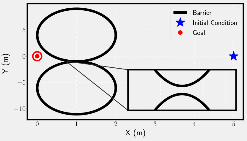
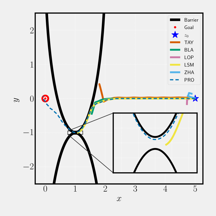
In the first numerical study, we investigate how our approach compares to other recent results in the literature, namely the adaptation laws from [11], [12], and [14], and the worst-case disturbance consideration of [5]. As a basis for comparison, we consider a 2D single-integrator system subject to parametric uncertainty and challenge the controllers to safely achieve convergence to the origin by avoiding static obstacles separated by a small gap (Fig. 1).

Figure 1: Problem setup for the first numerical case study, ”Shoot the Gap.” The controller must determine what actions, $u_{x}$ and $u_{y}$, to take in order to realize safe trajectories from the Initial Condition to the Goal.

V-A1 Dynamics

We denote $z=[x\;y]^{T}$ as the state, where $x$ and $y$ are the lateral and longitudinal position coordinates with respect to an inertial frame. The system dynamics are

$$\dot{z} =\begin{bmatrix}1&0\\ 0&1\end{bmatrix}\begin{bmatrix}u_{x}\\ u_{y}\end{bmatrix}+\Delta(z)\begin{bmatrix}\theta_{1}\\ \theta_{2}\end{bmatrix},$$ (36)

where the known regressor matrix is given by

$$\Delta(z)=K_{\Delta}\begin{bmatrix}1+\sin^{2}(2\pi f_{1}x)&0\\ 0&1+\cos^{2}(2\pi f_{2}y)\end{bmatrix}$$

with $\theta_{1}$, $\theta_{2}$ as constant parameters that are unknown a priori, and $K_{\Delta}$, $f_{1}$, $f_{2}$ given in Table I. Assumption 1 is enforced by defining lower and upper bounds $\underaccent{\bar}{\theta}$ and $\bar{\theta}$, respectively, and imposing $\underaccent{\bar}{\theta}\leq\theta_{1},\theta_{2}\leq\bar{\theta}$. The choice of $\Delta$ is such that $\Delta^{T}\Delta$ is positive-definite for all $z\in\operatorname{\mathbb{R}}^{2}$, thus satisfying the PE condition and Assumption 3.

V-A2 Control Formulation

(a) State trajectories

(b) Control inputs

(c) Value of level curve for safe set

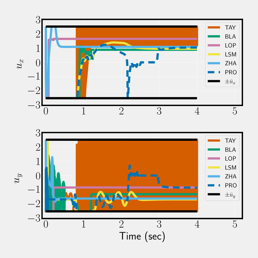
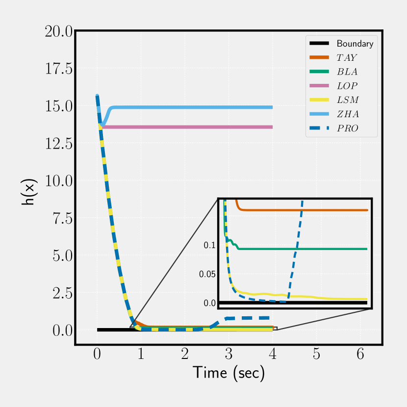
Figure 2: State trajectories, control inputs, and control barrier function evolutions in time for the Shoot the Gap example.

To encode the goal-convergence criterion we define the CLF:

$$V(z)=K_{V}(x^{2}+y^{2}),$$ (37)

The safe states are those residing outside of the two ellipses shown in Figure 1, which results in the following two CBFs:

$$h_{1}(z)=\frac{(x-x_{1})^{2}}{a^{2}}+\frac{(y-y_{1})^{2}}{b^{2}}-1$$ (38)

$$h_{2}(z)=\frac{(x-x_{2})^{2}}{a^{2}}+\frac{(y-y_{2})^{2}}{b^{2}}-1$$ (39)

where $x_{1}$, $x_{2}$, $y_{1}$, $y_{2}$, $a$, and $b$ are parameters that define the location, size, and shape of the ellipses.

We choose the CLF-CBF-QP framework ([10, 7]) for computing the control inputs. While we simulated the controllers from the literature both in their original form and with standardized FxT-CLFs to more fairly assess their abilities, no meaningful differences were observed in their ability to ”shoot the gap.” As such, we present results for the latter case. Our control framework is then:

$$\min_{u,\delta_{0},\delta_{1},...,\delta_{q}}\frac{1}{2}u^{T}Qu +p_{0}\delta_{0}^{2}+\sum_{i=1}^{q}p_{i}\delta_{i}^{2}$$ (40a)

s.t.

$$-\bar{u}_{1}\leq u_{1}\leq\bar{u}_{1}$$ (40b)

$$-\bar{u}_{2}\leq u_{2}\leq\bar{u}_{2}$$ (40c)

$$1 \leq\delta_{i}$$ (40d)

$$L_{f}V(z)+L_{g}V(z)u +\phi(x,\Delta(x,t),\hat{\theta},\eta)$$

$$\leq\delta_{0} -c_{1}V(z)^{\gamma_{1}}-c_{2}V(z)^{\gamma_{2}}$$ (40e)

$$L_{f}h_{i}(z)+L_{g}h_{i}(z)u +\psi(x,\Delta(x,t),\hat{\theta},\eta)\geq-\delta_{i}h_{i}(z)$$ (40f)

$\forall i\in\{1,\ldots,q\}$, where generally $u=[u_{1}\;u_{2}]^{T}$ and for this problem $u_{1}=u_{x}$ and $u_{2}=u_{y}$, $\delta_{0}$ is a relaxation parameter on the performance objective whose inclusion guarantees feasibility of the QP, $\delta_{i}$ allows for larger negative values of $\dot{h}_{i}(z)$ away from the boundary of the safe set, and $p_{i}$ penalizes values of $\delta_{i}$, $\forall i\in\{0,...,q\}$. The functions $\phi:\mathbb{R}^{n}\times\mathbb{R}^{n\times p}\times\mathbb{R}^{p}\times\mathbb{R}^{p}\rightarrow\mathbb{R}$ and $\psi:\mathbb{R}^{n}\times\mathbb{R}^{n\times p}\times\mathbb{R}^{p}\times\mathbb{R}^{p}\rightarrow\mathbb{R}$ represent the terms specific to the way each respective controller handles the uncertainty in the system dynamics. While all of (40b)-(40f) are linear in the decision variables, (40b) and (40c) enforce input constraints, (40d) prevents over-conservatism in enforcing safety, (40e) encodes FxT convergence to the goal, and safety is guaranteed by (40f).

V-A3 Results

The full set of parameters for this numerical case study are provided in Table I.

TABLE I: Shoot the Gap Parameters

$\dot{x}$	Val	QP	Val	CBF	Val	CLF	Val	$\dot{\hat{\theta}}$	Val
$f_{1}$	1	$Q$	$I_{2\times 2}$	$a$	1	$K_{V}$	1	$k_{e}$	0.001
$f_{2}$	4	$p_{0}$	50	$b$	4.99	$T$	4	$T_{e}$	0.2
$\theta_{1}$	-1	$p_{1}$	5	$x_{1}$	1	$\mu$	5	$\mu_{e}$	5
$\theta_{2}$	1	$p_{2}$	5	$x_{2}$	1	$c_{1}$	1.963	$c_{1e}$	50
$\bar{\theta}_{1}$	10	$\bar{u}_{1}$	2.5	$y_{1}$	-6	$c_{2}$	1.963	$c_{2e}$	50
$\bar{\theta}_{2}$	10	$\bar{u}_{2}$	2.5	$y_{2}$	4	$\gamma_{1}$	0.8	$\gamma_{1e}$	0.8
$K_{\Delta}$	0.833					$\gamma_{2}$	1.2	$\gamma_{2e}$	1.2
								$\ell_{e}$	100

We endeavor to demonstrate that by learning the true values of the uncertain parameters in the system dynamics of (36), our method is capable of approaching the boundary of the safe set more closely than previous results in the literature and, as a consequence, able to reach a goal which may require such an approach despite uncertainty. Table II provides the legend codes used to refer to these other works.

TABLE II: Controllers from the Literature

Authors	Citation	Legend Code
Taylor et al.	[11]	TAY
Black et al.	[5]	BLA
Lopez et al.	[12] (w/o SMID)	LOP
Lopez et al.	[12] (w/ SMID)	LSM
Zhao et al.	[14]	ZHA
Proposed Method		PRO

Note: [12] presents RaCBF-based control formulations with and without SMID for parameter estimation. We have considered both cases.

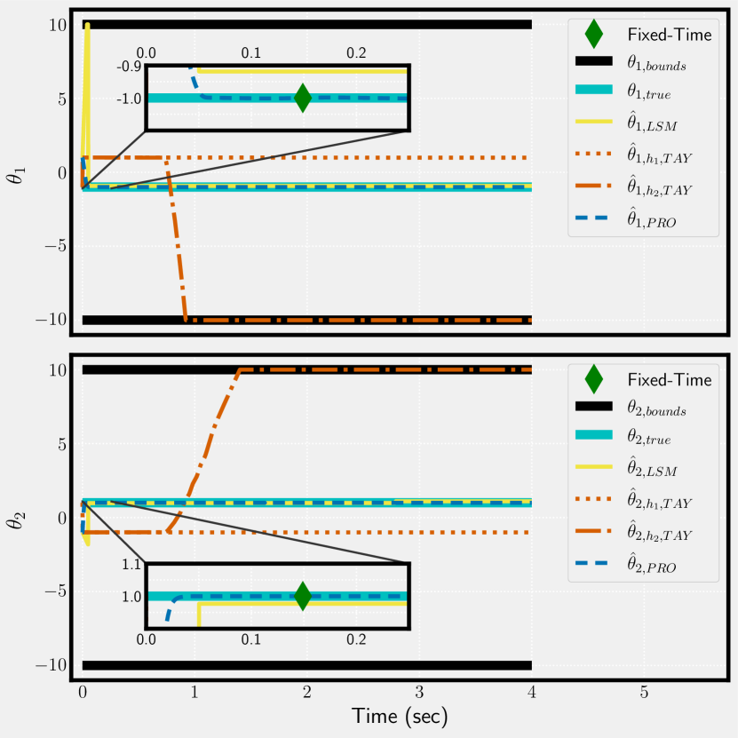
First, we observe that in accordance with Theorem 2, Figure 3 highlights that the parameter estimates, $\hat{\theta}$, do in fact converge to their true values within fixed-time $T_{\theta}$ given by (28).

Figure 3: Estimates of the unknown model parameters, $\theta$.

Figure 2(a) shows that our proposed method ”shoots the gap” where the others do not; that is, our method can tolerate regions of the state space which exist in close proximity to the boundary of the safe region. As such, it fulfills its specification of FxT convergence to the origin. In this sense, our synthesized adaptation law and RaCBF-based controller is less restrictive than the existing literature.

V-B Highway Overtake

We now consider an automobile highway overtake problem, similarly to [5], and show how our control formulation can guarantee success of the overtake maneuver under uncertainty, where the robust CBF approach cannot.

V-B1 Dynamics

Just as in [5], we model the vehicles as kinematic bicycles using the model from [24]. Accordingly, the state vectors are $z_{i}=[x_{i}\;y_{i}\;\theta_{i}\;v_{i}]^{T}$, where $x$ and $y$ are planar Euclidean coordinates (longitudinal and transverse), $\theta$ is the heading angle, $v$ is velocity, and the subscript $i\in\{e,l\}$ denotes belonging to the Ego or Lead vehicle. The corresponding dynamical system is described by:

$$\dot{z}_{i}=\begin{bmatrix}v_{i}\ \cos(\theta_{i})\\ v_{i}\ \sin(\theta_{i})\\ 0\\ 0\end{bmatrix}+\begin{bmatrix}0&0\\ 0&0\\ 1&0\\ 0&1/M\end{bmatrix}\begin{bmatrix}\omega_{i}\\ a_{i}\end{bmatrix}+\Delta_{i}(z)\theta,$$ (41)

where $M$ is the mass of the vehicle in kg, and $\omega_{i}$ and $a_{i}$ represent the angular velocity and heading acceleration control inputs, for which the bounds $\underaccent{\bar}{\omega}\leq\omega_{i}\leq\bar{\omega}$ in rad^-1 and $\underaccent{\bar}{a}\leq a_{i}\leq\bar{a}$ in m/s² hold. For reference, all overtake parameter values may be found in Table III. We elect to model erratic, or distracted, driver behavior by the addition of the uncertain term $\Delta_{i}(x)\theta$, where $\Delta_{i}:\mathbb{R}^{4}\rightarrow\mathbb{R}^{4}\times\mathbb{R}^{2}$ is the known regressor matrix. As such, we let $\Delta_{e}=\bm{0}_{n\times p}$ and $\Delta_{l}=\bm{0}_{n\times p}$ with the exception of $\Delta_{l,(0,0)}(z)=1+\frac{1}{2}(1-\cos(2\pi f_{l,1}x_{l}))$ and $\Delta_{l,(1,1)}(z)=\frac{1}{10}+\frac{1}{20}(1-\sin(2\pi f_{l,2}x_{l}))$.

V-B2 Problem Formulation

We define the safe sets as:

$$S_{i}=\{z\;|\;h_{i}(z)\geq 0\},\;\forall i\in\{1,2,3\}$$ (42)

where

$$h_{1}(z) =K_{s}\left((y_{e}-E_{R}(z))(E_{L}(z)-y_{e})\right)$$ (43)

$$h_{2}(z) =L-v$$ (44)

$$h_{3}(z) =\left(\frac{x_{e}-x_{l}}{s_{x}}\right)^{2}+\left(\frac{y_{e}-y_{l}}{s_{y}}\right)^{2}-1$$ (45)

and

$$E_{R}(z)=e_{r} +\frac{\theta_{e}v_{e}\sin(\theta_{e})}{\bar{\omega}}$$

$$-\frac{\theta_{e}^{2}}{2\bar{\omega}^{2}}\left(\frac{\bar{a}\sin(\theta_{e})}{M}+v_{e}\bar{\omega}\cos(\theta_{e})\right)$$ (46)

$$E_{L}(z)=e_{l} -\frac{\theta_{e}v_{e}\sin(\theta_{e})}{\bar{\omega}}$$

$$-\frac{\theta_{e}^{2}}{2\bar{\omega}^{2}}\left(\frac{\bar{a}\sin(\theta_{e})}{M}-v_{e}\bar{\omega}\cos(\theta_{e})\right)$$ (47)

where $e_{r}$ and $e_{l}$ denote the physical edges of the right and left side of the road such that (46) and (47) imply that (43) encodes that the Ego vehicle remain on the road despite bounded steering control. We also have that (44) enforces the road speed limit, $L$, in m/s, and (45) ensures that safety margins $s_{x}=\tau v_{e}\cos(\theta_{e})+l_{c}$ and $s_{y}=w_{c}+0.75$ between vehicles are observed, where $l_{c}$ and $w_{c}$ are the length and width of the vehicles in m. Then, $S=\cap S_{i}$, $\forall i\in\{1,2,3\}$.

In addition, Oncoming vehicles are known to obey the following pattern: the first vehicle has a time-headway of 24s with the Lead Vehicle, and subsequent Oncoming vehicles arrive in 30s intervals. Consequently, the Ego vehicle must complete the overtake within 24s to proceed at the outset, and within 30s to proceed after the first Oncoming vehicle.

We now formally define the overtake problem.

Problem 2.

Given the initial states, $z_{e}(0)$, $z_{l}(0)$, the time headway of an oncoming vehicle, $T_{h}$, and the set $\Theta$ to which the unknown parameter vector, $\theta$, belongs, determine whether it is safe for the Ego vehicle to overtake the Lead vehicle, i.e. whether there exist $z(t)$, $u_{e}(t)\in\mathcal{U}=\{(\omega_{e},a_{e})\;|\;\underaccent{\bar}{\omega}\leq\omega_{e}\leq\bar{\omega},\;\underaccent{\bar}{a}\leq a_{e}\leq\bar{a}\}$ such that $z_{e}(t)\in S$, $\forall t\in[0,T]$, where $T$ is the upper bound on time to complete the overtake. If safe and $T\leq T_{h}$, design a control input, $u_{e}(t)\in\mathcal{U}$ for the given $z(0)$ such that the Ego vehicle overtakes the Lead vehicle.

V-B3 Control Formulation

Just as in [5], we partition the problem into the following sub-problems:

1. Ego Vehicle approaches Lead Vehicle

2. Ego Vehicle merges into overtake lane

3. Ego Vehicle advances beyond Lead Vehicle

4. Ego Vehicle merges back into original lane

We use the CLF-CBF-QP control framework presented in (40) to compute the control inputs, $u_{1}=\omega_{e}$ and $u_{2}=a_{e}$, pointwise-in-time where $q=3$ in accordance with $h_{1}(z)$, $h_{2}(z)$, and $h_{3}(z)$ in (43)-(45). Our CLF is:

$$V(z)=K_{V}(k_{x}\bar{x}^{2}+k_{y}\bar{y}^{2}+k_{\theta}\bar{\theta}^{2}+k_{v}\bar{v}^{2}-1)$$ (48)

where $\bar{x}=x-x_{d}$, $\bar{y}=y-y_{d}$, $\bar{\theta}=\theta-\theta_{d}$, and $\bar{v}=v-v_{d}$, and $z_{d}=[x_{d}\;y_{d}\;\theta_{d}\;v_{d}]^{T}$ is the desired state. We define the fixed-time convergence times for the four sub-problems as $T_{1}=3$, $T_{2}=5$, $T_{3}=7$, and $T_{4}=5$ respectively.

TABLE III: Overtake Parameters

$\dot{x}$	Val	QP	Val	CBF	Val	CLF	Val	$\dot{\hat{\theta}}$	Val
$M$	1994	$Q_{0,0}$	1/$\bar{\omega}^{2}$	$e_{r}$	0	$K_{V}$	10-5	$k_{e}$	0.001
$f_{l,1}$	0.01	$Q_{1,1}$	1/$\bar{a}^{2}$	$e_{l}$	6	$\mu$	5	$T_{e}$	0.2
$f_{l,2}$	0.02	$p_{0}$	5$\times 10^{8}$	$L$	30	$\gamma_{1}$	0.8	$\mu_{e}$	5
$\theta_{1}$	1	$p_{1}$	1	$l_{c}$	4.81	$\gamma_{2}$	1.2	$c_{1e}$	50
$\theta_{2}$	0	$p_{2}$	1	$w_{c}$	1.92	$k_{x}$	0.0625	$c_{2e}$	50
		$p_{3}$	1	$\tau$	1.8	$k_{y}$	100	$c_{2e}$	50
		$\bar{\omega}$	0.175			$k_{\theta}$	400	$\gamma_{1e}$	0.8
		$\bar{a}$	4890			$k_{v}$	1	$\gamma_{2e}$	1.2
								$\ell_{e}$	100

Note: $Q_{i,j}$ denotes the value of the row $i$ column $j$ entry for the $Q$ matrix. Non-specified entries are uniformly zero.

V-B4 Results

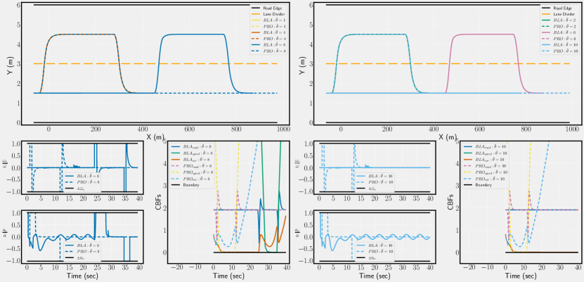
Figure 4: Results for 6 different simulations of the overtake problem. The top row displays state trajectories. The bottom row contains control inputs and CBF trajectories for cases where [5] must postpone the overtake maneuver (left) and cannot complete safely complete it (right).

The scenario was initialized as $x_{e}(0)=-64.8$, $y_{e}(0)=1.5$, $\theta_{e}(0)=0$, $v_{e}(0)=24$, $x_{l}(0)=0$, $y_{l}(0)=1.5$, $y_{\theta}(0)=0$, and $v_{l}(0)=19$. For all considered sets of admissible parameters, $\Theta$, we set $\bar{\theta}=\bar{\theta}_{1}=-\underaccent{\bar}{\theta}_{1}=\bar{\theta}_{2}=-\underaccent{\bar}{\theta}_{2}$, and chose $\bar{\theta}=1,2,4,6,8,10$. Table IV shows how the fixed-time horizon grows for BLA as $\bar{\theta}$ increases.

TABLE IV: Overtake Fixed-Time Horizons

$\bar{\theta}$	$T_{PRO}$	$T_{BLA}$	$t_{oncoming,1}$	$t_{oncoming,i}$
1	20	20.74	24	24 + 30(i-1)
2	20	21.31	24	24 + 30(i-1)
4	20	22.67	24	24 + 30(i-1)
6	20	24.42	24	24 + 30(i-1)
8	20	26.80	24	24 + 30(i-1)
10	20	30.38	24	24 + 30(i-1)

As such, the PRO technique completes the overtake without delay for all parameter bounds, whereas the BLA controller appropriately proceeds immediately with the overtake when $\bar{\theta}=1,2,4$, proceeds after the first oncoming vehicle has passed when $\bar{\theta}=6,8$, and cannot guarantee a safe overtake when $\bar{\theta}=10$. This is precisely the advantage of our proposed controller. Because it is guaranteed to adaptively learn the true parameters within fixed-time, it is able to successfully complete the overtake maneuver for all considered sets, $\Theta$.

VI Conclusion

In this study on the efficacy of various techniques for safe control under parametric model uncertainty, we presented a novel adaptation law that learns the uncertain parameters associated with a class of nonlinear, control-affine dynamical systems in fixed-time. We synthesized our parameter adaptation law with a robust, adaptive CBF-based controller in the form of a quadratic program, and provided an upper bound on the parameter estimation error as an explicit function of time. We then studied the performance of our method on a simple, 2D single integrator system in relation to several recent works from the literature and demonstrated that our contribution succeeds in navigating near unsafe regions where the others fail. We further illustrated the promise of our method in applications where a decision on whether to initiate a possibly unsafe maneuver is required, using the automobile overtake problem as a case study.

In the future, we intend to study cases for which the uncertain parameters are time-varying and an upper bound is not known a priori, as we recognize that these may have broader applicability to real-world scenarios.

References

• [1] P. Wieland and F. Allgöwer, “Constructive safety using control barrier functions,” IFAC Proceedings Vols., vol. 40, no. 12, pp. 462–467, 2007.
• [2] W. S. Cortez, D. Oetomo, C. Manzie, and P. Choong, “Control barrier functions for mechanical systems: Theory and application to robotic grasping,” in IEEE Trans. on Control Systems Tech., 2019, pp. 1–16.
• [3] M. Rauscher, M. Kimmel, and S. Hirche, “Constrained robot control using control barrier functions,” in IEEE/RSJ International Conference on Intelligent Robots and Systems, 2016, pp. 279–285.
• [4] R. Cheng, G. Orosz, R. M. Murray, and J. W. Burdick, “End-to-end safe reinforcement learning through barrier functions for safety-critical continuous control tasks,” Proceedings of the AAAI Conference on Artificial Intelligence, vol. 33, no. 01, pp. 3387–3395, Jul. 2019.
• [5] M. Black, K. Garg, and D. Panagou, “A quadratic program based control synthesis under spatiotemporal constraints and non-vanishing disturbances,” 59th IEEE Conf. on Decision and Control, 2020.
• [6] K. Garg, E. Arabi, and D. Panagou, “Fixed-time control under spatiotemporal and input constraints: A QP based approach,” 2020.
• [7] A. D. Ames, J. W. Grizzle, and P. Tabuada, “Control barrier function based quadratic programs with application to adaptive cruise control,” in 53rd IEEE Conf. on Decision and Control, 2014, pp. 6271–6278.
• [8] A. D. Ames, X. Xu, J. W. Grizzle, and P. Tabuada, “Control barrier function based quadratic programs for safety critical systems,” IEEE Trans. on Automatic Control, vol. 62, no. 8, pp. 3861–3876, 2017.
• [9] A. D. Ames, K. Galloway, K. Sreenath, and J. W. Grizzle, “Rapidly exponentially stabilizing control Lyapunov functions and hybrid zero dynamics,” IEEE Trans. on Automatic Control, vol. 59, no. 4, pp. 876–891, 2014.
• [10] X. Xu, P. Tabuada, J. W. Grizzle, and A. D. Ames, “Robustness of control barrier functions for safety critical control,” IFAC-PapersOnLine, vol. 48, no. 27, pp. 54–61, 2015.
• [11] A. J. Taylor and A. D. Ames, “Adaptive safety with control barrier functions,” in 2020 American Control Conf., 2019, pp. 1399–1405.
• [12] B. T. Lopez, J.-J. E. Slotine, and J. P. How, “Robust adaptive control barrier functions: An adaptive & data-driven approach to safety,” IEEE Control Systems Letters, pp. 1–1, 2020.
• [13] A. J. Taylor, A. Singletary, Y. Yue, and A. D. Ames, “Learning for safety-critical control with control barrier functions,” Proceedings of Machine Learning Research vol, vol. 120, pp. 1–13, 2020.
• [14] P. Zhao, Y. Mao, C. Tao, N. Hovakimyan, and X. Wang, “Adaptive robust quadratic programs using control lyapunov and barrier functions,” 59th IEEE Conf. on Decision and Control, 2020.
• [15] F. Blanchini, “Set invariance in control,” Automatica, vol. 35, no. 11, pp. 1747–1767, 1999.
• [16] S. P. Bhat and D. S. Bernstein, “Finite-time stability of continuous autonomous systems,” SICON, vol. 38, no. 3, pp. 751–766, 2000.
• [17] A. Polyakov, “Nonlinear feedback design for fixed-time stabilization of linear control systems,” IEEE Transactions on Automatic Control, vol. 57, no. 8, p. 2106, 2012.
• [18] M. Bodson, Adaptive control: stability, convergence, and robustness, ser. Prentice Hall advanced reference series.   Prentice Hall, 1989.
• [19] J. Na, G. Herrmann, X. Ren, M. N. Mahyuddin, and P. Barber, “Robust adaptive finite-time parameter estimation and control of nonlinear systems,” IEEE International Symposium on Intelligent Control - Proceedings, pp. 1014–1019, 2011.
• [20] J. Na, M. N. Mahyuddin, G. Herrmann, X. Ren, and P. Barber, “Robust adaptive finite-time parameter estimation and control for robotic systems,” International Journal of Robust and Nonlinear Control, vol. 25, pp. 3045–3071, 11 2015.
• [21] T. Roskilly and R. Mikalsen, Marine systems identification, modeling and control.   Butterworth-Heinemann, 2015.
• [22] Q. Chen, M. Gao, L. Tao, and Y. Nan, “Adaptive fixed time parameter estimation and synchronization control for multiple robotic manipulators,” International Journal of Control, Automation and Systems, vol. 17, pp. 2375–2387, 2019.
• [23] D. G. Luenberger, Optimization by vector space methods, ser. Decision and control.   New York, NY: Wiley, 1969.
• [24] R. Rajamani, Vehicle Dynamics and Control.   Springer US, 2012.