Ultrafast creation and disruption of excitonic condensate in transition metal dichalcogenides revealed by time-resolved ARPES

Transient exciton condensation and its ultrafast disruption in transition metal dichalcogenides revealed by time-resolved ARPES

Ultrafast melting of the nonequilibrium excitonic insulator phase in bulk WeSe₂

Ultrafast creation and melting of nonequilibrium excitonic condensates in bulk WSe₂

Abstract

We study the screened dynamics of the nonequilibrium excitonic consensate forming in a bulk WSe₂ when illuminated by coherent light resonant with the lowest-energy exciton. Intervalley scattering causes electron migration from the optically populated K valley to the conduction band minimum at $\Sigma$. Due to the electron-hole unbalance at the K point a plasma of quasi-free holes develops, which efficiently screens the interaction of the remaining excitons. We show that this plasma screening causes an ultrafast melting of the nonequilibrium consensate and that during melting coherent excitons and quasi-free electron-hole pairs coexist. The time-resolved spectral function does exhibit a conduction and excitonic sidebands of opposite convexity and relative spectral weight that changes in time. Both the dependence of the time-dependent conduction density on the laser intensity and the time-resolved spectral function agree with recent experiments.

I Introduction

Excitons in solids are electron-hole (e-h) bound pairs which behave as composite bosons in the dilute limit Keldysh (1972); Keldysh and Kozlov (1968); Moskalenko and Snoke (2000); Combescot and Shiau (2016). More than three decades ago it was suggested that a nonequilibrium (NEQ) exciton superfluid may form in a semiconductor after pumping with coherent light of frequency smaller than the gap but larger than or at most equal to the exciton energy Schmitt-Rink et al. (1988); Kuklinski and Mukamel (1990); Glutsch and Zimmermann (1992); Littlewood and Zhu (1996). The pump would then drive the system from a non-generate ground-state (insulating phase) to a symmetry-broken excited state known as the NEQ excitonic insulator (EI) Östreich and Schönhammer (1993); Hannewald et al. (2000); Glutsch et al. (1992); Perfetto et al. (2019). It has been recently shown that the NEQ-EI state emerges also from the spontaneous symmetry breaking of a macroscopically degenerate excited manifold Perfetto et al. (2019); Szymańska et al. (2006); Hanai et al. (2016, 2017); Triola et al. (2017); Hanai et al. (2018); Pertsova and Balatsky (2018); Becker et al. (2019); Yamaguchi et al. (2013); Pertsova and Balatsky (2020).

In time-resolved (tr) ARPES the NEQ-EI phase generates a replica of the valence band at the exciton energy, i.e. below the conduction band minimum (CBM) Schmitt-Rink et al. (1988); Perfetto et al. (2019); Christiansen et al. (2019); Perfetto et al. (2020a). The experimental observation of this excitonic sideband is usually challenging Madéo et al. (2020); Lee et al. (2020) since excitons may quickly loose coherence Koch et al. (2006) due to electron-phonon scattering Madrid et al. (2009); Nie et al. (2014); Selig et al. (2016); Sangalli et al. (2018) or break due to excited-state screening mechanisms Chernikov et al. (2015a, b); Cunningham et al. (2017); Yao et al. (2017); Wang et al. (2019); Dendzik et al. (2020). As a result the ARPES signal changes rapidly with increasing pump-probe delay Perfetto et al. (2016); Steinhoff et al. (2017); Rustagi and Kemper (2018); Christiansen et al. (2019); Perfetto et al. (2020a) and the measured spectra become difficult to interpret. The development of a microscopic theory which takes into account decoherence, screening and other material-specific properties is necessary in order to understand the ultrafast dynamics and interpret the experimental results.

In this work we put forward a microscopic theory for bulk WSe₂, an indirect gap semiconductor Jiang (2012) with an optically bright exciton of energy slightly above the gap Beal and Liang (1976); Finteis et al. (1997); Arora et al. (2015); Riley et al. (2015); Kim et al. (2016). A distinct physical picture emerges from our calculations, see Fig. 1. The pump-induced photoexcitation initially generates an exciton superfluid around the K point Frindt (1963); Wang et al. (2018). Due to intervalley scattering Bertoni et al. (2016), however, electrons migrate from the K-valley to the CBM at the $\Sigma$-valley Jiang (2012), and excitons begin to dissociate. Consequently, a gas of free holes, i.e., holes not bounded to conduction electrons, forms in the valence band at the K-point. This hole-plasma efficiently screens Steinhoff et al. (2014); Liang and Yang (2015); Meckbach et al. (2018) the electron-hole attraction and eventually causes an ultrafast melting of the remaining excitons Dendzik et al. (2020). During the melting process the quasi-free e-h pairs coexist with excitons in the NEQ-EI phase.

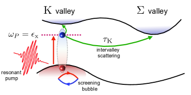
Figure 1: The NEQ-EI state is created in the K valley, where bright excitons are initially photo-excited. Subsequent $\mathrm{K}\to\Sigma$ intervalley scattering of excited carriers breaks charge neutrality in the K valley, and free K-valence holes screen the Coulomb repulsion. The reduction of e-h attraction causes exciton breaking, and free electrons occupy the available conduction states in the K valley.

Through real-time simulations and self-consistent excited-state calculations we show the formation of the NEQ-EI phase during resonant pumping as well as its fingerprints in tr-ARPES spectra. If screening is neglected then the excitonic sideband is simply attenuated by the K$\to\Sigma$ intervalley scattering as the pump-probe delay increases. If, instead, both screening and intervalley scattering are taken into account then the instantaneous formation of the excitonic sideband is followed by the development of a quasiparticle sideband, signaling the coexistence of quasi-free e-h pairs and excitons. The spectral weight is then rapidly transferred from the excitonic sideband to the quasiparticle sideband until the extinction of the former. The calculated tr-ARPES spectra of bulk $\mathrm{WSe}_{2}$ agrees well with recent experiments on the same system Puppin (2018) if the K$\to\Sigma$ scattering rate is estimated to be $\approx 15$ fs Bertoni et al. (2016); Dendzik et al. (2020); Puppin (2018). Our simulations indicate that in this case the NEQ-EI phase melt in few tens of femtoseconds. Although the interplay of intervalley scattering and enhanced screening is investigated in bulk $\mathrm{WSe}_{2}$ the highlighted mechanism is general and it is likely to occur in other indirect gap semiconductors.

The paper is organized as follows. In the next Section we present our microscopic modelling of bulk $\mathrm{WSe}_{2}$. We illustrate the equation of motion for the one-particle density matrix that accounts for coherent exciton formation in the K valley upon optical excitation, for the subsequent K$\to\Sigma$ intervalley scattering of excited carriers, and for the plasma-induced screening. In Section III we discuss the Floquet solution of the equation of motion, useful for characterizing the transient NEQ-EI state at the K point forming after resonant pumping. Real-time simulations of WSe₂ driven by a VIS pulse of duration $\simeq 10^{2}$ fs are introduced in Section IV. In Section V we present results in the absence of plasma screening. We show that in this case the time-dependent solution follows adiabatically the Floquet solution and that exciton dissociation induced by intervalley scattering does not destroy the NEQ-EI phase. In Section VI both intervalley scattering and screening effects are taken into account. Through tr-ARPES spectra we show that the initial NEQ-EI phase is slowly contaminated by quasi-free e-h pairs until an incoherent plasma of electrons and holes is formed. A summary of the main findings are drawn in Section VII.

II Microscopic Theory

Bulk $\mathrm{WSe}_{2}$ is an indirect-gap semiconductor Jiang (2012) with the property that optical excitations of frequency close or below the gap create e-h pairs around the K and K’ points Frindt (1963); Wang et al. (2018), where the direct gap is located Jiang (2012). The two-dimensional (2D) character of the valence and conduction band close to the K points Bertoni et al. (2016) allows for modelling the e-h dynamics using a 2D two-band model. In the following we neglect the spin-orbit coupling and consider degenerate and decoupled K and K’ valleys. The inclusion of the spin-orbit coupling does not change the main conclusions. Let $\epsilon_{v{\mathbf{k}}}$ and $\epsilon_{c{\mathbf{k}}}$ be the valence and conduction dispersion and $\epsilon_{g}\equiv\mathrm{min}[\epsilon_{c{\mathbf{k}}}]-\mathrm{max}[\epsilon_{v{\mathbf{k}}}]=1.8$ eV Jiang (2012); Beal and Liang (1976); Finteis et al. (1997); Arora et al. (2015); Riley et al. (2015); Kim et al. (2016) define the direct gap. Placing the K point at ${\mathbf{k}}=0$ we use quadratic dispersions $\epsilon_{v{\mathbf{k}}}=-\frac{k^{2}}{2m}-\frac{\epsilon_{g}}{2}$ and $\epsilon_{c{\mathbf{k}}}=\frac{k^{2}}{2m}+\frac{\epsilon_{g}}{2}$, with $k=|{\mathbf{k}}|$. We parametrize the electron-hole attraction according to Ref. Steinhoff et al. (2017)

$$U_{{\mathbf{q}}}=\frac{v_{{\mathbf{q}}}}{\epsilon_{{\mathbf{q}}}},$$ (1)

where

$$v_{{\mathbf{q}}} =\frac{2\pi}{q(1+\gamma q+\delta q^{2})}$$ (2)

is the bare interaction and

$$\epsilon_{{\mathbf{q}}} =\epsilon^{\infty}_{{\mathbf{q}}}\frac{1-\beta_{1{\mathbf{q}}}\beta_{2{\mathbf{q}}}e^{-2hq}}{1+(\beta_{1{\mathbf{q}}}+\beta_{2{\mathbf{q}}})e^{-hq}+\beta_{1{\mathbf{q}}}\beta_{2{\mathbf{q}}}e^{-2hq}}$$ (3)

accounts for the screening. In Eq. (3)

$$\epsilon^{\infty}_{{\mathbf{q}}} =g+\frac{a+q^{2}}{\frac{a\sin(qc)}{qbc}+q^{2}}$$ (4)

is the dielectric function of the neglected bands whereas

$$\beta_{i{\mathbf{q}}} =\frac{\epsilon^{\infty}_{{\mathbf{q}}}-\epsilon_{\mathrm{sub,i}}}{\epsilon^{\infty}_{{\mathbf{q}}}+\epsilon_{\mathrm{sub,i}}}$$ (5)

takes into account the dielectric constant $\epsilon_{\mathrm{sub,i}}$ of a possible substrate ($i=1$) or superstrate ($i=2$). Realistic parameters to describe a single layer of $\mathrm{WSe}_{2}$ close to the K point are Steinhoff et al. (2017) $m/m_{e}=0.34$ (where $m_{e}$ is the free electron mass), $a=2.4~{}\mathring{\mathrm{A}}^{-2}$, $b=21$, $c=5.7~{}\mathring{\mathrm{A}}$, $h=2.5~{}\mathring{\mathrm{A}}$, $g=5.3$, $\gamma=2.3~{}\mathring{\mathrm{A}}$, $\delta=0.174~{}\mathring{\mathrm{A}}^{2}$. Top and bottom layers play the role of a superstrate and substrate respectively Latini et al. (2015); therefore $\epsilon_{\mathrm{sub,1}}=\epsilon_{\mathrm{sub,2}}\equiv\epsilon$. The value $\epsilon=6$ is chosen to reproduce the lowest (bright) A-exciton of energy $\epsilon_{\rm x}=1.7$ eV (binding energy $\epsilon_{b}=\epsilon_{g}-\epsilon_{\rm x}=0.1~{}\mathrm{eV}$), in agreement with the literature Beal and Liang (1976).

We are interested in the electronic properties of $\mathrm{WSe}_{2}$ under weak resonant pumping – hence with a photon frequency equal to the lowest bright exciton energy. As we shall see the injected exciton fluid inherits the coherence of the laser pulse and a NEQ-EI phase is transiently generated. Pump-probe experiments Wallauer et al. (2016); Bertoni et al. (2016); Waldecker et al. (2017); Madéo et al. (2020) have provided evidence that excited carriers experience a fast intervalley scattering due to electron-electron Haug et al. (1994); Steinhoff et al. (2016); Schmidt et al. (2016) and electron-phonon interactions Selig et al. (2016); Molina-Sánchez et al. (2017). The intervalley scattering transfers the pumped electrons from the K valley to the CBM at the $\Sigma$ valley on a time-scale $\tau_{\mathrm{K}}\approx 15$ fs Puppin (2018). After the K$\to\Sigma$ scattering electrons escape from the considered layer since the valence band at the $\Sigma$ point has a three-dimensional character Bertoni et al. (2016). The lickage of conduction electron from the K point is taken into account by adding a drain term to the equation of motion for the density matrix, see below.

Intervalley scattering has also a pivotal role in renormalizing the effective e-h attraction. Indeed the total conduction density $n_{\rm e}(t)$ (i.e. the sum of K and K’ valleys contributions) becomes smaller than the corresponding valence hole-density $n_{\rm h}(t)$. This gives rise to a finite density $n_{\mathrm{pl}}=(n_{\mathrm{h}}-n_{\rm e})/2$ of free holes in each K valley. Under the weak pumping assumption the screening due to excitons is negligible and can be discarded Perfetto et al. (2020b). Thus the screened e-h interaction $W_{{\mathbf{q}}}$ is given by

$$W_{{\mathbf{q}}}=\frac{U_{{\mathbf{q}}}}{1-2U_{{\mathbf{q}}}\chi_{{\mathbf{q}}}^{\mathrm{pl}}},$$ (6)

where $\chi_{{\mathbf{q}}}^{\mathrm{pl}}$ is 2D Lindhard function Giuliani and Vignale (2005)

$$\chi_{{\mathbf{q}}}^{\mathrm{pl}}=\frac{m}{\pi}\left[\theta(q-\sqrt{8\pi n_{\mathrm{pl}}})\sqrt{1-\frac{8\pi n_{\mathrm{pl}}}{q^{2}}}-1\right].$$ (7)

With this premise, the equation of motion for the $2\times 2$ one-particle density matrix in the Hartree plus Screened Exchange (HSEX) approximation reads

$$-i\frac{d}{dt}\rho_{{\mathbf{k}}}(t)+[h_{\mathrm{HSEX},{\mathbf{k}}}(t),\rho_{{\mathbf{k}}}(t)]-\frac{i}{2}\{\Gamma,\rho_{{\mathbf{k}}}(t)\}=0,$$ (8)

where the $2\times 2$ matrix of the drain term

$$\Gamma=\left(\begin{array}[]{cc}0&0\\ 0&\tau^{-1}_{\mathrm{K}}\\ \end{array}\right)$$ (9)

accounts for intervalley scattering and it ensures an exponential depletion of the conduction density on the $\tau_{\mathrm{K}}$ time-scale. The time-dependent HSEX hamiltonian in the presence of an electric field $E(t)$ coupled to the valence-conduction dipole moments $d_{{\mathbf{k}}}$ reads

$$h_{\mathrm{HSEX},{\mathbf{k}}}(t)=\left(\begin{array}[]{cc}\epsilon_{v{\mathbf{k}}}+V^{vv}_{{\mathbf{k}}}(t)&V^{vc}_{{\mathbf{k}}}(t)+E(t)d_{{\mathbf{k}}}\\ V^{cv}_{{\mathbf{k}}}(t)+E(t)d_{{\mathbf{k}}}&\epsilon_{c{\mathbf{k}}}+V^{cc}_{{\mathbf{k}}}(t)\\ \end{array}\right)$$ (10)

with HSEX potential

$$V^{vv}_{{\mathbf{k}}}(t) =-\frac{1}{\mbox{$\mathcal{N}$}}\sum_{{\mathbf{q}}}W_{{\mathbf{k}}-{\mathbf{q}}}(t)[\rho^{vv}_{{\mathbf{q}}}(t)-1]$$ (11a)

$$V^{cc}_{{\mathbf{k}}}(t) =-\frac{1}{\mbox{$\mathcal{N}$}}\sum_{{\mathbf{q}}}W_{{\mathbf{k}}-{\mathbf{q}}}(t)\rho^{cc}_{{\mathbf{q}}}(t)$$ (11b)

$$V^{cv}_{{\mathbf{k}}}(t) =V^{vc*}_{{\mathbf{k}}}(t)=-\frac{1}{\mbox{$\mathcal{N}$}}\sum_{{\mathbf{q}}}W_{{\mathbf{k}}-{\mathbf{q}}}(t)\rho^{vc}_{{\mathbf{q}}}(t).$$ (11c)

We emphasize that the HSEX potential depends on the density matrix explicitly as well as implicitly through the dependence of $W$ on $n_{\mathrm{pl}}=(n_{\rm h}-n_{\rm e})/2$. The density of conduction electron and valence holes is indeed given by $n_{\rm e}(t)=\frac{4}{\mathcal{NA}}\sum_{{\mathbf{k}}}\rho^{cc}_{{\mathbf{k}}}(t)$ and $n_{\rm h}(t)=\frac{4}{\mathcal{NA}}\sum_{{\mathbf{k}}}(1-\rho^{vv}_{{\mathbf{k}}}(t))$, where $\mathcal{N}$ is the number of ${\mathbf{k}}$-points and $\mathcal{A}=9.53\times 10^{-16}$ cm² is the area of the unit cell of a $\mathrm{WSe}_{2}$ layer. Here the factor 4 in front of $n_{\rm e}$ and $n_{\rm h}$ accounts for the spin and valley degeneracy.

Below we solve numerically Eq. (8) using the ground-state density matrix $\rho_{g,{\mathbf{k}}}=\left(\begin{array}[]{cc}1&0\\ 0&0\end{array}\right)$ as initial condition. However, in order to shed light on the nature of the time-dependent results we preliminary discuss the Floquet solution of Eq. (8) at zero electric field.

III NEQ-EI phase from the Floquet solution

The Bose-Einstein condensation of excitons in equilibrium matter is predicted in narrow-gap semiconductors or semimetals where the exciton binding energy is larger than the bandgap Halperin and Rice (1968); Blatt et al. (1962); Keldysh and Kopaev (1965); Kozlov and Maksimov (1965); Jérome et al. (1967); Keldysh and Kozlov (1968); Comte, C. and Nozières, P. (1982). In this case the system is unstable toward the spontaneous formation of excitons, leading to a symmetry-broken state called excitonic insulator (EI). The mean-field theory of EIs has a close analogy to the BCS theory and the resulting exciton superfluid is characterized by a nonvanishing order parameter $\rho^{cv}_{{\mathbf{k}}}$. In a NEQ-EI the symmetry breaking is induced by the pump field Schmitt-Rink et al. (1988). However, we have recently shown that the NEQ-EI phase can also be obtained by solving a BCS-like problem with different chemical potentials $\mu_{v}$ and $\mu_{c}$ for valence and conduction electrons Perfetto et al. (2019). Below we briefly revisit this excited-state self-consistent approach and provide a characterization of the solution. As we are interested in describing a stable NEQ-EI we discard the intervalley scattering for the time being.

In the HSEX approximation the lowest-energy density matrix corresponding to a quantum state with a finite density of conduction electrons and valence holes can be written as Perfetto et al. (2019); Perfetto et al. (2020b)

$$\rho^{\alpha\beta}_{{\mathbf{k}}}=\sum_{\xi}f(e^{\xi}_{{\mathbf{k}}})\varphi^{\xi}_{\alpha{\mathbf{k}}}\varphi^{\xi\ast}_{\beta{\mathbf{k}}}.$$ (12)

In Eq. (12) $f(x)=1/(e^{x/T}+1)$ is the Fermi function at temperature $T$ and the two-dimensional vector $\varphi^{\xi}_{{\mathbf{k}}}$ solves the secular problem

$$\big{(}h_{\rm HSEX,{\mathbf{k}}}-\mu\big{)}\varphi^{\xi}_{{\mathbf{k}}}=e^{\xi}_{{\mathbf{k}}}\varphi^{\xi}_{{\mathbf{k}}},$$ (13)

where $\xi=\pm$ labels the two eigenvectors and

$$\mu=\left(\!\!\begin{array}[]{cc}\mu_{v}&0\\ 0&\mu_{c}\\ \end{array}\!\!\right)\!\!$$ (16)

is the matrix of chemical potentials ensuring that both $n_{\rm e}$ and $n_{\rm h}$ are nonvanishing. The secular problem must be solved self-consistently since the HSEX potential is a functional of $\rho$. The symmetry of the problem ensures that $e^{-}_{{\mathbf{k}}}<0<e^{+}_{{\mathbf{k}}}$, hence charge neutral solutions $n_{\rm e}=n_{\rm h}$ are obtained for $\mu_{v}=-\mu_{c}$. In the reminder of this work we work at zero temperature and therefore $\rho^{\alpha\beta}_{{\mathbf{k}}}=\varphi^{-}_{\alpha{\mathbf{k}}}\varphi^{-\ast}_{\beta{\mathbf{k}}}$. The ground state solution $\rho=\rho_{g}$ is recovered for $\mu_{v}=\mu_{c}=0$, as it should.

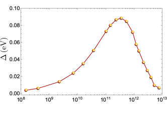
Figure 2: Order parameter $\Delta$ versus electronic density $n_{\rm e}$. The inset shows the spectral function in Eq. (24) for $n_{\mathrm{e}}=1.6\times 10^{10}\mathrm{cm}^{-2}$. The excitonic sideband has been magnified by a factor 10 for a better visualization. Energies are measured with respect to the maximum of the valence band (VBM). Horizontal dashed lines at $\omega=\epsilon_{g}$ and $\omega=\epsilon_{\mathrm{\rm x}}$ are also drawn.

A symmetry broken NEQ-EI solution exists if the difference between the chemical potentials is larger than the lowest exciton energy $\epsilon_{\mathrm{\rm x}}$, i.e., $\delta\mu\equiv\mu_{c}-\mu_{v}>\epsilon_{\mathrm{\rm x}}$ Perfetto et al. (2019). The NEQ-EI solution is characterized by a finite $\rho_{{\mathbf{k}}}^{cv}$ and an infinite degeneracy since if $\varphi^{\xi}_{{\mathbf{k}}}=\left(\begin{array}[]{c}\varphi^{\xi}_{v{\mathbf{k}}}\\ \varphi^{\xi}_{c{\mathbf{k}}}\end{array}\right)$ is a solution then $\varphi^{\xi}_{{\mathbf{k}}}(\theta)=\left(\begin{array}[]{c}\varphi^{\xi}_{v{\mathbf{k}}}\\ e^{i\theta}\varphi^{\xi}_{c{\mathbf{k}}}\end{array}\right)$ is a solution too. To quantify the magnitude of the symmetry breaking we choose the order parameter to be the HSEX potential in Eq. (11c) calculated at ${\mathbf{k}}=0$ and with real vectors $\varphi^{\xi}_{{\mathbf{k}}}$

$$\Delta\equiv V^{cv}_{{\mathbf{k}}=0}=-\frac{1}{\mbox{$\mathcal{N}$}}\sum_{{\mathbf{q}}}W_{{\mathbf{q}}}\varphi^{-}_{c{\mathbf{q}}}\varphi^{-}_{v{\mathbf{q}}}.$$ (17)

In Fig. 2 we show the values of $\Delta$ for the two-band model of $\mathrm{WSe}_{2}$. The order parameter is nonvanishing up to high densities $n_{\rm e}\sim 10^{13}\mathrm{cm}^{-2}$, and it reaches its maximum value for $n_{\rm e}\sim 5\times 10^{11}\mathrm{cm}^{-2}$. We observe that in this calculation $n_{\rm pl}=0$ since no intervalley scattering is included. Hence $W_{{\mathbf{q}}}=U_{{\mathbf{q}}}$ coincides with the bare interaction, in agreement with recent findings on excitonic screening, see Ref. Perfetto et al. (2020b) and Appendix A.

Useful insight on the self-consistent solution comes from the low-density limit, i.e., $\delta\mu\gtrsim\epsilon_{\rm x}$. It can be shown Perfetto et al. (2019) that in this case

$$e^{-}_{{\mathbf{k}}}\approx\epsilon_{v{\mathbf{k}}}+\delta\mu/2,$$ (18)

with

$$\left(\begin{array}[]{c}\varphi^{-}_{v{\mathbf{k}}}\\ \varphi^{-}_{c{\mathbf{k}}}\end{array}\right)\simeq\left(\begin{array}[]{c}1\\ \sqrt{(N_{\rm e}/2)}\,Y_{{\mathbf{k}}}\end{array}\right).$$ (19)

In Eq. (19) the quantity $N_{\rm e}=\frac{1}{2}\mbox{$\mathcal{N}$}\mbox{$\mathcal{A}$}\,n_{\rm e}$ is the number of conduction electrons per valley whereas $Y_{{\mathbf{k}}}$ is the normalized, i.e., $\sum_{{\mathbf{k}}}|Y_{{\mathbf{k}}}|^{2}=1$, lowest-energy solution of the Bethe-Salpeter equation

$$(\epsilon_{c{\mathbf{k}}}-\epsilon_{v{\mathbf{k}}}-\epsilon_{\rm x})Y_{{\mathbf{k}}}=\frac{1}{\mathcal{N}}\sum_{{\mathbf{q}}}U_{{\mathbf{k}}-{\mathbf{q}}}Y_{{\mathbf{q}}}.$$ (20)

Defining the creation operator for the (zero-momentum) exciton according to $\hat{b}^{{\dagger}}=\sum_{{\mathbf{k}}\sigma}Y_{{\mathbf{k}}}\hat{c}^{{\dagger}}_{{\mathbf{k}}\sigma}\hat{v}_{{\mathbf{k}}\sigma}$ we show in Appendix B that total number of excitons $N_{\mathrm{ex}}\equiv\langle\hat{b}^{{\dagger}}\hat{b}\rangle$ is the same as $N_{\rm e}$, i.e.,

$$N_{\mathrm{ex}}=N_{\rm e}.$$ (21)

Thus in the dilute limit all e-h pairs participate to the creation of excitons and these excitons condense in the lowest energy state, consistently with the BEC picture.

The most remarkable feature of the NEQ-EI phase is that the corresponding quantum state is not a stationary state. In fact, using the NEQ-EI density matrix as initial condition one finds that the equation of motion (8) (with $\Gamma=0$) at zero external field, i.e., $E(t)=0$, is satisfied by

$$\rho_{{\mathbf{k}}}(t)=\left(\begin{array}[]{cc}\rho_{{\mathbf{k}}}^{vv}&\rho^{vc}_{{\mathbf{k}}}e^{-i\delta\mu t}\\ \rho^{cv}_{{\mathbf{k}}}e^{i\delta\mu t}&\rho_{{\mathbf{k}}}^{cc}\end{array}\right),$$ (22)

implying that the order parameter evolves in time according to Östreich and Schönhammer (1993); Szymańska et al. (2006); Perfetto et al. (2019)

$$\Delta(t)=\Delta e^{-i\delta\mu t}.$$ (23)

These self-sustained oscillations generate a Floquet-like regime Perfetto and Stefanucci (2020) in the absence of external driving which is expected to survive over a timescale dictated by the exciton lifetime. Striking features of the NEQ-EI phase have been predicted in relation to time-resolved (tr) ARPES experiments Perfetto et al. (2020a). For long enough probes the excitonic condensate generates a replica of the valence band at the exciton energy. Reducing the probe duration below the condensate period $T_{\rm NEQ-EI}\equiv 2\pi/\delta\mu$ the replica fades away and the ARPES signal becomes periodic with period $T_{\rm NEQ-EI}$. The observation of the latter effect is experimentally challenging. However, distinguishing the excitonic replica is within reach of modern ARPES techniques provided that the exciton life-time is longer than the inverse of the exciton energy. The ARPES signal is in this case proportional to the spectral function which is in turn given by Perfetto et al. (2019)

$$A_{{\mathbf{k}}}(\omega)=|\varphi^{-}_{v{\mathbf{k}}}|^{2}\delta(\omega-e^{-}_{{\mathbf{k}}}+\frac{\delta\mu}{2})+|\varphi^{-}_{c{\mathbf{k}}}|^{2}\delta(\omega-e^{-}_{{\mathbf{k}}}-\frac{\delta\mu}{2}).$$ (24)

In the dilute limit $e^{-}_{{\mathbf{k}}}\approx\epsilon_{v{\mathbf{k}}}+\delta\mu/2$, see Eq. (18), and therefore a replica of the valence band (shifted upward by $\epsilon_{\rm x}$) appears inside the gap, see inset of Fig. 2. Interestingly, the spectral weight of the excitonic sideband is proportional to the ${\mathbf{k}}$-resolved conduction density $|\varphi^{-}_{c{\mathbf{k}}}|^{2}$ which, according to Eq. (19), is proportional to the square of the excitonic wavefunction.

In the following we show that the NEQ-EI phase discussed in this Section can be generated in real-time by driving the system with laser pulses of proper subgap frequency. The inclusion of intervalley scattering and screening, however, affect the stability of the photoinduced exciton superfluid with inevitable and interesting repercussions on the time-dependence of the spectral function.

IV Real-time simulations

We investigate the non-equilibrium electronic properties of $\mathrm{WSe}_{2}$ under weak pumping resonant with the lowest bright exciton energy. As resonant photoexcitation provides an efficient injection of excitons, we expect that the NEQ-EI phase can be reached during the time evolution. Indeed, the external radiation transfers coherence to the e-h liquid which can then condense in an exciton superfluid.

In our simulations the system is photoexcited by a VIS pulse of finite duration $T_{P}$, maximum intensity $E_{P}$ and centered around the frequency $\omega_{P}$:

$$E(t)=\theta(1-|1-2t/T_{P}|)E_{P}\sin^{2}(\frac{\pi t}{T_{P}})\sin(\omega_{P}t),$$ (25)

To display our numerical results it is convenient to set the origin of times at $T_{P}/2$ (pump peak). This choice is inspired by the experimental convention to set the origin of delays $\tau$ when the temporal distance between the pump and probe peaks vanishes. Notice that this convention allows for a a direct comparison with esperimental data since the calculated conduction density $n_{\rm e}(\tau)$ at time $\tau$ is proportional to the tr-ARPES spectral weight relative to the conduction band observed at delay $\tau$. We assume momentum-independent dipole moments $d_{{\mathbf{k}}}=d$ and define the Rabi frequency, which determines the strength of the light-matter coupling, as $\Omega_{P}=E_{P}d$. The simulations have been performed with the CHEERS code Perfetto and Stefanucci (2018) using a weak pump, $\Omega_{P}=13$ meV, of duration $T_{P}=100$ fs (FWHM = 50 fs) and resonant frequency $\omega_{P}=\epsilon_{\rm x}=1.7$ eV. According to our convention the initial time is then $t=-50$ fs.

We calculate the density of conduction electrons $n_{\rm e}(t)$ and valence holes $n_{\rm h}(t)$ as well as the time-dependent order parameter $\Delta(t)=-\frac{1}{\mathcal{N}}\sum_{{\mathbf{q}}}W_{{\mathbf{q}}}\rho^{vc}_{{\mathbf{q}}}(t)$. We also calculate the time-dependent spectral function $A_{{\mathbf{k}}}(\tau,\omega)$ at time $\tau$. As discussed in Ref. Perfetto et al. (2020a) this quantity is proportional to the tr-ARPES spectrum measured by a EUV probe at delay $\tau$. In our simulations we have used a probing temporal window of 70 fs, see also Appendix C.

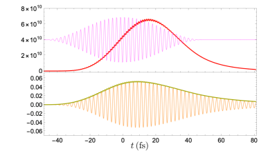
Figure 3: Evolution of the conduction density $n_{\rm e}(t)$ at the K point (panel a) and order parameter $\Delta(t)$ (panel b) without screening effects. The profile of the pump field is displayed in panel a (magenta curve).

V Unscreened dynamics: Robustness of the NEQ-EI phase

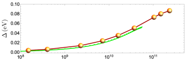
Figure 4: Comparison between the self-consistent pairs $\{n_{\rm e},\Delta\}$ of Fig. (2) (yellow bullets) and the time-dependent pairs $\{n_{\rm e}(t),\Delta(t)\}$ of Fig. 3 (green curve).

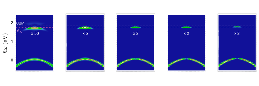
Figure 5: Transient spectral function $A_{{\mathbf{k}}}(\tau,\omega)$ evaluated without screening effects at different delays. The intensity from the conduction band is multiplied by the factor $M=2S_{v}/S_{c}$ where $S_{\alpha}$ is the spectral weight of band $\alpha=v,c$ at ${\mathbf{k}}=0$. Energies are measured with respect to the the valence band maximum. Horizontal dashed lines at energies $\epsilon_{g}$ (white) and $\epsilon_{\mathrm{\rm x}}$ (red) are drawn to guide the eye.

We first investigate the effects of intervalley scattering by neglecting screening effects, i.e., we propagate Eq. (8) by setting $W_{{\mathbf{q}}}(t)=U_{{\mathbf{q}}}$. In Fig. 3 we plot the evolution of the excited density $n_{\rm e}(t)$ (panel a) and order parameter $\Delta(t)$ (panel b) during and after pumping. We see that $n_{\rm e}(t)$ reaches a maximum value about $20$ fs after the pump peak, and then it decays exponentially on the time-scale $\tau_{\mathrm{K}}=15$ fs. The intervalley scattering is also responsible for an exponential decay of the amplitude of the order parameter $\Delta(t)$ on the time-scale $\sim 2\tau_{\mathrm{K}}$. However, coherence is preserved since the order parameter continues to oscillate monochromatically.

In Fig. 4 we show the points $\{n_{\rm e},\Delta\}$ belonging to self-consistent solution of Fig. 2 together with the parametric plot of the points $\{n_{\rm e}(t),|\Delta(t)|\}$ belonging to the temporal evolution of Fig. 3. For times $t\lesssim 20$ fs, i.e., before the conduction density $n_{\rm e}(t)$ reaches its maximum value, the system visits instantaneously all NEQ-EI states of the self-consistent solution. This “adiabatic” behaviour is a consequence of the resonant pumping. Indeed a weak photoexcitation can only create coherent excitons if $\omega_{P}=\epsilon_{\rm x}<\epsilon_{g}$ (quasi-particle states are accessible only for $\omega_{P}>\epsilon_{g}$) and therefore $N_{\mathrm{ex}}(t)=N_{\mathrm{e}}(t)$, see Eq. (21).

Due to the intervalley scattering the spectral function becomes time-dependent. In Fig. 5 we show $A_{{\mathbf{k}}}(\tau,\omega)$ for different times $\tau$. As expected, for small delays $A_{{\mathbf{k}}}(\tau,\omega)$ displays the typical excitonic sideband inside the gap, lying exactly $\epsilon_{b}=0.1$ eV below the CBM. This further corroborates the adiabatic scenario according to which the NEQ-EI state is generated during pumping, see inset of Fig. 2. More importantly, the excitonic sideband survives also at larger delays. This implies that conduction electrons at K remain bound and excitons do not break into free e-h pair at K but only into free electrons at $\Sigma$ and free holes at K. We conclude that an uncontaminated NEQ-EI phase, or equivalently a BEC state of coherent excitons, exists until all excitons break.

VI Screened Dynamics: Ultrafast melting of the NEQ-EI phase

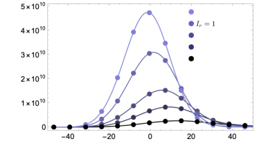
Figure 6: Temporal evolution of the excited density $n_{\mathrm{e}}(t)$ for different pump intensities $I_{r}$ in the TD-HSEX approximation.

In this Section we discuss how the dynamics changes when screening is included. Before, however, we assess the validity of the time-dependent plasma screening approximation in Eqs. (6) and (7). To this end we study how $n_{\rm e}(t)$ varies as the intensity of the pump field increases. This issue has been experimentally investigated in Ref. Puppin (2018) and it has been found that the time at which $n_{\rm e}(t)$ is maximum approaches zero with increasing intensity. In Fig. 6 we show $n_{\rm e}(t)$ for different relative intensities $I_{r}=(\Omega_{P}/\Omega_{0})^{2}$, with $\Omega_{0}=13$ meV. The experimental trend is fairly reproduced. We emphasize that the screened dynamics is crucial for this agreement. In fact, simulations performed with unscreened interaction reveal that the of maximum of $n_{\rm e}(t)$ is independent of the pump intensity (not shown) .

In Fig. 7 we show again the conduction density and the order parameter when both intevalley scattering and screening are taken into account. The pump pulse is the same as in Fig. 3. The maximum value of $n_{\rm e}(t)$ is twice smaller than in the unscreened dynamics and it occurs at time $t\approx 0$, i.e., when the pump pulse is maximum. After this time electrons rapidly migrate to the $\Sigma$ valley and at $t\approx 35\div 40$ fs the migration is complete – no excited carriers in the K valley.

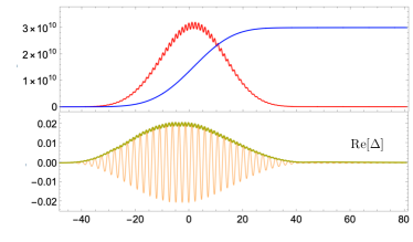
Figure 7: Temporal evolution of the excited density $n_{\mathrm{e}}(t)$ (red curve) and screening density $n_{\mathrm{pl}}(t)$ (blue curve) (panel a) and order parameter $\Delta(t)$ (panel b) in the TD-HSEX approximation.

The migration generates a plasma of free holes in the valence band and hence a nonvanishing $n_{\mathrm{pl}}$, see panel a (blue curve). In the early transient $t\lesssim-25$ fs the plasma density is very small and screening is negligible. According to the findings of the previous Section the system is in pure NEQ-EI state. As $n_{\mathrm{pl}}$ becomes sizable the electron-hole attraction is drastically reduced. The order parameter, see panel b, reaches a maximum value already at $t\approx-5$ fs, and then decays at a much faster rate than $1/2\tau_{\mathrm{K}}$ (the unscreened rate). To shed light on the physical scenario in this stage we calculate the transient spectral function.

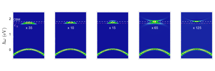
Figure 8: Transient spectral function $A_{{\mathbf{k}}}(\tau,\omega)$ evaluated with screening effects at different delays. The intensity from the conduction band is multiplied by the factor $M=S_{v}/S_{c}$ where $S_{\alpha}$ is the spectral weight of band $\alpha=v,c$ at ${\mathbf{k}}=0$. Energies are measured with respect to the the valence band maximum. Horizontal dashed lines at energies $\epsilon_{g}$ (white) and $\epsilon_{\mathrm{\rm x}}$ (red) are drawn to guide the eye.

In Fig. 8 we show $A_{{\mathbf{k}}}(\tau,\omega)$ for the same delays $\tau$ as in Fig. 5. For $\tau\lesssim 0$ the spectral function exhibits the typical feature of the NEQ-EI phase, with an excitonic replica of the valence band at energy $\epsilon_{\mathrm{\rm x}}<\epsilon_{g}$. For these delays the unscreened and screened spectral functions are almost identical. At delays $\tau\gtrsim 15$ fs a spectral structure right above the CBM develops. The appearance of this second structure in the spectral function points to a clear picture: excitons partially dissociate by breaking into e-h pairs at the K-point, with the free electrons occupying the empty levels around the CBM. Therefore excitons in the NEQ-EI phase and a plasma of free carriers coexist. As time increases the number of bound e-h pairs at the K-point becomes smaller and eventually the spectral weight is totally transferred to the conduction band. At delays $t\gtrsim 35$ fs only the conduction band is visible, implying that all carries are free. This incoherent regime lasts until the migration from K to $\Sigma$ is completed, i.e., until time $t\approx 40$ fs.

VII Conclusions and outlooks

We have studied the screened dynamics of the excitonic condensate forming in a bulk WSe₂ upon pumping in resonance with the lowest-energy exciton. Through the transient spectral function we have been able to observe the transition from an initial NEQ-EI phase of coherent excitons to a final phase of incoherent e-h pairs. This transition is not abrupt as the two phases coexist. The proposed theory relies on a general mechanism based on the interplay between intervalley scattering and plasma screening and the results agree with recent findings on the same system Puppin (2018). In fact, neglecting the renormalization of the effective e-h attraction the excitons at the K point would not break into e-h pairs at the same point and hence no signal from the conduction band would be detected at K. Furthermore, the maximum value of the density in the conduction band occurs at a delay $\tau$ which approaches zero with increasing the intensity of the pump pulse.

The screening due to quasi-free holes arising from the intervalley scattering is responsible for an ultrafast melting of the NEQ-EI phase. Although this mechanism has been highlighted in WSe₂ it is likely to occur in other indirect gap semiconductors as the only condition to meet is that electrons migrating from a local valley of the conduction band to the global CBM do not bounce back.

We have presented results based on a 2D two-band model. However the underlying theory can be implemented in available first-principles time-dependent codes Sangalli et al. (2019) to account explicitely for the spin-orbit interaction, the $\Sigma$ valley degrees of freedom as well as the phonon-induced intervalley scattering. The effective nonequilibrium e-h interaction is indeed screened adiabatically, hence retardation effects are discarded. In this work the interaction has been screened at the RPA level using the static 2D Lindhard function calculated at the density of the hole plasma – excitonic screening is negligible in the dilute limit Perfetto et al. (2020b). In first-principles implementations the nonequilibrium response function should instead be built taking into account the real band structure of the material.

Acknowledgements We acknowledge useful discussions with Andrea Marini and Davide Sangalli. We also acknowledge funding from MIUR PRIN Grant No. 20173B72NB and from INFN20-TIME2QUEST project. G.S. acknowledges Tor Vergata University for financial support through the Beyond Borders Project ULEXIEX.

Appendix A Self-consistent screening in the NEQ-EI superfluid

In the pure NEQ-EI state, i.e., the solution of the secular problem in Eq. (13), there is a finite density of conduction electrons $n_{\mathrm{e}}$ and valence holes $n_{\mathrm{h}}=n_{\mathrm{e}}$. It is therefore natural to ask whether in $\mathrm{WSe}_{2}$ bulk these excited carriers are capable to screen the e-h attraction such to disrupt the superfluid state and, eventually, to restore the normal phase. In a recent work Perfetto et al. (2020b) we have shown that the Coulomb repulsion $W^{\mathrm{ex}}$ screened by the excitonic condensate is given by

$$W^{\mathrm{ex}}_{{\mathbf{q}}}=\frac{U_{{\mathbf{q}}}}{1-U_{{\mathbf{q}}}(\chi^{{\mathbf{q}}}_{vv}+\chi^{{\mathbf{q}}}_{cc}+2\chi^{{\mathbf{q}}}_{vc})},$$ (26)

with the excitonic response function given by

$$\chi^{{\mathbf{q}}}_{\alpha\beta}=\frac{2}{\mbox{$\mathcal{N}$}}\sum_{{\mathbf{k}}}\left[\frac{\varphi^{+}_{\alpha{\mathbf{k}}+{\mathbf{q}}}\varphi^{+}_{\beta{\mathbf{k}}+{\mathbf{q}}}\varphi^{-}_{\alpha{\mathbf{k}}}\varphi^{-}_{\beta{\mathbf{k}}}}{-(e^{+}_{{\mathbf{k}}+{\mathbf{q}}}-e^{-}_{{\mathbf{k}}})+i\eta}\right.$$

$$-\left.\frac{\varphi^{-}_{\alpha{\mathbf{k}}+{\mathbf{q}}}\varphi^{-}_{\beta{\mathbf{k}}+{\mathbf{q}}}\varphi^{+}_{\alpha{\mathbf{k}}}\varphi^{+}_{\beta{\mathbf{k}}}}{-(e^{-}_{{\mathbf{k}}+{\mathbf{q}}}-e^{+}_{{\mathbf{k}}})+i\eta}\right].$$ (27)

Therefore the NEQ-EI state in the presence of the self-generated screening must be obtained by solving Eq. (13) by replacing $U_{{\mathbf{q}}}\to W^{\mathrm{ex}}_{{\mathbf{q}}}$. The resulting order parameter is displayed in Fig. 9. In order to highlight the impact of the excitonic screening we also show the points of Fig. 2 resulting from a self-consistent calculation with the bare interaction $U_{{\mathbf{q}}}$. We observe that for low densities $n_{\mathrm{e}}\lesssim\times 10^{11}\mathrm{cm}^{-2}$ screening effects are almost irrelevant. We recall that in the low-density regime all excited carriers participate to the creation of zero-momentum excitons, i.e. $N_{\mathrm{e}}=N_{\mathrm{ex}}$ (see Appendix B). The absence of free carriers and the fact that excitons are neutral bound states explain why in the dilute limit the screening efficiency is so scarce.

This result justifies the neglect of condensate screening in the numerical calculation of Figs. 3 and  7, where the maximum excited density is $n_{\rm e}\approx 6\times 10^{10}\mathrm{cm}^{-2}$ and $n_{\rm e}\approx 3\times 10^{10}\mathrm{cm}^{-2}$ respectively.

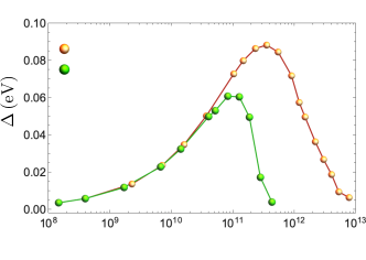
Figure 9: Order parameter with and without self-consistent excitonic screening versus electronic density $n_{\rm e}$.

Appendix B Proof of Eq. (21)

The NEQ-EI many-body state corresponding to the solution of the secular problem in Eq. (13) can be written as

$$|\Psi_{\mathrm{x}}\rangle=\prod_{{\mathbf{p}}\sigma}(\varphi^{-}_{v{\mathbf{p}}}\hat{f}^{{\dagger}}_{v{\mathbf{p}}\sigma}+\varphi^{-}_{c{\mathbf{p}}}\hat{f}^{{\dagger}}_{c{\mathbf{p}}\sigma})|0\rangle\,,$$ (28)

where $\hat{f}_{\mu{\mathbf{p}}\sigma}^{({\dagger})}$ annihilates (creates) an electron of momentum ${\mathbf{k}}$ with spin $\sigma$ in band $\mu=c,v$, and $|0\rangle$ is the electron vacuum. Let us consider the creation operator of an exciton with momentum ${\mathbf{q}}$

$$\hat{b}^{{\dagger}}_{{\mathbf{q}}}=\sum_{{\mathbf{k}}\sigma}Y^{{\mathbf{q}}}_{{\mathbf{k}}}\hat{f}^{{\dagger}}_{c{\mathbf{k}}\sigma}\hat{f}_{v{\mathbf{k}}\sigma},$$ (29)

where $Y^{{\mathbf{q}}}_{{\mathbf{k}}}$ is the excitonic wavefunction in momentum space, and define the total number of excitons with momentum ${\mathbf{q}}$ as

$$N_{\mathrm{ex},{\mathbf{q}}}\equiv\langle\Psi_{\mathrm{x}}|\hat{b}^{{\dagger}}_{{\mathbf{q}}}\hat{b}_{{\mathbf{q}}}|\Psi_{\mathrm{x}}\rangle.$$ (30)

It is matter of simple algebra to show that

$$N_{\mathrm{ex},{\mathbf{q}}} =2\delta_{{\mathbf{q}}\mathbf{0}}\left[\sum_{{\mathbf{k}}}(Y^{\mathbf{0}}_{{\mathbf{k}}}\rho^{cc}_{{\mathbf{k}}})^{2}+\sum_{{\mathbf{k}}\neq{\mathbf{k}}^{\prime}}Y^{\mathbf{0}}_{{\mathbf{k}}}Y^{\mathbf{0}}_{{\mathbf{k}}^{\prime}}\rho^{cv}_{{\mathbf{k}}}\rho^{vc}_{{\mathbf{k}}}\right]$$

$$+2(1-\delta_{{\mathbf{q}}\mathbf{0}})\sum_{{\mathbf{k}}}(Y^{{\mathbf{q}}}_{{\mathbf{k}}}\varphi^{-}_{c{\mathbf{k}}}\varphi^{-}_{c{\mathbf{k}}+{\mathbf{q}}})^{2}\,.$$ (31)

In the low-density limit the eigenvectors $\varphi^{-}_{\alpha{\mathbf{k}}}$ can be written in terms of the zero-momentum excitonic wavefunction $Y_{{\mathbf{q}}}\equiv Y^{\mathbf{0}}_{{\mathbf{k}}}$ using Eq. (19). Taking into account the normalization condition $\sum_{{\mathbf{k}}}|Y_{{\mathbf{k}}}|^{2}=1$ we find

$$N_{\mathrm{ex},{\mathbf{q}}}=\delta_{{\mathbf{q}}\mathbf{0}}N_{\mathrm{e}}+(1-\delta_{{\mathbf{q}}\mathbf{0}})N_{\mathrm{e}}^{2}\sum_{{\mathbf{k}}}(Y^{{\mathbf{q}}}_{{\mathbf{k}}}Y_{{\mathbf{k}}}Y_{{\mathbf{k}}+{\mathbf{q}}})^{2}\,.$$ (32)

It follows that $N_{\mathrm{ex},\mathbf{0}}\equiv N_{\mathrm{ex}}=N_{\mathrm{e}}$ diverges in the thermodynamic limit for any finite electron density $n_{\rm e}$. The number of nonvanishing momentum excitons $N_{\mathrm{ex}{\mathbf{q}}\neq\mathbf{0}}$ is instead of order $\mbox{$\mathcal{O}$}(\mbox{$\mathcal{N}$}^{0})$.

Appendix C Evaluation of the transient spectral function

The tr-ARPES signal is proportional to the number of electrons $N_{{\mathbf{k}}}(\omega)$ with energy $\omega$ and parallel momentum ${\mathbf{k}}$ ejected by a probe pulse. For an arbitrary probe pulse of temporal profile $e(t)$ we have Perfetto et al. (2016); Freericks et al. (2009)

$$N_{{\mathbf{k}}}(\omega)=2\sum_{\mu\nu}\int dt_{1}dt_{2}\;{\rm Re}\left[\Sigma^{\mu\nu,\rm R}_{{\mathbf{k}},\omega}(t_{1},t_{2})G^{\nu\mu,<}_{{\mathbf{k}}}(t_{2},t_{1})\right].$$ (33)

Here $G^{\nu\mu,<}_{{\mathbf{k}}}(t_{2},t_{1})$ is the (spin-independent) lesser Green’s function defined as Stefanucci and van Leeuwen (2013)

$$G^{\nu\mu,<}_{{\mathbf{k}}}(t_{2},t_{1})=\langle\hat{f}^{{\dagger}}_{\mu{\mathbf{k}}\sigma}(t_{1})\hat{f}_{\nu{\mathbf{k}}\sigma}(t_{2})\rangle\,,$$ (34)

with time dependent operators $\hat{f}^{({\dagger})}_{\mu{\mathbf{k}}\sigma}(t)$ in the Heisenberg picture. The ionization self-energy reads Perfetto et al. (2015)

$$\Sigma^{\mu\nu,\rm R}_{{\mathbf{k}},\omega}(t_{1},t_{2})=-i\theta(t_{1}-t_{2})d_{{\mathbf{k}},\omega}^{\mu}e(t_{1})e^{-i\omega(t_{1}-t_{2})}d_{{\mathbf{k}},\omega}^{\nu}e(t_{2})$$ (35)

where $d_{{\mathbf{k}},\omega}^{\mu}$ is the dipole matrix element between a state in band $\mu$ and momentum ${\mathbf{k}}$ and a continuum time-reversed LEED state of energy $\omega$ and parallel momentum ${\mathbf{k}}$.

From Eq. (33) we see that $N_{{\mathbf{k}}}(\omega)$ is a complicated two-times convolution of $G^{<}$. However a simpler and more transparent expression can be obtained if the probe pulse has a duration $t_{p}$ much longer than the typical electronic timescale and a frequency $\omega_{p}$ large enough to resolve the desired removal energies. In this case one can shown that Eq. (33) reduces to Perfetto et al. (2020a)

$$N_{{\mathbf{k}}}(\omega)\propto A_{{\mathbf{k}}}(\tau,\omega-\omega_{p})$$ (36)

where $\tau$ is the time at which the probe impinges the system and transient spectral function

$$A_{{\mathbf{k}}}(\tau,\omega)=-i\int_{\tau-t_{p}/2}^{\tau+t_{p}/2}d\bar{t}\,e^{i\omega\bar{t}}\,\mathrm{Tr}[G^{<}_{{\mathbf{k}}}(\tau-\bar{t},\tau+\bar{t})].$$ (37)

In bulk $\mathrm{WSe}_{2}$ excited by a VIS pump the density matrix varies in time no slower than a timescale of $\sim 2$ fs, given by the inverse of the lowest exciton energy $\epsilon_{\mathrm{x}}$. The approximated expression in Eq. (37) can be safely used if the XUV probe has central frequency $\omega_{p}\approx 20$ eV and total duration $t_{p}\approx 70$ fs (FWHM = 35 fs) .

To obtain the lesser Green’s function $G^{<}$ from the numerical solution of Eq. (8) we use the relation Lipavský et al. (1986)

$$G_{{\mathbf{k}}}^{<}(t,t^{\prime})=-G_{{\mathbf{k}}}^{R}(t^{\prime},t^{\prime})\rho_{{\mathbf{k}}}(t)+\rho_{{\mathbf{k}}}(t)G_{{\mathbf{k}}}^{\rm A}(t,t^{\prime})\,.$$ (38)

Here the retarded Green’s function reads Latini et al. (2014)

$$G^{\rm R}_{{\mathbf{k}}}(t,t^{\prime})=-i\theta(t,t^{\prime})\mbox{$\mathcal{T}$}\left\{e^{-i\int_{t^{\prime}}^{t}d\bar{t}[h_{\mathrm{HSEX},{\mathbf{k}}}(t)-i\Gamma/2]}\right\}\,,$$ (39)

where $\mathcal{T}$ is the time-ordering operator and $G^{\rm R}_{{\mathbf{k}}}(t,t^{\prime})=[G^{\rm A}_{{\mathbf{k}}}(t^{\prime},t)]^{\ast}$.

References

- Keldysh (1972) L. Keldysh, Problems of theoretical physics (1972).
- Keldysh and Kozlov (1968) L. V. Keldysh and A. N. Kozlov, JETP 27, 521 (1968).
- Moskalenko and Snoke (2000) S. A. Moskalenko and D. W. Snoke, Bose-Einstein Condensation of Excitons and Biexcitons (2000).
- Combescot and Shiau (2016) M. Combescot and S. Shiau, Excitons and Cooper Pairs: Two Composite Bosons in Many-body Physics, Oxford graduate texts (Oxford University Press, 2016), ISBN 9780198753735, URL https://books.google.it/books?id=YzAiCwAAQBAJ.
- Schmitt-Rink et al. (1988) S. Schmitt-Rink, D. S. Chemla, and H. Haug, Phys. Rev. B 37, 941 (1988), URL https://link.aps.org/doi/10.1103/PhysRevB.37.941.
- Kuklinski and Mukamel (1990) J. R. Kuklinski and S. Mukamel, Physical Review B 42, 2959 (1990).
- Glutsch and Zimmermann (1992) S. Glutsch and R. Zimmermann, Phys. Rev. B 45, 5857 (1992), URL https://link.aps.org/doi/10.1103/PhysRevB.45.5857.
- Littlewood and Zhu (1996) P. Littlewood and X. Zhu, Physica Scripta 1996, 56 (1996).
- Östreich and Schönhammer (1993) T. Östreich and K. Schönhammer, Zeitschrift für Physik B Condensed Matter 91, 189 (1993), URL https://doi.org/10.1007/BF01315235.
- Hannewald et al. (2000) K. Hannewald, S. Glutsch, and F. Bechstedt, Journal of Physics: Condensed Matter 13, 275 (2000), URL https://doi.org/10.1088%2F0953-8984%2F13%2F2%2F305.
- Glutsch et al. (1992) S. Glutsch, F. Bechstedt, and R. Zimmermann, physica status solidi (b) 172, 357 (1992), eprint https://onlinelibrary.wiley.com/doi/pdf/10.1002/pssb.2221720131, URL https://onlinelibrary.wiley.com/doi/abs/10.1002/pssb.2221720131.
- Perfetto et al. (2019) E. Perfetto, D. Sangalli, A. Marini, and G. Stefanucci, Phys. Rev. Materials 3, 124601 (2019), URL https://link.aps.org/doi/10.1103/PhysRevMaterials.3.124601.
- Szymańska et al. (2006) M. H. Szymańska, J. Keeling, and P. B. Littlewood, Phys. Rev. Lett. 96, 230602 (2006), URL https://link.aps.org/doi/10.1103/PhysRevLett.96.230602.
- Hanai et al. (2016) R. Hanai, P. B. Littlewood, and Y. Ohashi, Journal of Low Temperature Physics 183, 127 (2016), URL https://doi.org/10.1007/s10909-016-1552-6.
- Hanai et al. (2017) R. Hanai, P. B. Littlewood, and Y. Ohashi, Phys. Rev. B 96, 125206 (2017), URL https://link.aps.org/doi/10.1103/PhysRevB.96.125206.
- Triola et al. (2017) C. Triola, A. Pertsova, R. S. Markiewicz, and A. V. Balatsky, Phys. Rev. B 95, 205410 (2017), URL https://link.aps.org/doi/10.1103/PhysRevB.95.205410.
- Hanai et al. (2018) R. Hanai, P. B. Littlewood, and Y. Ohashi, Phys. Rev. B 97, 245302 (2018), URL https://link.aps.org/doi/10.1103/PhysRevB.97.245302.
- Pertsova and Balatsky (2018) A. Pertsova and A. V. Balatsky, Phys. Rev. B 97, 075109 (2018), URL https://link.aps.org/doi/10.1103/PhysRevB.97.075109.
- Becker et al. (2019) K. W. Becker, H. Fehske, and V.-N. Phan, Phys. Rev. B 99, 035304 (2019), URL https://link.aps.org/doi/10.1103/PhysRevB.99.035304.
- Yamaguchi et al. (2013) M. Yamaguchi, K. Kamide, R. Nii, T. Ogawa, and Y. Yamamoto, Phys. Rev. Lett. 111, 026404 (2013), URL https://link.aps.org/doi/10.1103/PhysRevLett.111.026404.
- Pertsova and Balatsky (2020) A. Pertsova and A. V. Balatsky, Annalen der Physik 532, 1900549 (2020).
- Christiansen et al. (2019) D. Christiansen, M. Selig, E. Malic, R. Ernstorfer, and A. Knorr, Phys. Rev. B 100, 205401 (2019), URL https://link.aps.org/doi/10.1103/PhysRevB.100.205401.
- Perfetto et al. (2020a) E. Perfetto, S. Bianchi, and G. Stefanucci, Phys. Rev. B 101, 041201 (2020a), URL https://link.aps.org/doi/10.1103/PhysRevB.101.041201.
- Madéo et al. (2020) J. Madéo, M. K. Man, C. Sahoo, M. Campbell, V. Pareek, E. L. Wong, A. A. Mahboob, N. S. Chan, A. Karmakar, B. M. K. Mariserla, et al., arXiv preprint arXiv:2005.00241 (2020).
- Lee et al. (2020) W. Lee, Y. Lin, L.-S. Lu, W.-C. Chueh, M. Liu, X. Li, W.-H. Chang, R. A. Kaindl, and C.-K. Shih, arXiv preprint arXiv:2008.06103 (2020).
- Koch et al. (2006) S. W. Koch, M. Kira, G. Khitrova, and H. M. Gibbs, Nature Materials 5, 523 (2006), URL https://doi.org/10.1038/nmat1658.
- Madrid et al. (2009) A. B. Madrid, K. Hyeon-Deuk, B. F. Habenicht, and O. V. Prezhdo, ACS nano 3, 2487 (2009).
- Nie et al. (2014) Z. Nie, R. Long, L. Sun, C.-C. Huang, J. Zhang, Q. Xiong, D. W. Hewak, Z. Shen, O. V. Prezhdo, and Z.-H. Loh, ACS nano 8, 10931 (2014).
- Selig et al. (2016) M. Selig, G. Berghäuser, A. Raja, P. Nagler, C. Schüller, T. F. Heinz, T. Korn, A. Chernikov, E. Malic, and A. Knorr, Nature Communications 7, 13279 (2016), URL https://doi.org/10.1038/ncomms13279.
- Sangalli et al. (2018) D. Sangalli, E. Perfetto, G. Stefanucci, and A. Marini, The European Physical Journal B 91, 171 (2018).
- Chernikov et al. (2015a) A. Chernikov, A. M. van der Zande, H. M. Hill, A. F. Rigosi, A. Velauthapillai, J. Hone, and T. F. Heinz, Phys. Rev. Lett. 115, 126802 (2015a), URL https://link.aps.org/doi/10.1103/PhysRevLett.115.126802.
- Chernikov et al. (2015b) A. Chernikov, C. Ruppert, H. M. Hill, A. F. Rigosi, and T. F. Heinz, Nature Photonics 9, 466 (2015b), URL https://doi.org/10.1038/nphoton.2015.104.
- Cunningham et al. (2017) P. D. Cunningham, A. T. Hanbicki, K. M. McCreary, and B. T. Jonker, ACS Nano 11, 12601 (2017), URL https://doi.org/10.1021/acsnano.7b06885.
- Yao et al. (2017) K. Yao, A. Yan, S. Kahn, A. Suslu, Y. Liang, E. S. Barnard, S. Tongay, A. Zettl, N. J. Borys, and P. J. Schuck, Phys. Rev. Lett. 119, 087401 (2017), URL https://link.aps.org/doi/10.1103/PhysRevLett.119.087401.
- Wang et al. (2019) J. Wang, J. Ardelean, Y. Bai, A. Steinhoff, M. Florian, F. Jahnke, X. Xu, M. Kira, J. Hone, and X.-Y. Zhu, Science Advances 5 (2019), URL https://advances.sciencemag.org/content/5/9/eaax0145.
- Dendzik et al. (2020) M. Dendzik, R. P. Xian, E. Perfetto, D. Sangalli, D. Kutnyakhov, S. Dong, S. Beaulieu, T. Pincelli, F. Pressacco, D. Curcio, et al., Phys. Rev. Lett. 125, 096401 (2020), URL https://link.aps.org/doi/10.1103/PhysRevLett.125.096401.
- Perfetto et al. (2016) E. Perfetto, D. Sangalli, A. Marini, and G. Stefanucci, Phys. Rev. B 94, 245303 (2016), URL https://link.aps.org/doi/10.1103/PhysRevB.94.245303.
- Steinhoff et al. (2017) A. Steinhoff, M. Florian, M. Rösner, G. Schönhoff, T. O. Wehling, and F. Jahnke, Nature Communications 8, 1166 (2017), URL https://doi.org/10.1038/s41467-017-01298-6.
- Rustagi and Kemper (2018) A. Rustagi and A. F. Kemper, Phys. Rev. B 97, 235310 (2018), URL https://link.aps.org/doi/10.1103/PhysRevB.97.235310.
- Jiang (2012) H. Jiang, The Journal of Physical Chemistry C 116, 7664 (2012), eprint https://doi.org/10.1021/jp300079d, URL https://doi.org/10.1021/jp300079d.
- Beal and Liang (1976) A. Beal and W. Liang, Journal of Physics C: Solid State Physics 9, 2459 (1976).
- Finteis et al. (1997) T. Finteis, M. Hengsberger, T. Straub, K. Fauth, R. Claessen, P. Auer, P. Steiner, S. Hüfner, P. Blaha, M. Vögt, et al., Phys. Rev. B 55, 10400 (1997), URL https://link.aps.org/doi/10.1103/PhysRevB.55.10400.
- Arora et al. (2015) A. Arora, M. Koperski, K. Nogajewski, J. Marcus, C. Faugeras, and M. Potemski, Nanoscale 7, 10421 (2015).
- Riley et al. (2015) J. M. Riley, W. Meevasana, L. Bawden, M. Asakawa, T. Takayama, T. Eknapakul, T. Kim, M. Hoesch, S.-K. Mo, H. Takagi, et al., Nature nanotechnology 10, 1043 (2015).
- Kim et al. (2016) B. S. Kim, J.-W. Rhim, B. Kim, C. Kim, and S. R. Park, Scientific reports 6, 36389 (2016).
- Frindt (1963) R. Frindt, Journal of Physics and Chemistry of Solids 24, 1107 (1963).
- Wang et al. (2018) G. Wang, A. Chernikov, M. M. Glazov, T. F. Heinz, X. Marie, T. Amand, and B. Urbaszek, Rev. Mod. Phys. 90, 021001 (2018), URL https://link.aps.org/doi/10.1103/RevModPhys.90.021001.
- Bertoni et al. (2016) R. Bertoni, C. W. Nicholson, L. Waldecker, H. Hübener, C. Monney, U. De Giovannini, M. Puppin, M. Hoesch, E. Springate, R. T. Chapman, et al., Phys. Rev. Lett. 117, 277201 (2016), URL https://link.aps.org/doi/10.1103/PhysRevLett.117.277201.
- Steinhoff et al. (2014) A. Steinhoff, M. Rösner, F. Jahnke, T. O. Wehling, and C. Gies, Nano Letters 14, 3743 (2014), URL https://doi.org/10.1021/nl500595u.
- Liang and Yang (2015) Y. Liang and L. Yang, Phys. Rev. Lett. 114, 063001 (2015), URL https://link.aps.org/doi/10.1103/PhysRevLett.114.063001.
- Meckbach et al. (2018) L. Meckbach, T. Stroucken, and S. W. Koch, Applied Physics Letters 112, 061104 (2018), URL https://doi.org/10.1063/1.5017069.
- Puppin (2018) M. Puppin, Phd thesis (2018), URL http://dx.doi.org/10.17169/refubium-804.
- Latini et al. (2015) S. Latini, T. Olsen, and K. S. Thygesen, Phys. Rev. B 92, 245123 (2015), URL https://link.aps.org/doi/10.1103/PhysRevB.92.245123.
- Wallauer et al. (2016) R. Wallauer, J. Reimann, N. Armbrust, J. Güdde, and U. Höfer, Applied Physics Letters 109, 162102 (2016).
- Waldecker et al. (2017) L. Waldecker, R. Bertoni, H. Hübener, T. Brumme, T. Vasileiadis, D. Zahn, A. Rubio, and R. Ernstorfer, Physical Review Letters 119, 036803 (2017).
- Haug et al. (1994) H. Haug, , and S. W. Koch, Quantum Theory of the Optical and Electronic Properties of Semiconductors (World Scientific, Singapore, 1994).
- Steinhoff et al. (2016) A. Steinhoff, M. Florian, M. Rösner, M. Lorke, T. O. Wehling, C. Gies, and F. Jahnke, 2D Materials 3, 031006 (2016), URL https://doi.org/10.1088%2F2053-1583%2F3%2F3%2F031006.
- Schmidt et al. (2016) R. Schmidt, G. Berghauser, R. Schneider, M. Selig, P. Tonndorf, E. Malic, A. Knorr, S. Michaelis de Vasconcellos, and R. Bratschitsch, Nano letters 16, 2945 (2016).
- Molina-Sánchez et al. (2017) A. Molina-Sánchez, D. Sangalli, L. Wirtz, and A. Marini, Nano Letters 17, 4549 (2017), URL https://doi.org/10.1021/acs.nanolett.7b00175.
- Perfetto et al. (2020b) E. Perfetto, A. Marini, and G. Stefanucci, Phys. Rev. B 102, 085203 (2020b), URL https://link.aps.org/doi/10.1103/PhysRevB.102.085203.
- Giuliani and Vignale (2005) G. Giuliani and G. Vignale, Quantum Theory of the Electron Liquid (Cambridge University Press, Cambridge, 2005).
- Halperin and Rice (1968) B. Halperin and T. Rice, Solid State Physics 21, 115 (1968), URL http://www.sciencedirect.com/science/article/pii/S0081194708607407.
- Blatt et al. (1962) J. M. Blatt, K. W. Böer, and W. Brandt, Phys. Rev. 126, 1691 (1962), URL https://link.aps.org/doi/10.1103/PhysRev.126.1691.
- Keldysh and Kopaev (1965) L. V. Keldysh and Y. U. Kopaev, Sov. Phys. Solid State 6, 2219 (1965).
- Kozlov and Maksimov (1965) A. N. Kozlov and L. A. Maksimov, JETP 21, 790 (1965).
- Jérome et al. (1967) D. Jérome, T. M. Rice, and W. Kohn, Phys. Rev. 158, 462 (1967), URL https://link.aps.org/doi/10.1103/PhysRev.158.462.
- Comte, C. and Nozières, P. (1982) Comte, C. and Nozières, P., J. Phys. France 43, 1069 (1982), URL https://doi.org/10.1051/jphys:019820043070106900.
- Perfetto and Stefanucci (2020) E. Perfetto and G. Stefanucci, Phys. Rev. Lett. 125, 106401 (2020), URL https://link.aps.org/doi/10.1103/PhysRevLett.125.106401.
- Perfetto and Stefanucci (2018) E. Perfetto and G. Stefanucci, Journal of Physics: Condensed Matter 30, 465901 (2018), URL http://stacks.iop.org/0953-8984/30/i=46/a=465901.
- Sangalli et al. (2019) D. Sangalli, A. Ferretti, H. Miranda, C. Attaccalite, I. Marri, E. Cannuccia, P. Melo, M. Marsili, F. Paleari, A. Marrazzo, et al., Journal of Physics: Condensed Matter 31, 325902 (2019), URL https://doi.org/10.1088%2F1361-648x%2Fab15d0.
- Freericks et al. (2009) J. K. Freericks, H. R. Krishnamurthy, and T. Pruschke, Phys. Rev. Lett. 102, 136401 (2009), URL https://link.aps.org/doi/10.1103/PhysRevLett.102.136401.
- Stefanucci and van Leeuwen (2013) G. Stefanucci and R. van Leeuwen, Nonequilibrium Many-Body Theory of Quantum Systems: A Modern Introduction (Cambridge University Press, Cambridge, 2013).
- Perfetto et al. (2015) E. Perfetto, A.-M. Uimonen, R. van Leeuwen, and G. Stefanucci, Phys. Rev. A 92, 033419 (2015), URL https://link.aps.org/doi/10.1103/PhysRevA.92.033419.
- Lipavský et al. (1986) P. Lipavský, V. Špička, and B. Velický, Phys. Rev. B 34, 6933 (1986), URL https://link.aps.org/doi/10.1103/PhysRevB.34.6933.
- Latini et al. (2014) S. Latini, E. Perfetto, A.-M. Uimonen, R. van Leeuwen, and G. Stefanucci, Phys. Rev. B 89, 075306 (2014), URL https://link.aps.org/doi/10.1103/PhysRevB.89.075306.