Provably robust blind source separation of
linear-quadratic near-separable mixtures

Abstract

In this work, we consider the problem of blind source separation (BSS) by departing from the usual linear model and focusing on the linear-quadratic (LQ) model. We propose two provably robust and computationally tractable algorithms to tackle this problem under separability assumptions which require the sources to appear as samples in the data set. The first algorithm generalizes the successive nonnegative projection algorithm (SNPA), designed for linear BSS, and is referred to as SNPALQ. By explicitly modeling the product terms inherent to the LQ model along the iterations of the SNPA scheme, the nonlinear contributions of the mixing are mitigated, thus improving the separation quality. SNPALQ is shown to be able to recover the ground truth factors that generated the data, even in the presence of noise. The second algorithm is a brute-force (BF) algorithm, which is used as a post-processing step for SNPALQ. It enables to discard the spurious (mixed) samples extracted by SNPALQ, thus broadening its applicability. The BF is in turn shown to be robust to noise under easier-to-check and milder conditions than SNPALQ. We show that SNPALQ with and without the BF postprocessing is relevant in realistic numerical experiments.

15A23, 65F55, 68Q25, 65D18

1 Introduction

Blind source separation (BSS) [comon2010handbook, bobin2015sparsity, kervazo2018PALM] is a powerful paradigm with a wide range of applications such as remote sensing [Schaepman2009], biomedical and pharmaceutical imaging [Akbari2011, Rodionova2005], and astronomy [Themelis2012]. BSS aims at decomposing a given data set into a set of unknown elementary signals to be recovered, generally referred to as the sources. Because it is simple and easily interpretable, many works [comon2010handbook] have focused on the linear mixing model (LMM) which assumes that the $i$th data set sample $\bar{\mathbf{x}}_{i}\in\mathbb{R}^{m}$ for $i\in[\![n]\!]$ can be written as

$$\bar{\mathbf{x}}_{i}=\sum_{k=1}^{r}h_{ki}\mathbf{w}_{k}+\mathbf{n}_{i},$$

where $\mathbf{w}_{k}$ is the $k$th source for $k\in[\![r]\!]=\{1,2,\dots,r\}$, and $h_{ki}$ its the associated mixing coefficient in the $i$th (mixed) observation. The vector $\mathbf{n}_{i}$ accounts for any additive noise and/or slight mismodelings in the $i$th pixel. Using a standard matrix formulation, the LMM can thus be rewritten as

$$\bar{\mathbf{X}}=\mathbf{W}\mathbf{H}+\mathbf{N},$$

where $\bar{\mathbf{X}}=[\bar{\mathbf{x}}_{1},\bar{\mathbf{x}}_{2},...,\bar{\mathbf{x}}_{m}]\in\mathbb{R}^{m\times n}$ is the data set, $\mathbf{W}=[\mathbf{w}_{1},\mathbf{w}_{2},...,\mathbf{w}_{r}]\in\mathbb{R}^{m\times r}$ are the sources, $\mathbf{H}\in\mathbb{R}^{r\times n}$ is the mixing matrix containing the coefficients $h_{ki}$’s, and $\mathbf{N}=[\mathbf{n}_{1},\mathbf{n}_{2},...,\mathbf{n}_{m}]\in\mathbb{R}^{m\times n}$ is the noise. We denote by $\mathbf{X=WH}$ the noiseless version of $\bar{\mathbf{X}}$.

The goal of BSS is to recover $\mathbf{W}$ and $\mathbf{H}$ from the sole knowledge of $\bar{\mathbf{X}}$. This is in general an ill-posed problem [comon2010handbook]. Hence, in most works, additional constraints are imposed on the unknown matrices $\mathbf{W}$ and $\mathbf{H}$ to make the problem better posed: for instance, orthogonality in principal component analysis (PCA – [jolliffe1986principal]), independence in independent component analysis (ICA – [comon2010handbook]), and sparsity in sparse component analysis (SCA – [zibulevsky2001blind, bobin2015sparsity, kervazo2018PALM]). We will here focus on nonnegativity constraints, akin to nonnegative matrix factorization (NMF) [lee1999learning]. Although NMF is NP-hard in general [vavasis2010complexity], and its solution non-unique [xiao2019uniq], Arora et al. [AGKM11, Arora2016] have introduced the subclass of near-separable non-negative matrices for which NMF can be solved in a polynomial time with weak indeterminacies. This subclass corresponds to data sets in which each source appears purely in at least one data sample. Building on near-separable NMF, several provably robust algorithms have been proposed [AGKM11, Esser2012convex, Recht2012, gillis2014robust]. Among them, one can cite the successive projection algorithm (SPA) [Araujo01], which is a fast greedy algorithm provably robust to noise [Gillis_12_FastandRobust], or an enhanced version, the successive nonnegative projection algorithm (SNPA) [Gillis2014], which is more efficient when $\mathbf{W}$ is ill-conditioned and is applicable when $\mathbf{W}$ is rank-deficient.

1.1 LQ mixing model

In various applications, the LMM may however suffer from some limitations and can only be considered as a first-order approximation of non-linear mixing models [Bioucas-Dias2012, dobigeon2014nonlinear, Dobigeon2016]. In such situations, linear-quadratic (LQ) [Deville2019] models can for instance better account for the physical mixing processes by including termwise products of the sources [Dobigeon2014, Heylen2014]. This model can be written as

(1) $$\bar{\mathbf{x}}_{i}=\sum_{k=1}^{r}h_{ki}\mathbf{w}_{k}+\sum_{p=1}^{r}\sum_{l=p}^{r}\beta_{ipl}(\mathbf{w}_{p}\odot\mathbf{w}_{l})+\mathbf{n}_{i}.$$

In (1), the linear contribution associated to LMM is complemented by a set of second-order interactions $\mathbf{w}_{p}\odot\mathbf{w}_{l}$ between the sources, where $\odot$ denotes the Hadamard product and $\beta_{ipl}$ is the amount of the interaction $\mathbf{w}_{p}\odot\mathbf{w}_{l}$ within the $i$th observation. It is worth mentioning the closely-related so-called bilinear mixing model [dobigeon2014nonlinear, Deville2019], which is a particular instance of the LQ mixing model, from which the squared terms $\mathbf{w}_{p}\odot\mathbf{w}_{p}$ for $p\in[\![r]\!]$ in (1) are removed; see Application 1.1 below for a discussion in the context of blind hyperspectral unmixing where the LQ and bilinear models are widely used.

The LQ mixing model (1) can also be rewritten in a matrix form

(2) $$\bar{\mathbf{X}}=\Pi_{2}(\mathbf{W}){\mathbf{H}}+\mathbf{N}$$

where $\Pi_{2}(\mathbf{W})\in\mathbb{R}^{m\times\tilde{r}}$ is the extended source matrix containing the sources and their second-order products as its columns, with $\tilde{r}={r(r+3)}/{2}$, and ${\mathbf{H}}\in\mathbb{R}^{\tilde{r}\times n}$ is the matrix gathering all the mixing coefficients associated with the linear ($h_{ki}$’s) and nonlinear ($\beta_{ipl}$’s) contributions. Written in such a matrix form, the similarity between the LQ and linear models is easily visible: the LQ mixings can be written in a linear form by considering the quadratic terms $\mathbf{w}_{p}\odot\mathbf{w}_{l}$ as new sources, additional to the usual ones $\mathbf{w}_{k}$. Following this line of thought, the $\mathbf{w}_{p}\odot\mathbf{w}_{l}$ terms are often called virtual sources. In the sequel of this paper, this terminology will be adopted and the non-virtual sources $\mathbf{w}_{i}$ will be referred to as primary.

[Hyperspectral imaging] To illustrate the BSS of LQ-mixtures (LQ-BSS), we consider throughout this paper the example of hyperspectral (HS) imaging. Despite having a finer spectral resolution than conventional natural images, HS images generally suffer from a limited spatial resolution. Therefore, several materials are generally present in each pixel, and thus the acquired spectra correspond to mixtures of the different pure material spectra, called endmembers. This mandates the use of BSS methods – more specifically of NMF – to perform spectral unmixing. To be more precise, using the terminology of HS unmixing [dobigeon2014nonlinear], $\mathbf{w}_{k}$ in (1) corresponds to the spectral signature of the $k$th endmember and $h_{ki}$ to the abundance of the $k$th endmember in the $i$th pixel. The spectral signature of a source is the fraction of light reflected by that source depending on the wavelength, and hence $0\leq\mathbf{w}_{k}\leq 1$ for $k\in[\![r]\!]$. Concerning the model choice, the linear BSS model is often a too rough approximation in HS: in particular, when the light arriving on the sensor interacts with several materials, nonlinear mixing effects may occur [Bioucas-Dias2012, dobigeon2014nonlinear, Dobigeon2016]. Specifically, this is often the case when the scene is not flat, for instance in the presence of large geometric structures, such as in urban [meganem2014linear] or forest [Dobigeon2014] scenes. In such a context, it has been shown [Dobigeon2014, Heylen2014] that LQ models enable to better account for multiple scatterings. While it is further possible to include higher-order terms, most of the works neglect the interactions of order larger than two since they are expected to be of significantly lower magnitudes [Altmann2012, Meganem2013] as $0\leq\mathbf{W}\leq 1$.

1.2 Identifiability issue in LQ-BSS

Despite source identifiability issues in the general context of non-linear BSS problems [comon2010handbook, deville2015overview, kervazo2019nonlin], it was recently showed [Deville2019] that the non-linearity inherent to bilinear mixtures leads to an essentially unique solution in the noiseless case. More precisely, it was shown that for a data matrix $\mathbf{X}$ following the bilinear model in the absence of noise (and under some appropriate assumptions, see below), any $\hat{\mathbf{W}}$ and $\hat{\mathbf{H}}$ such that $\mathbf{X}=\Pi_{2}(\hat{\mathbf{W}})\hat{\mathbf{H}}$ satisfy $\hat{\mathbf{W}}=\mathbf{W}$ and $\hat{\mathbf{H}}=\mathbf{H}$ up to a scaling and permutation of the columns of $\hat{\mathbf{W}}$ and the rows of $\hat{\mathbf{H}}$. However, this identifiability result suffers from some limitations:

• It relies on two strong assumptions:

  1. $\operatorname*{rowrank}(\mathbf{X})=\frac{r(r+1)}{2}$, requiring that $\hat{\mathbf{H}}$ has full row rank and hence that every extended source is present in the data set. In other words, all possible interactions of two primary sources must be present in some observation. This is unlikely to happen in practice.

  2. the products of the sources up to order four must be linearly independent. It requires the family

     (3) $$\small\left(\mathbf{W},(\mathbf{w}_{i}\odot\mathbf{w}_{j})_{\begin{subarray}{c}i,j\in[\![r]\!]\\ j<i\end{subarray}},(\mathbf{w}_{i}\odot\mathbf{w}_{j}\odot\mathbf{w}_{k})_{\begin{subarray}{c}i,j,k\in[\![r]\!]\\ k<j<i\end{subarray}},(\mathbf{w}_{i}\odot\mathbf{w}_{j}\odot\mathbf{w}_{k}\odot\mathbf{w}_{l})_{\begin{subarray}{c}i,j,k,l\in[\![r]\!]\\ l<k<j<i\end{subarray}}\right),$$

     to be linearly independent. As its size is $\frac{r(r+1)}{24}\big{(}(r-1)(r-2)+12\big{)}$, such a linear independence assumption might not be satisfied in real-world scenarios, since the number of observations $m$ must be of order $\Theta(r^{4})$.

• It does not apply to mixings with squared terms [Deville2019, section 7], that is, LQ mixings instead of bilinear ones.

• No guarantee is given in the presence of noise. Moreover, finding an exact factorization $\Pi_{2}(\hat{\mathbf{W}})\hat{\mathbf{H}}$ of $\mathbf{X}$ is a difficult problem. The algorithm used in [Deville2019] is a heuristic and does not find an exact solution (see [Deville2019, Fig. 4]), leading to errors on the recovered sources.

[Hyperspectral imaging (cont’d)] In HS imaging, the assumption that $\mathbf{H}$ has full row rank is unlikely to be satisfied as many endmembers do not interact, because they are located far apart in the image.

For the second assumption, even with $r=10$ endmembers, which is a relatively small number, at least $m\geq 385$ spectral bands would be required to ensure the linear independence of the family (3). This is not satisfied for typical HS sensors dedicated to Earth observation. As an example, the Airborne Visible / Infrared Imaging Spectrometer (AVIRIS) operated by the Jet Propulsion Laboratory (JPL, NASA), acquires HS images composed of $m=224$ spectral bands, among them several dozens are inexploitable due to low signal-to-noise ratios.

1.3 Near-separable LQ mixings

To overcome the above identifiability issues, we propose in this work to tackle BSS problems of the form (1) under a near-separable NMF-like paradigm. In particular, the rationale is to convert the linear independence condition on the family (3) into a non-negative independence condition, which is significantly less restrictive. Consider for instance the family of points located on a circle within the unit simplex in three dimensions, that is, distinct points within the set $\{\mathbf{x}\in\mathbb{R}^{3}_{+}\ |\ \|\mathbf{x}\|_{1}=1,\|\mathbf{x}\|_{2}=q\}$ for some $q<1$. Although the rank of this family is 3, no point is within the convex cone of other points, and hence this family is non-negatively independent.

More specifically, denoting $\Delta=\{\mathbf{x}\in\mathbb{R}^{\tilde{r}}|x\geq 0,\sum_{i=1}^{\tilde{r}}x_{i}\leq 1\}$ and $\Pi_{2}(\mathbf{W})_{\setminus\{j\}}$ the submatrix of $\Pi_{2}(\mathbf{W})$ excluding $\mathbf{w}_{j}$, we assume the following constraints:

$$h_{ki}\geq 0\text{ for all }i\in[\![n]\!]\text{ and }k\in[\![\tilde{r}]\!]\text{ (nonnegativity condition)},$$

(4) $$\sum_{k=1}^{\tilde{r}}h_{ki}\leq 1\text{ for all }i\in[\![n]\!]\text{ (sum to at most one condition)},$$

$$\alpha_{2}(\mathbf{W})=\min_{j\in[\![r]\!]}\min_{\mathbf{x}\in\Delta}\left\|{\mathbf{w}_{j}-\Pi_{2}(\mathbf{W})_{\setminus\{j\}}\mathbf{x}}\right\|_{2}>0\text{ (order-2 }\alpha\text{-robust simplicial}).$$

The two first constraints ensure the mixing coefficients for each pixel to be nonnegative and to sum to at most one, and can be equivalently written as $\mathbf{h}_{i}\in\Delta$ for all $i\in[\![\tilde{r}]\!]$. The last one ensures that no source lies within the convex hull formed by the other ones, their second order product and the origin. It is thus an extension of the $\alpha$-robust simplicial definition of [Arora2016] which requires that $\alpha_{1}(\mathbf{W})=\min_{j\in[\![r]\!]}\min_{\mathbf{x}\in\Delta}\left\|{\mathbf{w}_{j}-\mathbf{W}_{\setminus\{j\}}\mathbf{x}}\right\|_{2}>0$.

In addition, extending the subclass of $r$ near-separable mixings of [Gillis_12_SparseandUnique] to the LQ model, we will assume the mixing to be $r$-LQ near-separable, as defined below.

Definition 1.1.

The matrix $\bar{\mathbf{X}}$ is said to be $r$-LQ near-separable if it can be written as:

$$\bar{\mathbf{X}}=\Pi_{2}(\mathbf{W})\underbrace{\left[\begin{array}[]{cc}\begin{array}[]{c}\mathbf{I}_{r}\\ \mathbf{0}_{\frac{r(r-1)}{2}\times r}\end{array}&\mathbf{H^{\prime}}\end{array}\right]\mathbf{P}}_{\mathbf{H}}+\mathbf{N},$$

where $\mathbf{W}\in\mathbb{R}^{m\times r}$ is order-2 $\alpha$-robust simplicial, $\mathbf{I_{r}}$ is the $r$-by-$r$ identity matrix, $\mathbf{0}_{p\times q}$ is the $p$-by-$q$ matrix of zeros, $\mathbf{P}$ is a permutation matrix, and $\mathbf{H}^{\prime}\in\mathbb{R}^{\tilde{r}\times m-r}$ is a matrix satisfying the sum to at most one and nonnegativity conditions. It is important to note that contrary to the sources $\mathbf{W}$, the virtual sources $(\mathbf{w}_{p}\odot\mathbf{w}_{l})_{p,l\in[\![r]\!],l\leq p}$ are not required to appear in some samples.

[Hyperspectral imaging (cont’d)] It has been shown [dobigeon2014nonlinear] that bilinear and LQ models enable to better account for multiple scatterings. Examples of such models include the Fan model [Fan2009], the generalized bilinear model [Halimi2011], the polynomial post-nonlinear model [Altmann2012]; see [dobigeon2014nonlinear] and the references therein for more details. In this work, we will focus on the so-called Nascimento model [Nascimento2009, Somers2009], which is a bilinear-based model that naturally extends the classical linear model and the sum-to-at-most one constraint on the abundances.

The near-separable assumption in HS is referred to as the pure-pixel assumption, as it requires each endmember to appear at least once purely within a pixel. This hypothesis is common and realistic [Gillis_12_FastandRobust, Ma2013], provided that the spatial resolution is not too low.

1.4 Contributions

In this paper, we introduce two algorithms which, given a $r$-LQ near separable mixture (Definition 1.1), approximately recovers the factors $\mathbf{W}$ and $\mathbf{H}$. As such, our results are (i) theoretical: we show the identifiability of this problem even in the presence of noise, and (ii) practical: in contrast to [Deville2019], the two algorithms run in polynomial time. More specifically, the contributions – graphically summarized in Figure 1 – are the following:

• We introduce the successive nonnegative projection algorithm for linear-quadratic mixtures (SNPALQ), which generalizes SNPA [Gillis2014] to linear-quadratic (LQ) mixings by explicitly modeling the presence of quadratic products within its greedy search process.

• The conditions under which SNPALQ is provably robust to noise are detailed in Section LABEL:sec:robustness_SNPAB. In particular, such conditions encompass the linear case (see Section LABEL:sec:robustness_linear), which is important as the LQ model we consider generalizes the linear one.

• To further mitigate the robustness conditions of SNPALQ and broaden its applicability, we introduce a second algorithm dubbed brute force (BF), that we use as a post-processing step to enhance SNPALQ results (which we denote SNPALQ+BF). In Section LABEL:sec:robustness_postProc, we prove that BF lead to robustness guarantees under weaker conditions than SNPALQ.

• In Section LABEL:sec:experiments, the effectiveness of the proposed algorithms is attested through extensive numerical experiments, in which among others SNPALQ is shown to obtain better results than SNPA on LQ mixings, and the SNPALQ+BF to obtain a very high rate of perfect recovery of the ground truth factors.

Figure 1: Graphical summary of the contributions, explaining which algorithm to use in which setting. We call a provably robust algorithm an algorithm which is proved to recover the sources even in the presence of noise.

Remark 1.2.

Near-separable algorithms have often been used to initialize NMF algorithms that do not rely on the separability assumption [Gillis2014]. In particular, the initializations of many LQ-BSS algorithms are often (and paradoxically) performed with the output of near-separable algorithms assuming linear mixtures; see for example [Altmann2012, meganem2014linear]. Therefore, beyond their intrinsic interest, the two algorithms proposed in the next section are fast and theoretically well-grounded initialization strategies for LQ-BSS algorithms in the absence of the separability assumption.

1.5 Notation

In the following, we denote $[\![r]\!]=\{1,2,..,r\}$, $|\mathcal{K}|$ the number of elements in the set $\mathcal{K}$ whose $i$th element is denoted $\mathcal{K}(i)$. The $i$th column of a matrix $\mathbf{A}\in\mathbb{R}^{m\times r}$ is denoted $\mathbf{a}_{i}$. The submatrix formed by the columns indexed by $\mathcal{K}$ is denoted $\mathbf{A}_{\mathcal{K}}$, and the submatrix formed by all the columns of $\mathbf{A}$ except the ones indexed by $\mathcal{K}$ as $\mathbf{A}_{\setminus\mathcal{K}}$. The set $\Delta^{r}$, for which the superscript is omitted when clear from the context, is $\Delta^{r}=\{\mathbf{x}\in\mathbb{R}^{r}|\mathbf{x}\geq 0,\sum_{i=1}^{r}x_{i}\leq 1\}$. In addition, we denote by $\Pi_{q}(\mathbf{W})$ the matrix containing all the columns of $\mathbf{W}$ and their products up to order $q\in\mathbb{N}^{*}$. We will use $\Pi_{2}(\mathbf{W})$ which denotes the matrix containing the products up to order 2, that is,

$$\begin{split}\Pi_{2}(\mathbf{W})&=[\mathbf{w}_{1},\mathbf{w}_{2},\dots,\mathbf{w}_{r},\mathbf{w}_{1}\odot\mathbf{w}_{1},\mathbf{w}_{2}\odot\mathbf{w}_{1},\mathbf{w}_{3}\odot\mathbf{w}_{1},\mathbf{w}_{2}\odot\mathbf{w}_{2},\mathbf{w}_{3}\odot\mathbf{w}_{2},\dots,\mathbf{w}_{r}\odot\mathbf{w}_{r}]\\ &=\left[(\mathbf{w}_{i})_{i\in[\![r]\!]},(\mathbf{w}_{i}\odot\mathbf{w}_{j})_{\begin{subarray}{c}i,j\in[\![r]\!]\\ i\leq j\end{subarray}}\right],\end{split}$$

and $\Pi_{4}(\mathbf{W})$ which contains the products up to order $4$. Additional notations, specific to the theoretical and proof sections, will be introduced later for the sake of readability.

2 Two algorithms for LQ-BSS: SNPALQ and BF

To perform near-separable BSS of LQ mixtures, a first (naive) approach is to use an LMM-based near-separable NMF algorithm to identify the $\tilde{r}$ extended sources. Since the quadratic terms $(\mathbf{w}_{i}\odot\mathbf{w}_{j})_{\begin{subarray}{c}i,j\in[\![r]\!]\\ j\leq i\end{subarray}}$ can be considered as virtual sources (see Eq. (2)), they could be retrieved along with the columns of $\mathbf{W}$, provided that they appear purely in the data set. One could for instance resort to SNPA [Gillis2014], an LMM-based algorithm which has shown to yield very good separation performances compared to state-of-the-art LMM-based algorithms such as VCA [Nascimento2005a] and SPA [Araujo01], and admits robustness guarantees. SNPA is a greedy algorithm: it iteratively constructs the near-separable NMF solution $\mathcal{K}$ by sequentially adding a new source to the current set of sources already identified. More precisely, after initializing the index set $\mathcal{K}=\emptyset$ and a residual matrix $\mathbf{R}=\bar{\mathbf{X}}$, each iteration of SNPA consists of the following two steps:

• selection: the index of the column of $\mathbf{R}$ maximizing a score function $f$ is added to $\mathcal{K}$.

• projection: the residual is updated by projecting the columns of $\bar{\mathbf{X}}$ onto the convex hull formed by the columns of $\bar{\mathbf{X}}_{\mathcal{K}}$ and the origin.

During the selection step, the function $f$ aims at selecting the most relevant column of $\mathbf{R}$ to be identified as a source. This function, which can for example be the $\ell_{2}$-norm, needs to fulfill the following assumption: The function $f\colon\mathbb{R}^{m}\mapsto\mathbb{R}_{+}$ is $\mu$-strongly convex, its gradient is $L$-Lipschitz and its global minimizer is the all zero vector $\mathbf{0}_{m}$, that is, $f(\mathbf{0}_{m})=0$. The projection step is a convex optimization problem and can be solved for example using a fast gradient method [Nesterov2013]. We refer the reader to [Gillis2014, Appendix A] for more details.

Nevertheless, the bottleneck of the above naive approach consisting in using SNPA for LQ mixtures is that the presence of all the virtual sources as pure data samples is too strong. Indeed all virtual sources are not likely to be observed purely in the data set. As such, the recovery of the extended sources by SNPA is not guaranteed, calling for algorithms specifically designed for LQ mixtures.

To overcome this limitation, we propose two new algorithms enabling to tackle LQ mixtures. The first algorithm, referred to as SNPALQ, is a variant of SNPA specifically designed to handle LQ mixings; see Section 2.1. The second one is a brute-force (BF) algorithm, extending the work of [Arora2016] to LQ mixtures and exhibiting robustness guarantees under milder conditions than SNPALQ; see Section 2.2. As BF is however computationally more expensive than SNPALQ, we propose to use it as a post-processing of the output provided by SNPALQ. Combining both algorithms in a single method, which we refer to as SNPALQ+BF, allows us to benefit from the best of each of these algorithms.

2.1 SNPALQ

The rationale behind SNPALQ is that we are interested by recovering the primary sources only, $\mathbf{w}_{i}$ for $i\in[\![r]\!]$. The virtual sources $\mathbf{w}_{i}\odot\mathbf{w}_{j}$ ($i,j\in[\![r]\!]$) can be considered as nuisance. We propose to take them into account in the separation process only to improve the extraction of the primary sources. At each iteration of SNPALQ, we perform the following two steps (see Algorithm 1):

• Selection step (unchanged compared to SNPA): the column of the residual matrix $\mathbf{R}$ maximizing a function $f$ fulfilling Assumption 2 is selected.

• Projection step (different from SNPA): SNPALQ performs the projection onto the convex hull formed by the origin, the sources extracted so far and their second-order products. Therefore, if two sources $\mathbf{w}_{i}$ and $\mathbf{w}_{j}$ ($i\neq j$) are extracted during the iterative process of SNPALQ, the contribution of the virtual sources $\mathbf{w}_{i}\odot\mathbf{w}_{j}$, $\mathbf{w}_{i}\odot\mathbf{w}_{i}$ and $\mathbf{w}_{j}\odot\mathbf{w}_{j}$ are removed. Beyond the advantage that these virtual sources will not be extracted in the subsequent steps, their non-linear contribution is reduced, giving more weight to the linear part.

Recall that SNPA projects each column of $\bar{\mathbf{X}}$ onto the convex hull formed by the origin and all the sources extracted so far to compute the residual $\mathbf{R}$, and does not take into account the virtual sources. Thus, the primary sources defining $\mathbf{W}$ are more likely to be extracted by SNPALQ in the early steps of the iterative process; see Figure 2 for an illustration.

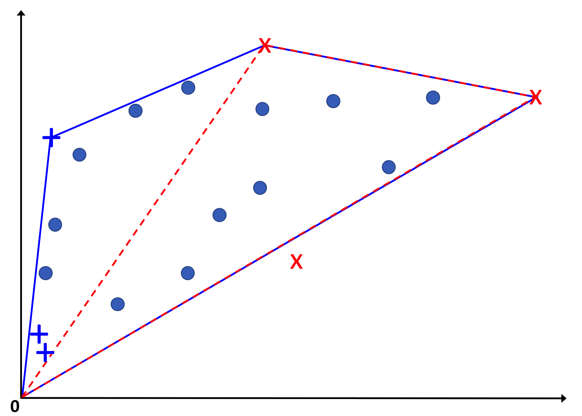
Figure 2: Example of a bilinear mixing for which SNPALQ is successful at recovering $\mathbf{W}$ but SNPA is not (the principle is the same for LQ, except that there are more virtual sources). There are three primary sources, represented with the red X markers, and three virtual sources, namely $\mathbf{w}_{i}\odot\mathbf{w}_{j}$ for $i\neq j$ and $1\leq i,j\leq 3$, represented with the blue $+$ markers. The columns of $\bar{\mathbf{X}}$ are made of the primary sources and the mixed points represented with the blue circles. The red dashed line is the convex hull of the origin and the sources extracted after two iterations of SNPA. The plain blue line is the convex hull of the origin and the sources extracted by SNPALQ after two iterations, as well as the corresponding virtual source. Only the last primary source lies outside of the blue convex hull. Therefore, SNPALQ extracts it in its third iteration and then stops, returning the primary sources only. On the other hand, at the third iteration, SNPA fails to extract the last primary source because some of the (mixed) columns of $\bar{\mathbf{X}}$ lie further away from the red dashed convex hull. Moreover, it will need in total 8 iterations to terminate because the convex hull of the columns of $\bar{\mathbf{X}}$ has 8 vertices (we assume the virtual sources do not appear purely in the data set).

SNPALQ will be proved in Section LABEL:sec:robustness_SNPAB to extract the primary sources in the first $r$ steps, under specific conditions. SNPALQ alternates the two above steps until one of the following two criteria is met:

• A maximum of $r_{\text{max}}$ columns have been extracted. If an upper bound is not available, one can take $r_{\text{max}}=n$ so that SNPALQ relies on the second stopping criterion only. Our theoretical results will rely on this criterion assuming $r$ is know.

• $\left\|{\mathbf{R}}\right\|_{F}\leq t\left\|{\bar{\mathbf{X}}}\right\|_{F}$: the algorithm stops when the relative reconstruction error is sufficiently small. The choice of a good value for the tolerance parameter $t$ is important: if $t$ is too large, the SNPALQ could stop before the extraction of all the sources. If $t$ is too low, the SNPALQ could extract too many source candidates in the presence of noise, making the whole algorithm computationally expensive. Theoretical results concerning the choice of $t$ are left for future work.

Algorithm 1 Successive Nonnegative Projection Algorithm for LQ mixtures (SNPALQ)

1:  Input: $\bar{\mathbf{X}}\in\mathbb{R}^{m\times\tilde{r}}$: a $r$-LQ $r$-near-separable matrix following Definition 1.1 and Constraints (4), $f$: a strongly convex function satisfying Assumption 2, $r_{\text{max}}$: number of sources, $t\geq 0$: stopping criterion on the norm of the residual.

1:  

2:  Initialization: $\mathbf{R}=\bar{\mathbf{X}}$, $\mathcal{K}=\{\}$, $k=1$

2:  

3:  while $\frac{\left\|{\mathbf{R}}\right\|_{F}}{\left\|{\bar{\mathbf{X}}}\right\|_{F}}>t$ and $k\leq r_{\text{max}}$ do

4:     $p=\operatorname*{argmax}_{j\in[\![n]\!]}f(\mathbf{r}_{j})$;

5:     $\mathcal{K}=\mathcal{K}\cup\{p\}$;

6:     for $j\in[\![n]\!]$ do

7:        $\mathbf{h}_{j}=\operatorname*{argmin}_{\mathbf{h}\in\Delta^{\frac{|\mathcal{K}|(|\mathcal{K}|+3)}{2}}}f(\bar{\mathbf{x}}_{j}-\Pi_{2}(\bar{\mathbf{X}}_{\mathcal{K}})\mathbf{h})$

8:        $\mathbf{r}_{j}=\bar{\mathbf{x}}_{j}-\Pi_{2}(\bar{\mathbf{X}}_{\mathcal{K}})\mathbf{h}_{j}$

9:     end for

10:     $k=k+1$

11:  end while

11:  

12:  Output: A set $\mathcal{K}$ of indices such that $\bar{\mathbf{X}}_{\mathcal{K}}\simeq\mathbf{W}$ up to a permutation.

2.2 Brute force algorithm

The conditions ensuring SNPALQ to recover the sources might not be satisfied in practice (see Sections LABEL:sec:interp_SNPALQ and LABEL:sec:exp_cond). Therefore, we propose here a second algorithm, BF, inspired by the algorithm of Arora et al. [Arora2016] for linear mixtures. As we will see in Section LABEL:sec:robustness_postProc, it requires milder assumptions for the source recovery.

Noise-free mixtures – For the sake of simplicity, the rationale underlying BF is first exposed in the absence of noise. Let us assume w.l.o.g. that there are no duplicated columns in the data set $\mathbf{X}$. Due to the separable assumption, $\mathbf{X}$ can be written as:

(5) $$\mathbf{X}=\left[\mathbf{W},\tilde{\mathbf{X}}\right]\mathbf{P}\;\in\;\mathbb{R}^{m\times n},$$

where $\mathbf{P}$ is a permutation and $\tilde{\mathbf{X}}$ contains the LQ mixings of $\mathbf{W}$. Let us consider a column of $\mathbf{X}$, $\mathbf{x}_{k}$ for $k\in[\![n]\!]$. We can check whether it is contained in the convex hull of the other columns of $\mathbf{X}$, their LQ mixtures and the origin by solving

$$s_{k}\;=\;\min_{\mathbf{h}\in\Delta^{\frac{n(n+3)}{2}-1}}\left\|{\mathbf{x}_{k}-\Pi_{2}(\mathbf{X})_{\setminus\{k\}}\mathbf{h}}\right\|_{2}.$$

If $\mathbf{x}_{k}$ is not a column of $\mathbf{W}$, we have $s_{k}=0$ under the $r$-LQ separable mixing model (Definition 1.1 with $\mathbf{N}=0$). Moreover, under the assumption that $\mathbf{W}$ is order-2 $\alpha$-robust simplicial, that is, $\alpha_{2}(\mathbf{W})>0$, $\mathbf{x}_{k}$ is a source, that is, a column of $\mathbf{W}$, if and only if $s_{k}>0$.

For sake of consistency with SNPALQ, this condition can be generalized to any function $f$ fulfilling Assumption 2. Adopting this generalization, $\mathbf{x}_{k}$ is as primary source if and only if

(6) $$\min_{\mathbf{h}\in\Delta^{\frac{n(n+3)}{2}-1}}f\left(\mathbf{x}_{k}-\Pi_{2}(\mathbf{X})_{\setminus\{k\}}\mathbf{h}\right)>0.$$

Noisy mixtures – We here extend the above principles to make the BF algorithm able to recover an approximation of $\mathbf{W}$ from noisy mixtures $\bar{\mathbf{X}}={\mathbf{X}}+{\mathbf{N}}$ for a bounded noise fulfilling $\max_{i\in[\![t]\!]}\left\|{\mathbf{n}_{i}}\right\|_{2}\leq\epsilon$ for some $\epsilon\geq 0$; see Algorithm 2. To do so, we need to modify (6) in two ways.

• In the noise-free case, we assumed that no duplicated columns are present within $\mathbf{X}$, and it is easy to discard such duplicates. In the noisy setting, when evaluating the residual (6), not only the column $\bar{\mathbf{x}}_{k}$ should be removed from $\Pi_{2}(\bar{\mathbf{X}})$ but also all columns close to $\bar{\mathbf{x}}_{k}$ (see Figure 3 for an illustration).

  

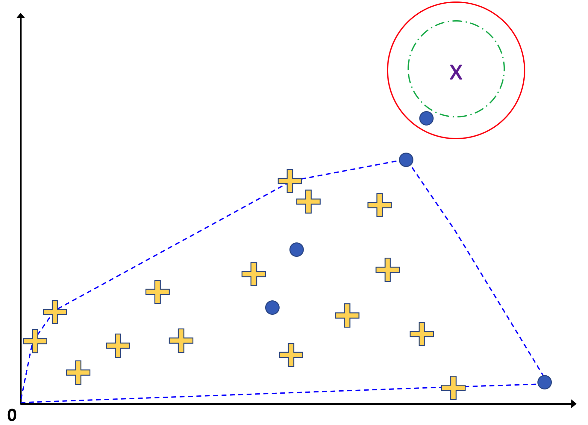
  (a)

  

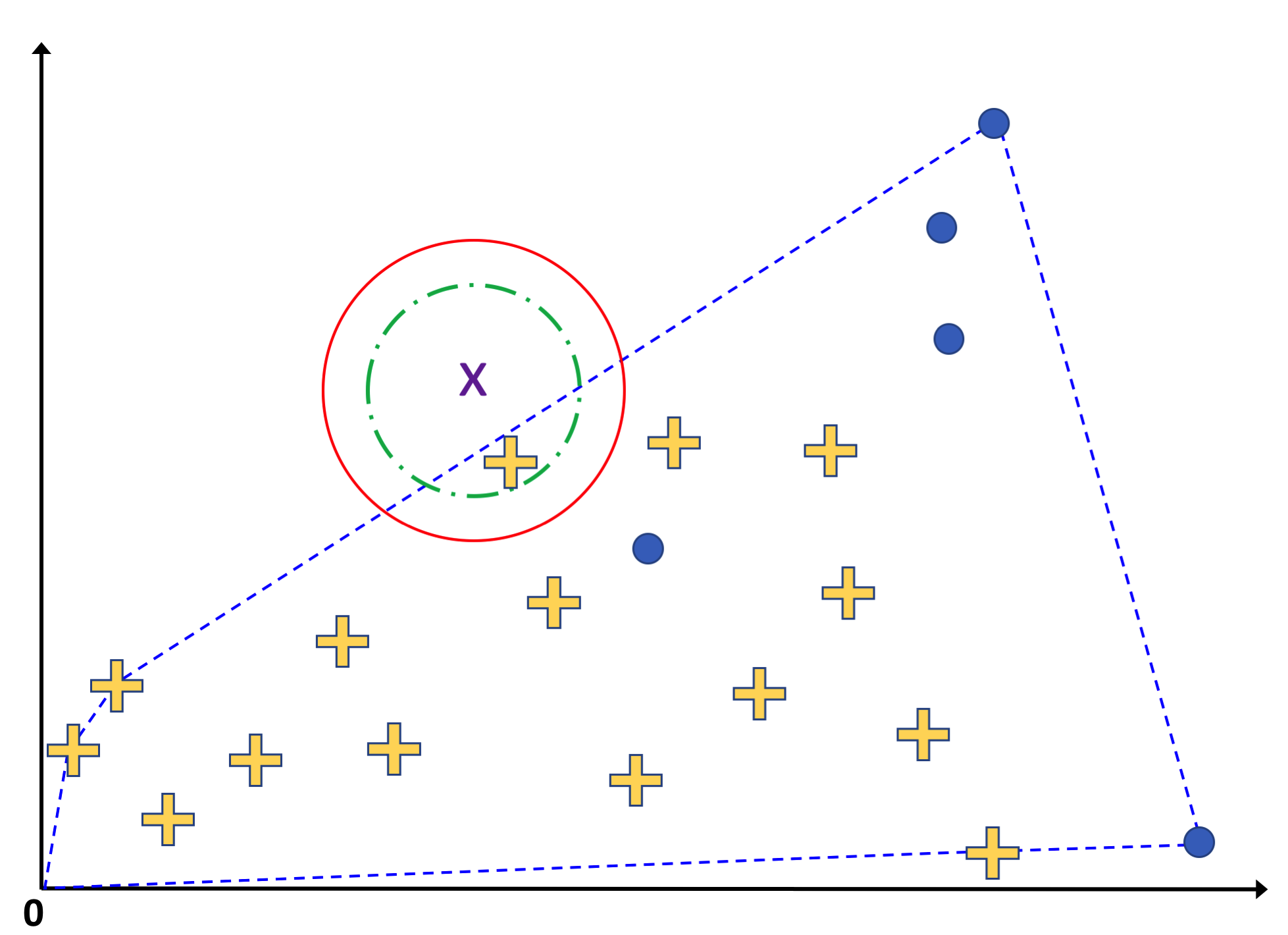
  (b)

  

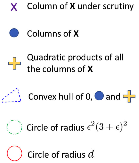
  Figure 3: Illustration of condition (7) with $f(\cdot)=\left\|{\cdot}\right\|_{2}$. The point under scrutiny $\bar{\mathbf{x}}_{k}$ is represented in violet (’X’ marker). The dots are the columns of $\mathbf{X}{\setminus\{k\}}$, and the yellow cross (’+’ marker) correspond to the quadratic products of the columns of $\mathbf{X}$. The plain line ball of radius $d$ and center $\bar{\mathbf{x}}_{k}$ contains the columns of $\bar{\mathbf{X}}$ which are discarded in (7). The dotted polygon is the convex hull of the origin and the columns of $\Pi_{2}(\mathbf{X})_{\setminus\{k\}}$ that are not contained in the ball of radius $d$ around $\bar{\mathbf{x}}_{k}$. The dashed circle of radius $\epsilon^{2}(3+\epsilon)^{2}$ indicates the distance at which the point must be located from the dotted convex hull to be considered an LQ-robust loner. On the figure (a), the dashed circle does not intersect the convex hull, and hence the cross is an LQ-robust loner. On figure (b), the dashed circle overlaps the convex hull, making that its center point is not a robust loner.

• Moreover, as the noise might shift mixed data points outside the convex hull formed by $\Pi_{2}(\mathbf{W})$ and the origin, $s_{k}$ might be nonzero for a mixed column $\bar{\mathbf{x}}$ (that is, $\bar{\mathbf{x}}_{k}=\tilde{\mathbf{x}}_{j}$ for some $j\in[\![n-r]\!]$); see Figure 3 for an illustration.

Therefore, the condition (6) in the noiseless case should be modified to

(7) $$\min_{\mathbf{h}\in\Delta^{\frac{n(n+3)}{2}-1}}f\left(\bar{\mathbf{x}}_{k}-\Pi_{2}(\bar{\mathbf{X}})_{\setminus\{i\in[\![n]\!]\ |\ f\left(\bar{\mathbf{x}}_{i}-\bar{\mathbf{x}}_{k}\right)>d\}}\mathbf{h}^{*}\right)>\frac{L}{2}\epsilon^{2}(3+\epsilon)^{2},$$

with $L$ the Lipschitz constant of $f$ and $d$ a threshold parameter discussed in Appendix LABEL:sec:proofs; see (LABEL:eq:d) for an explicit value. The right-hand side stems from the fact that the noise is corrupting both the data columns (with a maximum energy of $\epsilon$) and their quadratic products (with a maximum energy of $2\epsilon+\epsilon^{2}$ if the columns of $\mathbf{X}$ have a unit norm); see Definition LABEL:def:robust_loner_full.

Following [Arora2016], the columns of $\bar{\mathbf{X}}$ satisfying the condition (7) are called the LQ-robust loners. Section LABEL:sec:robustness_postProc will show that these columns exactly correspond to good approximations of the sources. To approximately recover the sources, the BF algorithm then amounts to check which columns of $\bar{\mathbf{X}}$ are LQ-robust loners. However, due to the noise, different LQ-robust loners may be candidates for estimating the same source. Therefore, at the end of BF, the LQ-robust loners need to be clustered to obtain a single estimate of each source. Fortunately, such a clustering – described in Algorithm 2 – is easy and does not lead to any indeterminacy as the LQ-robust loners are located close to the sources, which are comparatively further from each others.

Algorithm 2 Brute force (BF)

1:  Input: A $r$-LQ $r$-near-separable matrix $\bar{\mathbf{X}}\in\mathbb{R}^{m\times\tilde{r}}$ following Definition 1.1 and constraints (Eq. 4), $r$: number of sources, and $f$ a strongly convex function satisfying Assumption 2, $\epsilon=\max_{i\in[\![t]\!]}\left\|{\mathbf{n}_{i}}\right\|_{2}$, $d$ given by Equation (LABEL:eq:d).

1:  

2:  Initialization: $\mathcal{K}=\{\}$

2:  

3:  for $k\in[\![t]\!]$ do

4:     $\mathbf{h}_{k}=\operatorname*{argmin}_{\mathbf{h}\in\Delta}f\left(\bar{\mathbf{x}}_{k}-\Pi_{2}(\bar{\mathbf{X}})_{\setminus\{i\in[\![t]\!]\ |\ f(\bar{\mathbf{x}}_{i}-\bar{\mathbf{x}}_{k})>d\}}\mathbf{h}\right)$

5:     if $f\left(\bar{\mathbf{x}}_{k}-\Pi_{2}(\bar{\mathbf{X}}_{\mathcal{N}})_{\setminus\{i\in[\![t]\!]\ |\ f(\bar{\mathbf{x}}_{i}-\bar{\mathbf{x}}_{k})>d\}}\mathbf{h}_{k}\right)>\frac{L}{2}\epsilon^{2}(3+\epsilon)^{2}$ then

6:        $\mathcal{K}=\mathcal{K}\cup\{k\}$

7:     end if

8:  end for

8:  

9:  Clustering on $\bar{\mathbf{X}}_{\mathcal{K}}$: assign two columns $\bar{\mathbf{x}}_{i}$ and $\bar{\mathbf{x}}_{j}$ of $\bar{\mathbf{X}}_{\mathcal{K}}$ to the same cluster if and only if $\left\|{\bar{\mathbf{x}}_{j}-\bar{\mathbf{x}}_{k}}\right\|_{2}\leq 2\sqrt{\frac{2}{\mu}(d+\epsilon L(2K(\mathbf{X})+\epsilon))}$. Update $\mathcal{K}$ by keeping only one column for each cluster.

9:  

10:  Output: A set $\mathcal{K}$ of indices such that $\bar{\mathbf{X}}_{\mathcal{K}}\simeq\mathbf{W}$ up to a permutation.

BF algorithm as a post-processing – Even if the BF algorithm can be used per se to perform separation from LQ near-separable mixtures, it can also serve as a post-processing to refine the results provided by SNPALQ. This strategy is particularly appealing when SNPALQ robustness conditions are not met, in which case SNPALQ may extract mixed data columns or virtual sources in addition to the sought-after primary sources. Given an SNPALQ solution $\bar{\mathbf{X}}_{\mathcal{K}}$, assume $r$ columns correspond to the primary sources $\mathbf{W}$, and the $|\mathcal{K}|-r$ remaining ones to (spurious) columns in which the primary sources are mixed along with their quadratic products. Up to a permutation, the SNPALQ solution can be written as

(8) $$\bar{\mathbf{X}}_{\mathcal{K}}\simeq\left[\mathbf{W},\tilde{\mathbf{X}}\right]\in\mathbb{R}^{m\times|\mathcal{K}|},$$

where $P$ is a permutation, and $\tilde{\mathbf{X}}\in\mathbb{R}^{m\times(|\mathcal{K}|-r)}$ are data points. This matches the form of (5). Therefore, instead of using the BF algorithm directly on the data set $\bar{\mathbf{X}}$, it can be applied on the SNPALQ solution $\bar{\mathbf{X}}_{\mathcal{K}}$, which has in practice a significantly smaller number of columns, that is, $|\mathcal{K}|\ll n$. Using BF as a post-processing step significantly reduces the computational cost; see Section LABEL:sec:complexity. Furthermore, it is worth noting that SNPALQ already identifies as sources columns of $\bar{\mathbf{X}}$ lying far from each other. Thus, in our experiments, the clustering step in BF, whenever used as a post-processing, was never necessary since each cluster contained exactly one point.