ADCME: Learning Spatially-varying Physical Fields using Deep Neural Networks

Abstract

ADCME is a novel computational framework to solve inverse problems involving physical simulations and deep neural networks (DNNs). This paper benchmarks its capability to learn spatially-varying physical fields using DNNs. We demonstrate that our approach has superior accuracy compared to the discretization approach on a variety of problems, linear or nonlinear, static or dynamic. Technically, we formulate our inverse problem as a PDE-constrained optimization problem. We express both the numerical simulations and DNNs using computational graphs and therefore, we can calculate the gradients using reverse-mode automatic differentiation. We apply a physics constrained learning algorithm (PCL) to efficiently back-propagate gradients through iterative solvers for nonlinear equations. The open source software which accompanies the present paper can be found at

https://github.com/kailaix/ADCME.jl

1 Introduction

Inverse problems in computational engineering aim at learning physical parameters or spatially-varying fields from observations. These observations are usually the partial output of physical models, typically described by partial differential equations (PDEs). There is a vast array of literature covering inverse problems with an unknown spatially-varying field in geophysics [1, 2, 3, 4], fluid dynamics [5, 6], electromagnetism [7], etc. In these applications, observations are indirect in the sense that they are not pointwise values of the unknown field. A standard approach is to discretize the spatially-varying field on the grid points, which is the same as our computational grid, and estimate pointwise values from observations. However, this approach is usually ill-posed when the dataset is small, which is common due to expensive and challenging experiments or measurements [8, 9].

Deep neural networks (DNN) are an effective approach to provide an expressive functional form for physical applications [10, 11]. It also provides some appropriate regularization to the optimization problem via proper initialization and choices of architectures [12, 13, 14, 15]. In this paper, we present the capability of ADCME for learning spatially-varying physical parameters using deep neural networks [16, 17, 18]. In our approach, the inverse problem is formulated as a PDE-constrained optimization problem [19, 20, 21, 22]

$$\min_{\theta}\;J(u)\quad\text{($u$ is indirectly a function of $\theta$), \quad such that}\;F(u,\mathcal{N}_{\theta})=0$$

Here $u$ is the state variable, $F$ is the PDE constraint, and $\mathcal{N}_{\theta}(\mathbf{x})$ is the approximation of the unknown field ($\mathbf{x}$ is the coordinate). The numerical solution $u$ can be formally expressed as a function of $\theta$ and we arrive at an unconstrained optimization problem by plugging $u(\theta)$ into $J(u)$ (see Figure 1)

$$\min_{\theta}\;L(\theta):=J(u(\theta))$$ (1)

Figure 1: Coupling a deep neural network and a numerical PDE solver.

A gradient-based optimization algorithm is used to solve Eq. 1. The major challenge is to calculate $\nabla_{\theta}L(\theta)$. To this end, we express both numerical simulators (e.g., finite element methods) and deep neural networks as computational graphs. The advantage of this approach is that once we implement the forward computation, the gradient can be calculated using reverse-mode automatic differentiation (AD) [23, 24, 25], which is equivalent to the so-called discrete adjoint methods [26, 27, 28] for PDE solvers. ADCME provides a framework for implementing numerical schemes as computational graphs and incorporating deep neural networks. The computational graph operates on tensor operation (e.g., linear solvers) or higher levels (e.g., finite element assembling); with such task granularity, we enjoy a good balance between performance overhead from AD (e.g., reducing memory demands by checkpointing schemes for certain operators) and development efforts.

Note that numerical simulators in ADCME are intrinsically different from traditional simulators: in ADCME, numerical simulators are defined by specifying the dependency of many individual and reusable operators, and these operators are equipped with gradient-backpropagation capabilities with the implementation of efficient adjoint state methods (possibly with checkpointing schemes for saving memories).

With the advent of experimental techniques that enable gathering large amounts of data inexpensively, we anticipate that modeling using deep neural networks will become essential tools for data-driven discovery. As a result, developing software platforms with AD capabilities that can be coupled with sophisticated optimizers can be expected to have great impact on computational engineering.

2 Mathematical Model

Let us consider the Stokes problem as a concrete example. The governing equations for the Stokes problem are [29]

$$-\nabla\cdot(\nu\nabla u)+\nabla p=f\text{ in }\Omega$$ (2)

$$\nabla\cdot u=0\text{ in }\Omega,\qquad u=0\text{ on }\partial\Omega$$

Here $u:\mathbb{R}^{2}\rightarrow\mathbb{R}^{2}$, $p:\mathbb{R}^{2}\rightarrow\mathbb{R}$ are state variables; $\nu(\mathbf{x})$ denotes the spatially-varying fluid viscosity, which we want to estimate from observations of $u$ or $p$; $\Omega\subset\mathbb{R}^{2}$ is the computational domain, and $f\in[L^{2}(\Omega)]^{2}$ is the unit external volumetric force. We approximate $\nu(\mathbf{x})$ with a deep neural network $\nu_{\theta}(\mathbf{x})$, which maps the coordinate $\mathbf{x}$ to a scalar value. $\theta$ are the DNN weights and biases.

Another approach is to discretize $\nu(\mathbf{x})$ at the Gauss quadrature points or in each finite element because only the values at Gauss quadrature points are used in the assembling procedures. Therefore, we have a vector of unknowns $\{\nu(\mathbf{x}_{k})\}$, where $\{\mathbf{x}_{k}\}$ is the collection of all Gauss quadrature points of all the elements. To reduce the number of degrees of freedoms, we can also consider a piecewise constant function where $\nu$ is a constant on each element.

The weak formulation of the Stokes equation finds $u\in[H^{1}_{0}(\Omega)]^{2}$ and $p\in L_{0}^{2}(\Omega)$ satisfying

$$(\nabla u,\nu_{\theta}\nabla v)-(\nabla\cdot v,p) =(f,v), v\in[H^{1}_{0}(\Omega)]^{2}$$ (3)

$$(\nabla\cdot u,q) =0, q\in L_{0}^{2}(\Omega)$$

The finite element formulation using a P2/P0 (a quadratic velocity space and a pressure space of piecewise constant) element leads to the linear system

$$\begin{bmatrix}A(\theta)&-B\\ B^{T}&0\end{bmatrix}\begin{bmatrix}U\\ P\end{bmatrix}=\begin{bmatrix}F_{1}\\ F_{2}\end{bmatrix}$$

Note that the entries of $A$ are a function of $\theta$. In ADCME, constructing DNNs and assembling procedures of $A$, $B$, $F_{1}$, and $F_{2}$ are treated as nodes in the computational graph. These procedures are capable of back-propagating the gradients from downstream operators of the computational graph to upstream ones. When the forward computation is defined, a computational graph is constructed implicitly.

The numerical scheme is used to compute the discrete solution $U$ and $P$, and we use $(U,P)$ to compute a loss function. Because we have constructed a computational graph, we are able to calculate the gradients by reverse-mode AD. One challenge here is that the numerical PDE solver may be nonlinear, leading to the solution of an implicit equation. To efficiently back-propagate the gradients, we apply the physics constrained learning method (PCL) proposed in [30] to extract the gradients. The core idea is to use the implicit function theorem to implement the adjoint rule [31, 32].

3 Numerical Experiments

In this section, numerical examples, which cover linear and nonlinear elasticity, Stokes problems, and Burgers’ equations, are presented to verify the effectiveness of our approach. We consider both a regular domain (square) and an irregular domain (a plate with two holes). The hyperelasticity problem involves nonlinearity in the numerical solver, and the Burgers’ equation involves both nonlinearity and time stepping. As for numerical methods, the finite element method is used. For simplicity, the observations are all discrete solutions of the state variables unless specified. The neural network is a fully-connected deep neural network with 20 neurons per layer and 3 hidden layers. The activation function is tanh. We use the L-BFGS-B optimizer [33] with full batches.

In what follows, we mention briefly our findings and the details of the numerical results can be found in the appendix. We will compare two approaches. The “discretization” methods assume that the values of $\nu(\mathbf{x}_{k})$ can be optimized independently. Using our previous notations, we define $\theta=\{\nu(\mathbf{x}_{k})\}_{k}$ for all Gauss quadrature points $\mathbf{x}_{k}$. We also show benchmarks where $\nu(\mathbf{x})$ is approximated by a constant inside each element and we may write $\theta=\{\nu(\mathbf{x}_{e})\}_{e}$ where $e$ is now an element. The second approach represents the unknown function using a DNN.

We found that for discretization methods, the optimizer often leads to nonphysical solutions, i.e., values at some point are too large or negative, and this anomaly ends up breaking the numerical simulator. For DNNs, we do not impose extra constraints on the outputs except that we add a small positive values to the last layer to ensure DNNs start from a reasonable initial guess. Still, DNNs lead to a physical solution that is close to the exact solution. In summary, DNNs were found to be more stable and accurate than the discretization approaches in our problems.

3.1 Linear Elasticity

We consider the static linear elasticity problem on a unit square [34], where we have a spatially-varying Young’s modulus $E(\mathbf{x})$ and a Poisson’s ratio $\nu=0.3$. The governing equation for the linear elasticity problem is

$$\sigma_{ij,j}+b_{i}=0,\quad\varepsilon_{ij}=\frac{1}{2}(u_{j,i}+u_{i,j}),\quad x\in\Omega$$ (4)

$$\sigma_{ij}=\lambda\delta_{ij}\varepsilon_{kk}+\mu(\varepsilon_{ij}+\varepsilon_{ji}),\quad x\in\Omega$$

$$\sigma_{ij}n_{j}=t_{j},\quad x\in\Gamma_{N};\quad u_{i}=(u_{0})_{i},\ x\in\Gamma_{D}$$

$$\lambda=\frac{E\nu}{(1+\nu)(1-2\nu)},\quad\mu=\frac{E\nu}{1-\nu^{2}}$$

Here $\sigma_{ij}$ is the stress tensor, $b_{i}$ is the body force, $u_{i}$ is the displacement, $\Gamma_{N}\cap\Gamma_{D}=\emptyset,\ \partial\Omega=\Gamma_{N}\cup\Gamma_{D}$.

We approximate $E(\mathbf{x})$ using a deep neural network. The results are shown in Figure 2. As a comparison, we also show results where we represent $E(\mathbf{x})$ as a discrete vector of trainable variables. We call this the “discretization” approach. We found that it did not work without imposing constraints on the trainable variables. In our experiment, the trainable variables were transformed from $E_{i}$ to $|E_{i}|$ (positivity constraint), where $E_{i}$ is the estimated $E(\mathbf{x})$ on the $i$-th Gauss points. Despite this, we can see that the DNN approach provides a better result that the discretization approach.

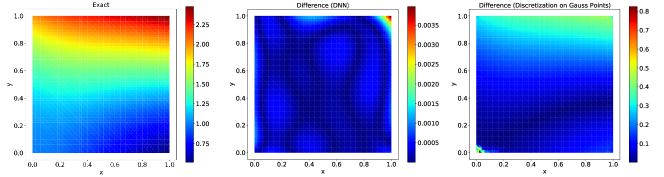
Figure 2: Convergence result for the static linear elasticity problem after 10,000 iterations. For the discretization methods, we see we have some large errors at the lower left corner and top right region, and these anomalies break the numerical solver. The optimizer stops after 981 iterations. Note that the scales for the second and third plots are different.

3.2 Stokes Problem

The next problem considered is the Stokes problem Eq. 2. The finite element formulation of the Stokes problem leads to a linear system, but has an extra pressure field compared to the linear elasticity problem. We assume that only the pressure field is known and we use this information to solve inverse problem.

We make $\nu(\mathbf{x})$ a spatially-varying field. We were not able to obtain convergence result using the discretization approach even after imposing bound constraints on the trainable variables. This indicates that the inverse problem is quite ill-conditioned. The result for DNN is shown in Figure 3.

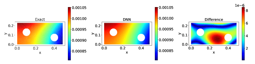
Figure 3: Convergence result for the Stokes problem after 600 iterations. For the discretization methods, the estimation did not converge to the correct results.

3.3 Hyperelasticity

The hyperelasticity problem can be described as an energy-minimization problem. We consider a common neo-Hookean energy model [35] and assume that the Young’s modulus $E(\mathbf{x})$ is a spatially-varying unknown field. The Lamé parameters are defined by the Young’s modulus $E$ and Poisson ration $\nu$:

$$\lambda=\frac{E\nu}{(1+\nu)(1-2\nu)},\quad\mu=\frac{E}{2(1+\nu)}$$

Using the finite element method to solve the energy-minimization problem leads to a nonlinear equation. The forward computation typically involves a Newton-Raphson iteration. To back-propagate the gradient through the nonlinear numerical solver, we applied the physics constrained learning to the Newton-Raphson solver.

We let the Young’s modulus $E(\mathbf{x})$ be an unknown spatially-varying field. Figure 4 shows the result. We see for this problem, the discretization approach provides an estimate that is close to the exact solution, and the corresponding loss function decays much faster than DNNs. However, the learned $E(\mathbf{x})$ field is not as smooth as DNNs and the maximum pointwise absolute error is much larger than DNNs.

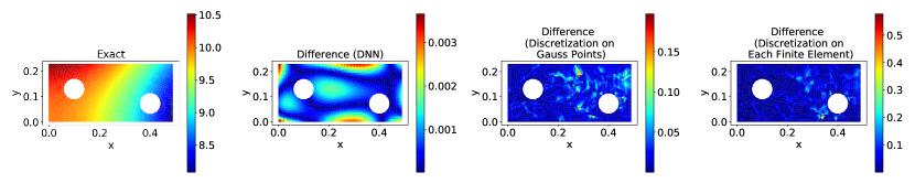
Figure 4: Convergence result for the hyperelasticity problem after 10,000 iterations. For the discretization method with piecewise constants, we use the prediction obtained at the 2,740th iteration, at which point the optimizer terminated.

3.4 Burgers’ Equation

The final example aims to demonstrate the capability of our algorithm for solving time-dependent nonlinear problems. We consider the Burgers’ equation [36] with a spatially-varying viscosity parameter $\nu(\mathbf{x})$.

We use the finite element method to discretize the Burgers’ equation spatially and apply an implicit time integrator. This results in a time marching scheme, in which a nonlinear equation needs to be solved in each iteration. The physics constrained learning is used to solve the nonlinear equation.

We make $\nu(\mathbf{x})$ a spatially-varying field and apply both the DNN and the discretization approach to learn the physical field. The result is shown in Figure 5. Due to the ill-posedness of the inverse problem and lack of spatial correlation for the discretized $\nu$, we were not able to obtain convergence result with the discretization approach if we use a constant initial guess. To this end, we initialize the discretization using a field that is close to the exact field. Even with this impractical approach, the estimation is not as accurate as DNNs.

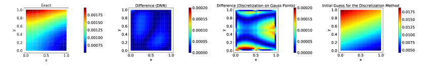
Figure 5: Convergence result for the Burgers’ equation after 60 iterations (DNN) and 16 iterations (the Discretization Method). The optimization terminates at these iterations due to satisfying the stopping criterion.

4 Conclusion

We have presented the capability of ADCME for learning spatially-varying physical parameters using deep neural networks. We showed that the DNN approach gives us a much more accurate solution compared to the traditional discretization approach in the small data regime. In our approach, both numerical simulators and deep neural networks are expressed as computational graphs, and thus gradients can be back-propagated algorithmically once the forward computation is implemented. Particularly, for nonlinear solvers, we apply the physics constrained learning approach to back-propagate the gradients. The preliminary results on several PDE examples demonstrate the effectiveness of our approach. Note that the present work relies on an optimizer for a highly nonconvex problem and the well-posedness of the optimization problem, both of which remain elusive. We plan to investigate this direction further and develop a diagnosis toolbox in the future.

Broader Impact

This work allows developing more accurate mathematical models based on experimental data or based on a model developed at a finer scale (e.g., molecular scale). Advances in this paper will enable cheaper and more accurate computational models for a broad range of engineering and scientific applications. Computer simulations of engineering and physical systems are keys in many areas, including optimization, control, imaging, and failure analysis. Developing sophisticated computer models allows making accurate predictions for complex systems without having to resort to expensive experiments. Advances in sciences and engineering have a wide range of impacts on society, which are, for the most part, positive, such as transportation, energy, communication, and medicine, but, in some cases, may be harmful such as pollution and global warming or when applied to the development and production of weapons.

References

- [1] Jorge Luis Landa, Dhananjay Kumar, et al. Joint inversion of 4D seismic and production data. In SPE annual technical conference and exhibition. Society of Petroleum Engineers, 2011.
- [2] Mrinal K Sen and Paul L Stoffa. Global optimization methods in geophysical inversion. Cambridge University Press, 2013.
- [3] Weiqiang Zhu, Kailai Xu, Eric Darve, and Gregory C Beroza. A general approach to seismic inversion with automatic differentiation. arXiv preprint arXiv:2003.06027, 2020.
- [4] Dongzhuo Li, Kailai Xu, Jerry M Harris, and Eric Darve. Coupled time-lapse full-waveform inversion for subsurface flow problems using intrusive automatic differentiation. Water Resources Research, 56(8):e2019WR027032, 2020.
- [5] Anand Pratap Singh and Karthik Duraisamy. Using field inversion to quantify functional errors in turbulence closures. Physics of Fluids, 28(4):045110, 2016.
- [6] Eric J Parish and Karthik Duraisamy. A paradigm for data-driven predictive modeling using field inversion and machine learning. Journal of Computational Physics, 305:758–774, 2016.
- [7] Anna Kelbert, Naser Meqbel, Gary D Egbert, and Kush Tandon. ModEM: A modular system for inversion of electromagnetic geophysical data. Computers & Geosciences, 66:40–53, 2014.
- [8] Sergey Fomel. Shaping regularization in geophysical-estimation problems. Geophysics, 72(2):R29–R36, 2007.
- [9] Daniel Z Huang, Kailai Xu, Charbel Farhat, and Eric Darve. Learning constitutive relations from indirect observations using deep neural networks. Journal of Computational Physics, page 109491, 2020.
- [10] Aaditya Chandrasekhar and Krishnan Suresh. TOuNN: Topology optimization using neural networks. Structural and Multidisciplinary Optimization (accepted, 2020.
- [11] Stephan Hoyer, Jascha Sohl-Dickstein, and Sam Greydanus. Neural reparameterization improves structural optimization. arXiv preprint arXiv:1909.04240, 2019.
- [12] Maziar Raissi, Paris Perdikaris, and George E Karniadakis. Physics-informed neural networks: A deep learning framework for solving forward and inverse problems involving nonlinear partial differential equations. Journal of Computational Physics, 378:686–707, 2019.
- [13] Boris Hanin and David Rolnick. How to start training: The effect of initialization and architecture. In Advances in Neural Information Processing Systems, pages 571–581, 2018.
- [14] Kailai Xu and Eric Darve. The neural network approach to inverse problems in differential equations. arXiv preprint arXiv:1901.07758, 2019.
- [15] Kailai Xu, Daniel Z Huang, and Eric Darve. Learning constitutive relations using symmetric positive definite neural networks. arXiv preprint arXiv:2004.00265, 2020.
- [16] Dmitry Ulyanov, Andrea Vedaldi, and Victor Lempitsky. Deep image prior. In Proceedings of the IEEE Conference on Computer Vision and Pattern Recognition, pages 9446–9454, 2018.
- [17] JH Rick Chang, Chun-Liang Li, Barnabas Poczos, BVK Vijaya Kumar, and Aswin C Sankaranarayanan. One network to solve them all–solving linear inverse problems using deep projection models. In Proceedings of the IEEE International Conference on Computer Vision, pages 5888–5897, 2017.
- [18] Tiffany Fan, Kailai Xu, Jay Pathak, and Eric Darve. Solving inverse problems in steady state navier-stokes equations using deep neural networks. arXiv preprint arXiv:2008.13074, 2020.
- [19] Lorenz T Biegler, Omar Ghattas, Matthias Heinkenschloss, and Bart van Bloemen Waanders. Large-scale PDE-constrained optimization: an introduction. In Large-Scale PDE-Constrained Optimization, pages 3–13. Springer, 2003.
- [20] Tyrone Rees, H Sue Dollar, and Andrew J Wathen. Optimal solvers for PDE-constrained optimization. SIAM Journal on Scientific Computing, 32(1):271–298, 2010.
- [21] Juan Carlos De los Reyes. Numerical PDE-constrained optimization. Springer, 2015.
- [22] Roland Herzog and Karl Kunisch. Algorithms for PDE-constrained optimization. GAMM-Mitteilungen, 33(2):163–176, 2010.
- [23] Atılım Günes Baydin, Barak A Pearlmutter, Alexey Andreyevich Radul, and Jeffrey Mark Siskind. Automatic differentiation in machine learning: a survey. The Journal of Machine Learning Research, 18(1):5595–5637, 2017.
- [24] Adam Paszke, Sam Gross, Soumith Chintala, Gregory Chanan, Edward Yang, Zachary DeVito, Zeming Lin, Alban Desmaison, Luca Antiga, and Adam Lerer. Automatic differentiation in PyTorch. 2017.
- [25] Martín Abadi, Paul Barham, Jianmin Chen, Zhifeng Chen, Andy Davis, Jeffrey Dean, Matthieu Devin, Sanjay Ghemawat, Geoffrey Irving, Michael Isard, et al. Tensorflow: A system for large-scale machine learning. In 12th USENIX symposium on operating systems design and implementation (OSDI 16), pages 265–283, 2016.
- [26] R-E Plessix. A review of the adjoint-state method for computing the gradient of a functional with geophysical applications. Geophysical Journal International, 167(2):495–503, 2006.
- [27] Karin Nachbagauer, Stefan Oberpeilsteiner, Karim Sherif, and Wolfgang Steiner. The use of the adjoint method for solving typical optimization problems in multibody dynamics. Journal of Computational and Nonlinear Dynamics, 10(6), 2015.
- [28] Antoine McNamara, Adrien Treuille, Zoran Popović, and Jos Stam. Fluid control using the adjoint method. ACM Transactions On Graphics (TOG), 23(3):449–456, 2004.
- [29] Lin Mu and Xiu Ye. A simple finite element method for the Stokes equations. Advances in Computational Mathematics, 43(6):1305–1324, 2017.
- [30] Kailai Xu and Eric Darve. Physics constrained learning for data-driven inverse modeling from sparse observations. arXiv preprint arXiv:2002.10521, 2020.
- [31] Patrick E Farrell, David A Ham, Simon W Funke, and Marie E Rognes. Automated derivation of the adjoint of high-level transient finite element programs. SIAM Journal on Scientific Computing, 35(4):C369–C393, 2013.
- [32] Kailai Xu, Alexandre M Tartakovsky, Jeff Burghardt, and Eric Darve. Inverse modeling of viscoelasticity materials using physics constrained learning. arXiv preprint arXiv:2005.04384, 2020.
- [33] Dong C Liu and Jorge Nocedal. On the limited memory bfgs method for large scale optimization. Mathematical programming, 45(1-3):503–528, 1989.
- [34] Eduardo A de Souza Neto, Djordje Peric, and David RJ Owen. Computational methods for plasticity: theory and applications. John Wiley & Sons, 2011.
- [35] Hyperelasticity — FEniCS project. https://fenicsproject.org/docs/dolfin/1.4.0/python/demo/documented/hyperelasticity/python/documentation.html. (Accessed on 09/30/2020).
- [36] Hongqing Zhu, Huazhong Shu, and Meiyu Ding. Numerical solutions of two-dimensional Burgers’ equations by discrete Adomian decomposition method. Computers & Mathematics with Applications, 60(3):840–848, 2010.
- [37] Ole Sigmund. A 99 line topology optimization code written in Matlab. Structural and multidisciplinary optimization, 21(2):120–127, 2001.