SimTreeLS: Simulating aerial and terrestrial laser scans of trees

Abstract

There are numerous emerging applications for digitizing trees using terrestrial and aerial laser scanning, particularly in the fields of agriculture and forestry. Interpretation of LiDAR point clouds is increasingly relying on data-driven methods (such as supervised machine learning) that rely on large quantities of hand-labelled data. As this data is potentially expensive to capture, and difficult to clearly visualise and label manually, a means of supplementing real LiDAR scans with simulated data is becoming a necessary step in realising the potential of these methods. We present an open source tool, SimTreeLS (Simulated Tree Laser Scans), for generating point clouds which simulate scanning with user-defined sensor, trajectory, tree shape and layout parameters. Upon simulation, material classification is kept in a pointwise fashion so leaf and woody matter are perfectly known, and unique identifiers separate individual trees, foregoing post-simulation labelling. This allows for an endless supply of procedurally generated data with similar characteristics to real LiDAR captures, which can then be used for development of data processing techniques or training of machine learning algorithms. To validate our method, we compare the characteristics of a simulated scan with a real scan using similar trees and the same sensor and trajectory parameters. Results suggest the simulated data is significantly more similar to real data than a sample-based control. We also demonstrate application of SimTreeLS on contexts beyond the real data available, simulating scans of new tree shapes, new trajectories and new layouts, with results presenting well. SimTreeLS is available as an open source resource built on publicly available libraries.

1 Introduction

LiDAR scanning is a useful tool for reality capture in various industries. In agriculture, Rosell and Sanz [2012] showed that LiDAR is considered a useful tool for rapidly capturing geometric properties of trees. Wu et al. [2020] confirmed the suitability of LiDAR from both a terrestrial and aerial context for analysing tree crop structures. Scanning allows extraction of tree parameters which are useful for growth analysis, including woody matter detection (Vicari et al. [2019], Su et al. [2019], Westling et al. [2020b]), porosity (Pfeiffer et al. [2018]), and leaf area density or distribution (Béland et al. [2011, 2014], Sanz et al. [2018]. Beyond simple tree parameters, LiDAR scanning also enables detailed investigations on real trees, like orchard mapping (Underwood et al. [2016], Reiser et al. [2018]), analysis of the light environment of a tree (Westling et al. [2018]), or historical yield analysis (Colaço et al. [2019]). Gené-Mola et al. [2019] was even able to detect fruit using intensity returns from a terrestrial LiDAR scanner, with comparable results and several advantages over vision systems. Similar applications are found in forestry, where tree geometric analysis is of interest. Tree parameters like woody matter detection (Ma et al. [2016a, b]) and Leaf Area Density (Van der Zande et al. [2011])is also of interest here, as well as further interest areas including robot navigation (Lalonde et al. [2006]) and forest inventory (Bauwens et al. [2016]). Terrestrial laser scanning is used extensively in commercial forests for plot-level inventory (Liang et al. [2016]), which is then used for validation and training for inventory over large scales based on aerial LiDAR capture (Kato et al. [2009], Wang et al. [2020], Cao et al. [2019], Almeida et al. [2019]). LaRue et al. [2020] demonstrates that aerial LiDAR captures slightly less than the terrestrial equivalent, but is well suited to macro-scales. In both industries however, LiDAR capture involves time-intensive scanning operations, and captured data can be difficult to process.

There is some value and interest for analysing trees in silico to achieve perfect digitization, generate large datasets, and perform physically challenging or destructive operations. Yang et al. [2016] and Arikapudi et al. [2015] digitized trees thoroughly for light interception analysis and geometric modelling respectively. Others have generated virtual trees using algorithmic growth (for example Functional-Structural Plant Modelling presented by White and Hanan [2012, 2016]) which allows for study of how a tree will develop using different pruning or growth decisions. Sometimes the approach is to generate computer models of particular trees, for instance Da Silva et al. [2014] and Tang et al. [2015] performed light interception efficiency analyses using computer models of apple and peach trees respectively, while Tang et al. [2019] generated virtual loquat trees to design an optimal plant canopy shape. Beyond simple computer modelling, Tao et al. [2015] used Physically Based Ray Tracing to simulate terrestrial Lidar scans, based on an approach previously used by Côté et al. [2009]. Some of these methods generate perfect data while others approximate real scanning, and both approaches have value in different application areas.

Recently, there has been a growing interest in deep learning on point clouds, as reviewed by Guo et al. [2019]. For general point cloud applications, a variety of approaches have been developed, from the multi-view convolutional neural networks presented by Su et al. [2015] to dense contextual networks Liu et al. [2019]. However, many methods primarily operate on small or perfectly sampled point clouds (Wu et al. [2015], Qi et al. [2017]), and applications on tree scans are typically neither. Kumar et al. [2019] identified trees as distinct from other object types in point clouds captured by mobile laser scanning with a total accuracy of 95.2%. In forestry, Windrim and Bryson [2018] and Xi et al. [2018] perform tree classification using fully connected 3D CNNs. In agriculture, Majeed et al. [2020] used deep learning to segment plant matter from its supporting trellis; however, typically deep learning here is applied to imagery rather than LiDAR (Bargoti et al. [2015], Apolo-Apolo et al. [2020]). A significant obstacle to deep learning on large-scale point clouds is the difficulty in acquiring large quantities of data which is labelled by human experts. Modern deep learning architectures contain potentially hundreds of thousands to millions of trainable parameters in order to make accurate and robust inference. These models demand the use of tens to hundreds of thousands of training examples to realise the potential of this complexity, and providing all of these training labels manually on real data can quickly become infeasible. LiDAR scanning must typically decide on a trade-off between quality and capture speed, with faster captures typically being more sparse or occluded and thus harder to label (Westling et al. [2020b]).

Simulation of realistic data is a viable candidate for solving the labelling issue. Many deep learning applications, in particular standard datasets and early point cloud works, use point-sampled meshes to generate point clouds on which to learn (for example, Wu et al. [2015] and Qi et al. [2017]), though this data does not realistically estimate the effect of laser scanning an object. Developing this further, Wang et al. [2019] and Goodin et al. [2019] have shown that neural networks can be trained comparably well using simulated LiDAR data. Generally in machine learning, transfer learning allows learners to minimise the required dataset by training on a similar set first, though there are complexities (Zhuang et al. [2020]). Nezafat et al. [2019] were able to transfer features learned by a pre-trained model to a different data setting, using images generated by projection of LiDAR data. This suggests that realistic simulated data which is perfectly labelled could be used to pre-train models, significantly reducing the need for manual labelling. This can also be applied to changes in setting, for instance comparing aerial to terrestrial LiDAR.

We present a software tool, SimTreeLS, to generate simulated LiDAR scans with realistic sensor parameters, trajectories and results. Other tools with similar aims have been presented like SIMLIDAR by Mendez et al. [2012], though not at the same scale or level of detail. Our approach, SimTreeLS, is specifically designed to create simulated scans of trees, for development of applications in agriculture and forestry, supports a wide variety of tree shapes and sensor types, and can be used to simulate ground-based, handheld and aerial mobile LiDAR. We present how SimTreeLS works and experimental results showing its viability as a simulated source of LiDAR data. An overview of our method is presented in Figure 1.

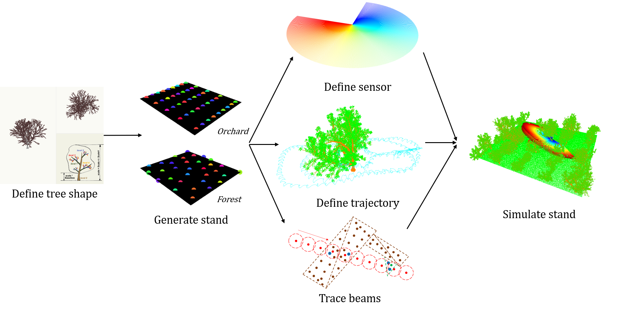
Figure 1: Graphical overview of how SimTreeLS works

2 Method

SimTreeLS is designed to be extensible to a range of situations. In this section, we describe how the system is set up, from defining tree shape and organisation through to simulating the scanning process itself. We then explain the validation experiments with which we demonstrate the suitability and capabilities of SimTreeLS for use as a data generation tool. The core components of SimTreeLS are the open source libraries Comma and Snark (Australian Centre for Field Robotics (2012) [ACFR]). SimTreeLS is available at https://github.com/fwestling/SimTreeLS.

2.1 Simulating scans

2.1.1 Defining trees

To generate tree model objects, we use the Arbaro software made by Diestel [2003] and based on the work of Weber and Penn [1995]. Arbaro provides a number of predefined realistic tree definitions, and allows the user to create new definitions to suit the tree shapes in which they are interested, using the interface shown in Figure 2. The tree definitions are encoded in XML format, which is used as an input for SimTreeLS. We run the Arbaro command line interface using a tree definition to generate an individual tree as a 3d mesh in OBJ format. By providing varying seeds for a random generator, different individuals can be produced using the same definition, and we use the seed of a particular individual tree as its ID for later processing.

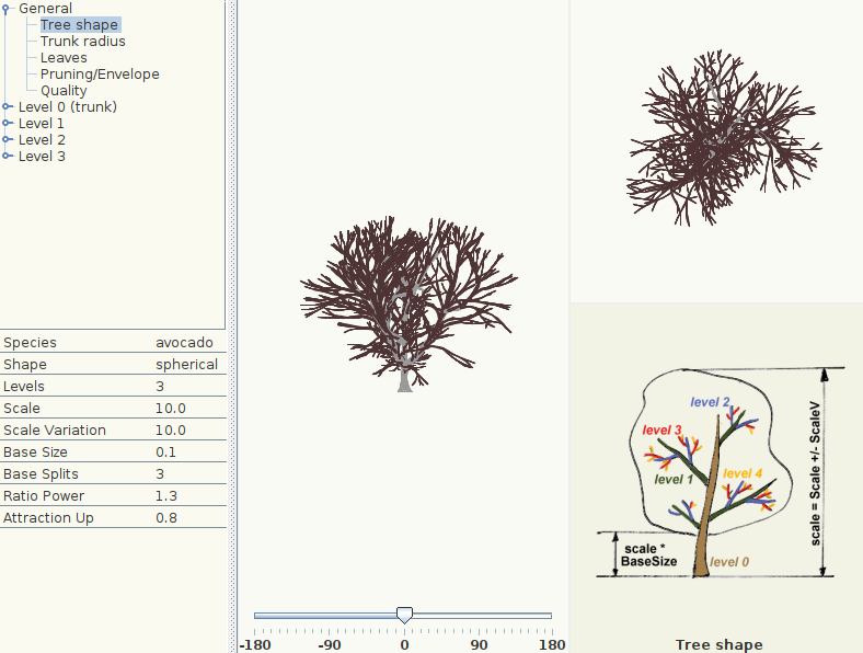
Figure 2: Screenshot of Arbaro tree generation software with a customised tree definition (Diestel [2003])

When generating a dataset, SimTreeLS calculates how many trees are required and generates the necessary OBJ files, then performs mesh sampling to turn the tree meshes into very high density point clouds with no noise. This is required for our sampling method used later in the process; although the mesh file could potentially be used directly, our method (described below) operates on point clouds. The sampling density is chosen to be high enough that the distance between points is smaller than the search radius for a single sensor beam, such that if a beam passes through an element of the mesh it should detect the sampled points at that location.

Simulating the trees like this provides perfectly and completely labelled data, as every point in the point cloud is marked according to which level of branch it represents, from Level 0 (trunk) to Level 3 (leaf).

2.1.2 Organising stands

SimTreeLS is designed primarily for use in agriculture and forestry, where trees are typically processed at large scale rather than individually. Therefore, we included the ability to simulate collections of trees that we call ”stands” in two pre-defined formats, shown in Figure 3. The ”orchard” format organises trees in straight rows, with user-defined values for tree spacing and row spacing. The rows are by default north-aligned, but can easily be rotated to any angles, which has allowed orientation experiments presented by Westling et al. [2020a]. The ”forest” format arranges trees randomly, with a user-defined minimum distance between them.

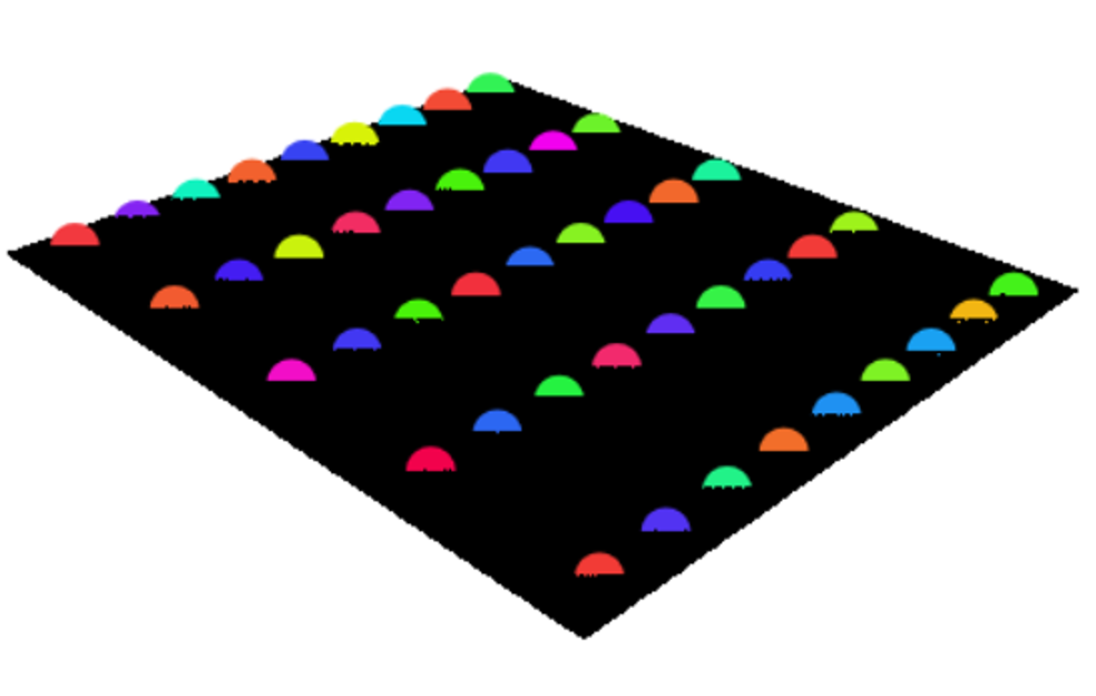
(a) Orchard

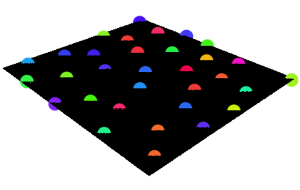
(b) Forest

Figure 3: Different stand layouts for agriculture and forestry. The orchard layout is procedural with row and tree spacing as user-defined parameters, while the forest layout is non-deterministically generated while enforcing a minimum spacing between trees. Each coloured point shown is selected as the trunk location of a simulated tree to be added later. The spacing of the orchard trees is 4m (tree) / 10m (row) for easy of visibility, though for our experiments we use 6m / 10m. The spacing for the forest trees in this example has been set to a minimum of 6m.

2.1.3 Sensors and trajectories

To simulate realistic LiDAR scans, we define a LiDAR sensor shape and a trajectory. The sensor shape is created as a point cloud such that it is not limited to simple planes, but can easily be extended to other definitions like composites (e.g. multi-plane LiDAR) or spherical (e.g. rapidly rotating LiDAR). For any sensor definition, the points should be organised as ”scan lines” which represent the path of the laser at any given time. The distance between points within a scan line is determined by the distance accuracy and angular resolution of the specific sensor being simulated, and each individual scan line is assigned a unique identifier to control occlusion. Figure 4 shows some example LiDAR definitions. This format allows us to use point cloud comparison tools provided by Snark, as well as allowing multi-plane sensors like the Velodyne Puck to be simulated as easily as a 2D sensor, as is shown in the figure. Trajectories are simply defined as a list of points with associated quaternions to define the pose of the LiDAR at each time step. Figure 5 shows an example trajectory based on a scan using a handheld sensor (GeoSLAM Zeb1, Bosse et al. [2012]). This trajectory is a loop around a central tree designed to maximise the information captured on that tree, with little concern for surroundings. This trajectory is useful for studying SimTreeLS due to its complexity and because it was designed to minimise occlusion, but simpler trajectories can also be used.

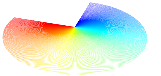
(a) Single-beam LiDAR

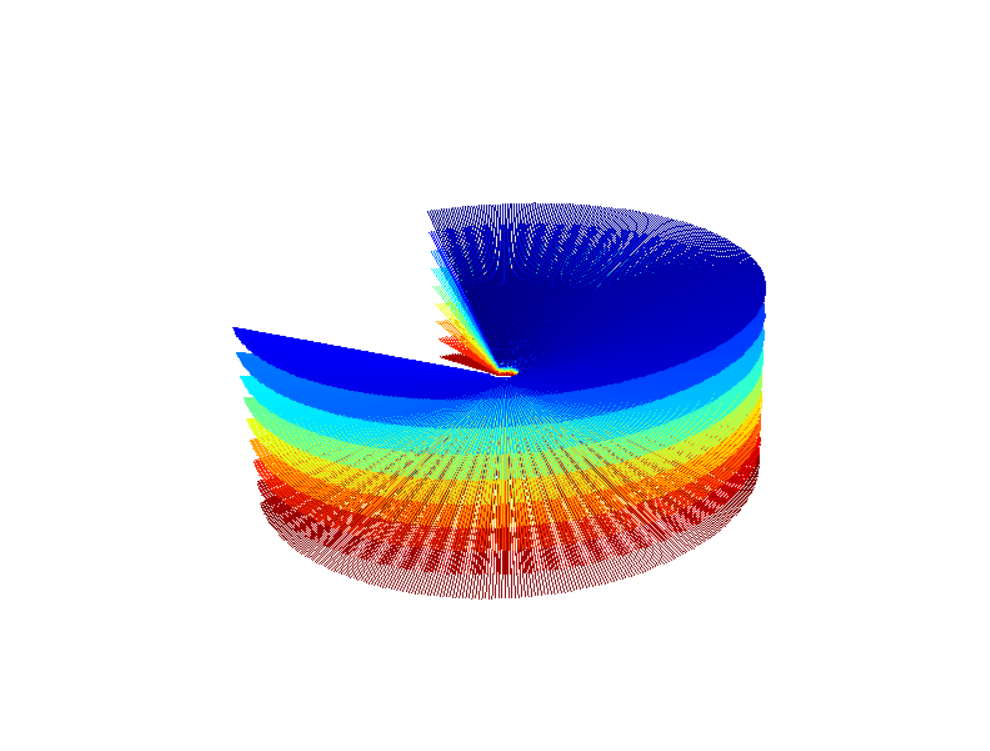
(b) 9-beam LiDAR

Figure 4: Example sensor shape definitions for two different LiDAR sensors. The sensor has been simulated with $270\deg$ range, $0.675\deg$ angular resolution and 15m range, and presented as a single-plane LiDAR as well as a 9-beam LiDAR with a vertical range of $30\deg$. Each beam has a unique identifier related to its angular position, here coloured from blue to red.

Traditional approaches to ray tracing such as that presented by Li et al. [2020] define rays as lines and keep the mesh being scanned as a list of shapes, whereas we represent both the sensor and the mesh as a point cloud. While this leads to larger memory requirements on the data, it enables optimisations and parallelisation using existing point cloud processing tools. In particular, this data formulation allows the use of the Snark library, which is optimised for fast streaming processes on point cloud data. Other commonly used optimisations for point clouds, for instance octrees, could further be applied to improve processing speeds.

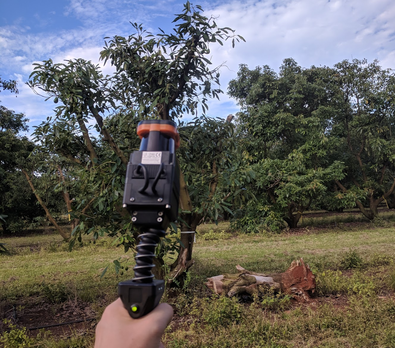
(a) Sensor used to generate trajectory

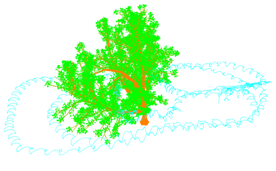
(b) Trajectory in silico

Figure 5: Example sensor trajectory based on the trajectory of a GeoSLAM Zeb1. The trajectory is here overlaid on a virtual tree with trunk located at (0,0,0). The path followed is a double closed-loop trajectory employing a wide circle for context and a close circle for occlusion minimisation. The sensor generates a 3D scan by oscillating the 2D sensor, causing the particular shape seen in the trajectory.

2.1.4 Simulating LiDAR scans

The process of simulating the LiDAR scan is relatively simple, since the stands, trajectory and sensor are defined. The sensor shape is moved to each point in the trajectory in turn, and from each location, the scanning process is performed. A snapshot of the sensor placement process is illustrated for three different trajectories in Figure 6.

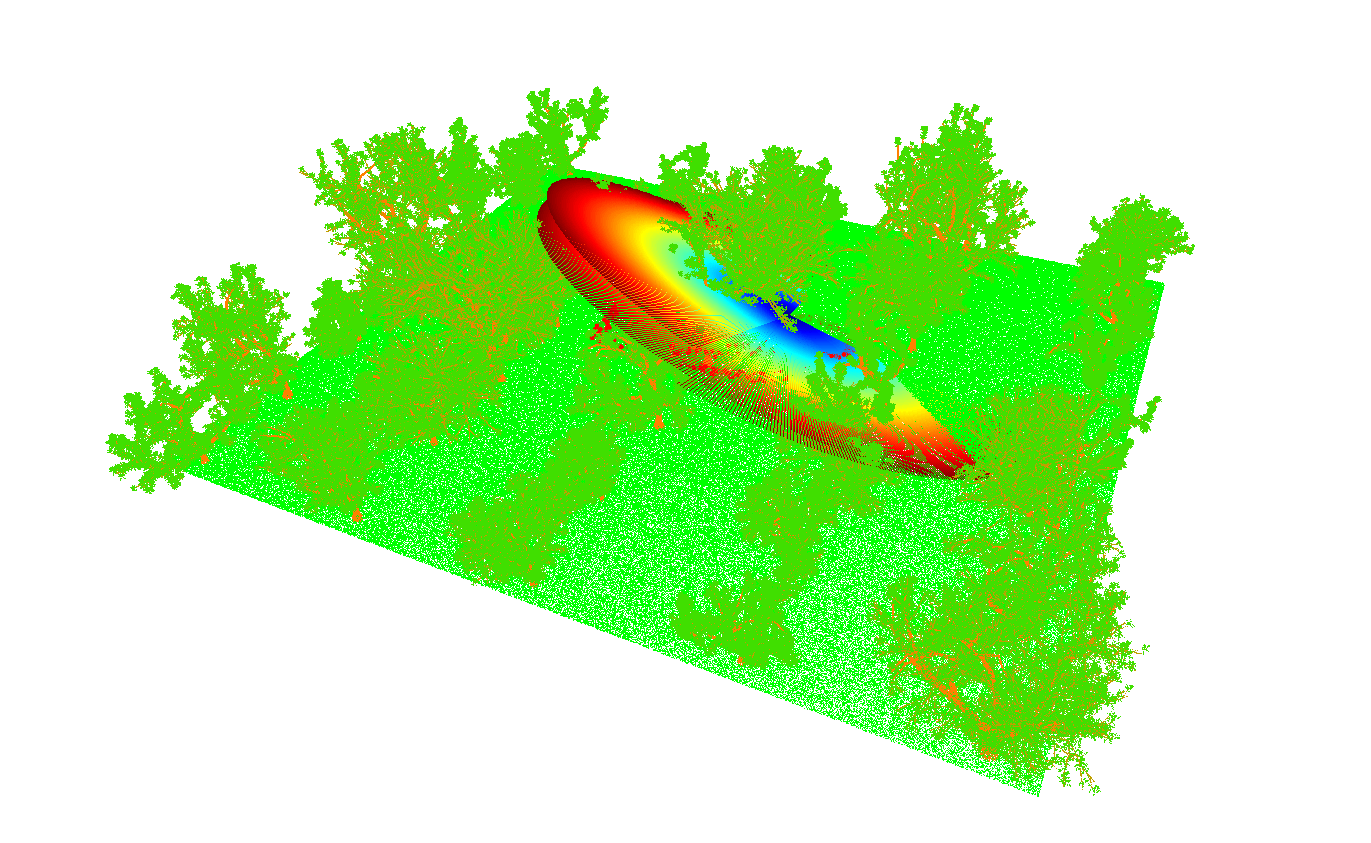
(a) GeoSLAM Zeb1

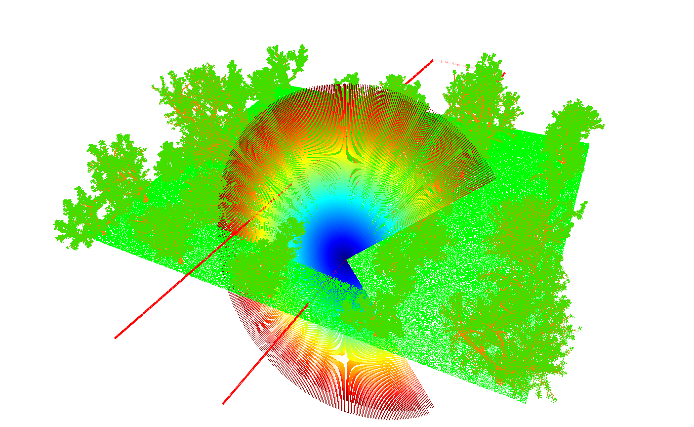
(b) Mobile platform

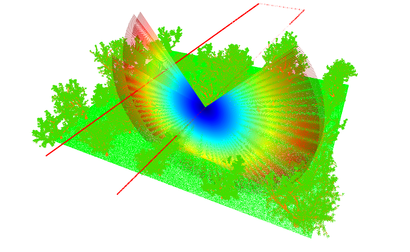
(c) Aerial scan

Figure 6: Snapshot visualisation of scan simulation, with the sensor shape at a point in the trajectory overlaid on a stand of trees (orchard, 6m / 10m spacing). Here we show three different trajectories, simulating handheld, mobile and aerial LiDAR.

At each location, the points of the sensor shape are mapped to their nearest point in the high-density point cloud representing the stand of trees. Each point in the scan plane is only matched to points within a certain radius, selected as the error of the sensor being simulated. Since each scan line has a unique identifier, only match closest to the sensor origin for each scan line is kept, so that occlusion is handled correctly. This process is illustrated in Figure 7. Once a first-return point has been selected, gaussian noise with a user-defined mean is added to the coordinates of that point to simulate the effects of sensor noise and tree movement due to wind.

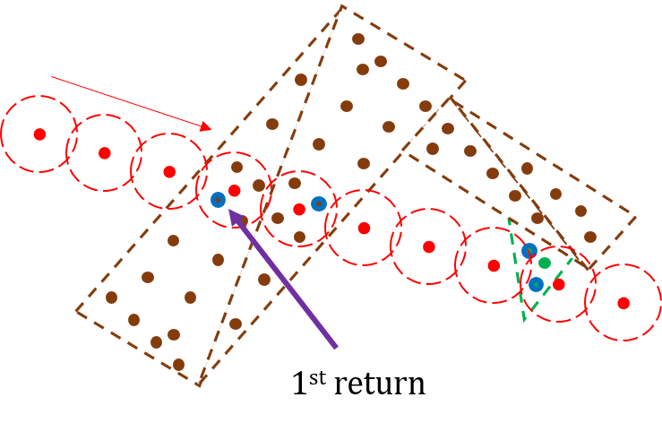
Figure 7: Illustration of scan simulation process for a single scan line in the high density point cloud. Brown and green points represent the tree being scanned. Red points represent the points in the scan line, with a dotted border to signify the search radius. Points circled in blue are identified as candidate points detected by this scan line, and only the first one is returned, such that the green leaf is ”occluded” from this scan line.

2.2 Validation Experiments

Since the input tree objects are generated in silico, there is no option to collect ground truth data using real LiDAR. However, our aim is to validate that the point clouds produced by SimTreeLS are similar in nature to those captured by real LiDAR, so we can compare metrics which are characteristic of LiDAR scans in these environments.

The metric we are demonstrating is the scan density: when scanning with a real LiDAR, the density of the point cloud is non-uniform and dependent on the distance of the object from the sensor, occlusion, and a variety of other influences. We examined the average and deviation of the point cloud density as a function of height and distance from the origin.

To validate our scans, we compared a representative scan of avocado trees using a GeoSLAM Zeb1 handheld LiDAR with point cloud generated by SimTreeLS. We also generated control point clouds by performing mesh sampling without any sensor simulation, at a sampling density which leads the final cloud to have a similar number of points as the simulated clouds. This is the easiest way to turn the high density point cloud into simulated point cloud data, but does not incorporate any occlusion or sensor range limitations. We aimed to show that SimTreeLS outputs are closer to real LiDAR scan data than those generated by this simpler approach.

Since the intent of these simulations is to generate usable data, we also test the applicability of the results to tree analysis operations. Specifically, we used the graph-based trunk classification and individual segmentation process presented by Westling et al. [2020b] on large quantities of real data as well as virtual data, and performed a two-tailed unpaired T test to see whether the results are conceivably from similar distributions.

2.3 Applications

Simulated tree data has other applications beyond simply replacing real data. In this section, we describe the experiments we performed to illustrate some of these applications.

One such application is the capability of SimTreeLS to simulate a range of scanning contexts, which can be used to estimate the value of a particular sensing modality. Validation experiments described in the previous section were conducted using the ”Zeb1” trajectory, which simulates the trajectory of the handheld LiDAR. Other common trajectories for orchard scanning are terrestrial mobile platforms like the SHRIMP platform presented by Underwood et al. [2016] or scanning by aerial drone-mounted LiDAR such as Almeida et al. [2019]. We simulated scans of different trees scanned by simulated trajectories in these additional contexts to show the difference in density characteristics.

Another application made possible by simulated data is the analysis of occlusion, which is a significant reason that real scans may not show the full context of the scene. To investigate this, we examined the occlusion profile of different scanning contexts as compared to a simply sampled control. We estimated occlusion by mapping the point cloud from the simulated scan back to the original high-quality point cloud to identify occluded matter, within a small search radius.

We also performed the same analyses of density and occlusion using two additional tree definitions to show the flexibility of the system, as well as a forest-style stand, with a random distribution of trees at a minimum tree spacing of 6m. The additional datasets are visualised in Figure 8.

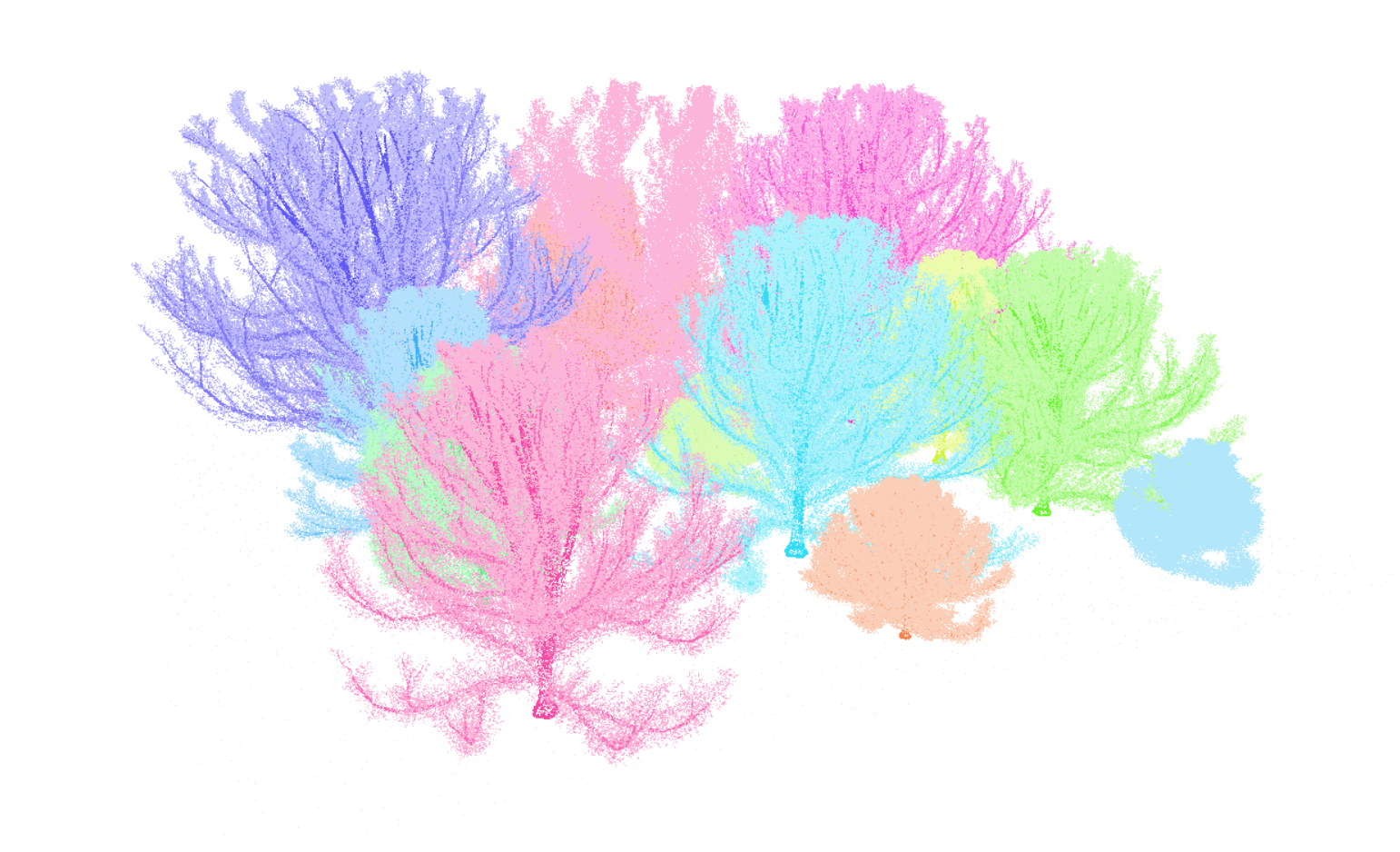
(a) Macadamia orchard

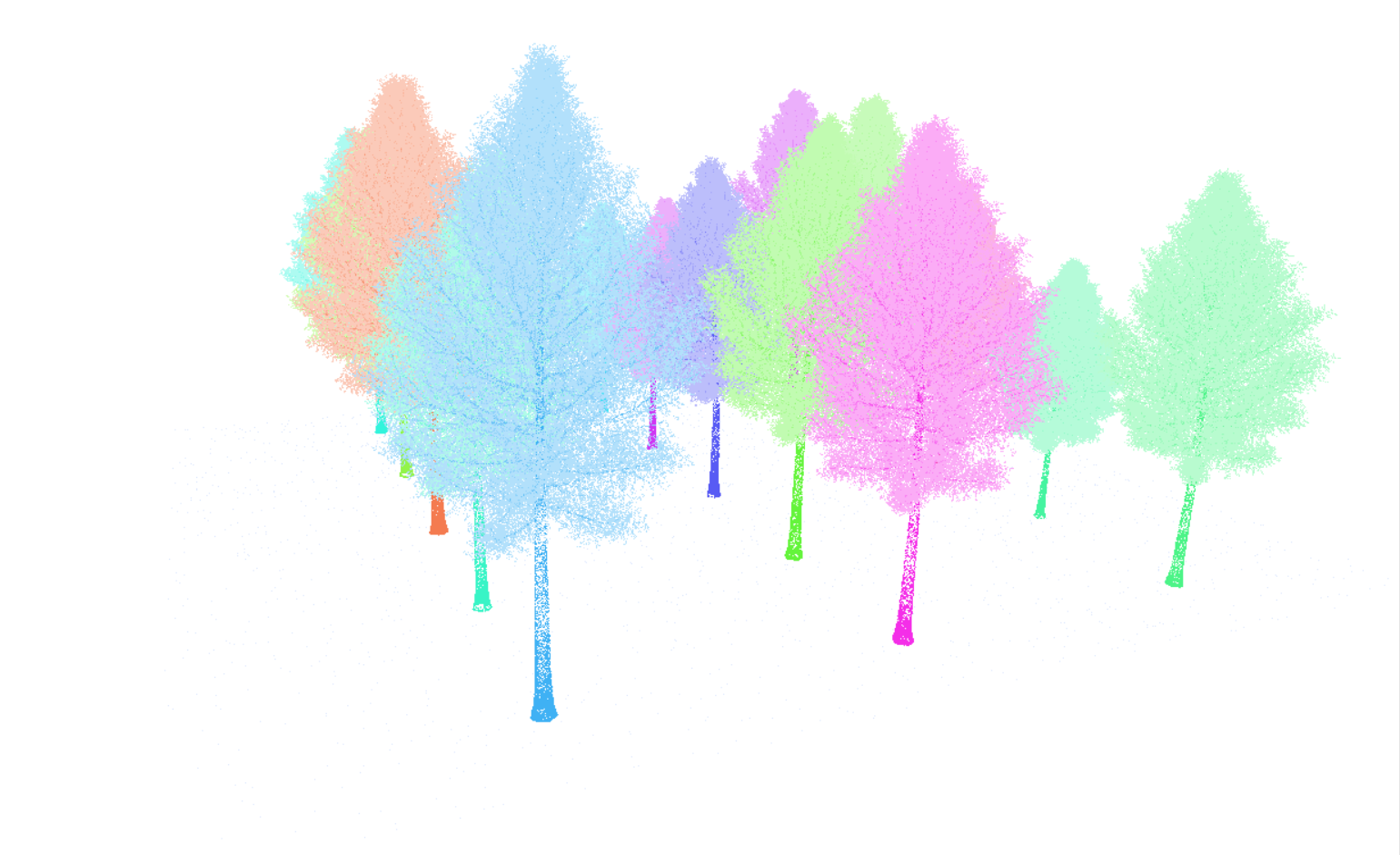
(b) Aspen orchard

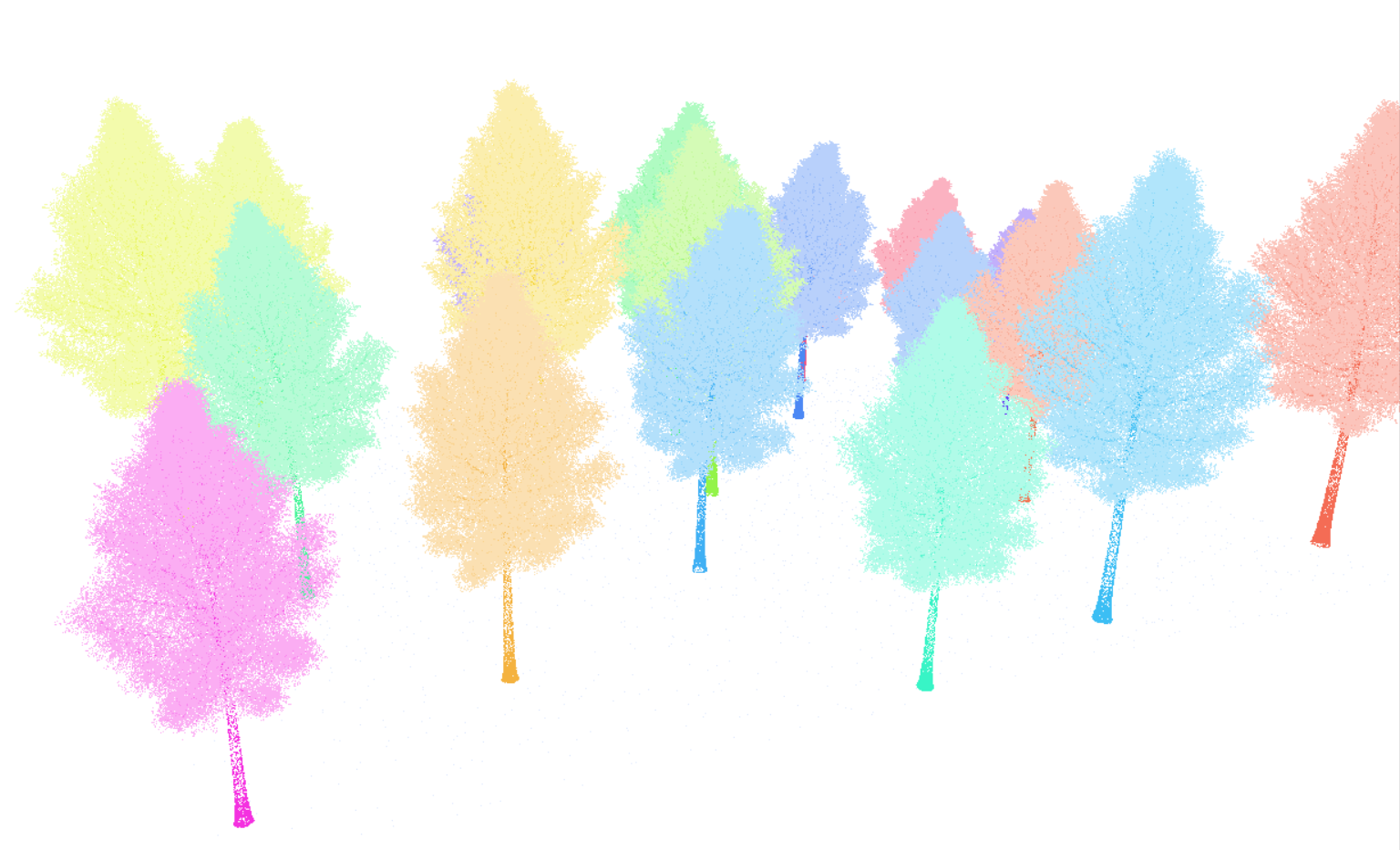
(c) Aspen forest

Figure 8: Additional tree and stand definitions used in application experiments.

3 Results

In this section, we present the results of basic SimTreeLS operation.

3.1 SimTreeLS outputs

We first demonstrate a visual example of the scan simulation outputs. An example of a single simulated tree is shown in Figure 9. A close up of a tree simulated at different levels of noise is also shown in Figure 10. We present an example of a real LiDAR scan using the same sensor we are simulating for comparison.

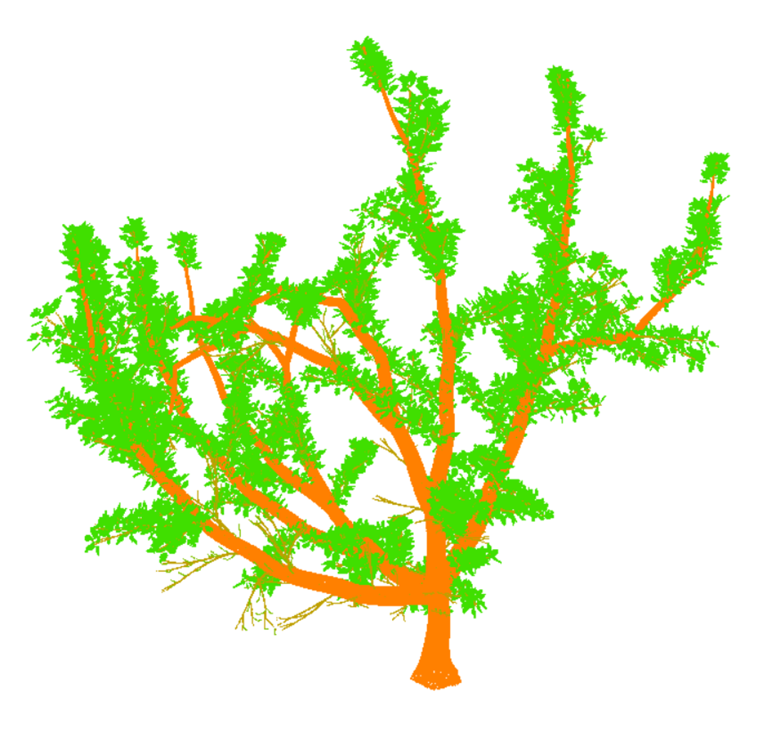
(a) High density point cloud from Arbaro

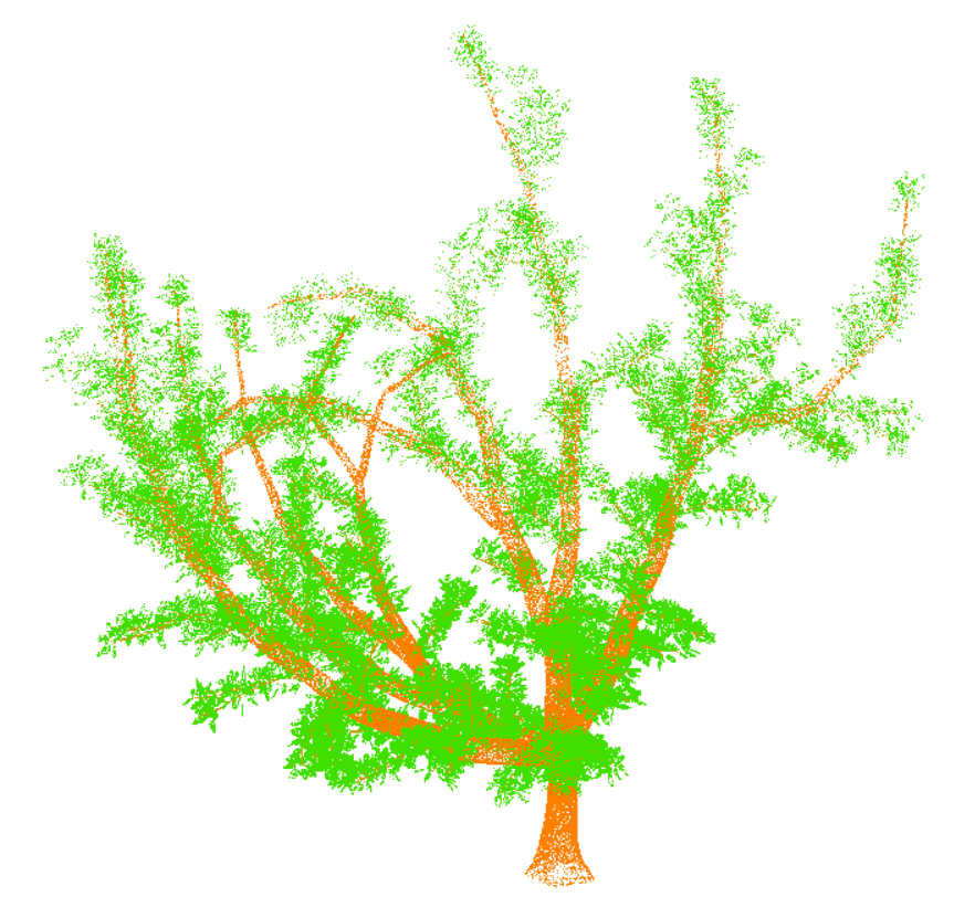
(b) Simulated scan

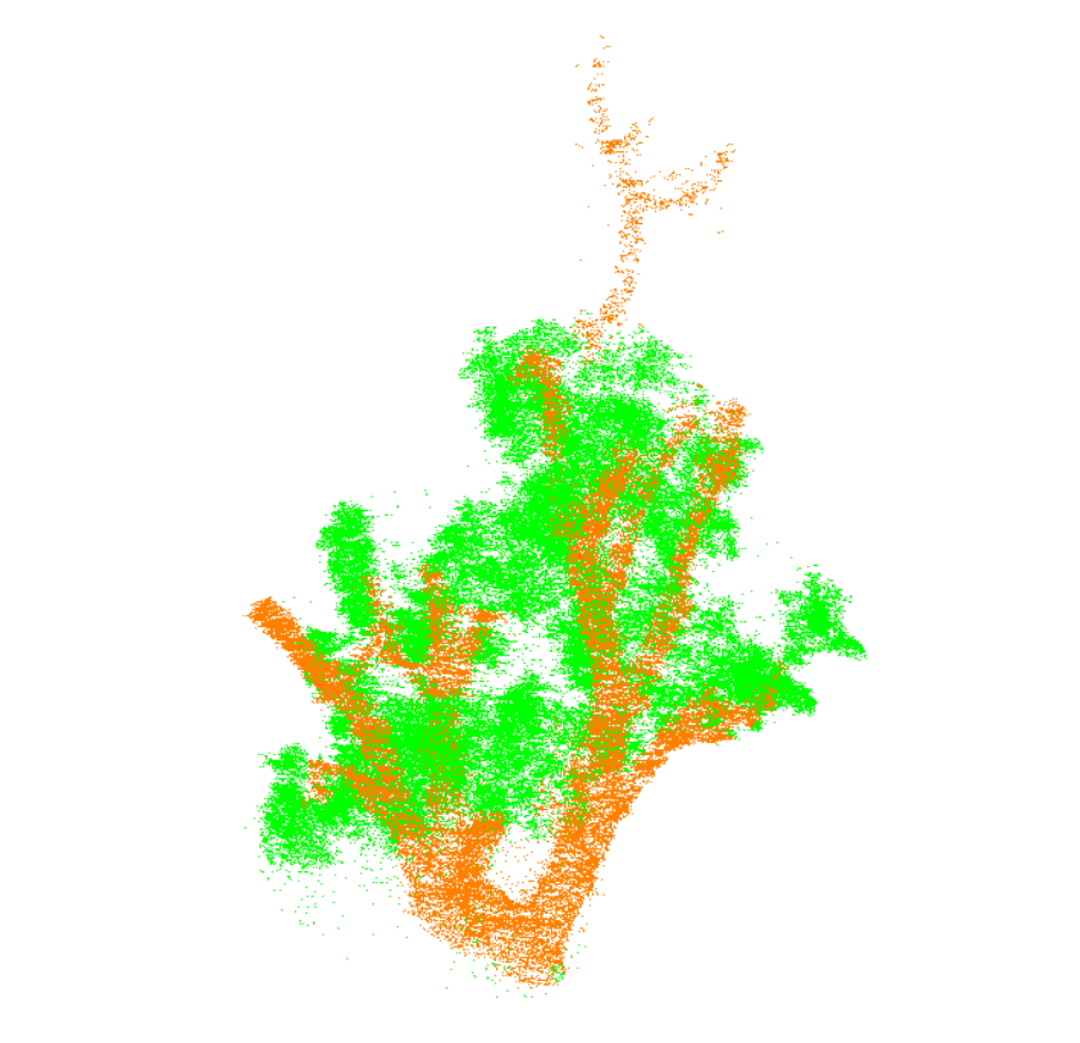
(c) Real scan

Figure 9: Visualisation of a virtual tree before and after LiDAR simulation. The tree shown was simulated at the focus of the Zeb1 trajectory. The points are coloured according to their classification, from orange at Level 0 (trunk) to green at Level 3 (leaf). A real scan of an avocado tree (with manually labelled trunks) is also shown for comparison. Note that these trees are not the same shape originally, as the virtual tree is procedurally generated using a tree definition designed to be similar to avocado trees, rather than a model of the same tree shown in the real scan. The similarities in the different point clouds are primarily seen in the structural characteristics, for instance the changing density of the scan towards the upper canopy.

A visualisation of an entire scan simulated using the Zeb1 trajectory is also shown in Figure 11

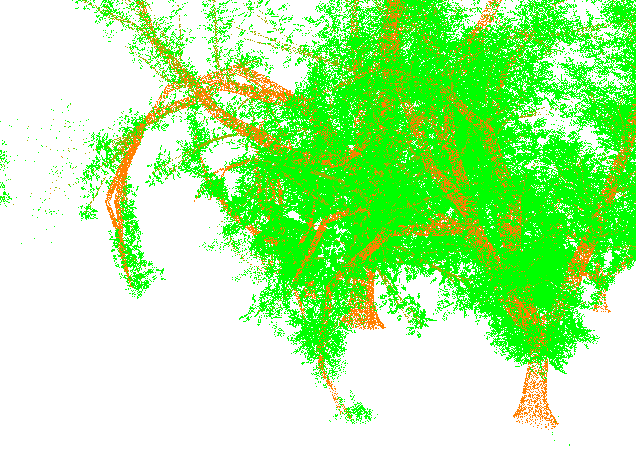
(a) No noise

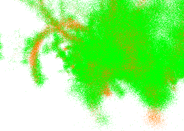
(b) Noise parameter = 0.1m

Figure 10: Effect of simulated noise on outputs. The tree in (a) has been simulated with a Zeb1 trajectory an no added noise, while the more extreme tree in (b) has been simulated with the same trajectory and a noise level of 0.1m. The other simulations used in this paper were simulated at 0.02m.

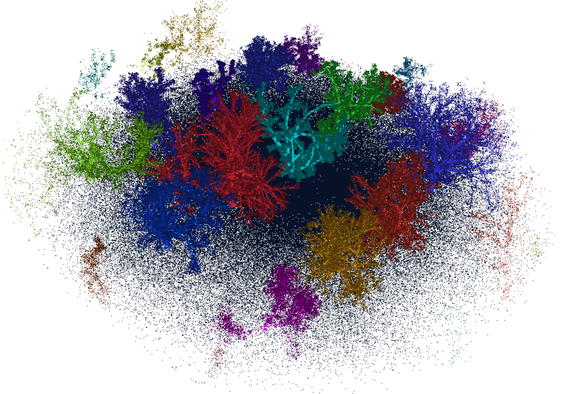
Figure 11: Visualisation of a whole stand of trees in orchard format, simulated using the Zeb1 trajectory. Trees are coloured according to their unique ID, with brighter colours for trunk matter. Viewing in colour is recommended.

3.2 Validation experiments

Here we present results for experiments validating our method using scan density.

Table I presents numerical results for the datasets used in validation. All the trees in this set are either real avocado trees or trees generated using an Arbaro definition designed to replicate avocado trees.

	Real	Control	Simulated
Number of points	5467474	2082868	2047514
% of points occluded	N/A	18.2%	56.3%
Average density $pts/m^{3}$	11518.8	3267.3	6813.1
Stddev density $pts/m^{3}$	27152.3	3155.5	15872.8

TABLE I: Experimental results for validation experiments. All stands shown were simulated using the same sensor definition, modelled after the sensor used to generate the real scan. The simulated cloud here was generated using ”Avocado” style trees, ”Zeb1” trajectory and single-plane sensor shape.

We validate the scan density by plotting the scan density as a function of location and comparing the results for a real Zeb1 scan, a control point cloud generated through random sampling, and a simulated Zeb1 scan. The scan density was considered in two contexts. First, the density was examined as a function of distance from the origin of the point cloud. This was chosen because the Zeb1 trajectory is specifically targeted at the central tree, leaving trees on the periphery less densely scanned as a result. Secondly, the density as a function of height was considered. This was because the scan density is low at the higher ends of the tree due to occlusion and beam scattering during scanning. The plots for these functions, measured across all three point clouds, are shown in Figure 12.

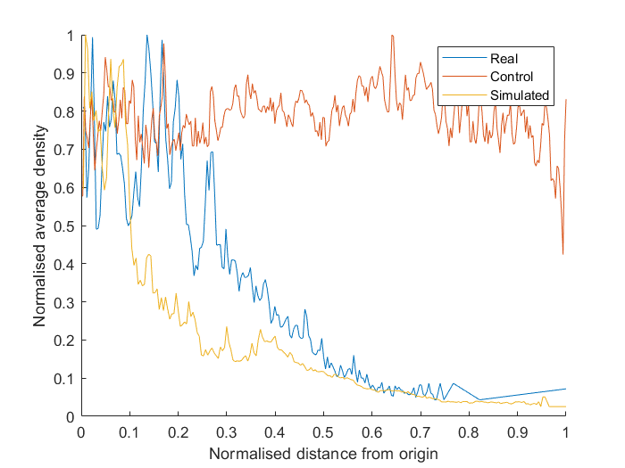
(a) Density against XY distance from the origin

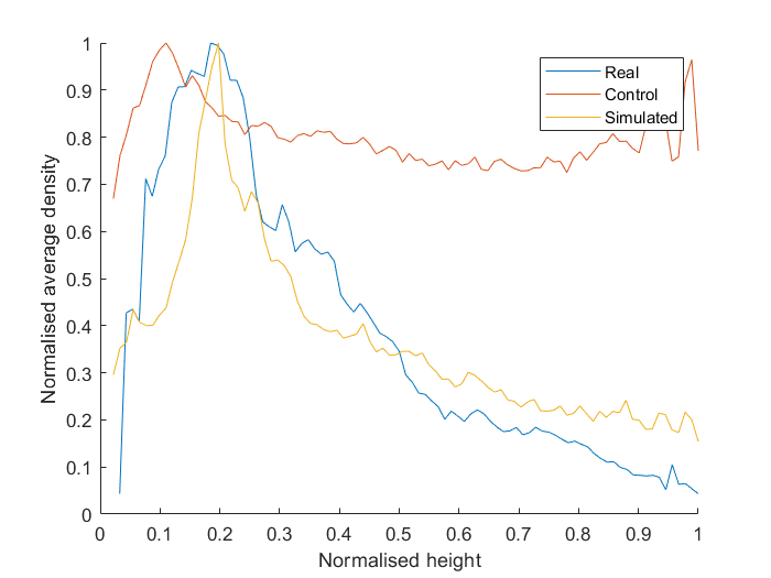
(b) Density against height

Figure 12: Validation results for scan density. Here we present density as a function of XY distance from the origin and the height above the ground. The control was generated using simple mesh sampling such that the number of points was close to the simulated results. Note that the distances and density are normalised due to the difference in shape between the real and simulated trees.

Results from our applicability validation are shown in Table II. The values presented are the mean and variance for the primary metric used to quantify the performance for classification and segmentation, namely F1 score and V-Measure (Rosenberg and Hirschberg [2007]) respectively. An unpaired t-test was also performed between the two datasets to test whether they were statistically similar, and the p value is reported.

	Classification	Segmentation
Real mean	0.4394	0.9047
Real variance	0.0148	0.0082
Virtual mean	0.5123	0.8824
Virtual variance	0.0048	0.001
T-test p value	0.0163	0.0422

TABLE II: Results for trunk classification and individual segmentation for real versus simulated trees (orchard, avocado). Virtual results are over a range of tree spacings from 4m to 8m.

3.3 Applications

For our applications, we process new datasets using alternative tree definitions and stand layouts. A numerical summary of all these experiments, detailing the occlusion and density of the results, is provided in Table III.

	Avocado orchard
	Control	Zeb1	Mobile	Drone
Number of points	2082868	2047514	2110775	563379
% of points occluded	18.17%	56.28%	50.68%	64.26%
Average density (pts/m^3)	3267.3	6813.1	6433.6	2564.7
Stddev density (pts/m^3)	3155.5	15872.8	13856.3	2835.9
	Aspen orchard
Number of points	2713915	1482655	1447140	1620340
% of points occluded	14.42%	52.42%	45.58%	38.66%
Average density (pts/m^3)	3627.5	3466.3	2957.6	3011.2
Stddev density (pts/m^3)	4021.1	5600.7	3765.3	3111.9
	Aspen Forest
Number of points	3548336	1428058	1621777	1925538
% of points occluded	13.86%	55.74%	53.71%	48.69%
Average density (pts/m^3)	3915.2	3356.1	3365.1	3486.7
Stddev density (pts/m^3)	4520.1	6806.7	5677.4	4641.1
	Macadamia orchard
Number of points	3512419	4973296	3311894	1883430
% of points occluded	18.15%	44.07%	44.57%	48.04%
Average density (pts/m^3)	3686.0	7392.2	4910.2	2987.5
Stddev density (pts/m^3)	4844.0	43754.8	10491.7	5525.6

TABLE III: Experimental results for applications. All stands shown were simulated using the same sensor definition, modelled after the sensor used to generate the real scan. These are all virtually generated trees.

For a visual example of the results, an occlusion map of each trajectory is presented in Figure 13, along with the aerial trajectory for the forest stand. Points in red are considered occluded while points in green are considered scanned. We also include a 9-beam LiDAR for comparison with the Mobile trajectory, demonstrating the difference in occlusion using a LiDAR with more data in the same trajectory.

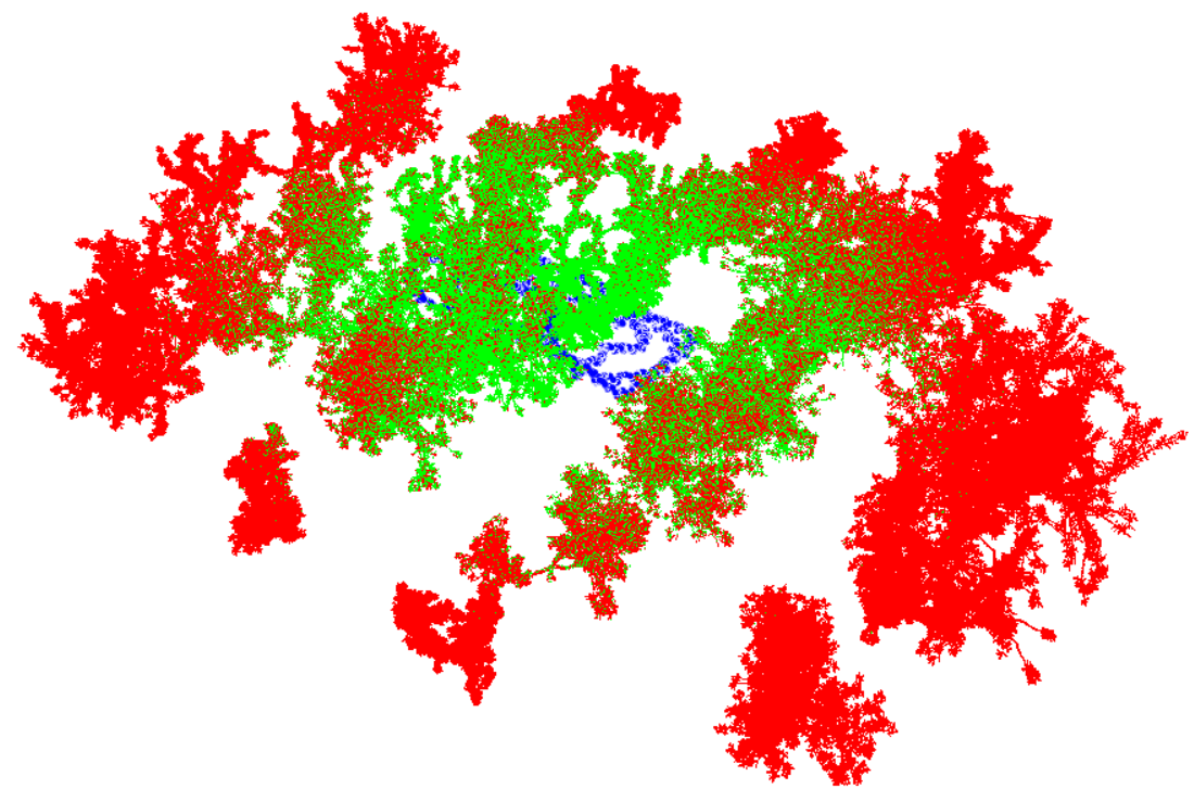
(a) Zeb1

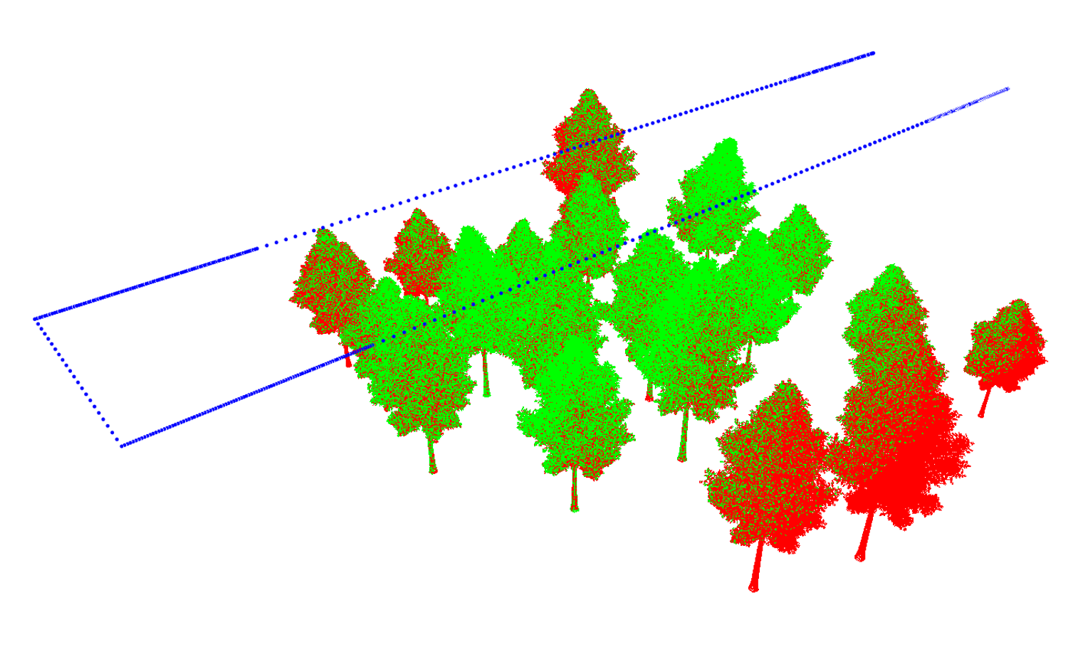
(b) Forest (drone)

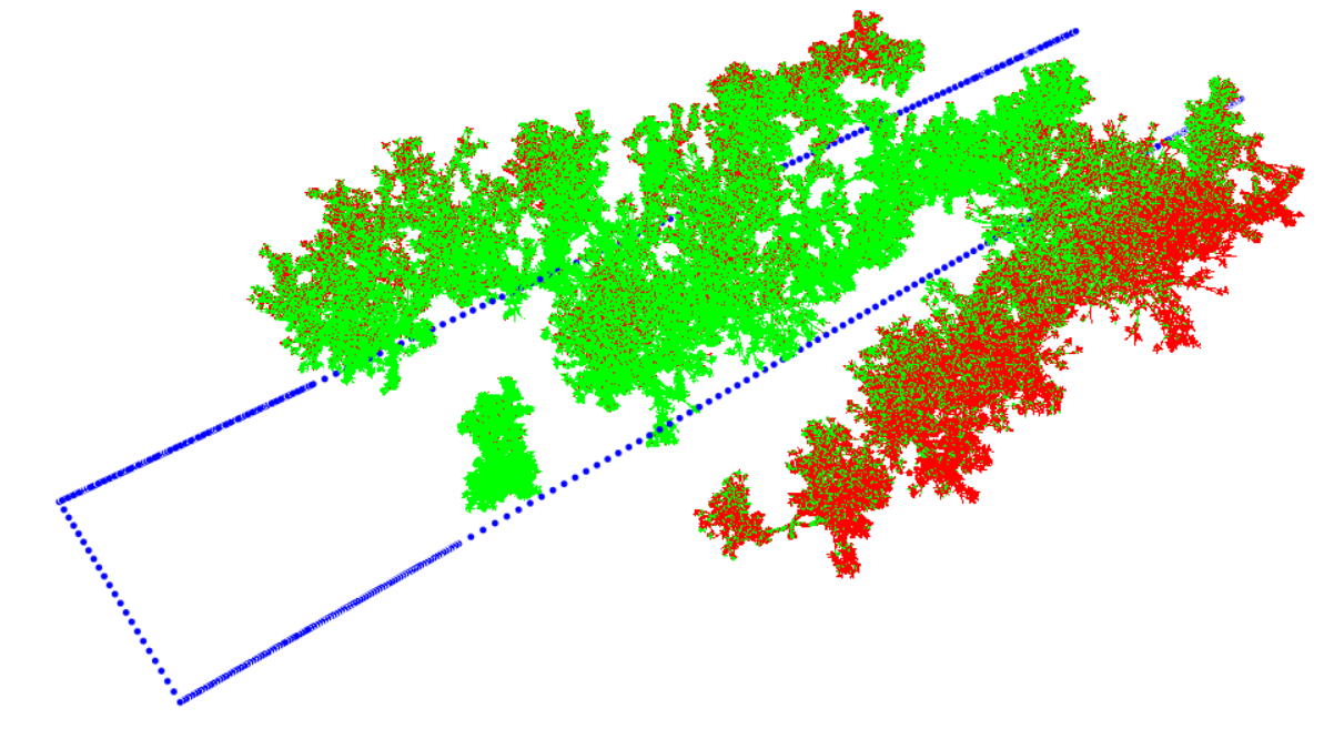
(c) Mobile

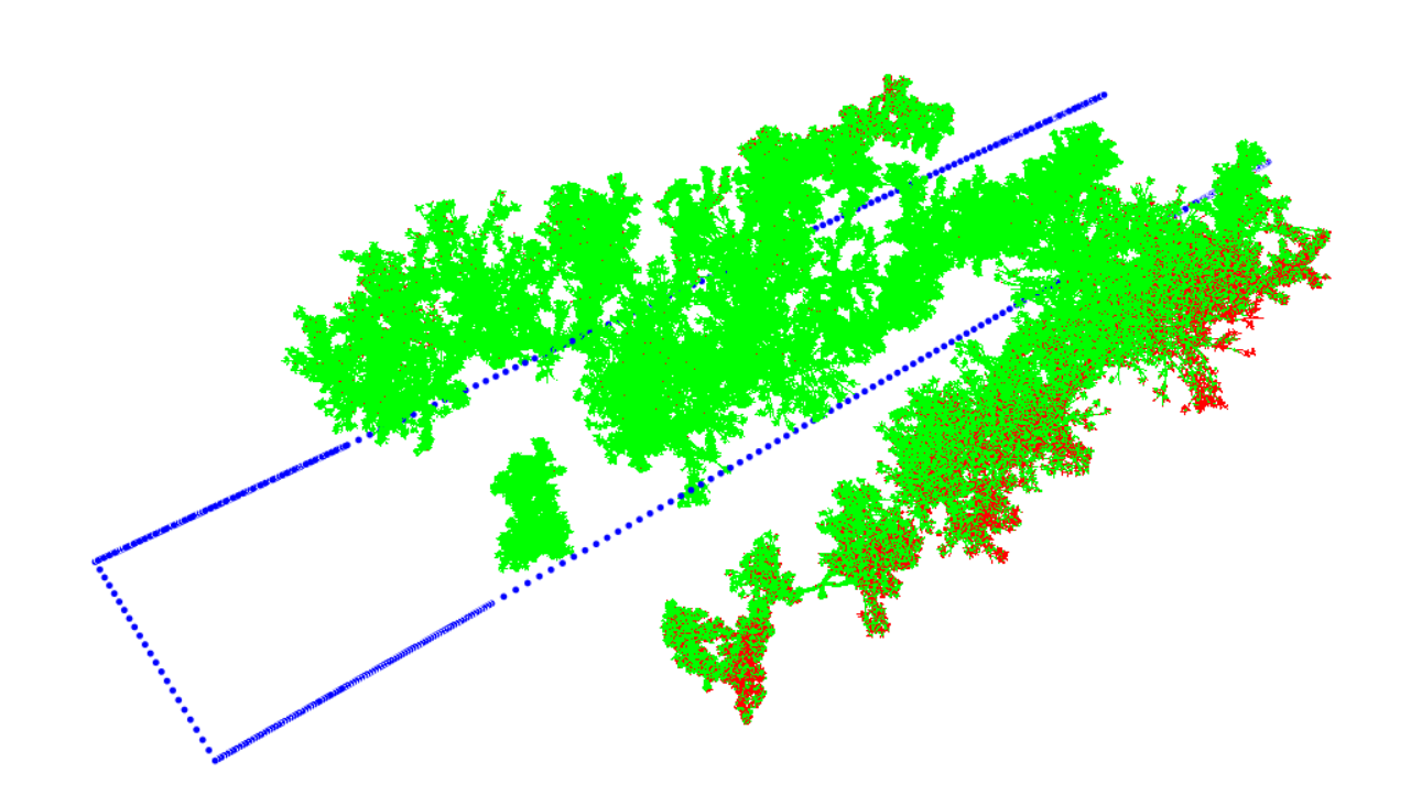
(d) Mobile (9-beam LiDAR)

Figure 13: Examples of occlusion maps for different trajectory types as compared to the control set. Points from the original stand which are visible in the simulated scan are in green, the others are in red. The trajectories used to generate the scans are shown in blue where applicable.

4 Discussion

In this section we discuss the results presented in the previous section, and suggest areas for future work. Generally, the outputs of SimTreeLS present point clouds which are similar in structure and form to those generated by real LiDAR, and are easy to customise for a particular application.

The differences in real versus virtual trees can generally be characterised as a difference tree shapes and noise characteristics. One of the main causes of discrepancies is our current inability to simulate tree motion. Regardless of the method used for LiDAR scanning, the motion of the tree due to wind will introduce potentially significant noise, depending on the strength of the wind. This effect can be seen in Figure 9, where branches present with greater thickness than the virtual results, and leaves are shown as less distinct.

4.1 Validation

The validation results show that the outputs are reasonable approximations of reality. Given that the simulated trees were not identical to the real ones (instead just a rough facsimile), we did not expect perfect replication, but rather a strong correlation. The number of points shown in Table I suggest that the trees generated by Arbaro are potentially smaller than the real ones, leading to a smaller final point cloud. However, we also see the relative difference between average and standard deviation of density being similar, suggesting a similar pattern of scanning, as opposed to the control. Figure 12 reinforces this point further, with both graphs for control being clearly different to the real ones, but the simulated graphs sharing characteristics with the real data. This implies that the simulated scans generate data which is structurally similar to that generated by real sensors in the case of the Zeb1 trajectory.

The results of classification and segmentation of real and virtual data presented in Table II further illustrate how SimTreeLS generates data with similar structure to real LiDAR scans. The results of the t-test imply that the two datasets are distinct, with a p value of 0.04 for segmentation and 0.01 for classification. The disparity between the datasets could be explained by errors in manual labelling due to indistinct areas and tree overlap for the real data, or because the virtual trees are merely approximations of the avocado tree structure.

4.2 Applications

The results for our applications illustrate the flexibility of SimTreeLS, and show that alternate trajectories and tree definitions also produce realistic results. The additional stands tested, shown in Figure 6, demonstrate particular characteristics not shown by the avocado orchard stand used in the validation experiments. The ”macadamia” tree definition is much wider than the other trees, so using the same stand definition leads to a much denser orchard, which is not unusual in commercial practices. The ”aspen” trees on the other hand have their foliage high up in the canopy, which is above the focus of the Zeb1 trajectory, and significantly denser than the other trees, which should show a high occlusion. The forest stand is interesting since the trajectories were designed to optimise scanning of the orchard definition, with the Zeb1 trajectory specifically focused on the central tree. This suggests the ability for SimTreeLS to be used in evaluation and optimisation of trajectories for particular contexts. For instance, given a known sensor in a forestry setting and a set of constraints on potential trajectories, one could be found which maximised scan density or minimised occlusions.

The sensor definition can also make a big difference, for instance the mobile trajectory shown in Figure  13 demonstrates the occlusion with a 9-beam sensor is significantly lower than one with a single beam. It could be anticipated that more data should be detected with the larger sensor, but the additional angles provided significantly more

The results presented in Table III support the intuitive implications of these different stands, as well as suggesting useful insights. For the macadamia trees, the high density of the foliage leads to a large standard deviation across the different trajectories, since the outside of the tree is well scanned and the inside is significantly more occluded. The aspen trees are the only examples where the aerial trajectory has the largest number of points in the output as well as the smallest occlusion. The standard deviation also suggests a very even distribution of scanned points, whereas the Zeb1 and Mobile trajectories miss a lot of the detail in the trees. This is further exasperated in the forest layout, where the mobile trajectory in particular (which only catches the foliage in the edges of the scanner) misses significant amounts of the trees since it does not drive along the rows of trees here.

4.3 Future work

SimTreeLS shows promising results in procedural dataset generation, which has the potential to be helpful in deep learning applications using transfer learning. Future work should include validating this proposal so as to make simulated data more appealing for applications where data capture or manual labelling is difficult prohibitive.

The system could also easily be extended to include items beyond trees. Significant amounts of LiDAR research is developed on sampled meshes, similar to the ”control” used in our experiments, but SimTreeLS could use any sensor definition and trajectory to scan arbitrary meshes. For example, there are applications in the construction industry using LiDAR, and there is often a digital model of the design which could be scanned in this way.

With regards to the system itself, many modern LiDAR sensors are able to capture colour or intensity information, as well as multiple returns for each beam. These features would be a simple inclusion in the pipeline used to generate results.

Other potentially exciting extensions of SimTreeLS include the option to suggest an optimal trajectory given a stand and sensor definition. This may be able to inform users as to which approach to take given a particular context, and could be used to minimise time required for fieldwork.

5 Conclusion

We presented a system, SimTreeLS, for generating simulated LiDAR scans of procedurally generated trees in agricultural and forestry contexts. Validation experiments have shown that the generated data is similar in nature to real LiDAR scans, and several capabilities have been explored and visualised.

Acknowledgements

This work is supported by the Australian Centre for Field Robotics (ACFR) at The University of Sydney. For more information about robots and systems for agriculture at the ACFR, please visit http://sydney.edu.au/acfr/agriculture.

References

- Almeida et al. [2019] D. Almeida, E. N. Broadbent, A. M. A. Zambrano, B. E. Wilkinson, M. E. Ferreira, R. Chazdon, P. Meli, E. Gorgens, C. A. Silva, S. C. Stark, et al. Monitoring the structure of forest restoration plantations with a drone-lidar system. International Journal of Applied Earth Observation and Geoinformation, 79:192–198, 2019.
- Apolo-Apolo et al. [2020] O. E. Apolo-Apolo, M. Pérez-Ruiz, J. Martínez-Guanter, and J. Valente. A cloud-based environment for generating yield estimation maps from apple orchards using uav imagery and a deep learning technique. Frontiers in plant science, 11:1086, 2020.
- Arikapudi et al. [2015] R. Arikapudi, S. Vougioukas, and T. Saracoglu. Orchard tree digitization for structural-geometrical modeling. In Precision agriculture’15, pages 161–168. Wageningen Academic Publishers, 2015.
- Australian Centre for Field Robotics (2012) [ACFR] Australian Centre for Field Robotics (ACFR). Comma and snark: generic c++ libraries and utilities for robotics. https://github.com/acfr/, 2012. Accessed: 2017-02-18.
- Bargoti et al. [2015] S. Bargoti, J. P. Underwood, J. I. Nieto, and S. Sukkarieh. A pipeline for trunk detection in trellis structured apple orchards. Journal of field robotics, 32(8):1075–1094, 2015.
- Bauwens et al. [2016] S. Bauwens, H. Bartholomeus, K. Calders, and P. Lejeune. Forest inventory with terrestrial lidar: A comparison of static and hand-held mobile laser scanning. Forests, 7(6):127, 2016.
- Béland et al. [2011] M. Béland, J.-L. Widlowski, R. A. Fournier, J.-F. Côté, and M. M. Verstraete. Estimating leaf area distribution in savanna trees from terrestrial lidar measurements. Agricultural and Forest Meteorology, 151(9):1252–1266, 2011.
- Béland et al. [2014] M. Béland, J.-L. Widlowski, and R. A. Fournier. A model for deriving voxel-level tree leaf area density estimates from ground-based lidar. Environmental Modelling & Software, 51:184–189, 2014.
- Bosse et al. [2012] M. Bosse, R. Zlot, and P. Flick. Zebedee: Design of a spring-mounted 3-d range sensor with application to mobile mapping. IEEE Transactions on Robotics, 28(5):1104–1119, 2012.
- Cao et al. [2019] L. Cao, H. Liu, X. Fu, Z. Zhang, X. Shen, and H. Ruan. Comparison of uav lidar and digital aerial photogrammetry point clouds for estimating forest structural attributes in subtropical planted forests. Forests, 10(2):145, 2019.
- Colaço et al. [2019] A. F. Colaço, J. P. Molin, J. R. Rosell-Polo, et al. Spatial variability in commercial orange groves. part 2: relating canopy geometry to soil attributes and historical yield. Precision Agriculture, 20(4):805–822, 2019.
- Côté et al. [2009] J. F. Côté, J. L. Widlowski, R. A. Fournier, and M. M. Verstraete. The structural and radiative consistency of three-dimensional tree reconstructions from terrestrial lidar. Remote Sensing of Environment, 113(5):1067–1081, 2009. ISSN 00344257. doi: 10.1016/j.rse.2009.01.017. URL http://dx.doi.org/10.1016/j.rse.2009.01.017.
- Da Silva et al. [2014] D. Da Silva, L. Han, and E. Costes. Light interception efficiency of apple trees: a multiscale computational study based on mapplet. Ecological Modelling, 290:45–53, 2014.
- Diestel [2003] W. Diestel. Arbaro—tree generation for povray, 2003.
- Gené-Mola et al. [2019] J. Gené-Mola, E. Gregorio, J. Guevara, F. Auat, R. Sanz-Cortiella, A. Escolà, J. Llorens, J.-R. Morros, J. Ruiz-Hidalgo, V. Vilaplana, et al. Fruit detection in an apple orchard using a mobile terrestrial laser scanner. Biosystems engineering, 187:171–184, 2019.
- Goodin et al. [2019] C. Goodin, S. Sharma, M. Doude, D. Carruth, L. Dabbiru, and C. Hudson. Training of neural networks with automated labeling of simulated sensor data. Technical report, SAE Technical Paper, 2019.
- Guo et al. [2019] Y. Guo, H. Wang, Q. Hu, H. Liu, L. Liu, and M. Bennamoun. Deep learning for 3d point clouds: A survey. arXiv preprint arXiv:1912.12033, 2019.
- Kato et al. [2009] A. Kato, L. M. Moskal, P. Schiess, M. E. Swanson, D. Calhoun, and W. Stuetzle. Capturing tree crown formation through implicit surface reconstruction using airborne lidar data. Remote Sensing of Environment, 113(6):1148–1162, 2009. ISSN 00344257. doi: 10.1016/j.rse.2009.02.010. URL http://dx.doi.org/10.1016/j.rse.2009.02.010.
- Kumar et al. [2019] B. Kumar, B. Lohani, and G. Pandey. Development of deep learning architecture for automatic classification of outdoor mobile lidar data. International Journal of Remote Sensing, 40(9):3543–3554, 2019.
- Lalonde et al. [2006] J. F. Lalonde, N. Vandapel, D. F. Huber, and M. Hebert. Natural terrain classification using three-dimensional ladar data for ground robot mobility. Journal of Field Robotics, 23(10):839–861, 2006. ISSN 15564959. doi: 10.1002/rob.20134.
- LaRue et al. [2020] E. A. LaRue, F. W. Wagner, S. Fei, J. W. Atkins, R. T. Fahey, C. M. Gough, and B. S. Hardiman. Compatibility of aerial and terrestrial lidar for quantifying forest structural diversity. Remote Sensing, 12(9):1407, 2020.
- Li et al. [2020] Y. Li, P. Wang, J. Sun, and X. Gan. Simulation of tree point cloud based on the ray-tracing algorithm and three-dimensional tree model. Biosystems Engineering, 200:259–271, 2020.
- Liang et al. [2016] X. Liang, V. Kankare, J. Hyyppä, Y. Wang, A. Kukko, H. Haggrén, X. Yu, H. Kaartinen, A. Jaakkola, F. Guan, et al. Terrestrial laser scanning in forest inventories. ISPRS Journal of Photogrammetry and Remote Sensing, 115:63–77, 2016.
- Liu et al. [2019] Y. Liu, B. Fan, G. Meng, J. Lu, S. Xiang, and C. Pan. Densepoint: Learning densely contextual representation for efficient point cloud processing. In Proceedings of the IEEE International Conference on Computer Vision, pages 5239–5248, 2019.
- Ma et al. [2016a] L. Ma, G. Zheng, J. U. Eitel, T. S. Magney, and L. M. Moskal. Determining woody-to-total area ratio using terrestrial laser scanning (TLS). Agricultural and Forest Meteorology, 228-229:217–228, 2016a. ISSN 01681923. doi: 10.1016/j.agrformet.2016.06.021. URL http://dx.doi.org/10.1016/j.agrformet.2016.06.021.
- Ma et al. [2016b] L. Ma, G. Zheng, J. U. Eitel, L. M. Moskal, W. He, and H. Huang. Improved Salient Feature-Based Approach for Automatically Separating Photosynthetic and Nonphotosynthetic Components Within Terrestrial Lidar Point Cloud Data of Forest Canopies. IEEE Transactions on Geoscience and Remote Sensing, 54(2):679–696, 2016b. ISSN 01962892. doi: 10.1109/TGRS.2015.2459716.
- Majeed et al. [2020] Y. Majeed, J. Zhang, X. Zhang, L. Fu, M. Karkee, Q. Zhang, and M. D. Whiting. Deep learning based segmentation for automated training of apple trees on trellis wires. Computers and Electronics in Agriculture, 170:105277, 2020.
- Mendez et al. [2012] V. Mendez, H. Catalan, J. R. Rosell, J. Arnó, R. Sanz, and A. Tarquis. Simlidar–simulation of lidar performance in artificially simulated orchards. Biosystems engineering, 111(1):72–82, 2012.
- Nezafat et al. [2019] R. V. Nezafat, O. Sahin, and M. Cetin. Transfer learning using deep neural networks for classification of truck body types based on side-fire lidar data. Journal of Big Data Analytics in Transportation, 1(1):71–82, 2019.
- Pfeiffer et al. [2018] S. A. Pfeiffer, J. Guevara, F. A. Cheein, and R. Sanz. Mechatronic terrestrial lidar for canopy porosity and crown surface estimation. Computers and Electronics in Agriculture, 146:104–113, 2018.
- Qi et al. [2017] C. R. Qi, H. Su, K. Mo, and L. J. Guibas. Pointnet: Deep learning on point sets for 3d classification and segmentation. In Proceedings of the IEEE conference on computer vision and pattern recognition, pages 652–660, 2017.
- Reiser et al. [2018] D. Reiser, M. Vázquez-Arellano, D. S. Paraforos, M. Garrido-Izard, and H. W. Griepentrog. Iterative individual plant clustering in maize with assembled 2d lidar data. Computers in Industry, 99:42–52, 2018.
- Rosell and Sanz [2012] J. R. Rosell and R. Sanz. A review of methods and applications of the geometric characterization of tree crops in agricultural activities. Computers and Electronics in Agriculture, 81:124–141, 2012.
- Rosenberg and Hirschberg [2007] A. Rosenberg and J. Hirschberg. V-measure: A conditional entropy-based external cluster evaluation measure. In Proceedings of the 2007 joint conference on empirical methods in natural language processing and computational natural language learning (EMNLP-CoNLL), pages 410–420, 2007.
- Sanz et al. [2018] R. Sanz, J. Llorens, A. Escolà, J. Arnó, S. Planas, C. Roman, and J. R. Rosell-Polo. Lidar and non-lidar-based canopy parameters to estimate the leaf area in fruit trees and vineyard. Agricultural and Forest Meteorology, 260:229–239, 2018.
- Su et al. [2015] H. Su, S. Maji, E. Kalogerakis, and E. Learned-Miller. Multi-view convolutional neural networks for 3d shape recognition. In Proceedings of the IEEE international conference on computer vision, pages 945–953, 2015.
- Su et al. [2019] Z. Su, S. Li, H. Liu, and Y. Liu. Extracting wood point cloud of individual trees based on geometric features. IEEE Geoscience and Remote Sensing Letters, 16(8):1294–1298, 2019.
- Tang et al. [2015] L. Tang, C. Hou, H. Huang, C. Chen, J. Zou, and D. Lin. Light interception efficiency analysis based on three-dimensional peach canopy models. Ecological Informatics, 30:60–67, 2015.
- Tang et al. [2019] L. Tang, D. Yin, and C. Chen. Optimal design of plant canopy based on light interception: A case study with loquat. Frontiers in Plant Science, 10:364, 2019.
- Tao et al. [2015] S. Tao, Q. Guo, S. Xu, Y. Su, Y. Li, and F. Wu. A geometric method for wood-leaf separation using terrestrial and simulated lidar data. Photogrammetric Engineering & Remote Sensing, 81(10):767–776, 2015.
- Underwood et al. [2016] J. P. Underwood, C. Hung, B. Whelan, and S. Sukkarieh. Mapping almond orchard canopy volume, flowers, fruit and yield using lidar and vision sensors. Computers and Electronics in Agriculture, 130:83–96, 2016.
- Van der Zande et al. [2011] D. Van der Zande, J. Stuckens, W. W. Verstraeten, S. Mereu, B. Muys, and P. Coppin. 3D modeling of light interception in heterogeneous forest canopies using ground-based LiDAR data. International Journal of Applied Earth Observation and Geoinformation, 13(5):792–800, 2011. ISSN 15698432. doi: 10.1016/j.jag.2011.05.005. URL http://dx.doi.org/10.1016/j.jag.2011.05.005.
- Vicari et al. [2019] M. B. Vicari, M. Disney, P. Wilkes, A. Burt, K. Calders, and W. Woodgate. Leaf and wood classification framework for terrestrial lidar point clouds. Methods in Ecology and Evolution, 10(5):680–694, 2019.
- Wang et al. [2019] F. Wang, Y. Zhuang, H. Gu, and H. Hu. Automatic generation of synthetic lidar point clouds for 3-d data analysis. IEEE Transactions on Instrumentation and Measurement, 68(7):2671–2673, 2019.
- Wang et al. [2020] X. Wang, G. Zheng, Z. Yun, Z. Xu, L. M. Moskal, and Q. Tian. Characterizing the spatial variations of forest sunlit and shaded components using discrete aerial lidar. Remote Sensing, 12(7):1071, 2020.
- Weber and Penn [1995] J. Weber and J. Penn. Creation and rendering of realistic trees. In Proceedings of the 22nd annual conference on Computer graphics and interactive techniques, pages 119–128, 1995.
- Westling et al. [2018] F. Westling, J. Underwood, and S. Örn. Light interception modelling using unstructured lidar data in avocado orchards. Computers and electronics in agriculture, 153:177–187, 2018.
- Westling et al. [2020a] F. Westling, K. Mahmud, J. Underwood, and I. Bally. Replacing traditional light measurement with lidar based methods in orchards. Computers and Electronics in Agriculture, 179:105798, 2020a.
- Westling et al. [2020b] F. Westling, D. J. Underwood, and D. M. Bryson. Graph-based methods for analyzing orchard tree structure using noisy point cloud data. arXiv preprint arXiv:2009.13727, 2020b.
- White and Hanan [2012] N. White and J. Hanan. Use of Functional-Structural Plant Modelling in Horticulture. 2012.
- White and Hanan [2016] N. White and J. Hanan. A model of macadamia with application to pruning in orchards. Acta Horticulturae, 1109(June):75–81, 2016. ISSN 05677572. doi: 10.17660/ActaHortic.2016.1109.12.
- Windrim and Bryson [2018] L. Windrim and M. Bryson. Forest tree detection and segmentation using high resolution airborne lidar. arXiv preprint arXiv:1810.12536, 2018.
- Wu et al. [2020] D. Wu, K. Johansen, S. Phinn, and A. Robson. Suitability of airborne and terrestrial laser scanning for mapping tree crop structural metrics for improved orchard management. Remote Sensing, 12(10):1647, 2020.
- Wu et al. [2015] Z. Wu, S. Song, A. Khosla, F. Yu, L. Zhang, X. Tang, and J. Xiao. 3d shapenets: A deep representation for volumetric shapes. In Proceedings of the IEEE conference on computer vision and pattern recognition, pages 1912–1920, 2015.
- Xi et al. [2018] Z. Xi, C. Hopkinson, and L. Chasmer. Filtering stems and branches from terrestrial laser scanning point clouds using deep 3-d fully convolutional networks. Remote Sensing, 10(8):1215, 2018.
- Yang et al. [2016] W.-W. Yang, X.-L. Chen, M. Saudreau, X.-Y. Zhang, M.-R. Zhang, H.-K. Liu, E. Costes, and M.-Y. Han. Canopy structure and light interception partitioning among shoots estimated from virtual trees: comparison between apple cultivars grown on different interstocks on the chinese loess plateau. Trees, 30(5):1723–1734, 2016.
- Zhuang et al. [2020] F. Zhuang, Z. Qi, K. Duan, D. Xi, Y. Zhu, H. Zhu, H. Xiong, and Q. He. A comprehensive survey on transfer learning. Proceedings of the IEEE, 2020.