Mixture-based Feature Space Learning for Few-shot Image Classification

Abstract

We introduce Mixture-based Feature Space Learning (MixtFSL) for obtaining a rich and robust feature representation in the context of few-shot image classification. Previous works have proposed to model each base class either with a single point or with a mixture model by relying on offline clustering algorithms. In contrast, we propose to model base classes with mixture models by simultaneously training the feature extractor and learning the mixture model parameters in an online manner. This results in a richer and more discriminative feature space which can be employed to classify novel examples from very few samples. Two main stages are proposed to train the MixtFSL model. First, the multimodal mixtures for each base class and the feature extractor parameters are learned using a combination of two loss functions. Second, the resulting network and mixture models are progressively refined through a leader-follower learning procedure, which uses the current estimate as a “target” network. This target network is used to make a consistent assignment of instances to mixture components, which increases performance and stabilizes training. The effectiveness of our end-to-end feature space learning approach is demonstrated with extensive experiments on four standard datasets and four backbones. Notably, we demonstrate that when we combine our robust representation with recent alignment-based approaches, we achieve new state-of-the-art results in the inductive setting, with an absolute accuracy for 5-shot classification of 82.45% on miniImageNet, 88.20% with tieredImageNet, and 60.70% in FC100 using the ResNet-12 backbone.

1 Introduction

The goal of few-shot image classification is to transfer knowledge gained on a set of “base” categories, containing a large number of training examples, to a set of distinct “novel” classes having very few examples [16, 47]. A hallmark of successful approaches [18, 64, 73] is their ability to learn rich and robust feature representations from base training images, which can generalize to novel samples.

A common assumption in few-shot learning is that classes can be represented with unimodal models. For example, Prototypical Networks [64] (“ProtoNet” henceforth) assumed each base class can be represented with a single prototype. Others, favoring standard transfer learning [1, 8, 24], use a classification layer which push each training sample towards a single vector. While this strategy has successfully been employed in “typical” image classification (e.g., ImageNet challenge [58]), it is somewhat counterbalanced because the learner is regularized by using validation examples that belong to the same training classes. Alas, this solution does not transfer to few-shot classification since the base, validation, and novel classes are disjoint. Indeed, Allen et al. [2] showed that relying on that unimodal assumption limits adaptability in few-shot image classification and is prone to underfitting from a data representation perspective.

To alleviate this limitation, Infinite Mixture Prototypes [2] (IMP) extends ProtoNet by representing each class with multiple centroids. This is accomplished by employing an offline clustering (extension of DP-means [36]) where the non-learnable centroids are recomputed at each iteration. This approach however suffers from two main downsides. First, it does not allow capturing the global distribution of base classes since a small subset of the base samples are clustered at any one time—clustering over all base samples at each training iteration would be prohibitively expensive. Second, relying on DP-means in an offline, post hoc manner implies that feature learning and clustering are done independently.

In this paper, we propose “Mixture-based Feature Space Learning” (MixtFSL) to learn a multimodal representation for the base classes using a mixture of trainable components—learned vectors that are iteratively refined during training. The key idea is to learn both the representation (feature space) and the mixture model jointly in an online manner, which effectively unites these two tasks by allowing the gradient to flow between them. This results in a discriminative representation, which in turn yields superior performance when training on the novel classes from few examples.

We propose a two-stage approach to train our MixtFSL. In the first stage, the mixture components are initialized by the combination of two losses that ensure that: 1) samples are assigned to their nearest mixture component; while 2) enforcing components of a same class mixture to be far enough from each other, to prevent them from collapsing to a single point. In the second stage, the learnable mixture model is progressively refined through a leader-follower scheme, which uses the current estimate of the learner as a fixed “target” network, updated only on a few occasions during that phase, and a progressively declining temperature strategy. Our experiments demonstrate that this improves performance and stabilizes the training. During training, the number of components in the learned mixture model is automatically adjusted from data. The resulting representation is flexible and better adapts to the multi-modal nature of images (fig. 1), which results in improved performance on the novel classes.

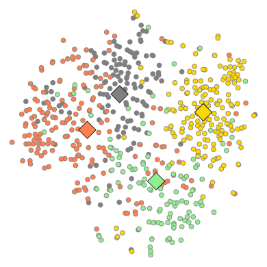
(a) without MixtFSL	(b) our MixtFSL

Figure 1: t-SNE [44] visualization of a single base class embedding (circles) (a) without, and (b) with our MixtFSL approach. MixtFSL learns a representation for base samples (circles) and associated mixture learned components (diamonds) that clusters a class into several modes (different colors). This more flexible representation helps in training robust classifiers from few samples in the novel domain compared to the monolithic representation of (a). Embeddings are extracted from a miniImageNet with a ResNet-18.

Our contributions are as follows. We introduce the idea of MixtFSL for few-shot image classification, which learns a flexible representation by modeling base classes as a mixture of learnable components. We present a robust two-stage scheme for training such a model. The training is done end-to-end in a fully differentiable fashion, without the need for an offline clustering method. We demonstrate, through an extensive experiments on four standard datasets and using four backbones, that our MixtFSL outperforms the state of the art in most of the cases tested. We show that our approach is flexible and can leverage other improvements in the literature (we experiment with associative alignment [1] and ODE [82]) to further boost performance. Finally, we show that our approach does not suffer from forgetting (the base classes).

2 Related work

Few-shot learning is now applied to problems such as image-to-image translation [76], object detection [14, 50], video classification  [6], and 3D shape segmentation [75]. This paper instead focuses on the image classification problem [18, 64, 73], so the remainder of the discussion will focus on relevant works in this area. In addition, unlike transductive inference methods [4, 12, 30, 32, 33, 43, 90, 52] which uses the structural information of the entire novel set, our research focuses on inductive inference research area.

Meta learning  In meta learning [12, 18, 55, 59, 63, 64, 65, 72, 79, 83], approaches imitate the few-shot scenario by repeatedly sampling similar scenarios (episodes) from the base classes during the pre-training phase. Here, distance-based approaches [3, 21, 34, 39, 40, 49, 64, 67, 70, 73, 80, 84, 87] aim at transferring the reduced intra-class variation from base to novel classes, while initialization-based approaches [18, 19, 35] are designed to carry the best starting model configuration for novel class training. Our MixtFSL benefits from the best of both worlds, by reducing the within-class distance with the learnable mixture component and increasing the adaptivity of the network obtained after initial training by representing each class with mixture components.

Standard transfer learning  Batch form training makes use of a standard transfer learning modus operandi instead of episodic training. Although batch learning with a naive optimization criteria is prone to overfitting, several recent studies [1, 8, 24, 51, 69] have shown a metric-learning (margin-based) criteria can offer good performance. For example, Bin et al. [41] present a negative margin based feature space learning. Our proposed MixtFSL also uses transfer learning but innovates by simultaneously clustering base class features into multi-modal mixtures in an online manner.

Data augmentation  Data augmentation [9, 10, 20, 23, 25, 27, 42, 45, 57, 60, 77, 78, 85, 86, 88] for few-shot image classification aims at training a well-generalized algorithm. Here, the data can be augmented using a generator function. For example, [27] proposed Feature Hallucination (FH) using an auxiliary generator. Later, [77] extends FH to generate new data using generative models. In contrast, our MixtFSL does not generate any data and achieves state-of-the-art. [1] makes use of “related base” samples in combination with an alignment technique to improve performance. We demonstrate (in sec. 6) that we can leverage this approach in our framework since our contribution is orthogonal.

Mixture modeling  Similar to classical mixture-based works [17, 22] outside few-shot learning, infinite mixture model [29] explores Bayesian methods [54, 81] to infer the number of mixture components. Recently, IMP [2] relies on the DP-means [36] algorithm which is computed inside the episodic training loop in few-shot learning context. As in [29], our MixtFSL automatically learns the number of mixture components, but differs from [2] by learning the mixture model simultaneously with representation learning in an online manner, without the need for a separate, post hoc clustering algorithm. From the learnable component perspective, our MixtFSL is related to VQ-VAE [56, 71] which learns quantized feature vectors for image generation, and SwAV [7] for self-supervised learning. Here, we tackle supervised few-shot learning by using mixture modeling to increase the adaptivity of the learned representation. This also contrasts with variational few-shot learning [34, 87], which aims to reduce noise with variational estimates of the distribution. Our MixtFSL is also related to MM-Net [5] in that they both works store information during training. Unlike MM-Net, which contains read/write controllers plus a contextual learner to build an attention-based inference, our MixtFSL aims at modeling the multi-modality of the base classes with only a set of learned components.

3 Problem definition

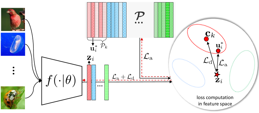
Figure 2: Initial training stage. The network $f(\cdot|\theta)$ embeds a batch (left) from the base classes to feature space. A feature vector $\mathbf{z}_{i}$ (middle) belonging to the $k$-th class is assigned to the most similar component $\mathbf{u}^{*}_{i}$ in class mixture $\mathcal{P}_{k}\in\bm{\mathcal{P}}$. Vectors are color-coded by class. Here, two losses interact for representation learning: $\mathcal{L}_{\mathrm{a}}$ which maximizes the similarity between $\mathbf{z}_{i}$ and $\mathbf{u}^{*}_{i}$; and $\mathcal{L}_{\mathrm{d}}$ keeps $\mathbf{z}_{i}$ close to the centroid $\mathbf{c}_{k}$ of all mixture components for class $k$. The backpropagated gradient is shown with red dashed lines. While $f(\cdot|\theta)$ is updated by $\mathcal{L}_{\mathrm{it}}$ (eq. 5), $\bm{\mathcal{P}}$ is updated by $\mathcal{L}_{\mathrm{a}}$ only to prevent collapsing of the components in $\mathcal{P}_{k}$ to a single point.

In few-shot image classification, we assume there exists a “base” set $\mathcal{X}^{b}=\{(\mathbf{x}_{i},y_{i})\}_{i=1}^{N^{b}}$, where $\mathbf{x}_{i}\in\mathbb{R}^{D}$ and $y_{i}\in\mathcal{Y}^{b}$ are respectively the $i$-th input image and its corresponding class label. There is also a “novel” set $\mathcal{X}^{n}=\{(\mathbf{x}_{i},y_{i})\}_{i=1}^{N^{n}}$, where $y_{i}\in\mathcal{Y}^{n}$, and a “validation” set $\mathcal{X}^{v}=\{(\mathbf{x}_{i},y_{i})\}_{i=1}^{N^{v}}$, where $y_{i}\in\mathcal{Y}^{v}$. None of these sets overlap and $N^{n}\ll N^{b}$.

In this paper, we follow the standard transfer learning training strategy (as in, for example, [1, 8]). A network $\mathbf{z}=f(\mathbf{x}|\theta)$, parameterized by $\theta$, is pre-trained to project input image $\mathbf{x}$ to a feature vector $\mathbf{z}\in\mathbb{R}^{M}$ using the base categories $\mathcal{X}^{b}$, validated on $\mathcal{X}^{v}$. The key idea behind our proposed MixtFSL model is to simultaneously train a learnable mixture model, along with $f(\cdot|\theta)$, in order to capture the distribution of each base class in $\mathcal{X}^{b}$. This mixture is guiding the representation learning for a better handling of multimodal class distributions, while allowing to extract information on the base class components that can be useful to stabilize the training. We denote the mixture model across all base classes as the set $\bm{\mathcal{P}}=\{(\mathcal{P}_{k},y_{k})\}_{k=1}^{N^{b}}$, where each $\mathcal{P}_{k}=\{\mathbf{u}_{j}\}_{j=1}^{N^{k}}$ is the set of all $N^{k}$ components $\mathbf{u}_{j}\in\mathbb{R}^{M}$ assigned to the $k$-th base class. After training on the base categories, fine-tuning the classifier on the novel samples is very simple and follows [8]: the weights $\theta$ are fixed, and a single linear classification layer $\mathbf{W}$ is trained as in $c(\cdot|\mathbf{W})\equiv\mathbf{W}^{\top}f(\cdot|\theta)$, followed by softmax. The key observation is that the mixture model, trained only on the base classes, makes the learned feature space more discriminative—only a simple classification layer can thus be trained on the novel classes.

4 Mixture-based Feature Space Learning

Data: feature extractor $f(\cdot|{\theta})$, mixture $\bm{\mathcal{P}}$, base dataset $\mathcal{X}^{b}$, validation dataset $\mathcal{X}^{v}$, maximum epoch $\alpha_{0}$, patience $\alpha_{1}$, and error evaluation function $E(\cdot)$

Result: Model $f(\cdot|{\theta^{\mathrm{best}}})$ and mixture $\bm{\mathcal{P}}^{\mathrm{best}}$ learned

$\theta^{\mathrm{best}}\leftarrow\theta$; $\bm{\mathcal{P}}^{\mathrm{best}}\leftarrow\bm{\mathcal{P}}$; $t\leftarrow 0$; $s\leftarrow 0$

while $s<\alpha_{0}\text{ and }t<\alpha_{1}$ do

       for $(\mathbf{x}_{i},y_{i})\in\mathcal{X}^{b}$ do

             Evaluate $\mathbf{z}_{i}\leftarrow f(\mathbf{x}_{i}|\theta)$, and $\mathbf{u}^{*}_{i}$ by eq. 2

             Update weights $\theta$ and mixture $\bm{\mathcal{P}}$ with $\mathcal{L}_{\mathrm{it}}$ (eq. 5);

       end for

      Evaluate $f(\cdot|{\theta})$ on $\mathcal{X}^{v}$ with episodic training

       if $E(\theta,\bm{\mathcal{P}}|\mathcal{X}^{v})<E(\theta^{\mathrm{best}},\bm{\mathcal{P}}^{\mathrm{best}}|\mathcal{X}^{v})$ then

             $\theta^{\mathrm{best}}\leftarrow\theta$; $\bm{\mathcal{P}}^{\mathrm{best}}\leftarrow\bm{\mathcal{P}}$; $t\leftarrow 0$

      else

             $t\leftarrow t+1$

       end if

      $s\leftarrow s+1$

end while

Algorithm 1 Initial training.

Training our MixtFSL on the base classes is done in two main stages: initial training and progressive following.

4.1 Initial training

The initial training of the feature extractor $f(\cdot|\theta)$ and the learnable mixture model $\bm{\mathcal{P}}$ from the base class set $\mathcal{X}^{b}$ is detailed in algorithm 1 and illustrated in fig. 2. In this stage, model parameters are updated using two losses: the “assignment” loss $\mathcal{L}_{\mathrm{a}}$, which updates both the feature extractor and the mixture model such that feature vectors are assigned to their nearest mixture component; and the “diversity” loss $\mathcal{L}_{\mathrm{d}}$, which updates the feature extractor to diversify the selection of components for a given class. Let us define the following angular margin-based softmax function [11], modified with a temperature variable $\tau$:

$$p_{\theta}(v_{j}|\mathbf{z}_{i},\bm{\mathcal{P}})=$$ (1)

$$\frac{e^{\cos\left((\angle(\mathbf{z}_{i},\mathbf{u}_{j})+m)\right)/\tau}}{e^{\cos\left((\angle(\mathbf{z}_{i},\mathbf{u}_{j})+m)\right)/\tau}+\sum\limits_{\mathbf{u}_{l}\in\{\bm{\mathcal{P}}\backslash\mathbf{u}_{j}\}}e^{\cos\left(\angle(\mathbf{z}_{i},\mathbf{u}_{l})\right)/\tau}}\,,$$

where, $m$ is a margin; $v_{j}$ is the pseudo-label associated to $\mathbf{u}_{j}$; and, $\angle(\mathbf{z}_{i},\mathbf{u}_{j})=\arccos\left(\mathbf{z}_{i}^{\top}\mathbf{u}_{i}/(||\mathbf{z}_{i}||||\mathbf{u}_{j}||)\right)$.

Given a training image $\mathbf{x}_{i}$ from base class $y_{i}=k$ and its associated feature vector $\mathbf{z}_{i}=f(\mathbf{x}_{i}|\theta)$, the closest component $\mathbf{u}^{*}_{i}$ is found amongst all elements of mixture $\mathcal{P}_{k}$ associated to the same class according to cosine similarity:

$$\mathbf{u}_{i}^{*}=\operatorname*{arg\,max}_{\mathbf{u}_{j}\in\mathcal{P}_{k}}\frac{\mathbf{z}_{i}\cdot\mathbf{u}_{j}}{\|\mathbf{z}_{i}\|\|\mathbf{u}_{j}\|}\,,$$ (2)

where $\cdot$ denotes the dot product.

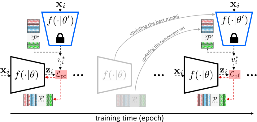
Figure 3: Progressive following training stage. $f(\cdot|\theta)$ is adapted using loss function $\mathcal{L}_{\mathrm{pf}}$ (eq. 7) and supervised by a fixed copy of the best target model $f(\cdot|\theta^{\prime})$ (in blue) and the corresponding mixture $\bm{\mathcal{P}}^{\prime}$ after the initial training stage. The gradient (dashed red line) is backpropagated only through $f(\cdot|\theta)$ and $\bm{\mathcal{P}}$, while $f(\cdot|\theta^{\prime})$ and $\bm{\mathcal{P}}^{\prime}$ are kept fixed. The target network and mixture $f(\cdot|\theta^{\prime})$ and $\bm{\mathcal{P}}^{\prime}$ are replaced by the best validated $f(\cdot|\theta)$ and $\mathcal{P}$ after $\alpha_{3}$ number of training steps with no improvement in validation. The temperature factor $\tau$ (eq. 1) decreases each time the target network is updated to create progressively more discriminative clusters.

Data: pre-trained $f(\cdot|{\theta})$, pre-trained $\bm{\mathcal{P}}$, base set $\mathcal{X}^{b}$, validation set $\mathcal{X}^{v}$, patience $\alpha_{2}$, number of repetitions $\alpha_{3}$, temperature $\tau$, decreasing ratio $\gamma$, and error evaluation function $E(\cdot)$

Result: Refined model $f(\cdot|\theta^{\textrm{best}})$ and mixture $\bm{\mathcal{P}}^{\textrm{best}}$

$\theta^{\prime}\leftarrow\theta$; $\bm{\mathcal{P}}^{\prime}\leftarrow\bm{\mathcal{P}}$; $\theta^{\textrm{best}}\leftarrow\theta$; $\bm{\mathcal{P}}^{\textrm{best}}\leftarrow\bm{\mathcal{P}}$; $s\leftarrow 0$

for $t=1,2,\ldots,\alpha_{3}$ do

       while $s<\alpha_{2}$ do

             for $(\mathbf{x}_{i},\mathbf{y}_{i})\in\mathcal{X}^{b}$ do

                   Evaluate $\mathbf{z}_{i}\leftarrow f(\mathbf{x}_{i}|\theta^{\prime})$ , and $\mathbf{u}_{i}^{*}{}^{\prime}$ by eq. 6

                   Update weights $\theta$ and mixture $\bm{\mathcal{P}}$ by backward error propagation from $\mathcal{L}_{\mathrm{pf}}$ (eq. 7)

                  

             end for

            if $E(\theta,\bm{\mathcal{P}}|\mathcal{X}^{v})<E(\theta^{\mathrm{best}},\bm{\mathcal{P}}^{\mathrm{best}}|\mathcal{X}^{v})$ then

                   $\theta^{\textrm{best}}\leftarrow\theta$; $\bm{\mathcal{P}}^{\textrm{best}}\leftarrow\bm{\mathcal{P}}$; $s\leftarrow 0$

            else

                   $s\leftarrow s+1$

             end if

            

       end while

      Update target $\theta^{\prime}\leftarrow\theta^{\textrm{best}}$ and mixture $\bm{\mathcal{P}}^{\prime}\leftarrow\bm{\mathcal{P}}^{\textrm{best}}$

       Decrease temperature $\tau$ of eq. 1 as $\tau\leftarrow\gamma\tau$

      

end for

Algorithm 2 Progressive following.

Based on this, the “assignment” loss function $\mathcal{L}_{\mathrm{a}}$ updates both $f(\cdot|\theta)$ and $\bm{\mathcal{P}}$ such that $\mathbf{z}_{i}$ is assigned to its most similar component $\mathbf{u}^{*}_{i}$:

$$\mathcal{L}_{\mathrm{a}}=-\frac{1}{N}\sum_{i=1}^{N}\log p_{\theta}(v^{*}_{i}|\mathbf{z}_{i},\bm{\mathcal{P}})\,,$$ (3)

where $N$ is the batch size and $v^{*}_{i}$ is the one-hot pseudo-label corresponding to $\mathbf{u}_{i}^{*}$. The gradient of eq. 3 is back-propagated to both $f(\cdot|\theta)$ and the learned components $\bm{\mathcal{P}}$.

As verified later (sec. 5.3), training solely on the assignment loss $\mathcal{L}_{\mathrm{a}}$ generally results in a single component $\mathbf{u}_{i}\in\mathcal{P}_{k}$ to be assigned to all training instances for class $k$, thereby effectively degrading the learned mixtures to a single mode. We compensate for this by adding a second loss function to encourage a diversity of components to be selected by enforcing $f(\cdot|\theta)$ to push the $\mathbf{z}_{i}$ values towards the centroid of the components corresponding to their associated labels $y_{i}$. For the centroid $\bm{c}_{k}=({1}/{|\mathcal{P}_{k}|})\sum_{\mathbf{u}_{j}\in\mathcal{P}_{k}}\mathbf{u}_{j}$ for base class $k$, and the set $\bm{\mathcal{C}}=\{\bm{c}_{k}\}_{k=1}^{N^{b}}$ of the centroids for base classes, we define the diversity loss as:

$$\mathcal{L}_{\mathrm{d}}=-\frac{1}{N}\sum_{i=1}^{N}\log p_{\theta}(y_{i}|\mathbf{z}_{i},\mathrm{sg}[\bm{\mathcal{C}}])\,,$$ (4)

where $\mathrm{sg}$ stands for stopgradient, which blocks backpropagation over the variables it protects. The $\mathrm{sg}$ operator in eq. 4 prevents the collapsing of all components of the $k$-th class $\mathcal{P}_{k}$ into a single point. Overall, the loss in this initial stage is the combination of eqs 3 and 4:

$$\mathcal{L}_{\mathrm{it}}=\mathcal{L}_{\mathrm{a}}+\mathcal{L}_{\mathrm{d}}\,.$$ (5)

4.2 Progressive following

After the initial training of the feature extractor $f(\cdot|\theta)$ and mixture $\bm{\mathcal{P}}$, an intense competition is likely to arise for the assignment of the nearest components to each instance $\mathbf{z}_{i}$. To illustrate this, suppose $\mathbf{\dot{u}}$ is assigned to $\mathbf{z}$ at iteration $t$. At the following iteration $t+1$, the simultaneous weight update to both $f(\cdot|\theta)$ and $\bm{\mathcal{P}}$ could cause another ${\mathbf{\ddot{u}}}$, in the vicinity of $\mathbf{\dot{u}}$ and $\mathbf{z}$, to be assigned as the nearest component of $\mathbf{z}$. Given the margin-based softmax (eq. 1), $\mathbf{z}$ is pulled toward $\mathbf{\dot{u}}$ and pushed away from $\mathbf{\ddot{u}}$ at iteration $t$, and contradictorily steered in the opposite direction at the following iteration. As a result, this “pull-push” behavior stalls the improvement of $f(\cdot|\theta)$, preventing it from making further progress.

To tackle this problem, we propose a progressive following stage that aim to break the complex dynamic of simultaneously determining nearest components while training the representation $f(\cdot|\theta)$ and mixture $\bm{\mathcal{P}}$. The approach is detailed in algorithm 2 and shown in fig. 3. Using the “prime” notation ($\theta^{\prime}$ and $\bm{\mathcal{P}}^{\prime}$ to specify the best feature extractor parameters and mixture component so far, resp.), the approach starts by taking a copy of $f(\cdot|\theta^{\prime})$ and $\bm{\mathcal{P}}^{\prime}$, and by using them to determine the nearest component of each training instance:

$$\mathbf{u}{{}_{i}^{*}}^{\prime}=\operatorname*{arg\,max}_{\mathbf{u}_{j}^{\prime}\in\mathcal{P}_{k}^{\prime}}\frac{\mathbf{z}^{\prime}_{i}\cdot\mathbf{u}_{j}^{\prime}}{\|\mathbf{z}^{\prime}_{i}\|\|\mathbf{u}_{j}^{\prime}\|}\,,$$ (6)

where $\mathbf{z}^{\prime}_{i}=f(\mathbf{x}_{i}|\theta^{\prime})$. Since determining the labels does not depend on the learned parameters $\theta$ anymore, consistency in the assignment of nearest components is preserved, and the “push-pull” problem mentioned above is eliminated.

Since label assignments are fixed, the diversity loss (eq. 4) is not needed anymore. Therefore, we can reformulate the progressive assignment loss function as:

$$\mathcal{L}_{\mathrm{pf}}=-\frac{1}{N}\sum_{i=1}^{N}\log p_{\theta}({v_{i}^{*}}^{\prime}|\mathbf{z}_{i},\bm{\mathcal{P}})\,,$$ (7)

where $N$ is the batch size and $v{{}_{i}^{*}}^{\prime}$ the pseudo-label associated to the nearest component $\mathbf{u}{{}_{i}^{*}}^{\prime}$ found by eq. 6.

After $\alpha_{2}$ updates to the representation with no decrease of the validation set error (function $E(\cdot)$ in algorithms 1 and 2), the best network $f(\cdot|\theta^{\prime})$ and mixture $\bm{\mathcal{P}}^{\prime}$ are then replaced with the new best ones found on validation set, the temperature $\tau$ is decreased by a factor $\gamma<1$ to push the $\mathbf{z}$ more steeply towards their closest mixture component, and the entire procedure is repeated as shown in algorithm 2. After a maximum number of $\alpha_{3}$ iterations is reached, the global best possible model $\theta^{\textrm{best}}$ and mixture ${\mathcal{P}}^{\textrm{best}}$ are obtained. Components that have no base class samples associated (i.e. never selected by eq. 6) are simply discarded. This effectively adapts the mixture models to each base class distribution.

In summary, the progressive following aims at solving the discussed pull-push behavior observed (see sec. 5.3). This stage applies a similar approach than in initial stage, with two significant differences: 1) the diversity loss $\mathcal{L}_{\mathrm{d}}$ is removed; and 2) label assignments are provided by a copy of the best model so far $f(\cdot|\theta^{\prime})$ to stabilize the training.

Table 1: Evaluation on miniImageNet in 5-way. Bold/blue is best/second, and $\pm$ is the 95% confidence intervals in 600 episodes.

Method	Backbone	1-shot	5-shot
ProtoNet [64]	Conv4	49.42 $\pm$ 0.78	68.20 $\pm$ 0.66
MAML [19]	Conv4	48.07 $\pm$ 1.75	63.15 $\pm$ 0.91
RelationNet [67]	Conv4	50.44 $\pm$ 0.82	65.32 $\pm$ 0.70
Baseline++ [8]	Conv4	48.24 $\pm$ 0.75	66.43 $\pm$ 0.63
IMP [2]	Conv4	49.60 $\pm$ 0.80	68.10 $\pm$ 0.80
MemoryNetwork [5]	Conv4	53.37 $\pm$ 0.48	66.97 $\pm$ 0.35
Arcmax [1]	Conv4	51.90 $\pm$0.79	69.07 $\pm$ 0.59
Neg-Margin [41]	Conv4	52.84 $\pm$0.76	70.41 $\pm$0.66
MixtFSL (ours)	Conv4	52.82 $\pm$0.63	70.67 $\pm$0.57
DNS [62]	RN-12	62.64 $\pm$0.66	78.83 $\pm$0.45
Var.FSL [87]	RN-12	61.23 $\pm$0.26	77.69 $\pm$0.17
MTL [66]	RN-12	61.20 $\pm$1.80	75.50 $\pm$0.80
SNAIL [46]	RN-12	55.71 $\pm$0.99	68.88 $\pm$0.92
AdaResNet [48]	RN-12	56.88 $\pm$0.62	71.94 $\pm$0.57
TADAM [49]	RN-12	58.50 $\pm$0.30	76.70 $\pm$0.30
MetaOptNet [37]	RN-12	62.64 $\pm$0.61	78.63 $\pm$0.46
Simple [69]	RN-12	62.02 $\pm$0.63	79.64 $\pm$0.44
TapNet [83]	RN-12	61.65 $\pm$0.15	76.36 $\pm$0.10
Neg-Margin [41]	RN-12	63.85 $\pm$0.76	81.57 $\pm$0.56
MixtFSL (ours)	RN-12	63.98 $\pm$0.79	82.04 $\pm$0.49
MAML‡ [18]	RN-18	49.61 $\pm$0.92	65.72 $\pm$0.77
RelationNet‡ [67]	RN-18	52.48 $\pm$0.86	69.83 $\pm$0.68
MatchingNet‡ [73]	RN-18	52.91 $\pm$0.88	68.88 $\pm$0.69
ProtoNet‡ [64]	RN-18	54.16 $\pm$0.82	73.68 $\pm$0.65
Arcmax [1]	RN-18	58.70 $\pm$0.82	77.72 $\pm$0.51
Neg-Margin [41]	RN-18	59.02 $\pm$0.81	78.80 $\pm$0.54
MixtFSL (ours)	RN-18	60.11 $\pm$0.73	77.76 $\pm$0.58
Act. to Param. [53]	RN-50	59.60 $\pm$0.41	73.74 $\pm$0.19
SIB-inductive§[31]	WRN	60.12	78.17
SIB+IFSL [68]	WRN	63.14 $\pm$3.02	80.05 $\pm$1.88
LEO [59]	WRN	61.76 $\pm$0.08	77.59 $\pm$0.12
wDAE [25]	WRN	61.07 $\pm$0.15	76.75 $\pm$0.11
CC+rot [23]	WRN	62.93 $\pm$0.45	79.87 $\pm$0.33
Robust dist++ [13]	WRN	63.28 $\pm$0.62	81.17 $\pm$0.43
Arcmax [1]	WRN	62.68 $\pm$0.76	80.54 $\pm$0.50
Neg-Margin [41]	WRN	61.72 $\pm$0.90	81.79 $\pm$0.49
MixtFSL (ours)	WRN	64.31 $\pm$0.79	81.66 $\pm$0.60

^‡taken from [8]  ^§confidence interval not provided

5 Experimental validation

The following section presents the experimental validations of our novel mixture-based feature space learning (MixtFSL). We begin by introducing the datasets, backbones and implementation details. We then present experiments on object recognition, fine-grained and cross-domain classification. Finally, an ablative analysis is presented to evaluate the impact of decisions made in the design of MixtFSL.

5.1 Datasets and implementation details

Datasets  Object recognition is evaluated using the miniImageNet [73] and tieredImageNet [57], which are subsets of the ILSVRC-12 dataset [58]. miniImageNet contains 64/16/20 base/validation/novel classes respectively with 600 examples per class, and tieredImageNet [57] contains 351/97/160 base/validation/novel classes. For fine-grained classification, we employ CUB-200-2011 (CUB) [74] which contains 100/50/50 base/validation/novel classes. For cross-domain, we train on the base and validation classes of miniImageNet, and evaluate on the novel classes of CUB.

Backbones and implementation details  We conduct experiments using four different backbones: 1) Conv4, 2) ResNet-18 [28], 3) ResNet-12 [28], and 4) 28-layer Wide-ResNet (“WRN”) [61]. We used Adam [49] and SGD with a learning rate of $10^{-3}$ to train Conv4 and ResNets and WRN, respectively. In SGD case, we used Nesterov with an initial rate of 0.001, and the weight decay is fixed as 5e-4 and momentum as 0.9. In all cases, batch size is fixed to 128. The starting temperature variable $\tau$ and margin $m$ (eq. 1 in sec. 4) were found using the validation set (see supp. material). Components in $\bm{\mathcal{P}}$ are initialized with Xavier uniform [26] ($\text{gain}=1$), and their number $N^{k}=15$ (sec. 3), except for tieredImageNet where $N^{k}=5$ since there is a much larger number of bases classes (351). A temperature factor of $\gamma=0.8$ is used in the progressive following stage. The early stopping thresholds of algorithms 1 and 2 are set to $\alpha_{0}=400$, $\alpha_{1}=20$, $\alpha_{2}=15$ and $\alpha_{3}=3$.

Table 2: Evaluation on tieredImageNet and FC100 in 5-way classification. Bold/blue is best/second best, and $\pm$ indicates the 95% confidence intervals over 600 episodes.

	Method	Backbone	1-shot	5-shot
tieredImageNet	DNS [62]	RN-12	66.22 $\pm$0.75	82.79 $\pm$0.48
	MetaOptNet [37]	RN-12	65.99 $\pm$0.72	81.56 $\pm$0.53
	Simple [69]	RN-12	69.74 $\pm$0.72	84.41 $\pm$0.55
	TapNet [83]	RN-12	63.08 $\pm$0.15	80.26 $\pm$0.12
	Arcmax∗ [1]	RN-12	68.02 $\pm$0.61	83.99 $\pm$0.62
	MixtFSL (ours)	RN-12	70.97 $\pm$1.03	86.16 $\pm$0.67
	Arcmax [1]	RN-18	65.08 $\pm$0.19	83.67 $\pm$0.51
	ProtoNet [64]	RN-18	61.23 $\pm$0.77	80.00 $\pm$0.55
	MixtFSL (ours)	RN-18	68.61 $\pm$0.91	84.08 $\pm$0.55
FC100	TADAM [49]	RN-12	40.1 $\pm$ 0.40	56.1 $\pm$ 0.40
	MetaOptNet [37]	RN-12	41.1 $\pm$ 0.60	55.5 $\pm$ 0.60
	ProtoNet† [64]	RN-12	37.5 $\pm$ 0.60	52.5 $\pm$ 0.60
	MTL [66]	RN-12	43.6 $\pm$ 1.80	55.4 $\pm$ 0.90
	MixtFSL (ours)	RN-12	44.89 $\pm$0.63	60.70 $\pm$0.67
	Arcmax [1]	RN-18	40.84 $\pm$ 0.71	57.02 $\pm$ 0.63
	MixtFSL (ours)	RN-18	41.50 $\pm$0.67	58.39 $\pm$0.62

^∗our implementation  ^†taken from [37]

5.2 Mixture-based feature space evaluations

We first evaluate our proposed MixtFSL model on all four datasets using a variety of backbones.

miniImageNet  Table 1 compares our MixtFSL with several recent method on miniImageNet, with four backbones. MixtFSL provides accuracy improvements in all but three cases. In the most of these exceptions, the method with best accuracy is Neg-Margin [41], which is explored in more details in sec. 6. Of note, MixtFSL outperforms IMP [2] (sec. 1 and 2) by 3.22% and 2.57% on 1- and 5-shot respectively, thereby validating the impact of jointly learning the feature representation together with the mixture model.

tieredImageNet and FC100  Table 2 presents similar comparisons, this time on tieredImageNet and FC100. On both datasets and in both 1- and 5-shot scenarios, our method yields state-of-the-art results. In particular, MixtFSL results in classification gains of 3.53% over Arcmax [1] in 1-shot using RN-18, and 1.75% over Simple [69] in 5-shot using ResNet-12 for tieredImageNet, and 1.29% and 4.60% over MTL [66] for FC100 in 1- and 5-shot, respectively.

CUB  Table 3 evaluates our approach on CUB, both for fine-grained classification in 1- and 5-shot, and in cross-domain from miniImageNet to CUB for 5-shot using the ResNet-18. Here, previous work [41] outperforms MixtFSL in the 5-shot scenario. We hypothesize this is due to the fact that either CUB classes are more unimodal than miniImageNet or that less examples per-class are in the dataset, which could be mitigated with self-supervised methods.

Table 3: Fine-grained and on cross-domain from miniImageNet to CUB evaluation in 5-way using ResNet-18. Bold/blue is best/second, and $\pm$ is the 95% confidence intervals on 600 episodes.

	CUB		miniIN$\xrightarrow{}$CUB
Method	1-shot	5-shot	5-shot
GNN-LFT⋄ [70]	51.51 $\pm$0.8	73.11 $\pm$0.7	–
Robust-20 [13]	58.67 $\pm$0.7	75.62 $\pm$0.5	–
RelationNet‡ [67]	67.59 $\pm$1.0	82.75 $\pm$0.6	57.71 $\pm$0.7
MAML‡ [18]	68.42 $\pm$1.0	83.47 $\pm$0.6	51.34 $\pm$0.7
ProtoNet‡ [64]	71.88 $\pm$0.9	86.64 $\pm$0.5	62.02 $\pm$0.7
Baseline++ [8]	67.02 $\pm$0.9	83.58 $\pm$0.5	64.38 $\pm$0.9
Arcmax [1]	71.37 $\pm$0.9	85.74 $\pm$0.5	64.93 $\pm$1.0
Neg-Margin [41]	72.66 $\pm$0.9	89.40 $\pm$0.4	67.03 $\pm$0.8
MixtFSL (ours)	73.94 $\pm$1.1	86.01 $\pm$0.5	68.77 $\pm$0.9

^‡taken from [68]  ^⋄backbone is ResNet-10

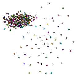
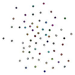
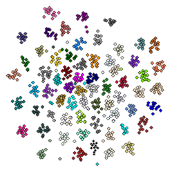
(a) without $\mathcal{L}_{d}$	(b) $\mathcal{L}_{d}$ without $\mathrm{sg}$	(c) $\mathcal{L}_{d}$ with $\mathrm{sg}$

Figure 4: t-SNE of mixture components (RN-12, miniImageNet).

5.3 Ablative analysis

Here, we perform ablative experiments to evaluate the impact of two design decisions in our approach.

Initial training vs progressive following  Fig. 4 illustrates the impact of loss functions qualitatively. Using only $\mathcal{L}_{\mathrm{a}}$ causes a single component to dominate while the others are pushed far away (big clump in fig. 4a) and is equivalent to the baseline (table 4, rows 1–2). Adding $\mathcal{L}_{\mathrm{d}}$ without the $\mathrm{sg}$ operator minimizes the distance between the $\mathbf{z}_{i}$’s to the centroids, resulting in the collapse of all components in $\mathcal{P}_{k}$ into a single point (fig. 4b). $\mathrm{sg}$ prevents the components (through their centroids) from being updated (fig. 4c), which results in improved performance in the novel domain (t. 4, row 3). Finally, $\mathcal{L}_{\mathrm{pf}}$ further improves performance while bringing stability to the training (t. 4, row 4). Beside, Fig. 5 presents a t-SNE [44] visualization of base examples and their associated mixture components. Compared to initial training, the network at the end of progressive following stage results in an informative feature space with the separated base classes.

Diversity loss $\mathcal{L}_{\mathrm{d}}$  Fig. 6 presents the impact of our diversity loss $\mathcal{L}_{\mathrm{d}}$ (eq. 4) by showing the number of remaining components after optimization (recall from sec. 4.2 that components assigned to no base sample are discarded after training). Without $\mathcal{L}_{\mathrm{d}}$ (fig. 6a), most classes are represented by a single component. Activating $\mathcal{L}_{\mathrm{d}}$ results in a large number of components having non-zero base samples, thereby results in the desired mixture modeling (fig. 6b).

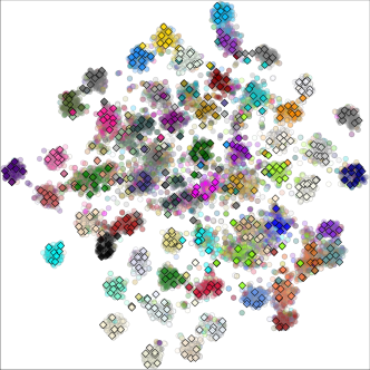
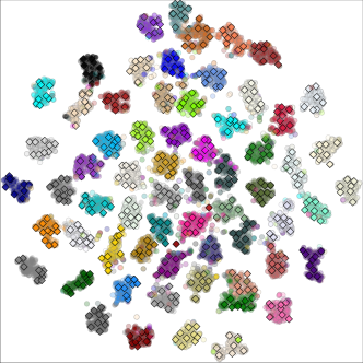
(a) after initial training	(b) after progressive following

Figure 5: t-SNE [44] visualization of the learned feature embedding (circles) and mixture components (diamonds), after the (a) initial training and (b) progressive following stages. Results are obtained with the ResNet-12 and points are color-coded by base class.

Table 4: Validation set accuracy of miniImageNet on 150 epochs.

	RN-12		RN-18
Method	1-shot	5-shot	1-shot	5-shot
Baseline	56.55	72.68	55.38	72.81
Only $\mathcal{L}_{\mathrm{a}}$	56.52	72.78	55.55	72.67
Init. tr. ($\mathcal{L}_{\mathrm{a}}+\mathcal{L}_{\mathrm{d}}$)	57.88	73.94	56.18	69.43
Prog. fol. ($\mathcal{L}_{\mathrm{a}}+\mathcal{L}_{\mathrm{d}}+\mathcal{L}_{\mathrm{pf}}$)	58.60	76.09	57.91	73.00

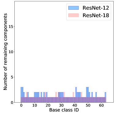
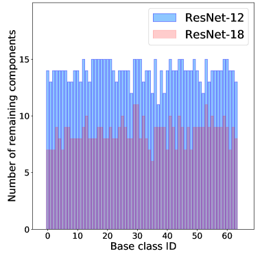
(a) without $\mathcal{L}_{\mathrm{d}}$	(b) with $\mathcal{L}_{\mathrm{d}}$

Figure 6: Number of remaining components after training for each of the miniImageNet base classes (a) without and (b) with the diversity loss $\mathcal{L}_{\mathrm{d}}$ (eq. 4) using ResNet-12 and ResNet-18. The loss is critical to model the multimodality of base classes.

Margin in eq. 1  As in [1] and [41], our loss function (eq. 1) uses a margin-based softmax function modulated by a temperature variable $\tau$. In particular, [41] suggested that a negative margin $m<0$ improves accuracy. Here, we evaluate the impact of the margin $m$, and demonstrate in table 5 that MixtFSL does not appear to be significantly affected by its sign.

Table 5: Margin ablation using miniImageNet in 5-way classification. Bold/blue is best/second best, and $\pm$ indicates the 95% confidence intervals over 600 episodes.

Method	Backbone	1-shot	5-shot
MixtFSL-Neg-Margin	RN-12	63.98 $\pm$0.79	82.04 $\pm$0.49
MixtFSL-Pos-Margin	RN-12	63.57 $\pm$0.00	81.70 $\pm$0.49
MixtFSL-Neg-Margin	RN-18	60.11 $\pm$0.73	77.76 $\pm$0.58
MixtFSL-Pos-Margin	RN-18	59.71 $\pm$0.76	77.59 $\pm$0.58

6 Extensions

We present extensions of our approach that make use of two recent works: the associative alignment of Afrasiyabi et al. [1], and Ordinary Differential Equation (ODE) of Xu et al. [82]. In both cases, employing their strategies within our framework yields further improvements, demonstrating the flexibility of our MixtFSL.

6.1 Associative alignment [1]

Two changes are necessary to adapt our MixtFSL to exploit the “centroid alignment” of Afrasiyabi et al. [1]. First, we employ the learned mixture model $\bm{\mathcal{P}}$ to find the related base classes. This is both faster and more robust than [1] who rely on the base samples themselves. Second, they used a classification layer $\mathbf{W}$ in $c(\mathbf{x}|\mathbf{W})\equiv\mathbf{W}^{\top}f(\mathbf{x}|\theta)$ (followed by softmax). Here, we use two heads ($\mathbf{W}^{b}$ and $\mathbf{W}^{n}$), to handle base and novel classes separately.

Table 6: Comparison of our MixtFSL with alignment (MixtFSL-Align) in 5-way classification. Here, bold is the best performance.

	Method	Backbone	1-shot	5-shot
miniIN	Cent. Align.∗ [1]	RN-12	63.44 $\pm$0.67	80.96 $\pm$0.61
	MixtFSL-Align. (ours)	RN-12	64.38 $\pm$0.73	82.45 $\pm$0.62
	Cent. Align.∗ [1]	RN-18	59.85 $\pm$0.67	80.62 $\pm$0.72
	MixtFSL-Align. (ours)	RN-18	60.44 $\pm$1.02	81.76 $\pm$0.74
tieredIN	Cent. Align.∗ [1]	RN-12	71.08 $\pm$0.93	86.32 $\pm$0.66
	MixtFSL-Align. (ours)	RN-12	71.83 $\pm$0.99	88.20 $\pm$0.55
	Cent. Align.∗ [1]	RN-18	69.18 $\pm$0.86	85.97 $\pm$0.51
	MixtFSL-Align. (ours)	RN-18	69.82 $\pm$0.81	85.57 $\pm$0.60

^∗ our implementation

Evaluation  We evaluate our adapted alignment algorithm on the miniImageNet and tieredImageNet using the RN-18 and RN-12. Table 6 presents our MixtFSL and MixtFSL-alignment (MixtFSL-Align.) compared to [1] for the 1- and 5-shot (5-way) classification problems. Employing MixtFSL improves over the alignment method of [1] in all cases except in 5-shot (RN-18) on tieredImageNet, which yields slightly worse results. However, our MixtFSL results in gain up to 1.49% on miniImageNet and 1.88% on tieredImageNet (5-shot, RN-12). To ensure a fair comparison, we reimplemented the approach proposed in [1] using our framework.

Forgetting  Aligning base and novel examples improves classification accuracy, but may come at the cost of forgetting the base classes. Here, we make a comparative evaluation of this “remembering” capacity between our approach and that of Afrasiyabi et al. [1]. To do so, we first reserve 25% of the base examples from the dataset, and perform the entire training on the remaining 75%. After alignment, we then go back to the reserved classes and evaluate whether the trained models can still classify them accurately. Table 7 presents the results on miniImageNet. It appears that Afrasiyabi et al. [1] suffers from catastrophic forgetting with a loss of performance ranging from 22.1–33.5% in classification accuracy. Our approach, in contrast, effectively remembers the base classes with a loss of only 0.5%, approximately.

6.2 Combination with recent and concurrent works

Several recent and concurrent works [38, 89, 82, 15] present methods which achieves competitive—or even superior—performance to that of MixtFSL presented in table 1. They achieve this through improvements in neural network architectures: [38] adds a stack of 3 convolutional layers as a pre-backbone to train other modules (SElayer, CSEI and TSFM), [89] uses a pre-trained RN-12 to train a “Cross Non-local Network”, and [15] adds an attention module with 1.64M parameters to the RN-12 backbone. Xu et al. [82] also modify the RN-12 and train an adapted Neural Ordinary Differential Equation (ODE), which consists of a dynamic meta-filter and adaptive alignment modules. The aim of the extra alignment module in [82] is to perform channel-wise adjustment besides the spatial-level adaptation. In contrast to these methods, we emphasize that as opposed to these works, all MixtFSL results presented throughout the paper have been obtained with standard backbones without additional architectural changes.

Since this work focuses on representation learning, our approach is thus orthogonal—and can be combined—to other methods which contain additional modules. To support this point, table 8 combines MixtFSL with the ODE approach of Xu et al. [82] (MixtFSL-ODE) and shows that the resulting combination results in a gain of 0.85% and 1.48% over [82] in 1- and 5-shot respectively.

Table 7: Evaluation of the capacity to remember base classes before and after alignment. Evaluation performed on miniImageNet in 5-way image classification. Numbers in () indicate the change in absolute classification accuracy compared to before alignment.

Method	Backbone	1-shot	5-shot
[1] before align.	RN-12	96.17	97.49
[1] after align.	RN-12	65.47 (-30.7)	75.37 (-22.12)
ours before align.	RN-12	96.83	98.06
ours after align.	RN-12	96.27 (-0.6)	98.11 (+0.1)
[1] before align.	RN-18	91.56	90.72
[1] after align.	RN-18	58.02 (-33.5)	62.97 (-27.8)
ours before align.	RN-18	97.46	98.16
ours after align.	RN-18	97.20 (-0.3)	97.65 (-0.5)

Table 8: Combining MixtFSL with the ODE appraoch of Xu et al. [82] (MixtFSL-ODE) in 5-way on miniImageNet using RN-12.

Method	1-shot	5-shot
ODE [82]	67.76 $\pm$0.46	82.71 $\pm$0.31
MixtFSL-ODE	68.61 $\pm$0.73	84.19 $\pm$0.44

7 Discussion

This paper presents the idea of Mixture-based Feature Space Learning (MixtFSL) for improved representation learning in few-shot image classification. It proposes to simultaneously learn a feature extractor along with a per-class mixture component in an online, two-phase fashion. This results in a more discriminative feature representation yielding to superior performance when applied to the few-shot image classification scenario. Experiments demonstrate that our approach achieves state-of-the-art results with no ancillary data used. In addition, combining our MixtFSL with [1] and [82] results in significant improvements over the state of the art for inductive few-shot image classification. A limitation of our MixtFSL is the use of a two-stage training, requiring a choreography of steps for achieving strong results while possibly increasing training time. A future line of work would be to revise it into a single stage training procedure to marry representation and mixture learning, with stable instance assignment to components, hopefully giving rise to a faster and simpler mixture model learning. Another limitation is observed with small datasets where the within-class diversity is low such that the need for mixtures is less acute (cf. CUB dataset in fig. 3). Again, with a single-stage training, dealing with such a unimodal dataset may be better, allowing to activate multimodal mixtures only as required.

Acknowledgements

This project was supported by NSERC, Mitacs, Prompt-Quebec, and Compute Canada. We thank M. Tremblay, H. Weber, A. Schwerdtfeger, A. Tupper, C. Shui, C. Bouchard, and B. Leger for proofreading the manuscript, and F. N. Nokabadi for help.

In this supplementary material, the following items are provided:

1. Ablation on the number of components $N^{k}$ in the mixture model $\bm{\mathcal{P}}$ (sec. 8)

2. Dynamic of the training (sec. 9);

3. More ways ablation (sec. 10);

4. Ablation of the margin $m$ (sec. 11);

5. Ablation of the temperature $\tau$ (sec. 12);

6. Visualization: from MixtFSL to MixtFSL-Alignment (sec. 13);

8 Ablation on the number of components $N^{k}$ in the mixture model $\bm{\mathcal{P}}$

Although our proposed MixtFSL automatically infers the number of per-class mixture components from data, we also ablate the initial size of mixture model $N^{k}$ for each class to evaluate whether it has an impact on the final results. Table 9 presents 1- and 5-shot classification results on miniImageNet using ResNet-12 and ResNet-18 by initializing $N^{k}$ to 5, 10, 15, and 20 components per class.

Initializing $N^{k}=5$ results in lower classification accuracy compared to the higher $N^{k}$. We think this is possible due to the insufficient capacity of small mixture model $\bm{\mathcal{P}}$ size. However, as long as $N^{k}$ is sufficiently large (10, 15, 20), our approach is robust to this parameter and results do not change significantly as a function of $N^{k}$. Note that $N^{k}$ cannot be set to an arbitrary high number due to memory limitations.

Table 9: Classification results on mini-ImageNet using ResNet-12 and ResNet-18 backbones as a function of the initial value for the number of components per class $N^{k}$. $\pm$ denotes the $95\%$ confidence intervals over 300 episodes.

$N^{k}$ 1-shot 5-shot 5 62.29 $\pm$1.08 78.85 $\pm$0.61 10 64.01 $\pm$0.79 81.87 $\pm$0.49 15 63.98 $\pm$0.79 82.04 $\pm$0.49 20 63.91 $\pm$0.80 82.05 $\pm$0.49	$N^{k}$ 1-shot 5-shot 5 58.57 $\pm$1.09 76.44 $\pm$0.61 10 60.15 $\pm$0.80 77.71 $\pm$0.61 15 60.11 $\pm$0.73 77.76 $\pm$0.58 20 58.99 $\pm$0.81 77.77 $\pm$0.58
(a) ResNet-12	(b) ResNet-18

9 Dynamic of the training

Fig. 7 evaluates the necessity of the two training stages (sec. 4 from the main paper) by showing the (episodic) validation accuracy during 150 epochs. The vertical dashed line indicates the transition between training stages. In most cases, the progressive following stage results in a validation accuracy gain.

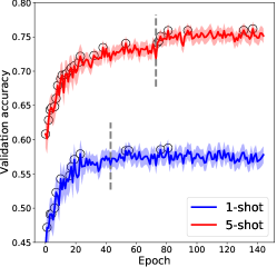
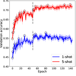
(a) ResNet-12	(b) ResNet-18

Figure 7: Validation accuracy of the first 150 epochs using ResNet-12 and ResNet-18 on miniImageNet. 1- and 5-shot scenarios are plotted using blue and red colors with their confidence intervals over 300 testing episodes of the validation set, respectively. The dashed vertical line is starting point of progressive following stage. The circles are the points when we update the best model.

10 More ways ablation

Table 10 presents more-way 5-shot comparison of our MixtFSL on miniImageNet using ResNet-18 and ResNet-12. Our MixtFSL gains 1.14% and 1.23% over the Pos-Margin [1] in 5-way and 20-way, respectively. Besides, MixtFSL gains 0.78% over Baseline++ [8] in 10-way.

We could not find “more-ways” results with the ResNet-12 backbone in the literature, but we provide our results here for potential future literature comparisons.

Table 10: $N$-way 5-shot classification results on mini-ImageNet using ResNet-18 and ResNet-12 backbones. $\pm$ denotes the $95\%$ confidence intervals over 600 episodes. The best results prior this work is highlighted in blue, and the best results are presented in boldfaced.

Method	Backbone	5-way		10-way		20-way
MatchingNet‡ [73]	RN-18	68.88 $\pm$0.69		52.27 $\pm$0.46		36.78 $\pm$0.25
ProtoNet‡ [64]	RN-18	73.68 $\pm$0.65		59.22 $\pm$0.44		44.96 $\pm$0.26
RelationNet‡ [67]	RN-18	69.83 $\pm$0.68		53.88 $\pm$0.48		39.17 $\pm$0.25
Baseline [8]	RN-18	74.27 $\pm$0.63		55.00 $\pm$0.46		42.03 $\pm$0.25
Baseline++ [8]	RN-18	75.68 $\pm$0.63		63.40 $\pm$0.44		50.85 $\pm$0.25
Pos-Margin [1]	RN-18	76.62 $\pm$0.58		62.95 $\pm$0.83		51.92 $\pm$1.02
MixtFSL (ours)	RN-18	77.76 $\pm$0.58		64.18 $\pm$0.76		53.15 $\pm$0.71
MixtFSL (ours)	RN-12	82.04 $\pm$0.49		68.26 $\pm$0.71		55.41 $\pm$0.71

^‡ implementation from [8]

11 Ablation of the margin

As table 11 shows, a negative margin provides slightly better results than using a positive one, thus replicating the findings from Liu et al. [41], albeit with a more modest improvement than reported in their paper. We theorize that the differences between our results (in table 11) and theirs are due to slight differences in training setup (e.g., learning rate scheduling, same optimizer for base and novel classes). Nevertheless, the impact of the margin on our proposed MixtFSL approach is similar. We also note that in all cases except 5-shot on ResNet-18, our proposed MixtFSL yields significant improvements. Notably, MixtFSL provides classification improvements of 2.08% and 3.18% in 1-shot and 5-shot using ResNet-12.

Table 11: Margin evaluation using miniImageNet in 5-way classification. Bold/blue is best/second best, and $\pm$ indicates the 95% confidence intervals over 600 episodes.

Method	Backbone	1-shot	5-shot
Neg-Margin∗ [41]	Conv4	51.81 $\pm$0.81	69.24 $\pm$0.59
ArcMax∗ [1]	Conv4	51.95 $\pm$0.80	69.05 $\pm$ 0.58
MixtFSL-Neg-Margin	Conv4	52.76 $\pm$0.67	70.67 $\pm$0.57
MixtFSL-Pos-Margin	Conv4	52.82 $\pm$0.63	70.30 $\pm$0.59
Neg-Margin∗ [41]	RN-12	61.90 $\pm$0.74	78.86 $\pm$0.53
ArcMax∗ [1]	RN-12	61.86 $\pm$0.71	78.55 $\pm$0.55
MixtFSL-Neg-Margin	RN-12	63.98 $\pm$0.79	82.04 $\pm$0.49
MixtFSL-Pos-Margin	RN-12	63.57 $\pm$0.00	81.70 $\pm$0.49
Neg-Margin∗ [41]	RN-18	59.15 $\pm$0.81	78.41 $\pm$0.54
ArcMax∗ [1]	RN-18	58.42 $\pm$0.84	77.72 $\pm$0.51
MixtFSL-Neg-Margin	RN-18	60.11 $\pm$0.73	77.76 $\pm$0.58
MixtFSL-Pos-Margin	RN-18	59.71 $\pm$0.76	77.59 $\pm$0.58
Neg-Margin∗ [41]	WRN	62.27 $\pm$0.90	80.52 $\pm$0.49
ArcMax∗ [1]	WRN	62.68 $\pm$0.76	80.54 $\pm$0.50
MixtFSL-Neg-Margin	WRN	63.18 $\pm$1.02	81.66 $\pm$0.60
MixtFSL-Pos-Margin	WRN	64.31 $\pm$0.79	81.63 $\pm$0.56

^∗ our implementation

The margin $m$ in eq.1 (sec. 4.1) is ablated in Table 12 using the validation set of the miniImagNet dataset using ResNet-12 and ResNet-18. We experiment with both $m=0.01$ to match Afrasiyabi et al. [1], and $m=-0.02$ to match Bin et al. [41].

Table 12: Margin $m$ ablation on the miniImageNet using ResNet-12 and ResNet-18 backbones.

		ResNet-12			ResNet-18
	$m$	1-shot	5-shot		1-shot	5-shot
-0.02	61.85	80.38		60.57	79.04
+0.01	60.97	77.43		60.27	78.12

12 Ablation of the temperature $\tau$

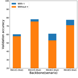
Figure 8: Effect of temperature $\tau$ on MixtFSL using ResNet-12 and -18 in 1- and 5-shot scenarios in miniImageNet’s validation set. The orange bars are the classification results without temperature variable ($\tau=1$), and the blue colored bars are the amount of classification gain by training the backbone with temperature variable ($\tau=0.05$).

We ablate the effect of having a temperature variable $\tau$ in the initial training stage using the validation set. As fig. 8 presents, the validation set accuracy increases with the use of $\tau$ variable across the RN-12 and RN-18. Here, “without $\tau$” corresponds to setting $\tau=1$, and “with $\tau$” to $\tau=0.05$ (found on the validation set).

13 Visualization: from MixtFSL to MixtFSL-Alignment

Fig. 9 summarizes the visualization of embedding space from our mixture-based feature space learning (MixtFSL) to its centroid alignment extension (sec. 6.1 from the main paper). Fig. 9-(a) is a visualization of 200 base examples per class (circles) and the learned class mixture components (diamonds) after the progressive following training stage. Fig. 9-(b) presents the t-SNE visualization of novel class examples (stars) and related base detection (diamonds of the same color) using our proposed MixtFSL. Fig. 9-(c) presents the visualization of fine-tuning the centroid alignment of [1]. Here, the novel examples align to the center of their related bases.

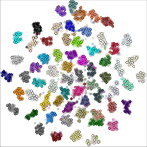
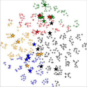
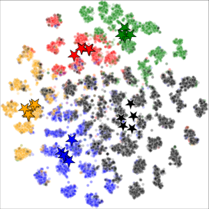
(a) after progressive following	(b) related-modes detection	(c) after alignment

Figure 9: t-SNE [44] applied to the ResNet-12 base feature embedding. (a) learned base categories feature embedding (circles) and mixture components (diamonds) after the progressive following stages. (b) using 5-way (coded by color) novel example shown by stars to detect their related base classes with the learned mixture components shown by diamonds. (b) aligning the novel examples to the center of their related base classes without forgetting the base classes. Points are color-coded by related base and novel examples.

References

- [1] Arman Afrasiyabi, Jean-François Lalonde, and Christian Gagné. Associative alignment for few-shot image classification. In European Conference on Computer Vision, 2020.
- [2] Kelsey R Allen, Evan Shelhamer, Hanul Shin, and Joshua B Tenenbaum. Infinite mixture prototypes for few-shot learning. International Conference on Machine Learning, PMLR, 2019.
- [3] Luca Bertinetto, Joao F. Henriques, Philip Torr, and Andrea Vedaldi. Meta-learning with differentiable closed-form solvers. In International Conference on Learning Representations, 2019.
- [4] Malik Boudiaf, Ziko Imtiaz Masud, Jérôme Rony, José Dolz, Pablo Piantanida, and Ismail Ben Ayed. Transductive information maximization for few-shot learning. Neural Information Processing Systems, 2020.
- [5] Qi Cai, Yingwei Pan, Ting Yao, Chenggang Yan, and Tao Mei. Memory matching networks for one-shot image recognition. In Conference on Computer Vision and Pattern Recognition, 2018.
- [6] Kaidi Cao, Jingwei Ji, Zhangjie Cao, Chien-Yi Chang, and Juan Carlos Niebles. Few-shot video classification via temporal alignment. In International Conference on Computer Vision and Pattern Recognition, 2020.
- [7] Mathilde Caron, Ishan Misra, Julien Mairal, Priya Goyal, Piotr Bojanowski, and Armand Joulin. Unsupervised learning of visual features by contrasting cluster assignments. 2020.
- [8] Wei-Yu Chen, Yen-Cheng Liu, Zsolt Kira, Yu-Chiang Frank Wang, and Jia-Bin Huang. A closer look at few-shot classification. arXiv preprint arXiv:1904.04232, 2019.
- [9] Zitian Chen, Yanwei Fu, Yu-Xiong Wang, Lin Ma, Wei Liu, and Martial Hebert. Image deformation meta-networks for one-shot learning. In International Conference on Computer Vision and Pattern Recognition, 2019.
- [10] Wen-Hsuan Chu, Yu-Jhe Li, Jing-Cheng Chang, and Yu-Chiang Frank Wang. Spot and learn: A maximum-entropy patch sampler for few-shot image classification. In International Conference on Computer Vision and Pattern Recognition, 2019.
- [11] Jiankang Deng, Jia Guo, Niannan Xue, and Stefanos Zafeiriou. Arcface: Additive angular margin loss for deep face recognition. In International Conference on Computer Vision and Pattern Recognition, 2019.
- [12] Guneet S Dhillon, Pratik Chaudhari, Avinash Ravichandran, and Stefano Soatto. A baseline for few-shot image classification. arXiv preprint arXiv:1909.02729, 2019.
- [13] Nikita Dvornik, Cordelia Schmid, and Julien Mairal. Diversity with cooperation: Ensemble methods for few-shot classification. In International Conference on Computer Vision, 2019.
- [14] Qi Fan, Wei Zhuo, Chi-Keung Tang, and Yu-Wing Tai. Few-shot object detection with attention-rpn and multi-relation detector. In International Conference on Computer Vision and Pattern Recognition, 2020.
- [15] Nanyi Fei, Zhiwu Lu, Tao Xiang, and Songfang Huang. Melr: Meta-learning via modeling episode-level relationships for few-shot learning. In International Conference on Learning Representations, 2021.
- [16] Li Fei-Fei, Rob Fergus, and Pietro Perona. One-shot learning of object categories. Transactions on Pattern Analysis and Machine Intelligence, 2006.
- [17] Basura Fernando, Elisa Fromont, Damien Muselet, and Marc Sebban. Supervised learning of gaussian mixture models for visual vocabulary generation. Pattern Recognition, 2012.
- [18] Chelsea Finn, Pieter Abbeel, and Sergey Levine. Model-agnostic meta-learning for fast adaptation of deep networks. In International Conference on Machine Learning, 2017.
- [19] Chelsea Finn, Kelvin Xu, and Sergey Levine. Probabilistic model-agnostic meta-learning. In Neural Information Processing Systems, 2018.
- [20] Hang Gao, Zheng Shou, Alireza Zareian, Hanwang Zhang, and Shih-Fu Chang. Low-shot learning via covariance-preserving adversarial augmentation networks. In Neural Information Processing Systems, 2018.
- [21] Victor Garcia and Joan Bruna. Few-shot learning with graph neural networks. arXiv preprint arXiv:1711.04043, 2017.
- [22] J-L Gauvain and Chin-Hui Lee. Maximum a posteriori estimation for multivariate gaussian mixture observations of markov chains. transactions on speech and audio processing, 1994.
- [23] Spyros Gidaris, Andrei Bursuc, Nikos Komodakis, Patrick Pérez, and Matthieu Cord. Boosting few-shot visual learning with self-supervision. In International Conference on Computer Vision, 2019.
- [24] Spyros Gidaris and Nikos Komodakis. Dynamic few-shot visual learning without forgetting. In International Conference on Computer Vision and Pattern Recognition, 2018.
- [25] Spyros Gidaris and Nikos Komodakis. Generating classification weights with gnn denoising autoencoders for few-shot learning. arXiv preprint arXiv:1905.01102, 2019.
- [26] Xavier Glorot and Yoshua Bengio. Understanding the difficulty of training deep feedforward neural networks. In Thirteenth international conference on artificial intelligence and statistics, 2010.
- [27] Bharath Hariharan and Ross Girshick. Low-shot visual recognition by shrinking and hallucinating features. In International Conference on Computer Vision, 2017.
- [28] Kaiming He, Xiangyu Zhang, Shaoqing Ren, and Jian Sun. Deep residual learning for image recognition. In International Conference on Computer Vision and Pattern Recognition, 2016.
- [29] Nils Lid Hjort, Chris Holmes, Peter Müller, and Stephen G Walker. Bayesian nonparametrics. 2010.
- [30] Ruibing Hou, Hong Chang, Bingpeng MA, Shiguang Shan, and Xilin Chen. Cross attention network for few-shot classification. In Neural Information Processing Systems, 2019.
- [31] Shell Xu Hu, Pablo G Moreno, Yang Xiao, Xi Shen, Guillaume Obozinski, Neil D Lawrence, and Andreas Damianou. Empirical bayes transductive meta-learning with synthetic gradients. International Conference on Learning Representations, 2020.
- [32] Liu Jinlu, Song Liang, and Qin Yongqiang. Prototype rectification for few-shot learning. In European Conference on Computer Vision, 2020.
- [33] Jongmin Kim, Taesup Kim, Sungwoong Kim, and Chang D Yoo. Edge-labeling graph neural network for few-shot learning. In International Conference on Computer Vision and Pattern Recognition, 2019.
- [34] Junsik Kim, Tae-Hyun Oh, Seokju Lee, Fei Pan, and In So Kweon. Variational prototyping-encoder: One-shot learning with prototypical images. In International Conference on Computer Vision and Pattern Recognition, 2019.
- [35] Taesup Kim, Jaesik Yoon, Ousmane Dia, Sungwoong Kim, Yoshua Bengio, and Sungjin Ahn. Bayesian model-agnostic meta-learning. arXiv preprint arXiv:1806.03836, 2018.
- [36] Brian Kulis and Michael I Jordan. Revisiting k-means: New algorithms via bayesian nonparametrics. In International Conference on Machine Learning, 2012.
- [37] Kwonjoon Lee, Subhransu Maji, Avinash Ravichandran, and Stefano Soatto. Meta-learning with differentiable convex optimization. In International Conference on Computer Vision and Pattern Recognition, 2019.
- [38] Junjie Li, Zilei Wang, and Xiaoming Hu. Learning intact features by erasing-inpainting for few-shot classification. In Proceedings of the AAAI Conference on Artificial Intelligence, volume 35, 2021.
- [39] Wenbin Li, Lei Wang, Jinglin Xu, Jing Huo, Yang Gao, and Jiebo Luo. Revisiting local descriptor based image-to-class measure for few-shot learning. In International Conference on Computer Vision and Pattern Recognition, 2019.
- [40] Yann Lifchitz, Yannis Avrithis, Sylvaine Picard, and Andrei Bursuc. Dense classification and implanting for few-shot learning. In International Conference on Computer Vision and Pattern Recognition, 2019.
- [41] Bin Liu, Yue Cao, Yutong Lin, Qi Li, Zheng Zhang, Mingsheng Long, and Han Hu. Negative margin matters: Understanding margin in few-shot classification. In European Conference on Computer Vision, 2020.
- [42] Bin Liu, Zhirong Wu, Han Hu, and Stephen Lin. Deep metric transfer for label propagation with limited annotated data. In International Conference on Computer Vision Workshops, 2019.
- [43] Yanbin Liu, Juho Lee, Minseop Park, Saehoon Kim, Eunho Yang, Sung Ju Hwang, and Yi Yang. Learning to propagate labels: Transductive propagation network for few-shot learning. arXiv preprint arXiv:1805.10002, 2018.
- [44] Laurens van der Maaten and Geoffrey Hinton. Visualizing data using t-sne. Journal of Machine Learning Research, 2008.
- [45] Akshay Mehrotra and Ambedkar Dukkipati. Generative adversarial residual pairwise networks for one shot learning. arXiv preprint arXiv:1703.08033, 2017.
- [46] Nikhil Mishra, Mostafa Rohaninejad, Xi Chen, and Pieter Abbeel. A simple neural attentive meta-learner. arXiv preprint arXiv:1707.03141, 2017.
- [47] Volodymyr Mnih, Koray Kavukcuoglu, David Silver, Andrei A Rusu, Joel Veness, Marc G Bellemare, Alex Graves, Martin Riedmiller, Andreas K Fidjeland, Georg Ostrovski, et al. Human-level control through deep reinforcement learning. nature, 2015.
- [48] Tsendsuren Munkhdalai, Xingdi Yuan, Soroush Mehri, and Adam Trischler. Rapid adaptation with conditionally shifted neurons. In International Conference on Machine Learning, 2018.
- [49] Boris Oreshkin, Pau Rodríguez López, and Alexandre Lacoste. Tadam: Task dependent adaptive metric for improved few-shot learning. In Neural Information Processing Systems, 2018.
- [50] Juan-Manuel Perez-Rua, Xiatian Zhu, Timothy M. Hospedales, and Tao Xiang. Incremental few-shot object detection. In International Conference on Computer Vision and Pattern Recognition, 2020.
- [51] Hang Qi, Matthew Brown, and David G. Lowe. Low-shot learning with imprinted weights. In International Conference on Computer Vision and Pattern Recognition, 2018.
- [52] Limeng Qiao, Yemin Shi, Jia Li, Yaowei Wang, Tiejun Huang, and Yonghong Tian. Transductive episodic-wise adaptive metric for few-shot learning. In IEEE/CVF International Conference on Computer Vision, 2019.
- [53] Siyuan Qiao, Chenxi Liu, Wei Shen, and Alan L. Yuille. Few-shot image recognition by predicting parameters from activations. In International Conference on Computer Vision and Pattern Recognition, 2018.
- [54] Carl Edward Rasmussen. The infinite gaussian mixture model. In Neural Information Processing Systems, 2000.
- [55] Sachin Ravi and Hugo Larochelle. Optimization as a model for few-shot learning. In International Conference on Learning Representations, 2016.
- [56] Ali Razavi, Aaron van den Oord, and Oriol Vinyals. Generating diverse high-fidelity images with vq-vae-2. In Neural Information Processing Systems, 2019.
- [57] Mengye Ren, Eleni Triantafillou, Sachin Ravi, Jake Snell, Kevin Swersky, Joshua B Tenenbaum, Hugo Larochelle, and Richard S Zemel. Meta-learning for semi-supervised few-shot classification. arXiv preprint arXiv:1803.00676, 2018.
- [58] Olga Russakovsky, Jia Deng, Hao Su, Jonathan Krause, Sanjeev Satheesh, Sean Ma, Zhiheng Huang, Andrej Karpathy, Aditya Khosla, Michael Bernstein, et al. Imagenet large scale visual recognition challenge. International Journal of Computer Vision, 2015.
- [59] Andrei A Rusu, Dushyant Rao, Jakub Sygnowski, Oriol Vinyals, Razvan Pascanu, Simon Osindero, and Raia Hadsell. Meta-learning with latent embedding optimization. International Conference on Learning Representations, 2018.
- [60] Eli Schwartz, Leonid Karlinsky, Joseph Shtok, Sivan Harary, Mattias Marder, Abhishek Kumar, Rogerio Feris, Raja Giryes, and Alex Bronstein. Delta-encoder: an effective sample synthesis method for few-shot object recognition. In Neural Information Processing Systems, 2018.
- [61] Zagoruyko Sergey and Komodakis Nikos. Wide residual networks. In British Machine Vision Conference, 2016.
- [62] Christian Simon, Piotr Koniusz, Richard Nock, and Mehrtash Harandi. Adaptive subspaces for few-shot learning. In International Conference on Computer Vision and Pattern Recognition, 2020.
- [63] Christian Simon, Piotr Koniusz, Richard Nock, and Mehrtash Harandi. On modulating the gradient for meta-learning. In European Conference on Computer Vision, 2020.
- [64] Jake Snell, Kevin Swersky, and Richard Zemel. Prototypical networks for few-shot learning. In Neural Information Processing Systems, 2017.
- [65] Jong-Chyi Su, Subhransu Maji, and Bharath Hariharan. When does self-supervision improve few-shot learning? In European Conference on Computer Vision, 2020.
- [66] Qianru Sun, Yaoyao Liu, Tat-Seng Chua, and Bernt Schiele. Meta-transfer learning for few-shot learning. In International Conference on Computer Vision and Pattern Recognition, 2019.
- [67] Flood Sung, Yongxin Yang, Li Zhang, Tao Xiang, Philip H.S. Torr, and Timothy M. Hospedales. Learning to compare: Relation network for few-shot learning. In International Conference on Computer Vision and Pattern Recognition, 2018.
- [68] Kaihua Tang, Jianqiang Huang, and Hanwang Zhang. Long-tailed classification by keeping the good and removing the bad momentum causal effect. Neural Information Processing Systems, 2020.
- [69] Yonglong Tian, Yue Wang, Dilip Krishnan, Joshua B Tenenbaum, and Phillip Isola. Few-shot image classification: a good embedding is all you need. In European Conference on Computer Vision, 2020.
- [70] Hung-Yu Tseng, Hsin-Ying Lee, Jia-Bin Huang, and Ming-Hsuan Yang. Cross-domain few-shot classification via learned feature-wise transformation. arXiv preprint arXiv:2001.08735, 2020.
- [71] Aaron Van Den Oord, Oriol Vinyals, et al. Neural discrete representation learning. In Neural Information Processing Systems, 2017.
- [72] Ricardo Vilalta and Youssef Drissi. A perspective view and survey of meta-learning. Artificial Intelligence Review, 2002.
- [73] Oriol Vinyals, Charles Blundell, Timothy Lillicrap, Daan Wierstra, et al. Matching networks for one shot learning. In Neural Information Processing Systems, 2016.
- [74] Catherine Wah, Steve Branson, Peter Welinder, Pietro Perona, and Serge Belongie. The Caltech-UCSD birds-200-2011 dataset, 2011.
- [75] Yaxing Wang, Salman Khan, Abel Gonzalez-Garcia, Joost van de Weijer, and Fahad Shahbaz Khan. Semi-supervised learning for few-shot image-to-image translation. In International Conference on Computer Vision and Pattern Recognition, 2020.
- [76] Yikai Wang, Chengming Xu, Chen Liu, Li Zhang, and Yanwei Fu. Instance credibility inference for few-shot learning. In International Conference on Computer Vision and Pattern Recognition, 2020.
- [77] Yu-Xiong Wang, Ross Girshick, Martial Hebert, and Bharath Hariharan. Low-shot learning from imaginary data. In International Conference on Computer Vision and Pattern Recognition, 2018.
- [78] Yu-Xiong Wang and Martial Hebert. Learning from small sample sets by combining unsupervised meta-training with cnns. In Neural Information Processing Systems, 2016.
- [79] Yu-Xiong Wang, Deva Ramanan, and Martial Hebert. Meta-learning to detect rare objects. In International Conference on Computer Vision, 2019.
- [80] Davis Wertheimer and Bharath Hariharan. Few-shot learning with localization in realistic settings. In International Conference on Computer Vision and Pattern Recognition, 2019.
- [81] Mike West and Michael D Escobar. Hierarchical priors and mixture models, with application in regression and density estimation. 1993.
- [82] Chengming Xu, Yanwei Fu, Chen Liu, Chengjie Wang, Jilin Li, Feiyue Huang, Li Zhang, and Xiangyang Xue. Learning dynamic alignment via meta-filter for few-shot learning. In Conference on Computer Vision and Pattern Recognition, 2021.
- [83] Sung Whan Yoon, Jun Seo, and Jaekyun Moon. Tapnet: Neural network augmented with task-adaptive projection for few-shot learning. International Conference on Machine Learning, 2019.
- [84] Chi Zhang, Yujun Cai, Guosheng Lin, and Chunhua Shen. Deepemd: Few-shot image classification with differentiable earth mover’s distance and structured classifiers. In International Conference on Computer Vision and Pattern Recognition, 2020.
- [85] Hongyi Zhang, Moustapha Cisse, Yann N Dauphin, and David Lopez-Paz. mixup: Beyond empirical risk minimization. arXiv preprint arXiv:1710.09412, 2017.
- [86] Hongguang Zhang, Jing Zhang, and Piotr Koniusz. Few-shot learning via saliency-guided hallucination of samples. In International Conference on Computer Vision and Pattern Recognition, 2019.
- [87] Jian Zhang, Chenglong Zhao, Bingbing Ni, Minghao Xu, and Xiaokang Yang. Variational few-shot learning. In International Conference on Computer Vision, 2019.
- [88] Manli Zhang, Jianhong Zhang, Zhiwu Lu, Tao Xiang, Mingyu Ding, and Songfang Huang. Iept: Instance-level and episode-level pretext tasks for few-shot learning. In International Conference on Learning Representations, 2021.
- [89] Jiabao Zhao, Yifan Yang, Xin Lin, Jing Yang, and Liang He. Looking wider for better adaptive representation in few-shot learning. In Proceedings of the AAAI Conference on Artificial Intelligence, 2021.
- [90] Imtiaz Ziko, Jose Dolz, Eric Granger, and Ismail Ben Ayed. Laplacian regularized few-shot learning. In International Conference on Machine Learning, 2020.