Geometrical dependence in Casimir-Polder repulsion: Anisotropically polarizable atom and anisotropically polarizable annular dielectric

Abstract

Casimir-Polder interaction energies between a point anisotropically polarizable atom and an annular dielectric are shown to exhibit localized repulsive long-range forces in specific configurations. We show that when the atom is positioned at the center of the annular dielectric, it is energetically favorable for the atom to align its polarizability with respect to that of the dielectric. As the atom moves away from, but along the symmetry axis of the annular dielectric, it encounters a point where the polarizable atom experiences no torque and the energy is free of orientation dependence. At this height, abruptly, the atom prefers to orient its polarizability perpendicular to that of the dielectric. For certain configurations, it encounters another torsion-free point a larger distance away, beyond which it prefers to again point its polarizability with respect to that of the dielectric. We find when the atom is close enough, and oriented such that the energy is close to maximum, the atom could be repelled. For certain annular polarizations, repulsion can happen below or above the torsion-free height. Qualitative features differ when the atom is interacting with a ring, versus a plate of infinite extent with a hole. In particular, the atom can prefer to orient perpendicular to the polarizability of the plate at large distances, in striking contrast to the expectation that it will orient parallel. To gain insight of this discrepancy, we investigate an annular disc, which captures the results of both geometries in limiting cases. These energies are too weak for immediate applications, nevertheless, we elaborate an interesting application on a prototype of a Casimir machine using these configurations.

I Introduction

The term Casimir effect has come to refer to the entire phenomena associated with quantum fluctuations in electrodynamics. Figure 1 shows a schematic diagram that identifies the various domains in interactions mediated by quantum fluctuations. The van der Waals van der Waals (1873) and London dispersion forces Eisenschitz and London (1930); London (1930); Hettema (2000) govern these interactions in the non-retarded weak regime, while the Casimir-Polder interaction energy Casimir and Polder (1948) involves interactions between weak dielectric materials in the retarded regime. The energies in the weak regime are often easier to compute. In contrast, the Casimir energy between highly conducting materials in the retarded regime are typically hard to compute because it involves identification and subtraction of divergences in non-trivial ways to arrive at the expression for energy. The Casimir energy is also very sought-after because it is a manifestation of zero point energy associated to the quantum vacuum Casimir (1948); Milton (2011). The limiting forms in Fig. 1 are generalized by the Lifshitz formula Lifshitz (1956), and were further generalized and studied by Dzyaloshinskii, Lifshitz, and Pitaevskii (DLP) Dzyaloshinskii et al. (1961).

The Casimir effect most often leads to attractive forces between objects, and the plausibility of associated repulsive forces has always captivated attention. In the non-retarded van der Waals regime of Fig. 1, repulsion has been predicted in three-body interactions at least since the work of Axilrod and Teller Axilrod and Teller (1943) and Muto Muto (1943). In the Casimir-Polder regime, repulsion between anisotropically polarizable atoms was predicted in the works of Craig and Power Craig and Power (1969a, b) and has been extensively explored since then; see Ref. Babb (2005) and references therein. However, it was not until a decade ago when it was realized that similar repulsive behavior was plausible in the Casimir regime of Fig. 1. This came by in Ref. Levin et al. (2010), where it was argued on physical grounds that the interaction energy between an elongated needle-shaped-conductor and a perfectly conducting metal sheet with a circular aperture could have a local minima. They showed that the Casimir force could become repulsive when the needle got sufficiently close to the aperture. This also meant that the force between a charge placed in front a perfectly conducting object could be repulsive Levin and Johnson (2011), and similar configurations were further explored in Ref. McCauley et al. (2011). It was realized there that the anisotropy in the geometry of a highly conducting object corresponds to an effective anisotropic permittivity and the interplay of these anisotropic permittivities leads to non-monotonic interaction energies that show repulsion. These remarkable predictions were based on symmetry arguments and were confirmed using numerical calculations.

Here we list some of the attempts made towards understanding the result in Ref. Levin et al. (2010) analytically. In Ref.Eberlein and Zietal (2011), it was shown that even in the non-retarded van der Waals regime, similar configurations lead to repulsion. They used the method of inversion that was successfully used in the heyday of electrostatics. In Ref. Abrantes et al. (2018), the method of inversion was again used to show that in the non-retarded van der Waals regime an anisotropically polarizable atom placed along the symmetry axis of a toroid could experience repulsion. In Refs. Shajesh and Schaden (2012) and Milton et al. (2012a), it was shown that in the retarded Casimir-Polder regime of Fig. 1, repulsion is possible in configurations with anisotropically polarizable atoms and anisotropic dielectric materials. An analytic formula for the Casimir-Polder energy between dielectric bodies was derived in Refs. Shajesh and Schaden (2012) and Milton et al. (2012a). In particular, a closed form expression for the force between an anisotropically polarizable atom and a dielectric plate with a circular aperture was shown to demonstrate repulsion. In spite of the above successes in the weak scenario, and having numerically found configurations exhibiting repulsion in the Casimir regime of Fig. 1, analytic derivation of a closed-form expression for the interaction energy between a polarizable atom and a highly conducting plate with an aperture still remains an open problem. Initiative towards such a derivation has been presented in Refs. Milton et al. (2011) and Milton et al. (2012b). Another proposal was to exploit the axial symmetry of the configuration Shajesh et al. (2017). However, a closed-form analytic result remains elusive.

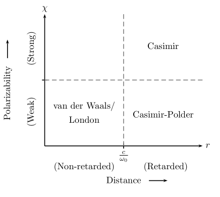
Figure 1: Diagram showing terminology associated with interactions mediated by quantum fluctuations in electrodynamics. Here $\chi$ is the dielectric susceptibility of a material characterized by plasma frequency $\omega_{p}$, $\omega_{0}$ is a characteristic frequency of the material, $c$ is speed of light in vacuum, and $r$ is the distance between two objects.

In this paper we investigate the interaction energy between two neutral anisotropically polarizable objects mediated by quantum fluctuations. We ignore magnetization effects here. The outline of the paper and summary of results are as follows: In Sec. II, we derive the interaction energy between a point permanent dipole and an electrically polarized ring. We give a summary of the formalism in Sec. III, and present a few more configurations related to annular plate in Sec. IV. We take up the study of a point anisotropically polarizable atom and an anisotropically polarizable dielectric ring using methods of Ref. Shajesh and Schaden (2012) in Sec. V. We show that for specific orientations of the polarizability, the atom experiences a repulsive force when the atom is very close to the ring. We analyze the orientation dependence and distance dependence of the interaction energies. We also observe that for specific orientations the atom experiences a second repulsive region along the symmetry axis, which is a new finding here. In Sec. VI, we derive the interaction energy between an atom and a dielectric annular disc. For large outer radius, this energy approaches the interaction energy between an atom and a plate with circular aperture. When the outer radius and inner radius of the annular disc are close to each other, the energy approaches that of a ring. In Sec. VII, we highlight and summarize our results. We point out that there exists two torsion free points on each side of the annular disc, where the interaction energy is orientation independent. The position of these points vary with geometric changes to the disk, and differently according to the polarizability; determining large distance orientation dependence. In the ring limit of the annular disc, new repulsion emerges. A brief summary of our results here has been separately presented in Ref. Marchetta et al. (2020), and the exposition here serves as supplementary material for the article. In Sec. VIII, we describe an application of these results in the construction of a Casimir machine. We give concluding remarks in Sec. IX.

For completeness, we list two other classes of repulsive behaviors that are possible between neutral polarizable objects. One of these was mentioned in Ref. Dzyaloshinskii et al. (1961) in which repulsion is possible whenever the dielectric strength of the intervening medium is stronger relative to the surrounding media. The second is associated to repulsion arising from an interplay of electric and magnetic properties of the neutral objects Feinberg and Sucher (1968). In the current level of our understanding, apparently, these repulsions have different origins from those discussed in this paper. The repulsion studied in this article is geometric in origin due to the presumable direct relationship between the effective anisotropies in the dielectric susceptibility and the respective anisotropies in the geometric shape of the conductor. The repulsive nature of self interaction of a single conducting sphere Boyer (1968) could also probably be related to this geometric origin, however it is not an interaction energy between two objects as it is for cases we are considering here.

II Electrostatic analog: Point electric dipole above an electrically polarized ring

Let us begin with an example involving neutral objects having permanent electric polarizations. It will be a prelude for the following discussion involving only neutral induced dipoles.

A point (permanent) electric dipole ${\bf p}$ at position ${\bf r}_{0}$ is suitably described by the charge density

$$\rho_{1}({\bf x})=-{\bf p}\cdot{\bm{\nabla}}\delta^{(3)}({\bf x}-{\bf r}_{0}),$$ (1)

and a (permanent) electrically polarized ring of radius $a$ with dipole per unit length or polarization ${\bm{\lambda}}$ is described by the charge density

$$\rho_{2}({\bf x}^{\prime})=-{\bm{\lambda}}\cdot{\bm{\nabla}}^{\prime}\delta(z^{\prime}-z_{a})\delta(\rho^{\prime}-a),$$ (2)

such that the plane of the ring is perpendicular to the $z$ axis at $z^{\prime}=z_{a}$ with center of the ring on the $z$ axis, see inset in Fig. 2. The electrostatic interaction energy between the point dipole and the ring, in SI units, is given by

$$E_{12}=\frac{1}{4\pi\varepsilon_{0}}\int d^{3}x\int d^{3}x^{\prime}\frac{\rho_{1}({\bf x})\rho_{2}({\bf x}^{\prime})}{|{\bf x}-{\bf x}^{\prime}|}.$$ (3)

Five of the six integrals are immediately completed using the property of $\delta$-functions appearing in the charge densities in Eqs. (1) and (2). This leads to the interaction energy between the point dipole and the ring

$$E_{12}=\frac{1}{4\pi\varepsilon_{0}}\int_{0}^{2\pi}ad\phi^{\prime}\frac{\left[({\bf p}\cdot{\bm{\lambda}})-3({\bf p}\cdot\hat{\bf r})(\hat{\bf r}\cdot{\bm{\lambda}})\right]}{r^{3}},$$ (4)

where we have set

$${\bf r}={\bf x}-{\bf x}^{\prime}.$$ (5)

The magnitude of ${\bf r}$ is $r$ and the unit vector $\hat{\bf r}={\bf r}/r$. Here ${\bf r}$ is the position of the electric dipole relative to the position of a line element $ad\phi^{\prime}$ on the ring that can be explicitly expressed using

$${\bf x} = \rho\cos\phi\,\hat{\bf x}+\rho\sin\phi\,\hat{\bf y}+(z_{a}+h)\,\hat{\bf z},$$ (6a)

$${\bf x}^{\prime} = a\cos\phi^{\prime}\,\hat{\bf x}+a\sin\phi^{\prime}\,\hat{\bf y}+z_{a}\,\hat{\bf z},$$ (6b)

${\bf r}_{0}={\bf x}$, such that

$$r^{2}=a^{2}+h^{2}+\rho^{2}-2a\rho\cos(\phi-\phi^{\prime}).$$ (7)

For the particular case when the ring is polarized in the tangential direction $\hat{\bm{\phi}}^{\prime}$,

$${\bm{\lambda}}=\lambda\hat{\bm{\phi}}^{\prime},$$ (8)

and the position of the point dipole is confined on the symmetry axis of the ring, $\rho=0$, the interaction energy is

$$E_{12}=0$$ (9)

irrespective of the direction of its dipole moment ${\bf p}$. This is so because $(\hat{\bf r}\cdot{\bm{\lambda}})=\lambda(\hat{\bf r}\cdot\hat{\bm{\phi}}^{\prime})=0$ and the integration

$$\int_{0}^{2\pi}d\phi^{\prime}\,({\bf p}\cdot{\bm{\lambda}})=0$$ (10)

in this case, which involves integration of a cosine function over its complete period.

For the case when the polarization of the ring is aligned to its symmetry axis, and the electric dipole ${\bf p}$ is positioned on the axis and the direction of ${\bf p}$ makes an angle $\theta$ with respect to the symmetry axis,

$${\bm{\lambda}}=\lambda\,\hat{\bf z},\qquad\hat{\bm{\lambda}}\cdot\hat{\bf p}=\cos\theta,\qquad\rho=0.$$ (11)

The interaction energy in this case is

$$E_{12}=\frac{{\bf p}\cdot{\bm{\lambda}}}{a^{2}}\frac{2\pi}{4\pi\varepsilon_{0}}\frac{a^{3}(a^{2}-2h^{2})}{\left(a^{2}+h^{2}\right)^{\frac{5}{2}}}.$$ (12)

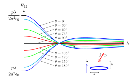
Figure 2: Electrostatic interaction energy between a point electric dipole ${\bf p}$ and a polarized ring of polarization ${\bm{\lambda}}$ as given by Eq. (12). Here $E_{12}$ is plotted with respect to $h$ for $\theta=0^{\circ},30^{\circ},60^{\circ},75^{\circ}$. The energy at $\theta=0$ and $h=0$ is $p\lambda 2\pi/a^{2}4\pi\varepsilon_{0}$.

The force in the $z$-direction, a manifestation of change in energy with respect to $h$, is

$${\bf F}\cdot\hat{\bf z}=-\frac{\partial E_{12}}{\partial h}=\frac{{\bf p}\cdot{\bm{\lambda}}}{a^{3}}\frac{2\pi}{4\pi\varepsilon_{0}}\frac{3a^{4}h(3a^{2}-2h^{2})}{\left(a^{2}+h^{2}\right)^{\frac{7}{2}}}$$ (13)

and the torque, a manifestation of change in energy with respect $\theta$, is

$${\bm{\tau}}=-\frac{\partial E_{12}}{\partial\theta}=\frac{{\bf p}\times{\bm{\lambda}}}{a^{2}}\frac{2\pi}{4\pi\varepsilon_{0}}\frac{a^{3}(a^{2}-2h^{2})}{\left(a^{2}+h^{2}\right)^{\frac{5}{2}}}.$$ (14)

The interaction energy of Eq. (12) is plotted as a function of $h$ for different values of orientation angle $\theta$ in Fig. 2. The polarizations of the dipole and the ring prefer to align anti-parallelly for $h\ll a$ and parallelly for $h\gg a$. The energy is zero and torsion-free when $h=a/\sqrt{2}$, represented by the point where all the curves intersect in Fig. 2.

III Formalism

.

We now turn our attention to the interaction between neutral polarizable objects. As mentioned in Introduction, the interaction energy between polarizable materials is governed by the van der Waals and London interaction van der Waals (1873); Eisenschitz and London (1930); London (1930), which generalizes to the Casimir and the Lifshitz interaction Casimir (1948); Lifshitz (1956); Dzyaloshinskii et al. (1961) when retardation effects are taken into account. In the following, we illustrate the formalism. This section is pedagogical and aimed towards listing various approximations in the discussion.

The Casimir or Lifshitz interaction energy between two dielectric materials can be expressed as Shajesh and Schaden (2011)

$$E_{12}=\frac{\hbar c}{2}\int_{-\infty}^{\infty}\frac{d\zeta}{2\pi}\,\text{Tr}\ln\Big{[}{\bf 1}-{\bf\Gamma}_{0}\cdot{\bf T}_{1}\cdot{\bf\Gamma}_{0}\cdot{\bf T}_{2}\Big{]}$$ (15)

in the multiple scattering formalism, where $i\zeta=\omega/c$ is the imaginary frequency and $\omega$ is the frequency. The free Green’s dyadic ${\bf\Gamma}_{0}$ in Eq. (15) satisfies the dyadic differential equation

$$-\Big{[}\frac{1}{\zeta^{2}}{\bm{\nabla}}\times({\bm{\nabla}}\times{\bf 1})+{\bf 1}\Big{]}\cdot{\bm{\Gamma}}_{0}({\bf r};i\zeta)={\bf 1}\,\delta^{(3)}({\bf r})$$ (16)

with solution

$${\bf\Gamma}_{0}({\bf r};i\zeta)=\frac{e^{-|\zeta|r}}{4\pi\,r^{3}}\Big{[}-u(|\zeta|r)\,{\bf 1}+v(|\zeta|r)\,\hat{\bf r}\hat{\bf r}\Big{]},$$ (17)

where

$$u(x) = 1+x+x^{2},$$ (18a)

$$v(x) = 3+3x+x^{2}.$$ (18b)

The electric susceptibilities of the dielectric materials, of electric permittivity ${\bm{\varepsilon}}_{i}$, is

$${\bm{\chi}}_{i}({\bf x};i\zeta)=\frac{{\bm{\varepsilon}}_{i}({\bf x};i\zeta)}{\varepsilon_{0}}-{\bf 1},$$ (19)

where $i=1,2$, denotes respective material. In terms of electric susceptibilities the transition matrices ${\bf T}_{i}$’s in Eq. (15) are symbolically defined by the relation

$${\bf T}_{i}={\bm{\chi}}_{i}\cdot\big{[}{\bf 1}-{\bm{\Gamma}}_{0}\cdot{\bm{\chi}}_{i}\big{]}^{-1}.$$ (20)

The transition matrices are themselves local quantities, but for mathematical purposes are represented as a kernel,

$${\bf T}_{i}({\bf x},{\bf x}^{\prime};i\zeta)={\bf T}_{i}({\bf x};i\zeta)\,\delta^{(3)}({\bf x}-{\bf x}^{\prime}).$$ (21)

The transition matrices are determined by solving the Green’s dyadic equation

$$-\Big{[}\frac{1}{\zeta^{2}}{\bm{\nabla}}\times({\bm{\nabla}}\times{\bf 1})+{\bf 1}+{\bm{\chi}}({\bf x};i\zeta)\Big{]}\cdot{\bm{\Gamma}}_{i}({\bf x},{\bf x}^{\prime};i\zeta)={\bf 1}\,\delta^{(3)}({\bf x}-{\bf x}^{\prime}),$$ (22)

where ${\bm{\Gamma}}_{i}({\bf x},{\bf x}^{\prime};i\zeta)$ are the Green’s dyadic for the individual materials

$${\bm{\Gamma}}_{i}={\bm{\Gamma}}_{0}-{\bm{\Gamma}}_{0}\cdot{\bf T}_{i}\cdot{\bm{\Gamma}}_{0}.$$ (23)

III.1 Point atom

Neglecting quadruple and higher moments, the scattering matrix ${\bf T}_{\text{atom}}$ for an atom with atomic dipole polarizability ${\bm{\alpha}}(i\zeta)$ will be modeled as

$${\bf T}_{\text{atom}}({\bf x};i\zeta)=4\pi{\bm{\alpha}}(i\zeta)\,\delta^{(3)}({\bf x}-{\bf x}_{0}),$$ (24)

where ${\bf x}_{0}$ specifies the position of the atom. The polarizabilities are frequency dependent. The $\delta$-functions in Eq. (24) permit a trivial evaluation of half of the spatial integrals in the trace of Eq. (15). The frequency dependence of the atomic polarizability ${\bm{\alpha}}(i\zeta)$ is in general very complicated and depends on the energy levels of the individual atom. For example, if one assumes a two-level atom with a spherically symmetric ground state and a spherically asymmetric excited state, then a simple model for the frequency dependence of the atomic polarizability is

$${\bm{\alpha}}(i\zeta)={\bm{\alpha}}(0)\frac{\omega_{0}^{2}}{\omega_{0}^{2}+\zeta^{2}c^{2}},$$ (25)

where $\omega_{0}$ is the excitation energy of the (two-level) atom and ${\bm{\alpha}}(0)$ is its static polarizability and a measure of the spherical asymmetry of the excited state. In terms of the radius $a_{0}$ of this simple (two-level) atom, the atomic polarizability could be further modeled as

$${\bm{\alpha}}(0)=\tilde{\bm{\alpha}}_{0}\,a_{0}^{3}.$$ (26)

In this manner, one captures the content of the spherical asymmetry in the excited state in the dimensionless parameter $\tilde{\bm{\alpha}}_{0}$. Formally, we are ignoring the detailed structure of the transition matrix for an atom by replacing Eq. (20) in place with Eq. (24), and is valid for separation distances satisfying

$$|\tilde{\bm{\alpha}}_{0}|\,a_{0}\ll r,$$ (27)

because the propagators inside Eq. (20) rarely span distances greater than the atomic size. This approximation is valid for dilute polarizability, $|\tilde{\bm{\alpha}}_{0}|\ll 1$, and atomic size small compared to separation distance. In this atomic approximation one needs to retain only the leading term of the logarithm after expansion of Eq. (15),

$$E_{\text{atom}}^{\text{W}}({\bm{\alpha}},{\bm{\chi}};{\bf x}_{0})=-\hbar c\int_{-\infty}^{\infty}d\zeta\int d^{3}x\,\hskip 71.13188pt$$

$$\,\text{tr}\,{\bm{\alpha}}(i\zeta)\cdot{\bm{\Gamma}}({\bf x}_{0}-{\bf x};i\zeta)\cdot{\bf T}({\bf x};i\zeta)\cdot{\bm{\Gamma}}_{0}({\bf x}-{\bf x}_{0};i\zeta),\hskip 14.22636pt$$ (28)

where the trace, tr, is over the dyadic index, and ${\bf T}$ is the transition matrix of the dielectric material that the atom is interacting with. Substituting the free Green’s dyadic from Eq. (17) into Eq. (28) we have

$$E_{\text{atom}}^{\text{W}}({\bm{\alpha}},{\bm{\chi}};{\bf x}_{0})=-\frac{\hbar c}{16\pi^{2}}\int_{-\infty}^{\infty}d\zeta\int d^{3}x\,\frac{e^{-2|\zeta|r}}{r^{6}}\hskip 28.45274pt$$

$$\hskip 28.45274pt\times\Big{[}u^{2}(\zeta r)\,\text{tr}\{{\bm{\alpha}}(i\zeta)\cdot{\bf T}({\bf x};i\zeta)\}$$

$$\hskip 39.83385pt-2u(\zeta r)v(\zeta r)\,\{\hat{\bf r}\cdot{\bm{\alpha}}(i\zeta)\cdot{\bf T}({\bf x};i\zeta)\cdot\hat{\bf r}\}$$

$$\hskip 39.83385pt+v^{2}(\zeta r)\,\{\hat{\bf r}\cdot{\bm{\alpha}}(i\zeta)\cdot\hat{\bf r}\}\{\hat{\bf r}\cdot{\bf T}({\bf x};i\zeta)\cdot\hat{\bf r}\}\Big{]},$$ (29)

where ${\bf r}={\bf x}-{\bf x}_{0}$, and $r=|{\bf r}|$. We used the property that atomic polarizability ${\bm{\alpha}}$ and the transition matrix ${\bf T}$ are symmetric tensors that let us combine the two cross terms into a single one.

III.2 van der Waals-London approximation

The non-retarded (van der Waals-London) regime,

$$|{\bm{\alpha}}(0)|^{1/3}<r\ll\frac{c}{\omega_{0}},$$ (30)

is a short-range approximation, where short is in relation to the characteristic length associated with resonant frequency. In the regime of Eq. (30), the frequency dependence in Eq. (17) may be neglected and the free dyadic in Eq. (28) is approximated by the static dipole-dipole interaction ${\bm{\Gamma}}_{0}({\bm{r}};0)$ to yield Craig and Power (1969a, b), using Eq. (28),

$$E_{\text{atom}}^{\text{Lon}}({\bm{\alpha}},{\bm{\chi}};{\bf x}_{0})=\hbar c\int_{-\infty}^{\infty}d\zeta\int d^{3}x\hskip 71.13188pt$$

$$\hskip 11.38109pt\,\text{tr}\,{\bm{\alpha}}(i\zeta)\cdot{\bm{\Gamma}}({\bf x}_{0}-{\bf x};0)\cdot{\bf T}({\bf x};i\zeta)\cdot{\bm{\Gamma}}({\bf x}-{\bf x}_{0};0).$$ (31)

In this the way, Eq. (29) simplifies to

$$E_{\text{atom}}^{\text{Lon}}({\bm{\alpha}},{\bm{\chi}};{\bf x}_{0})=-\frac{\hbar c}{16\pi^{2}}\int_{-\infty}^{\infty}d\zeta\int d^{3}x\,\frac{1}{r^{6}}$$

$$\hskip 28.45274pt\times\Big{[}\,\text{tr}\{{\bm{\alpha}}(i\zeta)\cdot{\bf T}({\bf x};i\zeta)\}-6\,\{\hat{\bf r}\cdot{\bm{\alpha}}(i\zeta)\cdot{\bf T}({\bf x};i\zeta)\cdot\hat{\bf r}\}$$

$$\hskip 39.83385pt+9\,\{\hat{\bf r}\cdot{\bm{\alpha}}(i\zeta)\cdot\hat{\bf r}\}\{\hat{\bf r}\cdot{\bf T}({\bf x};i\zeta)\cdot\hat{\bf r}\}\Big{]},$$ (32)

which uses $u(0)=1$ and $v(0)=3$. For two atoms with isotropic polarizabilities, this reproduces London’s expression for the van der Waals interaction

$$E_{\text{atom-atom}}^{\text{Lon}}(\alpha_{1}{\bf 1},\alpha_{2}{\bf 1};r)=-\frac{3\hbar c}{\pi\,r^{6}}\int_{0}^{\infty}d\zeta\,\alpha_{1}(i\zeta)\alpha_{2}(i\zeta),$$ (33)

which is inversely proportional to the sixth power in the separation $r$.

III.3 Casimir-Polder approximation

The retarded (Casimir-Polder) regime,

$$|{\bm{\alpha}}(0)|^{1/3}<\frac{c}{\omega_{0}}\ll r,$$ (34)

is the corresponding long-range approximation when only fluctuations of very large time period (small frequency) contribute to resonance. In this approximation, the exponential dependence on the separation distance in the free propagator of Eq. (17) implies that the frequency dependence of the polarizability ${\bm{\alpha}_{i}}(i\zeta)$ in Eq. (25) is negligible. In the Casimir-Polder regime, the polarizabilities can be approximated by their static values in Eq. (28) to yield Craig and Power (1969a, b),

$$E_{\text{atom}}^{\text{CP}}({\bm{\alpha}},{\bm{\chi}};{\bf x}_{0})=-\hbar c\int_{-\infty}^{\infty}d\zeta\int d^{3}x\,\hskip 56.9055pt$$

$$\hskip 14.22636pt\times\,\text{tr}\,{\bm{\alpha}}(0)\cdot{\bm{\Gamma}}({\bf x}_{0}-{\bf x};i\zeta)\cdot{\bf T}({\bf x};0)\cdot{\bm{\Gamma}}({\bf x}-{\bf x}_{0};i\zeta).\hskip 14.22636pt$$ (35)

The $\zeta$-integration in Eq. (29) can be performed in this approximation to obtain

$$E_{\text{atom}}^{\text{CP}}({\bm{\alpha}},{\bm{\chi}};{\bf x}_{0})=-\frac{\hbar c}{32\pi^{2}}\int d^{3}x\,\frac{1}{r^{7}}$$

$$\hskip 14.22636pt\times\Big{[}13\,\text{tr}\{{\bm{\alpha}}(0)\cdot{\bf T}({\bf x};0)\}-56\,\{\hat{\bf r}\cdot{\bm{\alpha}}(0)\cdot{\bf T}({\bf x};0)\cdot\hat{\bf r}\}$$

$$\hskip 25.60747pt+63\,\{\hat{\bf r}\cdot{\bm{\alpha}}(0)\cdot\hat{\bf r}\}\{\hat{\bf r}\cdot{\bf T}({\bf x};0)\cdot\hat{\bf r}\}\Big{]}.$$ (36)

For atoms with isotropic polarizabilities ${\bm{\alpha}}_{1}=\alpha_{1}{\bf 1}$ and ${\bm{\alpha}}_{2}=\alpha_{2}{\bf 1}$, Eq. (36) reproduces the Casimir-Polder interaction Casimir and Polder (1948)

$$E_{12}^{\text{CP}}(\alpha_{1}{\bf 1},\alpha_{2}{\bf 1};r)=-\frac{23\hbar c}{4\pi}\frac{\alpha_{1}(0)\alpha_{2}(0)}{r^{7}},$$ (37)

which is inversely proportional to the seventh power in the separation $r$.

III.4 Dilute dielectric approximation

For a dilute dielectric material, we have

$${\bm{\chi}}\ll{\bf 1}.$$ (38)

Thus, after keeping the leading term in the expansion of Eq. (20), the scattering matrix for the dilute material becomes

$${\bf T}_{i}({\bf x},{\bf x}^{\prime};i\zeta)\sim{\bm{\chi}}_{i}({\bf x};i\zeta)\,\delta^{(3)}({\bf x}-{\bf x}^{\prime}).$$ (39)

The dilute dielectric approximation of Eq. (28) is

$$E_{\text{atom-dd}}^{\text{W}}=-\hbar c\int_{-\infty}^{\infty}d\zeta\int d^{3}x$$

$$\hskip 8.53581pt\,\text{tr}\,{\bm{\alpha}}(i\zeta)\cdot{\bm{\Gamma}}_{0}({\bf x}_{0}-{\bf x};i\zeta)\cdot{\bm{\chi}}({\bf x};i\zeta)\cdot{\bm{\Gamma}}_{0}({\bf x}-{\bf x}_{0};i\zeta).\hskip 19.91692pt$$ (40)

The London interaction energies in Eqs. (31) and (32), and the Casimir-Polder energies in Eqs. (35) and (36), in the approximation of Eq. (38) are immediately obtained by the replacement: ${\bf T}\to{\bm{\chi}}$. For example, the Casimir-Polder interaction energy between an atom and a dilute dielectric, using Eq. (24) and Eq. (19), is given by

$$E_{\text{atom-dd}}^{\text{CP}}({\bm{\alpha}},{\bm{\chi}};{\bf x}_{0})=-\frac{\hbar c}{32\pi^{2}}\int d^{3}x\,\frac{1}{r^{7}}$$

$$\hskip 14.22636pt\times\Big{[}13\,\text{tr}\{{\bm{\alpha}}(0)\cdot{\bm{\chi}}({\bf x};0)\}-56\,\{\hat{\bf r}\cdot{\bm{\alpha}}(0)\cdot{\bm{\chi}}({\bf x};0)\cdot\hat{\bf r}\}$$

$$\hskip 25.60747pt+63\,\{\hat{\bf r}\cdot{\bm{\alpha}}(0)\cdot\hat{\bf r}\}\{\hat{\bf r}\cdot{\bm{\chi}}({\bf x};0)\cdot\hat{\bf r}\}\Big{]},$$ (41)

which is a ready-to-use expression, because unlike the earlier approximations, it does not require the solution for the transition matrix ${\bf T}$ obtained by solving the Green’s dyadic equation in Eq. (22). The dilute-dielectric approximation seems to always contain all the qualitative features of the interaction energy, and thus serves well for a qualitative understanding of complicated geometries.

IV Point atom above an infinite dielectric plate with a circular aperture

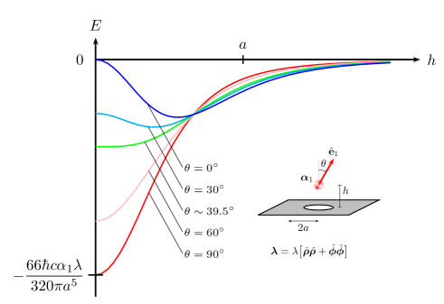
Figure 3: The energy of Eq. (45) is plotted as a function of height $h$ for an anisotropic atom above the center of a dielectric plate with an aperture of radius $a$ as sketched in the insert. The curves correspond to different orientation $\theta$ of the atomic polarizability.

As a demonstration of the use of Eq. (41), in Ref. Shajesh and Schaden (2012), the energy expression of Eq. (41) was used to determine the interaction energy of an atom with polarizability,

$${\bm{\alpha}}=\alpha_{1}\,\hat{\bf e}_{1}\,\hat{\bf e}_{1},\quad\hat{\bf e}_{1}\cdot\hat{\bf z}=\cos\theta,$$ (42)

with a dielectric plate of infinite extent with a circular aperture of radius $a$ with polarizability

$${\bm{\chi}}={\bm{\lambda}}\,\theta(\sqrt{x^{2}+y^{2}}-a)\,\delta(z)$$ (43)

when the atom is positioned on the symmetry axis of the plate.

IV.1 Partially isotropic plate

For the case when dilute dielectric plate has isotropic polarizability in the plane of the plate we have

$${\bm{\lambda}}=\lambda\big{[}\hat{\bf x}\hat{\bf x}+\hat{\bf y}\hat{\bf y}\big{]}=\lambda\big{[}\hat{\bm{\rho}}\hat{\bm{\rho}}+\hat{\bm{\phi}}\hat{\bm{\phi}}\big{]}.$$ (44)

The interaction energy has the closed form exact expression

$$E = -\frac{\hbar c\alpha_{1}\lambda}{64\pi}\frac{1}{5}\frac{1}{(a^{2}+h^{2})^{\frac{9}{2}}}\Big{[}(33a^{4}+106a^{2}h^{2}+38h^{4})$$ (45)

$$\hskip 28.45274pt-(33a^{4}-74a^{2}h^{2}-2h^{4})\cos 2\theta\Big{]}.\hskip 17.07164pt$$

Fig. 3 shows the dependence of Eq. (45) on the height $h$ for different orientations $\theta$ of the anisotropic atom. The parameter space of height $h$ and orientation angle $\theta$ that leads to repulsion has been shown as shaded regions in Fig. 4. Repulsion ceases for orientations $\theta>\cos^{-1}(17/89)/2\sim 39.49^{\circ}$. We refer to Ref. Shajesh and Schaden (2012) for a detailed discussion. We point out that the expression for interaction energy in Eq. (18) in Ref. Shajesh and Schaden (2012) has errors in the coefficients there and should be replaced with the correct form in Eq. (45). This error propagates into the analysis of repulsion there, however, all the qualitative features of the result and associated conclusions remain unchanged.

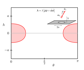
Figure 4: The shaded regions in the parameter space of height $h$ and orientation angle $\theta$ above leads to repulsion between an anisotropic atom at a height $h$ above the center of a dielectric plate with an aperture of radius $a$ as sketched in the insert.

IV.2 Radially polarizable plate with aperture

When the dilute dielectric plate is polarizable in the radial directions, we have

$${\bm{\lambda}}=\lambda_{\rho}\hat{\bm{\rho}}\hat{\bm{\rho}}.$$ (46)

The interaction energy has the form

$$E = -\frac{\hbar c\alpha_{1}\lambda_{\rho}}{64\pi}\frac{1}{(a^{2}+h^{2})^{\frac{9}{2}}}\Big{[}(4a^{4}+16a^{2}h^{2}+5h^{4})$$ (47)

$$\hskip 28.45274pt-(4a^{4}-20a^{2}h^{2}-3h^{4})\cos 2\theta\Big{]}.\hskip 17.07164pt$$

The qualitative features of energy plots is completely captured in the corresponding energy plots for the partially isotropic case in Fig. 4. We shall return to the expression for energy in Eq. (47) while discussing the case of a circular disc with circular aperture as the outer radius of the disc extends to infinity.

IV.3 Axially polarizable plate with aperture

When the dilute dielectric plate is polarizable in the direction of its symmetry axis, we have

$${\bm{\lambda}}=\lambda_{z}\hat{\bf z}\hat{\bf z}.$$ (48)

The interaction energy has the form

$$E = -\frac{\hbar c\alpha_{1}\lambda_{z}}{64\pi}\frac{1}{5}\frac{1}{(a^{2}+h^{2})^{\frac{9}{2}}}\Big{[}(26a^{4}+17a^{2}h^{2}+26h^{4})$$ (49)

$$\hskip 28.45274pt+(26a^{4}-73a^{2}h^{2}+6h^{4})\cos 2\theta\Big{]}.\hskip 17.07164pt$$

The energy has two orientation independent points for $h>0$ at $h\sim 0.61a$ and $h\sim 3.44a$. Again, we shall return to this while discussing a disc with a circular aperture.

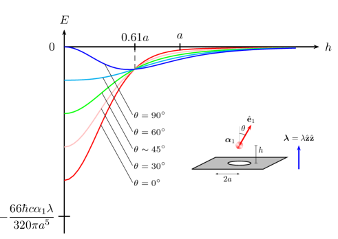
Figure 5: The energy of Eq. (49) is plotted as a function of height $h$ for an anisotropic atom above the center of a dielectric plate with an aperture of radius $a$ with polarizability in the direction of symmetry axis of plate as sketched in the insert. The curves correspond to different orientation $\theta$ of the atomic polarizability. All the curves have two orientation independent points for $h>0$ at $h\sim 0.61a$ and $h\sim 3.44a$, with the second orientation independent point visible only under sufficient zoom level.

V Point atom above a dielectric ring

The Casimir-Polder interaction energy between an atom and a dielectric, Eq. (24) in Eq. (41), is given by the expression

$$E=-\frac{\hbar c}{32\pi^{2}}\int d^{3}x\frac{1}{r^{7}}\Big{[}13\,\text{tr}({\bm{\alpha}}\cdot{\bm{\chi}})-56\,(\hat{\bf r}\cdot{\bm{\alpha}}\cdot{\bm{\chi}}\cdot\hat{\bf r})$$

$$\hskip 96.73936pt+63\,(\hat{\bf r}\cdot{\bm{\alpha}}\cdot\hat{\bf r})(\hat{\bf r}\cdot{\bm{\chi}}\cdot\hat{\bf r})\Big{]}$$ (50)

where

$${\bf r}={\bf x}-{\bf x}_{0},$$ (51)

${\bf x}_{0}$ being the position of the atom and ${\bf x}$ being the integral variable scanning the infinitesimal elements of the dielectric. The dielectric function for the atom is described by the atomic polarizability ${\bm{\alpha}}$ and the electric susceptibility for the interacting material is ${\bm{\chi}}$. We will confine our discussion to the retarded Casimir-Polder regime of Sec. III.3, where only the static zero frequency modes in polarizability contribute.

Let the ring be assumed to be on the $xy$-plane with its center at the origin. Thus, the electric susceptibility of the ring is

$${\bm{\chi}}={\bm{\sigma}}\delta(z-0)\delta(\rho-a),$$ (52)

where $a$ is the radius of the ring and ${\bm{\sigma}}$ is the polarizability of the ring. Let the atom with polarizability ${\bm{\alpha}}$ be positioned on the symmetry axis of the ring at a height $h$ above the center of the ring. Thus, the electric susceptibility of the atom is

$${\bm{\chi}}={\bm{\alpha}}\delta^{(3)}({\bf x}-{\bf x}_{0}),$$ (53)

where

$${\bf x}_{0}=h\,\hat{\bf z}.$$ (54)

See Fig. 6 for an illustrative diagram.

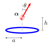
Figure 6: Point atom of polarizability ${\bm{\alpha}}$ above a dielectric ring of polarizability ${\bm{\sigma}}$. The atom is on the symmetry axis of the ring.

Since the atom is placed on the symmetry axis of the ring, we have the simplification

$${\bf r}=a\hat{\bm{\rho}}-h\hat{\bf z}$$ (55)

and

$$r=\sqrt{a^{2}+h^{2}},\qquad\hat{\bf r}=\frac{a\hat{\bm{\rho}}-h\hat{\bf z}}{\sqrt{a^{2}+h^{2}}}.$$ (56)

Thus, integrating over $\rho$ and $z$, the expression for the interaction energy in Eq. (50) takes the simplified form

$$E = -\frac{\hbar c}{32\pi^{2}}\frac{a}{(a^{2}+h^{2})^{\frac{7}{2}}}\int_{0}^{2\pi}d\phi\Big{[}13\,\text{tr}({\bm{\alpha}}\cdot{\bm{\sigma}})$$ (57)

$$-56\,(\hat{\bf r}\cdot{\bm{\alpha}}\cdot{\bm{\sigma}}\cdot\hat{\bf r})+63\,(\hat{\bf r}\cdot{\bm{\alpha}}\cdot\hat{\bf r})(\hat{\bf r}\cdot{\bm{\sigma}}\cdot\hat{\bf r})\Big{]}.\hskip 28.45274pt$$

We emphasize that the above expression assumes the following, (mostly for simplification in the ensuing analysis,) in addition to the approximations clarified in Section III.

1. We assume that the position of the point atom is exactly on the symmetry axis of the ring, while the orientations of the principal axes of polarizability are kept arbitrary. This puts a severe limitation if we were interested in the stability analysis of the atom.

2. We assume that the polarizability tensor of the ring is diagonal in the eigenbasis used to the characterize the geometry of the ring. These are chosen to be $\hat{\bf z}$, $\hat{\bm{\rho}}$, and $\hat{\bm{\phi}}$, with the direction of $\hat{\bf z}$ chosen along the symmetry axis of the ring. That is, we will assume that the polarizability tensor of the ring has the form

   $${\bm{\sigma}}=\sigma_{z}\,\hat{\bf z}\hat{\bf z}+\sigma_{\rho}\,\hat{\bm{\rho}}\hat{\bm{\rho}}+\sigma_{\phi}\,\hat{\bm{\phi}}\hat{\bm{\phi}}.$$ (58)

   We allow the polarizability tensor of the atom to be completely arbitrary,

   $${\bm{\alpha}}=\alpha_{1}\hat{\bf e}_{1}\hat{\bf e}_{1}+\alpha_{2}\hat{\bf e}_{2}\hat{\bf e}_{2}+\alpha_{3}\hat{\bf e}_{3}\hat{\bf e}_{3}.$$ (59)

Even with the above assumptions, the analysis involves sufficient number of parameters required to specify the anisotropies of the polarizations relative to the vector describing the distance between the materials. The principal axes for the ring are suitably chosen to be

$$\hat{\bm{\rho}} = \cos\phi\,\hat{\bf i}+\sin\phi\,\hat{\bf j},$$ (60a)

$$\hat{\bm{\phi}} = -\sin\phi\,\hat{\bf i}+\cos\phi\,\hat{\bf j},$$ (60b)

$$\hat{\bf z} = \hat{\bf k},$$ (60c)

which are unit vectors associated to the cylindrical polar coordinates. The principal axes for the atom are kept arbitrary to allow complete generality by choosing

$$\hat{\bf e}_{1} = \hat{\bf r}_{s},$$ (61a)

$$\hat{\bf e}_{2} = \cos\beta\,\hat{\bm{\phi}}_{s}+\sin\beta\,\hat{\bm{\theta}}_{s},$$ (61b)

$$\hat{\bf e}_{3} = -\sin\beta\,\hat{\bm{\phi}}_{s}+\cos\beta\,\hat{\bm{\theta}}_{s},$$ (61c)

where $\beta$ is an angle of rotation about the axes $\hat{\bf e}_{1}$. Unit vectors $\hat{\bf r}_{s}$, $\hat{\bm{\theta}}_{s}$, and $\hat{\bm{\phi}}_{s}$ are the unit vectors associated to the spherical polar coordinates,

$$\hat{\bf r}_{s} = \sin\theta\cos\phi_{s}\,\hat{\bf i}+\sin\theta\sin\phi_{s}\,\hat{\bf j}+\cos\theta\,\hat{\bf k},$$ (62a)

$$\hat{\bm{\theta}}_{s} = \cos\theta\cos\phi_{s}\,\hat{\bf i}+\cos\theta\sin\phi_{s}\,\hat{\bf j}-\sin\theta\,\hat{\bf k},$$ (62b)

$$\hat{\bm{\phi}}_{s} = -\sin\phi_{s}\,\hat{\bf i}+\cos\phi_{s}\,\hat{\bf j}.$$ (62c)

Since the axes $\hat{\bf e}_{1}$ need not be normal to the $x$-$y$ plane, we choose the spherical coordinate $\phi_{s}$ to be different from the cylindrical coordinate $\phi$. The configuration of an anisotropic atom above an anisotropic ring in terms of the above parameters involves the integration over the angle $\phi$, which renders the interaction energy to be dependent on the azimuth angle $\beta$ and independent of $\phi_{s}$ and $\phi$. This characteristic allows the choice $\phi_{s}=0$, however, we shall refrain and allow the algebra to bring out this feature explicitly.

V.1 Tangentially polarizable ring

To illustrate the anisotropic features of the interaction in Eq. (50) we begin by considering a special case. It will turn out that this case does not permit repulsion. Nevertheless, the associated simplification in the configuration brings out the role of anisotropy in the interaction.

Let the polarizability of the ring be purely in the tangential direction, that is,

$${\bm{\sigma}}=\sigma_{\phi}\,\hat{\bm{\phi}}\hat{\bm{\phi}},$$ (63)

where $\hat{\bm{\phi}}$ is a unit vector tangent to the ring. Then, because this vector is always perpendicular to the relative position vector ${\bf r}$,

$$\hat{\bm{\phi}}\cdot\hat{\bf r}=0,$$ (64)

using Eq. (56) we conclude that two of the three modes of interaction in Eq. (57) do not contribute. Thus, we have

$$E = -\frac{\hbar c\sigma_{\phi}}{32\pi^{2}}\frac{13a}{(a^{2}+h^{2})^{\frac{7}{2}}}\int_{0}^{2\pi}d\phi\,(\hat{\bm{\phi}}\cdot{\bm{\alpha}}\cdot\hat{\bm{\phi}}).$$ (65)

The construction $(\hat{\bm{\phi}}\cdot{\bm{\alpha}}\cdot\hat{\bm{\phi}})$ involves projection of the polarizability of the atom along one of the directions $\hat{\bm{\phi}}$ associated with the ring, and thus is independent of the height $h$. All the dependence in $h$ is contained in $1/(a^{2}+h^{2})^{7/2}$. Hence, we conclude that the energy is a monotonic function in its dependence in height $h$. This renders the component of the force on the atom in the direction of $\hat{\bf z}$ to be always attractive, because it is the negative derivative of energy with respect to $h$. That is, a ring that is polarizable only in the tangential direction always attracts a polarizable atom on the symmetry axis of the ring.

This conclusion leaves this particular case uninteresting in a discussion on the repulsive Casimir force. However, as we mentioned earlier, we shall carry out the discussion to a certain extent to highlight the role of anisotropy in these interactions.

V.1.1 Case: ${\bf\sigma}_{\phi}$ and $\alpha_{1}$

Let the polarizability of the atom be uniaxial in an arbitrary direction $\hat{\bf e}_{1}$ given by

$${\bm{\alpha}}=\alpha_{1}\,\hat{\bf e}_{1}\hat{\bf e}_{1}.$$ (66)

The interaction energy of Eq. (65) then takes the form

$$E = -\frac{\hbar c\alpha_{1}\sigma_{\phi}}{32\pi^{2}}\frac{13a}{(a^{2}+h^{2})^{\frac{7}{2}}}\int_{0}^{2\pi}d\phi\,(\hat{\bf e}_{1}\cdot\hat{\bm{\phi}})^{2}.$$ (67)

Using

$$\hat{\bf e}_{1}\cdot\hat{\bm{\phi}}=\sin\theta\sin(\phi_{s}-\phi)$$ (68)

we have

$$\int_{0}^{2\pi}d\phi\,(\hat{\bf e}_{1}\cdot\hat{\bm{\phi}})^{2}=\pi\sin^{2}\theta.$$ (69)

Thus, the interaction energy in Eq. (67) takes the form

$$E = -\frac{\hbar c\alpha_{1}\sigma_{\phi}}{32\pi}\frac{13a\sin^{2}\theta}{(a^{2}+h^{2})^{\frac{7}{2}}}.$$ (70)

The orientation dependence of the polarizability $\hat{\bf e}_{1}$ with respect to the symmetry axis $\hat{\bf z}$ is completely contained in $\sin^{2}\theta$. This is a generic feature. The interaction energy for permanent dipoles have an orientation dependence of the form $\cos\theta$ and that for polarizable atoms have orientation dependence of the form $\cos 2\theta=1-2\sin^{2}\theta$. The dependence on height $h$ is monotonic, and thus does not lead to repulsion.

V.1.2 Case: ${\bf\sigma}_{\phi}$ and $\alpha_{2}$

Next, let us assume the polarizability of the atom to be purely in the direction $\hat{\bf e}_{2}$, such that,

$${\bm{\alpha}}=\alpha_{2}\,\hat{\bf e}_{2}\hat{\bf e}_{2}.$$ (71)

Using

$$\hat{\bf e}_{2}\cdot\hat{\bm{\phi}}=\cos\beta\cos(\phi_{s}-\phi)+\cos\theta\sin\beta\sin(\phi_{s}-\phi)$$ (72)

we have

$$\int_{0}^{2\pi}d\phi\,(\hat{\bf e}_{2}\cdot\hat{\bm{\phi}})^{2}=\pi(\cos^{2}\beta+\cos^{2}\theta\sin^{2}\beta).$$ (73)

Thus, the interaction energy of Eq. (65) takes the form

$$E = -\frac{\hbar c\alpha_{2}\sigma_{\phi}}{32\pi}\frac{13a(\cos^{2}\beta+\cos^{2}\theta\sin^{2}\beta)}{(a^{2}+h^{2})^{\frac{7}{2}}}.$$ (74)

Note that for $\theta=0$ the interaction energy has azimuthal symmetry and is independent of $\beta$, which is expected. Observe that for $\beta=\pi/2$ and $\theta\to\theta-(\pi/2)$ in Eq. (74), we obtain the result for $\hat{\bf e}_{1}$ polarization in Eq. (70). This corresponds to the fact that, in Eqs. (61), a rotation about $\hat{\bf e}_{1}$ by an angle of $(\pi/2)-\beta$ and then a rotation about the new $\hat{\bf e}_{2}$ by $-\pi/2$ takes the direction of $\hat{\bf e}_{2}$ to $\hat{\bf e}_{1}$. In general the interaction energy for an atom is a linear combination of the plausible polarizabilities.

V.1.3 Case: ${\bf\sigma}_{\phi}$ and $\alpha_{3}$

Similarly, when the polarizability of the atom is purely in the direction $\hat{\bf e}_{3}$, such that

$${\bm{\alpha}}=\alpha_{3}\,\hat{\bf e}_{3}\hat{\bf e}_{3},$$ (75)

using

$$\hat{\bf e}_{3}\cdot\hat{\bm{\phi}}=-\sin\beta\cos(\phi_{s}-\phi)+\cos\theta\cos\beta\sin(\phi_{s}-\phi),$$ (76)

we have

$$\int_{0}^{2\pi}d\phi\,(\hat{\bf e}_{3}\cdot\hat{\bm{\phi}})^{2}=\pi(\sin^{2}\beta+\cos^{2}\theta\cos^{2}\beta).$$ (77)

Thus, the interaction energy of Eq. (65) takes the form

$$E = -\frac{\hbar c\alpha_{2}\sigma_{\phi}}{32\pi}\frac{13a(\sin^{2}\beta+\cos^{2}\theta\cos^{2}\beta)}{(a^{2}+h^{2})^{\frac{7}{2}}}.$$ (78)

Note that for $\theta=0$, the interaction energy has azimuthal symmetry. Further, we observe that the interaction energy for $\hat{\bf e}_{3}$ polarization in Eq. (78) is obtained from the interaction energy for $\hat{\bf e}_{2}$ polarization in Eq. (74) by the replacement $\beta\to\beta+(\pi/2)$. This is true in general because $\hat{\bf e}_{2}$ and $\hat{\bf e}_{3}$ are orthogonal vectors in the plane perpendicular to $\hat{\bf e}_{1}$, refer Eqs. (61), and are thus related by a ninety degree rotation in angle $\beta$.

V.2 Radially polarizable ring

Next, let the polarizability of the ring be purely in the radial direction,

$${\bm{\sigma}}=\sigma_{\rho}\,\hat{\bm{\rho}}\hat{\bm{\rho}},$$ (79)

where $\hat{\bm{\rho}}$ is a unit vector normal to the ring in the $x$-$y$ plane. The expression for the interaction energy in Eq. (57) can be expressed in the form

$$E = -\frac{\hbar c\sigma_{\rho}}{32\pi^{2}}\frac{a}{(a^{2}+h^{2})^{\frac{7}{2}}}\int_{0}^{2\pi}d\phi\Big{[}13(\hat{\bm{\rho}}\cdot{\bm{\alpha}}\cdot\hat{\bm{\rho}})$$ (80)

$$\hskip 14.22636pt-56(\hat{\bf r}\cdot{\bm{\alpha}}\cdot\hat{\bm{\rho}})(\hat{\bm{\rho}}\cdot\hat{\bf r})+63(\hat{\bf r}\cdot{\bm{\alpha}}\cdot\hat{\bf r})(\hat{\bm{\rho}}\cdot\hat{\bf r})^{2}\Big{]}.\hskip 14.22636pt$$

Using the representation for $\hat{\bf r}$ in Eq. (56) to evaluate $(\hat{\bm{\rho}}\cdot\hat{\bf r})$ we obtain

$$E = -\frac{\hbar c\sigma_{\rho}}{32\pi^{2}}\frac{a}{(a^{2}+h^{2})^{\frac{7}{2}}}\int_{0}^{2\pi}d\phi\bigg{[}13(\hat{\bm{\rho}}\cdot{\bm{\alpha}}\cdot\hat{\bm{\rho}})\hskip 39.83385pt$$ (81)

$$\hskip 42.67912pt-\frac{56a(\hat{\bf r}\cdot{\bm{\alpha}}\cdot\hat{\bm{\rho}})}{\sqrt{a^{2}+h^{2}}}+\frac{63a^{2}(\hat{\bf r}\cdot{\bm{\alpha}}\cdot\hat{\bf r})}{(a^{2}+h^{2})}\bigg{]}.\hskip 14.22636pt$$

V.2.1 Case: ${\bf\sigma}_{\rho}$ and $\alpha_{1}$

Let

$${\bm{\alpha}}=\alpha_{1}\,\hat{\bf e}_{1}\hat{\bf e}_{1}.$$ (82)

Now the relevant integrals involved are

$$\int_{0}^{2\pi}d\phi\,(\hat{\bf r}\cdot\hat{\bf e}_{1})(\hat{\bf e}_{1}\cdot\hat{\bm{\rho}})=\frac{\pi a\sin^{2}\theta}{\sqrt{a^{2}+h^{2}}}$$ (83)

and

$$\int_{0}^{2\pi}d\phi\,(\hat{\bf r}\cdot\hat{\bf e}_{1})^{2}=\frac{\pi(a^{2}\sin^{2}\theta+2h^{2}\cos^{2}\theta)}{(a^{2}+h^{2})}.$$ (84)

Using these integrals the interaction energy in Eq. (81) can be expressed in the form

$$E = -\frac{\hbar c\alpha_{1}\sigma_{\rho}}{32\pi}\frac{a}{(a^{2}+h^{2})^{\frac{11}{2}}}\Big{[}126h^{2}a^{2}\cos^{2}\theta$$ (85)

$$\hskip 28.45274pt+(20a^{4}-30h^{2}a^{2}+13h^{4})\sin^{2}\theta\Big{]}.\hskip 14.22636pt$$

This form for the interaction energy is useful to compare with other polarizabilities for the atom. Another suitable expression for interaction energy in Eq. (81), obtained using half-angle formulas for the trigonometric functions in Eq. (85), is

$$E = -\frac{\hbar c\alpha_{1}\sigma_{\rho}}{64\pi}\frac{a}{(a^{2}+h^{2})^{\frac{11}{2}}}\Big{[}(20a^{4}+96h^{2}a^{2}+13h^{4})$$ (86)

$$\hskip 28.45274pt-(20a^{4}-156h^{2}a^{2}+13h^{4})\cos 2\theta\Big{]}.$$

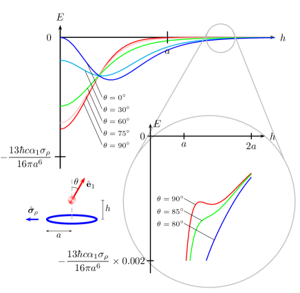
Figure 7: The interaction energy between an atom with polarizability ${\bm{\alpha}}=\alpha_{1}\,\hat{\bf e}_{1}\hat{\bf e}_{1}$ and a ring of polarizability ${\bm{\sigma}}=\sigma_{\rho}\,\hat{\bm{\rho}}\hat{\bm{\rho}}$ is illustrated in bottom left corner of figure. The energy in Eq. (86) is plotted as function of height $h$ for different orientations of $\hat{\bf e}_{1}$ with respect to the symmetry axis of the ring. The first repulsion occurs for $h\ll a$ when $\theta<43.43^{\circ}$. The inset provides a zoomed in view of the non-monotonicity, second region where the switch from attraction to repulsion occurs, which is not visible otherwise. Repulsive force experienced by the atom in the direction of the symmetry axis will be a manifestation of negative slopes in these plots.

Figure 7 is a plot of interaction energy in Eq. (86) as a function of height $h$ for different orientations $\theta$. The force of repulsion is the manifestation of energy trying to attain a minimum value, which is present whenever the energy plots have negative slopes. The regions with negative slope are orientation dependent, suggesting that anisotropy in the atom’s polarizability is important.

Let us investigate the orientation dependence of the interaction energy in Eq. (86). There exists a point at $h\sim 0.36a$ in Fig 7 where all the curves for different $\theta$ intersect. When the domain $h$ of the plot is extended further we encounter another such point at $h\sim 3.45a$, which has not been captured in Fig 7. These points for height $h$ are determined by the zeros of the polynomial that is coefficient of $\cos 2\theta$ in Eq. (86). That is,

$$13h^{4}-156h^{2}a^{2}+20a^{4}=0,$$ (87)

which have solutions

$$h=\pm a\sqrt{\frac{78\pm 8\sqrt{91}}{13}},$$ (88)

or, $h=\pm 0.36\,a$ and $h=\pm 3.45\,a$. For heights below the first torsion-free point, $h=0.36\,a$, the atom tries to orient itself vertically ($\theta=90^{\circ}$), because the energy is minimum for this orientation, then, for heights in between the two torsion-free points, in the range $0.36\,a<h<3.45\,a$, the atom tries to orient itself horizontally $(\theta=0$), and for heights beyond the second torsion-free point, beyond $3.45\,a<h$, the atom tries to orient itself vertically. This analysis suggests sudden transitions between orientations at torsion-free points without expense in energy, and could have applications in experiments involving a beam of polarizable atoms; for example, a beam of helium dimer. We shall postpone discussions of such applications to another occasion.

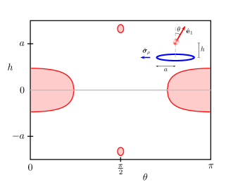
Figure 8: The shaded regions in the parameter space of height $h$ and orientation angle $\theta$ above leads to repulsion between an anisotropic atom with polarizability ${\bm{\alpha}}=\alpha_{1}\,\hat{\bf e}_{1}\hat{\bf e}_{1}$ interacting with a ring of polarizability ${\bm{\sigma}}=\sigma_{\rho}\,\hat{\bm{\rho}}\hat{\bm{\rho}}$, as illustrated in top right corner of figure and determined by Eq. (92).

The negative derivative of the energy in Eq. (86) with respect to height $h$ is the component of the force on the atom in the vertical direction, given by

$$F = -\frac{\hbar c\alpha_{1}\sigma_{\rho}}{64\pi}\frac{ha}{(a^{2}+h^{2})^{\frac{13}{2}}}\Big{[}(28a^{4}+812h^{2}a^{2}+91h^{4})$$ (89)

$$\hskip 28.45274pt-(532a^{4}-1456h^{2}a^{2}+91h^{4})\cos 2\theta\Big{]}.$$

For repulsion to occur the force on the atom must be positive. So, the condition for repulsion is established using the inequality

$$(28a^{4}+812h^{2}a^{2}+91h^{4})$$

$$\hskip 28.45274pt-(532a^{4}-1456h^{2}a^{2}+91h^{4})\cos 2\theta<0.$$ (90)

In the limit when the atom is very close to the center of the ring, only the $h\neq 0$ terms contribute. The atom experiences repulsion at the center of the ring when

$$\cos 2\theta>\frac{28}{512},$$ (91)

which amounts to $\theta<\frac{1}{2}\cos^{-1}(\frac{1}{19})\sim 43.43^{\circ}$. This is consistent with plots in Fig 7. For general orientation $\theta$, we have repulsive regions at height $h$ given by the inequality

$$\frac{h}{a}<\pm\sqrt{\frac{-(812+1456\cos{2\theta})\pm\sqrt{D}}{182(1-\cos{2\theta})}},$$ (92)

where

$$D = (812+1456\cos{2\theta})^{2}$$ (93)

$$-364(1-\cos{2\theta})(28-532\cos{2\theta}).$$

The solutions above are real for $D>0$. This condition allows us to find a range of orientations for which repulsion is possible. That is, the discriminant $D=0$ determines a condition on angle $\theta$ for repulsion. This is given by the inequality obtained by simplifying Eq. (93),

$$92+364\cos{2\theta}+273\cos^{2}{2\theta}>0.$$ (94)

We find $86.98^{\circ}<\theta<93.02^{\circ}$ to be a range of orientations allowing repulsion. Using $h=0$, we also find $-43.43^{\circ}<\theta<43.43^{\circ}$ and $136.57<\theta<223.43^{\circ}$ to be orientations plausible for repulsion. In Fig. 8, we plot these repulsively interacting regions in parameter space, determined by Eq. (92).

V.2.2 Case: ${\bf\sigma}_{\rho}$ and $\alpha_{2}$

Let

$${\bm{\alpha}}=\alpha_{2}\,\hat{\bf e}_{2}\hat{\bf e}_{2}.$$ (95)

The relevant integrals involved are

$$\int_{0}^{2\pi}d\phi\,(\hat{\bf r}\cdot\hat{\bf e}_{2})(\hat{\bf e}_{2}\cdot\hat{\bm{\rho}})=\frac{\pi a(\cos^{2}\beta+\sin^{2}\beta\cos^{2}\theta)}{\sqrt{a^{2}+h^{2}}}$$ (96)

and

$$\int_{0}^{2\pi}d\phi\,(\hat{\bf r}\cdot\hat{\bf e}_{2})^{2} = \frac{\pi a^{2}(\cos^{2}\beta+\sin^{2}\beta\cos^{2}\theta)}{(a^{2}+h^{2})}$$ (97)

$$+\frac{2\pi h^{2}\sin^{2}\beta\sin^{2}\theta)}{(a^{2}+h^{2})}.$$

Using these integrals, we determine the interaction energy in Eq. (81) to be

$$E=-\frac{\hbar c\alpha_{2}\sigma_{\rho}}{32\pi}\frac{a}{(a^{2}+h^{2})^{\frac{11}{2}}}\Big{[}126h^{2}a^{2}\sin^{2}\beta\sin^{2}\theta\hskip 28.45274pt$$

$$\hskip 8.53581pt+(20a^{4}-30h^{2}a^{2}+13h^{4})(\cos^{2}\beta+\sin^{2}\beta\cos^{2}\theta)\Big{]}.$$ (98)

The expression for energy in Eq. (98) has the same properties under rotations discussed after Eq. (74). Thus, for $\beta=\pi/2$ and $\theta\to\theta-(\pi/2)$, the energy in Eq. (98) becomes the energy for $\hat{\bf e}_{1}$ polarization in Eq. (85).

V.2.3 Case: ${\bf\sigma}_{\rho}$ and $\alpha_{3}$

Let

$${\bm{\alpha}}=\alpha_{3}\,\hat{\bf e}_{3}\hat{\bf e}_{3}.$$ (99)

The interaction energy for this case is given by

$$E=-\frac{\hbar c\alpha_{3}\sigma_{\rho}}{32\pi}\frac{a}{(a^{2}+h^{2})^{\frac{11}{2}}}\Big{[}126h^{2}a^{2}\cos^{2}\beta\sin^{2}\theta\hskip 28.45274pt$$

$$\hskip 8.53581pt+(20a^{4}-30h^{2}a^{2}+13h^{4})(\sin^{2}\beta+\cos^{2}\beta\cos^{2}\theta)\Big{]}.\hskip 22.76219pt$$ (100)

This result is obtained from the case of $\hat{\bf e}_{2}$ polarization by a rotation of ninety degrees about the $\hat{\bf e}_{3}$, which is obtained by the replacement $\beta\to(\pi/2)-\beta$ and swapping $\cos\beta\leftrightarrow\sin\beta$, as observed after Eq. (78).

V.3 Ring polarizable about its symmetry axis

Finally, let the polarizability of the ring be purely along the symmetry axis of the ring, chosen to be $\hat{\bf z}$,

$${\bm{\sigma}}=\sigma_{z}\,\hat{\bf z}\hat{\bf z}.$$ (101)

The expression for the interaction energy is of the form

$$E = -\frac{\hbar c\sigma_{z}}{32\pi^{2}}\frac{a}{(a^{2}+h^{2})^{\frac{7}{2}}}\int_{0}^{2\pi}d\phi\Big{[}13(\hat{\bf z}\cdot{\bm{\alpha}}\cdot\hat{\bf z})$$ (102)

$$\hskip 14.22636pt-56(\hat{\bf r}\cdot{\bm{\alpha}}\cdot\hat{\bf z})(\hat{\bf z}\cdot\hat{\bf r})+63(\hat{\bf r}\cdot{\bm{\alpha}}\cdot\hat{\bf r})(\hat{\bf z}\cdot\hat{\bf r})^{2}\Big{]}.\hskip 14.22636pt$$

Using Eq. (56) to evaluate $(\hat{\bf z}\cdot\hat{\bf r})$, we obtain

$$E = -\frac{\hbar c\sigma_{z}}{32\pi^{2}}\frac{a}{(a^{2}+h^{2})^{\frac{7}{2}}}\int_{0}^{2\pi}d\phi\bigg{[}13(\hat{\bf z}\cdot{\bm{\alpha}}\cdot\hat{\bf z})\hskip 39.83385pt$$ (103)

$$\hskip 42.67912pt-\frac{56h(\hat{\bf r}\cdot{\bm{\alpha}}\cdot\hat{\bf z})}{\sqrt{a^{2}+h^{2}}}+\frac{63h^{2}(\hat{\bf r}\cdot{\bm{\alpha}}\cdot\hat{\bf r})}{(a^{2}+h^{2})}\bigg{]}.\hskip 14.22636pt$$

V.3.1 Case: ${\bf\sigma}_{z}$ and $\alpha_{1}$

Let

$${\bm{\alpha}}=\alpha_{1}\,\hat{\bf e}_{1}\hat{\bf e}_{1}.$$ (104)

The relevant integrals involved are

$$\int_{0}^{2\pi}d\phi\,(\hat{\bf z}\cdot\hat{\bf e}_{1})^{2} = 2\pi\cos^{2}\theta,$$ (105a)

$$\int_{0}^{2\pi}d\phi\,(\hat{\bf r}\cdot\hat{\bf e}_{1})(\hat{\bf e}_{1}\cdot\hat{\bf z}) = -\frac{2\pi h\cos^{2}\theta}{\sqrt{a^{2}+h^{2}}},$$ (105b)

$$\int_{0}^{2\pi}d\phi\,(\hat{\bf r}\cdot\hat{\bf e}_{1})^{2} = \frac{\pi(a^{2}\sin^{2}\theta+2h^{2}\cos^{2}\theta)}{(a^{2}+h^{2})}.\hskip 25.60747pt$$ (105c)

Using these integrals, the interaction energy in Eq. (103) can be expressed in the form

$$E = -\frac{\hbar c\alpha_{1}\sigma_{z}}{32\pi}\frac{a}{(a^{2}+h^{2})^{\frac{11}{2}}}\Big{[}63h^{2}a^{2}\sin^{2}\theta$$ (106)

$$\hskip 28.45274pt+(26a^{4}-60h^{2}a^{2}+40h^{4})\cos^{2}\theta\Big{]}.\hskip 14.22636pt$$

The differences between the interaction energy expressions for the radially polarizable ring in Eq. (85) and axially polarizable ring in Eq. (106) are insightful and brings out the source of separate contributions to the interaction energy. Using half-angle formulas for the trigonometric functions in Eq. (106), we can express the interaction energy in the form

$$E = -\frac{\hbar c\alpha_{1}\sigma_{z}}{64\pi}\frac{a}{(a^{2}+h^{2})^{\frac{11}{2}}}\Big{[}(26a^{4}+3h^{2}a^{2}+40h^{4})$$ (107)

$$\hskip 28.45274pt+(26a^{4}-123h^{2}a^{2}+40h^{4})\cos 2\theta\Big{]}.$$

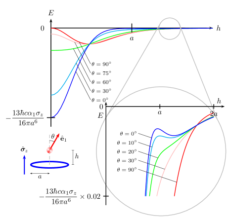
Figure 9: The interaction energy of Eq. (107) is plotted as function of height $h$ for different orientations $\theta$. The atom has polarizability ${\bm{\alpha}}=\alpha_{1}\,\hat{\bf e}_{1}\hat{\bf e}_{1}$ and the ring has polarizability ${\bm{\sigma}}=\sigma_{z}\,\hat{\bf z}\hat{\bf z}$, as illustrated in bottom left corner of figure. The inset provides a zoomed-in view of the non-monotonicity.

In Fig. 9, we plot the interaction energy of Eq. (107) as a function of height $h$ for various orientations $\theta$. The general features of the plot in Fig. 9 for the axial polarization of ring imitates that of the plot in Fig. 7 for the radial polarization of ring. The specifics of the interaction are different, but the qualitative features are the same. A striking difference is that for the radial polarization the energy is minimized at $h=0$ for $\theta=90^{\circ}$, while for the axial polarization the energy is minimized at $h=0$ for $\theta=0$. That is, for both $h=0$ and $h\to\infty$, the atom tries to align its polarization with that of the ring.

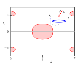
Figure 10: The shaded regions in the parameter space of height $h$ and orientation angle $\theta$ above leads to repulsion between an anisotropic atom with polarizability ${\bm{\alpha}}=\alpha_{1}\,\hat{\bf e}_{1}\hat{\bf e}_{1}$ interacting with a ring of polarizability ${\bm{\sigma}}=\sigma_{z}\,\hat{\bf z}\hat{\bf z}$, as illustrated in top right corner of figure.

The heights for which the interaction energy is orientation independent is given by the zeros of

$$26a^{4}-123h^{2}a^{2}+40h^{4}=0,$$ (108)

with solutions

$$h=\pm a\sqrt{\frac{123\pm\sqrt{10969}}{80}},$$ (109)

at $h=\pm 0.48\,a$ and $h=\pm 1.69\,a$. The expression for the component of the force along the symmetry axis is

$$F = -\frac{\hbar c\alpha_{1}\sigma_{z}}{64\pi}\frac{7ha}{(a^{2}+h^{2})^{\frac{13}{2}}}\Big{[}(40a^{4}-19h^{2}a^{2}+40h^{4})$$ (110)

$$\hskip 28.45274pt+(76a^{4}-181h^{2}a^{2}+40h^{4})\cos 2\theta\Big{]}.$$

The repulsive regions in height $h$ is given by the inequality

$$\frac{h}{a}<\pm\sqrt{\frac{(19+181\cos{2\theta})\pm\sqrt{D}}{80(1+\cos{2\theta})}}$$ (111)

where

$$D = (19+181\cos{2\theta})^{2}$$ (112)

$$-160(1+\cos{2\theta})(40+76\cos{2\theta})$$

$$= -6039-11682\cos 2\theta+20601\cos^{2}2\theta.$$

The critical angles of the orientations for which repulsion begins is determined by $D=0$. This shows that repulsion only occurs when $0<\theta<13.27^{\circ}$ and $166.73<\theta<180^{\circ}$. The other critical value is determined by $h\to 0$, given by

$$\cos 2\theta=-\frac{40}{76},$$ (113)

which has solutions $60.88^{\circ}<\theta<119.12^{\circ}$.

V.3.2 Case: ${\bf\sigma}_{z}$ and $\alpha_{2}$

For

$${\bm{\alpha}}=\alpha_{2}\,\hat{\bf e}_{2}\hat{\bf e}_{2},$$ (114)

the interaction energy in Eq. (103) can be expressed in the form

$$E = -\frac{\hbar c\alpha_{2}\sigma_{z}}{32\pi}\frac{a}{(a^{2}+h^{2})^{\frac{11}{2}}}\Big{[}63h^{2}a^{2}(\cos^{2}\beta+\sin^{2}\beta\cos^{2}\theta)$$ (115)

$$\hskip 28.45274pt+(26a^{4}-60h^{2}a^{2}+40h^{4})\sin^{2}\beta\sin^{2}\theta\Big{]}.\hskip 14.22636pt$$

The orientation dependence in this energy should be compared with that for the radial polarization in Eq. (98).

V.3.3 Case: ${\bf\sigma}_{z}$ and $\alpha_{3}$

For

$${\bm{\alpha}}=\alpha_{3}\,\hat{\bf e}_{3}\hat{\bf e}_{3},$$ (116)

the interaction energy in Eq. (103) can be expressed in the form

$$E = -\frac{\hbar c\alpha_{3}\sigma_{z}}{32\pi}\frac{a}{(a^{2}+h^{2})^{\frac{11}{2}}}\Big{[}63h^{2}a^{2}(\sin^{2}\beta+\cos^{2}\beta\cos^{2}\theta)$$ (117)

$$\hskip 28.45274pt+(26a^{4}-60h^{2}a^{2}+40h^{4})\cos^{2}\beta\sin^{2}\theta\Big{]}.\hskip 14.22636pt$$

Again, the orientation dependence in this expression should be contrasted with that in Eq. (100).

V.4 Partially isotropic ring

If the polarizability of the ring is isotropic in the $x$-$y$ plane we have

$${\bm{\sigma}}=\sigma\,(\hat{\bm{\rho}}\hat{\bm{\rho}}+\hat{\bm{\phi}}\hat{\bm{\phi}}).$$ (118)

The interaction energy for this case will be a linear sum of the individual energies for the radially and tangentially polarizable cases. If the polarizability of the atom is of the form

$${\bm{\alpha}}=\alpha_{1}\,\hat{\bf e}_{1}\hat{\bf e}_{1},$$ (119)

the interaction energy is obtained by adding the energies in Eqs. (70) and (86).

$$E = -\frac{\hbar c\alpha_{1}\sigma}{64\pi}\frac{a}{(a^{2}+h^{2})^{\frac{11}{2}}}\Big{[}(33a^{4}+122h^{2}a^{2}+26h^{4})$$ (120)

$$\hskip 28.45274pt-(33a^{4}-130h^{2}a^{2}+26h^{4})\cos 2\theta\Big{]}.$$

We see that the qualitative features do not change relative to that of a radially polarizable ring. It is of interest to inquire how the features of energy plot change from a ring to that of a plate. To this end, we study a polarizable annular disc.

VI Polarizable atom above a dielectric annular disc

Consider a polarizable annular disc of inner radius $a$ and outer radius $b$, with polarizability described by

$${\bm{\chi}}={\bm{\lambda}}\delta(z)\theta(\rho-a)\theta(b-\rho).$$ (121)

In the limit $b\to\infty$ this corresponds to a plate of infinite extent with a circular aperture of radius $a$. In the limit $a\to 0$ this corresponds to circular disc of radius $b$. In the simple limit $b\to a$ the annular disc is of course non existent. However, the delicate limit of $b\to a$ in conjunction with $\lambda\to\infty$ such that

$$\sigma=\lambda(b-a)$$ (122)

is kept fixed, leads to a construction of an infinitely thin ring, after recognizing the $\delta$-function representation in terms of step functions

$$\delta(\rho-a)=\lim_{b\to a}\frac{\theta(b-\rho)\theta(\rho-a)}{(b-a)}.$$ (123)

In this manner, we can obtain the results for ring, and that for plate with circular aperture, from the results for an annular disc.

VI.1 Partially isotropic annular disc

Let the polarizability of the atom be of the form

$${\bm{\alpha}}=\alpha_{1}\,\hat{\bf e}_{1}\hat{\bf e}_{1}.$$ (124)

Let the annular disc be isotropically polarizable in the $x$-$y$ plane,

$${\bm{\lambda}}=\lambda{\bf 1}_{\perp}=\lambda(\hat{\bf x}\hat{\bf x}+\hat{\bf y}\hat{\bf y})=\lambda(\hat{\bm{\rho}}\hat{\bm{\rho}}+\hat{\bm{\phi}}\hat{\bm{\phi}}).$$ (125)

Then, the expression for the interaction energy in Eq. (50) takes the simplified form

$$E = -\frac{\hbar c\alpha_{1}\lambda}{32\pi^{2}}\int_{a}^{b}d\rho\frac{\rho}{(\rho^{2}+h^{2})^{\frac{7}{2}}}\int_{0}^{2\pi}d\phi\Big{[}13(\hat{\bf e}_{1}\cdot{\bf 1}_{\perp}\cdot\hat{\bf e}_{1})$$ (126)

$$-56\,(\hat{\bf r}\cdot\hat{\bf e}_{1})(\hat{\bf e}_{1}\cdot{\bf 1}_{\perp}\cdot\hat{\bf r})+63\,(\hat{\bf r}\cdot\hat{\bf e}_{1})^{2}(\hat{\bf r}\cdot{\bf 1}_{\perp}\cdot\hat{\bf r})\Big{]}.\hskip 22.76219pt$$

Completing the integral in $\phi$ we obtain

$$E = -\frac{\hbar c\alpha_{1}\lambda}{64\pi}\int_{a}^{b}d\rho\frac{\rho}{(\rho^{2}+h^{2})^{\frac{11}{2}}}\Big{[}(33\rho^{4}+122h^{2}\rho^{2}+26h^{4})$$ (127)

$$\hskip 28.45274pt-(33\rho^{4}-130h^{2}\rho^{2}+26h^{4})\cos 2\theta\Big{]}.$$

In the limit $\lambda\to\infty$ and $b\to a$ such that $\lambda(b-a)=\sigma$ we have $\lambda\int_{a}^{b}d\rho\to\sigma$, which then leads to the interaction energy for a partially isotropic ring in Eq. (120). Completing the integral in $\rho$ Eq. (127) leads to

$$E = -\frac{\hbar c\alpha_{1}\lambda}{320\pi}\frac{(-1)}{(\rho^{2}+h^{2})^{\frac{9}{2}}}\Big{[}(33\rho^{4}+106h^{2}\rho^{2}+38h^{4})$$ (128)

$$\hskip 28.45274pt-(33\rho^{4}-74h^{2}\rho^{2}-2h^{4})\cos 2\theta\Big{]}\bigg{|}^{\rho=b}_{\rho=a}.$$

In the limit $b\to\infty$, this reproduces the expression for the energy of an infinite plate with a circular aperture in Eq. (45).

The characteristic features of the interaction energy for an annular disc in Eq. (128) are similar to those of a partially isotropic ring in Eq. (120). These are, the two orientation independent torsion free heights on each side of the disc, and the orientation preferences at $h=0$ and $h\to\infty$. The orientation independent heights are determined by setting the coefficient of the term with $\cos 2\theta$ to zero in Eq. (128). That is,

$$\frac{(33b^{4}-74b^{2}h^{2}-2h^{4})}{(b^{2}+h^{2})^{\frac{9}{2}}}-\frac{(33a^{4}-74a^{2}h^{2}-2h^{4})}{(a^{2}+h^{2})^{\frac{9}{2}}}=0,$$ (129)

which has four solutions for $h$. Two of the solutions are above the disc ($h>0$), and the other two are opposite in sign and symmetrically below the disc. Denoting the positive solutions as $h_{1}$ and $h_{2}$, we find

$$0.52a\xleftarrow[\text{ring}]{a\leftarrow b}h_{1}\xrightarrow[\text{plate}]{b\to\infty}0.66a$$ (130a)

and

$$2.18a\xleftarrow[\text{ring}]{a\leftarrow b}h_{2}\xrightarrow[\text{plate}]{b\to\infty}\infty,$$ (130b)

such that $h_{1}$ and $h_{2}$ vary monotonically. At $h=0$ the orientation preference of the atom is to direct its polarizability in the plane of the plate ($\theta=90^{\circ}$). As the atom is moved away from this position along the axis, the orientation preference abruptly switches to $\theta=0$ as the atom crosses the height $h=h_{1}$. Afterwards it switches back to $\theta=90^{\circ}$ when we cross the height $h=h_{2}$. The existence of two orientation independent heights, on each side of disc, thus guarantees that the orientation preference at $h=0$ will be the same as the orientation preference at $h\to\infty$. Conversely, since the plate ($b\to\infty$) has only one orientation independent height, the other being at infinity, see Eq. (130b), the implication is that orientation preference of the atom at $h=0$ is orthogonal to that at $h\to\infty$.

VI.2 Radially polarizable annular disc

For a polarizable atom on the symmetry axis of an annular disc that is polarizable radially,

$${\bm{\lambda}}=\lambda_{\rho}\hat{\bm{\rho}}\hat{\bm{\rho}},$$ (131)

the interaction energy is

$$E = -\frac{\hbar c\alpha_{1}\lambda_{\rho}}{64\pi}\frac{(-1)}{(\rho^{2}+h^{2})^{\frac{9}{2}}}\Big{[}(4\rho^{4}+16h^{2}\rho^{2}+5h^{4})$$ (132)

$$\hskip 28.45274pt-(4\rho^{4}-20h^{2}\rho^{2}-3h^{4})\cos 2\theta\Big{]}\bigg{|}^{\rho=b}_{\rho=a}.$$

This expression tends to the expression for a ring in Eq. (86), and to the expression for a plate in Eq. (47), in the limits $b\to a$ and $b\to\infty$, respectively.

The characteristic features of the interaction energy in Eq. (132) for radially polarizable annular disc qualitatively mimics that of partially isotropically polarizable annular disc in Eq. (128). The orientation independent heights are now determined by

$$\frac{(4b^{4}-20b^{2}h^{2}-3h^{4})}{(b^{2}+h^{2})^{\frac{9}{2}}}-\frac{(4a^{4}-20a^{2}h^{2}-3h^{4})}{(a^{2}+h^{2})^{\frac{9}{2}}}=0,$$ (133)

which again has four solutions. Two of the solutions above the disc, ($h_{1}$ and $h_{2}$, with $0<h_{1}<h_{2}$), are

$$0.36a\xleftarrow[\text{ring}]{a\leftarrow b}h_{1}\xrightarrow[\text{plate}]{b\to\infty}0.44a$$ (134a)

and

$$3.45a\xleftarrow[\text{ring}]{a\leftarrow b}h_{2}\xrightarrow[\text{plate}]{b\to\infty}\infty.$$ (134b)

Again, the existence of two positive orientation independent heights for the case of annular disc, and for the limiting case of disc becoming a ring, implies that the orientation preference of the atom at $h=0$ and $h\to\infty$ is the same. In the limiting case of an annular disc becoming an annular plate one of the orientation independent heights moves to infinity, which implies that the orientation preference at $h=0$ is orthogonal to that at $h\to\infty$ for an annular plate. These points have been illustrated in Fig. 11.

Orientation		Criteria for second region of repulsion
$\theta=90^{\circ}$		$a<b<1.257a$
$\theta=88.2^{\circ}$		$a<b<1.201a$
$\theta=87.3^{\circ}$		$a<b<1.107a$

Table 1: This table lists the criteria when the region of repulsion for intermediate distances can occur between an anisotropically polarizable annular disc and anisotropically polarizable atom for certain orientations. The left column gives the orientation of the atom deviating away from the symmetry axis when the disc is polarizable in the radial direction. The right column gives the criteria for second region of repulsion to be present. The corresponding chart for axially polarizable annular disc has been presented in Ref. Marchetta et al. (2020).

A motivation for analyzing the disc was to determine when does the second region of repulsion emerge in the transition of the annular disc shrinking down to a ring. These values have been evaluated numerically and are listed in Table 1.

VI.3 Axially polarizable annular disc

When the annular disc is polarizable along the direction of the symmetry axis of the disc,

$${\bm{\lambda}}=\lambda_{z}\hat{\bf z}\hat{\bf z},$$ (135)

the interaction energy is

$$E = -\frac{\hbar c\alpha_{1}\lambda_{z}}{64\pi}\frac{1}{5}\frac{(-1)}{(\rho^{2}+h^{2})^{\frac{9}{2}}}\Big{[}(26\rho^{4}+17h^{2}\rho^{2}+26h^{4})$$ (136)

$$\hskip 28.45274pt+(26\rho^{4}-73h^{2}\rho^{2}+6h^{4})\cos 2\theta\Big{]}\bigg{|}^{\rho=b}_{\rho=a}.$$

The expression for a ring in Eq. (107), and the expression for a plate in Eq. (49), are reproduced from the interaction energy of Eq. (136) in the limits $b\to a$ and $b\to\infty$, respectively.

The orientation independent heights are now determined by

$$\frac{(26b^{4}-73b^{2}h^{2}+6h^{4})}{(b^{2}+h^{2})^{\frac{9}{2}}}-\frac{(26a^{4}-73a^{2}h^{2}+6h^{4})}{(a^{2}+h^{2})^{\frac{9}{2}}}=0,$$ (137)

with the solutions above the disc satisfying

$$0.48a\xleftarrow[\text{ring}]{a\leftarrow b}h_{1}\xrightarrow[\text{plate}]{b\to\infty}0.60a$$ (138a)

and

$$1.69a\xleftarrow[\text{ring}]{a\leftarrow b}h_{2}\xrightarrow[\text{plate}]{b\to\infty}3.44a.$$ (138b)

Unlike the case of radial polarizability, here, two orientation independent heights on each side of disc exists even in the limit when the disc becomes a plate. That is, the second orientation independent height does not move away to infinity in the limiting case of a plate. This implies that the orientation preference of the atom at $h=0$ and $h\to\infty$ is the same. See illustration in Fig. 11. This should be contrasted with that of radially polarizable disc in which case the orientation preference of the polarizability of the atom at $h=0$ is orthogonal to that at $h\to\infty$.

VII Summary of results

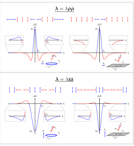
Figure 11: Difference in interaction energy $\Delta E$ between $\theta=0$ and $\theta=\pi/2$ plotted as a function of height $h$. The intersection of the energy curves with abscissa represent orientation independent points, marked $h_{1}$ and $h_{2}$. The orientation dependence at each height is shown as double-arrowed vectors adjacent to the horizontal axis. Observe that the orientation preferences for the plate is different for radial and axial polarizabilities.

Admittedly, we have considered too many cases and it has been hard to keep track. A brief summary of our results in this paper has been presented in Ref. Marchetta et al. (2020). We already pointed out that the qualitative features of isotropically polarizability in a plane is identical to that of radially polarizable case. We have also emphasized that the characteristic features of the interaction energy are the orientation independent heights and the orientation preferences at $h=0$ and $h=\infty$. To this end, we feel it is sufficient to bring out the difference between the radially polarizable case and the axially polarizable case.

We summarize the limiting forms of the expressions for interaction energy for radial polarization as

$${\bm{\lambda}}=\lambda\hat{\bm{\rho}}\hat{\bm{\rho}}:\qquad\text{Eq.\,(\ref{CPannD-e1lr-apr})}\begin{cases}\xrightarrow[\text{ring}]{b\to a}\text{Eq.\,(\ref{intE-e1lr})}\\[19.91692pt] \xrightarrow[\text{plate}]{b\to\infty}\text{Eq.\,(\ref{energy-atom-plate-hole-lr})}\end{cases}$$ (139a)

and

Eq. (86) $$\begin{cases}\xrightarrow{h\to 0}-E_{r}20(1-\cos 2\theta),\\[8.53581pt] \xrightarrow{h\to\infty}-E_{r}\dfrac{a^{7}}{h^{7}}13(1-\cos 2\theta),\end{cases}$$ (139b)

Eq. (47) $$\begin{cases}\xrightarrow{h\to 0}-E_{p}4(1-\cos 2\theta),\\[8.53581pt] \xrightarrow{h\to\infty}-E_{p}\dfrac{a^{5}}{h^{5}}(5+3\cos 2\theta),\end{cases}$$ (139c)

where

$$E_{r}=\frac{\hbar c\alpha_{1}\sigma_{\rho}}{64\pi a^{6}},\qquad E_{p}=\frac{\hbar c\alpha_{1}\lambda_{\rho}}{64\pi a^{5}}.$$ (140)

The difference in the orientation dependence between the plate and the ring arises because minimum energy for a ring at $h\to\infty$ is decided by

$$-(1-\cos 2\theta)=\begin{cases}0,&\theta=0,\\ -2,&\theta=90^{\circ},\end{cases}$$ (141)

and the minimum energy for a plate at $h\to\infty$ is decided by

$$-(5+3\cos 2\theta)=\begin{cases}-8,&\theta=0,\\ -2,&\theta=90^{\circ}.\end{cases}$$ (142)

The source of this, again, can be attributed to the dyadic-dyadic interaction.

We repeat the summary for axial polarizability as

$${\bm{\lambda}}=\lambda\hat{\bf z}\hat{\bf z}:\qquad\text{Eq.\,(\ref{CPannD-e1lz-apr})}\begin{cases}\xrightarrow[\text{ring}]{b\to a}\text{Eq.\,(\ref{intE-e1lz})}\\[19.91692pt] \xrightarrow[\text{plate}]{b\to\infty}\text{Eq.\,(\ref{energy-atom-plate-hole-lz})}\end{cases}$$ (143a)

and

Eq. (107) $$\begin{cases}\xrightarrow{h\to 0}-E_{r}26(1+\cos 2\theta),\\[8.53581pt] \xrightarrow{h\to\infty}-E_{r}\dfrac{a^{7}}{h^{7}}40(1+\cos 2\theta),\end{cases}$$ (143b)

Eq. (49) $$\begin{cases}\xrightarrow{h\to 0}-\dfrac{E_{p}}{5}26(1+\cos 2\theta),\\[8.53581pt] \xrightarrow{h\to\infty}-\dfrac{E_{p}}{5}\dfrac{a^{5}}{h^{5}}(26+6\cos 2\theta),\end{cases}$$ (143c)

where $E_{r}$ and $E_{p}$ are now given by Eq. (140) after swapping the subscripts $\rho\to z$. Identical orientation dependence between the plate and the ring in this case arises because minimum energy for a ring at $h\to\infty$ is decided by

$$-40(1+\cos 2\theta)=\begin{cases}-80,&\theta=0,\\ 0,&\theta=90^{\circ},\end{cases}$$ (144)

and the minimum energy for a plate at $h\to\infty$ is decided by

$$-(26+6\cos 2\theta)=\begin{cases}-32,&\theta=0,\\ -20,&\theta=90^{\circ}.\end{cases}$$ (145)

The source of this can be attributed to the dyadic-dyadic interaction, which is short of an intuitive understanding.

We plotted the energy difference between orientations at $\theta=0^{\circ}$ and $\theta=90^{\circ}$ to highlight the orientation independent heights and the orientation dependence with respect to heights in Fig. 11. Among the four plots, note that for the case of radially polarizable plate, the atom tends to orient itself perpendicular to the direction of polarizability of the plate for $h\to\infty$. This contrasting feature is the key result of our analysis. We envision a beam of polarizable atoms passing through an aperture in a dielectric plate as an application that will exploit our result.

VIII Casimir machine

A rotaxane Anelli et al. (1991) is a molecular structure consisting of a ring shaped molecule free to move on another dumbbell shaped molecule. A rotaxane is a machine because the position of the ring can be controlled by expending chemical or electrostatic energy to change the associated interaction energy between the ‘ring’ and the ‘dumbbell’. These structures have been studied with considerable interest to find applications in constructing molecular machines Balzani et al. (2008). Using results from Sec. V.3.1, we propose a prototype for a rotaxane-like machine using the configurations studied there. An illustrative diagram of such a machine is shown in Fig. 12. Casimir-Polder approximation typically require the distances to be in the ballpark of 100 nm, and thus our discussion here is applicable for plausible applications in nanotechnology. The proposal here is superficial and presented for the sake of captivating interest, in the sense that careful details in the specific design has not been attended.

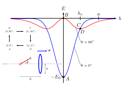
Figure 12: A prototype of a Casimir machine. Controlling the orientation $\theta$ of the polarizability of the nanoparticle allows the movement of the polarizable ring along the symmetry axis. For angle $\theta=0$ it is energetically favorable for the nanoparticle to be at the center of the ring, and for $\theta=90^{\circ}$ it is repelled from the ring. The plot is the interaction energy of the nanoparticle and ring as a function of height $h$ for $\theta=0$ and $\theta=90^{\circ}$. The configuration states, $A$, $B$, $C$, and $D$, in the Casimir machine are marked on the plots and illustrated in the insets.

We consider a polarizable ring and a polarizable atom with interaction energy given by Eq. (107) rewritten here in the form

$$E(h,\theta) = -\frac{E_{0}}{52}\frac{a^{7}}{(a^{2}+h^{2})^{\frac{11}{2}}}\Big{[}(26a^{4}+3h^{2}a^{2}+40h^{4})\hskip 8.53581pt$$ (146)

$$\hskip 14.22636pt+(26a^{4}-123h^{2}a^{2}+40h^{4})\cos 2\theta\Big{]},$$

where $E_{0}=13\hbar c\alpha\sigma/(16\pi a^{6})$. This energy has been plotted with respect to height $h$ in Fig. 12 for $\theta=0$ and $\theta=90^{\circ}$. Let us assume that the atom is constrained to move on the axis. The force between the atom and ring is given by

$$F=-\frac{\partial E}{\partial h}$$ (147)

and can be expressed in the form

$$F(h,\theta) = -\frac{F_{0}}{52}\frac{7a^{8}h}{(a^{2}+h^{2})^{\frac{13}{2}}}\Big{[}(40a^{4}-19h^{2}a^{2}+40h^{4})\hskip 8.53581pt$$ (148)

$$\hskip 14.22636pt+(76a^{4}-181h^{2}a^{2}+40h^{4})\cos 2\theta\Big{]},$$

where $F_{0}=E_{0}/a$. In Fig. 13, we plot the force as a function of height $h$. The torque on the atom is given by

$$\tau=-\frac{\partial E}{\partial\theta}$$ (149)

and can be expressed in the form

$$\tau(h,\theta) = -\frac{E_{0}}{26}\frac{a^{7}(26a^{4}-123h^{2}a^{2}+40h^{4})\sin 2\theta}{(a^{2}+h^{2})^{\frac{11}{2}}}.\hskip 19.91692pt$$ (150)

In Fig. 14, we plot the torque as a function of angle $\theta$.

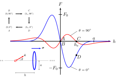
Figure 13: Force verses height $h$ for $\theta=0$ and $\theta=90^{\circ}$. States $A$, $B$, $C$, and $D$, for the Casimir machine are marked.

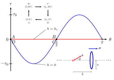
Figure 14: Torque verses orientation $\theta$ for $h=0$ and $h=h_{e}$. States $A$, $B$, $C$, and $D$, for the Casimir machine are marked.

Let us now examine the following mechanism. Consider an initial configuration $(h=0,\theta=0)$ denoted by state ‘A’ in Figs. 12 to 14. We assume that the atom can manipulate the orientation $\theta$ from $0^{\circ}$ to $90^{\circ}$ at the expense of internal energy. The new state $(h=0,\theta=90^{\circ})$ is denoted by state ‘B’ in Figs. 12 to 14. This will propel the ring away due to repulsion, leading to the configuration $(h=h_{e},\theta=90^{\circ})$ denoted by state ‘C’ in Figs. 12 to 14. The atom at this position manipulates the orientation $\theta$ from $90^{\circ}$ to $0^{\circ}$ at the expense of no internal energy, see discussion after Eq. (88). The new state $(h=h_{e},\theta=0^{\circ})$ is denoted by state ‘D’ in Figs. 12 to 14. This will propel the ring closer to the atom due to attraction. The cycle $A\to B\to C\to D\to A$, see Fig. 15, thus is a machine that is able to control the position of the ring at the expense of internal energy in the step $A\to B$.

Figure 15: Configuration states in the Casimir machine in Figs. 12 to 14.

The change in energies in the individual steps in the cycle are the following:

$$W_{A\to B} = -\int_{0,h=0}^{\frac{\pi}{2}}\tau d\theta=E(0,\frac{\pi}{2})-E(0,0)>0,$$ (151a)

$$W_{B\to C} = -\int_{0,\theta=\frac{\pi}{2}}^{h_{e}}Fdh=E(h_{e},\frac{\pi}{2})-E(0,\frac{\pi}{2})<0,\hskip 28.45274pt$$ (151b)

$$W_{C\to D} = -\int_{0,h=h_{e}}^{\frac{\pi}{2}}\tau d\theta=E(h_{e},0)-E(h_{e},\frac{\pi}{2})=0,$$ (151c)

$$W_{D\to A} = -\int_{h_{e},\theta=0}^{0}Fdh=E(0,0)-E(h_{e},0)<0,$$ (151d)

where the energies are evaluated using Eq. (146). As noted, the energy input is in $A\to B$. The step from $C\to D$ is achieved at no cost in internal energy.

IX Conclusion and outlook

We have derived and presented Casimir-Polder interaction energies between an anisotropically polarizable atom and an anisotropically polarizable ring, and when ring is replaced with an annular disc. Then, taking the outer radius to infinity to obtain a plate with circular aperture. We have identified specific configurations that lead to repulsive Casimir-Polder forces on the atom. We observe that when the relative orientations of the polarizabilities of the atom and the ring are perpendicular to each other the atom experiences a repulsive force when it is very close to the center of the ring. The energy-distance plots in Figs. 3, 7, and 9, mimics the energy-distance plot for an elongated needle shaped conductor and a plate with an aperture in Ref. Levin et al. (2010). These plots also have the qualitative features of the energy-distance plot reported for an atom and a conducting toroid in Ref. Abrantes et al. (2018). As suspected early on, these interaction energies seem to be characterized by the interaction of the individual eigenbasis of anisotropic polarizabilities of the objects. These dyadic-dyadic interactions are very rich due to the various possible interactions between the principal polarizations. To illustrate this richness, we have shown that in our energy-distance plots for an atom and ring, in addition to repulsion at short distances when the orientations are relatively perpendicular, we find another region of repulsion at intermediate distances when the orientations are relatively almost parallel.

We recognize that experimental observation of repulsion resulting from anisotropy and perforated geometries is lacking because the force is extremely weak. Numerical estimate of these energies is of the order of $\mu$eV, which is small. However, the energies between conducting bodies in contrast to dielectric materials considered in this article is expected to be larger Venkataram et al. (2020). We also note that non-monotonic Casimir forces in the context of two interlocked corrugated geometries resembling a ‘zipper’ were proposed in Ref. Rodriguez et al. (2008), which has now been realized experimentally Tang et al. (2017). These developments are expected to play an important role in the advancement of nanoscale machines.

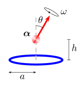
Figure 16: A spinning anisotropically polarizable atom of polarizability ${\bm{\alpha}}$ at a height $h$ above a dielectric ring of radius $a$. The atom is spinning with angular speed $\omega$ about the direction of polarization while maintaining an angle $\theta$ with the axis of the ring.

We confined our discussion here to static configurations. This prompts the question of whether stable equilibrium can be achieved in these configurations when the interactions are induced by quantum vacuum fluctuations? By generalizing Earnshaw’s theorem to include fluctuation-induced forces, the authors of Ref. Rahi et al. (2010) conclude that neutral polarizable objects cannot be in stable equilibrium in the quantum vacuum. However, like in electrostatics, it might still be possible to have stable equilibrium in dynamical configurations. We intend to study if a spinning polarizable atom, as described in Fig. 16, will precess and in the process attain dynamical stable equilibrium. This would be a Casimir-Polder analog of the Levitron${}^{\text{TM}}$ Berry (1996).