On Random Matrices Arising
in Deep Neural Networks: General I.I.D. Case

Abstract

We study the eigenvalue distribution of random matrices pertinent to the analysis of deep neural networks. The matrices resemble the product of the sample covariance matrices, however, an important difference is that the analog of the population covariance matrix is now a function of random data matrices (synaptic weight matrices in the deep neural network terminology). The problem has been treated in recent work [1] by using the techniques of free probability theory. Since, however, free probability theory deals with population covariance matrices which are independent of the data matrices, its applicability in this case has to be justified. The justification has been given in [2] for Gaussian data matrices with independent entries, a standard analytical model of free probability, by using a version of the techniques of random matrix theory. In this paper we use another version of the techniques to extend the results of [2] to the case where the entries of the data matrices are just independent identically distributed random variables with zero mean and finite fourth moment. This, in particular, justifies the mean field approximation in the infinite width limit for the deep untrained neural networks and the property of the macroscopic universality of random matrix theory in this case.

1 Introduction

Deep learning, a powerful computational technique based on deep artificial neural networks (DNN) of various architecture, proved to be an efficient tool in a wide variety of problems involving large data sets, see, e.g. [4, 5, 6, 7, 8, 9]. A general scheme for the so-called feed-forward, fully connected neural networks with $L$ layers of width $n_{l}$ for the $l$th layer is as follows.

Let

$$x^{0}=\{x_{j_{0}}^{0}\}_{j_{0}=1}^{n_{0}}\in\mathbb{R}^{n_{0}}$$ (1.1)

be the input to the network and $x^{L}=\{x_{j_{L}}^{L}\}_{j_{L}=1}^{n_{L}}\in\mathbb{R}^{n_{L}}$ be the output. Their components are known as the neurons (the terminology here and below is inspired by that in biological neural networks). The components of the activations $x^{l}=\{x_{j_{l}}^{l}\}_{j_{l}=1}^{n_{l}},\;l=1,\dots,L-1$ and the components of the post-affine transformations $y^{l}=\{y_{j_{l}}^{l}\}_{j_{l}=1}^{n_{l}}$ in the $l$th layer are related via an affine transformation

$$y^{l}=W^{l}x^{l-1}+b^{l},\;x_{j_{l}}^{l}=\varphi(y_{j_{l}}^{l}),\;j_{l}=1,\dots,n_{l},\;l=1,\dots,L,$$ (1.2)

where

$$W^{l}=\{W_{j_{l}j_{l-1}}^{l}\}_{j_{l},j_{l-1}=1}^{n_{l},n_{l-1}},\;l=1,\dots,L$$ (1.3)

are $n_{l}\times n_{l-1}$ weight matrices,

$$b^{l}=\{b_{j_{l}}^{l}\}_{j_{l}=1}^{n_{l}},\;l=1,\dots,L$$ (1.4)

are $n_{l}$-component bias vectors and $\varphi:\mathbb{R}\rightarrow\mathbb{R}_{+}$ is the component-wise nonlinearity known as the activation function. It is usually monotone and piece-wise differentiable (S-shaped or sigmoid), e.g. $tanh$, $tan^{-1}$, $(1+e^{-x})^{-1}$ and HardTanh (see (2.54)). A widely used and fast calculated activation function is the rectified linear unit (ReLU) $x_{+}:=\max\{0,x\}$.

An important ingredient of the deep learning is the training procedure. It modifies the parameters (weight matrices and biases) on the every step of the iteration to reduce the misfit between the input and the output data of the layer by using certain optimization procedures, usually the stochastic gradient descend (SGD). Being multiply repeated in the DNN, the procedure provides the desired final output as well as certain final parameters of the DNN in question.

In the DNN practice the weights and the biases are randomly initialized and the SGD also includes a certain randomization. Moreover, the modern theory deals also with untrained and even random parameters of the DNN architecture, see [1, 3, 8, 11, 12, 13, 14, 15, 16, 17, 18, 19, 21, 20]. It is often assumed in these and other works that the weight matrices and biases are independent and identically distributed (i.i.d.) in $l$ and have i.i.d. Gaussian entries and components.

Following this trend in the DNN studies and taking into account that quite common initialization schemes in deep learning do not use Gaussians [25] on one hand and recalling the independence of various results of random matrix theory on the concrete distribution of the parameters (macroscopic universality) [22, 23] on the other hand, we consider in this paper a general i.i.d. case where:

(i) the bias vectors $b^{l},\;l=1,2,\dots,L$ are i.i.d. in $l$ and for every $l$ their components $\{b_{j_{l}}^{l}\}_{j_{l}=1}^{n_{l}}$ are i.i.d. random variables such that

$$\mathbf{E}\{b_{j_{l}}^{l}\}=0,\;\mathbf{E}\{(b_{j_{l}}^{l})^{2}\}=\sigma_{b}^{2},$$ (1.5)

(ii) the weight matrices $W^{l},\;l=1,2\dots,L$ are also i.i.d in $l$ and

$$W^{l} =n_{l-1}^{-1/2}X^{l}=n_{l-1}^{-1/2}\{X_{j_{l}j_{l-1}}^{l}\}_{j_{l},j_{l-1}=1}^{n_{l},n_{l-1}},$$

$$\mathbf{E}\{X_{j_{l}j_{l-1}}^{l}\} =0,\;\mathbf{E}\{(X_{j_{l}j_{l_{1}-1}}^{l})^{2}\}=w^{2},\;\mathbf{E}\{(X_{j_{l}j_{l_{1}-1}}^{l})^{4}\}=m_{4}<\infty,$$ (1.6)

where for every $l$ the entries $\{X_{j_{l}j_{l-1}}^{l}\}_{j_{l},j_{l-1}=1}^{n_{l},n_{l-1}}$ of $X^{l}$ are i.i.d. random variables.

Note that the quite common initialization schemes in deep learning do not use Gaussians, see, e.g. [25].

We will view $n_{l}\times n_{l-1}$ matrices $X^{l}$ as the upper left rectangular blocks of the semi-infinite random matrix

$$\{X_{j_{l}j_{l-1}}^{l}\}_{j_{l},j_{l-1}=1}^{\infty,\infty}$$ (1.7)

whose i.i.d. entries satisfy (1.6).

Likewise, for every $l$ we will view $b^{l}$ in (1.4) as the first $n_{l}$ components of the semi-infinite vector

$$\{b_{j_{l}}^{l}\}_{j_{l}=1}^{\infty}$$ (1.8)

whose i.i.d. components satisfy (1.5).

As a result of this form of weights and biases of the $l$th layer they are for all $n_{l}=1,2,\dots$ defined on the same infinite-dimensional product probability space $\Omega^{l}$ generated by (1.7) – (1.8). Let also

$$\Omega_{l}=\Omega^{l}\times\Omega^{l-1}\times\dots\times\Omega^{1},\;l=1,\dots,L$$ (1.9)

be the infinite-dimensional probability space on which the recurrence (1.2) is defined for a given $L$ (the number of layers).

This procedure of enlarging the probability space is standard in probability theory, see e.g. [37]. In our case the procedure allows us to formulate our results on the large size asymptotic behavior of the eigenvalue distribution of matrices (1.12) as those valid with probability 1 in $\Omega_{L}$, i.e., for any "typical" realization of random parameters (for an analogous approach in random matrix theory see, e.g. [22])."

A key and quite non-trivial step in training deep networks is to move the weights $W^{l}$, hence, the activations $x^{l}$ in each layer $l$ so as to move the output $x^{L}$ in the final layer in a desired direction. To this end the analysis of the back propagation of errors at the output of layer $l$, determining how we have to change $x^{l}$ to move $x^{L}$, is useful. A corresponding tool is the Jacobian $\frac{\partial x^{L}}{\partial x^{0}}$ showing how an error $\varepsilon$, or desired direction of motion in the output $x^{L}$, back-propagates to a desired change in the input $\Delta(x^{0})^{T}=\varepsilon^{T}J$, see more in [3, 18].

The above makes the Jacobian an important quantity of the field. We have according to (1.1) – (1.4)

$$J_{\mathbf{n}_{L}}^{L}:=\left\{\frac{\partial x_{j_{L}}^{L}}{\partial x_{j_{0}}^{0}}\right\}_{j_{0},j_{L}=1}^{n_{0},n_{L}}=D^{L}W^{L}\cdots D^{1}W^{1},\;\mathbf{n}_{L}=(n_{1},\dots,n_{L}),$$ (1.10)

an $n_{L}\times n_{0}$ random matrix, where $\{W^{l}\}_{l=1}^{L}$ are given by (1.6) and

$$D^{l}=\{D_{j_{l}}^{l}\delta_{j_{l}k_{l}}\}_{j_{l},k_{l}=1}^{n_{l}},\;D_{j_{l}}^{l}=\varphi^{\prime}\Big{(}n_{l-1}^{-1/2}\sum_{j_{l-1}=1}^{n_{l-1}}X_{j_{l}j_{l-1}}^{l}x_{j_{l-1}}^{l-1}+b_{j_{l}}^{l}\Big{)},\;l=1,\dots,L$$ (1.11)

are diagonal random matrices.

Of particular interest is the spectrum of singular values of $J_{\mathbf{n}_{L}}^{L}$, i.e., the square roots of eigenvalues of the $n_{L}\times n_{L}$ positive definite matrix

$$M_{\mathbf{n}_{L}}^{L}=J_{\mathbf{n}_{L}}^{L}(J_{\mathbf{n}_{L}}^{L})^{T}$$ (1.12)

for networks with the above random weights and biases and for large $\{n_{l}\}_{l=1}^{L}$, i.e., for deep networks with wide layers but with a fixed depth $L$, see [1, 13, 14, 15, 16, 18, 19, 20] for motivations, settings and results. More precisely, we will study in this paper the asymptotic regime determined by the simultaneous limits

$$n_{l}\rightarrow\infty,\;n_{l-1}/n_{l}\to c_{l}\in(0,\infty),\;\;l=1,\dots,L$$ (1.13)

denoted below as

$$\lim_{\mathbf{n}_{L}\rightarrow\infty}\dots$$ (1.14)

The above limit can be viewed as an implementation of the heuristic inequality $L\ll n$, meaning that the DNN in question are much more wide than they are deep. The simplest case where $L=1$ and $D_{1}=\mathbf{1}_{n}$ is known in statistics as the Wishart matrices [22, 24] and in this case the limiting NCM (see (1.16) for definition) is

$$\nu_{MP}(\lambda)=(2\pi)^{-1}\sqrt{(4-\lambda)/\lambda},\;\lambda\in[1,4].$$ (1.15)

Denote by $\{\lambda_{t}^{L}\}_{t=1}^{n_{L}}$ the eigenvalues of the real symmetric random matrix (1.12) and introduce its Normalized Counting Measure (NCM)

$$\nu_{M_{\mathbf{n}_{L}}^{L}}=n_{L}^{-1}\sum_{t=1}^{N_{L}}\delta_{\lambda_{t}^{L}}.$$ (1.16)

We will deal with the leading term of $\nu_{M_{\mathbf{n}_{L}}^{L}}$in the asymptotic regime (1.13), i.e., with the limit

$$\nu_{M^{L}}=\lim_{\mathbf{n}_{L}\rightarrow\infty}\nu_{M_{\mathbf{n}_{L}}^{L}}.$$ (1.17)

Note that since $\nu_{M_{\mathbf{n}_{L}}^{L}}$ is random, the meaning of the limit has to be indicated.

The problem has been considered in [1] (see also [2, 3, 13, 19, 20]) in the case where all $b^{l}$ and $X^{l},\;l=1,2,\dots,L$ in (1.5) – (1.6) are Gaussian and have the same size $n$ and $n\times n$ respectively, i.e.,

$$n=n_{0}=\dots=n_{L},\;c_{l}=1,\;l=1,\dots,L.$$ (1.18)

In [1] compact formulas for the limit

$$\overline{\nu}_{M^{L}}=\lim_{n\rightarrow\infty}\overline{\nu}_{M_{n}^{L}},\;\overline{\nu}_{M_{n}^{L}}:=\mathbf{E}\{\nu_{M_{n}^{L}}\}$$ (1.19)

and its Stieltjes transform

$$f_{M^{L}}(z)=\int_{0}^{\infty}\frac{\overline{\nu}_{M^{L}}(d\lambda)}{\lambda-z},\;\Im z\neq 0$$ (1.20)

were presented. The formula for $\overline{\nu}_{M^{L}}$ is given in (2.30) below. To write the formula for $f_{M^{L}}$ it is convenient to use the moment generating function

$$m_{M^{L}}(z)=\sum_{k=1}^{\infty}m_{k}z^{k},\;m_{k}=\int_{0}^{\infty}\lambda^{k}\overline{\nu}_{M^{L}}(d\lambda),$$ (1.21)

of $\overline{\nu}_{M^{L}}$ related to $f_{M^{L}}$ as

$$m_{M^{L}}(z)=-1-z^{-1}f_{M^{L}}(z^{-1}).$$ (1.22)

Let

$$K_{n}^{l}:=(D_{n}^{l})^{2}=\{(D_{j_{l}}^{l})^{2}\}_{j_{l}=1}^{n}$$ (1.23)

be the square of the $n\times n$ random diagonal matrix (1.11) with $n_{l}=n$ and let $m_{K^{l}}$ be the moment generating function of the $n\rightarrow\infty$ limit $\overline{\nu}_{K^{l}}$ of the expectation of the NCM of $K_{n}^{l}$. Then we have according to formulas (14) and (16) in [1] in the case, where $\overline{\nu}_{K^{l}}$, hence $m_{K^{l}}$, do not depend on $l$ (see Remark 2.6 (i)),

$$m_{M^{L}}(z) =m_{K}(z^{1/L}\psi_{L}(m_{M^{L}}(z)),$$

$$\psi_{L}(m) =m^{(L-1)/L}(1+m)^{1/L}.$$ (1.24)

Hence, $f_{M^{L}}$ of (1.20) satisfies a certain functional equation, the standard situation in random matrix theory and its applications, see [22] for general results and [26, 27] for results on the products of random matrices. Note that our notation is different from that of [1]: our $f_{M^{L}}(z)$ of (1.20) is $-G_{X}(z)$ of (7) in [1] and our $m_{M^{L}}(z)$ of (1.21) is $M^{-1}_{X}(1/z)$ of (9) in [1].

The derivation of (1.24) and the corresponding formulas (see (2.30) – (2.34) below) for the limiting mean NCM $\overline{\nu}_{M^{L}}$ in [1] are based on the claimed in this paper asymptotic freeness of diagonal matrices $D_{n_{l}}^{l}=\{D_{j_{l}}^{l}\}_{j_{l}=1}^{n_{l}},\;l=1,\dots,L$ of (1.11) and Gaussian matrices $X_{n_{l}}^{l},\;l=1,\dots,L$ of (1.3) – (1.6) (see, e.g. [28] for the definitions and properties of asymptotic freeness). This leads directly to (1.24) in view of the multiplicative property of the moment generating functions (1.21) and the so-called $S$-transforms of the mean limiting NCM $\overline{\nu}_{K^{l}}$ of $K_{n_{l}}^{l}$ and the mean limiting NCM $\overline{\nu}_{MP}$ (see (1.15)) of $n^{-1}X_{n_{l}}^{l}(X_{n_{l}}^{l})^{T}$ in the regime (1.13), see Remark 2.6 (ii) and Corollary 2.3.

There is, however, a delicate point in the argument of [1], since, to the best of our knowledge, the asymptotic freeness has been established so far for the Gaussian random matrices $X_{n_{l}}^{l}$ of (1.6) and deterministic (more generally, random but $X_{n_{l}}^{l}$-independent) diagonal matrices, see e.g. [28] and also [26, 27]. On the other hand, the diagonal matrices $D_{n}^{l}$ in (1.11) depend explicitly on $(X_{n}^{l},b_{n}^{l})$ of (1.3) – (1.4) and, implicitly, via $x^{l-1}$, on the all preceding $(X_{n}^{l^{\prime}},b_{n}^{l^{\prime}}),\;l^{\prime}=l-1,\dots,1$. Thus, the proof of validity of (1.24) requires an additional reasoning.  It was given in [2] for the Gaussian weights and biases by using a version of standard tools of random matrix theory (see [22], Chapter 7). Note that it was also proved in [2] that the formula (1.17) is valid not only in the mean (see (1.19) and [1]), but also with probability 1 in $\Omega_{L}$ of (1.9) (recall that the measures in the r.h.s. of (1.17) are random) and that the corresponding limiting measure $\nu_{M^{L}}$ coincides with $\overline{\nu}_{M^{L}}$ of (1.19), i.e., $\nu_{M^{L}}$ is non-random (the selfaveraging property of the limiting NCM).

The basic ingredient of the proof in [2] is the justification of the replacement of the argument of $\varphi^{\prime}$ in (1.11), i.e., the post-affine $y_{j_{l}}^{l}$ of (1.2), by a Gaussian random variable which is statistically independent of $\{X^{l^{\prime}}\}_{l^{\prime}=1}^{l}$, see Lemma 3.5 of [2]. This reduces the analysis of random matrices (1.12) to that of random matrices with random but $X^{l}$-independent analogs of diagonal matrices $D^{l}$, a well studied problem of random matrix theory, see, e.g. [2, 29], and justifies the so-called infinite width mean-field limit discussed in [14, 16, 18, 20].

The goal of this paper is to show that the results presented in [1] and justified in [2] (see also [20]) for the Gaussian weights and biases are valid for arbitrary random weights and biases satisfying (1.5) – (1.6). It is worth mentioning that our initial intention was to carry out this extension just by using the so-called interpolation trick of random matrix theory. The trick allows one to extend a number of results of the theory valid for Gaussian matrices with i.i.d. entries to those for matrices with i.i.d. entries possessing just several finite moments, see [22, 30] (this is known as the macroscopic, or global, universality). We have found, however, that in our case the corresponding proof is quite tedious and long. Thus, we apply another method which dates back to [31, 32] and has been widely used and extended afterwards [22, 33, 34, 35]. The method is quite transparent and its application to matrices (1.12) requires just minor modifications of that used in random matrix theory where the analogs of matrices $D^{l}$ of (1.11) are either non-random or random but independent of $X^{l}$ of (1.6).

The paper is organized as follows. In the next Section 2 we prove the validity of (1.17) with probability 1 in $\Omega_{L}$ of (1.9), formula (1.24) and the corresponding formula (2.30) for $\nu_{M^{L}}=\overline{\nu}_{M^{L}}$ of [1]. This is given in Theorem 2.5 which proof is based on a natural inductive procedure allowing for the passage from the $l$th to the $(l+1)$th layer and it is quite close to that of [2]. This is because the procedure is almost independent on the probability law of the weight entries, provided that a formula relating the limiting (in the layer width) Stieltjes transforms of the NCMs of two subsequent layers is known for these entries. For the i.i.d. case of the present paper the formula is the same as that in [1, 2] for the Gaussian case, although its proof is quite different from that in [2]. The formula is given in Theorem 2.1. Section 2 includes also certain numerical results that illustrate and confirm our analytical results. Section 3 contains the proof of Theorem 2.1 as well as necessary auxiliary results used in the proof.

Note that to make the paper self-consistent we present here certain facts that have been already given in our previous paper [2].

2 Main Result and its Proof.

As was already mentioned in Introduction, the goal of the paper is to extend the results presented in [1] and justified in [2] for Gaussian weights and biases to those satisfying (1.5) – (1.6) but not necessarily Gaussian. We will prove that in this fairly general case the resulting eigenvalue distribution of random matrices (1.12) coincides with that of matrices of the same form where, however, the analogs of diagonal matrices (1.11), (1.23) are random but independent of $X^{l}$ (see Theorem 2.5, formulas (2.31) – (2.32) in particular). Thus, we will comment first on the corresponding result of random matrix theory (see, e.g. [2, 22, 29] and references therein).

Consider for every positive integer $n$: (i) the $n\times n$ random matrix $X_{n}$ with i.i.d. entries satisfying (1.6); (ii) positive definite matrices $\mathsf{K}_{n}$ and $\mathsf{R}_{n}$ that are either deterministic or even random but independent of $X_{n}$ and such that their Normalized Counting Measures $\nu_{\mathsf{K}_{n}}$ and $\nu_{\mathsf{R}_{n}}$ (see (1.16)) converge weakly as $n\rightarrow\infty$ (with probability 1 if random in an appropriate probability space $\Omega_{\mathsf{KR}}$) to non-random measures $\nu_{\mathsf{K}}$ and $\nu_{\mathsf{R}}$. Set

$$\mathsf{M}_{n}=n^{-1}\mathsf{K}_{n}^{1/2}X_{n}\mathsf{R}_{n}X_{n}^{T}\mathsf{K}_{n}^{1/2}.$$ (2.1)

According to random matrix theory (see, e.g. [2, 22, 29] and references therein), in this case and under certain conditions on $X_{n}$ the Normalized Counting Measure $\nu_{\mathsf{M}_{n}}$ of $\mathsf{M}_{n}$ converges weakly with probability 1 as $n\rightarrow\infty$ (in the probability space $\Omega_{\mathsf{KR}}\times\Omega_{X}$, cf. (1.7)) to a non-random measure $\nu_{\mathsf{M}}$ which is uniquely determined by the limiting measures $\nu_{\mathsf{K}}$ and $\nu_{\mathsf{R}}$ via a certain analytical procedure. We can write down this fact symbolically as

$$\nu_{\mathsf{M}}=\nu_{\mathsf{K}}\diamond\nu_{\mathsf{R}}.$$ (2.2)

In fact, the procedure defines a binary operation in the set of non-negative measures with the total mass 1 and a support belonging to the positive semi-axis (see more in Corollary 2.3).

The main result of works [1, 2, 20], dealing with Gaussian weights and biases and extended in this paper for any i.i.d. weights and biases satisfying (1.6) and (1.5)), is that the limiting Normalized Counting Measure (1.17) of random matrices (1.12), where the role of $\mathsf{K}_{n}$ of (2.1) plays the matrix defined by (1.11) and (1.23) and depending on matrices $\{X^{l}\}^{L}_{l=1}$ of (1.6), is, nevertheless, equal to the "product" with respect the operation (2.2) of $L$ measures $\nu_{K^{l}},\;l=1,...,L$ that are the limiting Normalized Counting Measures of random matrices of (1.11) and (1.23).

Note that the operation (2.2) is closely related to the so-called multiplicative convolution of free probability theory [28], having the above random matrices as a basic analytic model.

Thus we will begin with a proof of this assertion which, we believe, is of independent interest for random matrix theory.

We follow [1, 2] and confine ourselves to the case (1.18) where all the weight matrices and bias vectors are of the same size $n$, see (1.18). The general case is essentially the same (see, e.g. Remark 2.2 (ii)).

In addition, we assume for the sake of simplicity of subsequent formulas that

$$w^{2}=1$$ (2.3)

in (1.6), thus, fixing the scale of the spectral axis. The general case follows from the above by a simple change of variables.

Theorem 2.1

Consider for every positive integer $n$ the $n\times n$ random matrix

$$\mathcal{M}_{n}=n^{-1}S_{n}X_{n}^{T}K_{n}X_{n}S_{n},$$ (2.4)

where:

(a) $S_{n}$ is a positive definite $n\times n$ matrix such that

$$\sup_{n}n^{-1}\mathrm{Tr}R_{n}^{2}=r_{2}<\infty,\;R_{n}=S_{n}^{2},$$ (2.5)

and

$$\lim_{n\rightarrow\infty}\nu_{R_{n}}=\nu_{R},\;\nu_{R}(\mathbb{R}_{+})=1,$$ (2.6)

where $\nu_{R_{n}}$ is the Normalized Counting Measure of $R_{n}$, $\nu_{R}$ is a non-negative measure not concentrated at zero and $\lim_{n\rightarrow\infty}$ denotes the weak convergence of probability measures (see [37], Section III.1);

(b) $X_{n}$ is the $n\times n$ random matrix

$$X_{n}=\{X_{j\alpha}\}_{j,\alpha=1}^{n},\;\mathbf{E}\{X_{j\alpha}\}=0,\;\mathbf{E}\{X_{j\alpha}^{2}\}=1,\;\mathbf{E}\{X_{j\alpha}^{4}\}=m_{4}<\infty$$ (2.7)

with jointly i.i.d. entries (cf. (1.6)), $b_{n}$ is the $n$-component random vector

$$b^{(n)}=\{b_{j}\}_{j=1}^{n},\;\mathbf{E}\{b_{j}\}=0,\;\mathbf{E}\{b_{j}^{2}\}=\sigma_{b}^{2}$$ (2.8)

with jointly i.i.d. components (cf. (1.5)) and for all $n$ the matrix $X_{n}$ and the vector $b_{n}$ viewed as defined on the same probability space

$$\Omega_{X,b}=\Omega_{X}\times\Omega_{b},$$ (2.9)

where $\Omega_{X}$ and $\Omega_{b}$ are generated by the analogs of (1.7) and (1.8);

(c) $K_{n}$ is the diagonal random matrix

$$K_{n}=\{\delta_{jk}K_{jn}\}_{j,k=1}^{n},\;K_{jn}=\left(\varphi^{\prime}\Big{(}n^{-1/2}\sum_{a=1}^{n}X_{j\alpha}x_{\alpha n}+b_{j}\Big{)}\right)^{2},$$ (2.10)

where $\varphi:\mathbb{R}\rightarrow\mathbb{R}$ is continuously differentiable, is not identically constant and such that (cf. (2.28))

$$\sup_{x\in\mathbb{R}}|\varphi(x)|=\Phi_{0}<\infty,\;\sup_{x\in\mathbb{R}}|\varphi^{\prime}(x)|=\Phi_{1}<\infty,$$ (2.11)

$x_{n}=\{x_{\alpha n}\}_{\alpha=1}^{n}$ is a collection of real numbers such that there exists the limit

$$q=\lim_{n\rightarrow\infty}q_{n}>\sigma_{b}^{2}>0,\;q_{n}=n^{-1}\sum_{\alpha=1}^{n}(x_{\alpha n})^{2}+\sigma_{b}^{2}$$ (2.12)

and

$$\lim_{n\rightarrow\infty}n^{-2}\sum_{\alpha=1}^{n}(x_{\alpha n})^{4}=0.$$ (2.13)

Then the Normalized Counting Measure (NCM) $\nu_{\mathcal{M}_{n}}$ of $\mathcal{M}_{n}$ converges weakly with probability 1 in $\Omega_{X,b}$ of (2.9) to a non-random measure $\nu_{\mathcal{M}}$, such that

$$\nu_{\mathcal{M}}(\mathbb{R_{+}})=1,$$ (2.14)

and that its Stieltjes transform $f_{\mathcal{M}}$ can be obtained from the formulas

$$f_{\mathcal{M}}(z): =\int_{0}^{\infty}\frac{\nu_{\mathcal{M}}(d\lambda)}{\lambda-z}$$

$$=\int_{0}^{\infty}\frac{\nu_{R}(d\lambda)}{k(z)\lambda-z}=-z^{-1}+z^{-1}h(z)k(z),\;z\in\mathbb{C}\setminus\mathbb{R}_{+},$$ (2.15)

where the pair ($h,k$) is the unique solution of the system of functional equations

$$h(z)=\int_{0}^{\infty}\frac{\lambda\nu_{R}(d\lambda)}{k(z)\lambda-z},\;z\in\mathbb{C}\setminus\mathbb{R}_{+}$$ (2.16)

$$k(z)=\int_{0}^{\infty}\frac{\lambda\nu_{K}(d\lambda)}{h(z)\lambda+1},\;z\in\mathbb{C}\setminus\mathbb{R}_{+},$$ (2.17)

in which $\nu_{R}$ is defined in (2.6), and

$$\nu_{K}(\Delta)=\mathbf{P}\Big{\{}\big{(}\varphi^{\prime}((q-\sigma_{b}^{2})^{1/2}\gamma+b_{1})\big{)}^{2}\in\Delta\Big{\}},\;\Delta\in\mathbb{R},$$ (2.18)

where $q$ is given by (2.12), $\gamma$ is the standard Gaussian random variable and we are looking for a solution of (2.16) – (2.17) in the class of pairs $(h,k)$ of functions analytic outside the closed positive semi-axis, continuous and positive on the negative semi-axis and such that

$$\Im h(z)\Im z>0,\;\Im z\neq 0;\;\sup_{\xi\geq 1}\xi h(-\xi)\in(0,\infty).$$ (2.19)

The proof of the theorem is given in the next section. Here are the remarks.

Remark 2.2

(i) To apply Theorem 2.1 to the proof of Theorem 2.5 we need a version of the former in which its "parameters", i.e., $R_{n}$, hence $S_{n}$, in (2.4) – (2.6) and (possibly) $\{x_{\alpha n}\}_{\alpha=1}^{n}$ in (2.10) are random, defined for all $n$ on the same probability space $\Omega_{R,x}$, independent of $\Omega_{X,b}$ of (2.9) and satisfy conditions (2.5) – (2.6) and (2.12) – (2.13) with probability 1 in $\Omega_{R,x}$, i.e., on a certain subspace (cf. (2.37))

$$\overline{\Omega}_{R,x}\subset\Omega_{R,x},\;\mathbf{P}(\overline{\Omega_{R,x}})=1.$$ (2.20)

In this case Theorem 2.1 is valid with probability 1 in $\Omega_{X,b}\times\Omega_{R,x}$. The corresponding argument is standard in random matrix theory, see, e.g. Section 2.3 of [22] and Remark 2.6 (iii). The obtained limiting NCM $\nu_{\mathcal{M}}$ is random in general due to the (possible) randomness of $\nu_{R}$ and $q$ in (2.6) and (2.12) which are defined on their "own" probability space $\Omega_{R,x}$ distinct from $\Omega_{X,b}$. Note, however, that in the case of Theorem 2.5 the corresponding analogs of $\nu_{R}$ and $q$ are not random, thus the limiting measure $\nu_{M^{L}}$ is non-random as well.

(ii) Repeating almost literally the proof of the theorem, one can treat a more general case where $S_{m}$ is $m\times m$ positive definite matrix satisfying (2.5) – (2.6), $K_{n}$ is the $n\times n$ diagonal matrix given by (2.10) – (2.12), $X_{n}$ is a $n\times m$ random matrix satisfying (1.6) and (cf. (1.13))

$$\lim_{m\rightarrow\infty,n\rightarrow\infty}m/n=c\in(0,\infty).$$

In this case the Stieltjes transform $f_{\mathcal{M}}$ of the limiting NCM is again uniquely determined by three formulas where the first and the second are (2.15) and (2.16) with $k(z)$ replaced by $k(z)c^{-1}$ and the third coincides with (2.17).

(iii) Theorem 2.1 is proved above for bounded $\varphi$ and $\varphi^{\prime}$ (see (2.10) and (2.11)) and for the entries of $X_{n}$ and the components of $b$ having the finite fourth and the second moment respectively (see (2.7) – (2.8). However, assuming the finiteness of these moments of sufficiently large order, it is possible to extend the theorem to the case where $\varphi$ and $\varphi^{\prime}$ are just polynomially bounded. It suffices to apply to the matrices $K_{n}^{l}$ of (2.10) a truncation procedure similar to that used for the matrix $R_{n}$ of (2.5), see formula (3.52) and the subsequent text. Correspondingly, Theorem 2.5 can also be extended similarly, however in this case the maximal order of finite moments depends on $L$.

(iv) The theorem provides the justification of the statistical independence of the random argument $n^{-1/2}(X_{n}x_{n})_{j}+b_{j}$ of (2.10) and the weight matrix $n^{-1/2}X_{n}$ in (2.4) in the infinite width limit $n\to\infty$. The assumption has been used in a number of works (see e.g. [1, 14, 16, 15, 18]) and is known as the mean field approximation, since it has certain similarity to the mean field approximation in statistical mechanics and related fields.

Theorem 2.1 yields an explicit form of the binary operation (2.2) via equations (2.15) – (2.17). Following [2], it is convenient to write the equations in a compact form similar to that of free probability theory [28]. This, in particular, makes explicit the symmetry and the transitivity of the operation.

Corollary 2.3

Let $\nu_{K},\;\nu_{R}$ and $\nu_{\mathcal{M}}$ be the probability measures (non-negative measures of the total mass 1) entering (2.15) – (2.17) and $m_{K},\;m_{R}$ and $m_{\mathcal{M}}$ be their moment generating functions (see (1.21) – (1.22)). Then their functional inverses $z_{K},\;z_{R}$ and $z_{\mathcal{M}}$ are related as follows

$$z_{\mathcal{M}}(m)=z_{K}(m)z_{R}(m)m^{-1},$$ (2.21)

or, writing

$$z_{A}(m)=m\sigma_{A}(m),\;A=K,R,\mathcal{M,}$$ (2.22)

we obtain the simple "algebraic" form

$$\sigma_{\mathcal{M}}(m)=\sigma_{K}(m)\sigma_{R}(m)$$ (2.23)

of the operation $\diamond$ of (2.2).

Proof. It follows from (2.16) – (2.17) and (1.22) that

$$m_{K}(-h(z))=-h(z)k(z),\;m_{R}(k(z)z^{-1})=-h(z)k(z),$$

$$\hskip 28.45274ptm_{\mathcal{M}}(z^{-1})=-h(z)k(z).$$ (2.24)

Now the first and the third relations (2.24) yield $m_{K}(-h(z^{-1}))=m_{\mathcal{M}}(z)$, hence $z_{K}(m)=-h(z_{\mathcal{M}}^{-1}(m))$, and then the second and the third relations yield $m_{R}(k(z^{-1})z)=m_{\mathcal{M}}(z)$, hence $z_{R}(\mu)=k(z_{\mathcal{M}}^{-1}(m))z_{\mathcal{M}}(m)$. Multiplying these two relations and using once more the third relation in (2.24), we obtain

$$z_{K}(m)z_{R}(m)=-k(z_{\mathcal{M}}^{-1}(m))h(z_{\mathcal{M}}^{-1}(m))z_{\mathcal{M}}(m)=z_{\mathcal{M}}(m)m$$

and (2.21) – (2.23) follows.   

Remark 2.4

In the case of rectangular matrices $X_{n}$ in (2.4), described in Remark 2.2 (ii), the analogs of (2.21) and (2.23) are

$$z_{\mathcal{M}}(m)=z_{K}(cm)z_{R}(cm)m^{-1},\;\sigma_{\mathcal{M}}(m)=c^{2}\sigma_{K}(cm)\sigma_{R}(cm).$$ (2.25)

We will now formulate and prove our main result.

Theorem 2.5

Let $M_{n}^{L}$ be the random matrix (1.12) defined by (1.2) – (1.11) and (1.18), where the weights $\{W^{l}\}_{l=1}=\{n^{-1/2}X^{l}\}_{l=1}$ and biases $\{b^{l}\}_{l=1}$ are i.i.d. in $l$ with i.i.d. entries and components satisfying (1.5) – (1.6) and the input vector $x^{0}$ (1.1) (deterministic or random) is such that there exists a finite limit

$$q^{1}:=\lim_{n\rightarrow\infty}q_{n}^{1}>\sigma_{b}^{2}>0,\;\;q_{n}^{1}=n^{-1}\sum_{j_{0}=1}^{n}(x_{j_{0}}^{0})^{2}+\sigma_{b}^{2}$$ (2.26)

and

$$\lim_{n\rightarrow\infty}n^{-2}\sum_{j_{0}=1}^{n}(x_{j_{0}}^{0})^{4}=0.$$ (2.27)

Assume also that the activation function $\varphi$ in (1.2) is continuously differentiable, $\varphi^{\prime}$ is not zero identically and

$$\sup_{t\in\mathbb{R}}|\varphi(t)|=:\Phi_{0}<\infty,\;\sup_{t\in\mathbb{R}}|\varphi^{\prime}(t)|=:\Phi_{1}<\infty.\;\;$$ (2.28)

Then the Normalized Counting Measure (NCM) $\nu_{M_{n}^{L}}$ of $M_{n}^{L}$ (see (1.16)) converges weakly with probability 1 in the probability space $\Omega_{L}$ of (1.9) to a non-random limit

$$\nu_{M^{L}}=\lim_{n\to\infty}\nu_{M^{L}_{n}},$$ (2.29)

where

$$\nu_{M^{L}}=\nu_{K^{L}}\diamond\cdots\diamond\nu_{K^{1}},$$ (2.30)

the operation "$\diamond$" is defined in (2.2) (see also Remark 2.6 (ii) Corollary 2.3 below) and

$$\nu_{K^{l}}(\Delta)=\mathbf{P}\Big{\{}\big{(}\varphi^{\prime}((q^{l}-\sigma_{b}^{2})^{1/2}\gamma+b_{1})\big{)}^{2}\in\Delta\Big{\}},\;\Delta\in\mathbb{R},\;l=1,...,L,$$ (2.31)

with the standard Gaussian random variable $\gamma$ and $q^{l}$ determined by the recurrence

$$q^{l}=\int\varphi^{2}\Big{(}\gamma(q^{l-1}-\sigma_{b}^{2})^{1/2}+b\Big{)}\Gamma(d\gamma)F(db),\;l\geq 2,$$ (2.32)

where $\Gamma(d\gamma)=(2\pi)^{1/2}e^{-\gamma^{2}/2}d\gamma$ is the standard Gaussian measure, $F$ is the probability law of $b_{1}^{l}$ in (1.5) and $q^{1}$ is given by (2.26).

Remark 2.6

(i) If

$$q_{1}=\cdots=q_{L}=:q^{*},$$ (2.33)

then $\nu_{K}:=\nu_{K^{l}},\;l=1,\dots,L$ and (2.30) becomes

$$\nu_{M^{L}}=\underset{L\;\mathrm{times}}{\underbrace{\nu_{K}\diamond\nu_{K}\cdots\diamond\nu_{K}}}.$$ (2.34)

Equalities (2.33) are the case if $q^{\ast}$ is a fixed point of (2.32), see [14, 16, 18] for a detailed analysis of (2.32) with Gaussian $F$ and its role in the functioning of the deep neural networks.

(ii) Let us show that Theorem 2.5 implies the results of [1], formula (1.24) in particular. Indeed, it follows from the theorem, (2.48), and Corollary 2.3 that the functional inverse $z_{M^{l+1}}$ of the moment generating function $m_{M^{l+1}}$ (see (1.21) – (1.22)) of the limiting NCM $\nu_{M^{l+1}}$ of matrix $M_{n}^{l+1}$ and that of $M_{n}^{l}$ are related as (cf. (2.21))

$$z_{M^{l+1}}(m)=z_{K^{l+1}}(m)z_{M^{l}}(m)m^{-1}.$$ (2.35)

Passing from the moment generating functions to the S-transforms of free probability theory via the formula $S(m)=z(m)(1+m)m^{-1}$ [28] and taking into account that for the limiting NCM (1.15) of the Wishart matrix $n^{-1}X_{n}X_{n}^{T}$, we have $z_{MP}(m)=m(1+m)^{-2}$ and $S_{MP}(m)=(1+m)^{-1}$. This and (2.35) imply

$$S_{M^{l+1}}(m)=S_{K^{l+1}}(m)S_{MP}(m)S_{M^{l}}(m),$$ (2.36)

another form of the operation (2.2),  cf. (2.22). Next, iterating (2.36) $L$ times, we obtain again (2.34), and iterating (2.35) $L$ times under condition (2.33), we obtain

$$z_{K}(m)=(z_{M^{L}}^{L}(m))^{1/L}(1+m)^{1/L}m^{(L-1)/L}$$

implying (1.24) (formula (13) of [1]).

(iii) If the input vectors (1.1) are random, then it is necessary to assume that they are defined on the same probability space $\Omega_{x^{0}}$ for all $n_{0}$ and that (2.26) – (2.27) are valid with probability 1 in $\Omega_{x^{0}}$, i.e., there exists

$$\overline{\Omega}_{x^{0}}\subset\Omega_{x^{0}},\;\mathbf{P}(\overline{\Omega}_{x^{0}})=1$$ (2.37)

where (2.26) and (2.27) hold. It follows then from the Fubini theorem that in this case the set $\overline{\Omega}_{L}\subset\Omega_{L},\mathbf{P}\{\overline{\Omega}_{L}\}=1$ where Theorem 2.5 holds has to be replaced by the set $\overline{\Omega}_{Lx^{0}}\subset\Omega_{L}\times\Omega_{x^{0}},\;\mathbf{P}\{\overline{\Omega}_{L}\}=1$. An example of this situation is where $\{x_{j_{0}}^{0}\}_{j^{0}=1}^{n_{0}}$ are the first $n_{0}$ components of an ergodic sequence $\{x_{j_{0}}^{0}\}_{j^{0}=1}^{\infty}$ (e.g. a sequence of i.i.d. random variables) with finite fourth moment. Here $q^{1}$ in (2.26) exists with probability 1 on the corresponding $\Omega_{x^{0}}$ and even is non-random just by ergodic theorem (the strong Law of Large Numbers in the case of i.i.d. sequence), the r.h.s. of (2.27) is $n^{-1}\mathbf{E}\{(x_{1}^{0})^{4}\}(1+o(1)),\;n\rightarrow\infty$ with probability 1 in $\Omega_{x^{0}}$ and the theorem is valid with probability 1 in $\Omega_{L}\times\Omega_{x^{0}}$.

(iv) An analog of Theorem 2.5 corresponding to the more general case (1.13) is also valid. It suffices to use Remark 2.2 (ii). Likewise, conditions (2.28) can also be replaced by those requiring polynomial bounds for $\varphi$ and $\varphi^{\prime}$ provided that the components of the bias vectors (1.5) and the entries of the weight matrices (1.6) have finite moments of sufficiently high order which may depend on $L$, see Remark 2.2 (iii).

We present now the proof of Theorem 2.5. Proof. We prove the theorem by induction in $L$. We have from (1.2) – (1.12) and (1.18) with $L=1$ the following $n\times n$ random matrix

$$M_{n}^{1}=J_{n}^{1}(J_{n}^{1})^{T}=n^{-1}D_{n}^{1}X_{n}^{1}(X_{n}^{1})^{T}D_{n}^{1}.$$ (2.38)

It is convenient to pass from $M_{n}^{1}$ to the $n\times n$ matrix (see Remark 3.2)

$$\mathcal{M}_{n}^{1}=(J_{n}^{1})^{T}J_{n}^{1}=n^{-1}(X_{n}^{1})^{T}K_{n}^{1}X_{n}^{1},\;K_{n}^{1}=(D_{n}^{1})^{2}$$ (2.39)

which has the same spectrum, hence the same Normalized Counting Measure as $M_{n}^{1}$. The matrix $\mathcal{M}_{n}^{1}$ is a particular case with $S_{n}=\mathbf{1}_{n}$ of matrix (2.4) treated in Theorem 2.1 above. Since the NCM of $\mathbf{1}_{n}$ is the Dirac measure $\delta_{1}$, conditions (2.5) – (2.6) of the theorem are evident. Conditions (2.12) and (2.13) of the theorem are just (2.26) and (2.27). It follows then from Corollary 2.3 that the assertion of our theorem, i.e., formula (2.30) with $q^{1}$ of (2.26) is valid for $L=1$.

Consider now the case where $L=2$ of (1.2) – (1.12) and (1.18):

$$M_{n}^{2}=n^{-1}D_{n}^{2}X_{n}^{2}M_{n}^{1}(X_{n}^{2})^{T}D_{n}^{2}.$$ (2.40)

Since $M_{n}^{1}$ is positive definite, we write

$$M_{n}^{1}=(S_{n}^{1})^{2}$$ (2.41)

with a positive definite $S_{n}^{1}$, hence,

$$M_{n}^{2}=n^{-1}D_{n}^{2}X_{n}^{2}(S_{n}^{1})^{2}(X_{n}^{2})^{T}D_{n}^{2}$$ (2.42)

and the corresponding $\mathcal{M}_{n}^{2}$ is (see Remark 3.2)

$$\mathcal{M}_{n}^{2}=n^{-1}S_{n}^{1}(X_{n}^{{}^{2}})^{T}K_{n}^{2}X_{n}^{2}S_{n}^{1},\;K_{n}^{2}=(D_{n}^{2})^{2}.$$ (2.43)

We observe that $\mathcal{M}_{n}^{2}$ is a particular case of matrix (2.4) of Theorem 2.1 with $M_{n}^{1}$ of (2.41) as $R_{n}=(S_{n})^{2}$, $X_{n}^{2}$ as $X_{n}$, $K_{n}^{2}$ as $K_{n}$, $\{x_{j_{1}}^{1}\}_{j_{1}=1}^{n}$ as $\{x_{\alpha n}\}_{\alpha=1}^{n}$, $\Omega_{1}=\Omega^{1}$ of (1.9) as $\Omega_{R,x}$ and $\Omega^{2}$ of (1.9) as $\Omega_{X,b}$, i.e., the case of the random but $\{X_{n}^{2},b^{2}_{n}\}$ -independent $R_{n}$ and $\{x_{\alpha n}\}_{\alpha=1}^{n}$ in (2.4) as described in Remark 2.2 (i). Let us check that conditions (2.5) – (2.6)  and (2.12) – (2.13) of Theorem 2.1 are satisfied for $\mathcal{M}_{n}^{2}$ of (2.43) with probability 1 in the probability space $\Omega_{1}=\Omega^{1}$ generated by $\{X_{n}^{1},b_{n}^{1}\}$ for all $n$ and independent of the space $\Omega^{2}$ generated by $\{X_{n}^{2},b_{n}^{2}\}$ for all $n$.

To this end we use an important fact on the operator norm of $n\times n$ random matrices with i.i.d. entries satisfying (1.6). Namely, if $X_{n}$ is a such $n\times n$ matrix, then we have with probability 1

$$\lim_{n\rightarrow\infty}n^{-1/2}||X_{n}||=2,$$ (2.44)

thus, with the same probability

$$||X_{n}||\leq Cn^{1/2},\;2\leq C<\infty,\;n\geq n_{0},$$ (2.45)

if $n_{0}$ is large enough.

For the Gaussian matrices relation (2.44) has already been known in the Wigner school of the early 1960th, see [22]. It follows in this case from the orthogonal polynomial representation of the density of the NCM of $n^{-1}X_{n}X_{n}^{T}$ and the asymptotic formula for the corresponding orthogonal polynomials. For the modern form of (2.44), in particular its validity for random matrices with i.i.d entries of zero mean and finite fourth moment, see [34, 38] and references therein.

We will also need the bound

$$||K_{n}^{1}||\leq\Phi^{2}_{1},$$ (2.46)

following from (1.11), (1.23) and (2.28) and valid everywhere in $\Omega_{1}$ of (1.9).

Now, by using (2.39), (2.45), (2.46) and the inequality

$$|\mathrm{Tr}AB|\leq||A||\mathrm{Tr}B,\;$$ (2.47)

valid for any matrix $A$ and a positive definite matrix $B$, we obtain with probability 1 in $\Omega_{1}$ and for sufficiently large $n_{0}$ of (2.46)

$$n^{-1}\mathrm{Tr}(M_{n}^{1})^{2}=n^{-3}\mathrm{Tr}\mathbb{(}K_{n}^{1}X_{n}^{1}(X_{n}^{1})^{T})^{2}\leq(C\Phi_{1})^{4}.$$

We conclude that $M_{n}^{1}$, which plays here the role of $R_{n}$ of Theorem 2.1 and Remark 2.2 (i) according to (2.41), satisfies condition (2.5) with $r_{2}=(C\Phi_{1})^{4}$ and with probability 1 in our case, i.e., on a certain $\Omega_{11}\subset\Omega_{1},\;\mathbf{P}(\Omega_{11})=1$.

Next, it follows from the above proof of the theorem for $L=1$, i.e., in fact, from Theorem 2.1, that there exists $\Omega_{12}\subset\Omega_{1},\;\mathbf{P}(\Omega_{12})=1$ on which the NCM $\nu_{M_{n}^{1}}$ converges weakly to a non-random limit $\nu_{M^{1}}$, hence condition (2.6) is also satisfied with probability 1, i.e., on $\Omega_{12}$.

At last, according to Lemma 3.6 and (2.26), there exists $\Omega_{13}\subset\Omega_{1},\;\mathbf{P}(\Omega_{13})=1$ on which there exists

$$\lim_{n\rightarrow\infty}n^{-1}\sum_{j_{0}=1}^{n}(x_{j_{0}}^{0})^{2}+\sigma_{b}^{2}=q^{1}>\sigma_{b}^{2},$$

and according to (1.2) and (2.28) we have uniformly in $n$: $|x_{j_{1}}^{1}|\leq\Phi_{0},\;j_{1}=1,...,n$, i.e., conditions (2.12) and (2.27) are also satisfied.

Hence, we can apply Theorem 2.1 on the subspace $\overline{\Omega}_{1}=\Omega_{11}\cap\Omega_{12}\cap\Omega_{13}\subset\Omega_{1},\;\mathbf{P}(\overline{\Omega}_{1})=1$ where all the conditions of the theorem are valid, i.e., $\overline{\Omega}_{1}$ plays the role of $\Omega_{R,x}$ of Remark 2.2 (i). Then, the theorem implies that for every $\omega_{1}\in\overline{\Omega}_{1}$ there exists subspace $\overline{\Omega^{2}}(\omega_{1})$ of the space $\Omega^{2}$ generated by $\{X_{n}^{2},b_{n}^{2}\}$ for all $n$ and such that $\mathbf{P}(\overline{\Omega^{2}}(\omega_{1}))=1$ and formulas (2.30) – (2.32) are valid for $L=2$. It follows then from the Fubini theorem that the same is true on a certain $\overline{\Omega}_{2}\subset\Omega_{2},\;\mathbf{P}(\overline{\Omega}_{2})=1$ where $\Omega_{2}$ is defined by (1.9) with $L=2$.

This proves the theorem for $L=2$. The proof for $L=3,4,\dots$ is analogous, since (cf. (2.42))

$$M_{n}^{l+1}=n^{-1}D_{n}^{l+1}X_{n}^{l+1}M_{n}^{l}(X_{n}^{l+1})^{T}D_{n}^{l+1},\;l\geq 2.$$ (2.48)

In particular, we have with probability 1 on $\Omega_{l}$ of (1.9) for $M_{n}^{l}$ playing the role of $R_{n}$ of Theorem 2.1 on the $l$th step of the inductive procedure (cf. (2.5))

$$n^{-1}\mathrm{Tr}(M^{l})^{2}\leq(C\Phi_{1})^{4l},\;l\geq 2.$$

If $x_{0}$ is random, then it is necessary to follow the argument given in Remark 2.6 (iii).    Note that the material of this section is quite close to that of Section 2 of [2].

We will comment now on our numerical results presented on Fig. 1 – Fig. 4 below. The figures, except Fig. 1a), show the arithmetic mean $\rho_{n}$ of the empirical eigenvalue densities of a certain number $N$ of samples of $M_{n}^{L}$ with various layer widths $n$, network depths $L$ and activation functions $\varphi$. The entries of the weight matrices $W^{l}$ and the components of bias vectors $b^{l}$ of (1.2) – (1.4) are Gaussian satisfying (1.5)  – (1.6) for Fig. 1 – Fig. 3 and the Cauchy random variables with the density

$$p(x)=\frac{\delta}{\pi(x^{2}+\delta^{2})},\;\delta=1/n$$ (2.49)

for Fig. 4. The number $N$ is roughly the minimum number of samples providing stable (reproducing) numerical results for $\rho_{n}$ such that the theoretical curve obtained numerically from (2.30) – (2.32) and (2.15) – (2.18) either coincides (within the accuracy of our numerical simulations) with $\rho_{n}$ or is its smooth version. We have used

$$N=10^{7}\;\mathrm{for}\;n=10,\;30,\;\;N=10^{6}\;\mathrm{for}\;n=10^{2},\;\;N=10^{4}\;\mathrm{for}\;n=10^{3}.$$ (2.50)

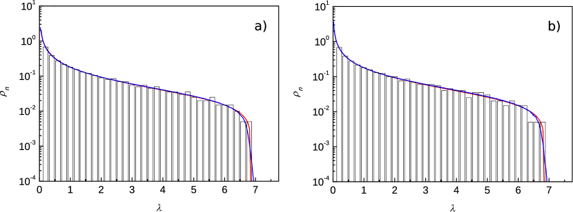
Figure 1: The eigenvalue density (in the semi-log scale) of the random matrix $M_{n}^{L}$ (1.12) for the Gaussian weights and biases. The network depth $L=2$ and the layer width $n=10^{3}$. The histograms correspond to the density of a sample of $M_{10^{3}}^{2}$, the solid blue curves to the arithmetic means $\rho_{n}$ of the sample densities of $N=10^{3}$ samples of $M_{10^{3}}^{2}$ and the solid red line to the numerical solution of equations (2.30) – (2.32). a) The linear activation function (conventional random matrix theory); b) the HardTanh activation function (2.54).

Figure 1. The eigenvalue densities of the random matrix $M_{n}^{L}$ (1.12) for $L=2$ and $n=10^{3}$. The histograms are obtained from the sample of $M_{10^{3}}^{2}$, the solid blue curves is the plot of the arithmetic means $\rho_{n}$ over $N=10^{3}$ samples of $M_{10^{3}}^{2}$ and the solid red curves are the result of the numerical solutions of equation (2.30) – (2.32), where the operation $diamond$ is given by (2.15) – (2.17). a) Linear activation function, b) The HardTanh activation function, i.e.,

$$a)\;\varphi(x)=x,\;\;\;b)\;\varphi=\left\{\begin{array}[]{cc}-1,&x\leq-1,\\ x,&|x|\leq 1,\\ +1,&x\geq 1.\end{array}\right.$$ (2.54)

The figure demonstrates the quite good fitting of the three descriptions of the eigenvalue density, thereby manifesting the fast convergence of the numerically obtained results to to a non-random limit given by Theorems 2.1 – 2.5.

Figure 2. a) displays the density $\nu_{K}^{\prime}$ of the measure $\nu_{K}$ of (2.31) for the indicated activation functions $\varphi$. It is well seen that all (except $\varphi(x)=x$) activation functions lead to quite similar $\nu_{K}^{\prime}$ having two narrow peaks centered at $0$ and $1$ and being rather close to zero otherwise. This is natural (in fact, exact) for the HardTanh (2.54), seems likely for the smooth sigmoid $\varphi(x)=\tanh x$, less likely for $\varphi(x)=\sinh x$ and rather surprising for $\varphi(x)=\sin x$. Nevertheless, according to Fig. 2b), the mean eigenvalue densities $\rho_{n}$ obtained from $N=10^{4}$ samples of $M_{10^{3}}^{2}$ for all $\varphi$ including $\varphi(x)=x$ are very close within the (semi-log) scale of the figure.

The weak dependence of $\rho_{n}$ on $\varphi$ can be viewed as an analog of the macroscopic universality (the universality of the global regime) in random matrix theory [22, 23], where the limiting eigenvalue distribution of the Wigner matrices and the sample covariance matrices are completely determined just by the second moment of the matrix entries. An analog of this type universality is also proved in this paper (we believe that condition on the fourth moment in (1.6) can be removed).

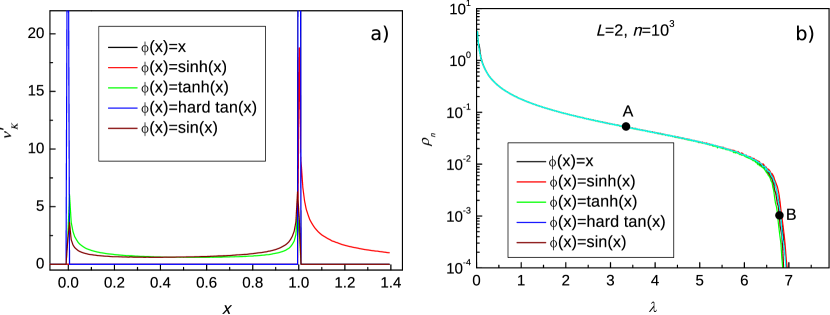
Figure 2: a) The density $\nu_{K}^{\prime}$ of the measure $\nu_{K}$ of (2.31) for the indicated activation functions and the Gaussian weights and biases. b) The arithmetic means $\rho_{n}$ (in the semi-log scale) of the sample eigenvalue densities of $M_{10^{3}}^{2}$ over $N=10^{4}$ samples for all indicated $\varphi$.

Note, however, that the "universality" shown in Fig. 2 is not exact. Indeed, by using a more refined scale for the curves of Fig. 2 b), we found that curves differ by $2.1\%$ in a neighborhood of $\ A$ and by $1.5\%$ in a neighborhood of $B$. In addition, it follows from Theorem 2.1 that if $\nu_{K^{\prime}}\neq\nu_{K^{\prime\prime}}$, then $\nu_{(M^{L})^{\prime}}$ $\neq\nu_{(M^{L})^{\prime\prime}}$. However, this fact could be of interest for applications, since it implies that up to a certain precision one can confine oneself to a simple case of linear, i.e., the standard random matrix, results and calculations. It is instructive in this context to consider the following family of activation functions:

$$\varphi_{\varepsilon}(x)=\varepsilon^{-1}\psi(\varepsilon x),$$ (2.55)

where $\psi:\mathbb{R}\rightarrow\mathbb{R},\;\psi(x)=x+o(x),\;x\rightarrow 0$ (sigmoid or not) is bounded and continuous. We have then for any $x$: $\varphi_{\varepsilon}(x)=x(1+o(1)),\;\varphi_{\varepsilon}^{\prime}(x)=1+o(1),\;\varepsilon\rightarrow 0$. We conclude that the linear case $\varphi(x)=x$ can be viewed as an asymptotic regime for the family (2.55). It is remarkable, however, that according to Fig. 2 the regime seems to be applicable up to $\varepsilon\simeq 1$. An analogous property was found in [39] although in a different context.

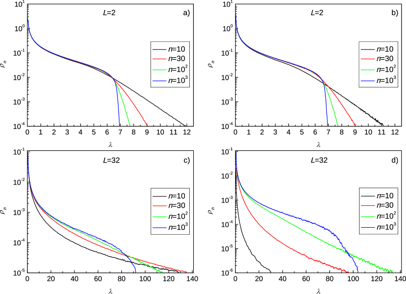
Figure 3: The arithmetic means $\rho_{n}$ (in the semi-log scale) of the sample eigenvalue densities of $M_{n}^{L}$ for various $L$, $n$ and $\varphi$ obtained by averaging over $N=10^{7}$ samples for $n=10,\;30$, $N=10^{6}$ samples for $n=10^{2}$ and $N=10^{4}$ samples for $n=10^{3}$. Figures a) and c) correspond to linear activation function $\varphi$, figures b) and d) correspond to the Hard-Tanh activation function (see (2.54)).

Figure 3 shows (in the semi-log scale) the arithmetic means $\rho_{n}$ of the sample eigenvalue densities of $M_{n}^{L}$ (1.12) with Gaussian weights and biases for various $L$, $n$ and $\varphi$ obtained from $N$ samples chosen according to (2.50). The "rows" of the figure, i.e., Fig. 3a) – Fig. 3b) and Fig. 3c) – 3d), describe the variation of $\rho_{n}$ in $n$ and $\varphi$ for a fixed $L=2,32$, while the "columns" of the figure, i.e., Fig. 3a) – Fig. 3c) and Fig. 3b) – 3d), describe the variation of $\rho_{n}$ in $n\,$ and $L$ for a fixed $\varphi$, the linear or the HardTanh (2.54). We observe the mentioned above similarity ("universality") of curves corresponding to different $\varphi^{\prime}$, the stronger dependence of curves on $n$ and stronger fluctuations in $L$, especially near the upper edge $a_{L}$ of the support and for the (non-smooth) HardTanh $\varphi$. It is also well seen the growth of $a_{L}$ in $L$. It is instructive to compare these properties of $\rho_{n}$ and those of the simplest case of $M_{n}^{L}$ with $R_{n}=D_{n}=\mathbf{1}_{n}$ (see (1.12)), where we have for the infinite width limit of the Stieltjes transform $f_{L}$ and the eigenvalue density $\rho_{L}$ (see [22], Problem 7.6.4): $z^{L}(-f_{L}(z))^{L+1}+zf_{L}(z)+1=0$ and

$$\rho_{L}(\lambda) = const.\ \lambda^{-\alpha_{L}}(1+o(1)),\;\lambda\downarrow 0,\;\;\alpha_{L}=L/(L+1),$$

$$\rho_{L}(\lambda) = const.\ (a_{L}-\lambda)^{1/2}(1+o(1)),\;\lambda\uparrow a_{L},\;$$

$$a_{L} = L(1+L^{-1})^{L+1}=Le(1+o(1)),\;L\rightarrow\infty.$$ (2.56)

It follows from the above that the support of $\rho_{L}$ grows in $L$ as well as its singularity at zero. Moreover, it is easy to see that $\lim_{L\rightarrow\infty}f_{L}(z)=-z^{-1}$, hence, the limiting $\rho_{\infty}$ is the Dirac delta at zero. The last property is valid in general case of $M_{n}^{L}$ of (1.12) and can be obtained either by the free probability argument [1, 27] or by using Theorems 2.5 and 2.1. Note that the subsequent limits $n\to\infty$ and then $L\to\infty$ can be viewed as an implementation of the heuristic inequality $1\ll L\ll n$. For another implementation where $L\to\infty,\;n\to\infty,\;L=o(n)$ (the double scaling limit in the terminology of statistical mechanics) see [1].

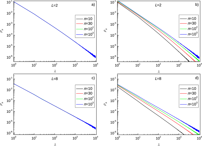
Figure 4: The arithmetic means $\rho_{n}$ (in the double-log scale) of the sample eigenvalue densities of $M_{n}^{L}$ with the Cauchy distributed weights and biases (see (2.49)) for various $L$, $n$ and $\varphi$ obtained by averaging over $N=10^{7}$ samples for $n=10,\;30$, $N=10^{6}$ samples for $n=10^{2}$ and $N=10^{4}$ samples for $n=10^{3}$. Figures a) and c) correspond to linear activation function $\varphi$, figures d) and d) correspond to the Hard-Tanh activation function (see (2.54)).

Figure 4 shows (in the double log-scale) the arithmetic means $\rho_{n}$ of the sample eigenvalue densities of $M_{n}^{L}$ (1.12) with the Cauchy distributed (2.49) weights and biases for various $L$, $n$ and $\varphi$ obtained from $N$ samples chosen according to (2.50). The figure is organized similarly to Figure 3, i.e., its "rows", Fig. 4a) – Fig. 4b) and Fig. 4c) – 4d), describe the variation of $\rho_{n}$ in $n$ and $\varphi$ for a fixed $L=2,8$, while the "columns", Fig. 4a) – Fig. 4c) and Fig. 4b) – Fig. 4d), describe the variation of $\rho_{n}$ $n\,$ and $L$ for a fixed $\varphi$, the linear or the HardTanh, see (2.54).

As seen from the pictures, for linear $\varphi$ the density $\rho_{n}$ is well described by the power law dependence $\rho_{n}(\lambda)\sim\lambda^{-\alpha}$ in a sufficient wide range of its argument with $\alpha\approx 1.25$ for network depth $L=2$ and $\alpha\approx 1.05$ for $L=8$. More detailed analysis shows that for "small" $\lambda$ ($0\leq\lambda\lesssim 10$) the curve $\rho_{n}$ deviates from the straight line and can be described for of sufficiently small $\lambda$’s by the power law with the exponent $\alpha\approx 0.7$ for network depth $L=2$ and $\alpha\approx 0.9$ for $L=8$.

We observe also a certain similarity of Figure 4 and Figure 3, e.g., the stronger dependence of curves on $n$ and stronger fluctuations in $L$, especially for the case of non-smooth HardTanh $\varphi$ (not covered by Theorem 2.5).

Note that our analytic results do not apply to this case, since the Cauchy distribution does not satisfy conditions (1.5) - (1.6). We present here these numerical results, firstly in order to demonstrate an example of a rather different behavior of the eigenvalue distribution density and, secondly, because of existing indications in the literature on the possibility of using random matrices with the "heavy-tailed" distributed entries in the deep neural networks studies, see the review [10] and references therein.

For more pictures of the eigenvalue distribution of $M_{n}^{L}$ and the related characteristics of the scheme (1.1) – (1.4) see [1, 13, 20] and references therein.

3 Proof of Theorem 2.1.

We begin with the list of facts of linear algebra and probability theory that are used in the proof of Theorem 2.1.

Proposition 3.1

Let $A$ and $B$ be $n\times n$ real symmetric matrices and $L_{Y}$ be the rank one real symmetric matrix corresponding to the vector $Y=\{Y_{\alpha}\}_{\alpha=1}^{n}\in\mathbb{C}^{n}$, i.e.,

$$L_{Y}=\{L_{\alpha\beta}\}_{\alpha,\beta=1}^{n},\;L_{\alpha\beta}=Y_{\alpha}Y_{\beta}.$$ (3.1)

We have:

(i)

$$\mathrm{Tr}AL_{Y}=(AY,Y)$$ (3.2)

(ii) if

$$G_{A}(z)=(A-z)^{-1},\;G_{B}(z)=(B-z)^{-1},\;\Im z\neq 0,$$ (3.3)

are the resolvents of $A$ and $B$, then the resolvent identity

$$G_{A}(z)=G_{B}(z)-G_{A}(z)(A-B)G_{B}(z),\;\Im z\neq 0$$ (3.4)

is valid;

(iii) if $K$ is a real number and

$$A=B+KL_{Y},$$ (3.5)

where $L_{Y}$ is given by (3.1), then the rank one perturbation formula

$$G_{A}(z)=G_{B}(z)-\frac{K}{1+K(G_{B}(z)Y,Y)}G_{B}(z)L_{Y}G_{B}(z),\;\Im z\neq 0$$ (3.6)

is valid, if $C$ is one more $n\times n$ matrix (not necessarily hermitian), then

$$n^{-1}\mathrm{Tr}G_{A}(z)C-n^{-1}\mathrm{Tr}G_{B}(z)C=-\frac{1}{n}\cdot\frac{K(G_{B}(z)CG_{B}(z)Y,Y)}{1+K(G_{B}(z)Y,Y)}$$ (3.7)

and if $B$ is positive definite and $K\geq 0$, then

$$|n^{-1}\mathrm{Tr}G_{A}(-\xi)C-n^{-1}\mathrm{Tr}G_{B}(-\xi)C|\leq||C||/n\xi,\;\xi>0;$$ (3.8)

(iv) if $X=\{X_{\alpha}\}_{\alpha=1}^{n}\in\mathbb{R}^{n}$ is a random vector with jointly independent and identically distributed real components and (cf. (1.6) and (2.3))

$$\mathbf{E}\{X_{\alpha}\}=0,\;\mathbf{E}\{X_{\alpha}^{2}\}=1,\;\mathbf{E}\{X_{\alpha}^{4}\}=m_{4}<\infty,$$ (3.9)

where $\mathbf{E}\{\dots\}$ denotes the corresponding expectation, and

$$Y=n^{-1/2}SX,$$ (3.10)

with a $X$-independent $n\times n$ real symmetric matrix $S$, then

$$\mathbf{E}\{L_{Y}\}=n^{-1}R,\;R=S^{2}$$ (3.11)

and if

$$a=(CY,Y),$$ (3.12)

is a quadratic form with a $X$-independent and not necessarily hermitian $C$, then

$$\mathbf{E}\{a\}=n^{-1}\mathrm{Tr}\,CR=n^{-1}\mathrm{Tr}\,C_{S},\;C_{S}=SCS$$ (3.13)

and

$$\mathbf{Var}\{a\}:=\mathbf{E}\{|a|^{2}\}-|\mathbf{E}\{a\}|^{2}\leq\mu\;\mathrm{Tr}\,C_{S}C_{S}^{\ast}/n^{2},\;\mu=m_{4}+1,$$ (3.14)

where $C^{\ast}$ is the hermitian conjugate of $C$ (recall that $m_{4}\in[1,\infty)$ in view of (3.9)).

Proof. Assertions (i) and (ii) are elementary.

(iii). To obtain (3.6) we use (3.4) with $A$ and $B$ of (3.5) to write the formula

$$G_{A}(z)=G_{B}(z)-KG_{A}(z)LG_{B}(z).$$ (3.15)

Multiplying it by $L$ of (3.1) from the right and using $LG_{B}(z)L=(G_{B}(z)Y,Y)L$, we get

$$G_{A}(z)L=(1+K(G_{B}(z)Y,Y))^{-1}G_{B}(z)L.$$ (3.16)

Plugging this into the r.h.s. of (3.15), we obtain (3.6) and then (3.7).

Note that the r.h.s. of (3.6) and (3.7) are well defined for $\Im z\neq 0$. Indeed, it follows from (3.4) with $A-z$ as $A$ and  $A-z^{\ast}$as $B$ that

$$\Im G(z)=(2i)^{-1}(G-G^{\ast})=\Im z\ G^{\ast}(z)G(z),$$

thus

$$|1+K(G_{B}(z)Y,Y)|\geq|K\Im(G_{B}(z)Y,Y)|=|K|\ |\Im z|\ ||G_{B}(z)Y||^{2}>0,\ \Im z\neq 0.$$

To get (3.8) we take into account that $K\geq 0$ and $(G_{B}(-\xi)Y,Y)\geq 0$, since $B$, hence, $G_{B}(-\xi)$ is positive definite. This yields the following bound for the r.h.s. of (3.7)

$$||C||\,||G_{B}(-\xi)Y)||^{2}/(G_{B}(-\xi)Y,Y)=||C||(G_{B}^{2}(-\xi)Y,Y)/(G_{B}(-\xi)Y,Y)$$

implying

$$(G_{B}(-\xi)Y,Y)=(G_{B}^{-1}(-\xi)G_{B}^{2}(-\xi)Y,Y)=((B+\xi)G_{B}^{2}(-\xi)Y,Y)$$

$$\hskip 42.67912pt=(G_{B}(-\xi)BG_{B}(-\xi)Y,Y)+\xi(G_{B}^{2}(-\xi)Y,Y)\geq\xi(G_{B}^{2}(-\xi)Y,Y).$$

(iv) We use the formulas (see (3.9))

$$\mathbf{E}\{X_{\alpha_{1}}X_{\alpha_{2}}\}=\delta_{\alpha_{1}\alpha_{2}},$$

$$\mathbf{E}\{X_{\alpha_{1}}X_{\alpha_{2}}X_{\alpha_{3}}X_{\alpha_{4}}\} =\delta_{\alpha_{1}\alpha_{2}}\delta_{\alpha_{3}\alpha_{4}}+\delta_{\alpha_{1}\alpha_{3}}\delta_{\alpha_{2}\alpha_{4}}$$

$$\hskip 8.5359pt+\delta_{\alpha_{1}\alpha_{4}}\delta_{\alpha_{2}\alpha_{3}}+(m_{4}-3)\delta_{\alpha_{1}\alpha_{2}}\delta_{\alpha_{1}\alpha_{3}}\delta_{\alpha_{1}\alpha_{4}}.$$

The first line above, (3.1) and (3.10) yields (3.11) and (3.13), while the second line implies

$$\mathbf{E}\{|a|^{2}\} = n^{-2}|\mathrm{Tr\,}C_{S}|^{2}+n^{-2}\sum_{\alpha\neq\beta=1}^{n}|(C_{S})_{\alpha\beta}|^{2}$$

$$+n^{-2}\sum_{\alpha\neq\beta=1}^{n}(C_{S})_{\alpha\beta}(C_{S})_{\beta\alpha}^{\ast}+(m_{4}-1)n^{-2}\sum_{\alpha=1}^{n}|(C_{S})_{\alpha\alpha}|^{2}.$$

The sums of the r.h.s. are bounded by

$$n^{-2}\sum_{\alpha\neq\beta=1}^{n}|(C_{S})_{\alpha\beta}|^{2}=n^{-2}\mathrm{Tr\,}C_{S}C_{S}^{\ast}$$

and $m_{4}\geq 1$ in view of (3.9). This leads (3.14).   

We will prove now Theorem 2.1.

Proof. We begin with using Lemma 3.4 (i) below implying that the fluctuations (3.77) of $\nu_{\mathcal{M}_{n}}$ vanish sufficiently fast as $n\rightarrow\infty$. This and the Borel-Cantelli lemma imply that

$$\lim_{n\to\infty}|\nu_{\mathcal{M}_{n}}(\Delta)-\mathbf{E}\{\nu_{\mathcal{M}_{n}}(\Delta)\}|=0$$

with probability 1, hence reduce the proof of the theorem to the proof of the weak convergence of the expectation

$$\overline{\nu}_{\mathcal{M}_{n}}:=\mathbf{E}\{\nu_{\mathcal{M}_{n}}\}$$ (3.17)

of $\nu_{\mathcal{M}_{n}}$ to the limit $\nu_{\mathcal{M}}$ whose Stieltjes transform is given by (2.15) – (2.19). Since $\mathcal{M}_{n}$ is positive definite, hence, its spectrum belongs to the closed positive semiaxis $\mathbb{R}_{+}$ for all $n$, it suffices to prove the tightness of the sequence of measures $\{\overline{\nu}_{\mathcal{M}_{n}}\}_{n}$ and the pointwise convergence on a set of positive Lebesgue measure in $\mathbb{C}\setminus\mathbb{R}_{+}$ of their Stieltjes transforms (cf. (1.20))

$$f_{\mathcal{M}_{n}}(z):=\int_{0}^{\infty}\frac{\overline{\nu}_{\mathcal{M}_{n}}(d\lambda)}{\lambda-z},\;\mathbb{C}\setminus\mathbb{R}_{+}$$ (3.18)

to the limit satisfying (2.15) – (2.19), see, e.g. [22], Proposition 2.1.2.

The tightness is guaranteed by the uniform in $n$ bound for

$$\mu_{n}^{(1)}:=\int_{0}^{\infty}\lambda\overline{\nu}_{\mathcal{M}_{n}}(d\lambda),$$ (3.19)

since for any $T>0$ we have for the tail of $\overline{\nu}_{\mathcal{M}_{n}}$

$$\int_{T}^{\infty}\overline{\nu}_{\mathcal{M}_{n}}(d\lambda)\leq T^{-1}\int_{T}^{\infty}\lambda\overline{\nu}_{\mathcal{M}_{n}}(d\lambda)\leq\mu_{n}^{(1)}/T.$$

According to the definition of the NCM (see, e.g. (1.16)), spectral theorem and (2.4), we have

$$\mu_{n}^{(1)}=\mathbf{E}\{n^{-1}\mathrm{Tr}\,\mathcal{M}_{n}\}=\mathbf{E}\{n^{-2}\mathrm{Tr}\,X_{n}R_{n}X_{n}^{T}K_{n}\}$$

and then (2.47), (2.5) – (2.7) and (2.10) – (2.11) yield

$$\mu_{n}^{(1)}\leq n^{-2}\Phi_{1}^{2}\mathbf{E}\{\mathrm{Tr}\,X_{n}R_{n}X_{n}^{T}\}=\Phi_{1}^{2}n^{-1}\mathrm{Tr}\,R_{n}\leq r_{2}^{1/2}\Phi_{1}^{2},$$ (3.20)

where we used the inequality $n^{-1}\mathrm{Tr}\,R_{n}\leq(n^{-1}\mathrm{Tr}\,R_{n}^{2})^{1/2}$ to obtain the r.h.s. bound. This implies the tightness of $\{\overline{\nu}_{\mathcal{M}_{n}}\}_{n}$ and reduces the proof of the theorem to the proof of pointwise in $\mathbb{C}\setminus\mathbb{R}_{+}$ convergence of (3.18) to the limit determined by (2.15) – (2.17).

The above argument, reducing the analysis of the large size behavior of the eigenvalue distribution of random matrices to that of the expectation of the Stieltjes transform of the distribution, is widely used in random matrix theory (see [22], Chapters 3, 7, 18 and 19), in particular, while dealing with the sample covariance matrices. However, the matrix $\mathcal{M}_{n}$ of (2.4) differs essentially from the sample covariance matrices, since the "central" matrix $K_{n}$ of (2.10) is random and dependent on $X_{n}$ (the data matrix according to statistics), while in the sample covariance matrix the analog of $K_{n}$ is either deterministic or random but independent of $X_{n}$. Nevertheless, we show that in our case of the $X_{n}$-dependent $K_{n}$ of (2.10) it suffices to follow essentially the proof for $X_{n}$-independent analogs of $K_{n}$, which dates back to [31, 32] and has been largely extended and used afterwards, see, e.g. [22, 33, 34, 35].

We outline first the scheme of the proof of the theorem. Write (2.4) as

$$\mathcal{M}_{n}=\sum_{j=1}^{n}K_{jn}L_{jn},$$ (3.21)

where $K_{jn}$ are given by (2.10) and

$$L_{jn}=L_{Y_{j}}$$ (3.22)

is the rank-one matrix (3.1) corresponding to the random vector (cf. (3.10))

$$Y_{j}=\{n^{-1/2}(S_{n}X_{n}^{T})_{j\alpha}\}_{\alpha=1}^{n}=n^{-1/2}S_{n}X_{j},\;X_{j}=\{X_{j\alpha}\}_{\alpha=1}^{n},$$ (3.23)

i.e., $X_{j}$ is the $j$th row of the random matrix (2.7), thus the collection $\{X_{j}\}_{j=1}^{n}$ consists of i.i.d. random vectors satisfying (3.9).

It follows from the definition of the Normalized Counting Measure (see (1.16)) and the spectral theorem for the resolvent

$$G_{\mathcal{M}_{n}}(z)=(\mathcal{M}_{n}-z)^{-1}$$ (3.24)

of $\mathcal{M}_{n}$ that

$$f_{\mathcal{M}_{n}}(z)=\mathbf{E}\{n^{-1}\mathrm{Tr}\,G_{\mathcal{M}_{n}}(z)\}.$$ (3.25)

Hence, we have to deal with $G_{\mathcal{M}_{n}}(z)$.

By using the resolvent identity (3.4) for $A=\mathcal{M}_{n}$ and $B=0$, we obtain for (3.24) in view of (3.21)

$$G(z)=-z^{-1}+z^{-1}\sum_{j=1}^{n}K_{j}G(z)L_{j},$$ (3.26)

and we omit here and below the subindex $\mathcal{M}_{n}$ in the resolvent (3.24) as well as the subindex $n$ in many instances below where this does no lead to confusion.

Next, we choose in (3.6)

$$A=\mathcal{M}_{n},\;B=\mathcal{M}_{n}^{(j)}:=\mathcal{M}_{n}-K_{j}L_{j}$$ (3.27)

and use (3.16) to obtain

$$G(z)L_{j}=G_{j}(z)L_{j}(1+K_{j}a_{j}(z))^{-1},\;a_{j}(z):=(G_{j}(z)Y_{j},Y_{j}),$$ (3.28)

where

$$G_{j}(z):=(\mathcal{M}_{n}^{(j)}-z)^{-1}$$ (3.29)

and $Y_{j}$ is defined in (3.23). Plugging (3.28) into (3.26), we obtain our basic starting formula

$$G(z)=-z^{-1}+z^{-1}\sum_{j=1}^{n}\frac{K_{j}}{(1+K_{j}a_{j}(z))}G_{j}(z)L_{j}$$ (3.30)

which we are going to convert into the "prelimit" version of the system (2.15) – (2.17) plus error terms vanishing as $n\rightarrow\infty$.

It follows from (3.25) that we are allowed to make any modification of (3.30) provided that the corresponding error term $\mathcal{E}_{n}$ satisfies

$$\mathbf{E}\{n^{-1}\mathrm{Tr}\,\mathcal{E}_{n}\}=o(1),\;n\rightarrow\infty.$$ (3.31)

Denote $\mathbf{E}_{j}\{...\}$ the operation of expectation conditioned on $\{X_{k}\}_{k\neq j}$ and use:

(i) (3.9) – (3.14) and (3.23) to replace the random quadratic form $(CY_{j},Y_{j})$ with a $Y_{j}$-independent matrix $C$ by

$$\mathbf{E}_{j}\{(CY_{j},Y_{j})\}=n^{-1}\mathbf{E}_{j}\{(C_{S}X_{j},X_{j})\}=n^{-1}\mathrm{Tr}\,CR;$$ (3.32)

(ii) (3.7) – (3.8) to replace $n^{-1}\mathrm{Tr}G_{j}(z)C$ with a $Y_{j}$-independent $C$ by $n^{-1}\mathrm{Tr}\,G(z)C$;

(iii) Lemma 3.4 to replace the random variable $n^{-1}\mathrm{Tr}\,G(z)C$ with a $Y_{j}$-independent matrix $C$ by the expectation $\mathbf{E}\{n^{-1}\mathrm{Tr}\,G(z)C\}$.

We will apply then: (i) with $C=G_{j}$ to replace $a_{j}(z)$ of (3.28) by

$$h_{jn}(z)=n^{-1}\mathrm{Tr}\,RG_{j}(z),$$ (3.33)

(ii) with $C=R$ to replace $h_{jn}(z)$ by $h_{n}(z)$ and then (iii) with $C=R$ to replace $h_{n}(z)$ by $\overline{h_{n}}(z)$, where

$$h_{n}(z)=n^{-1}\mathrm{Tr}\,RG(z)=n^{-1}\mathrm{Tr}\,SG(z)S,\;\;\overline{h_{n}}(z)=\mathbf{E}\{h_{n}(z)\}.$$ (3.34)

As a result, we can replace $(1+K_{j}a_{j}(z))$ by $(1+K_{j}\overline{h_{n}}(z))$ in the r.h.s. of (3.30), see Lemma 3.3 for details.

Likewise, we can replace $L_{j}$ in (3.30) by its expectation $n^{-1}R$ by using (i) and then replace $G_{j}(z)$ by $G(z)$ by using (ii) to convert (3.30) into

$$G(z)=-z^{-1}+z^{-1}\overline{k}_{n}(z)G(z)R+T_{1}(z),$$ (3.35)

where

$$k_{n}(z)=\frac{1}{n}\sum_{j=1}^{n}\frac{K_{j}}{1+K_{j}\overline{h}_{n}(z)},\;\overline{k}_{n}(z)=\mathbf{E}\{k_{n}(z)\}$$ (3.36)

and

$$T_{1}(z)=z^{-1}\sum_{j=1}^{n}\frac{K_{j}}{1+K_{j}a_{j}(z)}G_{j}(z)L_{j}-z^{-1}\overline{k}_{n}(z)G(z)R.$$ (3.37)

is the error term.

Applying to (3.35) the operation $\mathbf{E}\{n^{-1}\mathrm{Tr\;}\dots\}$ and taking into account (3.25) and (3.34), we get

$$f_{\mathcal{M}_{n}}(z)=-z^{-1}+z^{-1}\overline{k}_{n}(z)\overline{h}_{n}(z)+t_{1n},$$ (3.38)

where

$$t_{1n}(z)=\mathbf{E}\{n^{-1}\mathrm{Tr}\,T_{1}(z)\},$$ (3.39)

i.e., a "prelimit" version of (2.15) with the error term $t_{1n}$, cf. (3.31).

Next, we have from (3.35)

$$G(z)=\mathcal{G}(z)+zT_{1}\mathcal{G}(z),\;\mathcal{G}(z)=(\overline{k}_{n}(z)R-z)^{-1}.$$ (3.40)

Multiplying the formula by $R$, applying to the result the operation $\mathbf{E}\{n^{-1}\mathrm{Tr\;}...\}$ and using the fact that $R$ of (2.5), hence, $\mathcal{G}$ are independent of $X_{n}$ of (2.7), we obtain in view of (3.34)

$$\overline{h}_{n}(z)=\int_{0}^{\infty}\frac{\lambda\nu_{R_{n}}(d\lambda)}{\lambda\overline{k}_{n}(z)-z}+t_{2n},$$ (3.41)

where $\nu_{R_{n}}$ is the Normalized Counting Measure of $R_{n}$ defined in (2.6). This is a "prelimit" version of (2.16) with the error term (cf. (3.31) and (3.39))

$$t_{2n}(z)=-z\mathbf{E}\{n^{-1}\mathrm{Tr}\,T_{1}\mathcal{G}(z)R\}.$$ (3.42)

At last, observing that according to the conditions of the theorem (see (2.7), (1.4) and (2.10)) $\{K_{j}\}_{j=1}^{n}$ are independent identically distributed (and, possibly, $n$-dependent) random variables, we obtain from (3.36) the "prelimit version"

$$\overline{k}_{n}(z)=\int_{0}^{\infty}\frac{\lambda\overline{\nu}_{K_{n}}(d\lambda)}{\lambda\overline{h}_{n}(z)+1}$$ (3.43)

of (2.17) in which $\overline{\nu}_{K_{n}}$ is the probability law of (see (2.10))

$$K_{jn}=(\varphi^{\prime}(\eta_{jn}+b_{j}))^{2},\;\eta_{jn}=n^{-1/2}\sum_{\alpha=1}^{n}X_{j\alpha}x_{\alpha n}.$$ (3.44)

Having obtained semi-heuristically relations (3.38), (3.41) and (3.43), we pass now to their rigorous derivation, i.e., to the proof that the remainders $t_{1n}$ of (3.39) and $t_{2n}$ of (3.42) vanish in the limit $n\rightarrow\infty$ and that $f_{\mathcal{M}_{n}}$, $\overline{h}_{n}$ and $\overline{k}_{n}$ converge to a solution of (2.15) – (2.17).

We will deal first with the $n\to\infty$ limit in (3.38), (3.43) and (3.41) assuming that $t_{1n}$ and $t_{2n}$ vanish as $n\rightarrow\infty$. In fact, the limit is a version of that widely used in random matrix theory, see, e.g. [22]. Thus, we just outline the procedure.

According to (3.18) $f_{\mathcal{M}_{n}}$ is analytic in $\mathbb{C}\setminus\mathbb{R}_{+}$ for every $n$. Thus, by Vitali’s theorem on the convergence of analytic functions, it suffices to study the limiting properties of the sequence $\{f_{\mathcal{M}_{n}}\}_{n}$ for $z$ varying in a closed interval of the open negative semiaxis

$$I_{-}=\{z\in\mathbb{C}:z=-\xi,\;0<\xi_{-}\leq\xi\leq\xi_{+}<\infty\},$$ (3.45)

where $\xi_{\pm}$ do not depend on $n$.

Furthermore, since $\mathcal{M}_{n}$ of (2.4) and $\mathcal{M}_{n}^{(j)}$ of (3.27) are positive definite, their resolvents $G(z)$ and $G_{j}(z)$ for $z=-\xi\in I_{-}$ are also positive definite, thus

$$||G(-\xi)||\leq 1/\xi,\;||G_{j}(-\xi)||\leq 1/\xi,\;\;\xi>0,$$ (3.46)

and we have for $a_{j}$ of (3.28)

$$a_{j}(-\xi)\geq 0,\;\xi>0.$$ (3.47)

Besides, we have from (2.10) and (2.11)

$$0\leq K_{j}\leq\Phi_{1}^{2}.$$ (3.48)

Thus, $1+K_{j}a_{j}(-\xi)\geq 1$ and (3.28) is well defined for $\xi>0$.

It follows from (3.34), spectral theorem for $\mathcal{M}_{n}$ and (2.5) that if $\{\lambda_{\alpha}\}_{\alpha}$ and $\{\psi_{\alpha}\}_{\alpha}$ are the eigenvalues and the eigenvectors of $\mathcal{M}_{n}$, then

$$h_{n}(z)=\int_{0}^{\infty}\frac{\mu_{n}(d\lambda)}{\lambda-z},\;z\in\mathbb{C}\setminus\mathbb{R}_{+},$$

$$\hskip 14.22636pt\mu_{n}=n^{-1}\sum_{\alpha}\delta_{\lambda_{\alpha}}(R\psi_{\alpha},\psi_{\alpha}),\;$$

$$0<\mu_{n}(\mathbb{R}_{+})=n^{-1}\sum_{\alpha}(R\psi_{\alpha},\psi_{\alpha})=n^{-1}\mathrm{Tr}\,R\leq r_{2}^{1/2},$$ (3.49)

where we took into account that $R$ is positive defined and used Schwarz inequality for traces. This implies that $h_{n}$ is analytic in $\mathbb{C}\setminus\mathbb{R}_{+}$ and

$$\Im h_{n}(z)\Im z=\int_{0}^{\infty}\frac{\mu_{n}(d\lambda)}{|\lambda-z|^{2}}>0,\;\Im z\neq 0.$$ (3.50)

In particular, the function $\overline{k}_{n}$ of (3.36) is also analytic in $\mathbb{C}\setminus\mathbb{R}_{+}$.

It follows also from the above and (3.18) that

$$0<f_{\mathcal{M}_{n}}(-\xi)\leq 1/\xi,\;\;0<\overline{h}_{n}(-\xi)\leq r_{2}^{1/2}/\xi,\;\;0<\overline{k}_{n}(-\xi)\leq 1,\;\;\xi>0.$$ (3.51)

Moreover, since the sequences $\{f_{\mathcal{M}_{n}}\}_{n},\;\{\overline{h}_{n}\}_{n}$ and $\{\overline{k}_{n}\}_{n}$ are real analytic on $I_{-}$ of (3.45), there exists a subsequence $n_{j}\rightarrow\infty$ such that $\{f_{\mathcal{M}_{n_{j}}}\},\{\overline{h}_{n_{j}}\}$ and $\{\overline{k}_{n_{j}}\}$ converge uniformly on (3.45) to certain limits $f_{\mathcal{M}},h$ and $k$ analytic in $\mathbb{C}\setminus\mathbb{R}_{+}$. This allows us to carry out the limit along $n_{j}\rightarrow\infty$ in the second term in the r.h.s. of (3.38) and to obtain (2.15) provided that $t_{1n_{j}}$ vanishes as $n_{j}\rightarrow\infty$.

Next, write the first term in the r.h.s. of (3.41) for $z=-\xi\in I_{-}$ as

$$\int_{0}^{\infty}\frac{\lambda\nu_{R_{n_{j}}}(d\lambda)}{\lambda k(-\xi)+\xi}+(\overline{k}_{n_{j}}(-\xi)-k(-\xi))\int_{0}^{\infty}\frac{\lambda^{2}\nu_{R_{n_{j}}}(d\lambda)}{(\lambda k(-\xi)+\xi)(\lambda\overline{k}_{n_{j}}(-\xi)+\xi)}.$$

It follows then from (2.5), (2.6) and (3.51) that the first term tends to the r.h.s. of (2.16) as $n_{j}\rightarrow\infty$. The integral in the second term is bounded by $r_{2}/\xi^{2}$ in view of (2.5) and (3.51), hence, the second term vanishes as $n_{j}\rightarrow\infty$. Thus, we obtain (2.16) provided that $t_{2n_{j}}$ vanishes as $n_{j}\rightarrow\infty$.

An analogous argument applies to (3.43). However, to obtain (2.17) and (2.18), we have to find the limiting probability law of the random variable $\eta_{jn}$ of (3.44). It follows from the standard facts on the Central Limit Theorem (see, e.g. [37], Section III.4), (3.9) and (2.12) that the law is Gaussian of zero mean and variance $q-\sigma_{b}^{2}$, see Lemma 3.5 for details. This proves (2.17).

Thus, we have proved the validity of (2.15) – (2.18) for $z\in I_{-}$ of (3.45) provided that $t_{1n}$ and $t_{2n}$ of (3.39) and (3.42) vanish uniformly in $z\in I_{-}$. It is shown in Lemma 3.7 that the system (2.16) – (2.17) is well defined and uniquely solvable everywhere in $\mathbb{C}\setminus\mathbb{R}_{+}$. This implies that the whole sequences $\{f_{\mathcal{M}_{n}}\},\{\overline{h}_{n}\}$ and $\{\overline{k}_{n}\}$ converge uniformly on any compact set of $\mathbb{C}\setminus\mathbb{R}_{+}$, that their limits $f_{\mathcal{M}},h$ and $k$ are not identically zero and can be found from relations (2.15) – (2.18) which are valid everywhere in $\mathbb{C}\setminus\mathbb{R}_{+}$. Indeed, if $h$ is identically zero, then it follows from (2.17) with $z=-\xi<0$ that $k(-\xi)=k_{1}>0\,$, where $k_{1}$ is the first moment of measure $\nu_{K}$ of (2.18). Then (2.16) implies that $\nu_{R}$ is concentrated at zero. This contradicts condition (a) of the theorem. Analogously, assuming that $k$ is identically zero, we conclude that $\nu_{K}$ of (2.18) is concentrated at zero and this is impossible if $\varphi$ is not identically constant.

Besides, it follows from (3.51) that $k(-\xi)$ and $\xi h(-\xi)$ are nonnegative and bounded. Thus, the limit $\xi\rightarrow\infty$ in (2.15) yields (2.14). Conditions (2.19) follow from the $n\to\infty$ versions of (3.49) – (3.51).

We pass now to the most technical part of the proof in which we establish that the error terms (3.39) and (3.42) vanish as $n\to\infty$ uniformly on $z\in I_{-}$ of (3.45).

Note first that it suffices to assume that the sequence $\{R_{n}\}$ of (2.4) – (2.6) is uniformly bounded, i.e.,

$$\sup_{n}||R_{n}||\leq\rho<\infty,$$ (3.52)

instead of (2.5). This is also a standard and technically convenient trick of random matrix theory where it is shown that once the limiting Normalized Counting Measure is found under condition (3.52), it can be also found under condition (2.5), see e.g. [22], Section 19, in particular, Theorem 19.1.8 for the case where $K_{n}$ is independent of $X_{n}$ of (2.7). In our case of (2.10) – (2.11) the proof of this fact is given in [2].

By using (3.37) and (3.39), we have from (3.2), (3.34) and (3.36)

$$t_{1n}(-\xi) =\frac{1}{zn}\sum_{j=1}^{n}\mathbf{E}\{a_{j}K_{j}(1+K_{j}a_{j})^{-1}-\overline{h}_{n}K_{j}(1+K_{j}\overline{h}_{n})^{-1}\}|_{z=-\xi}$$

$$=-\frac{1}{zn}\sum_{j=1}^{n}\mathbf{E}\{(a_{j}-\overline{h}_{n})K_{j}((1+K_{j}a_{j})(1+K_{j}\overline{h}_{n}))^{-1}\}|_{z=-\xi}.$$ (3.53)

It follows then from (3.47) – (3.51) that

$$(1+K_{j}a_{j}(-\xi))\geq 1,\;(1+K_{j}\overline{h}_{n}(-\xi))\geq 1.$$ (3.54)

These bounds, (3.51) and (3.53) imply

$$|t_{1n}(-\xi)|\leq\Phi_{1}^{2}d_{1}\xi^{-1},\;d_{1}=n^{-1}\sum_{j=1}^{n}d_{1j},\;d_{1j}=\mathbf{E}\{|a_{j}-\overline{h}_{n}|\}.$$ (3.55)

According to Lemma 3.3, $d_{1j}\leq C^{\prime}/n^{1/2}$ if $n$ is large enough and we obtain

$$|t_{1n}(-\xi)|\leq C_{1}/n^{1/2},\;C_{1}=\Phi_{1}^{4}C^{\prime}\xi^{-1}.$$ (3.56)

This and (3.38) justify (2.15).

Consider now $t_{2n}$ of (3.42). Using an argument similar to that leading to (3.53), we obtain

$$t_{2n}(-\xi) =n^{-1}\sum_{j=1}^{n}\mathbf{E}\{b_{j}K_{j}(1+K_{j}a_{j})^{-1}-\overline{c}_{n}K_{j}(1+K_{j}\overline{h}_{n})^{-1}\}|_{z=-\xi}$$

$$\hskip 56.9055pt=t_{2n}^{\prime}(-\xi)+t_{2n}^{\prime\prime}(-\xi),$$ (3.57)

where (cf. (3.28) and (3.34))

$$b_{j}=(R\mathcal{G}G_{j}Y_{j},Y_{j}),\;c_{n}=n^{-1}\mathrm{Tr}\,R^{2}\mathcal{G}G,\;\overline{c}_{n}=\mathbf{E}\{c_{n}\}$$ (3.58)

and (cf. 3.53)

$$t_{2n}^{\prime}(-\xi) =n^{-1}\sum_{j=1}^{n}\mathbf{E}\{(\overline{h}_{n}-a_{j})K_{j}^{2}\overline{c}_{n}((1+K_{j}a_{j})(1+K_{j}\overline{h}_{n}))^{-1}\}|_{z=-\xi},$$

$$t_{2n}^{\prime\prime}(-\xi) =n^{-1}\sum_{j=1}^{n}\mathbf{E}\{(b_{j}-\overline{c}_{n})(K_{j}+K_{j}^{2}\overline{h}_{n})((1+K_{j}a_{j})(1+K_{j}\overline{h}_{n}))^{-1}\}|_{z=-\xi}.$$ (3.59)

Since $R$ is positive definite, (3.51) implies for $\mathcal{G}$ of (3.40) (cf. (3.46))

$$||\mathcal{G}(-\xi)||\leq\xi^{-1}.$$ (3.60)

It follows then from (3.46), (3.52), (3.58) and (3.60) that

$$|\overline{c}_{n}|\leq\rho^{2}\xi^{-2}.$$ (3.61)

This, (3.48) and (3.54) yield

$$|t_{2n}^{\prime}(-\xi)|\leq\Phi_{1}^{4}\rho^{2}\xi^{-2}d_{1}$$ (3.62)

with $d_{1}$ of (3.55). Thus, Lemma 3.3 implies

$$|t_{2n}^{\prime}(-\xi)|\leq C_{21}/n^{1/2}$$ (3.63)

for a certain $n$-independent $C_{21}$.

Likewise, by using (3.48), (3.54) and (3.51), we obtain

$$|t_{2n}^{\prime\prime}(-\xi)|\leq(\Phi_{1}^{2}+\Phi_{1}^{4}r^{1/2}\xi^{-1})\ d_{2},\;\ d_{2}=n^{-1}\sum_{j=1}^{n}d_{2j},\;d_{2j}=\mathbf{E}\{|b_{j}-\overline{c}_{n}|\},$$ (3.64)

and then Lemma 3.3 implies $|t_{2n}^{\prime\prime}(-\xi)|\leq C_{22}/n^{1/2}$ for a certain $n$-independent $C_{22}$.

Combining this bound, (3.57) and (3.63), we get (cf. (3.56))

$$|t_{2n}(-\xi)|\leq C_{2}/n^{1/2}.$$ (3.65)

This and (3.41) justifies (2.16).   

Remark 3.2

It is noted at the beginning of Section 2 that despite the fact that the matrices $D^{l}$ of (1.11), hence $K_{n}^{l}$ of (1.23), are random and depend on $X^{l}$ of (1.6), the limiting eigenvalue distribution of $M_{n}^{L}$ of (1.12) corresponds to the case where $D^{l}$ of (1.11) and $K_{n}^{l}$ are random but independent of $X^{l}$, see (2.31) and (2.18). The emergence of this remarkable property of $M_{n}^{L}$ is well seen in the above proof, in particular, in formulas (3.35) – (3.44) and (3.56), (3.65). Moreover, it follows from the above proof that a quite general dependence of $D^{l}$ on $X^{l}$ is possible provided that probability law of the entries $\{K_{jn}\}_{j=1}^{n}$ of $K_{n}$ in (2.10) are independent and their probability law admits a limiting form as $n\rightarrow\infty$. For instance, we can replace $\{X_{ja}\}_{j=1}^{n}$ in $\eta_{jn}$ of (3.44) by, say, $\{X_{ja}^{p}\}_{j=1}^{n}$ with a certain $p$.

It is also noteworthy that formulas (3.21) – (3.23) present the matrix $\mathcal{M}_{n}$ as the sum of jointly independent rank 1 matrices. This, basic for the proof of the theorem (see also Lemma 3.4), representation is the reason to pass from matrices $M_{n}^{l}$ of (1.12) (see also (2.38) and (2.40)) to matrices $\mathcal{M}_{n}^{l}$, see(2.39) (2.43) and (2.4). The representation dates back to works [31, 32] and has being widely using since then in random matrix theory.

Lemma 3.3

Let $d_{1j}(-\xi)$ and $d_{2j}(-\xi)$ be defined in (3.55) and (3.64) respectively and $\xi\in I_{-}$ of (3.45). Then we have, if $n$ is large enough

$$d_{1j}(-\xi)\leq C^{\prime}n^{-1/2},\;d_{2j}(-\xi)\leq C^{\prime\prime}n^{-1/2},\;\xi\in I_{-},$$ (3.66)

where $C^{\prime}$ and $C^{\prime\prime}$ do not depend on $n$ and $j$.

Proof. We have by Schwarz inequality,

$$d_{1j}:=\mathbf{E}\{|a_{j}-\overline{h}_{n}|\}\leq\mathbf{E}^{1/2}\{|a_{j}-\overline{h}_{n}|^{2}\},$$ (3.67)

and then the inequality $\left(a_{1}+a_{2}+a_{3}\right)^{2}\leq 3(a_{1}^{2}+a_{2}^{2}+a_{3}^{2})$ yields

$$\mathbf{E}\{|a_{j}-\overline{h}_{n}|^{2}\}$$

$$\leq 3\mathbf{E}\{|a_{j}-h_{jn}|^{2}\}+3\mathbf{E}\{|h_{jn}-h_{n}|^{2}\}+3\mathbf{E}\{|h_{n}-\overline{h}_{n}|^{2}\},$$ (3.68)

where $h_{jn}$ is defined in (3.33). It follows from (3.23) and (3.28) that

$$a_{j}:=(G_{j}Y_{j},Y_{j})=n^{-1}(SG_{j}SX_{j},X_{j}).$$ (3.69)

Denote by $\mathbf{E}_{j}\{\dots\}$ the (conditional) expectation with respect to $X_{j}$ and $\mathbf{Var}_{j}\{\dots\}$ the corresponding variance (recall that according to (2.7) $\{X_{j}\}_{j=1}^{n}$ are the $n$-component i.i.d. vectors with i.i.d. components). Since $G_{j}$ is independent of $X_{j}$ by (3.29), we have from the above and (3.13) $\ \mathbf{E}_{j}\{a_{j}\}=h_{jn}$ (see (3.32)), thus the first term on the r.h.s. of (3.68) is

$$\mathbf{E}\{|a_{j}-\mathbf{E}_{j}\{a_{j}\}|^{2}\}=\mathbf{E}\{\mathbf{E}_{j}\{|a_{j}-\mathbf{E}_{j}\{a_{j}\}|^{2}\}\}=:\mathbf{E}\{\mathbf{Var}_{j}\{a_{j}\}\}.$$ (3.70)

Next, (3.14), (3.46) and (3.52) imply

$$\mathbf{Var}_{j}\{a_{j}\}\leq\mu\ n^{-2}\mathrm{Tr}\,G_{j}R^{2}G_{j}\leq\mu\rho^{2}/n\xi^{2},$$ (3.71)

since

$$|\mathrm{Tr}\,A|\leq n||A||,$$ (3.72)

and we obtain for the first term of (3.68)

$$\mathbf{E}\{|a_{j}-h_{jn}|^{2}\}\leq\mu\rho^{2}/n\xi^{2}.$$ (3.73)

Consider the second term of the r.h.s. of (3.68). Since $G(-\xi)$ and $G_{j}(-\xi)$ in the definitions (3.34) of $h_{n}$ and (3.33) of $h_{jn}$ are the resolvents of positive definite $\mathcal{M}_{n}$ and $\mathcal{M}_{n}-K_{j}L_{j}$, we use (3.8) with $A=\mathcal{M}_{n}$ and $C=R$ and (3.52) to obtain that $|h_{jn}-h_{n}|\leq\rho/n\xi$. Hence, we have for the second term of the r.h.s. of (3.68)

$$\mathbf{E}\{|h_{jn}-h_{n}|^{2}\}\leq\rho^{2}/n^{2}\xi^{2}.$$ (3.74)

As for the third term in the r.h.s. of (3.68), its bound follows from Lemma 3.4 (ii) with $A=R$, yielding in view of (3.52)

$$\mathbf{E}\{|h_{n}-\overline{h}_{n}|^{2}\}=\mathbf{Var}\{h_{n}\}\leq C^{(2)}\rho^{2}/n\xi^{2}.$$

Combining this bound with (3.73) and (3.74) and using then (3.67), we get the first bound in (3.66).

To prove the second bound in (3.66) we apply an analogous argument to the r.h.s. of

$$d_{2j}=\mathbf{E}\{|b_{j}-\overline{c}_{n}|\}$$

$$\leq\mathbf{E}\{|b_{j}-c_{jn}|\}+\mathbf{E}\{|c_{jn}-c_{n}|\}+\mathbf{E}\{|c_{n}-\overline{c}_{n}|\},$$ (3.75)

where $c_{jn}=n^{-1}\mathrm{Tr}\,R^{2}\mathcal{G}G_{j}$ (cf. (3.33)).

It follows from (3.13) and (3.58) that $\mathbf{E}_{j}\{b_{j}\}=c_{jn}$, hence, (cf. (3.70))

$$\mathbf{E}\{|b_{j}-c_{jn}|\} = \mathbf{E}\{|b_{j}-\mathbf{E}_{j}\{b_{j}\}|\}$$

$$= \mathbf{E}\{\mathbf{E}_{j}\{|b_{j}-\mathbf{E}_{j}\{b_{j}\}|\}\}\leq\mathbf{E}\{\mathbf{Var}_{j}^{1/2}\{b_{j}\}\}.$$

Using (3.14) with $C=R\mathcal{G}G_{j}$ and taking into account that $S^{2}=R$ and that $R$ and $\mathcal{G}$ commute (see (3.40)), we have by (3.46), (3.60) and (3.72)

$$\mathbf{Var}_{j}\{b_{j}\}\leq\mu n^{-2}\mathrm{Tr\ }\mathcal{G}^{2}R^{3}G_{j}RG_{j}\leq\mu\rho^{4}/n\xi^{4},$$

hence, the bound for the first term of (3.75)

$$\mathbf{E}\{|b_{j}-c_{jn}|\}\leq\mu^{1/2}\rho^{2}/n^{1/2}\xi^{2}.$$

Next, we have

$$\mathbf{E}\{|c_{jn}-c_{n}|\}\leq\rho^{2}/n\xi^{2}$$

(cf. (3.74)) for the second term of (3.75) and

$$\mathbf{E}\{|c_{n}-\overline{c}_{n}|\}\leq(C^{(2)})^{1/2}\rho^{2}/n^{1/2}\xi^{2}.$$

by Lemma 3.4 with $A=R^{2}\mathcal{G}$ for the third term of (3.75). Plugging the above three bound into (3.75), we obtain the second bound in (3.66).   

The next lemma is a version of assertions given in Section 18.2 of [22].

Lemma 3.4

Let $\mathcal{M}_{n}$ be given by (2.4) in which the entries of $X_{n}=\{X_{j\alpha}\}_{j,\alpha=1}^{n}$ of (2.7) and the components of $b_{n}=\{b_{j}\}_{j=1}^{n}$ of (2.8) are i.i.d. random variables. Denote $\nu_{\mathcal{M}_{n}}$ the Normalized Counting Measure of $\mathcal{M}_{n}$ (see, e.g. (1.16)) and

$$s_{n}(z)=n^{-1}\mathrm{Tr}\,AG(z),$$ (3.76)

where $G(z)=(\mathcal{M}_{n}-z)^{-1}$ is the resolvent of $\mathcal{M}_{n}$ and $A$ is an $n\times n$ and $X_{n}$-independent matrix. We have:

(i) for any $n$-independent interval $\Delta$ of spectral axis

$$\mathbf{E}\{|\nu_{\mathcal{M}_{n}}(\Delta)-\mathbf{E}\{\nu_{\mathcal{M}_{n}}(\Delta)\}|^{4}\}\leq C^{(1)}/n^{2},$$ (3.77)

where $C^{(1)}$ is an absolute constant;

(ii) for any $n$-independent $\xi>0$

$$\mathbf{Var}\{s_{n}(-\xi)\}:=\mathbf{E}\{|s_{n}(-\xi)-\mathbf{E}\{s_{n}(-\xi)\}|^{2}\}\leq C^{(2)}||A||^{2}/n\xi^{2},$$

where $C^{(2)}$ is an absolute constant.

Proof. It follows from a general martingale difference argument (see [22], Proposition 18.1.1) that if $\psi:\mathbb{R}^{n^{2}}\rightarrow\mathbb{C}$, $\{X_{j}\}_{j=1}^{n}$ are i.i.d. random vectors, $\Psi=\psi(X_{1},\dots,X_{n})$,  $\mathbf{E}_{j}\{\dots\}$ is the expectation conditioned on $\{X_{k}\}_{k\neq j}$ and

$$\Psi_{j}=\mathbf{E}_{j+1}\dots\mathbf{E}_{n}\{\Psi\},$$

then

$$\mathbf{E\{|}\Psi-\mathbf{E\{}\Psi\mathbf{\}|}^{2p}\mathbf{\}\leq}C_{p}n^{p-1}\sum_{j=1}^{n}\mathbf{E}\{|\Psi_{j}-\mathbf{E}_{j}\{\Psi_{j}\}|^{2p}\},$$ (3.78)

where $C_{p}$ depends only on $p$.

Choose $\Psi=\nu_{\mathcal{M}_{n}}(\Delta)$ and the rows $\{X_{j\alpha}\}_{\alpha=1}^{n}$ of $X_{n}$ of (2.7) as $X_{j}$ and write $\nu_{\mathcal{M}_{n}}(\Delta)=\nu_{\mathcal{M}_{n}^{(j)}}(\Delta)+\mu_{jn}(\Delta)$, where $\mathcal{M}_{n}^{(j)}$ is defined in (3.27). Since $\mathcal{M}_{n}-\mathcal{M}_{n}^{(j)}=K_{j}L_{j}$ is a rank-one matrix, we can use the interlacing property of eigenvalues of a hermitian matrix and its rank-one perturbation (see [36], Section 4.3 and formula (3.6) of this paper) to show that $|\mu_{jn}(\Delta)|\leq 1/n$ for any $\Delta\in\mathbb{R}_{+}$ and any realization of random parameters. Hence, taking into account that $\mathcal{M}_{n}^{(j)}$ does not depend on $X_{j}$, we obtain

$$|\Psi_{j}-\mathbf{E}_{j}\{\Psi_{j}\}|=|\mu_{jn}(\Delta)-\mathbf{E}_{j}\{\mu_{jn}(\Delta)\}|\leq 2/n.$$ (3.79)

This and (3.78) with $p=2$ imply assertion (i) of the lemma with $C^{(1)}=2^{4}C_{2}$.

To prove assertion (ii) we choose $p=1$ in (3.78) ,

$$\Psi=s_{n}(-\xi)=n^{-1}\mathrm{Tr}\,AG(-\xi)$$

and the same $X_{j}$’s. If $G_{j}$ is given by (3.29), then we have by (3.8) with $A$ and $B$ as in (3.27) and $C=A:$

$$n^{-1}\mathrm{Tr}\,AG=n^{-1}\mathrm{Tr}\,AG_{j}-l_{jn},\;\;|l_{jn}|\leq n^{-1}\xi^{-1}||A||.$$

Hence, in this case (cf. (3.79))

$$\mathbf{E}\{|\Psi_{j}-\mathbf{E}_{j}\{\Psi_{j}\}|^{2}\} = \mathbf{E}\{\mathbf{E}_{j}\{|\Psi_{j}-\mathbf{E}_{j}\{\Psi_{j}\}|^{2}\}\}$$

$$= \mathbf{E}\{\mathbf{E}_{j}\{|l_{jn}-\mathbf{E}_{j}\{l_{jn}\}|^{2}\}\}\leq\mathbf{E}\{\mathbf{E}_{j}\{|l_{jn}|^{2}\}\}.$$

and we obtain the bound

$$\mathbf{E}\{|\Psi_{j}-\mathbf{E}_{j}\{\Psi_{j}\}|^{2}\}\leq n^{-2}\xi^{-2}||A||^{2}$$

implying assertion (ii) of the lemma.   

Lemma 3.5

Let $\{X_{\alpha}\}_{\alpha=1}^{n}$ be i.i.d. random variables satisfying (cf. (1.6) and (2.7))

$$\mathbf{E}\{X_{\alpha}\}=0,\ \mathbf{E}\{X_{\alpha}^{2}\}=1,\ \mathbf{E}\{X_{\alpha}^{4}\}=m_{4}<\infty$$ (3.80)

and $\{x_{\alpha n}\}_{\alpha=1}^{n}$ be collection of real numbers satisfying (2.12) and (2.13).

Then the random variable (cf. (3.44))

$$\eta_{n}=n^{-1/2}\sum_{\alpha=1}X_{\alpha}x_{\alpha n}$$

converges in distribution to

$$(q-\sigma_{b}^{2})^{1/2}\ \gamma,$$

where $q$ and $\sigma_{b}^{2}$ are given by (2.12) and (2.8) and $\gamma$ is the standard Gaussian random variable.

Proof. We will use the Central Limit Theorem for independent and not necessarily identically distributed random variables $\{\xi_{\alpha n}\}_{\alpha=1}^{n}$ with

$$\mathbf{E}\{\xi_{\alpha n}\}=0,\;\mathbf{E}\{\xi^{2}_{\alpha n}\}=\sigma_{\alpha n}^{2},\;\Xi_{n}=\sum_{\alpha=1}^{n}\xi_{\alpha n},$$

$$\hskip 19.91684pt\Sigma_{n}^{2}:=\mathbf{Var}\{\Xi_{n}\}=\sum_{\alpha=1}^{n}\sigma_{\alpha n}^{2}.$$

In this case $\Sigma_{n}^{-1}\Xi_{n}$ converges in distribution to  the standard Gaussian variable $\gamma$ if for any $\tau>0$

$$\lim_{n\rightarrow\infty}\Sigma_{n}^{-2}\sum_{\alpha=1}^{n}\mathbf{E}\{\xi_{\alpha n}^{2}I(|\xi_{\alpha n}|-\tau\Sigma_{n})\}=0,$$ (3.81)

where $I$ is the indicator of $\mathbb{R}_{+}$ (see [37], Section III.4). Choosing $X_{\alpha}x_{\alpha n}$ as $\xi_{\alpha n}$, it is easy to find from (2.12) that (3.81) is equivalent to

$$\lim_{n\rightarrow\infty}n^{-1}\sum_{\alpha=1}x_{\alpha n}^{2}\mathbf{E}\{X_{\alpha}^{2}I(|X_{\alpha}|-\tau\sqrt{n}/x_{\alpha n})\}=0.$$ (3.82)

It follows from (3.80) that $\mathbf{E}\{X_{\alpha}^{2}I(|X_{\alpha}|-\tau\sqrt{n}/x_{\alpha n})\}\leq m_{4}x_{\alpha n}^{2}/\tau^{2}n$ and then the l.h.s. of (3.82) is bounded by

$$\lim_{n\rightarrow\infty}(n\tau)^{-2}\sum_{\alpha=1}x_{\alpha n}^{4},\ \tau>0,$$

which is zero in view of (2.13).

Likewise, $\Sigma_{n}^{-1}\Xi_{n}$ is equivalent to $(q_{n}-\sigma_{b}^{2})^{-1/2}\eta_{n}$, hence, converges in distribution to $\gamma$.   

The next lemma deals with asymptotic properties of the vectors of activations $x^{l}$ in the $l$th layer, see (1.2). It is an extended version (treating the convergence with probability 1) of assertions proved in [14, 16, 18].

Lemma 3.6

Let $y^{l}=\{y_{j}^{l}\}_{j=1}^{n},\;l=1,2,\dots$ be post-affine random vectors defined in (1.2) – (1.6) with $x^{0}$ satisfying (2.26), $\chi:\mathbb{R}\rightarrow\mathbb{R}$ be a bounded continuous function and $\Omega_{l}$ be defined in (1.9). Set

$$\chi_{n}^{l}=n^{-1}\sum_{j_{l}=1}^{n}\chi(y_{j_{l}}^{l}),\;l\geq 1.$$ (3.83)

Then there exists $\overline{\Omega}_{l}\subset\Omega_{l},\;\mathbf{P}(\overline{\Omega}_{l})=1$ such that for every $\omega_{l}\in\overline{\Omega}_{l}$ (i.e., with probability 1) the limits

$$\chi^{l}:=\lim_{n\rightarrow\infty}\chi_{n}^{l},\;l=1,2,\dots$$ (3.84)

exist, are not random (do not depend on the realizations with probability 1) and given by the formula

$$\chi^{l}=\int_{-\infty}^{\infty}\chi\big{(}\gamma(q^{l}-\sigma_{b}^{2})^{1/2}+b\big{)}\Gamma(d\gamma)F(db),\;l=1,2,\dots$$ (3.85)

valid on $\overline{\Omega}_{l}$ with $\Gamma(d\gamma)=(2\pi)^{-1/2}e^{-\gamma^{2}/2}d\gamma$ being the standard Gaussian probability distribution, $F$ is the common probability law of $\{b_{j_{l}}^{l}\}_{j_{l}=1}^{n}$ in (1.5) and $q^{l}$ defined recursively by the formula

$$q^{l}=\int_{-\infty}^{\infty}\varphi^{2}\big{(}\gamma(q^{l-1}-\sigma_{b}^{2})^{1/2}+b\big{)}\Gamma(d\gamma)F(db)+\sigma_{b}^{2},\;l=2,3,\dots$$ (3.86)

with $q^{1}$ given in (2.26).

In particular, we have with probability 1 formula (2.31) for the weak limit $\nu_{K^{l}}$ of the Normalized Counting Measure $\nu_{K_{n}^{l}}$ of diagonal random matrix $K_{n}^{l}$ of (1.23).

Proof. Set $l=1$ in (3.83) Since $\{b_{j_{1}}^{1}\}_{j_{1}=1}^{n}$ and $\{X_{j_{1},j_{0}}^{1}\}_{j_{1},j_{0}=1}^{n}$ are i.i.d. random variables satisfying (1.5) – (1.6), it follows from (1.2) that the components $\{y_{j_{1}}^{1}\}_{j_{1}=1}^{n}$ of $y^{1}$ are also i.i.d. random variables of zero mean and variance $q_{n}^{1}$ of (2.26). Since $\chi$ is bounded, the collection $\{\chi(y_{j_{1}}^{1})\}_{j_{1}=1}^{n}$ consists of bounded i.i.d random variables defined for all $n$ on the same probability space $\Omega_{1}$ generated by (1.7) and (1.8) with $l=1$. This allows us to apply to $\{\chi(y_{j_{1}}^{1})\}_{j_{1}}^{n}$ the strong Law of Large Numbers implying (3.84) for $l=1$ together with the formula

$$\chi^{1}=\lim_{n\rightarrow\infty}\mathbf{E}\{\chi(y_{1}^{1})\}$$ (3.87)

valid on a certain $\overline{\Omega}_{1}\subset\Omega_{1}=\Omega^{1}$, $\mathbf{P}(\overline{\Omega}_{1})=1$, see (1.9).

To get (3.85) for $l=1$ recall that according to (1.2) and (1.5) – (1.6)

$$y_{1}^{1}=\eta_{1}^{1}+b_{1}^{1},\;\eta_{1}^{1}=n^{-1/2}\sum_{j_{0}=1}^{n}X_{1j_{0}}^{1}x_{j_{0}}^{0}$$

and $\eta_{1}^{1}$ and $b_{1}^{1}$ are independent. Hence,

$$\mathbf{E}\{\chi(y_{1}^{1})\}=\int\chi(\eta+b)\Gamma_{n}(d\eta)F(db),$$

where $\Gamma_{n}$ is the probability law of $\eta_{1}^{1}$. Passing here to the limit $n\rightarrow\infty$ and using Lemma 3.5, and (2.26) – (2.27), we obtain (3.85) for $l=1$.

Consider now the case $l=2$. Since $\{X^{1},b^{1}\}$ and $\{X^{2},b^{2}\}$ are independent, we can fix $\omega_{1}\in\overline{\Omega}_{1},\ \mathbf{P}(\overline{\Omega}_{1})=1$ (a realization of $\{X^{1},b^{1}\}$) and apply to $\chi_{n}^{2}$ of (3.83) the same argument as that for the case $l=1$ above to prove that for every $\omega_{1}\in\overline{\Omega}_{1}$ there exists $\overline{\Omega}^{2}(\omega^{1})\subset\Omega^{2},\;\mathbf{P}(\overline{\Omega}^{2}(\omega^{1}))=1\,$ on which we have the analog of (3.87)

$$\chi^{2}(\omega^{1},\omega^{2})=\lim_{n\rightarrow\infty}\mathbf{E}_{\{X^{2},b^{2}\}}\{\chi(y_{1}^{2})\}$$ (3.88)

where $\mathbf{E}_{\{X^{2},b^{2}\}}\{...\}$ denotes the expectation with respect to $\{X^{2},b^{2}\}$ only. Now, by using again Lemma 3.5 and the Fubini theorem we obtain that there exists $\overline{\Omega}_{2}\subset\Omega_{2}=\Omega^{1}\otimes\Omega^{2},\;$ $\mathbf{P}(\overline{\Omega}_{2})=1$ on which we have (3.84) for $l=2$ with

$$q^{2}=\lim_{n\rightarrow\infty}n^{-1}\sum_{j_{1}=1}^{n}(x_{j_{1}}^{1})^{2}+\sigma_{b}=\lim_{n\rightarrow\infty}n^{-1}\sum_{j_{1}=1}^{n}(\varphi(y_{j_{1}}^{1}))^{2}+\sigma_{b}.$$

The limit in the r.h.s. above exists with probability 1 on $\Omega^{1}$ and equals the r.h.s. of (3.86) for $l=2$ just because it is a particular case of (3.85) for $\chi=\varphi^{2}$ and $l=2$.

This proves the validity (3.84) – (3.86) for $l=2$ with probability 1. Analogous argument applies for $l=3,4,\dots$.

To prove (2.31) it suffices to prove the validity with probability 1 of

$$\lim_{n\rightarrow\infty}\int_{-\infty}^{\infty}\psi(\lambda)\nu_{K_{n}^{l}}(d\lambda)=\int_{-\infty}^{\infty}\psi(\lambda)\nu_{K^{l}}(d\lambda)$$

for any bounded and continuous $\psi:\mathbb{R\rightarrow R}$.

In view of (1.2), (1.11) and (1.23) the relation can be written as

$$\lim_{n\rightarrow\infty}n^{-1}\sum_{j_{l}=1}^{n}\psi\Big{(}\big{(}\varphi^{\prime}(y_{j_{l}}^{l})\big{)}^{2}\Big{)}=\int_{-\infty}^{\infty}\psi\Big{(}\big{(}\varphi^{{}^{\prime}}(\gamma(q^{l}-\sigma_{b}^{2})^{1/2}+b)\big{)}^{2}\Big{)}\Gamma(d\gamma)F(db),\;l\geq 1.$$

The l.h.s. here is a particular case of (3.83) – (3.84) for $\chi=\psi\circ\varphi^{\prime 2}$, thus, it equals the r.h.s. of (3.85) for this $\chi$.   

The next lemma provides the unique solvability of the system (2.16) – (2.17). The lemma is a streamlined version of Lemma 3.12 in [2]. Note that in the course of proving Theorem 2.1 it was found that the system has at least one solution $(h,k)$ analytic in $\mathbb{C}\setminus\mathbb{R}_{+}$ and such that $h$ satisfies the $n\to\infty$ versions of (3.49) – (3.51). This is used below to determine the class of functions in which the unique solvability holds.

Lemma 3.7

The system (2.16) – (2.17) with $\nu_{R}$ and $\ \nu_{K}$ satisfying

$$\nu_{K}(\mathbb{R}_{+})=1,\;\nu_{R}(\mathbb{R}_{+})=1$$ (3.89)

  and (cf. ((2.5))

$$\int_{0}^{\infty}\lambda^{2}\nu_{K}(d\lambda)=\kappa_{2}<\infty,\;\int_{0}^{\infty}\lambda^{2}\nu_{R}(d\lambda)=\rho_{2}<\infty$$ (3.90)

has a unique solution in the class of pairs $(h,k)$ of functions defined in $\mathbb{C}\setminus\mathbb{R}_{+}$ and such that $h$ is analytic in $\mathbb{C}\setminus\mathbb{R}_{+}$, continuous and positive on the open negative semi-axis and satisfies (2.19).

In addition

(i) the function $k$ is analytic in $\mathbb{C}\setminus\mathbb{R}_{+}$, continuous and positive on the open negative semi-axis and (cf. (2.19))

$$\Im k(z)\Im z<0\;\mathrm{for\;}\Im z\neq 0,\;0<k(-\xi)\leq\kappa_{2}^{1/2}\;\mathrm{for\;}\xi>0$$ (3.91)

with $\kappa_{2}$ of (3.90);

(ii) if the measures $\nu_{K^{(p)}}$ and $\nu_{R^{(p)}},\;p=1,2,\dots$ have uniformly in $p$ bounded second moments (see (3.90)) and converge weakly to $\nu_{K}$ and $\nu_{R}$ also satisfying (3.90), then the sequences of the corresponding solutions $\{h^{(p)},k^{(p)}\}_{p}$ of the system (2.16) – (2.17) converges pointwise in $\ \mathbb{C}\setminus\mathbb{R}_{+}$ to the solution $(h,k)$ of the system corresponding to the limiting measures $(\nu_{K},\nu_{R})$.

Proof. Note that in the course of proving Theorem 2.1 it was proved that the system has at least one solution satisfying the conditions of the lemma.

Let us prove assertion (i) of the lemma. It follows from (2.17), (3.90) and the analyticity of $h$ in $\mathbb{C}\setminus\mathbb{R}_{+}$ that $k$ is also analytic in $\mathbb{C}\setminus\mathbb{R}_{+}$. Next, for any solution of (2.16) – (2.17) we have  from (2.17) with $\Im z\neq 0$

$$\Im k(z)=-\Im h(z)\int_{0}^{\infty}\frac{\lambda^{2}\nu_{K}(d\lambda)}{|h(z)\lambda+1|^{2}}$$ (3.92)

and then (2.19) yields (3.91) for $\Im z\neq 0$, while (2.17) with $z=-\xi<0$, i.e.,

$$k(-\xi)=\int_{0}^{\infty}\frac{\lambda\nu_{K}(d\lambda)}{h(-\xi)\lambda+1},$$

the positivity of $h(-\xi)$ (see (2.19)), (3.89) and Schwarz inequality yield (3.91) for $z=-\xi$.

Let us prove now that the system (2.16) – (2.17) is uniquely solvable in the class of pairs of functions $(h,k)$ analytic in $\mathbb{C}\setminus\mathbb{R}_{+}$ and satisfying (2.19) and (3.91). The argument below is a version of that used in [22], Lemma 2.2.6 for the deformed Wigner ensemble.

Assume that there exist two different solutions $(h_{1},k_{1})$ and $(h_{2},k_{2})$ of (2.16) – (2.17), i.e., there exists $z_{0}\in\mathbb{C}\setminus\mathbb{R}_{+}$, where at least one of two functions $\delta h=h_{1}-h_{2},\;\delta k=k_{1}-k_{2}$ is not zero. Since $\delta h$ and $\delta k$ are analytic in $\mathbb{C}\setminus\mathbb{R}_{+}$, we can assume without loss of generality that $\Im z_{0}\neq 0$. It follows then from (2.16) – (2.17) that

$$\delta h(z_{0})=-\delta k(z_{0})\;I_{k}(z_{0}),\;\delta k(z_{0})=-\delta h(z_{0})\;I_{h}(z_{0}),$$ (3.93)

where

$$I_{k}(z) = \int_{0}^{\infty}\frac{\lambda^{2}\nu_{R}(d\lambda)}{(\lambda k_{1}(z)-z)(\lambda k_{2}(z)-z)},\;$$

$$I_{h}(z) = \int_{0}^{\infty}\frac{\lambda^{2}\nu_{K}(d\lambda)}{(\lambda h_{1}(z)+1)(\lambda h_{2}(z)+1)}.$$

Viewing (3.93) as a system of linear equations for $\delta h$ and $\delta k$ that has a non-trivial solution, we conclude that

$$1=I_{k}(z_{0})I_{h}(z_{0}),\;\Im z_{0}\neq 0.$$ (3.94)

On the other hand, we have by Schwarz inequality

$$|I_{k}(z)|\leq(A_{k_{1}}(z)A_{k_{2}}(z))^{1/2},\;|I_{h}(z)|\leq(A_{h_{1}}(z)A_{h_{2}}(z))^{1/2},$$ (3.95)

where

$$A_{k}(z)=\int_{0}^{\infty}\frac{\lambda^{2}\nu_{R}(d\lambda)}{|\lambda k(z)-z|^{2}},\;A_{h}(z)=\int_{0}^{\infty}\frac{\lambda^{2}\nu_{K}(d\lambda)}{|\lambda h(z)+1|^{2}}.$$

In addition, the imaginary parts of (2.16) and (2.17) yield

$$\Im k(z) = -\Im h(z)A_{h}(z),$$

$$\Im h(z) = -\Im k(z)A_{k}(z)+\Im z\int_{0}^{\infty}\frac{\lambda\nu_{R}(d\lambda)}{|\lambda k(z)-z|^{2}},$$

hence, by (2.19),

$$0<A_{k}(z)A_{h}(z)=1-\frac{\Im z}{\Im h(z)}\int_{0}^{\infty}\frac{\lambda\nu_{R}(d\lambda)}{|\lambda k(z)-z|^{2}}<1,\;\Im z\neq 0.$$

This and (3.95) lead to the strict inequality

$$|I_{k}(z)I_{h}(z)|^{2}\leq(A_{k_{1}}(z)A_{h_{1}}(z))(A_{k_{2}}(z)A_{h_{2}}(z))<1,\;\;\Im z\neq 0$$

which contradicts (3.94).

Let us prove assertion (ii) of the lemma. Since $h^{(p)}$ and $k^{(p)}$ are analytic and uniformly in $p$ bounded outside the closed positive semiaxis, there exist subsequences $\{h^{(p_{j})},k^{(p_{j})}\}_{j}$ converging pointwise in $\mathbb{C}\setminus\mathbb{R}_{+}$ to a certain analytic pair $(\widetilde{h},\widetilde{k})$. Let us show that $(\widetilde{h},\widetilde{k})=(h,k)$. It suffices to consider real negative $z=-\xi>0$ (see (3.45)). Write for the analog of (2.17) for $\nu_{K^{(p)}}$:

$$k^{(p)} = \int_{0}^{\infty}\frac{\lambda\nu_{K^{(p)}}(d\lambda)}{h^{(p)}\lambda+1}$$

$$= \int_{0}^{\infty}\frac{\lambda\nu_{K^{(p)}}(d\lambda)}{\widetilde{h}\lambda+1}+(\widetilde{h}-h^{(p)})\int_{0}^{\infty}\frac{\lambda^{2}\nu_{K^{(p)}}(d\lambda)}{(h^{(p)}\lambda+1)(\widetilde{h}\lambda+1)}.$$

Putting here $p=p_{j}\rightarrow\infty$, we see that the l.h.s. converges to $\widetilde{k}$, the first integral on the right converges to the r.h.s of (2.17) with $\widetilde{h}$ instead of $h$ since $\nu_{K^{(p)}}$ converges weakly to $\nu_{K}$, the integrand is bounded and continuous and the second integral is bounded in $p$ since $h^{(p)}(-\xi)>0$, $\widetilde{h}(-\xi)>0$ and the second moment of $\nu_{K^{(p)}}$ is bounded in $p$ according to (3.90), hence, the second term vanishes as $p=p_{j}\rightarrow\infty$. An analogous argument applied to (2.16) show $(\widetilde{h},\widetilde{k})$ is a solution of (2.16) – (2.17) and then the unique solvability of the system implies that $(\widetilde{h},\widetilde{k})=(h,k)$.    Acknowledgment. We are grateful to the anonymous referee for the careful reading of our manuscript and suggestions which helped us to improve considerably the presentation. L.P. is grateful to the Ecole Normale Supériore (Paris) for the invitation to the Department of Physics, where the final version of the paper was prepared.

References

• [1] J. Pennington, S. Schoenholz, and S. Ganguli, The emergence of spectral universality in deep networks, in Proc. Mach. Learn. Res. (PMLR 70) 84 (2018) 1924–1932, Β Β arxiv:1802.09979.
• [2] L. Pastur, On random matrices arising in deep neural networks: Gaussian case, Pure and Applied Functional Analysis (in press) (2020), Β Β arxiv:2001.06188.
• [3] Y. Bahri, J. Kadmon, J. Pennington, S. Schoenholz, J. Sohl-Dickstein and S. Ganguli, Statistical mechanics of deep learning, Annual Review of Condensed Matter Physics, 11 (2020) 501 – 528.
• [4] N. Buduma, Fundamentals of Deep Learning (O’Reilly, Boston, 2017).
• [5] A. L. Caterini and D. E. Chang, Deep Neural Networks in a Mathematical Framework (Springer, Heidelberg, 2018).
• [6] I. Goodfellow, Y. Bengio and A. Courville, Deep Learning (MIT Press, Cambridge, MA, 2016).
• [7] Y. LeCun, Y. Bengio and G. Hinton, Deep learning, Nature 521 (2015) 436–444.
• [8] D. A. Roberts, S. Yaida, B. Hanin, The Principles of Deep Learning Theory (Cambridge University Press, 2022), arXiv:2106.10165.
• [9] A. Shrestha and A. Mahmood, Review of deep learning algorithms and architectures, IEEE Acess 7 (2019) 53040–53065.
• [10] C. H. Martin and M. W. Mahoney, Implicit self-regularization in deep neural networks: evidence from random matrix theory and implications for learning, arXiv:1810.01075.
• [11] C. Gallicchio and S. Scardapane, Deep randomized neural networks, in Recent Trends in Learning From Data. Studies in Computational Intelligence, vol 896, eds. L. Oneto, N. Navarin, A. Sperduti and D. Anguita (Springer, Heidelberg, 2020).
• [12] R. Giryes, G. Sapiro and A. M. Bronstein, Deep neural networks with random Gaussian weights: A universal classification strategy? IEEE Trans. Signal Processes 64 (2016) 3444–3457.
• [13] Z. Ling, X. He and R. C. Qiu, Spectrum concentration in deep residual learning: a free probability approach, IEEE Acess 7 (2019) 105212–105223, Β Β arxiv:1807.11697.
• [14] A. G. de G. Matthews, J. Hron, M. Rowland, R. E. Turner, and Z. Ghahramani. Gaussian process behaviour in wide deep neural networks, Int. Conf. on Learn. Represent (2018), Β Β arxiv:1804.1127100952.
• [15] J. Pennington and Y. Bahri, Geometry of neural network loss surfaces via random matrix theory, in Proceedings of the 34th International Conference on Machine Learning PMLR 70, Sydney, Australia, pp. 2798 – 2806, 2017.
• [16] B. Poole, S. Lahiri, M. Raghu, J. Sohl-Dickstein and S. Ganguli, Exponential expressivity in deep neural networks through transient chaos, in Advances In Neural Information Processing Systems 2016, 3360–3368.
• [17] S. Scardapane and D. Wan, Randomness in neural networks: an overview, WILEs Data Mining Knowledge Discovery (2017), Β Β doi.org/10.1002/widm.1200.
• [18] S. S. Schoenholz, J. Gilmer, S. Ganguli and J. Sohl-Dickstein, Deep information propagation, (2016), Β Β arxiv:1611.01232.
• [19] W. Tarnowski, P. Warchol, S. Jastrzebski, J. Tabor, and M. A. Nowak, Dynamical isometry is achieved in residual networks in a universal way for any activation function, in Proceedings of the 22nd International Conference on Artificial Intelligence and Statistics (AISTATS) 2019, Naha, Okinawa, Japan, Β Β arxiv:1809.08848.
• [20] G. Yang, Tensor programs III: neural matrix laws (2020), Β Β arxiv:2009.10685v1.
• [21] F. Wang, H. Wang, M. Lyu, G. Pedrini, W. Osten, G. Barbastathis and G. Situ, Phase imaging with an untrained neural network, Light: Science and Applications 9 (2020) 77.
• [22] L. Pastur and M. Shcherbina, Eigenvalue Distribution of Large Random Matrices (AMS, Providence, 2011).
• [23] T. Tao, V. Vu, Random matrices: universality of ESDs and the circular law. Ann. Probab. 3 (2010) 2023 – 2065.
• [24] R. B. Muirhead, Aspects of Multivariate Statistical Theory (Wiley, New York, 2005).
• [25] X. Glorot and Y. Bengio, Understanding the difficulty of training deep feedforward neural networks, in Proceedings of Machine Learning Research, 9 (2010) 249 – 256.
• [26] F. GΓΆtze, H. Kosters and A. Tikhomirov, Asymptotic spectra of matrix-valued functions of independent random matrices and free probability, Random Matrices: Theory and Appl. 4 (2015) 1550005.
• [27] R. MΓΌller, On the asymptotic eigenvalue distribution of concatenated vector-valued fading channels, IEEE Trans. Inf. Theory 48 (2002) 2086–2091.
• [28] J. A. Mingo and R. Speicher, Free Probability and Random Matrices (Springer, Heidelberg, 2017).
• [29] R. Couillet and W. Hachem, Analysis of the limiting spectral measure of large random matrices of the separable covariance type, Random Matrices: Theory and Appl. 3 (2014) 1450016.
• [30] L. Pastur. Eigenvalue distribution of random matrices, in Random Media 2000, Proceedings of the Mandralin Summer School, June 2000, Poland, (Interdisciplinary Centre of Mathematical and Computational Modeling, Warsaw, 2007, pp.93 – 206).
• [31] V. A. Marchenko and L. A. Pastur, The eigenvalue distribution in some ensembles of random matrices, Math. USSR Sbornik 1 (1967) 457–483.
• [32] L. Pastur, On the spectrum of random matrices, Teor. Math. Phys. 10 (1972) 67–74.
• [33] G. Akemann, J. Baik J and P. Di Francesco, The Oxford Handbook of Random Matrix Theory (Oxford University Press, Oxford, 2011).
• [34] Z. Bai and J. W. Silverstein, Spectral Analysis of Large Dimensional Random Matrices (Springer, New York, 2010).
• [35] V. L . Girko, Theory of Stochastic Canonical Equations, Vols. I and II (Springer, New York, 2001).
• [36] R. A. Horn and C. R. Johnson, Matrix Analysis (Cambridge University Press, Cambridge, 2013).
• [37] A. N. Shiryaev, Probability (Springer, Heidelberg, 1996).
• [38] R. Vershynin, High-Dimensional Probability. An Introduction with Applications in Data Science (Cambridge University Press, Cambridge, 2018).
• [39] N.P. Baskerville, J. Keating, F. Mezzadri and J. Najnudel, The loss surfaces of neural networks with general activation functions. Journal of Statistical Mechanics: Theory and Experiments 2021 064001, 71pp,Β https://doi.org/10.1088/1742-5468/abfa1e