Scattering data and bound states of a squeezed double-layer structure

Abstract

A heterostructure composed of two parallel homogeneous layers is studied in the limit as their widths $l_{1}$ and $l_{2}$, and the distance between them $r$ shrinks to zero simultaneously. The problem is investigated in one dimension and the squeezing potential in the Schrödinger equation is given by the strengths $V_{1}$ and $V_{2}$ depending on the layer thickness. A whole class of functions $V_{1}(l_{1})$ and $V_{2}(l_{2})$ is specified by certain limit characteristics as $l_{1}$ and $l_{2}$ tend to zero. The squeezing limit of the scattering data $a(k)$ and $b(k)$ derived for the finite system is shown to exist only if some conditions on the system parameters $V_{j}$, $l_{j}$, $j=1,2$, and $r$ take place. These conditions appear as a result of an appropriate cancellation of divergences. Two ways of this cancellation are carried out and the corresponding two resonance sets in the system parameter space are derived. On one of these sets, the existence of non-trivial bound states is proven in the squeezing limit, including the particular example of the squeezed potential in the form of the derivative of Dirac’s delta function, contrary to the widespread opinion on the non-existence of bound states in $\delta^{\prime}$-like systems. The scenario how a single bound state survives in the squeezed system from a finite number of bound states in the finite system is described in detail.

1 Introduction

Exactly solvable models are used in quantum mechanics to describe the properties of realistic physical systems such as scattering coefficients, bound states, etc. in closed form using elementary functions. A whole class of these models is represented by Schrödinger operators with singular zero-range potentials defined on the sets consisting of isolated points. In the literature these operators are referred to as contact or point interaction models (see books [1, 2, 3, 4] for details and references).

Beginning from the pioneering paper of Berezin and Faddeev [5], who suggested to treat formal Schrödinger operators with singular perturbations as mathematically well-defined objects using the theory of self-adjoint extensions of symmetric operators, a whole family of point interactions have been constructed in numerous works (see, e.g., publications [3, 4, 6, 7, 8, 9, 10, 11, 12, 13, 14, 15, 16], a few to mention). Thus, an interesting approach based on the integral form of the one-dimensional Schrödinger equation has been developed by Lange [17, 18] with some revision of Kurasov’s theory [6].

Another approach is to approximate the singular potential part of the formal Schrödinger equation by regular finite-range functions and to study the convergence in the norm-resolvent topology [19, 20]. Within this procedure, the point interactions such as a $\delta^{\prime}$-interaction or a $\delta^{\prime}$-potential (the difference between these interactions is explained in [14]), which are more singular than a $\delta$-potential, are realized in the squeezing limit. Thus, Cheon and Shigehara [21] were the first who developed an approach how to construct a whole family of point interactions from shrinking three separated Dirac’s delta potentials to one point, using various potential strengths. Later, Exner, Neidhardt and Zagrebnov [20] have rigorously shown that there exists a family Schrödinger operators with regular potentials, which approximates the $\delta^{\prime}$-interaction Hamiltonian in the norm-resolvent sense, and this approximation has non-trivial convergence properties. As concerns the $\delta^{\prime}$-potential, using a general regularization of the derivative of Dirac’s delta function $\beta\delta^{\prime}(x)$ ($\beta\in{\mathbb{R}}$ is a strength constant) as a potential part in the one-dimensional Schrödinger equation, Šeba [19] has constructed the point interaction which is opaque everywhere on the $\gamma$-axis. However, for some particular regularizing sequences of $\delta^{\prime}(x)$, a perfect reflection was observed [22, 23, 24, 25, 26] almost everywhere on the $\beta$-axis. In other words, a partial transmission of particles through the potential $\beta\delta^{\prime}(x)$ was shown to occur at certain isolated points $\{\beta_{n}\}$ forming a set of Lebesgue’s measure zero depending on the regularizing sequence. In general terms, for a whole class of regularizing sequences of the potential $\beta\delta^{\prime}(x)$, Golovaty and coworkers [27, 28, 29, 30] have rigorously proved the existence of a resonance set in the $\beta$-space and its dependence on the regularization. On this set, they constructed the algorithm for computing the matrix that connects the two-sided boundary conditions at the point of singularity and allows to calculate the reflection-transmission coefficients.

Besides ‘pure’ single-point interactions, more specified models, which are important in applications, have been elaborated. Thus, the potential $V(x)=\alpha\delta(x)+\beta\delta^{\prime}(x)$, $\alpha<0$, $\beta\in{\mathbb{R}}$, has been used by Gadella et al. as a perturbation of the background potentials such as the harmonic oscillator [31] or the infinite square well [32]. The spectrum of a one-dimensional V-shaped quantum well perturbed by three types of a point impurity as well as three solvable two-dimensional systems (the isotropic harmonic oscillator, a square pyramidal potential and their combination) perturbed by a point potential centered at the origin has been studied by Fassari and coworkers in the recent papers [33, 34, 35, 36]. Some aspects of the $\delta^{\prime}$-interaction, its approximations by local and non-local potentials as well as its combination with background potentials, have been investigated in the series of works [20, 37, 38, 39, 40, 41].

Two-point interactions are also important in applications. The resonant tunneling through double-barrier scatters is still an active area of research for the applications to nanotechnology [42, 43]. Tunneling times in double-barrier point potentials and the associated questions such as the generalized version of the Hartman effect have been studied in [44, 45, 46, 47, 48]. Another important aspect regarding the application of double-point potentials is the Casimir effect that arises in the behavior of the vacuum energy between two homogeneous parallel plates. For the interpretation of this effect, Muñoz-Castañeda and coworkers [49, 50, 51, 52, 53] reformulated the theory of self-adjoint extensions of symmetric operators over bounded domains in the framework of quantum field theory. Particularly, they have calculated the vacuum energy and identified which boundary conditions generate attractive or repulsive Casimir forces between the plates.

The present paper is devoted to the investigation of a planar heterostructure composed of two extremely thin layers separated by a small distance in the limit as both the layer thickness and the distance between the layers simultaneously shrink to zero. The electron motion in this system is supposed to be confined in the longitudinal direction (say, along the $x$-axis) being perpendicular to the transverse planes where electronic motion is free. The three-dimensional Schrödinger equation of such a structure can be separated into longitudinal and transverse parts, resulting in the reduced stationary one-dimensional Schrödinger equation

$$-\,\psi^{\prime\prime}(x)+V(x)\psi(x)=E\psi(x)$$ (1)

with respect to the longitudinal component of the wave function $\psi(x)$ and the electron energy $E$. Here, $V(x)$ is a potential for electrons to be specified below for a double-layer structure and the prime stands for the differentiation over $x$. Concerning numerical computations, we note that equation (1) has been written in the system for which $\hbar^{2}/2m^{*}=1$ where $m^{*}$ is an effective electron mas. In the calculations we set $m^{*}=0.1\,m_{e}$ where $m_{e}$ is the free electron mass, so in our case 1 eV = 2.62464 nm^-2.

The potential $V(x)$ in equation (1) is understood as a sequence of regular potentials that shrinks to a point. It is not necessary for this sequence to have any well-defined limit even in the sense of distributions for producing a point interaction. Thus, ignoring any condition for the existence of a distributional limit, one can extensively enlarge the family of regularizing sequences. Thus, for a double-layer structure, the resonance set consist of curves that covers the corresponding resonance set for the $\delta^{\prime}$-potential formed by the points lying on these curves [54, 55, 56]. Another aspect of this approach is the possibility to investigate in a squeezing limit the resonant-tunneling transmission through biased potentials [57, 58, 59].

The goal of this article is to construct the family of point interactions from a double-layer potential as this potential shrinks to a point. The approach is based on the analysis of the scattering data $a(k)$ and $b(k)$ [60], ($k:=\sqrt{E}\,$), in a squeezing limit. In general, the functions $a(k)$ and $b(k)$ diverge in this limit, however, at some constraints on the system parameters, a cancellation of divergences may happen, leading to the existence of finite values for the scattering data.

The definition of the scattering data $a(k)$ and $b(k)$ is given in the next section. Here, the relationship of these data with the transmission matrix for a single-layer structure is discussed. The scattering data for a double-layer structure are present in section 3. Two types of resonance sets are found in the next section as the result of cancellation of divergences. The behavior of bound states in a squeezing limit is described in section 5. In the next section, the three-scale power-connecting parametrization of the double-layer potential is applied for the numerical illustration of the behavior of bound states and wave functions under the squeezing procedure. Finally, some concluding remarks are discussed in section 7.

2 Preliminaries

In this section we present the definitions of the scattering functions $a(k)$ and $b(k)$, and some relations regarding the transmission matrix, reflection-transmission coefficients and bound states.

2.1 Monodromy matrix

For equation (1) we define two sets of linearly independent solutions to this equation as follows

$$\begin{array}[]{ll}\phi_{1}(x)\sim{\rm e}^{-\,{\rm i}kx},~{}~{}~{}\phi_{2}(x)\sim{\rm e}^{{\rm i}kx}{}{}&\mbox{as}~{}~{}x\to-\,\infty,\\ \psi_{1}(x)\sim{\rm e}^{-\,{\rm i}kx},~{}~{}~{}\psi_{2}(x)\sim{\rm e}^{{\rm i}kx}{}{}&\mbox{as}~{}~{}x\to+\,\infty.\end{array}$$ (2)

This pair of solutions can be coupled through the monodromy matrix ${\bf M}$ as

$$\mbox{col}\{\phi_{1}(x),\,\phi_{2}(x)\}={\bf M}\,\mbox{col}\{\psi_{1}(x),\,\psi_{2}(x)\},$$ (3)

where

$${\bf M}=\left(\begin{array}[]{lr}a(k)~{}~{}~{}b(k)\\ b^{*}(k)~{}~{}a^{*}(k)\end{array}\right),~{}~{}~{}\det{\bf M}=|a|^{2}-|b|^{2}=1.$$ (4)

On the other hand, one can write

$$\mbox{col}\{\psi_{1}(x),\,\psi_{2}(x)\}={\bf M}^{-1}\mbox{col}\{\phi_{1}(x),\,\phi_{2}(x)\},$$ (5)

where

$${\bf M}^{-1}=\left(\begin{array}[]{lr}~{}~{}a^{*}(k)~{}~{}~{}-b(k)\\ -\,b^{*}(k)~{}~{}~{}~{}~{}~{}a(k)\end{array}\right).$$ (6)

2.2 Reflection-transmission coefficients and equations for bound states

The reflection-transmission coefficients for an incident plane wave from the right are defined by

$$\psi(x)=\left\{\begin{array}[]{ll}T_{r}{\rm e}^{-\,{\rm i}kx}&\mbox{as}~{}~{}x\to-\,\infty,\\ {\rm e}^{-{\rm i}kx}+R_{r}\,{\rm e}^{{\rm i}kx}&\mbox{as}~{}~{}x\to+\,\infty\end{array}\right.$$ (7)

and, from the comparison with the expression of the matrix ${\bf M}$ given by equations (3) and (4), we obtain

$$R_{r}=b(k)/a(k),~{}~{}~{}T_{r}=1/a(k).$$ (8)

Then the equation for bound states reads $a({\rm i}\kappa)=0$.

Similarly, the reflection-transmission coefficients for an incident plane wave from the left are defined by

$$\psi(x)=\left\{\begin{array}[]{ll}{\rm e}^{{\rm i}kx}+R_{l}\,{\rm e}^{-{\rm i}kx}&\mbox{as}~{}~{}x\to-\,\infty,\\ T_{l}\,{\rm e}^{{\rm i}kx}&\mbox{as}~{}~{}x\to+\,\infty\end{array}\right.$$ (9)

and, from the comparison with the expression for the matrix ${\bf M}^{-1}$ given by equations (5) and (6), we obtain

$$R_{l}=-\,b^{*}/a,~{}~{}~{}T_{l}=1/a.$$ (10)

In this case the equation for bound states reads $a^{*}(-\,{\rm i}\kappa)=0$.

2.3 Transmission matrix and its relation to a monodromy matrix

For a finite-range system supported on the interval $x_{1}\leq x\leq x_{2}$, for which $V(x)\equiv 0$ on the intervals $-\,\infty<x<x_{1}$ and $x_{2}<x<+\,\infty$, the transmission matrix $\Lambda$ is defined by the matrix equation

$$\left(\begin{array}[]{lr}\psi(x_{2})\\ \psi^{\prime}(x_{2})\end{array}\right)=\Lambda\left(\begin{array}[]{lr}\psi(x_{1})\\ \psi^{\prime}(x_{1})\end{array}\right),~{}\Lambda=\left(\begin{array}[]{lr}\lambda_{11}~{}~{}~{}\lambda_{12}\\ \lambda_{21}~{}~{}~{}\lambda_{22}\end{array}\right),~{}\det\Lambda=1,$$ (11)

for both positive- ($k>0$) and negative-energy ($k={\rm i}\kappa$) solutions of equation (1). Note that in both these cases, the elements $\lambda_{ij}$’s are real-valued functions of $k$ or ${\rm i}\kappa$.

In general, the $\Lambda$-matrix can be defined as follows. Let $u(x)$ and $v(x)$ be linearly independent solutions of the Schrödinger equation (1) for a layer placed on the interval $x_{1}\leq x\leq x_{2}$. Then one can express the elements $\lambda_{ij}$ in terms of the initial values of these solutions in the following form:

$$\begin{array}[]{llll}\lambda_{11}=W(x_{1})^{-1}\left[u(x_{2})v^{\prime}(x_{1})-u^{\prime}(x_{1})v(x_{2})\right],\\ \lambda_{12}=W(x_{1})^{-1}\left[u(x_{1})v(x_{2})-u(x_{2})v(x_{1})\right],\\ \lambda_{21}=W(x_{1})^{-1}\left[u^{\prime}(x_{2})v^{\prime}(x_{1})-u^{\prime}(x_{1})v^{\prime}(x_{2})\right],\\ \lambda_{22}=W(x_{1})^{-1}\left[u(x_{1})v^{\prime}(x_{2})-u^{\prime}(x_{2})v(x_{1})\right],\end{array}$$ (12)

where $W(x_{1})=u(x_{1})v^{\prime}(x_{1})-u^{\prime}(x_{1})v(x_{1})=W(x)$, $x_{1}\leq x\leq x_{2}$, is the Wronskian of equation (1). Equations (12) are simplified if the solutions $u(x)$ and $v(x)$ satisfy the initial conditions at one of the ends $x=x_{1}$ or $x=x_{2}\,.$ Let

$$u(x_{1})=1,~{}~{}u^{\prime}(x_{1})=0,~{}~{}v(x_{1})=0,~{}~{}v^{\prime}(x_{1})=1.$$ (13)

Then, using these values in equations (12), one immediately finds

$$\Lambda=\left(\begin{array}[]{lr}u(x_{2})~{}~{}~{}v(x_{2})\\ u^{\prime}(x_{2})~{}~{}v^{\prime}(x_{2})\end{array}\right),~{}~{}~{}\det\Lambda=1.$$ (14)

Similarly, the solution to equation (1) can also be expressed in terms of the functions $u(x)$ and $v(x)$ defined by initial conditions (13). Let $\psi(x_{1})$ and $\psi^{\prime}(x_{1})$ be boundary conditions at $x=x_{1}$. Then this solution on the interval $x_{1}\leq x\leq x_{2}<\infty$ reads

$$\psi(x)=\psi(x_{1})u(x)+\psi^{\prime}(x_{1})v(x).$$ (15)

The scattering data $a(k)$ and $b(k)$ can be expressed via the elements of the $\Lambda$-matrix defined on the interval $x_{1}\leq x\leq x_{2}\,$. To this end, consider representation (2) for the solution $\phi_{1}(x)$, writing

$$\phi_{1}(x)=\left\{\begin{array}[]{ll}{\rm e}^{-{\rm i}kx},&~{}~{}-\infty<x<x_{1},\\ a(k){\rm e}^{-\,{\rm i}kx}+b(k){\rm e}^{{\rm i}kx},&~{}~{}~{}x_{2}<x<+\,\infty.\end{array}\right.$$ (16)

Inserting the values of this function and its derivatives at $x=x_{1}$ and $x=x_{2}$ into the equations

$$\begin{array}[]{ll}\phi_{1}(x_{2})=\lambda_{11}\phi_{1}(x_{1})+\lambda_{12}\phi_{1}^{\prime}(x_{1}),\\ \phi^{\prime}_{1}(x_{2})=\lambda_{21}\phi_{1}(x_{1})+\lambda_{22}\phi_{1}^{\prime}(x_{1}),\end{array}$$ (17)

and solving the resulting pair of equations with respect to $a(k)$ and $b(k)$, we immediately find

$$a(k)=\frac{D(k)}{2}{\rm e}^{{\rm i}k(x_{2}-x_{1})},~{}~{}~{}b(k)=\frac{p(k)-{\rm i}q(k)}{2}{\rm e}^{-\,{\rm i}k(x_{1}+x_{2})},$$ (18)

where

$$\!\!\!\!D:=\lambda_{11}+\lambda_{22}-\,{\rm i}(k\lambda_{12}-k^{-1}\lambda_{21}),~{}~{}p:=\lambda_{11}-\lambda_{22}\,,~{}~{}q:=k\lambda_{12}+k^{-1}\lambda_{21}.~{}~{}~{}$$ (19)

Using the equation $\det\Lambda=1$, one can derive the equality $|D|^{2}=4+p^{2}+q^{2}$ and, as a result, for positive-energy solutions ($k=\sqrt{E}$), the relation $\det{\bf M}=1$ holds true. In a squeezed limit, one can set $x_{1}\to-\,0$ and $x_{2}\to+\,0$, so that $a(k)=D/2$ and $b(k)=(p-{\rm i}q)/2$.

The equation for bound states reads $a({\rm i}\kappa)=0$ and, as a result, from (18) with (19) we get the following general equation given in terms of the $\Lambda$-matrix elements:

$$\lambda_{11}(\kappa)+\lambda_{22}(\kappa)+\kappa\lambda_{12}(\kappa)+\kappa^{-1}\lambda_{21}(\kappa)=0.$$ (20)

This is a general equation given in terms of the elements of the $\Lambda$-matrix.

3 Transmission matrix, scattering data and wave functions for a double-layer potential

Consider the system consisting of two separated layers described by the piecewise constant potential, which is defined on the whole axis as follows

$$V(x)=\left\{\begin{array}[]{lll}V_{1},&0<x<l_{1}\,,\\ V_{2},&l_{1}+r<x<l_{1}+l_{2}+r,\\ ~{}0\,,&-\,\infty<x<0,~{}l_{1}<x<l_{1}+r,~{}l_{1}+l_{2}+r<x<\infty.\end{array}\right.$$ (21)

Here $V_{j}\in{\mathbb{R}}$ (barrier if $V_{j}>0$ or well if $V_{j}<0$), $l_{j}>0$ (layer thickness) and $r>0$ (distance between layers), $j=1,2$.

On each of the three intervals $0<x<l_{1}$, $l_{1}<x<l_{1}+r$ and $l_{1}+r<x<l_{1}+r+l_{2}$, the corresponding transmission matrices, denoted by $\Lambda_{1}$, $\Lambda_{0}$, $\Lambda_{2}$, respectively, can be written immediately on the basis of general formula (14). Thus, setting $x_{1}=0$ and $x_{2}=l_{1}$ for $\Lambda_{1}$, $x_{1}=l_{1}$ and $x_{2}=l_{1}+r$ for $\Lambda_{0}$, $x_{1}=l_{1}+r$ and $x_{2}=l_{1}+r+l_{2}$ for $\Lambda_{2}$, we have

$$\!\!\!\!\!\!\!\!\!\!\!\!\!\Lambda_{j}=\left(\begin{array}[]{lr}\cos(k_{j}l_{j})~{}~{}~{}~{}~{}k_{j}^{-1}\sin(k_{j}l_{j})\\ -k_{j}\sin(k_{j}l_{j})~{}~{}~{}~{}\cos(k_{j}l_{j})\end{array}\right),~{}\Lambda_{0}=\left(\begin{array}[]{lr}\cos(kr)~{}~{}~{}k^{-1}\sin(kr)\\ -k\sin(kr)~{}~{}~{}~{}~{}\cos(kr)\end{array}\right),$$ (22)

with $k_{j}=\sqrt{k^{2}-V_{j}}\,,$ $j=1,2$. Then the total transmission matrix is the product $\Lambda=\Lambda_{2}\Lambda_{0}\Lambda_{1}$ with the elements

$$\!\!\!\!\!\!\!\!\begin{array}[]{llll}\lambda_{11}=\left[\cos(k_{1}l_{1})\cos(k_{2}l_{2})-(k_{1}/k_{2})\sin(k_{1}l_{1})\sin(k_{2}l_{2})\right]\cos(kr)\\ ~{}~{}~{}~{}\,-\left[(k_{1}/k)\sin(k_{1}l_{1})\cos(k_{2}l_{2})+(k/k_{2})\cos(k_{1}l_{1})\sin(k_{2}l_{2})\right]\sin(kr),\\ \lambda_{12}=\left[(1/k_{1})\sin(k_{1}l_{1})\cos(k_{2}l_{2})+(1/k_{2})\cos(k_{1}l_{1})\sin(k_{2}l_{2})\right]\cos(kr)\\ ~{}~{}~{}~{}\,+\left[(1/k)\cos(k_{1}l_{1})\cos(k_{2}l_{2})-(k/k_{1}k_{2})\sin(k_{1}l_{1})\sin(k_{2}l_{2})\right]\sin(kr),\\ \lambda_{21}=-\left[k_{1}\sin(k_{1}l_{1})\cos(k_{2}l_{2})+k_{2}\cos(k_{1}l_{1})\sin(k_{2}l_{2})\right]\cos(kr)\\ ~{}~{}~{}~{}\,-\left[k\cos(k_{1}l_{1})\cos(k_{2}l_{2})-(k_{1}k_{2}/k)\sin(k_{1}l_{1})\sin(k_{2}l_{2})\right]\sin(kr),\\ \lambda_{22}=\left[\cos(k_{1}l_{1})\cos(k_{2}l_{2})-(k_{2}/k_{1})\sin(k_{1}l_{1})\sin(k_{2}l_{2})\right]\cos(kr)\\ ~{}~{}~{}~{}\,-\left[(k/k_{1})\sin(k_{1}l_{1})\cos(k_{2}l_{2})+(k_{2}/k)\cos(k_{1}l_{1})\sin(k_{2}l_{2})\right]\sin(kr).\end{array}$$ (23)

Setting $x_{1}=0$ and $x_{2}=l_{1}+l_{2}+r$ in equations (18) and (19), where the $\Lambda$-matrix elements are given by equations (23), we find the scattering data:

$${a(k)\over\cos(k_{1}l_{1})\cos(k_{2}l_{2})}=\left\{{\rm e}^{-{\rm i}kr}-{{\rm i}\over 2}\!\left[\left({k\over k_{1}}+{k_{1}\over k}\right)t_{1}+\left({k\over k_{2}}+{k_{2}\over k}\right)t_{2}\right]{\rm e}^{-{\rm i}kr}\right.$$

$$+\left.{1\over 2}\left[{\rm i}\!\left({k^{2}\over k_{1}k_{2}}+{k_{1}k_{2}\over k^{2}}\right)\sin(kr)-\left({k_{1}\over k_{2}}+{k_{2}\over k_{1}}\right)\cos(kr)\right]t_{1}t_{2}\right\}{\rm e}^{{\rm i}k(l_{1}+l_{2}+r)},$$ (24)

$${b(k)\over\cos(k_{1}l_{1})\cos(k_{2}l_{2})}={{\rm i}\over 2}\left\{\left({k_{1}\over k}-{k\over k_{1}}\right)t_{1}\,{\rm e}^{{\rm i}kr}+\left({k_{2}\over k}-{k\over k_{2}}\right)t_{2}\,{\rm e}^{-{\rm i}kr}\right.$$

$$+\left.\left[\left({k^{2}\over k_{1}k_{2}}-{k_{1}k_{2}\over k^{2}}\right)\sin(kr)+{\rm i}\left({k_{1}\over k_{2}}-{k_{2}\over k_{1}}\right)\cos(kr)\right]t_{1}t_{2}\right\}{\rm e}^{-{\rm i}k(l_{1}+l_{2}+r)},$$ (25)

where $t_{j}:=\tan(k_{j}l_{j}),$ $j=1,2.$

A family of one-point interactions can be realized from equation (1) with potential (21) if all the three size parameters $l_{1},l_{2}$ and $r$ converge to the origin $x=0$, whereas the values $|V_{1}|$ and $|V_{2}|$ (and therefore $|k_{1}|$ and $|k_{2}|$) must tend to infinity. However, the arguments of trigonometric functions $k_{1}l_{1}$ and $k_{2}l_{2}$ in equations (23) must be finite (including zero) in the limit as $l_{1},l_{2}\to 0$. Therefore one can consider a whole family of functions $V_{1}=V_{1}(l_{1})$ and $V_{2}=V_{2}(l_{2})$, for which the arguments will be finite. To this end, let us define the function set ${\cal G}={\cal G}_{1}\times{\cal G}_{2}$ with

$${\cal G}_{j}:=\{V_{j}(l_{j})\mid\lim_{l_{j}\to 0}|V_{j}(l_{j})|^{1/2}\,l_{j}=c_{j}\},~{}~{}~{}j=1,2,$$ (26)

where the constants $c_{1}$ and $c_{2}$ are finite or zero ($0\leq c_{j}<\infty$). Since the constants $c_{j}$’s can be either non-zero or zero, the four cases of ${\cal G}$ should be considered separately: ${\cal G}_{11}(c_{1}>0,\,c_{2}>0)$, ${\cal G}_{01}(c_{1}=0,\,c_{2}>0)$, ${\cal G}_{10}(c_{1}>0,\,c_{2}=0)$, ${\cal G}_{00}(c_{1}=0,\,c_{2}=0)$.

Let us analyze first the asymptotic behaviour of the elements $\lambda_{11}$ and $\lambda_{22}$ in (23) as $l_{1},l_{2},r\to 0$. They will be finite and non-zero if

$$\!\!\!\!\!\!\!\!\!\!\!\!\!\!\!\!\begin{array}[]{llll}|V_{1}(l_{1})/V_{2}(l_{2})|\to\mbox{const.}>0&\mbox{for}~{}{\cal G}_{11},\\ |V_{1}(l_{1})|\,|V_{2}(l_{2})|^{-1/2}\,l_{1}\to\mbox{const.}\geq 0,~{}~{}|V_{2}(l_{2})|^{1/2}\,l_{1}\to\mbox{const.}\geq 0&\mbox{for}~{}{\cal G}_{01},\\ |V_{1}(l_{1})|^{-1/2}\,|V_{2}(l_{2})|\,l_{2}\to\mbox{const.}\geq 0,~{}~{}|V_{1}(l_{1})|^{1/2}l_{2}\to\mbox{const.}\geq 0&\mbox{for}~{}{\cal G}_{10},\\ |V_{1}(l_{1})|\,l_{1}l_{2}\to\mbox{const.}\geq 0,~{}~{}|V_{2}(l_{2})|\,l_{1}l_{2}\to\mbox{const.}\geq 0&\mbox{for}~{}{\cal G}_{00},\end{array}$$ (27)

and the distance $r$ shrinks to zero sufficiently fast compared with the squeezing of $l_{1}$ and $l_{2}$, so that each of the following expressions:

$$\!\!\!\!\!\!\!\!\!\!\begin{array}[]{llll}|V_{1}(l_{1})|^{1/2}\,r,~{}|V_{2}(l_{2})|^{1/2}\,r~{}~{}({\cal G}_{11}),{}{}&|V_{1}(l_{1})|\,l_{1}r,~{}|V_{2}(l_{2})|^{1/2}\,r~{}~{}({\cal G}_{01}),\\ |V_{1}(l_{1})|^{1/2}\,r,~{}|V_{2}(l_{2})|\,l_{2}r~{}~{}~{}\,({\cal G}_{10}),{}{}&|V_{1}(l_{1})|\,l_{1}r,~{}|V_{2}(l_{2})|\,l_{2}r~{}~{}~{}\,({\cal G}_{00}),\end{array}~{}~{}$$ (28)

must converge to an arbitrary constant or zero. Using the definition of the ${\cal G}$-sets, from conditions (27) one can derive asymptotic relations between $l_{1}\to 0$ and $l_{2}\to 0$ in the form of ratios

$$\!\!\!\!\!\!\!\!\!\!\!\!\!\!{l_{1}\over l_{2}}~{}({\cal G}_{11}),~{}{|V_{1}(l_{1})|\,l_{1}\over|V_{2}(l_{2})|^{1/2}}~{}({\cal G}_{01}),~{}{|V_{1}(l_{2})|\,l_{2}\over|V_{1}(l_{1})|^{1/2}}~{}({\cal G}_{10}),~{}{|V_{1}(l_{1})|l_{1}\over|V_{2}(l_{2})|l_{2}}~{}({\cal G}_{00})\to\mbox{const.}>0,~{}$$ (29)

which are required to converge to arbitrary non-zero constants. Under these conditions, one can check that limits (27) indeed take place. For instance, for the ${\cal G}_{01}$-set, we have $|V_{2}|^{1/2}l_{1}=|V_{1}|\,l_{1}^{2}\,\,|V_{2}|^{1/2}/|V_{1}|\,l_{1}\to 0$ as required. Next, e.g., owing to the last ratio in (29), $|V_{1}|\,l_{1}l_{2}=\mbox{const.}|V_{2}|\,l_{2}^{2}\to 0$ for the ${\cal G}_{00}$-set. Having the asymptotic relative behavior of $l_{1}$ and $l_{2}$ given by expressions (29), now one can derive asymptotic relations $r=r(l_{1})$ or $r=r(l_{2})$ fulfilling limits (28). Thus, using these limits as well as the definition of the ${\cal G}$-sets, under the requirement that expressions

$${r\over l_{1}}~{}({\cal G}_{11}),~{}~{}~{}{r\over l_{2}}~{}({\cal G}_{01}),~{}~{}~{}{r\over l_{1}}~{}({\cal G}_{10}),~{}~{}~{}|V_{1}(l_{1})|\,l_{1}r~{}({\cal G}_{00})\to\mbox{const.}\geq 0,$$ (30)

have to converge to arbitrary (positive) constants or zero, we are convinced that conditions (28) hold true.

Thus, under the conditions imposed on the asymptotic behavior of the parameters $l_{1},l_{2},r$ as they converge to the origin in the way described by relations (29) and (30) having finite limits, the limit $\Lambda$-matrix elements $\lambda_{11}$ and $\lambda_{22}$ are finite and non-zero. For each of the ${\cal G}=\{{\cal G}_{11},\,{\cal G}_{01},\,{\cal G}_{10},\,{\cal G}_{00}\}$-sets, all these convergence ways $\{l_{1},l_{2},r\}=:\gamma\to 0$ can be interpreted respectively as pencils of paths $\Gamma=\{\Gamma_{11},\,\Gamma_{01},\,\Gamma_{10},\,\Gamma_{00}\}$ in the $\{l_{1},l_{2},r\}$-space with the vertex located at the origin, so that any path $\gamma\in\Gamma$ provides finite non-zero limits of $\lambda_{11}$ and $\lambda_{22}$. Since $|k_{j}|\to\infty$ in the limit as $\gamma\to 0$, we have $\lambda_{12}\to 0$, while $\lambda_{21}$ in general diverges as $\gamma=\{l_{1},l_{2},r\}\to 0$. Therefore the two-sided boundary conditions on the wave function $\psi(x)$ in this limit are of the Dirichlet type:

$$\psi(\pm 0)=0~{}~{}~{}\mbox{if}~{}~{}|\lambda_{21}|\to\infty.$$ (31)

This is a particular case of the second part of the Albeverio-Da̧browski-Kurasov (ADK) theorem [7], regarding separated point interactions. However, under some constraints on the limit (resonance) constants of the expressions listed in (29) and (30), the squeezing limit of $\lambda_{21}$ may be finite or zero and in this case we are dealing with the first part of the ADK theorem, when the resulting point interactions are non-separated. The corresponding jump conditions at $x=0$ on the wave function $\psi(x)$ and its derivative $\psi^{\prime}(x)$ will be given below in an explicit form.

Finally, on the basis of equation (15), the wave function as a solution of equation (1) with potential (21) can easily be computed explicitly using the linearly independent solutions obeying initial conditions (13) on each of the intervals: $0\leq x\leq l_{1}$, $l_{1}\leq x\leq l_{1}+r$, $l_{1}+r\leq x\leq l_{1}+l_{2}+r$. Thus, on the whole axis $-\,\infty<x<\infty$, the positive-energy solution describing an incident plane wave from the right with asymptotic representation (16) reads

$$\!\!\!\!\!\!\!\!\!\!\!\!\!\!\phi_{1}(x)=\left\{\begin{array}[]{lllll}\varphi_{l}(x):={\rm e}^{-{\rm i}kx},&-\,\infty<x<0,\\ \varphi_{1}(x):=\cos(k_{1}x)-{\rm i}(k/k_{1})\sin(k_{1}x),&0<x<l_{1},\\ \varphi_{0}(x):=\varphi_{1}(l_{1})\cos[k(x-l_{1})]\\ ~{}~{}~{}~{}~{}~{}+k^{-1}\varphi^{\prime}_{1}(l_{1})\sin[k(x-l_{1})],&l_{1}<x<l_{1}+r,\\ \varphi_{2}(x):=\varphi_{0}(l_{1}+r)\cos[k_{2}(x-l_{1}-r)]&\\ ~{}~{}~{}+k_{2}^{-1}\varphi^{\prime}_{0}(l_{1}+r)\sin[k_{2}(x-l_{1}-r)],&l_{1}+r<x<l_{1}+l_{2}+r,\\ \varphi_{r}(x):=a(k){\rm e}^{-{\rm i}kx}+b(k){\rm e}^{{\rm i}kx},&l_{1}+l_{2}+r<x<\infty.\end{array}\right.$$ (32)

Setting in these formulas $k={\rm i}\kappa$, we obtain the wave function corresponding to the discrete spectrum and the bound energy levels $\kappa$’s are found from the equation $a({\rm i}\kappa)=0$. In this case, the last formula in (32) reads $\varphi_{r}(x)=b({\rm i}\kappa)\exp(-\kappa x)$.

4 Resonance sets for the existence of scattering data and a bound state in a squeezed limit

Consider an asymptotic representation of equations (24) and (25) in the limit as $\gamma\to 0$. Expanding $\exp(\pm{\rm i}kr)=1\pm{\rm i}kr+{\cal O}(r^{2})$ in the curly brackets of these equations and omitting the terms which vanish in the limit as $\gamma\to 0$, one can write the following asymptotic representation of the scattering data:

$$a(k)\simeq\frac{1}{2}\left[z_{1}(k)+z_{2}(k)-{{\rm i}\over k}\Delta(k)\right]\!\cos(k_{1}l_{1})\cos(k_{2}l_{2})\,{\rm e}^{{\rm i}k(l_{1}+l_{2}+r)},$$ (33)

$$b(k)\simeq\frac{1}{2}\left[z_{1}(k)-z_{2}(k)+{{\rm i}\over k}\Delta(k)\right]\!\cos(k_{1}l_{1})\cos(k_{2}l_{2})\,{\rm e}^{-{\rm i}k(l_{1}+l_{2}+r)},$$ (34)

where

$$z_{1}(k):=1-k_{1}t_{1}r-(k_{1}/k_{2})t_{1}t_{2}\,,~{}~{}z_{2}(k):=1-k_{2}t_{2}r-(k_{2}/k_{1})t_{1}t_{2}$$ (35)

and

$$\Delta(k):=k_{1}t_{1}+k_{2}t_{2}-\,k_{1}t_{1}k_{2}t_{2}r.$$ (36)

The function $\Delta(k)$ is the most singular term and it diverges in general as $\gamma\to 0$. However, under certain conditions imposed on the system parameters, this term may be finite if a squeezing procedure is carried out in a proper way. This happens if a cancellation of divergences occurs in this term. Indeed, such a cancellation procedure does exist if a squeezed limit is arranged in the two ways as follows. The first way is to set $\Delta(k)=0$, where the distance $r$ participates in the cancellation. The second way is to suppose that $r\to 0$ sufficiently fast, available to suppress the divergent product $k_{1}k_{2}$ in the last term of (36). In this case, only the first two terms in (36) must be canceled out.

4.1 The first way of the cancellation of divergences

Using the condition $\Delta(k)=0$ and the expressions for $z_{1}(k)$ and $z_{2}(k)$ given by equations (35), one can establish that

$$\left(1-k_{1}t_{1}r-{k_{1}\over k_{2}}t_{1}t_{2}\right)\!\cos(k_{1}l_{1})\cos(k_{2}l_{2})=-\,{k_{1}\sin(k_{1}l_{1})\over k_{2}\sin(k_{2}l_{2})}$$

$$={\cos(k_{1}l_{1})-k_{1}r\sin(k_{1}l_{1})\over\cos(k_{2}l_{2})}={\cos(k_{1}l_{1})\over\cos(k_{2}l_{2})-k_{2}r\sin(k_{2}l_{2})}=:\theta(k)$$ (37)

and furthermore

$$\left(1-k_{2}t_{2}r-{k_{2}\over k_{1}}t_{1}t_{2}\right)\!\cos(k_{1}l_{1})\cos(k_{2}l_{2})=\theta^{-1}(k).$$ (38)

In order to prove equations (37), we rewrite the condition $\Delta(k)=0$ [see equation (36)] as the following three equations:

$$k_{1}t_{1}r=1+{k_{1}t_{1}\over k_{2}t_{2}}\,,~{}~{}{k_{1}\over k_{2}}=k_{1}t_{2}r-{t_{2}\over t_{1}}\,,~{}~{}k_{1}={k_{2}t_{2}\over t_{1}(k_{2}t_{2}r-1)}\,.$$ (39)

Inserting then the right-hand sides of these equations into the term $z_{1}(k)$ multiplied by $\cos(k_{1}l_{1})\cos(k_{2}l_{2})$, we get the right-hand expressions of (37), respectively. Similarly, inserting the right-hand sides of the relations

$$k_{2}t_{2}r=1+{k_{2}t_{2}\over k_{1}t_{1}}\,,~{}~{}{k_{2}\over k_{1}}=k_{2}t_{1}r-{t_{1}\over t_{2}}\,,~{}~{}k_{2}={k_{1}t_{1}\over t_{2}(k_{1}t_{1}r-1)}\,,$$ (40)

which follow from the same equation $\Delta(k)=0$, into the term $z_{2}(k)$ multiplied by $\cos(k_{1}l_{1})\cos(k_{2}l_{2})$, one obtains the inverse expressions to those in (37), i.e., $\theta^{-1}(k)$ defined by (38). Using next relations (37) and (38) in equations (33) and (34), one immediately finds

$$\!\!\!\!\!\!\!\!\!\!\!\!\!\!a(k)\simeq\frac{1}{2}\!\left[\theta(k)\!+\!\theta^{-1}(k)\right]\!{\rm e}^{{\rm i}k(l_{1}+l_{2}+r)},~{}b(k)\simeq\frac{1}{2}\!\left[\theta(k)\!-\!\theta^{-1}(k)\right]\!{\rm e}^{-{\rm i}k(l_{1}+l_{2}+r)}.$$ (41)

One can easily see that $\det{\bf M}=1$ and $a(k)$, $b(k)$ are well-defined functions.

In the equation $\Delta(k)=0$ [see definition (36)], all the three terms diverge in a squeezing limit. Multiplying this equation by $r\to 0$, in the limit as $\gamma\to 0$, we obtain the equation

$$A_{1}+A_{2}=A_{1}A_{2}\,,$$ (42)

where

$$A_{j}:=\lim_{\gamma\to 0}(k_{j}t_{j}r)=\left\{\begin{array}[]{ll}f_{j}\tan\sigma_{j}&\mbox{if}~{}~{}k_{j}l_{j}\to\sigma_{j}\neq 0,\\ \eta_{j}&\mbox{if}~{}~{}k_{j}l_{j}\to 0,\end{array}\right.$$ (43)

with

$$f_{j}:=\lim_{\gamma\to 0}(k_{j}r)~{}~{}\mbox{and}~{}~{}\eta_{j}:=\lim_{\gamma\to 0}(k_{j}^{2}l_{j}r)~{}~{}~{}~{}j=1,2.$$ (44)

Here $\sigma_{j}\in{\mathbb{R}}\cup{\mathbb{I}}$ ($\sigma_{j}$ is either real or imaginary and $|\sigma_{j}|=c_{j}$, the constants used for the definition of the ${\cal G}$-sets). Due to definition (43), equation (42) contains the four particular cases: (i) $\sigma_{j}\neq 0,~{}j=1,2,$ (ii) $k_{1}l_{1}\to 0,\,\sigma_{2}\neq 0$, (iii) $\sigma_{1}\neq 0,\,k_{2}l_{2}\to 0$ and (iv) $k_{j}l_{j}\to 0,~{}j=1,2.$ The solutions to these equations define the following four resonance sets, which are subsets of the ${\cal G}$-sets:

$$\!\!\!\!\!\!\!\!\!\!\!\!\!\!\!\!\!\!\!\left.\begin{array}[]{llll}X_{11}:=\{(V_{1},V_{2})\in{\cal G}_{11},\gamma\in\Gamma_{11}\mid f_{1}\tan\sigma_{1}+f_{2}\tan\sigma_{2}=f_{1}f_{2}\tan\sigma_{1}\tan\sigma_{2}\},\\ X_{01}:=\{(V_{1},V_{2})\in{\cal G}_{01},\gamma\in\Gamma_{01}\mid\eta_{1}=(\eta_{1}-1)f_{2}\tan\sigma_{2}\},\\ X_{10}:=\{(V_{1},V_{2})\in{\cal G}_{10},\gamma\in\Gamma_{10}\mid\eta_{2}=(\eta_{2}-1)f_{1}\tan\sigma_{1}\},\\ X_{00}:=\{(V_{1},V_{2})\in{\cal G}_{00},\gamma\in\Gamma_{00}\mid\eta_{1}+\eta_{2}=\eta_{1}\eta_{2}\}.\end{array}\right.$$ (45)

It follows from these equations that the resonance sets $X=\{X_{11},X_{01},X_{10},X_{00}\}$ do not depend on $k$. According to equations (37), on these sets the limit element $\theta$ is given by

$$\!\!\!\!\!\!\!\!\!\!\!\!\theta=\left\{\begin{array}[]{lllll}(\cos\sigma_{1}-f_{1}\sin\sigma_{1})/\cos\sigma_{2}=\cos\sigma_{1}/(\cos\sigma_{2}-f_{2}\sin\sigma_{2})&\\ ~{}~{}~{}~{}~{}~{}~{}~{}~{}~{}~{}~{}~{}~{}~{}~{}~{}~{}~{}=-\,f_{1}\sin\sigma_{1}/f_{2}\sin\sigma_{2}\,,&X_{11}\,,\\ (1-\eta_{1})/\cos\sigma_{2}=1/(\cos\sigma_{2}-f_{2}\sin\sigma_{2})=-\,\eta_{1}/f_{2}\sin\sigma_{2}\,,&X_{01}\,,\\ \cos\sigma_{1}-f_{1}\sin\sigma_{1}=\cos\sigma_{1}/(1-\eta_{2})=-f_{1}\sin\sigma_{1}/\eta_{2}\,,&X_{10}\,,\\ 1-\eta_{1}=1/(1-\eta_{2})=-\,\eta_{1}/\eta_{2}\,,&X_{00}\,,\end{array}\right.$$ (46)

being real, which does not depend on $k$ as well. Therefore the limit scattering data $a(k)$ and $b(k)$ also do not depend on $k$, so that no bound states exist on these resonance sets. Due to asymptotic representation (41), the scattering data are

$$a=\frac{1}{2}(\theta+\theta^{-1}),~{}~{}b=\frac{1}{2}(\theta-\theta^{-1}),$$ (47)

with $\theta$ given by equations (46).

As follows from equations (32), in the squeezed limit we have the boundary values $\phi_{1}(-0)=1$, $\phi_{1}(+0)=a+b=\theta$ and $\phi^{\prime}_{1}(-0)=-{\rm i}k$, $\phi^{\prime}_{1}(+0)={\rm i}k\,(b-a)=-{\rm i}k\,\theta^{-1}$. Similar relations take place for $\phi_{2}(x)=\phi_{1}^{*}(x)$ and thus for any function $\psi(x)$ as a linear combination of $\phi_{1}(x)$ and $\phi_{2}(x)$, the jump conditions read

$$\psi(+0)=\theta\,\psi(-0),~{}~{}~{}\psi^{\prime}(+0)=\theta^{-1}\psi^{\prime}(-0).$$ (48)

4.2 The second way of the cancellation of divergences

Here the cancellation of divergences occurs if $k_{1}t_{1}+k_{2}t_{2}=0$ and the last term in (36) will be finite in each of the limits $\gamma\to 0$. Then from the expression $\Delta(k)\simeq(k_{1}t_{1})^{2}r=(k_{2}t_{2})^{2}r$ follows that the terms $k_{1}t_{1}r^{1/2}$ and $k_{2}t_{2}r^{1/2}$ are also finite in this limit. Therefore the terms $k_{1}t_{1}r$ and $k_{2}t_{2}r$ must disappear in any $\gamma\to 0$ limit and therefore they can be ignored in expressions (35). Thus, we have the equation

$$\Delta(k)=-\,k_{1}t_{1}k_{2}t_{2}r=(k_{1}t_{1})^{2}r=(k_{2}t_{2})^{2}r$$ (49)

and the asymptotic representation

$$z_{1}(k)\simeq 1-(k_{1}/k_{2})t_{1}t_{2}\,,~{}~{}z_{2}(k)\simeq 1-(k_{2}/k_{1})t_{1}t_{2}\,.$$ (50)

Using next these relations in equations (33) and (34), one immediately finds

$$a(k) \simeq \frac{1}{2}\left[\theta(k)+\theta^{-1}(k)+{{\rm i}\over k}\alpha(k)\right]{\rm e}^{{\rm i}k(l_{1}+l_{2}+r)},$$ (51)

$$~{}b(k) \simeq \frac{1}{2}\left[\theta(k)-\theta^{-1}(k)-{{\rm i}\over k}\alpha(k)\right]{\rm e}^{-{\rm i}k(l_{1}+l_{2}+r)},$$ (52)

where

$$\!\!\!\!\!\!\theta(k)={\cos(k_{1}l_{1})\over\cos(k_{2}l_{2})}=-\,{k_{1}\sin(k_{1}l_{1})\over k_{2}\sin(k_{2}l_{2})}\,,~{}\alpha(k)=k_{1}k_{2}r\sin(k_{1}l_{1})\sin(k_{2}l_{2}).$$ (53)

Multiplying the equation $k_{1}t_{1}+k_{2}t_{2}=0$ by $r^{1/2}$, instead of equation (42) we obtain the equation

$$B_{1}+B_{2}=0,$$ (54)

where

$$B_{j}:=\lim_{\gamma\to 0}(k_{j}t_{j}r^{1/2})=\left\{\begin{array}[]{ll}g_{j}\tan\sigma_{j}&\mbox{if}~{}~{}k_{j}l_{j}\to\sigma_{j}\neq 0,\\ \beta_{j}&\mbox{if}~{}~{}k_{j}l_{j}\to 0.\end{array}\right.$$ (55)

Here

$$g_{j}:=\lim_{\gamma\to 0}(k_{j}r^{1/2})~{}~{}\mbox{and}~{}~{}\beta_{j}:=\lim_{\gamma\to 0}(k_{j}^{2}l_{j}r^{1/2}).$$ (56)

Equation (54) together with (55) and (56) defines the following four resonance sets being subsets of the ${\cal G}$-sets:

$$\left.\begin{array}[]{llll}Y_{11}:=\{(V_{1},V_{2})\in{\cal G}_{11},\gamma\in\Gamma_{11}\mid g_{1}\tan\sigma_{1}+g_{2}\tan\sigma_{2}=0\},\\ Y_{01}:=\{(V_{1},V_{2})\in{\cal G}_{01},\gamma\in\Gamma_{01}\mid\beta_{1}+g_{2}\tan\sigma_{2}=0\},\\ Y_{10}:=\{(V_{1},V_{2})\in{\cal G}_{10},\gamma\in\Gamma_{10}\mid g_{1}\tan\sigma_{1}+\beta_{2}=0\},\\ Y_{00}:=\{(V_{1},V_{2})\in{\cal G}_{00},\gamma\in\Gamma_{00}\mid\beta_{1}+\beta_{2}=0\}.\end{array}\right.$$ (57)

According to (53), on the resonance sets $Y=\{Y_{11},Y_{01},Y_{10},Y_{00}\}$, we have

$$\theta=\left\{\begin{array}[]{llll}\cos\sigma_{1}/\cos\sigma_{2}=-\,g_{1}\sin\sigma_{1}/g_{2}\sin\sigma_{2}\,,&Y_{11}\,,\\ 1/\cos\sigma_{2}=-\,\beta_{1}/g_{2}\sin\sigma_{2}\,,&Y_{01}\,,\\ \cos\sigma_{1}=-\,g_{1}\sin\sigma_{1}/\beta_{2}\,,&Y_{10}\,,\\ 1=-\,\beta_{1}/\beta_{2}\,,&Y_{00},\end{array}\right.$$ (58)

and

$$\alpha=\left\{\begin{array}[]{llll}g_{1}g_{2}\sin\sigma_{1}\sin\sigma_{2}\,,&~{}Y_{11}\,,\\ \beta_{1}g_{2}\sin\sigma_{2}\,,&~{}Y_{01}\,,\\ g_{1}\beta_{2}\sin\sigma_{1}\,,&~{}Y_{10}\,,\\ \beta_{1}\beta_{2}\,,&~{}Y_{00}\,.\end{array}\right.$$ (59)

Then, according to (51) and (52), we obtain

$$a(k)=\frac{1}{2}\left(\theta+\theta^{-1}+{{\rm i}\over k}\alpha\right)\!,~{}~{}b(k)=\frac{1}{2}\left(\theta-\theta^{-1}-{{\rm i}\over k}\alpha\right)\!,$$ (60)

where the limit elements $\theta$ and $\alpha$ are defined by equations (58) and (59). Similarly to (46), the limit expressions for $\theta$ and $\alpha$ do not depend on $k$.

In the case of scattering data (60), from equations (32) in the squeezed limit we have $\phi_{1}(-0)=1$, $\phi_{1}(+0)=a(k)+b(k)=\theta$ and $\phi^{\prime}_{1}(-0)=-{\rm i}k$, $\phi^{\prime}_{1}(+0)={\rm i}k\,[b(k)-a(k)]=-{\rm i}k\,\theta^{-1}+\alpha$. Similarly, $\phi_{2}(-0)=1$, $\phi_{2}(+0)=a^{*}(k)+b^{*}(k)=\theta$ and $\phi^{\prime}_{2}(-0)={\rm i}k$, $\phi^{\prime}_{2}(+0)={\rm i}k\,[a^{*}(k)-b^{*}(k)]={\rm i}k\,\theta^{-1}+\alpha$. Therefore, for any function $\psi(x)$ from the continuum spectrum, the jump conditions read

$$\psi(+0)=\theta\,\psi(-0),~{}~{}~{}\psi^{\prime}(+0)=\theta^{-1}\psi^{\prime}(-0)+\alpha\,\phi_{1}(-0).$$ (61)

One can check that these equations hold true for the eigenfunctions from the discrete spectrum as well. Indeed, from equation $a({\rm i}\kappa)=0$ we obtain the relation $\theta+\theta^{-1}+\alpha/\kappa=0$ and, as a result, the boundary values $\phi_{1}(-0)=1$, $\phi_{1}(+0)=b({\rm i}\kappa)=\theta$, $\phi^{\prime}_{1}(-0)=\kappa$, $\phi^{\prime}_{1}(+0)=-\kappa\,b({\rm i}\kappa)=-\kappa\,\theta=\kappa\,\theta^{-1}+\alpha$. Similar values take place for $\phi_{2}(x)$ and $\phi_{2}^{\prime}(x)$, so that equations (61) also take place for the bound states.

4.3 Existence of a single bound state

Consider equations (60). From the equation $a({\rm i}\kappa)=0$ we find the bound state level $\kappa$ and the value for $b(k)$ at this level:

$$\kappa=-\,{\alpha\over\theta+\theta^{-1}}\,,~{}~{}~{}b({\rm i}\kappa)=\theta.$$ (62)

More explicitly, inserting expressions (58) and (59) into equation (62) and using definition (57), the bound state level as a function given on the resonance $Y$-sets can be expressed through one of the following formulas:

$$\kappa|_{Y_{11}} = -\,{g_{1}g_{2}\tan\sigma_{1}\tan\sigma_{2}\over\cos^{-2}\sigma_{1}+\cos^{-2}\sigma_{2}}={g_{1}^{2}\tan^{2}\sigma_{1}\over\cos^{-2}\sigma_{1}+\cos^{-2}\sigma_{2}}\,,$$

$$\kappa|_{Y_{01}} = {\beta_{1}^{2}\over 1+\cos^{-2}\sigma_{2}}={(\beta_{1}g_{2})^{2}\over\beta_{1}^{2}+2g_{2}^{2}}\,,$$

$$\kappa|_{Y_{10}} = {\beta_{2}^{2}\over 1+\cos^{-2}\sigma_{1}}={(g_{1}\beta_{2})^{2}\over 2g_{1}^{2}+\beta_{2}^{2}}\,,$$

$$\kappa|_{Y_{00}} = -\,\frac{1}{2}\beta_{1}\beta_{2}=\frac{1}{2}\beta_{1}^{2}=\frac{1}{2}\beta_{2}^{2}\,.$$ (63)

The level $\kappa$ is an unique set function with non-trivial values only on the resonance $Y$-sets.

5 Convergence of the multiple bound states of a finite-thickness system to a squeezed bound state

Equations (62) and (63) describe the single bound state, which as a set function, is non-trivial only on the resonance $Y$-sets. These equations have been derived under the squeezing of a structure with finite thickness. On the other hand, any structure with the potential having a well of sufficient depth admits the existence of several number of bound states. Therefore it would be reasonable to analyze the behavior of all the bound states in a squeezing limit. To this end, we start from the equation $a({\rm i}\kappa)=0$ in which $a(k)$ is given by expression (24), resulting in the equation $F(\kappa)=0$ with

$$F(\kappa)\!\! = \!\!\left[2+\left({\kappa\over k_{1}}-{k_{1}\over\kappa}\right)\!t_{1}+\left({\kappa\over k_{2}}-{k_{2}\over\kappa}\right)\!t_{2}\right]\!(1+t_{0})$$ (64)

$$+ \!\!\left[\left({\kappa^{2}\over k_{1}k_{2}}+{k_{1}k_{2}\over\kappa^{2}}\right)\!t_{0}-\left({k_{1}\over k_{2}}+{k_{2}\over k_{1}}\right)\right]\!t_{1}t_{2}\,,$$

where $t_{j}:=\tan(k_{j}l_{j})$, $j=1,2$, and $t_{0}:=\tanh(\kappa r)$. The function $F(\kappa)$ is real-valued even if both $k_{j}$’s or one of these are imaginary. As expected, no bound states exist if $V_{j}\geq 0$ ($j=1,2$) because in this case $F(\kappa)>0$ and the equation $F(\kappa)=0$ has no solutions. The same situation takes place if one of $V_{j}$’s or both ones are negative, but satisfy the inequalities $\kappa^{2}\geq|V_{j}|$, $j=1,2$. Therefore at least one of $V_{j}$’s has to be negative and then the interval of admissible non-zero values for $\kappa$ is the interval $0<\kappa<\max_{j=1,2}|V_{j}|^{1/2}$. In other words, the solutions of the equation $F(\kappa)=0$ have to be analyzed for the two shapes of the potential profile (21): (i) one of the layers is of a barrier and the other one of a well form, and (ii) both the layers are of a well form.

Thus, similarly to the single-layer case [60], solving the equation $F(\kappa)=0$ with respect to $\tan(k_{1}l_{1})$ if $V_{1}\leq V_{2}$ or $\tan(k_{2}l_{2})$ if $V_{2}\leq V_{1}$ and replacing the variable $\kappa$ by $\chi=k_{1}l_{1}$ (if $V_{1}\leq V_{2}$) and $\chi=k_{2}l_{2}$ (if $V_{2}\leq V_{1}$) via the relations

$$\kappa=\left\{\begin{array}[]{ll}\sqrt{|V_{1}|-(\chi/l_{1})^{2}}&\mbox{if}~{}V_{1}\leq V_{2}\,,\\ \sqrt{|V_{2}|-(\chi/l_{2})^{2}}&\mbox{if}~{}V_{2}\leq V_{1}\,,\end{array}\right.$$ (65)

we arrive at the equation

$$\tan\chi=y(\chi),~{}~{}~{}y(\chi):={C_{0}\over\chi C_{1}-\chi^{-1}C_{2}}\,,$$ (66)

having the same form in both the cases $V_{1}\leq V_{2}$ and $V_{2}\leq V_{1}\,.$ Here

$$C_{0} := 2+\left({\sqrt{\rho^{2}-\chi^{2}}\over\zeta}-{\zeta\over\sqrt{\rho^{2}-\chi^{2}}}\right)\tan\bar{\zeta},$$ (67)

$$C_{1} := {1\over\sqrt{\rho^{2}-\chi^{2}}}+\left({1\over\zeta}-{\zeta\over\rho^{2}-\chi^{2}}\,\,t_{0}\right){\tan\bar{\zeta}\over 1+t_{0}}\,,$$ (68)

$$C_{2} := \sqrt{\rho^{2}-\chi^{2}}\,-\left(\zeta-{\rho^{2}-\chi^{2}\over\zeta}\,\,t_{0}\right){\tan\bar{\zeta}\over 1+t_{0}}\,,$$ (69)

where

$$\chi=\left\{\begin{array}[]{ll}k_{1}l_{1}=l_{1}\sqrt{|V_{1}|-\kappa^{2}}&\mbox{if}~{}~{}V_{1}\leq V_{2}~{}~{}(V_{1}<0),\\ k_{2}l_{2}=l_{2}\sqrt{|V_{2}|-\kappa^{2}}&\mbox{if}~{}~{}V_{2}\leq V_{1}~{}~{}(V_{2}<0).\end{array}\right.$$ (70)

The other parameters in equations (66)–(69) are given by

$$\!\!\!\!\!\!\!\!\!\!\!\!\!\!\!\zeta\!=\!\left\{\begin{array}[]{ll}\zeta_{1}:=k_{2}l_{1}=\!\left[\chi^{2}-\rho_{1}^{2}-V_{2}l_{1}^{2}\right]^{1/2}&\mbox{if}~{}V_{1}\leq V_{2}\,,\\ \zeta_{2}:=k_{1}l_{2}=\!\left[\chi^{2}-\rho_{2}^{2}-V_{1}l_{2}^{2}\right]^{1/2}&\mbox{if}~{}V_{2}\leq V_{1}\,,\end{array}\right.\bar{\zeta}\!=\!\left\{\begin{array}[]{ll}\bar{\zeta}_{1}:=\zeta_{1}l_{2}/l_{1}\,,\\ \bar{\zeta_{2}}:=\zeta_{2}l_{1}/l_{2}\,,\end{array}\right.~{}$$ (71)

$$\rho=\left\{\begin{array}[]{ll}\rho_{1}:=|V_{1}|^{1/2}l_{1}&\mbox{if}~{}~{}V_{1}\leq V_{2}\,,\\ \rho_{2}:=|V_{2}|^{1/2}l_{2}&\mbox{if}~{}~{}V_{2}\leq V_{1}\,,\end{array}\right.$$ (72)

$$t_{0}=\left\{\begin{array}[]{ll}t_{0,1}:=\tanh\!\left(\sqrt{\rho_{1}^{2}-\chi^{2}}\,r/l_{1}\right)&\mbox{if}~{}~{}V_{1}\leq V_{2}\,,\\ t_{0,2}:=\tanh\!\left(\sqrt{\rho_{2}^{2}-\chi^{2}}\,r/l_{2}\right)&\mbox{if}~{}~{}V_{2}\leq V_{1}\,.\end{array}\right.$$ (73)

The roots of equation (66) are defined by the points of intersecting the function $y(\chi)$, defined on the interval $0<\chi<\rho$, with the tan-function being ‘standing’ as $\rho$ changes. In such a picture, it follows that the number of roots (say, $N$) is finite and this number depends on $\rho$. Let us arrange the roots in the order $\chi_{1}>\chi_{2}>\ldots>\chi_{N}$ (numbered from the right to the left). Correspondingly, because of the relations

$$\kappa_{i}=l^{-1}\sqrt{\rho^{2}-\chi^{2}_{i}}\,\,,~{}~{}~{}l:=\left\{\begin{array}[]{ll}l_{1}&\mbox{if}~{}~{}V_{1}\leq V_{2}\,,\\ l_{2}&\mbox{if}~{}~{}V_{2}\leq V_{1}\,,\end{array}\right.~{}~{}~{}i=1,\ldots,N,$$ (74)

following from equations (70), the levels $\kappa_{i}$’s will be arranged in the order $\kappa_{1}<\kappa_{2}<\ldots<\kappa_{N}.$

Consider first the situation when one of the layers is a barrier. Then, according to definition (71), we have

$$\zeta={\rm i}w={\rm i}\left\{\begin{array}[]{ll}w_{1}:=\sqrt{\rho_{1}^{2}-\chi^{2}+V_{2}l_{1}^{2}}\,,\\ w_{2}:=\sqrt{\rho_{2}^{2}-\chi^{2}+V_{1}l_{2}^{2}}\,,\end{array}\right.\tan\bar{\zeta}={\rm i}\left\{\begin{array}[]{ll}\tanh(w_{1}l_{2}/l_{1}),\\ \tanh(w_{2}l_{1}/l_{2}),\end{array}\right.$$ (75)

and, as a result, the terms $C_{0}$, $C_{1}$ and $C_{2}$ in equations (67)–(69) are positive functions of $\chi$ on the whole interval $0<\chi<\rho$. Therefore, in the neighborhood of the origin $\chi=0$, the function $y(\chi)$ is negative (see figure 1), where $\lim_{\chi\to 0}y(\chi)=0$.

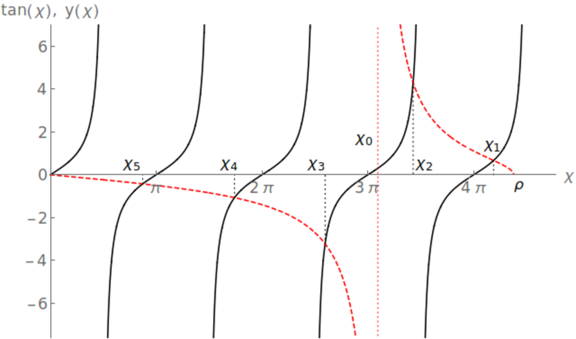
Figure 1: Graphical solution of equation (66), where the functions $\tan\chi$ and $y(\chi)$ are shown by solid (black) and dashed (red) curves, respectively. Five roots $\chi_{1},\ldots,\chi_{5}$ have been obtained as a result of intersecting these functions. Here $\rho=13.7$ and the function $y(\chi)$ has one infinite discontinuity at point $\chi=\chi_{0}$.

At the other end $\chi=\rho$, as follows from equations (68) and (69), we have $C_{1}\to+\,\infty$ and $C_{2}\to$ const. Then from equation (66) one can conclude that in the vicinity of the point $\chi=\rho$, the function $y(\chi)$ is positive. Since $C_{0}>0$ on the whole interval $(0,\rho)$ and the signs of the function $y(\chi)$ in the vicinity of the ends $\chi=0$ and $\chi=\rho$ are opposite, the denominator of $y(\chi)$ has one zero. Therefore the function $y(\chi)$ has an infinite discontinuity at the point $\chi_{0}=\rho/\sqrt{2}$ as shown in figure 1. On the interval $(0,\chi_{0})$, the function $y(\chi)$ is negative and positive on the interval $(\chi_{0},\rho)$.

For the double-well (DW) form of potential (21), some additional points of infinite discontinuity can appear and they will be located to the right of the point $\chi_{0}$. This follows from equations (71) because at the point $\chi=l_{1}\sqrt{V_{2}-V_{1}}$ (if $V_{1}\leq V_{2}$) or $\chi=l_{2}\sqrt{V_{1}-V_{2}}$ (if $V_{2}\leq V_{1}$), the parameter $\zeta$ changes from imaginary to real values. Therefore the points of infinite discontinuity can appear on the intervals $l_{1}\sqrt{V_{2}-V_{1}}<\chi<\rho_{1}$ (if $V_{1}\leq V_{2}$) or $l_{2}\sqrt{V_{1}-V_{2}}<\chi<\rho_{2}$ (if $V_{2}\leq V_{1}$). In the limit as $\rho$ approaches the origin, the function $y(\chi)$ is negative on some interval $0<\chi<\chi_{0}$, where $\chi_{0}$ is the point of the first infinite discontinuity that also approaches the origin as $\rho\to 0$. Therefore for sufficiently small $\rho$, only one root of equation (66) survives and it will be located on the interval $(0,\pi/2)$. Hence equation (66) can admit in the $\rho\to 0$ limit only one root.

Note that during the realization of point interactions in the squeezing limit, the inequality $V_{1}(l_{1})\leq V_{2}(l_{2})$ [or $V_{2}(l_{2})\leq V_{1}(l_{1})$] must be retained, independently on $l_{1}$ and $l_{2}$ , because the parameter $\zeta$ in equations (66)–(69) must be either real or imaginary during the whole squeezing procedure. Indeed, this is true because in definition (71) for the DW case we have $\chi^{2}-\rho_{1}^{2}-V_{2}l_{1}^{2}=\chi^{2}-(V_{1}-V_{2})l_{1}^{2}$ and similarly $\chi^{2}-\rho_{2}^{2}-V_{1}l_{2}^{2}=\chi^{2}+(V_{1}-V_{2})l_{2}^{2}$ , so that the sign of the difference $V_{1}-V_{2}$ is preserved during the whole squeezing process.

Thus, for a finite double-layer structure, there exists a finite number $N$ of solutions $\chi_{1}$, $\ldots,\chi_{N}$ to equation (66) as illustrated by figure 1. In the limit as $\rho\to 0$, only the root $\chi_{N}$ survives. However, in spite of the existence of this root that approaches $\rho\to 0$, a non-trivial limit of the level $\kappa_{N}$, which could follow from the $N$th equation (74), in general does not exist. Similarly, in the other limit as $\rho\to$ const. $\neq 0$, it follows from equations (74) that only the root $\chi_{1}$ can survive if it approaches $\rho$. Therefore in both these cases, $\sqrt{\rho^{2}-\chi^{2}}\to 0$. Taking for account this behavior, equations (66)–(69) can asymptotically be replaced by

$${\chi\tan\chi+\zeta\tan\bar{\zeta}\over\sqrt{\rho^{2}-\chi^{2}}}\simeq 2-\left({\chi\over\zeta}+{\zeta\over\chi}-{\chi\,\zeta\,r\over l\sqrt{\rho^{2}-\chi^{2}}}\right)\tan\chi\tan\bar{\zeta}.$$ (76)

Because of the denominator, the left-hand side of this equation diverges as $\chi\to\rho$ and therefore we must impose the condition

$$\chi\tan\chi+\zeta\tan\bar{\zeta}=0.$$ (77)

This is the necessary condition for the equation (76) to be well-defined in the limit as $\chi\to\rho$. Coming back, according to equations (70)–(72), to the variables $k_{j}l_{j}$, $j=1,2$, one immediately finds that equation (77) reduces to resonance sets (57). The last term in the right-hand side of equation (76) may be finite as $\chi\to\rho$ if $r\to 0$ sufficiently fast. Setting additionally $l\sqrt{\rho^{2}-\chi_{N}^{2}}=\kappa_{N}$ if $\rho\to 0$ and $l\sqrt{\rho^{2}-\chi_{1}^{2}}=\kappa_{1}$ if $\rho\to\mbox{const.}\neq 0$, we get from equation (76) the same asymptotic representation $\kappa_{i}\simeq\Delta/(z_{1}+z_{2})$ with $i=1$ or $N$, where $\Delta$, $z_{1}$ and $z_{2}$ are defined by equations (49) and (50). Therefore, only on resonance sets (57), $\kappa_{1}$ or $\kappa_{N}$ converges to the bound state level $\kappa$ defined by equations (63). In summary, we conclude that the convergence of the multiple bound states $\kappa_{1},\ldots,\kappa_{N}$ to a single level $\kappa$ proceeds in the two ways: (i) in the case if $\rho\to 0$, the lowest energy level $\kappa_{N}\to\kappa$, whereas the rest of higher levels tend to zero, i.e.,

$$\kappa_{1}\to 0,~{}\kappa_{2}\to 0,\ldots,\kappa_{N-1}\to 0,~{}~{}\kappa_{N}\to\kappa>0,$$ (78)

(ii) contrary, in the case if $\rho\to\mbox{const.}\neq 0$, the highest energy level $\kappa_{1}\to\kappa$, while the rest lower levels escape to infinity, resulting in the convergence sequence

$$\kappa_{1}\to\kappa>0,~{}~{}~{}\kappa_{2},\ldots\kappa_{N}\to\infty.$$ (79)

6 Three-scale power-connecting parametrization of a double-layer potential

Thus, for realizing both separated and non-separated point interactions from a double-layer structure, the layer widths $l_{1},\,l_{2}$ and the distance between the layers $r$ in potential (21) are required to shrink to the origin $x=0$ along any path $\gamma=\{l_{1},l_{2},r\}\in\Gamma$, while $V_{1}$ and $V_{2}$ belonging to the ${\cal G}$-sets must tend to infinity. The $\Gamma$-space is interpreted as a pencil of paths that approach the origin obeying the limit conditions for the expressions listed in (29) and (30). Only on those paths belonging to the pencil $\Gamma$, at which the resonance $X$- and $Y$-sets are defined by equations (45) and (57), the non-separated point interactions are materialized, while beyond these sets the interactions are separated fulfilling boundary conditions (31). Moreover, on the resonance sets, the scattering data $a(k)$ and $b(k)$ as well as bound states are shown to exist as well-defined quantities. From a visualization point of view, in order to demonstrate the convergence of the discrete spectrum and the behavior of the wave function in a squeezed limit, it would be convenient to parametrize potential (21) and the paths $\gamma$’s via an appropriately chosen one squeezing parameter, which could connect all the potential parameters $V_{1}$, $V_{2}$, $l_{1}$, $l_{2}$ and $r$. There are various possible parametrizations of these parameters, each of which being a subset of the ${\cal G}$-sets and the $\Gamma$-space. To this end, we choose here a power-connecting parametrization used in [55, 62, 63] for other purposes. It couples three positive powers $\mu$, $\nu$ and $\tau$ via a dimensionless squeezing parameter $\varepsilon>0$ as follows

$$V_{1}=\varepsilon^{-\mu}h_{1}\,,~{}V_{2}=\varepsilon^{-\nu}h_{2}\,,~{}l_{1}=\varepsilon d_{1}\,,l_{2}=\varepsilon^{1-\mu+\nu}d_{2}\,,~{}r=\varepsilon^{\tau}c.$$ (80)

Here the coefficients $h_{j}\in{\mathbb{R}}$, $j=1,2$, are characteristic quantities of the system, so that they may be called the layer intensities (or amplitudes). In the following, we denote potential (21) parametrized by equations (80) as $V_{\varepsilon}(x)$. Clearly, the dependence of $V_{1}$ and $V_{2}$ on $l_{1}$ and $l_{2}$ can be expressed from (80) explicitly using a power gymnastics. Then, for the limits $|V_{j}(l_{j})|^{1/2}l_{j}\to c_{j}\geq 0$, $j=1,2$, to be fulfilled, the conditions on the parameters $\mu$ and $\nu$ can be found and they will be given below.

6.1 Existence set for the distribution $\delta^{\prime}(x)$

The explicit representation (80) allows us to define in the $\{\mu,\nu,\tau\}$-space the set where potential (21) converges to $\delta^{\prime}(x)$ in the sense of distributions. Thus, using the fast variable $\xi=x/\varepsilon$, for any test function $\varphi(x)\in C_{0}^{\infty}({\mathbb{R}})$, we have

$$\langle V_{\varepsilon}(x)\,|\,\varphi(x)\rangle=\int_{0}^{l_{1}+l_{2}+r}V_{\varepsilon}(x)\varphi(x)dx$$

$$=\varepsilon\left[h_{1}\varepsilon^{-\mu}\int_{0}^{d_{1}}\varphi(\varepsilon\xi)d\xi+h_{2}\varepsilon^{-\nu}\int_{d_{1}+c\,\varepsilon^{\tau-1}}^{d_{1}+d_{2}\,\varepsilon^{\nu-\mu}+c\,\varepsilon^{\tau-1}}\varphi(\varepsilon\xi)d\xi\right].$$ (81)

Expanding next $\varphi(\varepsilon\xi)=\varphi(0)+\varepsilon\xi\varphi^{\prime}(0)+(\varepsilon\xi)^{2}\varphi^{\prime\prime}(0)/2+{\cal O}(\varepsilon^{3})$, we compute

$$\!\!\!\!\!\!\!\!\!\langle V_{\varepsilon}(x)\,|\,\varphi(x)\rangle = \varepsilon^{1-\mu}\,(h_{1}d_{1}+h_{2}d_{2})\,\varphi(0)+{\varepsilon^{2-\mu}\over 2}\left[h_{1}d_{1}^{2}+\varepsilon^{\nu-\mu}h_{2}d_{2}^{2}\right.$$ (82)

$$+ \left.2h_{2}d_{2}\left(d_{1}+\varepsilon^{\tau-1}c\right)\right]\varphi^{\prime}(0)+{\cal O}(\varepsilon^{3-\mu})+{\cal O}(\varepsilon^{3-3\mu+2\nu})$$

$$+ {\cal O}(\varepsilon^{\tau+2-\mu+\nu})+{\cal O}(\varepsilon^{\tau+2-2\mu+2\nu})+{\cal O}(\varepsilon^{2\tau+1-\mu+\nu}).$$

The first term in this expansion diverges if $\mu>1$. However, it cancels out under the condition

$$h_{1}d_{1}+h_{2}d_{2}=0$$ (83)

as a necessary condition for the existence of $\delta^{\prime}(x)$. It can be fulfilled only either on the second (WB structure) or on the fourth (BW structure) quadrant of the $\{h_{1},h_{2}\}$-plane at given widths $d_{1}$ and $d_{2}$. For the analysis of the second term in expansion (82), in the $\{\mu,\nu,\tau\}$-space we single out the trihedral angle formed by vertex $P_{1}$ , edges $K_{1}\,,\,L_{1}\,,\,N_{1}$ and planes $Q_{1}\,,\,O_{1}\,,\,S_{1}$ , with interior space set $I_{1}$ , which are defined by the equations

$$\begin{array}[]{lllllll}P_{1}&:=&\{\mu=\nu=2,\,\tau=1\},\\ K_{1}&:=&\{1<\mu<2,\,\nu=2(\mu-1),\,\tau=\mu-1\},\\ L_{1}&:=&\{\mu=2,\,2<\nu<\infty,\,\tau=1\},\\ N_{1}&:=&\{\mu=\nu=2,\,1<\tau<\infty\},\\ Q_{1}&:=&\{1<\mu<2,\,\nu=2(\mu-1),\,\mu-1<\tau<\infty\},\\ O_{1}&:=&\{\mu=2,\,2<\nu<\infty,\,1<\tau<\infty\},\\ S_{1}&:=&\{1<\mu<2,\,2(\mu-1)<\nu<\infty,\,\tau=\mu-1\},\\ I_{1}&:=&\{1<\mu<2,\,2(\mu-1)<\nu<\infty,\,\mu-1<\tau<\infty\}\end{array}$$ (84)

and illustrated by figure 2.

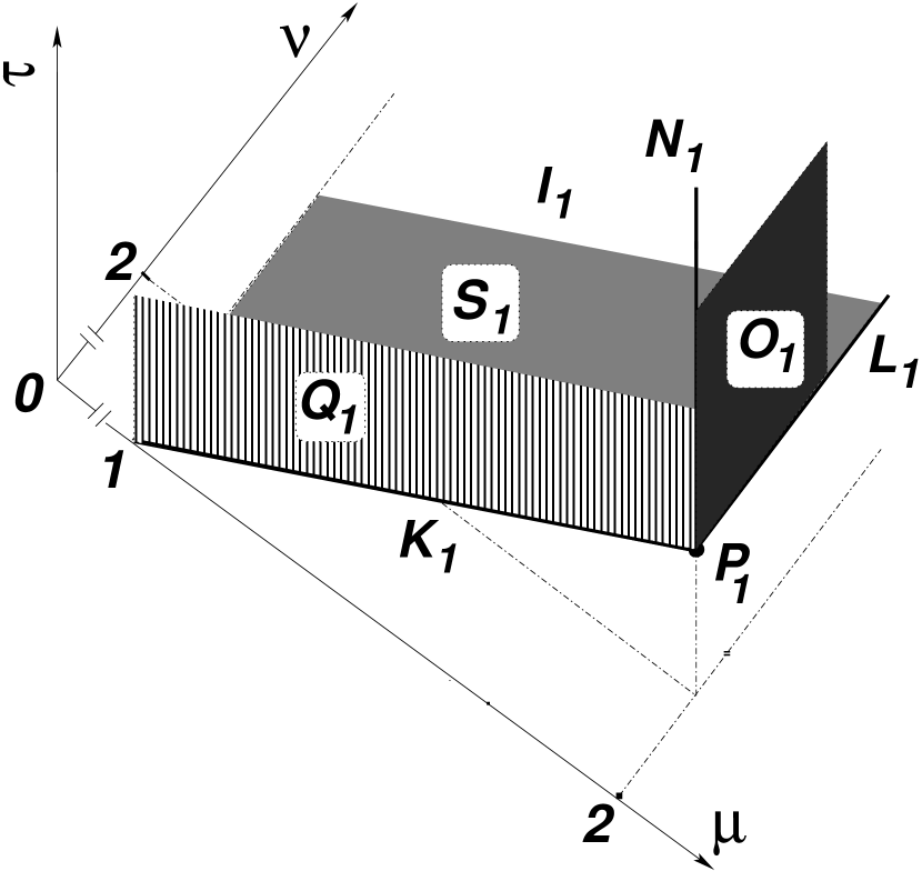
Figure 2: The $S_{\delta^{\prime}}$-surface of the existence of the distribution $\delta^{\prime}(x)$ obtained from a double-layer structure. The elements of this surface are defined by equations (84).

In the set $I_{1}$ , the second term in expansion (82) vanishes as $\varepsilon\to 0$, whereas beyond the angle it diverges in this limit. It is remarkable that on the angle surface $S_{\delta^{\prime}}:=P_{1}\cup K_{1}\cup L_{1}\cup N_{1}\cup Q_{1}\cup O_{1}\cup S_{1}$ the second term has finite limit values. The remainder terms in expansion (82) tend to zero in the limit as $\varepsilon\to 0$ because all the powers therein are positive if they are considered on the surface $S_{\delta^{\prime}}$. Therefore, with taking for account equation (83), we have

$$\langle V_{\varepsilon}(x)\,|\,\varphi(x)\rangle\simeq-\,{h_{1}d_{1}\over 2}\varepsilon^{2-\mu}\left(d_{1}+\varepsilon^{\nu-\mu}d_{2}+2\varepsilon^{\tau-1}c\right)\varphi^{\prime}(0).$$ (85)

It follows from this asymptotic representation that the potential $V_{\varepsilon}(x)$ converges to $\gamma\delta^{\prime}(x)$ in the sense of distributions if condition (83) holds true. Here, the strength constant $\gamma$ is the set function defined by

$$\gamma={h_{1}d_{1}\over 2}\left\{\begin{array}[]{lllllll}d_{1}+d_{2}+2c\!\!&\mbox{at point}~{}\,P_{1}\,,\\ d_{2}+2c&\mbox{on line}~{}K_{1}\,,\\ d_{1}+2c&\mbox{on line}~{}L_{1}\,,\\ d_{1}+d_{2}&\mbox{on line}~{}N_{1}\,,\\ d_{2}&\mbox{on area}~{}Q_{1}\,,\\ d_{1}&\mbox{on area}~{}O_{1}\,,\\ 2c&\mbox{on area}~{}S_{1}\,.\end{array}\right.$$ (86)

Thus, under condition (83), the surface $S_{\delta^{\prime}}$ separates in the $\{\mu,\nu,\tau\}$-space the volume region $I_{1}$ of perfect transmission and the region of non-existence of point interactions.

6.2 Parametrized resonance sets and scattering data

The three-scale parametrization given by equations (80) allows us to realize the geometric diagram in the $\{\mu,\nu,\tau\}$-space (depicted in figure 3), where the sets for all the four cases of the $\varepsilon\to 0$ limits of the arguments $k_{1}l_{1}$ and $k_{2}l_{2}$ , i.e., (i) $k_{1}l_{1}\to\sigma_{1}\neq 0$ and $k_{2}l_{2}\to\sigma_{2}\neq 0$, (ii) $k_{1}l_{1}\to 0$ and $k_{2}l_{2}\to\sigma_{2}\neq 0$, (iii) $k_{1}l_{1}\to\sigma_{1}\neq 0$ and $k_{2}l_{2}\to 0$, (iv) $k_{1}l_{1}\to 0$ and $k_{2}l_{2}\to 0$, can be represented. The $\varepsilon\to 0$ limits of $k_{j}l_{j}$’s, $j=1,2$, define the four sets on the $\{\mu,\nu\}$-plane section, on which

$$k_{1}l_{1}\simeq\varepsilon^{1-\mu/2}\sqrt{-h_{1}}\,d_{1}\,~{}~{}\mbox{and}~{}~{}\,k_{2}l_{2}\simeq\varepsilon^{1-\mu+\nu/2}\sqrt{-h_{2}}\,d_{2}\,.$$ (87)

The other eight limits $f_{j}$, $\eta_{j}$, $g_{j}$, $\beta_{j}$ ($j=1,2$) defined by equations (44) and (56) determine the power $\tau$ as a function of $\mu$ and $\nu$. Their asymptotic representation is

$$f_{1} \simeq k_{1}r\simeq\varepsilon^{\tau-\mu/2}\sqrt{-h_{1}}\,c,~{}~{}f_{2}\simeq k_{2}r\simeq\varepsilon^{\tau-\nu/2}\sqrt{-h_{2}}\,c,$$

$$\eta_{j} \simeq k_{j}^{2}l_{j}r\simeq-\,\varepsilon^{\tau-\mu+1}h_{j}d_{j}c$$ (88)

for the resonance sets $X=\{X_{11},X_{01},X_{10},X_{00}\}$ and

$$g_{1} \simeq k_{1}r^{1/2}\simeq\varepsilon^{(\tau-\mu)/2}\sqrt{-h_{1}c},~{}~{}g_{2}\simeq k_{2}r^{1/2}\simeq\varepsilon^{(\tau-\nu)/2}\sqrt{-h_{2}c},$$

$$\beta_{j} \simeq k_{j}^{2}l_{j}r^{1/2}\simeq-\,\varepsilon^{\tau/2-\mu+1}h_{j}d_{j}c^{1/2}$$ (89)

for the resonance sets $Y=\{Y_{11},Y_{01},Y_{10},Y_{00}\}$. Hence asymptotic representation (87)–(89) admits either finite limits

$$\begin{array}[]{ll}\sigma_{j}=\sqrt{-h_{j}}\,d_{j},~{}~{}f_{j}=\sqrt{-h_{j}}\,c,~{}~{}\eta_{j}=-\,h_{j}d_{j}c&\mbox{for}~{}~{}X\mbox{-sets},\\ \sigma_{j}=\sqrt{-h_{j}}\,d_{j},~{}~{}g_{j}=\sqrt{-h_{j}c}\,,~{}~{}\beta_{j}=-\,h_{j}d_{j}c^{1/2}&\mbox{for}~{}~{}Y\mbox{-sets},\end{array}$$ (90)

or zero. Therefore equations (45) together with relations (90) for $X$-sets are reduced to

$$\!\!\!\!\!\!\!\!\!\left.\begin{array}[]{llll}X_{11}:\cot(\sqrt{-h_{1}}\,d_{1})/\sqrt{-h_{1}}+\cot(\sqrt{-h_{2}}\,d_{2})/\sqrt{-h_{2}}\\ X_{01}:-1/h_{1}d_{1}+\cot(\sqrt{-h_{2}}\,d_{2})/\sqrt{-h_{2}}\\ X_{10}:\cot(\sqrt{-h_{1}}\,d_{1})/\sqrt{-h_{1}}-1/h_{2}d_{2}\\ X_{00}:-1/h_{1}d_{1}-1/h_{2}d_{2}\end{array}\right\}=c~{}~{}\left.\begin{array}[]{llll}\mbox{at}~{}~{}P_{1}\,,\\ \mbox{on}~{}~{}K_{1}\,,\\ \mbox{on}~{}~{}L_{1}\,,\\ \mbox{on}~{}~{}S_{1}\,.\end{array}\right.$$ (91)

Inserting next values (90) into equations (46), we get the element $\theta$ and consequently the scattering data $a$ and $b$ given by equations (47) that do not depend on $k$.

Similarly, inserting values (90) for $Y$-sets into equations (57), we obtain the explicit representation of the resonance sets:

$$\!\!\!\!\!\!\!\!\!\!\!\!\left.\begin{array}[]{llll}Y_{11}:\sqrt{-h_{1}}\tan(\sqrt{-h_{1}}\,d_{1})\!+\sqrt{-h_{2}}\tan(\sqrt{-h_{2}}\,d_{2})\!\!\!\\ Y_{01}:h_{1}d_{1}-\sqrt{-h_{2}}\tan(\sqrt{-h_{2}}\,d_{2})\!\!\!\\ Y_{10}:\sqrt{-h_{1}}\tan(\sqrt{-h_{1}}\,d_{1})-h_{2}d_{2}\!\!\!\\ Y_{00}:h_{1}d_{1}+h_{2}d_{2}\!\!\!\end{array}\right\}=0~{}~{}\mbox{on}~{}\left\{\begin{array}[]{llll}P_{2}\cup N_{2}\,,\\ K_{2}\cup Q_{2}\,,\\ L_{2}\cup O_{2}\,,\\ S_{2}\cup I_{2}\,,\end{array}\!\!\right.~{}~{}$$ (92)

where the sets

$$\begin{array}[]{lllllll}P_{2}&:=&\{\mu=\nu=\tau=2\},\\ K_{2}&:=&\{1<\mu<2,\,\nu=\tau=2(\mu-1)\},\\ L_{2}&:=&\{\mu=2,\,2<\nu<\infty,\,\tau=2\},\\ N_{2}&:=&\{\mu=\nu=2,\,2<\tau<\infty\},\\ Q_{2}&:=&\{1<\mu<2,\,\nu=2(\mu-1),\,\mu-1<\tau<\infty\},\\ O_{2}&:=&\{\mu=2,\,2<\nu<\infty,\,2<\tau<\infty\},\\ S_{2}&:=&\{1<\mu<2,\,2(\mu-1)<\nu<\infty,\,\tau=2(\mu-1)\},\\ I_{2}&:=&\{1<\mu<2,\,2(\mu-1)<\nu<\infty,\,2(\mu-1)<\tau<\infty\}\end{array}$$ (93)

form the second trihedral angle with vertex $P_{2}$, edges $K_{2}$, $L_{2}$, $N_{2}$ and planes $Q_{2}$, $O_{2}$, $S_{2}$, including interior space set $I_{2}$ (see figure 3). Inserting now values (90) for the $Y$-sets into equations (58) and (59), we obtain the expressions for the elements $\theta$ and $\alpha$ which make sense only in the second trihedral angle on the resonance $Y$-sets, being the solutions to equations (92). Note that these solutions (the resonance $Y_{11}$-, $Y_{01}$-, $Y_{10}$-surfaces and $Y_{00}$-plane) appear to be the limits of the corresponding $X$-surfaces as formally $c\to 0$ [compare equations (91) and (92)].

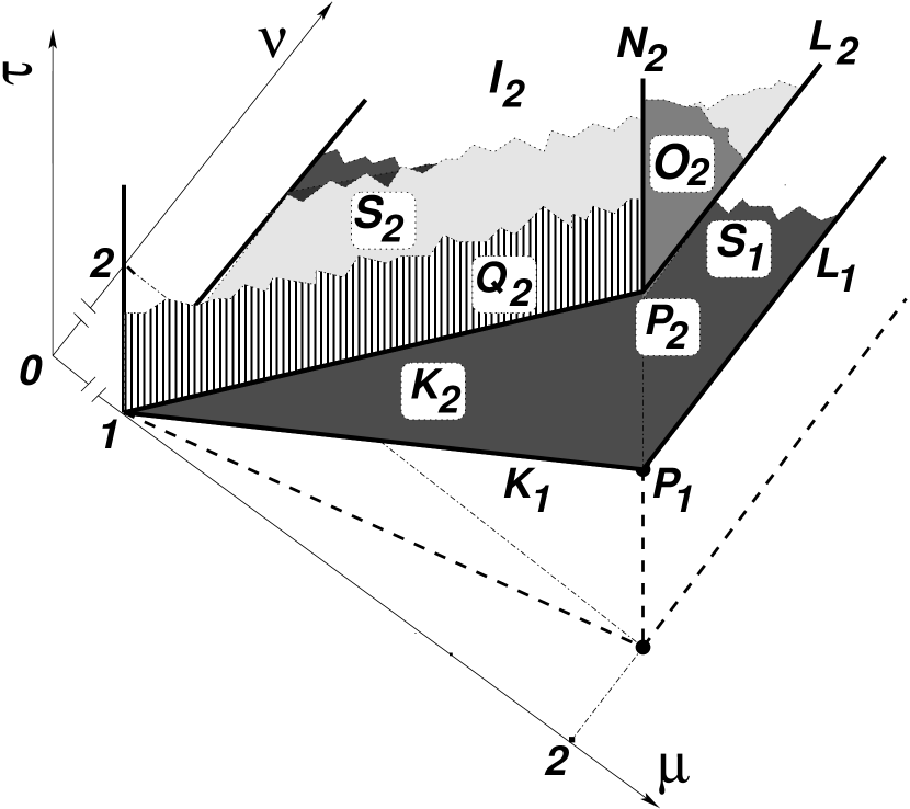
Figure 3: Sets defined by equations (84) and (93) on which the point interactions of the first (with subscript ‘1’) and the second (with subscript ‘2’) types are realized. The sets of the first type are found on the plane $\{1<\mu\leq 2,~{}2(\mu-1)\leq\nu<\infty,~{}\tau=\mu-1\}$, whereas the interactions of the second type in the space $\{1<\mu\leq 2,~{}2(\mu-1)\leq\nu<\infty,~{}2(\mu-1)\leq\tau<\infty\}$.

According to asymptotic representation (89) with limit values (90) for the $Y$-sets, the elements $\theta$ given by the first formulas (58) and $\alpha$ defined by equations (59) are reduced to

$$\theta=\left\{\begin{array}[]{llll}\cos(\sqrt{-\,h_{1}}\,d_{1})/\cos(\sqrt{-\,h_{2}}\,d_{2})&\\ 1/\cos(\sqrt{-\,h_{2}}\,d_{2})&\\ \cos(\sqrt{-\,h_{1}}\,d_{1})&\\ 1&\\ \end{array}\right.~{}~{}~{}\mbox{on}~{}~{}~{}\left\{\begin{array}[]{llll}~{}P_{2}\cup N_{2}\,,&\\ ~{}K_{2}\cup Q_{2}\,,&\\ ~{}L_{2}\cup O_{2}\,,&\\ ~{}S_{2}\cup I_{2}\,,&\end{array}\right.$$ (94)

$$\!\!\!\!\!\!\!\!\!\alpha=h_{1}h_{2}\,c\left\{\begin{array}[]{llll}(1/\sqrt{-h_{1}}\,\sqrt{-h_{2}}\,)\sin(\sqrt{-\,h_{1}}\,d_{1})\sin(\sqrt{-\,h_{2}}\,d_{2})&\mbox{at}~{}P_{2}\,,\\ (d_{1}/\sqrt{-h_{2}}\,)\sin(\sqrt{-\,h_{2}}\,d_{2})&\mbox{on}~{}K_{2}\,,\\ (d_{2}/\sqrt{-h_{1}}\,)\sin(\sqrt{-\,h_{1}}\,d_{1})&\mbox{on}~{}L_{2}\,,\\ d_{1}d_{2}&\mbox{on}~{}S_{2}\end{array}\right.$$ (95)

and $\alpha=0$ in the space region $Q_{2}\cup O_{2}\cup N_{2}\cup I_{2}$ .

Thus, equations (91) and (92) are the conditions at which the scattering data $a(k)$ and $b(k)$ are well-defined quantities. At fixed $d_{1}$ and $d_{2}\,,$ the solutions of these equations can be represented on the $\{h_{1},h_{2}\}$-plane (more precisely, on the WB, DW and BW quadrants) in the form of curves, similarly to those depicted in the corresponding figures of work [55] (see figure 2 for $X_{00}\,,$ and $Y_{00}$ , figure 3 for $X_{01}\,,$ and $Y_{01}$ , figure 4 for $X_{10}$ and $Y_{10}$ , figure 5 for $X_{11}$ and $Y_{11}$ therein). The cancellation of divergences of the first type results in the existence of resonance $X$-sets (91) in the section plane $\tau=\mu-1$, whereas the cancellation of the second type leads to the existence of resonance $Y$-sets in the space region $\tau\geq 2(\mu-1)$.

From the whole family of point interactions, which are realized on the resonance sets described by equations (91) and (92), one can single out the interactions with additional condition (83) for the existence of the distribution $\delta^{\prime}(x)$. Therefore the whole family realized in general from both the BW and DW configurations of potential (21) can be referred to as generalized $\delta^{\prime}$-potentials, while the subfamily restricted by constraint (83) distributional ones. The name ‘$\delta^{\prime}$-potentials’ (both generalized and distributional) comes from the fact that the element $\theta(k)$ determined by equations (46) and (58) on the $X$- and $Y$-sets except for the set $Y_{00}$ does not identically equal the unity [14]. The point interaction with $\theta(k)=1$ [see the last equations in (58) and (94)] may be called a generalized $\delta$-potential because the corresponding profile of potential (21) has no a $\delta(x)$ limit as $\varepsilon\to 0$.

6.3 Bound state level $\kappa$

Inserting expressions (94) and (95) into the formula for the level $\kappa$ in (62), on resonance sets (92), the level $\kappa$ is

$$\kappa|_{P_{2}\times Y_{11}} = -\,{h_{1}c\tan^{2}(\sqrt{-\,h_{1}}\,d_{1})\over\cos^{-2}(\sqrt{-\,h_{1}}\,d_{1})+\cos^{-2}(\sqrt{-\,h_{2}}\,d_{2})}$$

$$= -\,{h_{2}c\tan^{2}(\sqrt{-\,h_{2}}\,d_{2})\over\cos^{-2}(\sqrt{-\,h_{1}}\,d_{1})+\cos^{-2}(\sqrt{-\,h_{2}}\,d_{2})}\,,$$

$$\kappa|_{K_{2}\times Y_{01}} = {(h_{1}d_{1})^{2}c\over 1+\cos^{-2}(\sqrt{-\,h_{2}}\,d_{2})}={h_{2}c\over 2(h_{1}d_{1})^{-2}h_{2}-1}\,,$$

$$\kappa|_{L_{2}\times Y_{10}} = {(h_{2}d_{2})^{2}c\over 1+\cos^{-2}(\sqrt{-\,h_{1}}\,d_{1})}={h_{1}c\over 2(h_{2}d_{2})^{-2}h_{1}-1}\,,$$

$$\kappa|_{S_{2}\times Y_{00}} = \frac{1}{2}(h_{1}d_{1})^{2}c=\frac{1}{2}(h_{2}d_{2})^{2}c\,.$$ (96)

6.4 Convergence of multiple bound state levels to a squeezed single value

Parametrization (80) as a particular pathway of materializing point interactions from a double-layer system, allows us to control explicitly the behavior of all the roots $\chi_{1},\dots,\chi_{N}$ as the solutions of equation (66) with (67)–(69), under the shrinking of the system to a point. Accordingly, due to relations (74), one can observe the behavior of bound state levels $\kappa_{1},\ldots,\kappa_{N}$. In particular, one can establish which of the lateral levels $\kappa_{1}$ or $\kappa_{N}$ converges to a single level $\kappa$. Contrary to the case with a single rectangular well, here the convergence is available only on the resonance $Y$-sets defined by equations (92). This means that the finite limit values for the bound state $\kappa$ can be obtained if the powers $\mu$, $\nu$ and $\tau$ are found on the plane $\tau=2(\mu-1)$, i.e., on the set $P_{2}\cup K_{2}\cup L_{2}\cup S_{2}$, on one side, and on the other side, the system parameters $h_{1},$ $d_{1},$ $h_{2},$ $d_{2}$ must obey equations (92), while $c>0$ may be arbitrary.

Equation (66) has been derived for the variable $\chi$ that corresponds to the well (in the BW case) or to the deepest well (in the DW case). Therefore there are two cases: $V_{1}<0$, $V_{2}\in{\mathbb{R}}$, $V_{1}\leq V_{2}$ and $V_{1}\in{\mathbb{R}}$, $V_{2}<0$, $V_{1}\geq V_{2}$. The parameters $\rho$ as well as $\zeta$, $\bar{\zeta}$ and $t_{0}$ defined by equations (71)–(73) and involved into equations (67)–(69) are given explicitly in terms of $\mu,\nu,\tau$ and $\varepsilon$ as follows

$$\begin{array}[]{llll}\rho_{1}&=&\varepsilon^{1-\mu/2}|h_{1}|^{1/2}d_{1}\,,\\ \zeta_{1}&=&\left[\chi^{2}-\rho_{1}^{2}-\varepsilon^{2-\nu}h_{2}d_{1}^{2}\,\right]^{1/2},\\ \bar{\zeta}_{1}&=&\left[\varepsilon^{2(\nu-\mu)}(\chi^{2}-\rho_{1}^{2})(d_{2}/d_{1})^{2}-\varepsilon^{2(1-\mu)+\nu}h_{2}d_{2}^{2}\right]^{1/2},\\ t_{0,1}&=&\tanh\!\left[\varepsilon^{\tau-1}(c/d_{1})\sqrt{\rho_{1}^{2}-\chi^{2}}\,\right]\end{array}$$ (97)

if $V_{1}\leq V_{2}$ and

$$\begin{array}[]{llll}\rho_{2}&=&\varepsilon^{1-\mu+\nu/2}|h_{2}|^{1/2}d_{2}\,,\\ \zeta_{2}&=&\left[\chi^{2}-\rho_{2}^{2}-\varepsilon^{2-3\mu+2\nu}h_{1}d_{2}^{2}\,\right]^{1/2},\\ \bar{\zeta}_{2}&=&\left[\varepsilon^{2(\mu-\nu)}(\chi^{2}-\rho_{2}^{2})(d_{1}/d_{2})^{2}-\varepsilon^{2-\mu}h_{1}d_{1}^{2}\right]^{1/2},\\ t_{0,2}&=&\tanh\!\left[\varepsilon^{\tau-1+\mu-\nu}(c/d_{2})\sqrt{\rho_{2}^{2}-\chi^{2}}\,\right]\end{array}$$ (98)

if $V_{2}\leq V_{1}$. Note that one of the sets of equations (97) or (98) must be used during the squeezing procedure as $\varepsilon\to 0$, at least beginning from some small value $\varepsilon>0$. Which of these sets has to be applied, depends on the shape of the potential $V_{\varepsilon}(x).$ The configurations (i), (ii) and (iii) listed below cover all the possible situations for the existence of bound states. (i) WB profile ($h_{1}<0,\,h_{2}>0$): any $\mu$ and $\nu$, equations (97) to be used. (ii) BW profile ($h_{1}>0,\,h_{2}<0$): any $\mu$ and $\nu$, equations (98) to be used. (iii) DW profile ($h_{1}<0,\,h_{2}<0$): $h_{1}\leq h_{2}$ and $\mu=\nu$ or any $h_{1},\,h_{2}$ and $\mu>\nu$, equations (97) to be used; $h_{1}\geq h_{2}$ and $\mu=\nu$ or any $h_{1},\,h_{2}$ and $\mu<\nu$, equations (98) to be used.

Equations (97) and (98) are used for the graphical illustration as the finite number of bound state levels $\kappa_{i}$’s converges to a single level $\kappa$ given by analytic expressions (96). Plotting $\tan\chi$ and $y(\chi)$ as functions of $\chi$ on the interval $0<\chi<\rho$, expressed by equations (66)–(69) in which the parameters $\zeta$, $\bar{\zeta}$, $\rho$ and $t_{0}$ are given by one of equations (97) or (98), one can find the roots $\chi_{i}$’s located at the intersection of the functions $\tan\chi$ and $y(\chi)$ as shown in figure 1.

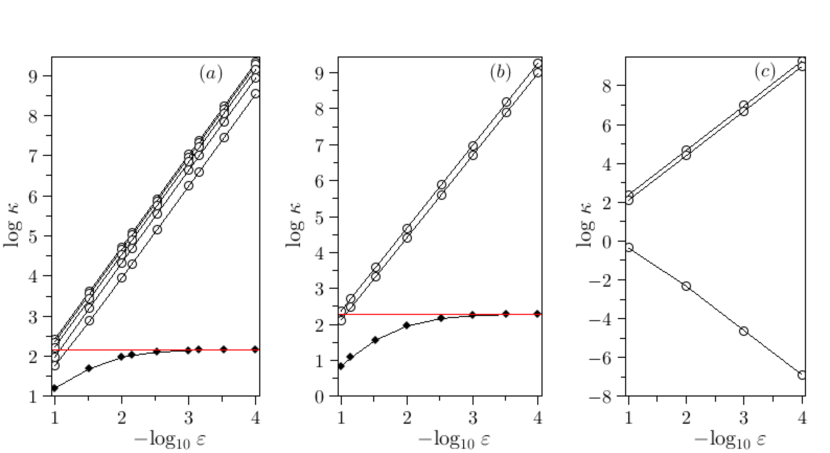
Figure 4: Convergence of bound state levels $\kappa_{i}$’s in the limit as $\varepsilon\to 0$ for the $\delta^{\prime}$-potentials realized from double-layer structure with parameters $h_{2}=-0.5$ eV and $c=20$ nm (for all cases below): (a) Generalized $\delta^{\prime}$-potential obtained from DW structure with parameters $h_{1}=-0.3$ eV, $d_{1}=2.1$ nm and $d_{2}=12.0$ nm obeying the first equation (92) for $P_{2}$. The $\{h_{1},d_{1},h_{2},d_{2}\}$-point with these parameter values lies on the 1st resonance surface of the $Y_{11}$-set. Figure 1 has been plotted for these values and the five levels $\kappa_{1},\ldots,\kappa_{5}$ as functions of $\varepsilon$ correspond to the five roots $\chi_{1},\ldots,\chi_{5}$ at $\varepsilon=1$. (b) Distributional $\delta^{\prime}$-potential materialized from BW structure with parameters $h_{1}=0.3$ eV, $d_{1}=10.1$ nm and $d_{2}=6.1$ nm fulfilling both the first equation (92) for $P_{2}$ and constraint (83). The $\{h_{1},d_{1},h_{2},d_{2}\}$-point with these parameter values lies on the intersection of the 2nd resonance surface of the $Y_{11}$-set and surface (83). For these values, there are three roots $\chi_{1},\,\chi_{2},\,\chi_{3}$ at $\varepsilon=1$. The solid (red) horizontal straight lines in (a) and (b) indicate the values for $\kappa$ given by the formulas for $\kappa|_{P_{2}\times Y_{11}}$ in (96). (c) Distributional $\delta^{\prime}$-potential obtained from BW profile with the same parameter values as in (b), but beyond the plane $\tau=2(\mu-1)$, lying on line $N_{2}$ with $\tau=3$. Here, there are also three roots at $\varepsilon=1$.

The parameter values for the numerical solution of equation (66) are chosen from the $\{h_{1},d_{1},h_{2},d_{2}\}$-space, which obey equations (92), and the parameter $c>0$ is supposed arbitrary. The powers $\mu$, $\nu$ and $\tau$ belong to the point $P_{2}$, one of the lines $K_{2}$ or $L_{2}$ and the plane $S_{2}$ defined by equations (93) and shown in figure 3. Having solved equation (66) at a given $\varepsilon>0$, then its solutions $\chi_{1},\ldots,\chi_{N}$ are inserted into equations (74) and the convergence of the levels $\kappa_{1},\ldots,\kappa_{N}$ is examined as $\varepsilon\to 0$. Note that the $\varepsilon\to 0$ limit values of $\kappa$ computed in this way must coincide with the analytic results given by equations (96). As follows from equations (97) and (98), in the limit as $\varepsilon\to 0$, either $\rho_{j}\to 0$ or $\rho_{j}\to|\sigma_{j}|=|h_{j}|^{1/2}d_{j}$, $j=1,2$. Below we describe the convergence of the levels $\kappa_{i}$’s on some sets of the $\{\mu,\nu,\tau\}$-space and indicate which of equations (97) or (98) has to be used in each case.

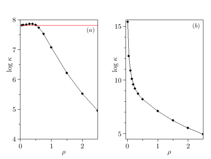
Figure 5: Convergence of the biggest (survived) bound state level $\kappa_{N}$ as $\rho=\varepsilon^{1/4}|h_{2}|^{1/2}d_{2}\to 0$ for point interactions realized from BW profile with parameters $h_{1}=|h_{2}|=0.5$ eV and $d_{1}=d_{2}=12$ nm: (a) Generalized $\delta$-potential obtained for the point $\{\mu=\nu=3/2,\,\tau=2(\mu-1)=1\}$ lying on plane $S_{2}$ . The solid (red) horizontal straight line indicates the value for $\kappa$ given by the formulas for $\kappa|_{S_{2}\times Y_{00}}$ in (96). (b) Point interaction of separated type (with full reflection) obtained for the same point on $S_{2}$, but beyond the resonance condition $h_{1}d_{1}=|h_{2}|d_{2}$. Here, $d_{1}=8$ nm, $d_{2}=12$ nm and $\kappa_{N}$ escapes to infinity.

Point $P_{2}$: At this point the convergence of $\kappa_{i}$, $i=1,\ldots,N$, is of type (79). The generalized $\delta^{\prime}$-potentials are materialized from the WB, DW and BW configurations. Equations (97) are used if $h_{1}\leq h_{2}\in{\mathbb{R}}$ and equations (98) if $h_{2}\leq h_{1}\in{\mathbb{R}}$. The distributional $\delta^{\prime}$-potentials are realized on the WB and BW quadrants. The convergence of $\kappa_{i}$’s to the squeezed value $\kappa$ obeying the first equation (96) is illustrated in figure 4: (a) for the generalized $\delta^{\prime}$-potential obtained from a DW profile and (b) for the distributional $\delta^{\prime}$-potential realized from a BW profile.

Line $N_{2}$: On this line located above the plane $\tau=2(\mu-1)$, the convergence of $\kappa_{i}$’s is also of type (79), except for the highest energy level $\kappa_{1}$, which converges to zero. In figure 4(c), the convergence of this type is plotted for the distributional $\delta^{\prime}$-potential obtained from a BW profile.

Plane $S_{2}$: On this plane the family of generalized $\delta$-potentials can be materialized if the system parameters satisfy the last equation in (92), which coincides with condition (83) for the existence of the distribution $\delta^{\prime}(x)$. Here the convergence is of type (78). The behavior of $\kappa_{i}$’s is shown in figure 5(a) for the biggest level $\kappa_{N}$ in the particular case: $\mu=\nu=3/2$, $h_{1}=-\,h_{2}$, $d_{1}=d_{2}$, where $\rho=\varepsilon^{1/4}|h_{2}|^{1/2}d_{2}$. From equations (74) one finds the asymptotic behavior of $\kappa_{N}$ in the limit as $\rho\to 0$ (or $\varepsilon\to 0$) as follows

$$\kappa_{N}=\rho^{-4}\,\sqrt{\rho^{2}-\chi_{N}^{2}}\,|h_{2}|^{2}d_{2}^{3}\,.$$ (99)

Using here equations (76) and (77), one can arrive at the last formula (96). Beyond the resonance $Y_{00}$-set, we have that $\kappa_{1}\to 0$, $\kappa_{2}\to 0$, $\ldots$, $\kappa_{N-1}\to 0$, but $\kappa_{N}\to\infty$ as shown in figure 5(b) for the level $\kappa_{N}$.

Line $K_{2}$: On this line the family of generalized $\delta^{\prime}$-potentials can be realized from the WB, DW and BW profiles on the resonance $Y_{01}$-set defined by the second equation (92). Equations (97) are used with $\rho_{1}\to 0$ for the WB and DW (if $h_{1}\leq h_{2}$ and $\mu=\nu$ or any $h_{1},\,h_{2}$ and $\mu>\nu$) profiles. Equations (98) are used with $\rho_{2}\to|h_{2}|^{1/2}d_{2}$ for the DW (if $h_{1}\geq h_{2}$ and $\mu=\nu$ or any $h_{1},\,h_{2}$ and $\mu<\nu$) and BW profiles. In the latter case, the distributional $\delta^{\prime}$-potentials are realized if condition (83) is imposed additionally. Here the convergence of type (79) takes place and the behavior of $\kappa_{i}$’s is similar to that shown in figure 4(b).

Line $L_{2}$: The situation on this line is similar to that as described for the line $K_{2}$. Here the family of generalized $\delta^{\prime}$-potentials can also be realized from the WB, DW and BW profiles, but now on the resonance $Y_{10}$-set defined by the third equation (92). Equations (97) are used with $\rho_{1}\to|h_{1}|^{1/2}d_{1}$ for the WB and DW (if $h_{1}\leq h_{2}$ and $\mu=\nu$ or any $h_{1},\,h_{2}$ and $\mu>\nu$) profiles. Equations (98) are used with $\rho_{2}\to 0$ for the DW (if $h_{1}\geq h_{2}$ and $\mu=\nu$ or any $h_{1},\,h_{2}$ and $\mu<\nu$) and BW profiles. In the former case, when equations (97) have to be used, the distributional $\delta^{\prime}$-potentials are realized if condition (83) is imposed additionally. Here the convergence of type (79) takes place and the behavior of $\kappa_{i}$’s is also similar to that shown in figure 4(b).

Thus, both generalized and distributional the $\delta^{\prime}$-potentials with non-zero bound states can be realized on the intersection of the plane $\tau=2(\mu-1)$ with the surface $S_{\delta^{\prime}}$, i.e., at the point $P_{2}$ and on the lines $K_{2}$ and $L_{2}$. The convergence of the levels $\kappa_{i}$’s for the point $P_{2}$ is of type (79), while on the lines $K_{2}$ and $L_{2}$ it can be of both types (78) and (79). Above these sets, on the line $N_{2}$ and on the planes $Q_{2}$ and $O_{2}$, the situation is quite similar, but here $\kappa_{N}\to 0$ in sequence (78) and $\kappa_{1}\to 0$ in sequence (79).

6.5 Convergence of wave functions in a squeezed limit

Parametrization (80) of potential (21) allows us to illustrate a pointwise convergence of solutions to equation (1) in the limit as $\varepsilon\to 0$, both for positive ($k^{2}>0$) and negative ($k^{2}=-\,\kappa^{2}$) energies. For a non-separated point interaction to be realized, the system parameters $h_{1},h_{2},d_{1},d_{2}$ must belong to one of the resonance $X$- or $Y$-sets described by equations (91) and (92). It is of interest to plot the wave functions on one of the $Y$-sets, because on these sets bound states are available. Therefore, as an appropriate example, we choose here a BW structure with the parameter values corresponding to the $Y_{11}$-set and determined by the first equation in (92).

Thus, on the basis of formula (32), the function $\phi_{1}(x)$ describing an incident plane wave (with a given $k$) from the right is plotted in figure 6 for three situations of shrinking a BW structure. The parameter values $h_{1},h_{2},d_{1},d_{2}$ satisfy the first equation in (92). For these values and the same three scales of squeezing the BW structure, the function $\phi_{1}(x)$, which describes a bound state, is plotted in figure 7 using the same equations (32) with $k={\rm i}\kappa$. The panels (c) in both figures clearly illustrate the appearance of a jump at $x=0$ that agrees with the first equation in (61), where $\theta$ is computed from the first equation in (94).

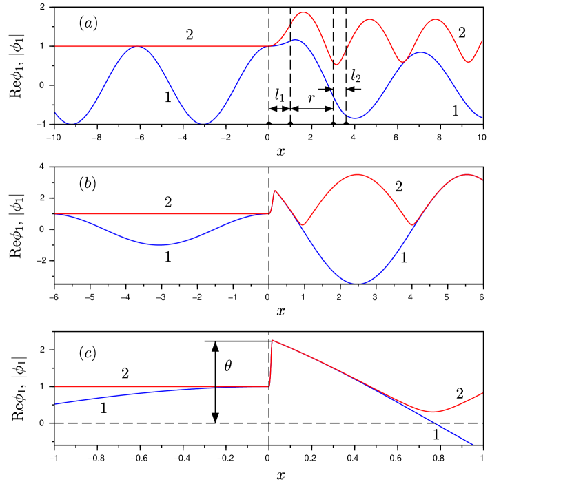
Figure 6: Profiles Re$\phi_{1}(x)$ (blue curves, 1) and $|\phi_{1}(x)|$ (red curves, 2) for (a) $\varepsilon=1$, (b) $\varepsilon=0.1$, (c) $\varepsilon=0.01$. The system parameter values are $h_{1}=0.5$ eV, $h_{2}=-0.5$ eV, $d_{1}=1.0$ nm, $d_{2}=0.6$ nm and $c=2.0$ nm. The energy of an incident particle is $k^{2}=0.4$ eV. In the squeezing limit [panel (c)], the jump of function $\phi_{1}(x)$ at $x=0$ reaches the value $\theta-1$ with $\theta=2.23$.

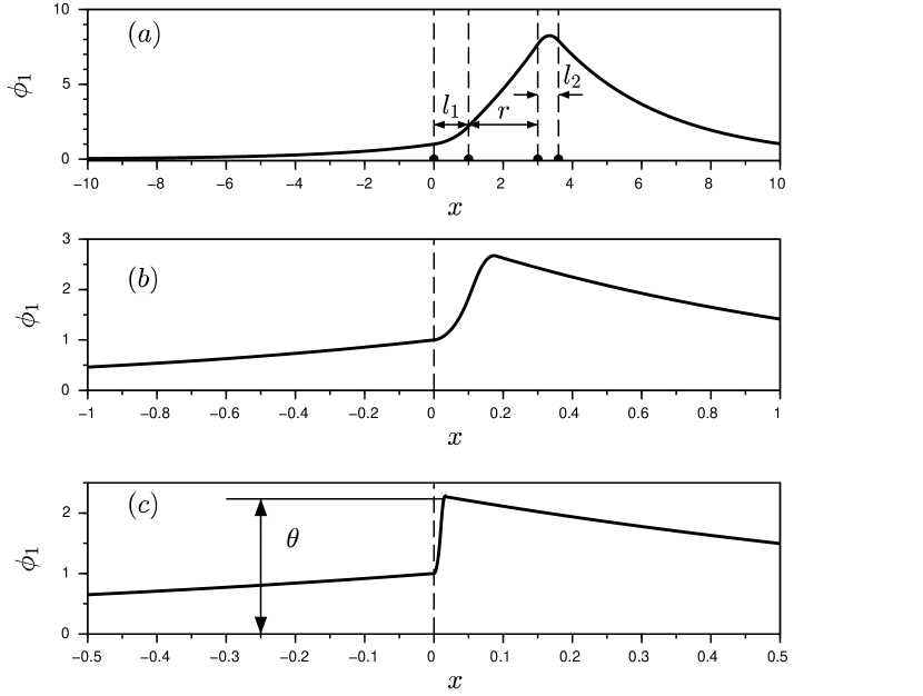
Figure 7: Eigenfunction $\phi_{1}(x)$ plotted for (a) $\varepsilon=1$, (b) $\varepsilon=0.1$, (c) $\varepsilon=0.01$. The system parameter values and $\theta$ are the same as in figure 6. Here the bound state levels are $\kappa=0.320$ ($\varepsilon=1$), $\kappa=0.773$ ($\varepsilon=0.1$), $\kappa=0.864$ ($\varepsilon=0.01$). The jump at $x=0$ illustrated by panel (c) is the same as in figure 6(c).

7 Concluding remarks

The procedure of squeezing a double-layer structure developed in this article is based on the simultaneous shrinking of the system parameters $l_{1},\,\l_{2}$ and $r$ to zero, which can be arranged in different ways. In this regard, the two families of the strength functions $V_{1}(l_{1})$ and $V_{2}(l_{2})$ have been defined by limit equations (43)–(44) and (55)–(56). These equations are expressed in terms of the limit characteristics $\sigma_{j}=\lim_{l_{j}\to 0}(k_{j}l_{j})$, $j=1,2$. The other eight limit characteristics involve the dependence on distance $r$: $f_{j},\,\eta_{j}\sim r^{-1}$ and $g_{j},\,\beta_{j}\sim r^{-1/2}$.

The squeezed limit of the scattering functions $a(k)$ and $b(k)$ is proven to be well-defined only if some constraints on the limit characteristics are imposed. These constraints are referred to as resonance sets, resulting from the two ways of the cancellation of divergences in the singular function $\Delta(k)$ given by formula (36). The first way is to put $\Delta(k)=0$, leading to the derivation of the resonance $X$-sets defined by equations (45). The second way requires that the squeezed limit of the function $\Delta(k)$ is a non-zero constant. In this way, the resonance $Y$-sets are defined by equations (57), on which the point interactions with non-trivial bound states can be realized.

As a particular example of the whole variety of the shrinking ways, we have chosen the three-scale parametrization [see equations (80)], where all the system parameters are connected through a dimensionless squeezing parameter $\varepsilon>0$. This connection, used in earlier publications [55, 62, 63], allows us to construct the geometric representation in the three-dimensional space of positive powers $\mu$, $\nu$ and $\tau$.

The three-scale power-connecting parametrization allows us to single out in the $\{\mu,\nu,\tau\}$-space the surface $S_{\delta^{\prime}}$ of the existence of the distribution $\delta^{\prime}(x)$ if condition (83) is imposed. This condition means that only barrier-well configurations are appropriate for the existence of $\delta^{\prime}(x)$. On the other hand, except for these configurations, double-well ones also participate in realizing the point interactions for which $a(k)$ and $b(k)$ are well-defined functions. In this article they are called generalized $\delta^{\prime}$-potentials.

There exists an ubiquitous opinion that the bound state energy levels for the Schrödinger equation (1) with a regularized potential $V_{\varepsilon}(x)$ escape to $-\,\infty$ as $V_{\varepsilon}(x)\to\beta\delta^{\prime}(x)$ in the sense of distributions ($\beta$ is a strength constant). In this article, it is shown that in general this is not true, except for the point interactions with an additional $\delta$-like potential [13, 31, 32, 61, 63, 64, 65, 66], where $V(x)=\alpha\delta(x)+\beta\delta^{\prime}(x)$, $\alpha<0$, $\beta\in{\mathbb{R}}$. On the basis of both the analytic arguments and the numerical computations, we prove that for the family of $\delta^{\prime}$-regularized potentials with certain configurations, a single bound energy level converges to a finite value, whereas the rest of energy levels escapes to $-\,\infty$. This is true in general for two families of point interactions, called in the present paper generalized $\delta$- and $\delta^{\prime}$-potentials, that cover their distributional analogues. The convergence of the multiple bound states under shrinking the finite-thickness double-layer structure to a point behaves according to one of sequences (78) or (79).

Acknowledgments

One of us (AVZ) acknowledges a partial support from the Department of Physics and Astronomy of the National Academy of Sciences of Ukraine (project No. 0117U000240). YZ acknowledges a partial support by the National Academy of Sciences of Ukraine Grant ‘Functional Properties of Materials Prospective for Nanotechnologies’ (project No. 0120U100858). Finally, we are indebted to both Referees for suggestions, resulting in the significant improvement of the paper.

References

References

- [1] Demkov Y N and Ostrovskii V N 1975 Zero-Range Potentials and Their Applications in Atomic Physics (Leningrad: Leningrad University Press)
- [2] Demkov Y N and Ostrovskii V N 1988 Zero-Range Potentials and Their Applications in Atomic Physics (New York: Plenum)
- [3] Albeverio S, Gesztesy F, Høegh-Krohn R and Holden H 2005 Solvable Models in Quantum Mechanics (With an Appendix by Pavel Exner) 2nd revised edn (Providence: RI: American Mathematical Society: Chelsea Publishing)
- [4] Albeverio S and Kurasov P 1999 Singular Perturbations of Differential Operators: Solvable Schrödinger-Type Operators (Cambridge: Cambridge University Press)
- [5] Berezin F A and Faddeev L D 1961 Sov. Math. Dokl. 2 372; translation from Dokl. Akad. Nauk SSSR 137 1011 (1961)
- [6] Kurasov P 1996 J. Math. Anal. Appl. 201 297
- [7] Albeverio S, Da̧browski L and Kurasov P 1998 Lett. Math. Phys. 45 33
- [8] Albeverio S and Nizhnik L 2003 Lett. Math. Phys. 65 27
- [9] Nizhnik L N 2003 J. Funct. Anal. Appl. 37 85
- [10] Nizhnik L N 2006 J. Funct. Anal. Appl. 40 74
- [11] Albeverio S, Cacciapuoti C and Finco D 2007 J. Math. Phys. 48 032103
- [12] Cacciapuoti C and Exner P 2007 J. Phys. A: Math. Theor. 40 F511
- [13] Gadella M, Negro J and Nieto L M 2009 Phys. Lett. A 373 1310
- [14] Brasche J F and Nizhnik L P 2013 Methods Funct. Anal. Topology 19 4
- [15] Kulinskii V L and Panchenko D Y 2015 Physica B 472 78
- [16] Nieto L M, Gadella M, Guilarte J M, Muñoz-Castañeda J M and Romaniega C 2017 J. Phys. Conf. Series 839 012007
- [17] Lange R-J 2012 J. High Energy Phys. JHEP11(2012)032
- [18] Lange R-J 2015 J. Math. Phys. 56 122105
- [19] Šeba P 1986 Rep. Math. Phys. 24 111
- [20] Exner P, Neidhardt H and Zagrebnov V A 2001 Commun. Math. Phys. 224 593
- [21] Cheon T and Shigehara T 1998 Phys. Lett. A 243 111
- [22] Christiansen P L, Arnbak N C, Zolotaryuk A V, Ermakov V N and Gaididei Y B 2003 J. Phys. A: Math. Gen. 36 7589
- [23] Zolotaryuk A V, Christiansen P L and Iermakova S V 2006 J. Phys. A: Math. Gen. 39 9329
- [24] Toyama F M and Nogami Y 2007 J. Phys. A: Math. Theor. 40 F685
- [25] Zolotaryuk A V 2010 Phys. Lett. A 374 1636
- [26] Zolotaryuk A V and Zolotaryuk Y 2014 Int. J. Mod. Phys. B 28 1350203
- [27] Golovaty Y D and Man’ko S S 2009 Ukr. Math. Bull. 6 169 (e-print arXiv:0909.1034v2 [math.SP])
-
[28]
Golovaty Y D and Hryniv R O 2010 J. Phys. A: Math. Theor.
43 155204
Golovaty Y D and Hryniv R O 2010 J. Phys. A: Math. Theor. 2011 44 049802 - [29] Golovaty Y D and Hryniv R O 2013 Proc. R. Soc. Edinb. A 143 791
- [30] Golovaty Y 2013 Integr. Equ. Oper. Theor. 75 341
- [31] Gadella M, Glasser M L and Nieto L M 2011 Int. J. Theor. Phys. 50 2144
- [32] Gadella M, García-Ferrero M A, González-Martín S and Maldonado-Villamizar F H 2014 Int. J. Theor. Phys. 53 1614
- [33] Fassari S, Gadella M, Glasser M L and Nieto L M 2018 Ann. Phys. (NY) 389 48
- [34] Fassari S, Gadella M, Glasser M L, Nieto L M and Rinaldi F 2018 Nanosyst. Phys. Chem. Math. 9 179
- [35] Fassari S, Gadella M, Glasser M L, Nieto L M and Rinaldi F Phys. Scr. 2019 94 055202
- [36] Albeverio S, Fassari S, Gadella M, Nieto L M and Rinaldi F 2019 Front. Phys. 7 102
-
[37]
Albeverio S and Nizhnik L 2000 Ukr. Mat. Zh. 52 582
Albeverio S and Nizhnik L 2000 Ukr. Math. J. 52 664 - [38] Albeverio S and Nizhnik L 2007 J. Math. Anal. Appl. 332 884
- [39] Albeverio S and Nizhnik L 2013 Methods Funct. Anal. Topology 19 199
- [40] Albeverio S, Fassari S and Rinaldi F 2013 J. Phys. A: Math. Theor. 46 385305
- [41] Albeverio S, Fassari S and Rinaldi F 2016 J. Phys. A: Math. Theor. 49 025302
- [42] Konno K, Nagasawa T and Takahashi R 2016 Ann. Phys. (NY) 375 91
- [43] Konno K, Nagasawa T and Takahashi R 2017 Ann. Phys. (NY) 385 729
- [44] Calçada M, Lunardi J T and Manzoni L A 2009 Phys. Rev. A 79 012110
- [45] Lunardi J T, Manzoni L A and Monteiro W 2013 J. Phys. Conf. Series 410 012072
- [46] Calçada M, Lunardi J T, Manzoni L A and Monteiro W 2014 Front. Phys. 2 23
- [47] Lee M A, Lunardi J T, Manzoni L A and Nyquist E A 2015 J. Phys. Conf. Series 574 012066
- [48] Lee M A, Lunardi J T, Manzoni L A and Nyquist E A 2016 Front. Phys. 4 10
- [49] Asorey M, Garciá-Alvarez D and Muñoz-Castañeda J M 2006 J. Phys. A: Math. Theor. 39 6127
- [50] Asorey M and Muñoz-Castañeda J M 2008 J. Phys. A: Math. Theor. 41 304004
- [51] Guilarte J M and Muñoz-Castañeda J M 2011 Int. J. Theor. Phys. 50 2227
- [52] Asorey M and Muñoz-Castañeda J M 2013 Nucl. Phys. B 874 852
- [53] Muñoz-Castañeda J M, Guilarte J M and Mosquera A M 2013 Phys. Rev. D 87 105020
- [54] Zolotaryuk A V 2017 J. Phys. A: Math. Theor. 50 225303
- [55] Zolotaryuk A V 2018 Ann. Phys. (NY) 396 479
-
[56]
Zolotaryuk A V 2019 Ukr. Fiz. Zh. 64 1013
Zolotaryuk A V 2019 Ukr. J. Phys. 64 1021 - [57] Zolotaryuk A V and Zolotaryuk Y 2915 Phys. Lett. A 379 511
- [58] Zolotaryuk A V and Zolotaryuk Y 2015 J. Phys. A: Math. Theor. 48 035302
- [59] Zolotaryuk A V, Tsironis G P and Zolotaryuk Y 2019 Front. Phys. 7 1
- [60] Dodd R K, Eilbeck J C, Gibbon J D and Morris H C 1982 Solitons and Nonlinear Wave Equations (London: Academic Press)
- [61] Heydarov A H 2005 Baku University Bull. 3 21
- [62] Zolotaryuk A V 2010 J. Phys. A: Math. Theor. 43 105302
-
[63]
Zolotaryuk A V and Zolotaryuk Y 2011 J. Phys. A: Math. Theor.
44 375305
Zolotaryuk A V and Zolotaryuk Y 2012 J. Phys. A: Math. Theor. 45 119501 - [64] Golovaty Y 2012 Methods Funct. Anal. Topology 18 243
- [65] Muñoz-Castañeda J M and Guilarte J M 2015 Phys. Rev. D 91 025028
- [66] Gadella M, Mateos-Guilarte J, Muñoz-Castañeda J M and Nieto L M 2016 J. Phys. A: Math. Theor. 49 015204