Distributed algorithms to determine eigenvectors of matrices on spatially distributed networks

Abstract

Eigenvectors of matrices on a network have been used for understanding spectral clustering and influence of a vertex. For matrices with small geodesic-width, we propose a distributed iterative algorithm in this letter to find eigenvectors associated with their given eigenvalues. We also consider the implementation of the proposed algorithm at the vertex/agent level in a spatially distributed network.

Keywords: Eigenvector, preconditioned gradient descent algorithm, spatially distributed network.

I Introduction

Spatially distributed networks (SDNs) consist of a large amount of agents, and each agent is equipped with subsystems for limited data processing and direct communication link to its “neighboring” agents within communication range. SDNs appear in (wireless) sensor networks, smart grids, social network and many real world applications [1]–[8]. In this letter, we describe the topological structure of an SDN by a finite graph ${\mathcal{G}}:=(V,E)$, and its communication range $L$ by the maximal geodesic distance such that direct communication link between agents $i,j\in V$ exists whenever $\rho(i,j)\leq L$, where the geodesic distance $\rho(i,j)$ is the number of edges in a shortest path connecting $i,j\in V$. As SDNs do not have a central facility, data processing on SDNs should be designed at the agent/vertex level with direct data exchanging between neighboring vertices in the communication range.

Matrices on SDNs appear as filters in graph signal processing, transition matrices in Markov chains, state matrices in dynamic systems, sensing matrices in sampling theory, and in many more applications [4, 8]–[15]. In the literature, their eigenspaces have been used to understand the communicability between vertices, spectral clustering for the network and influence of a vertex on the network [4, 6], [16]–[19]. In this letter, we consider complex-valued matrices ${\bf A}=(A(i,j))_{i,j\in V}$ on the graph ${\mathcal{G}}=(V,E)$ with limited geodesic-width $\omega({\bf A})$, which is the smallest nonnegative integer such that $A(i,j)=0$ for all $i,j\in V$ satisfying $\rho(i,j)>\omega({\bf A})$. For a matrix with small geodesic-width, we propose a distributed iterative algorithm to determine eigenvectors associated with its given eigenvalue, see Section II. The proposed algorithm is based on the preconditioned gradient descent approach in [15] for inverse filtering, and it can be implemented on SDNs with communication range larger than geodesic-width of the matrix. Moreover, the algorithm has its computational cost and communication expense for subsystems equipped at every agent of the SDN being independent on the order of the graph ${\mathcal{G}}$. In this letter, we also consider finding principal eigenvectors associated with the minimal/maximal eigenvalue of a Hermitian matrix, and eigenvectors of a polynomial filter of graph shifts, see Sections III and IV.

II A distributed iterative algorithm for determining eigenvectors

Let ${\mathcal{G}}=(V,E)$ be a connected, undirected and unweighted graph of order $N$. Denote the set of all $s$-hop neighbors of a vertex $i\in V$ by $B(i,s)=\{j\in V,\ \rho(j,i)\leq s\},s\geq 0$. For a complex-valued matrix ${\bf A}=(A(i,j))_{i,j\in V}$ with small geodesic-width $\omega({\bf A})$, we denote its Hermitian transpose by ${\bf A}^{*}$ and define the diagonal preconditioning matrix ${\bf P}_{\bf A}$ with diagonal elements

$$\hskip-5.78172pt{P}_{\bf A}(i,i):= \hskip-5.78172pt\max_{k\in B(i,\omega({\bf A}))}\Big{\{}\max\Big{(}\sum_{j\in B(k,\omega({\bf A}))}|A(j,k)|,$$ (II.1)

$$\qquad\sum_{j\in B(k,\omega({\bf A}))}|A(k,j)|\Big{)}\Big{\}},\ i\in V\vspace{-.6em}$$

[15]. In this section, we introduce a distributed iterative algorithm to find eigenvectors of a complex-valued matrix.

Theorem II.1.

Let ${\bf A}$ be a complex-valued matrix on the graph ${\mathcal{G}}$ of order $N$, ${\bf P}_{\bf A}$ be the diagonal matrix in (II.1), and ${\bf Q}$ be a nonsingular diagonal matrix such that

$${\bf Q}-{\bf P}_{\bf A}\ {\rm is\ positive\ semidefinite}.\vspace{-.5em}$$ (II.2)

Then for any initial ${\bf x}_{0}\in{\mathbb{C}}^{N}$, the sequence ${\bf x}_{n},n\geq 0$, defined inductively by

$${\bf x}_{n+1}=({\bf I}-{\bf Q}^{-2}{\bf A}^{*}{\bf A}){\bf x}_{n},\vspace{-.5em}$$ (II.3)

converges exponentially to either the zero vector or an eigenvector associated with the zero eigenvalue of the matrix ${\bf A}$.

The proof of Theorem II.1 will be given in Appendix A.

Take a positive constant $c$ and define a diagonal matrix ${\bf Q}_{c}={\rm diag}(Q_{c}(i,i))_{i\in V}$ by

$$Q_{c}(i,i)=\max(P_{\bf A}(i,i),c),\ i\in V.\vspace{-.5em}$$ (II.4)

Then ${\bf Q}_{c}$ is a nonsingular diagonal matrix satisfying (II.2) and it can be constructed at the vertex level, since the preconditioning matrix ${\bf P}_{\bf A}$ can, see [15, Algorithm II.1].

Let ${\bf H}=(H(i,j))_{i,j\in V}$ be a matrix with small geodesic-width $\omega({\bf H})$ and $\lambda$ be its eigenvalue. By selecting a random initial ${\bf x}_{0}$ with entries i.i.d. on $[0,1]$, and applying the iterative algorithm (II.3) to the matrix ${\bf A}={\bf H}-\lambda{\bf I}$ or $\lambda{\bf I}-{\bf H}$, we obtain from the proof of Theorem II.1 that the limit of the sequence ${\bf x}_{n},n\geq 0$, is a nonzero vector (and hence an eigenvector associated with the eigenvalue $\lambda$) almost surely. Following the terminology in [15], we call the above algorithm to find eigenvectors as a preconditioned gradient descent algorithm, PGDA for abbreviation.

The proposed PGDA is designed to implement distributedly and synchronously at the vertex level, see Algorithm II.1. For the implementation of Algorithm II.1, every vertex $i\in V$ is required to have the information of its $\omega({\bf H})$-hop neighbors, equipped direct communication link with its $\omega({\bf H})$-hop neighbors, and need memory to store the eigenvalue $\lambda$, the iteration number $M$, the $i$-th diagonal entry of the matrix ${\bf Q}$, and entries $H(i,j)$ and $H(j,i),j\in B(i,\omega({\bf H}))$ in the $i$-th row and column of the matrix ${\bf H}$. Moreover, the computational cost and communication expense for each vertex are independent on the order $N$ of the graph ${\mathcal{G}}$. With the selection of the preconditioning matrix as in (II.2), we conclude that the proposed PGDA can be applied for an SDN with communication range $L$ to find eigenvectors associated with an arbitrary given eigenvalue for a matrix ${\bf H}$ with geodesic-width $\omega({\bf H})\leq L$.

Algorithm II.1 Realization of the PGDA at a vertex $i\in V$.

  Inputs: The total iteration number $M$, the geodesic-width $\omega({\bf H})$ of the matrix ${\bf H}=(H(i,j))_{i,j\in V}$, the set $B(i,\omega({\bf H}))$ of $\omega({\bf H})$-hop neighbors of the vertex $i$, the eigenvalue $\lambda$ of the matrix ${\bf H}$, entries $H(i,j)$ and $H(j,i),j\in B(i,\omega({\bf H}))$ in the $i$-th row and column of the matrix ${\bf H}$, and the $i$-th diagonal entry $Q(i,i)$ of the matrix ${\bf Q}$.

   Pre-iteration:  Compute $A(i,j)=H(i,j)-\lambda\delta(i,j)$ and $\tilde{A}(j,i)=(Q(i,i))^{-2}\big{(}\overline{H(j,i)}-\bar{\lambda}\delta(j,i)\big{)}$ for $j\in B(i,\omega({\bf H}))$, where $\delta$ is the Kronecker delta.

   Initial: Select the $i$-th component $x_{0}(i)\in[0,1]$ of the initial vector ${\bf x}_{0}$ randomly, and set $n=0$.

  Iteration:  

• Send $x_{n}(i)$ to all neighbors $k\in B(i,\omega({\bf H}))\backslash\{i\}$ and receive $x_{n}(k)$ from neighbors $k\in B(i,\omega({\bf H}))\backslash\{i\}$.

• Evaluate $\tilde{x}_{n}(i)=\sum_{j\in B(i,\omega({\bf H}))}A(i,j)x_{n}(j)$.

• Send $\tilde{x}_{n}(i)$ to all neighbors $k\in B(i,\omega({\bf H}))\backslash\{i\}$ and receive $\tilde{x}_{n}(k)$ from neighbors $k\in B(i,\omega({\bf H}))\backslash\{i\}$.

• Evaluate $\widehat{x}_{n}(i)=\sum_{j\in B(i,\omega({\bf H}))}\tilde{A}(j,i)\tilde{x}_{n}(j)$.

• Set $x_{n+1}(i)=x_{n}(i)-\widehat{x}_{n}(i)$ and $n=n+1$.

• return to step 1 if $n\leq M$, go to Output otherwise.

  Output: $u(i)\approx x_{M}(i)$, where ${\bf u}=(u(i))_{i\in V}$ is the eigenvector.

For a left stochastic matrix on a network, principal eigenvectors associated with eigenvalue $1$ have positive entries by Perron-Frobenius theorem, and they have been used to determine the influence of a vertex, see [4, 6] and references therein. Let ${\bf W}=(W(i,j))_{i,j\in V}$ be the hyperlink matrix on a network described by a graph ${\mathcal{G}}=(V,E)$, where weights $W(i,j)=0$ for $(i,j)\not\in E$ and $W(i,j)=1/d_{j}$ for $(i,j)\in E$, the reciprocal of the degree $d_{j}$ of a vertex $j$. The matrix ${\bf W}$ is a left stochastic matrix with $1$ as the leading eigenvalue. Applying the proposed PGDA to the hyperlink matrix ${\bf W}$, we can locally evaluate principal eigenvectors of the hyperlink matrix and hence identify the local influence of a vertex on its neighborhood.

III Principal eigenvectors of Hermitian matrices

In this section, we consider finding eigenvectors associated with the minimal/maximal eigenvalue of a Hermitian matrix on a graph ${\mathcal{G}}=(V,E)$ of order $N$ in a distributed manner.

Theorem III.1.

Let ${\bf A}=(A(i,j))_{i,j\in V}$ be a positive semidefinite matrix on the graph ${\mathcal{G}}$ with its geodesic-width $\omega({\bf A})$, and ${\bf Q}^{\rm sym}={\rm diag}(Q^{\rm sym}(i,i))_{i\in V}$ be a nonsingular diagonal matrix satisfying

$$Q^{\rm sym}(i,i)\geq\sum_{j\in B(i,\omega({\bf A}))}|A(i,j)|,\ i\in V.\vspace{-.4em}$$ (III.1)

Then for any ${\bf x}_{0}\in\mathbb{C}^{N}$, the sequence ${\bf x}_{n},n\geq 1$, defined by

$${\bf x}_{n+1}=({\bf I}-({\bf Q}^{\rm sym})^{-1}{\bf A}){\bf x}_{n},\vspace{-.4em}$$ (III.2)

converges exponentially to either the zero vector or an eigenvector associated with the zero eigenvalue of the matrix ${\bf A}$.

Proof:

Following the argument in [15, Theorem III.1] and applying (III.1), we obtain that ${\bf Q}^{\rm sym}-{\bf A}$ is positive semidefinite. This together with the positive semidefiniteness of the matrix ${\bf A}$ implies that all eigenvalues of the Hermitian matrix ${\bf B}^{\rm sym}:={\bf I}-({\bf Q}^{\rm sym})^{-1/2}{\bf A}({\bf Q}^{\rm sym})^{-1/2}$ are in the unit interval $[0,1]$, cf. (A.3) in Appendix A. Applying similar argument used in the proof of Theorem II.1 with ${\bf Q}$ and ${\bf A}^{*}{\bf A}$ replaced by $({\bf Q}^{\rm sym})^{1/2}$ and ${\bf A}$ respectively, we obtain

$$\|({\bf Q}^{\rm sym})^{1/2}({\bf x}_{n}-{\bf u})\|_{2}\leq\|({\bf Q}^{\rm sym})^{1/2}{\bf x}_{0}\|_{2}r^{n},\ \ n\geq 0\vspace{-.3em}$$ (III.3)

for some vector ${\bf u}\in{\mathbb{C}}^{N}$, where $r$ is the largest eigenvalue of ${\bf B}^{\rm sym}$ in $[0,1)$. This together with the nonsingularity of the matrix ${\bf Q}^{\rm sym}$ proves the exponential convergence of ${\bf x}_{n},n\geq 0$.

Taking limit in (III.2) proves ${\bf A}{\bf u}={\bf 0}$, and hence completes the proof. ∎

Let ${\bf H}$ be a Hermitian matrix with minimal eigenvalue $\lambda_{\min}$ and maximal eigenvalue $\lambda_{\max}$. Then ${\bf A}_{1}={\bf H}-\lambda_{\min}{\bf I}$ and ${\bf A}_{2}=\lambda_{\max}{\bf I}-{\bf H}$ have eigenvalue zero and they are positive semidefinite. Then applying the iterative algorithm (III.2) to ${\bf A}_{1}$ (resp. ${\bf A}_{2}$) with a random initial ${\bf x}_{0}$ having entries i.i.d on $[0,1]$, we obtain the principal eigenvectors associated with minimal (resp. maximal) eigenvalues of the Hermitian matrix ${\bf H}$ by Theorem III.1.

For a positive semidefinite matrix ${\bf A}=(A(i,j))_{i,j\in V}$ with geodesic-width $\omega({\bf A})$, a nonsingular diagonal matrix ${\bf Q}_{c}^{\rm sym}={\rm diag}(Q_{c}^{\rm sym}(i,i))_{i\in V}$ satisfying (III.1) can be constructed at the vertex level by setting

$$Q_{c}^{\rm sym}(i,i)=\max\Big{(}\sum_{j\in B(i,\omega({\bf A}))}|A(i,j)|,c\Big{)},\ i\in V,\vspace{-.4em}$$ (III.4)

where $c$ is a positive constant, cf. (II.4). With the above selection of the preconditioning matrix in (III.2), we can find eigenvectors associated with minimal/maximal eigenvalues of a Hermitian matrix by the distributed iterative algorithm (III.2) implementable at the vertex level, see Algorithm III.1. Following the terminology in [15], we call the algorithm (III.2) with a random initial having entries i.i.d on $[0,1]$ as a symmetric preconditioned gradient descent algorithm, SPGDA for abbreviation. Comparing with Algorithm II.1 to find eigenvectors of an arbitrary matrix, the Algorithm III.1 to find principal eigenvectors of a Hermitian matrix has less computational cost and communication expense in each iteration. Our numerical simulations in Section V also indicate that it may have faster convergence.

Algorithm III.1 Realization of the SPGDA at a vertex $i\in V$.

  Inputs: The total iteration number $M$, the geodesic-width $\omega({\bf A})$ of the positive semidefinite matrix ${\bf A}$, the set $B(i,\omega({\bf A}))$ of $\omega({\bf A})$-hop neighbors of the vertex $i$, entries $A(i,j),j\in B(i,\omega({\bf A}))$ in the $i$-th row of the matrix ${\bf A}$ and the $i$-th entry $Q^{\rm sym}(i,i)$ of the diagonal matrix ${\bf Q}^{\rm sym}$.

   Pre-iteration:  Evaluate $\tilde{A}(i,j)=(Q^{\rm sym}(i,i))^{-1}A(i,j)$, $j\in B(i,\omega({\bf A}))$.

   Initial: Select $x_{0}(i)$ randomly in $[0,1]$, and set $n=0$.

  Iteration:  

• Send $x_{n}(i)$ to all neighbors $k\in B(i,\omega({\bf A}))\backslash\{i\}$ and receive $x_{n}(k)$ from neighbors $k\in B(i,\omega({\bf A}))\backslash\{i\}$.

• Evaluate $x_{n+1}(i)=x_{n}(i)-\sum_{j\in B(i,\omega({\bf A}))}\tilde{A}(i,j)x_{n}(j)$ and set $n=n+1$.

• return to step 1 if $n\leq M$, go to Output otherwise.

  Output: $u(i)\approx y_{M}(i)$, where ${\bf u}=(u(i))_{i\in V}$.

IV Eigenvectors of polynomial filters

Graph filter is a fundamental concept in graph signal processing and it has been used in many applications such as denoising and consensus of multi-agent systems [2, 7, 11, 12, 14, 15, 20]–[26]. An elementary graph filter is a graph shift, which has $1$ as its geodesic-width. Graph filters in most of literature are designed to be polynomials

$${\bf A}=h({\bf S}_{1},\ldots,{\bf S}_{d})=\sum_{l_{1}=0}^{L_{1}}\cdots\sum_{l_{d}=0}^{L_{d}}h_{l_{1},\dots,l_{d}}{\bf S}_{1}^{l_{1}}\cdots{\bf S}_{d}^{l_{d}}\vspace{-0.6em}$$ (IV.1)

of commutative graph shifts ${\bf S}_{1},...,{\bf S}_{d}$, i.e., ${\bf S}_{k}{\bf S}_{k^{\prime}}={\bf S}_{k^{\prime}}{\bf S}_{k}$ for all $1\leq k,k^{\prime}\leq d$, where the multivariate polynomial $h(t_{1},\ldots,t_{d})=\sum_{l_{1}=0}^{L_{1}}\cdots\sum_{l_{d}=0}^{L_{d}}h_{l_{1},\dots,l_{d}}t_{1}^{l_{1}}\ldots t_{d}^{l_{d}}$ has polynomial coefficients $h_{l_{1},\dots,l_{d}}$, $0\leq l_{k}\leq L_{k},1\leq k\leq d$ [9]–[13], [26]–[28]. On the graph ${\mathcal{G}}=(V,E)$, a polynomial filter ${\bf A}$ in (IV.1) can be represented by a matrix ${\bf A}=(A(i,j))_{i,j\in V}$, which has geodesic-width no more than the degree of the polynomial $h$, i.e., $\omega({\bf A})\leq\sum_{k=1}^{d}L_{k}$. Then we can apply the PGDA (resp. the SPGDA if ${\bf A}$ is Hermitian) to find eigenvectors associated with any given eigenvalue (resp. the minimal/maximal eigenvalues) on SDNs with communication range $L\geq\sum_{k=1}^{d}L_{k}$. In this section, we propose iterative algorithms to determine eigenvectors associated with a polynomial graph filter, which can be implemented on an SDN with $1$ as its communication range, i.e., direct communication exists between all adjacent vertices.

Observe that

$${\bf A}^{*}=\sum_{l_{1}=0}^{L_{1}}\cdots\sum_{l_{d}=0}^{L_{d}}\overline{h_{l_{1},\dots,l_{d}}}({\bf S}_{d}^{*})^{l_{d}}\cdots({\bf S}_{1}^{*})^{l_{1}}\vspace{-0.4em}$$ (IV.2)

is a polynomial graph filter of commutative shifts ${\bf S}_{1}^{*},...,{\bf S}_{d}^{*}$. Then applying Algorithm II.2 in [14] to implement the filtering procedure associated with polynomial graph filters ${\bf A}$ and ${\bf A}^{*}$, we can implement each iteration in the PGDA (II.3) and the SPGDA (III.2) in finite steps with each step including data exchanging between adjacent vertices only, see Algorithm IV.1 to determine eigenvectors associated with eigenvalue zero. This concludes that eigenvectors for a polynomial graph filter on SDNs with communication range $1$ can be obtained by applying Algorithm IV.1 in each iteration.

Algorithm IV.1 Realization of each iteration in the iterative algorithms (II.3) and (III.2) at a vertex $i\in V$ for a polynomial filter ${\bf A}$.

  Inputs: Polynomial coefficients $h_{l_{1},\ldots,l_{d}},0\leq l_{1}\leq L_{1},\ldots,0\leq l_{d}\leq L_{d}$ of the polynomial filter ${\bf A}$ in (IV.1), the set ${\mathcal{N}}_{i}$ of all adjacent vertices $j$ of the vertex $i$, entries $S_{k}(i,j)$ and $S_{k}(j,i),j\in{\mathcal{N}}_{i}$ of graph shifts ${\bf S}_{k},1\leq k\leq d$, the $i$-th diagonal entry $Q(i,i)$ of the matrix ${\bf Q}$, and the $i$-th entry $x_{n}(i)$ of the input vector ${\bf x}_{n}=(x_{n}(k))_{k\in V}$ at $n$-th iteration,

  1:   Apply Algorithm II.2 in [14] to implement the polynomial filter procedure ${\bf x}\longmapsto{\bf A}{\bf x}$ at the vertex $i$. The input is the $i$-th entry $x_{n}(i)$ of ${\bf x}_{n}$ and the output is the $i$-th entry $\hat{x}_{n}(i)$ of $\hat{\bf x}_{n}={\bf A}{\bf x}_{n}=:(\hat{x}_{n}(k))_{k\in V}$.

  2:   Apply Step 1 with the matrix ${\bf A}$ replaced by its complex conjugate ${\bf A}^{*}$ and the input $x_{n}(i)$ by $\hat{x}_{n}(i)$. The output is the $i$-th entry $\check{x}_{n}(i)$ of the vector $\check{\bf x}_{n}={\bf A}^{*}\hat{\bf x}_{n}=:(\check{x}_{n}(k))_{k\in V}$.

  3:  Evaluate $x_{n+1}(i)=x_{n}(i)-(Q(i,i))^{-2}\check{x}_{n}(i)$ and $\tilde{x}_{n+1}(i)=x_{n}(i)-(Q(i,i))^{-1}\hat{x}_{n}(i)$.

  Outputs: The outputs $x_{n+1}(i)$ and $\tilde{x}_{n+1}(i)$ are the $i$-th entry of ${\bf x}_{n+1}$ at $n$-th iteration in (II.3) and (III.2) respectively.

Now it remains to construct diagonal matrices satisfying (II.2) and (III.1) on SDNs with communication range $1$. For the polynomial graph filter ${\bf A}$ in (IV.1), define diagonal matrices $\widehat{\bf Q}_{c}={\rm diag}(\widehat{Q}_{c}(i,i))_{i\in V}$ and ${\widehat{\bf Q}}_{c}^{\rm sym}={\rm diag}({\widehat{Q}}^{\rm sym}_{c}(i,i))_{i\in V}$ by

$$\vspace{-0.6em}\hskip-10.84006pt\widehat{Q}_{c}(i,i)=\max_{\rho(j,i)\leq L}\max\Big{\{}\sum\limits_{k\in V}\widehat{A}(j,k),\sum\limits_{k\in V}\widehat{A}(k,j),c\Big{\}}\hskip-3.61371pt\vspace{-0.4em}$$ (IV.3)

and

$$\vspace{-0.6em}{\widehat{Q}}_{c}^{\rm sym}(i,i)=\max\Big{\{}\sum\limits_{k\in V}\widehat{A}(j,k),c\Big{\}},\ i\in V,\vspace{-0.2em}$$ (IV.4)

where $c$ is a positive number, $|{\bf S}_{k}|=(|S_{k}(i,j)|)_{i,j\in V},1\leq k\leq d$, and

$$(\widehat{A}(i,j))_{i,j\in V}=:\widehat{\bf A}:=\sum_{l_{1}=0}^{L_{1}}\cdots\sum_{l_{d}=0}^{L_{d}}|h_{l_{1},\dots,l_{d}}||{\bf S}_{1}|^{l_{1}}\cdots|{\bf S}_{d}|^{l_{d}}.\vspace{-0.6em}$$

One may verify that $|A(i,j)|\leq\widehat{A}(i,j)$ for all $i,j\in V$. Therefore the matrices $\widehat{\bf Q}_{c}$ in (IV.3) and ${\widehat{\bf Q}}_{c}^{\rm sym}$ in (IV.4) satisfy (II.2) and (III.1) respectively. Moreover, as shown in Algorithm IV.2, they can be constructed at the vertex level in finite steps such that in each step, each vertex needs to exchange data with adjacent vertices only.

Algorithm IV.2 Construction of diagonal entries $\widehat{Q}_{c}(i,i)$ and ${\widehat{Q}}_{c}^{\rm sym}(i,i)$ at a vertex $i\in V$ for a polynomial filter ${\bf A}$.

  Inputs: The positive constant $c$, polynomial coefficients $h_{l_{1},\ldots,l_{d}},0\leq l_{1}\leq L_{1},\ldots,0\leq l_{d}\leq L_{d}$, of the polynomial filter ${\bf A}$, entries $S_{k}(i,j)$ and $S_{k}(j,i)$ for all $1\leq k\leq d$ and $j\in{\mathcal{N}}_{i}$, the set of all adjacent vertices of the vertex $i$.

  1:   Apply Algorithm II.2 in [14] to implement the polynomial filter procedure ${\bf 1}\longmapsto\widehat{\bf A}{\bf 1}$ at the vertex $i$. The input is the $i$-th entry $1$ of the all-one vector ${\bf 1}$ and the output is the $i$-th entry $a_{1}(i)$ of the vector $\widehat{\bf A}{\bf 1}=:(a_{1}(k))_{k\in V}$.

  2:  Apply Step 1 with the same input but the filter $\widehat{\bf A}$ replaced by $\widehat{{\bf A}^{*}}$. The output is the $i$-th entry $a_{2}(i)$ of the vector $\widehat{{\bf A}^{*}}{\bf 1}=:(a_{2}(k))_{k\in V}$.

  3:  Evaluate $q_{0}(i)=\max(a_{1}(i),a_{2}(i),c)$ and set $l=0$.

  4: Finite-step iteration:  

• Send $q_{l}(i)$ to all adjacent vertices $k\in{\mathcal{N}}_{i}$ and receive $q_{l}(k)$ from all adjacent vertices $k\in{\mathcal{N}}_{i}$.

• Compare $q_{l}(i)$ with $q_{l}(k),k\in{\mathcal{N}}_{i}$ and define $q_{l+1}(i)=\max(q_{l}(i),\max_{k\in{\mathcal{N}}_{i}}q_{l}(k))$ and set $l:=l+1$.

• Return to step 1 if $l\leq L_{1}+\ldots+L_{d}$, go to Outputs otherwise.

  Outputs: $\widehat{Q}_{c}(i,i)=q_{L}(i)$ and ${\widehat{Q}}_{c}^{\rm sym}(i,i)=\max(a_{1}(i),c)$.

V Numerical Simulations

Let ${\mathcal{G}}_{N}=(V_{N},E_{N}),N\geq 2$, be random geometric graphs with $N$ vertices deployed on $[0,1]^{2}$ and an undirected edge between two vertices in $V_{N}$ existing if their physical distance is not larger than $\sqrt{2/N}$ [26, 29]. In this section, we consider finding eigenvectors associated with maximal eigenvalue $1$ of lowpass spline filters ${\bf H}_{0,m}^{\rm spln}=({\bf I}-{\bf L}^{\rm sym}/2)^{m},m\geq 1$, where ${\bf L}^{\rm sym}$ is the symmetric normalized Laplacian matrix on the graph ${\mathcal{G}}_{N}$ [26, 30]. In the simulations, we take $c=0.01$ and use PGDA and PGDA1h to denote the PGDA with ${\bf A}$ replaced by ${\bf I}-{\bf H}_{0,m}^{\rm spln}$ and ${\bf Q}$ by ${\bf Q}_{c}$ in (II.4) and $\widehat{\bf Q}_{c}$ in (IV.3) respectively, and similarly we use SPGDA and SPGDA1h to denote the SPGDA with ${\bf A}$ replaced by ${\bf I}-{\bf H}_{0,m}^{\rm spln}$ and ${\bf Q}$ by ${\bf Q}_{c}^{\rm sym}$ in (III.4) and $\widehat{\bf Q}_{c}^{\rm sym}$ in (IV.4) respectively. For the sequences ${\bf x}_{n},n\geq 0$, in the PGDA, SPGDA, PGDA1h and SPGDA1h and their limits ${\bf u}$, define convergence errors ${\rm CE}(n)={\rm log}_{10}\|\tilde{\bf x}_{n}-\tilde{\bf u}\|_{2}$ and normalized residues ${\rm NR}(n)={\rm log}_{10}\|({\bf I}-{\bf H}_{0,m}^{\rm spln})\tilde{\bf x}_{n}\|_{2},n\geq 0,$ in the logarithmic scale, where $\tilde{\bf x}_{n}={\bf x}_{n}/\|{\bf x}_{n}\|_{2}$, $\tilde{\bf u}={\bf u}/\|{\bf u}\|_{2}$, and $\|{\bf x}\|_{2}=\big{(}\sum_{j\in V}|x(j)|^{2}\big{)}^{1/2}$ for ${\bf x}=(x_{j})_{j\in V}$. Shown in Figure 1 are the average of convergence errors ${\rm CE}(n)$ and normalized residues ${\rm RE}(n),n\geq 0,$ over 500 trials. This demonstrates the exponential convergence of the sequence ${\bf x}_{n},n\geq 0$, in the proposed distributed iterative algorithms to eigenvectors associated with eigenvalue $1$ of lowpass spline filters, which is proved in Theorems II.1 and III.1.

For a matrix ${\bf A}$ on a graph ${\mathcal{G}}=(V,E)$, define its Schur norm by $\|{\bf A}\|_{\mathcal{S}}=\max_{i\in V}P_{\bf A}(i,i)$, where $P_{\bf A}(i,i),i\in V$, are given by (II.1) [8, 15]. For the case that the constant $c$ in (II.4) and (III.4) is so chosen that $c\geq\|{\bf A}\|_{\mathcal{S}}$, the preconditioning matrices ${\bf Q}_{c}$ and ${\bf Q}_{c}^{\rm sym}$ become a multiple of the identity matrix ${\bf I}$ and the corresponding PGDA and SPGDA are the conventional gradient descent algorithm and its symmetric version respectively [9, 12, 14, 15, 31]. We denote the above algorithms with $c=\|{\bf A}\|_{\mathcal{S}}$ by GDASchur and SGDASchur respectively, see Figure 1 for their performance. Since $1$ is the maximal eigenvalue of matrices ${\bf H}_{0,m}^{\rm spln},m\geq 1$, we can use the conventional power iteration method with entries of the initial ${\bf x}_{0}$ randomly selected in $[0,1]$, POWER for abbreviation, to find principal eigenvectors [32]. Presented in Figure 1 is its performance. From Figure 1, we observe that the centralized algorithm POWER has fastest convergence to find eigenvectors of matrices ${\bf H}_{0,m}^{\rm spln},2\leq m\leq 4$, as followed are the distributed algorithm SPGDA, the centralized algorithm SPGDASchur and the distributed algorithm SPGDA1h, the next are the distributed algorithm PGDA and the centralized algorithm GDASchur, and the distributed algorithm PGDA1h has slowest convergence.

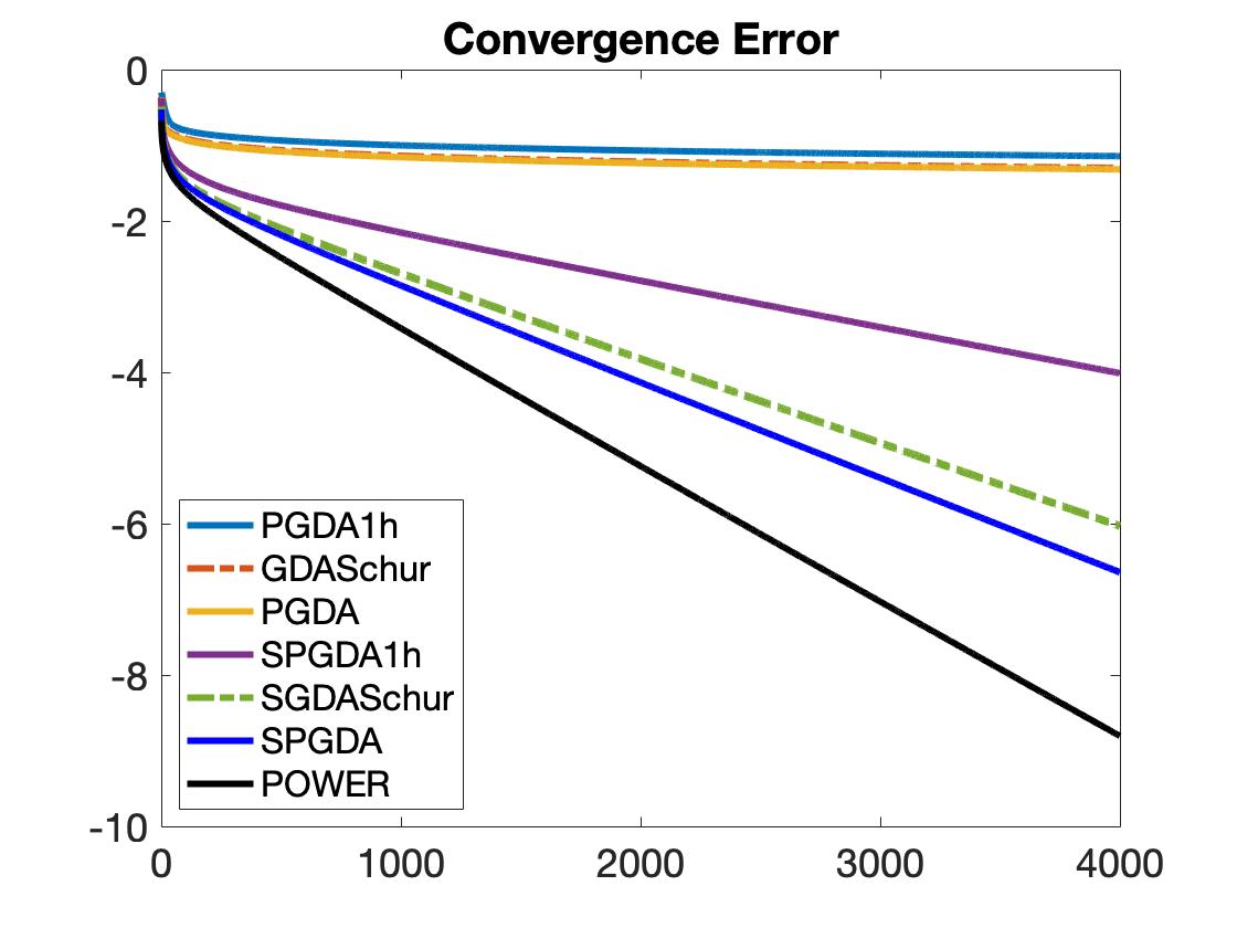
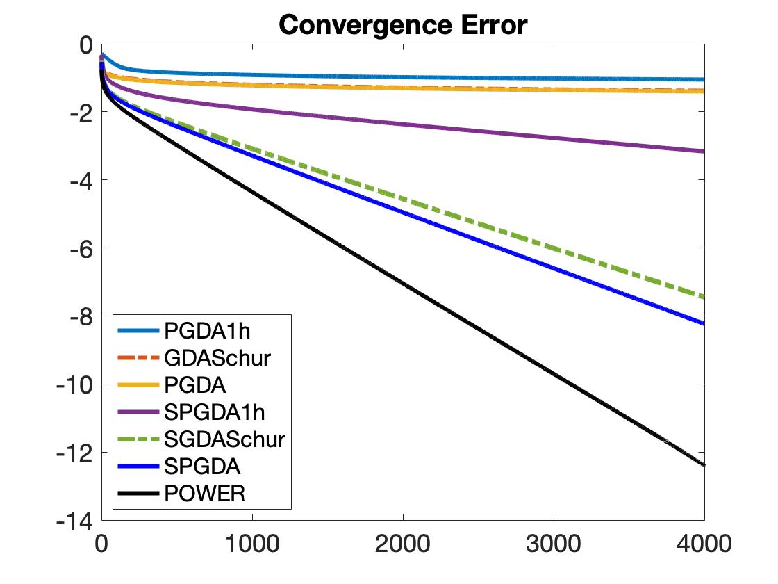
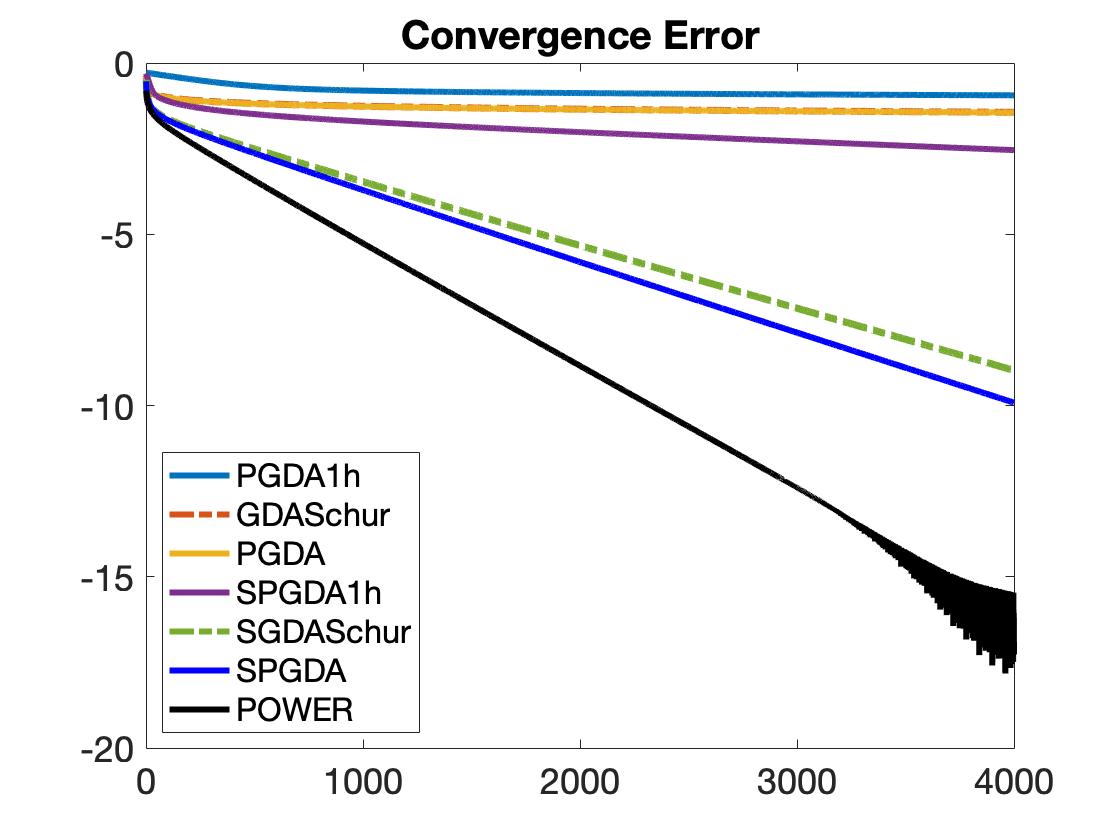
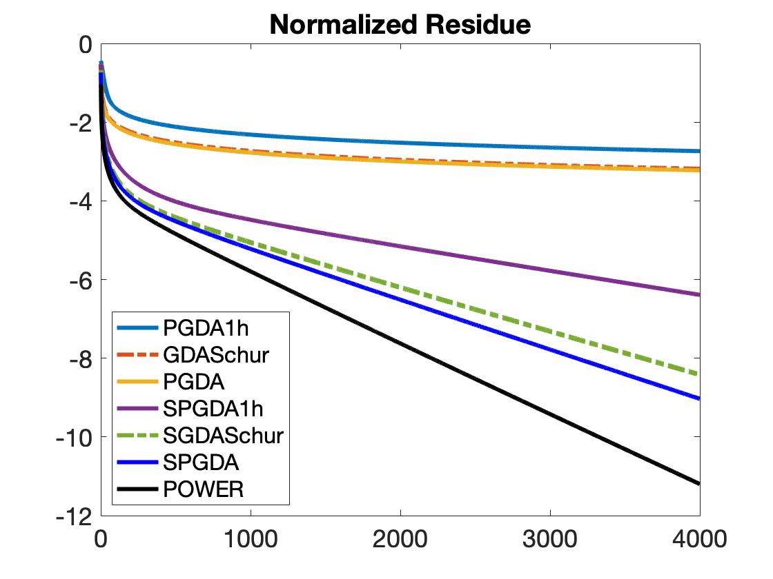
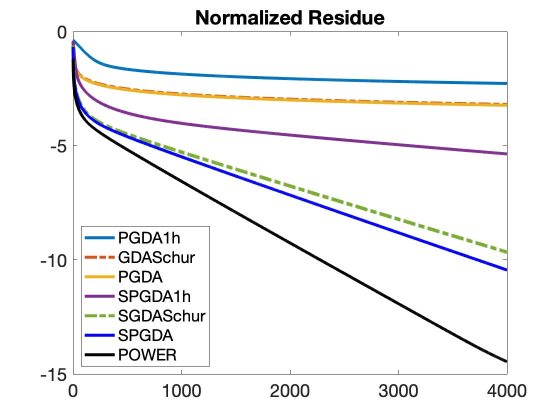
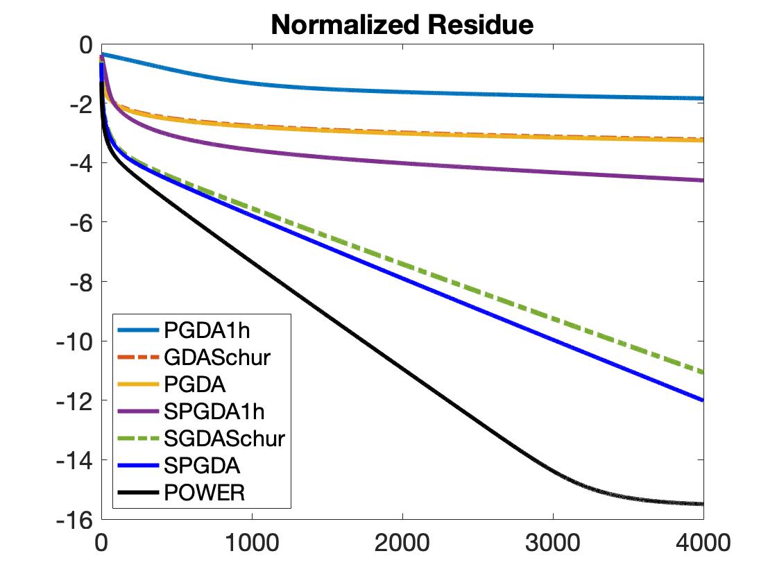
Figure 1: Plotted on the first and second rows are average over 500 trials of the convergence errors ${\rm CE}(n)$ and normalized residues ${\rm RE}(n),1\leq n\leq 4000$, in the logarithmic scale, while from left to right are lowpass spline filters ${\bf H}_{0,m}^{\rm spln}$ of orders $m=2,3,4$ on the random geometric graph ${\mathcal{G}}_{512}$.

Appendix A Proof of Theorem II.1

By nonsingularity of the matrix ${\bf Q}$, it suffices to prove

$$\|{\bf Q}({\bf x}_{n}-{\bf u})\|_{2}\leq\|{\bf Q}{\bf x}_{0}\|_{2}r^{n},\ \ n\geq 0$$ (A.1)

for some ${\bf u}$ satisfying ${\bf A}{\bf u}={\bf 0}$, where $r\in(0,1)$.

Set ${\bf B}={\bf I}-{\bf Q}^{-1}{\bf A}^{*}{\bf A}{\bf Q}^{-1}$ and let ${\bf u}_{i}$ be orthonormal eigenvectors associated with eigenvalues $\gamma_{i}$ of the Hermitian matrix ${\bf B}$ that satisfy

$${\bf B}{\bf u}_{i}=\gamma_{i}{\bf u}_{i},\ \ 1\leq i\leq N.$$ (A.2)

Following the argument in [15, Theorem II.1] and applying (II.2), we obtain that ${\bf Q}^{2}-{\bf A}^{*}{\bf A}$ is positive semidefinite. This together with nonsingularity of the matrix ${\bf Q}$ implies that

$$0\leq\gamma_{i}\leq 1,\ 1\leq i\leq N.$$ (A.3)

Write ${\bf Q}{\bf x}_{0}=\sum_{i=1}^{N}\langle{\bf Q}{\bf x}_{0},{\bf u}_{i}\rangle{\bf u}_{i}$, where $\langle\cdot,\cdot\rangle$ is the standard inner product on ${\mathbb{C}}^{N}$. By (II.3), we have that ${\bf Q}{\bf x}_{n}={\bf B}{\bf Q}{\bf x}_{n-1},\ n\geq 1$. Therefore

$${\bf Q}{\bf x}_{n}={\bf B}^{n}{\bf Q}{\bf x}_{0}=\sum_{i=1}^{N}\gamma_{i}^{n}\langle{\bf Q}{\bf x}_{0},{\bf u}_{i}\rangle{\bf u}_{i},\ n\geq 0.\vspace{-.5em}$$ (A.4)

Define ${\bf u}=\sum_{\gamma_{i}=1}\langle{\bf Q}{\bf x}_{0},{\bf u}_{i}\rangle{\bf Q}^{-1}{\bf u}_{i}$. Then by (A.3), (A.4) and the orthonormality of ${\bf u}_{i},1\leq i\leq N$, we obtain

$$\hskip-5.78172pt\|{\bf Q}({\bf x}_{n}-{\bf u})\|_{2} \hskip-5.78172pt= \hskip-5.78172pt\Big{(}\sum_{0\leq\gamma_{i}<1}|\langle{\bf Q}{\bf x}_{0},{\bf u}_{i}\rangle|^{2}\gamma_{i}^{2n}\Big{)}^{1/2}$$ (A.5)

$$\hskip-5.78172pt\leq \hskip-5.78172ptr^{n}\|{\bf Q}{\bf x}_{0}-{\bf Q}{\bf u}\|_{2}\leq r^{n}\|{\bf Q}{\bf x}_{0}\|_{2},\vspace{-.5em}$$

where $r=\max_{0\leq\gamma_{i}<1}\gamma_{i}$. This proves (A.1) and the desired exponential convergence of the sequence ${\bf x}_{n},n\geq 0$.

Taking the limit in (II.3) and applying the convergence in (A.1) yields ${\bf Q}^{-2}{\bf A}^{*}{\bf A}{\bf u}={\bf 0}$. This proves that ${\bf A}{\bf u}={\bf 0}$ and completes the proof.

References

• [1] J. Yick, B. Mukherjee, and D. Ghosal, โ€œWireless sensor network survey,โ€ Comput. Netw., vol. 52, no. 12, pp. 2292-2330, Aug. 2008.
• [2] D. I. Shuman, S. K. Narang, P. Frossard, A. Ortega, and P. Vandergheynst, โ€œThe emerging field of signal processing on graphs: Extending high-dimensional data analysis to networks and other irregular domains,โ€ IEEE Signal Process. Mag., vol. 30, no. 3, pp. 83-98, May 2013.
• [3] A. Sandryhaila and J. M. F. Moura, โ€œBig data analysis with signal processing on graphs: Representation and processing of massive data sets with irregular structure,โ€ IEEE Signal Process. Mag., vol. 31, no. 5, pp. 80-90, Sept. 2014.
• [4] D. F. Gleich, โ€œPagerank beyond the web,โ€ SIAM Review, vol. 57, no. 3, pp. 321-363, 2015.
• [5] R. Hebner, โ€œThe power grid in 2030,โ€ IEEE Spectrum, vol. 54, no. 4, pp. 50-55, Apr. 2017.
• [6] A. Langville and C. Meyer, Googleโ€™s PageRank and Beyond: The Science of Search Engine Rankings, Princeton University Press, 2006.
• [7] A. Ortega, P. Frossard, J. Kovacevic, J. M. F. Moura, and P. Vandergheynst, โ€œGraph signal processing: Overview, challenges, and applications,โ€ Proc. IEEE, vol. 106, no. 5, pp. 808-828, May 2018.
• [8] C. Cheng, Y. Jiang, and Q. Sun, โ€œSpatially distributed sampling and reconstruction,โ€ Appl. Comput. Harmon. Anal., vol. 47, no. 1, pp. 109-148, July 2019.
• [9] E. Isufi, A. Loukas, A. Simonetto, and G. Leus, โ€œAutoregressive moving average graph filtering,โ€ IEEE Trans. Signal Process., vol. 65, no. 2, pp. 274-288, Jan. 2017.
• [10] S. Segarra, A. G. Marques, and A. Ribeiro, โ€œOptimal graph-filter design and applications to distributed linear network operators,โ€ IEEE Trans. Signal Process., vol. 65, no. 15, pp. 4117-4131, Aug. 2017.
• [11] W. Waheed and D. B. H. Tay, โ€œGraph polynomial filter for signal denoising,โ€ IET Signal Process., vol. 12, no. 3, pp. 301-309, Apr. 2018.
• [12] D. I. Shuman, P. Vandergheynst, D. Kressner, and P. Frossard, โ€œDistributed signal processing via Chebyshev polynomial approximation,โ€ IEEE Trans. Signal Inf. Process. Netw., vol. 4, no. 4, pp. 736-751, Dec. 2018.
• [13] M. Coutino, E. Isufi, and G. Leus, โ€œAdvances in distributed graph filtering,โ€ IEEE Trans. Signal Process., vol. 67, no. 9, pp. 2320-2333, May 2019.
• [14] N. Emirov, C. Cheng, J. Jiang, and Q. Sun, โ€œPolynomial graph filter of multiple shifts and distributed implementation of inverse filtering,โ€ arXiv: 2003.11152, Mar. 2020.
• [15] C. Cheng, N. Emirov, and Q. Sun, โ€œPreconditioned gradient descent algorithm for inverse filtering on spatially distributed networks,โ€ IEEE Signal Process. Lett., vol. 27, pp. 1834-1838, 2020.
• [16] X. Ma, L. Gao, and X. Yong, โ€œEigenspaces of networks reveal the over- lapping and hierarchical community structure more precisely,โ€ J. Stat. Mech. Theory Exp., vol. 2010, no. 8, pp. P08012, Aug. 2010.
• [17] R. J. Sรกnchez-Garcรญa, M. Fennelly, S. Norris, N. Wright, G. Niblo, J. Brodzki, and J. W. Bialek, โ€œHierarchical spectral clustering of power grids,โ€ IEEE Trans. Power Syst., vol. 29, no. 5, pp. 2229-2237, Sept. 2014.
• [18] D. I. Shuman, M. J. Faraji, and P Vandergheynst, โ€œA multiscale pyramid transform for graph signals,โ€ IEEE Trans. Signal Process., vol. 64, no. 8, pp. 2119-2134, Apr. 2016.
• [19] A. Gusrialdi and Z. Qu, โ€œDistributed estimation of all the eigenvalues and eigenvectors of matrices associated with strongly connected digraphs,โ€ IEEE Control Syst. Lett., vol. 1, no. 2, pp. 329-333, Oct. 2017.
• [20] D. K. Hammod, P. Vandergheynst, and R. Gribonval, โ€œWavelets on graphs via spectral graph theory,โ€ Appl. Comput. Harmon. Anal., vol. 30, no. 4, pp. 129-150, Mar. 2011.
• [21] S. K. Narang and A. Ortega, โ€œPerfect reconstruction two-channel wavelet filter banks for graph structured data,โ€ IEEE Trans. Signal Process., vol. 60, no. 6, pp. 2786-2799, June 2012.
• [22] A. Sandryhaila and J. M. F. Moura, โ€œDiscrete signal processing on graphs,โ€ IEEE Trans. Signal Process., vol. 61, no. 7, pp. 1644-1656, Apr. 2013.
• [23] A. Sandryhaila and J. M. F. Moura, โ€œDiscrete signal processing on graphs: Frequency analysis,โ€ IEEE Trans. Signal Process., vol. 62, no. 12, pp. 3042-3054, June 2014.
• [24] O. Teke and P. P. Vaidyanathan, โ€œExtending classical multirate signal processing theory to graphs Part II: M-channel filter banks,โ€ IEEE Trans. Signal Process., vol. 65, no. 2, pp. 423-437, Jan. 2017.
• [25] J. Yi and L. Chai, โ€œGraph filter design for multi-agent system consensus,โ€ in IEEE 56th Annual Conference on Decision and Control (CDC), Melbourne, VIC, 2017, pp. 1082-1087.
• [26] J. Jiang, C. Cheng, and Q. Sun, โ€œNonsubsampled graph filter banks: Theory and distributed algorithms,โ€ IEEE Trans. Signal Process., vol. 67, no. 15, pp. 3938-3953, Aug. 2019.
• [27] K. Lu, A. Ortega, D. Mukherjee, and Y. Chen, โ€œEfficient rate-distortion approximation and transform type selection using Laplacian operators,โ€ in 2018 Picture Coding Symposium (PCS), San Francisco, CA, 2018, pp. 76-80.
• [28] C. Cheng, J. Jiang, N. Emirov, and Q. Sun, โ€œIterative Chebyshev polynomial algorithm for signal denoising on graphs,โ€ in Proceeding 13th Int. Conf. on SampTA, Bordeaux, France, July 2019, pp. 1-5.
• [29] P. Nathanael, J. Paratte, D. Shuman, L. Martin, V. Kalofolias, P. Vandergheynst, and D. K. Hammond, โ€œGSPBOX: A toolbox for signal processing on graphs,โ€ arXiv:1408.5781, Aug. 2014.
• [30] M. S. Kotzagiannidis and P. L. Dragotti, โ€œSampling and reconstruction of sparse signals on circulant graphs - an introduction to graph-FRI,โ€ Appl. Comput. Harmon. Anal., vol. 47, no. 3, pp. 539-565, Nov. 2019.
• [31] S. Chen, A. Sandryhaila, J. M. F. Moura, and J. Kovacevic, โ€œSignal recovery on graphs: variation minimization,โ€ IEEE Trans. Signal Process., vol. 63, no. 17, pp. 4609-4624, Sept. 2015.
• [32] G. H. Golub and C. F. V. Loan, Matrix Computations, The Johns Hopkins University Press, 2013.