Improved Confidence Bounds for the Linear Logistic Model and Applications to Bandits

Abstract

We propose improved fixed-design confidence bounds for the linear logistic model. Our bounds significantly improve upon the state-of-the-art bound by Li et al. (2017) via recent developments of the self-concordant analysis of the logistic loss (Faury et al., 2020). Specifically, our confidence bound avoids a direct dependence on $1/\kappa$, where $\kappa$ is the minimal variance over all arms’ reward distributions. In general, $1/\kappa$ scales exponentially with the norm of the unknown linear parameter $\theta^{*}$. Instead of relying on this worst case quantity, our confidence bound for the reward of any given arm depends directly on the variance of that arm’s reward distribution. We present two applications of our novel bounds to pure exploration and regret minimization logistic bandits improving upon state-of-the-art performance guarantees. For pure exploration we also provide a lower bound highlighting a dependence on $1/\kappa$ for a family of instances.

Input: Output: initialize

1 Introduction

Multi-armed bandits algorithms offer a principled approach to solve sequential decision problems under limited feedback thompson33onthelikelihood. In bandit problems, at each time step, an agent chooses an arm to pull from an available pool of arms and and receives an associated reward. Under this setting, two major objectives arise: pure exploration (aka best-arm identification) where the goal is to identify the arm with the highest average reward; and regret minimization where the goal is to maximize the total rewards gained. Bandit algorithms are widely deployed in industry, with applications spanning news recommendation (li10acontextual), ads (SawantHVAE18), online retail (Teo2016airstream), and drug discovery (kazerouni2019best). In such applications, the agent often has access to a feature vector for each arm. A common assumption is that the reward is a noisy linear measurement of the underlying feature vector of the arm being pulled. In other words, the binary reward received from a pull of the arm $x\in\mathbb{R}^{d}$ is $y_{t}=x^{\top}\theta^{\ast}+\epsilon$, $\theta^{\ast}$ is a latent parameter vector, and $\epsilon$ is subGaussian noise. In this case, there are several algorithms that are near-optimal and/or practical for pure exploration (xu2018fully; fiez2019sequential) and for regret minimization (auer2002using; chu11contextual; dani08stochastic; russo14learning).

Unfortunately, in abundant real-world use-cases the linear reward model is not realistic and instead rewards are binary. For example, the prevalent form of data arising from user interactions is binary click/no-click feedback in the web and e-commerce domains. Another example is the problem of learning the best candidate from binary pairwise comparisons, used in matching recommender systems (biswas2019seeker). In this setting, the agent has access to a set of items (e.g., shoes), and repeatedly chooses a pair of items to present to the user to choose from. The goal of the agent is to infer the user’s favorite shoe.In this paper, we use the linear logistic model for binary feedback. In other words, the binary reward received from a pull of the arm $x\in\mathbb{R}^{d}$ is $y_{t}\sim\mathsf{Bernoulli}(\mu(x^{\top}\theta^{\ast}))$, where $\mu(z)\mathrel{\mathop{\mathchar 58\relax}}=(1+e^{-z})^{-1}$ is the logistic link function.

Existing effective bandit algorithms in the linear feedback setting attempt to estimate $\theta^{\ast}$ to drive sampling. To do so, they require tight confidence intervals on the estimated mean reward $x^{\top}\theta^{*}$ of arm $x$. To adapt these algorithms to the logistic model, we require confidence intervals that account for the non-linearity introduced by the link function $\mu$. However, there is a lack of tight confidence intervals in this setting. Our work builds on previous attempts in this area to a) provide tight confidence intervals, b) adapt existing linear bandit algorithms to the logistic setting. We now detail our contributions:

The first variance-dependent fixed design confidence interval for the linear logistic model. We first consider the fixed design setting. Assume we have access to data $(x_{s},y_{s})_{s=1}^{t}\subset\mathbb{R}^{d}\times\{0,1\}$ where the reward $y_{s}$ is generated according to the logistic model. In addition we assume $y_{s}$ is conditionally independent from $\{x_{i}\}_{i=1}^{t}\setminus\{x_{s}\}$ given $x_{s}$. Let $\hat{\theta}_{t}$ be the maximum likelihood estimator (MLE) of $\theta^{*}$. We propose the first fixed design concentration inequalities such that the width: $i)$ scales with the actual variance instead of the worst-case variance $\kappa^{-1}$ that scales exponentially with $\|\theta^{*}\|$, and $ii)$ is independent of $d$. Our bound takes the form of

$$\operatorname{\mathbb{P}}\mathinner{\left(|x^{\top}(\hat{\theta}_{t}-\theta^{*})|\leq O(\|x\|_{H_{t}^{-1}(\theta^{\ast})}\sqrt{\log(t/{\delta})})\right)}\geq 1-{\delta},$$

where $H_{t}(\theta^{\ast})$ is the Fisher information matrix at $\theta^{\ast}$ matching the asymptotic bound for the MLE. By contrast, the bounds by li2017provably take a significantly looser form of $O(\kappa^{-1}\|x\|_{V_{t}^{-1}}\sqrt{\log(1/{\delta})})$ where $V_{t}$ satisfies $\kappa V_{t}\preceq H_{t}(\theta^{*})$. Our improvements in fixed design confidence bounds parallel that of faury2020improved for adaptive sampling but reduce a $\sqrt{d}$ factor required by adaptive bounds. Our confidence bound is a fundamental result in statistical learning. It tightly quantifies the amount of information learned from the training set $\{x_{s},y_{s}\}_{s=1}^{t}$ that transfers to a test point $x$, in a data-dependent non-asymptotic manner and without distributional assumptions on $\{x_{s}\}_{s=1}^{t}$. We present the full theorem and provide detailed comparisons in Section 2.

Improved pure exploration algorithms. In Section 3 we propose a new algorithm called RAGE-GLM for pure exploration in transductive linear logistic bandits, which is a novel extension of RAGE by fiez2019sequential. RAGE-GLM significantly improves both theoretical and empirical performance over the state-of-the-art algorithm by kazerouni2019best, reducing the sample complexity by a multiplicative factor of $\kappa^{-1}$. We perform empirical evaluations on a pairwise comparison problem.

Novel fundamental limits for pure exploration. While the sample complexity of RAGE-GLM does not have $\kappa^{-1}$ in the leading term of $\log(1/{\delta})$ where ${\delta}$ is the target failure rate, it has an additive dependence on $\kappa^{-1}$. In Section 4, we show that such an additive dependence is necessary via a novel moderate confidence lower bound that captures the non-asymptotic complexity of learning and is independent of transportation inequality techniques (kaufmann2016complexity). Our results also imply that there are settings where $O(e^{d})$ samples are necessary even when gaps are large, a phenomena that does not exist for linear rewards.

Improved $K$-armed contextual bandits. We employ our confidence bounds to develop improved algorithms for contextual logistic bandits. The proposed algorithm SupLogistic makes nontrivial extensions over the state-of-the-art algorithm SupCB-GLM by li2017provably. The main challenge is to $i)$ handle the confidence width that depends on the unknown $\theta^{*}$, and $ii)$ design a novel sample bucket scheme to fix an issue of SupCB-GLM that invalidates its regret bound. We show that SupCB-GLM enjoys a regret bound of $\tilde{O}(\sqrt{dT\log(K)})$ (ignoring $o(\sqrt{T})$ terms), which is a significant improvement over SupCB-GLM that has an extra $\kappa^{-1}$ factor, along with improvements in the lower-order terms. Such an improvement parallels that of faury2020improved over UCB-GLM of li2017provably where they achieve a regret bound $\tilde{O}(d\sqrt{T})$ that shaves of the factor $\kappa^{-1}$ from UCB-GLM. We discuss our improved bounds and provide more detailed comparisons in Section 5.

2 Improved Confidence Intervals for the Linear Logistic MLE

In this section we consider the fixed design setting. We assume that we have a fixed $\theta^{\ast}\in\mathbb{R}^{d}$, a set of measurements $\{(x_{s},y_{s})\}_{s=1}^{t}\subset\mathbb{R}^{d}\times\mathbb{R}$ where each $y_{s}\in\{0,1\}$, and

$$P(y_{s}=1)=\mu(x_{s}^{\top}\theta^{*})=\frac{1}{1+e^{-x^{\top}\theta^{\ast}}}.$$

Let $\eta_{s}=y_{s}-\mu(x_{s}^{\top}\theta^{*})$. Denote by $\dot{\mu}(z)$ the first order derivative of $\mu(z)$. Define $\kappa=\min_{x\mathrel{\mathop{\mathchar 58\relax}}~{}\mathinner{\!\left\lVert x\right\rVert}\leq 1}\dot{\mu}(x^{\top}\theta^{*})$.

The maximum likelihood estimate is given by:

$$\hat{\theta}\!=\!\operatorname*{arg~{}max}_{\theta\in\mathbb{R}^{d}}\sum_{s=1}^{t}y_{s}\log\mu(x_{s}^{\top}\theta)\!+\!(1\!-\!y_{s})\log(1\!-\!\mu(x_{s}^{\top}\theta))$$ (1)

We also define the Fisher information matrix at $\theta$ as

$$H_{t}(\theta)=\sum_{s=1}^{t}\dot{\mu}(x_{s}^{\top}\theta)x_{s}x_{s}^{\top}~{}.$$ (2)

We now introduce our improved confidence interval for the linear logistic model under this fixed design setting.

Theorem 1.

Let ${\delta}\leq e^{-1}$. Let $\hat{\theta}_{t}$ be the solution of Eq. (1) where, for every $s\in[t]$, $y_{s}$ is conditionally independent from $\{x_{i}\}_{i=1}^{t}\setminus\{x_{s}\}$ given $x_{s}$ (i.e. the $x_{s}$’s are a fixed design). Fix $x\in{\mathbb{R}}^{d}$ with $\|x\|\leq 1$. Let $t_{\mathsf{eff}}$ be the number of distinct vectors in $\{x_{s}\}_{s=1}^{t}$. Define ${\gamma(d)}\!=\!d+\log(6(2\!+\!{t_{\mathsf{eff}}})/{\delta})$. Define the event $\mathcal{E}_{\mathsf{var}}\!=\!\{\forall x^{\prime},{\frac{1}{\sqrt{2.2}}}\,\|x^{\prime}\|_{H_{t}(\theta^{*})^{-1}}\!\leq\!\|x^{\prime}\|_{H_{t}(\hat{\theta}_{t})^{-1}}\!\leq\!\sqrt{2.2}\,\|x^{\prime}\|_{H_{t}(\theta^{*})^{-1}}\}$. If ${\xi^{2}_{t}}\mathrel{\mathop{\mathchar 58\relax}}=\max_{s\in[t]}\|x_{s}\|^{2}_{H_{t}(\theta^{*})^{-1}}\leq{\frac{1}{\gamma(d)}}$, then

$$\operatorname{\mathbb{P}}\mathinner{\left(\!|x^{\top}\!(\hat{\theta}_{t}\!-\!\theta^{*})|\!\leq\!3.5\|x\|_{\!H_{t}(\theta^{*}\!)^{-\!1}}\textstyle\!\sqrt{\log{\frac{2(2+{t_{\mathsf{eff}}})}{{\delta}}}},\mathcal{E}_{\mathsf{var}}\!\right)}\!\geq\!1\!-\!{\delta}.$$

Remark 1.

One can see that Theorem 1 implies empirical concentration inequality $|x^{\top}\!(\hat{\theta}_{t}\!-\!\theta^{*})|\!\leq\!5.2\|x\|_{\!H_{t}({\hat{\theta}}_{t}\!)^{-\!1}}\sqrt{\log{\frac{2(2+{t_{\mathsf{eff}}})}{{\delta}}}}$. This seemingly useful bound is in fact never used in our bandit analysis for technical reasons. Specifically, bandits select arms adaptively, which breaks the fixed design assumption of Theorem 1, so care is needed for algorithmic design.

Asymptotically, under some conditions we expect for any $x\in\mathbb{R}^{d}$, $x^{\top}(\hat{\theta}-\theta)\rightarrow N(0,\|x\|^{2}_{H(\theta^{\ast})^{-1}})$ (lehmann2006theory). Our bound matches this asymptotic rate up to constant factors.

Comparison to previous work. Our theorem is a significant improvement upon li2017provably. Their bound depends on ${\frac{1}{\kappa}}\|x\|_{V_{t}^{-1}}$, with $V_{t}\mathrel{\mathop{\mathchar 58\relax}}=\sum_{s=1}^{t}x_{s}x_{s}^{\top}$. In general since $\kappa V_{t}\preceq H_{t}(\theta^{*})$, our bound is tighter and depends on the asymptotic variance. For the bound in (li2017provably) to hold, they require that $\lambda_{\min}(V_{t})\geq\Omega(d^{2}\kappa^{-4})$, which we call the burn-in condition. Recall that $\kappa^{-1}=\Theta(\exp(\|\theta^{*}\|))$ can be large even for moderate $\theta^{*}$. In contrast, our bound’s burn-in condition does not directly depend on $\kappa^{-1}$, and more importantly, it is possible to satisfy it without $\kappa^{-1}$ samples in certain cases. For example, we show in our supplementary a case where a sample size of $\mathsf{polynomial}(\|\theta^{*}\|)\ll\exp(\|\theta^{*}\|)$ can satisfy the burn-in condition. For the sake of comparison, we can use the bound $\xi_{t}^{2}\leq\kappa^{-1}\lambda_{\min}(V_{t})$ to derive an inferior burn-in condition of $\lambda_{\min}(V_{t})\geq\Omega(d\kappa^{-1})$. This is still a strict improvement over li2017provably, saving a factor of $d$ and a cubic factor in $\kappa^{-1}$ as well as shaving off their large constant factor of 512.

We now compare our bound with that of faury2020improved. The proof of Lemma 3 of faury2020improved, under the assumption that $\|\theta^{*}\|\leq S_{*}$ and with a proper choice of regularization constant, implies the following confidence bound: w.p. at least $1-{\delta}$, $\forall t\geq 1,\forall x\in{\mathbb{R}}^{d}\mathrel{\mathop{\mathchar 58\relax}}\|x\|\leq 1,$

$$x^{\top}(\hat{\theta}_{t}-\theta^{*})\leq\Theta\left(\|x\|_{H_{t}(\theta^{*})^{-1}}S_{*}^{3/2}\sqrt{(d+\log(t/{\delta})})\right)~{}.$$

While their bound also does not directly depend on $\kappa$ it is an anytime confidence bound that holds for all $x\in\mathbb{R}^{d}$ simultaneously, and in addition allows for an adaptively chosen sequence of measurements. As a result, their bound suffers an additional factor of $\sqrt{d}$. Furthermore, their bound introduces a factor $S_{*}^{3/2}$ and requires the knowledge of both $S_{*}$ and $\kappa$. In contrast, our bound does not directly depend on the confidence width nor require the knowledge of $S_{*}$ or $\kappa$ though these quantities may be needed to satisfy the burn-in condition.

Tightness of our bound. Empirically, we have observed that $\xi_{t}^{2}\leq O(1)$ is necessary to control the confidence width as a function of $\|x\|_{H_{t}(\theta^{*})^{-1}}$, but have not found a case where $\xi_{t}^{2}$ must be smaller than $O(1/d)$; studying the optimal burn-in condition is left as future work. We believe one can improve $\log({t_{\mathsf{eff}}})$ to the metric entropy of the measurements $\{x_{s}\}_{s=1}^{t}$. Note that it is possible to remove the burn-in condition if we derive a regularized MLE version of Theorem 1, but this comes with an extra factor of $\sqrt{d}$ in the confidence width, which is not better than the confidence bound of faury2020improved.

Proof Sketch of Theorem 1.

The novelty of our argument is to exploit the variance term without introducing $\kappa$ explicitly in the confidence width. We follow the main decomposition of li2017provably but deviate from their proof by: $i)$ employing Bernstein’s inequality rather than Hoeffding’s to obtain $H_{t}(\theta^{*})$ in the bound (as opposed to $\kappa^{-1}V_{t}$); and $ii)$ deriving a novel implicit inequality on $\max_{s\in[t]}|x_{s}^{\top}({\hat{\theta}}_{t}-\theta^{*})|$. The latter leads to the significant improvements in both $d$ and $\kappa^{-1}$ in the condition on $\xi_{t}$.

Let $\alpha_{s}(\hat{\theta}_{t},\theta^{*})\mathrel{\mathop{\mathchar 58\relax}}=\frac{\mu(x_{s}^{\top}\hat{\theta}_{t})-\mu(x_{s}^{\top}\theta^{*})}{x_{s}^{\top}(\hat{\theta}_{t}-\theta^{*})}$, $z\mathrel{\mathop{\mathchar 58\relax}}=\sum_{s}^{t}\eta_{s}x_{s}$, and $G\mathrel{\mathop{\mathchar 58\relax}}=\sum_{s}^{t}\alpha_{s}(\hat{\theta}_{t},\theta^{*})x_{s}x_{s}^{\top}$. By the optimality condition of $\hat{\theta}_{t}$, we have:

$$\begin{split}z&=G(\hat{\theta}_{t}-\theta^{*}).\end{split}$$ (3)

We use the shorthand $H\mathrel{\mathop{\mathchar 58\relax}}=H_{t}(\theta^{*})$ and define $E\mathrel{\mathop{\mathchar 58\relax}}=G-H$. The main decomposition is

$$|x^{\top}(\hat{\theta}_{t}-\theta^{*})| \!=\!|x^{\top}(H+E)^{-1}z|$$ (4)

$$\!\leq\!|x^{\top}H^{-1}z|+|x^{\top}H^{-1}E(H+E)^{-1}z|~{}.$$

We bound $x^{\top}H^{-1}z$ by $O(\|x\|_{H^{-1}}\sqrt{\log(1/{\delta})})$ which uses Bernstein’s inequality and the assumption on $\xi^{2}_{t}$. We control the second term by:

$$|x^{\top}H^{-1}E(H+E)^{-1}z|$$

$$\leq\|x\|_{H^{-1}}\|H^{-1/2}EH^{-1/2}\|\|G^{-1}z\|_{H}$$ (5)

$$\stackrel{{\scriptstyle(a)}}{{\leq}}\|x\|_{H^{-1}}\|H^{-1/2}EH^{-1/2}\|(1+D)\|z\|_{H^{-1}}$$

$$\stackrel{{\scriptstyle(b)}}{{\leq}}\|x\|_{H^{-1}}\|H^{-1/2}EH^{-1/2}\|(1+D)\cdot O(\sqrt{d+\log(1/{\delta})})$$

$$\stackrel{{\scriptstyle(c)}}{{\leq}}\|x\|_{H^{-1}}D\cdot O(\sqrt{d+\log(1/{\delta})}),$$

where $(a)$ is by introducing $D\mathrel{\mathop{\mathchar 58\relax}}=\max_{s\in[t]}|x_{s}^{\top}({\hat{\theta}}-\theta^{*})|$ and using the self-concordance property of the logistic loss (faury2020improved), $(b)$ is Bernstein’s inequality with a covering argument along with the assumption on $\xi_{t}$, and $(c)$ is by a novel result employing self-concordance and the assumption to show that $E$ can be bounded by $D\cdot H$. Our key observation is to apply Eq. (4) for every distinct vector $x$ in $\{x_{s}\}_{s\in[t]}$ and employ $\|x\|_{H^{-1}}\leq\xi_{t}$ to see:

$$D =\max_{s\in[t]}|x_{s}^{\top}({\hat{\theta}}-\theta^{*})|$$

$$\leq O(\xi_{t}\sqrt{\log(1/{\delta})})+\xi_{t}D\cdot O(\sqrt{d+\log(1/{\delta})})~{}.$$

The assumption on $\xi_{t}$ implies $\xi_{t}O(\sqrt{d+\log(1/{\delta})})<1$. We solve for $D$ to obtain the implicit equation

$$D=O(\xi_{t}\sqrt{1/{\delta}})~{}.$$

Plugging this back into Eq. (2) gives $\|x^{\top}({\hat{\theta}}-\theta^{*})\|\leq O(\|x\|_{H^{-1}}\sqrt{\log(1/{\delta})})$, which holds with probability at least $1-\Theta({t_{\mathsf{eff}}}\delta)$, as we use the concentration inequality $\Theta({t_{\mathsf{eff}}})$ times. To turn this into a statement that holds w.p. at least $1-{\delta}$, we substitute ${\delta}$ with $\Theta({\delta}/{t_{\mathsf{eff}}})$, concluding the proof. See appendix for the statement on $\mathcal{E}_{\mathsf{var}}$. ∎

3 Transductive Pure Exploration

We now consider the linear logistic pure exploration problem. Specifically, the learner is given a confidence level ${\delta}\in(0,1)$ and has access to finite arm subsets $\mathcal{X},\mathcal{Z}\subset\mathbb{R}^{d}$ but not the problem parameter $\theta^{*}\in{\mathbb{R}}^{d}$. The goal is to discover $z^{\ast}=\arg\max_{z\in\mathcal{Z}}z^{\top}\theta^{\ast}$ with probability at least $1-\delta$ using as few measurements from $\mathcal{X}$ as possible. This is a generalization of the standard linear pure exploration (soare2014best) and is referred to as the transductive setting (fiez2019sequential). In each time step $t$, the learner chooses an arm $x_{t}$, which is measurable with respect to the history $\mathcal{F}_{t-1}=\{(x_{s},y_{s})_{s<t}\}$, and observes a reward $y_{t}\in\{0,1\}$. It stops at a random stopping time $\tau$ and recommends $\hat{z}\in\mathcal{Z}$, where $\tau$ and $\hat{z}$ are both measurable w.r.t. the history $\mathcal{F}_{\tau}$. We assume that $\mathbb{P}(y_{t}=1|x_{t},\mathcal{F}_{t-1})=\mu(x_{t}^{\top}\theta^{\ast})$. Let $\mathbb{P}_{\theta},\mathbb{E}_{\theta}$ denote the probability and expectation induced by the actions and rewards when the true parameter is $\theta$. Formally, we define a $\delta$-PAC algorithm as follows: An algorithm for the logistic-transductive-bandit problem is $\delta$-PAC for $(\mathcal{X},\mathcal{Z})$ if $\mathbb{P}_{\theta}(z_{\tau}\neq z^{\ast})\leq\delta\ ,\forall\theta\in\mathbb{R}^{d}$.

Example: Pairwise Judgements. As a concrete and natural example, consider an e-commerce application where the goal is to recommend an item from a set of items based on relative judgements by the user. For example, the user may be repeatedly shown two items to compare, and must choose one. In each round, the system chooses two items $z,z^{\prime}\in\mathcal{Z}$, and observes the binary user preference of item $z$ or item $z^{\prime}$. A natural model is to give each item $z\in\mathcal{Z}$ a score $z^{\top}\theta^{\ast}$, with the goal of finding $z^{\ast}=\max_{z\in\mathcal{Z}}z^{\top}\theta^{\ast}$. The probability the user prefers item $z$ over $z^{\prime}$ is modeled by $\mathbb{P}(z>z^{\prime})=\mu((z-z^{\prime})^{\top}\theta^{\ast})$. Hence the set of measurement vectors is naturally $\mathcal{X}=\{z-z^{\prime}\mathrel{\mathop{\mathchar 58\relax}}z,z^{\prime}\in\mathcal{Z}\}$. Note that our setting is a natural generalization of the dueling bandit setting (Yue2012Dueling). As far as we are aware, this is the first work to propose the dueling bandit problem as a natural extension of the transductive linear bandit setting under a logistic noise model.

Related Work. soare2014best first proposed the problem of pure exploration in linear bandits with Gaussian noise when $\mathcal{X}=\mathcal{Z}$. fiez2019sequential introduced the general transductive setting, provided the RAGE elimination based method which is the main inspiration for our algorithm. RAGE achieves the lower bound up to logarithmic factors with excellent empirical performance. Other works include degenne2020gamification; karnin2013almost, which achieve the lower bound asymptotically. Finally we mention katz2020empirical, which follows a similar approach to fiez2019sequential but uses empirical process theory to replace the union bound over the number of arms with a Gaussian width.

Despite its importance in abundant real-life settings, pure-exploration for logisitic bandits has received little attention. The only work we are aware of is kazerouni2019best which defines the problem and provides an algorithm motivated by xu2018fully. However, their theoretical and empirical performance are both far behind our proposed algorithm RAGE-GLM as we elaborate more below.

Notation. Define $\kappa_{0}=\min_{x\in\mathcal{X}}\dot{\mu}(x^{\top}\theta^{\ast})$, the smallest derivative of the link function among elements in $\mathcal{X}$ (differing slightly from the previous section). Let $\Delta_{\mathcal{X}}=\{\lambda\in\mathbb{R}^{|\mathcal{X}|},\lambda\geq 0,\sum_{x\in\mathcal{X}}\lambda_{x}=1\}$ be the probability simplex over $\mathcal{X}$. Given a design $\lambda\in\Delta_{\mathcal{X}}$, define:

$$H(\lambda,\theta)\mathrel{\mathop{\mathchar 58\relax}}=\sum_{x\in\mathcal{X}}\lambda_{x}\dot{\mu}(x^{\top}\theta)xx^{\top},\;A(\lambda)\mathrel{\mathop{\mathchar 58\relax}}=\sum_{x\in\mathcal{X}}\lambda_{x}xx^{\top}.$$

3.1 Algorithm

Algorithm 1 RAGE-GLM

$\epsilon$, $\delta$, $\mathcal{X}$, $\mathcal{Z}$, $\kappa_{0}$, effective rounding procedure $\text{{round}}(n,\epsilon,\lambda)$$k=1,\mathcal{Z}_{1}=\mathcal{Z},r(\epsilon)=d^{2}/\epsilon$$\hat{\theta}_{0}\leftarrow$BurnIn($\mathcal{X},\kappa_{0}$) Burn-in phase $|\mathcal{Z}_{k}|>1$Elimination phase $\delta_{k}=\delta/(2k^{2}\max\{|\mathcal{Z}|,|\mathcal{X}|\}(2+|\mathcal{X}|))$$f(\lambda)\mathrel{\mathop{\mathchar 58\relax}}=\max\Big{[}\gamma(d)\max_{x\in\mathcal{X}}\|x\|_{H(\lambda,\hat{\theta}_{k-1})^{-1}}^{2}$, $2^{2k}\cdot(3.5)^{2}\max_{z,z^{\prime}\in\mathcal{Z}_{k}}\|z-z^{\prime}\|_{H(\lambda,\hat{\theta}_{k-1})^{-1}}^{2}\Big{]}$$\lambda_{k}=\operatorname*{arg~{}min}_{\lambda\in\Delta_{\mathcal{X}}}f(\lambda)$$n_{k}=\max\{3(1+\epsilon)f(\lambda_{k})\log(1/\delta_{k}),r(\epsilon)\}$$x_{1},\cdots,x_{n_{k}}\leftarrow\text{{round}}(n,\epsilon,\lambda)$Observe rewards $y_{1},\cdots,y_{n_{k}}\in\{0,1\}$. Compute the MLE $\hat{\theta}_{k}$with $\{(x_{i},y_{i})\}_{i=1}^{n_{k}}$. Eq () $\hat{z}_{k}=\arg\max_{z\in\mathcal{Z}_{k}}\hat{\theta}_{k}^{\top}z$$\mathcal{Z}_{k+1}\leftarrow\mathcal{Z}_{k}\setminus\left\{z\in\mathcal{Z}_{k}\mathrel{\mathop{\mathchar 58\relax}}\hat{\theta}_{k}^{\top}(\hat{z}_{k}-z)\geq 2^{-k}\right\}$$k\leftarrow k+1$$\hat{z}_{k}$

Our RAGE-GLM algorithm (Alg. 1) proceeds in rounds. In each round $k$, it maintains a set of active arms $\mathcal{Z}_{k}$. It computes an experimental design that is dependent on $\hat{\theta}_{k-1}$, the estimate of $\theta^{\ast}$ from the previous round, and uses this experimental design to draw $n_{k}$ samples. Then, the algorithm eliminates any arms verified to be sub-optimal using $\hat{\theta}_{k}$. We now go into the algorithmic details.

Rounding. In the $k$-th round, we have $H_{k}(\theta)\mathrel{\mathop{\mathchar 58\relax}}=\sum_{s=1}^{n_{k}}\dot{\mu}(x_{s}^{\top}\theta)x_{s}x_{s}^{\top}$. The algorithm utilizes an efficient rounding procedure to ensure that $H_{k}(\hat{\theta}_{k-1})$ is within a constant factor of $n_{k}\cdot H(\lambda_{k},\hat{\theta}_{k-1})$. Given distribution $\lambda_{k}$, tolerance $\epsilon$, and a number of samples $n_{k}\geq r(\epsilon)$, the procedure $\text{{round}}(n_{k},\epsilon,\lambda)$ returns an allocation $\{x_{s}\}_{s=1}^{n_{k}}$ such that for any $\theta\in\mathbb{R}^{d}$, $H_{k}(\theta)\geq\frac{n_{k}}{1+\epsilon}H(\lambda,\theta)$. Efficient rounding procedures with $r(\epsilon)=d^{2}/\epsilon$ are described in (fiez2019sequential); see the supplementary for more details.

Algorithm 2 BurnIn

$\mathcal{X},\kappa_{0}$$\lambda_{0}=\arg\min_{\lambda\in\Delta_{\mathcal{X}}}\max_{x\in\mathcal{X}}\|x\|_{A(\lambda)^{-1}}^{2}$$n_{0}=3(1+\epsilon)\kappa_{0}^{-1}d\gamma(d)\log(2|\mathcal{X}|(2+|\mathcal{X}|)/\delta)$$x_{1},\cdots,x_{n_{0}}\leftarrow\text{{round}}(n_{0},\lambda_{0},\epsilon)$Observe associated rewards $y_{1},\cdots,y_{n_{0}}$. MLE $\hat{\theta}_{0}$Use Eq (1)

Burn-In Phase. The burn-in phase computes $\hat{\theta}_{0}$, an estimate of $\theta^{\ast}$ to be used in the first round. To do so, we need to guarantee that $\theta^{\ast}$ is well-estimated in all directions $\mathcal{X}$, i.e., $|x^{\top}(\hat{\theta}-\theta^{\ast})|<1,\forall x\in\mathcal{X}$. Ensuring this requires that we can employ the confidence interval in Theorem 1. Thus, burn-in Algorithm 2 must ensure that $\max_{x\in\mathcal{X}}\|x\|^{2}_{(\sum_{s=1}^{n_{0}}\dot{\mu}(x_{s}^{\top}\theta^{\ast})x_{s}x_{s}^{\top})^{-1}}\leq 1/\gamma(d)$. As we yet lack information on $\theta^{\ast}$, we take the naive approximation:

$$\sum_{s=1}^{n_{0}}\dot{\mu}({\theta^{\ast}}^{\top}x_{s})x_{s}x_{s}^{\top} \geq\frac{n_{0}}{1+\epsilon}H(\lambda,\theta)\quad\text{(from rounding)}$$

$$\geq\frac{n_{0}}{1+\epsilon}\kappa_{0}A(\lambda),$$

and instead consider the optimization problem $\min_{\lambda\in\mathcal{X}}\max_{x\in\mathcal{X}}\|x\|_{A(\lambda)^{-1}}^{2}$. This is a G-optimal experimental design, and has a value of $d$ by the Kiefer-Wolfowitz theorem (soare2014best). For the burn-in phase we assume we have access to an upper bound on $\kappa_{0}^{-1}$, which is equivalent to knowing an upper bound on $\|\theta^{*}\|$.

Experimental Design. In each round, line 1 of Algorithm 1 optimizes a convex experimental design that minimizes two objectives simultaneously. The main objective is

$$2^{2k}\min_{\lambda\in\Delta_{\mathcal{X}}}\max_{z,z^{\prime}\in\mathcal{Z}_{k}}\|z-z^{\prime}\|^{2}_{H(\lambda,\hat{\theta}_{k-1})^{-1}}.$$ (6)

which ensures the the gap $\theta^{\top}(z^{\ast}-z)$ is estimated to an error of $2^{-k}$ for each $z$. This allows us to eliminate arms whose gaps are significantly larger than $2^{-k}$ in each round, guaranteeing that $\mathcal{Z}_{k}\subset\mathcal{S}_{k}\mathrel{\mathop{\mathchar 58\relax}}=\{z\mathrel{\mathop{\mathchar 58\relax}}(z^{\ast}-z)^{\top}\theta^{\ast}\leq 2\cdot 2^{-k}\}$.

The other component of line 1 minimizes $\max_{x\in\mathcal{X}}\|x\|_{H(\lambda,\hat{\theta}_{k-1})^{-1}}^{2}$ similarly to the burn-in phase. This guarantees that we satisfy the conditions of Theorem 1. It additionally guarantees that the estimate $\hat{\theta}_{k}$ is sufficiently close to $\theta^{\ast}$ for all directions in $\mathcal{X}$. Combining this with self-concordance, $|\ddot{\mu}|\leq\dot{\mu}$, we show that $H(\lambda_{k},\theta^{\ast})$ is within a constant factor of $H(\lambda_{k},\hat{\theta}_{k})$ (see the supplementary). We stop when $|\mathcal{Z}_{k}|=1$ and return the remaining arm.

Theorem 2 (Sample Complexity).

Take $\delta<1/e$ and assume $\|z\|\leq 1/2$ for all $z\in\mathcal{Z}$. Define

$$\beta_{k}=\min_{\lambda\in\Delta_{\mathcal{X}}}\max\bigg{[}2^{2k}\max_{z,z^{\prime}\in\mathcal{S}_{k}}\|z-z^{\prime}\|_{H(\lambda,\theta^{\ast})^{-1}}^{2},$$

$$\gamma(d)\max_{x}\|x\|_{H(\lambda,\theta^{\ast})^{-1}}^{2}\bigg{]}$$

Algorithm 1 returns $z^{\ast}$ with probability greater than $1-3\delta$ in a number of samples no more than

$$O\bigg{(}\sum_{k=1}^{\lceil\log_{2}(2/\Delta_{\min})\rceil}\beta_{k}\log(\max\{|\mathcal{Z}|,|\mathcal{X}|\}k^{2}/\delta)$$

$$+d(1+\epsilon)\gamma(d)\kappa_{0}^{-1}\log(|\mathcal{X}|/\delta)+r(\epsilon)\log(\Delta_{\min}^{-1})\bigg{)}$$

where $\Delta_{\min}=\min_{z\neq z^{\ast}\in\mathcal{Z}}\langle\theta^{\ast},z^{\ast}-z\rangle$.

Interpreting the Upper Bound. Before comparing our bound with prior work, we show concrete examples that show the strength of our sample complexity bound.

Example 1. Consider a simple setting where $\mathcal{Z}=\mathcal{X}=\{e_{1},e_{2}\}\subset{\mathbb{R}}^{2}$, and $\theta^{\ast}=(r,r-\epsilon)$, for $r\geq 0$. In this case, $\kappa_{0}^{-1}=\max_{i\in\{1,2\}}\dot{\mu}(z_{i}^{\top}\theta^{\ast})^{-1}\leq e^{r}$. Thus in the burn-in phase, we take roughly $\tilde{O}(e^{r})$ samples. Now, for small $\epsilon$, the minimizer of $\min_{\lambda\in\Delta_{\mathcal{X}}}\|e_{1}-e_{2}\|_{H(\theta^{\ast})^{-1}}^{2}$ places roughly equal mass on $e_{1}$ and $e_{2}$, giving an objective value that is roughly bounded by $e^{r}$. Thus the sample complexity of Algorithm 1 is $O(\sum_{k=1}^{\log_{2}(1/\epsilon)}2^{2k}e^{r}\log(1/\delta))\approx\frac{e^{r}}{\epsilon^{2}}$.

Note this problem is equivalent to a standard best-arm identification algorithm with two Bernoulli arms (kaufmann2015complexity). Standard results in Pure Exploration show that a lower bound on this problem is given by the KL-divergence $\mathsf{KL}({\mathsf{Bernoulli}}(\mu(\theta^{\top}\!z_{1})),{\mathsf{Bernoulli}}(\mu(\theta^{\top}\!z_{2})))^{-1}\!\approx\!\frac{e^{r}}{2\epsilon^{2}}$ for sufficiently small $\epsilon$. This shows that our bound is at least no worse than the well-studied unstructured case.

Example 2. We extend the above setting and consider $\mathcal{X}=\{e_{1},e_{2},e_{1}-e_{2}\}$, $\mathcal{Z}=\{e_{1},e_{2}\}$ and the same $\theta^{\ast}$. As above, the burn-in phase requires $\kappa^{-1}\approx e^{r}$ samples. Starting from the first round, our computed experimental design will place all of its samples on the third arm. In this case, $\min_{\lambda}\|e_{1}-e_{2}\|_{H(\theta^{\ast})^{-1}}^{2}=1/\dot{\mu}(\epsilon)\leq C$, for small $\epsilon$. The main term of the sample complexity becomes

$$O\mathinner{\left(\sum_{k=1}^{\log_{2}(1/\Delta_{\min})}2^{2k}\log\frac{1}{\delta}\right)}\leq O\mathinner{\left(\frac{1}{\epsilon^{2}}\log\frac{1}{\delta}\right)}~{}.$$

Hence ignoring burn-in or the additional samples we take in each round to guarantee the confidence interval, the total sample complexity would be $\tilde{O}(\frac{1}{\epsilon^{2}})$. This is exponentially smaller than in Example 1 and demonstrates the power of an informative arm in reducing the sample complexity.

On the other hand, the burn-in phase, common to all logistic bandit algorithms based on the MLE, may potentially take a number of samples exponential in $r$. This example demonstrates the need for further work on understanding the precise dependence of $\kappa$ in pure exploration. In Section 4, we take a first step towards this by showing $\kappa^{-1}$ burn-in is unavoidable in some cases.

Comparison to past work. As $\beta_{k}$ grows exponentially each round, the first element in the maximum for $\beta_{k}$ dominates our sample complexity. Focusing on this term while ignoring logarithmic terms and the burn-in samples, the sample complexity in Theorem 2 scales as

$$\rho*\mathrel{\mathop{\mathchar 58\relax}}=\sum_{k=1}^{\log_{2}(2/\Delta_{\min})}2^{2k}\min_{\lambda\in\Delta_{\mathcal{X}}}\max_{z,z^{\prime}\in\mathcal{S}_{k}}\|z-z^{\prime}\|_{H(\theta^{\ast})}^{2}~{}.$$

Importantly, this depends on $H(\theta^{\ast})$ instead of a loose bound based on $\kappa^{-1}$. In the supplementary we show

$$\rho*\leq\log\left(\frac{2}{\Delta_{\min}}\right)\min_{\lambda\in\Delta_{\mathcal{X}}}\max_{z\in\mathcal{Z}\setminus z^{\ast}}\frac{\|z^{\ast}-z\|_{H(\lambda,\theta^{\ast})^{-1}}^{2}}{\langle\theta^{\ast},z^{\ast}-z\rangle^{2}}.$$

This is reminiscent of a similar quantity that is within a $\log(\cdot)$ factor of being optimal for pure exploration linear bandits (fiez2019sequential). We provide a close connection between our upper bound and information theoretic lower bounds in the supplementary, although they do not match exactly. We also prove a novel lower bound in moderate confidence regimes, which we elaborate more in Section 4.

We now compare to the result of kazerouni2019best. Using a variant of the UGapE algorithm for linear bandits (xu2018fully), they demonstrate a sample complexity $\tilde{O}(\frac{d|\mathcal{X}|}{\kappa^{2}\Delta^{2}_{\min}})$ in the setting where $\mathcal{X}=\mathcal{Z}$. This sample complexity, unlike ours, scales linearly with the number of arms, and only captures a dependency on the smallest gap. We note that one can improve on their sample complexity by using a naive passive algorithm that uses a fixed G-optimal design, along with the trivial bound $H(\lambda,\theta^{\ast})\geq\kappa_{0}A(\lambda)$, resulting in $\tilde{O}(d/(\kappa_{0}\Delta_{\min}^{2}))$ (soare2014best). In contrast, the bound of Theorem 2 only depends on the number of arms logarithmically, captures a local dependence on $\theta^{\ast}$, and has a better gap dependence.

Extra samples. Algorithm 1 potentially samples in each round to ensure the confidence interval is valid (i.e., the first argument of the $\max$ in line 1). In our supplementary, we propose RAGE-GLM-2 that removes these samples needed in each round (but not the burn-in samples) by employing the confidence interval of faury2020improved. This algorithm has a better asymptotic behavior as $\delta\rightarrow 0$, but could perform worse with large $d$ or $S_{\ast}$ due to an additional factor of $\sqrt{d}$ and a factor of $S_{\ast}^{3}$.

3.2 Experiments

This section evaluates the empirical performance of RAGE-GLM, alongside two additional algorithms:

• RAGE-GLM-R: This is a heuristic version of RAGE-GLM that makes two changes. First, it does not do a burn-in in each round and samples from $\lambda_{k}=\min_{z,z^{\prime}}\|z-z^{\prime}\|_{H(\lambda,\hat{\theta}_{k-1})^{-1}}^{2}$ directly. Second, to compute the estimate $\hat{\theta}_{k}$, it uses all samples up to round $k$.

• Passive Baseline: This baseline runs the burn-in procedure and then computes the static design $\lambda=\min_{z,z^{\prime}\in\mathcal{Z}}\|z-z^{\prime}\|_{H(\lambda,\hat{\theta}_{0})^{-1}}^{2}$. It then proceeds in rounds, drawing $2^{k}$ samples in round $k$, terminating when we are able to verify that each arm is sub-optimal using the fixed design confidence interval (see Appendix for details). As in the heuristic, we recycle samples over rounds.

Remark. We also implemented the algorithm of (kazerouni2019best). However a) the algorithm was extremely slow to run since an MLE and a convex optimization had to be run each round, b) the confidence bounds do not exploit the true variance. As a result, the algorithm did not terminate on any of our examples.

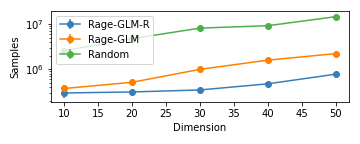
Figure 1: Standard Baseline Example

	open	pointy	sporty	comfort
$|\mathcal{Z}|$	3327	2932	3219	3374
RAGE-GLM-R	9.17e+07	2.38e+05	2.29e+05	3.34e+06
RAGE-GLM	9.17e+07	2.38e+05	2.29e+05	4.55e+06
Passive	2.69e+08	2.38e+05	2.29e+05	8.54e+06

Table 1: Zappos pairwise comparison data, bold indicates a win.

Our first experiment (Fig. 1) is a common baseline in the linear bandits literature. We consider $d+1$ arms in $d$ dimensions with arm $i\in[1,n]$ being the $i$-th basis vector, and arm $i+1$ as $\cos(.1)e_{1}+\sin(.1)e_{2}$. We use $d\in\{10,20,30,40,50\}$ and 10 repetitions for each value of $d$. In all instances, all algorithms found the best arm correctly. RAGE-GLM was competitive against the heuristic RAGE-GLM-R and took roughly a factor of 10 less samples compared to Random.

Our next experiment is based on the Zappos pairwise comparison dataset (finegrained; semjitter). This dataset consists of pairwise comparisons on 50k images of shoes and 960 dimensional vision-based feature vectors for each shoe. Given a pair of shoes, participants were asked to compare them on the the attributes of “open”, “pointy”, “sporty” and “comfort” obtaining several thousand queries. For each one of these categories, we fit a logistic model to the set of pairwise comparisons after PCA-ing the features down to 25 dimensions (for computational tractability) and used the underlying weights as $\theta^{\ast}$. We then set $\mathcal{Z}$ to be the set of shoes that were considered in that category and $\mathcal{X}$ to be 5000 random pairs. Table 1 shows the result. For the “open” and “comfort” category, RAGE-GLM took about a factor of 3 less samples compared to Random. The large sample complexity for “open” is due to an extremely small minimum gap of $O(10^{-4})$. For “pointy” and “sporty” the empirical gaps were large and all three algorithms terminated after the burn-in phase. Finally, $\kappa$ for all instances was on the order of $0.1$. See supplementary for a deeper discussion, alongside pictures of winning and informative shoes.

4 $1/\kappa_{0}$ Is Necessary

In this section, we turn to lower bounds on the sample complexity of pure exploration problems.

Theorem 3.

Fix $\delta_{1}<1/16$, $d\geq 4$, and $\epsilon\in(0,1/2]$ such that $d\varepsilon^{2}\geq 12.2$. Let $\mathcal{Z}$ denote the action set and $\Theta$ denote a family of possible parameter vectors. There exists instances satisfying the following properties simultaneously

1. $|\mathcal{Z}|=|\Theta|=e^{\epsilon^{2}d/4}$ and $\|z\|=1$ for all $z\in\mathcal{Z}$.

2. $S=\|\theta_{\ast}\|=O(\epsilon^{2}d)$

3. Any algorithm that succeeds with probability at least $1-\delta_{1}$ satisfies

   $$\exists\theta\in\Theta\text{ such that }\mathbb{E}_{\theta}[T_{\delta_{1}}]>\Omega\left(e^{\epsilon^{2}d/4}\right)=c\left(\frac{1}{\kappa_{0}}\right)^{\frac{1-\epsilon}{1+3\epsilon}}$$

   where $T_{\delta_{1}}$ is the random variable of the number of samples drawn by an algorithm and $c$ is an absolute constant.

The implications of this bound are two-fold. Firstly, it shows a family of instances where the dependence on $1/\kappa_{0}$ in the sample complexity of Algorithm 1 is necessary. Secondly, this bound demonstrates a particular phenomenon of the logistic bandit problem: there are settings where $\kappa_{0}^{-1}\approx e^{d}$ samples are needed despite $\theta^{\ast}\in\mathbb{R}^{d}$. By contrast, for linear bandits, $O(d/\Delta_{\min}^{2})$ samples are always sufficient (soare2014best). For the instances in the theorem, $\Delta_{\min}\geq\Omega(1-e^{-d})$. In the appendix, we state a second lower bound that captures the asymptotic sample complexity as $\delta\rightarrow 0$, but show that this bound would suggest that only $O(\log(1/\delta))$ samples are necessary, which is vacuous for $\delta>e^{-e^{d}}$. Instead, the above moderate confidence bound reflects the true sample complexity of the problem for values of $\delta$ seen in practice, e.g. $\delta\approx.05$. This dichotomy highlights that there are important challenges to logistic bandit problems that are not captured by their asymptotic sample complexity. In particular, this demonstrates that there exist instances of pure exploration logistic bandits that are exponentially harder than their linear counterparts. The proof is in the supplementary, inspired by a construction from (dong2019performance).

5 $K$-Armed Contextual Bandits

We now switch gears and consider the contextual bandit setting where at each time step $t$ the environment presents the learner with an arm set $\mathcal{X}_{t}=\{x_{t,1},\ldots,x_{t,K}\}\subset{\mathbb{R}}^{d}$ independently of the learner’s history.  (auer2002using). The learner then chooses an arm index $a_{t}\in[K]$ and then receives a reward $y_{t}\sim{\mathsf{Bernoulli}}(\mu(x_{t,a_{t}}^{\top}\theta^{*}))$, where parameter $\theta^{*}$ is unknown to the learner. Let $x_{t,a^{*}}=\operatorname*{arg~{}max}_{x\in\mathcal{X}_{t}}\mu(x_{t,a}^{\top}\theta^{*})$ be the best arm at time step $t$. The goal is to minimize the cumulative (pseudo-)regret over the time horizon $T$:

$$\mathsf{Reg}_{T}=\sum_{t=1}^{T}\mu(x_{t,a^{*}}^{\top}\theta^{*})-\mu(x_{t,a_{t}}^{\top}\theta^{*}).$$ (7)

While the regret $\tilde{O}(d\sqrt{T}+d^{2}\kappa^{-1})$ is achievable by faury2020improved, one can aim to achieve an accelerated regret bound when $K=o(e^{d})$. Specifically, li2017provably achieve the best-known bound of $\tilde{O}({\frac{1}{\kappa}}\sqrt{dT\log(K)})$. However, the factor $1/\kappa$ is exponential w.r.t. $\|\theta^{\ast}\|$, which makes the regret impractically large. Leveraging our new confidence bound, we propose a new algorithm SupLogistic that removes $1/\kappa$ from the leading term: $\tilde{O}(\sqrt{dT\log(K)})$.

We assume that $\|x_{t,a}\|\leq 1,\forall t\in[T],a\in[K]$, and that $\|\theta^{*}\|\leq S_{*}$ where $S_{*}$ is known to the learner. We follow li2017provably and assume that there exists $\sigma_{0}^{2}$ such that ${\lambda_{\min}}(\operatorname{\mathbb{E}}[{\frac{1}{K}}\sum_{a\in[K]}x_{t,a}x_{t,a}^{\top}])\geq\sigma_{0}^{2}$, which is used to characterize the length of the burn-in period in our theorem.

We describe SupLogistic in Alg. 3, which follows the standard mechanism for maintaining independent samples (auer2002using). As the confidence bound is not available until enough samples are accrued, we perform $\tau$ time steps of burn-in sampling and then spread the samples across the buckets $\Psi_{1},\ldots,\Psi_{S},\Phi$ equally. Note that our burn-in sampling is different from li2017provably. We show in the supplementary that their approach is problematic. After the burn-in, in each time step $t$, we loop through the buckets $s\in[S]$. In each loop, we compute $\theta_{t-1}^{(s)}$, the MLE given in Eq (1), using the samples in the bucket $\Psi_{s}(t-1)$. We compute $\theta_{\Phi}$ in the same way using $\Phi$. Let $X_{t}=x_{t,a_{t}}$. For any $\theta$, define

$$H^{(s)}_{t}(\theta)\mathrel{\mathop{\mathchar 58\relax}}=\sum_{u\in\Psi_{s}(t)}{\dot{\mu}}(X_{u}^{\top}\theta)X_{u}X_{u}^{\top}~{}.$$ (8)

The algorithm computes the mean estimate and the confidence width of each arm $a\in[K]$ as follows:

$$\!\!\!m^{(s)}_{t,a}\!\mathrel{\mathop{\mathchar 58\relax}}=\!{\langle}x_{t,a},\theta_{t-1}^{(s)}{\rangle},w^{(s)}_{t,a}\!\mathrel{\mathop{\mathchar 58\relax}}=\!\alpha\sqrt{2.2}\|x_{t,a}\|_{\!H_{t-1}^{(s)}\!(\theta_{\Phi})^{-\!1}}.$$ (9)

For each $s\in[S]$, we check if there is an underexplored arm (step (a)) and pull it. Otherwise, we pull the arm with the highest empirical mean. Finally, we filter arms whose empirical means are sufficiently far from the highest empirical mean and go to the next iteration.

The bucketing is important to maintain the validity of the concentration inequality in the analysis, which requires that the data satisfies the fixed design assumption in Theorem 1. Our comment on li2017provably in our supplementary elaborates more on this issue.

The main challenge of the design of SupLogistic over SupCB-GLM (li2017provably) is how we use our tight confidence bound, which requires the confidence width to depend on $\theta^{*}$ (see Theorem 1). Our solution is to use a separate bucket $\Phi$ dedicated for computing the width. If we do not use $\Phi$ and use the empirical version of Theorem 1, we would break the fixed design assumption as we collect samples as a function of the rewards from the same bucket.

Algorithm 3 SupLogistic

time horizon $T$, burn-in length $\tau$, and exploration rate